Embed Size (px)
Citation preview

H. C. So Page 1 Semester B 2016-2017
Discrete-Time Fourier Transform
Chapter Intended Learning Outcomes: (i) Represent discrete-time signals using discrete-time
Fourier transform (ii) Understand the properties of discrete-time Fourier
transform (iii) Understand the relationship between discrete-time
Fourier transform and linear time-invariant system

H. C. So Page 2 Semester B 2016-2017
Discrete-Time Signals in Frequency Domain
For continuous-time signals, we can use Fourier series and Fourier transform to study them in frequency domain. With the use of sampled version of a continuous-time signal
, we can obtain the discrete-time Fourier transform (DTFT) or Fourier transform of discrete-time signals as follows. We start with studying the sampled signal produced by multiplying by the impulse train : (6.1)

H. C. So Page 3 Semester B 2016-2017
t
Fig. 6.1: Continuous-time signal multiplied by impulse train
Using (2.20) and assigning , (6.1) becomes:
(6.2)
where is still a continuous-time signal, although is discrete-time.

H. C. So Page 4 Semester B 2016-2017
Taking Fourier transform of with the use of the properties of , we obtain:
(6.3)
Defining as the discrete-time frequency parameter and writing as , (6.3) becomes
(6.4)
which is the DTFT of the discrete-time signal .

H. C. So Page 5 Semester B 2016-2017
As in Fourier transform, is also called spectrum and is a continuous function of the frequency parameter . Nevertheless, is periodic with period :
(6.5)
for any integer . To convert to , we use inverse DTFT:
(6.6)

H. C. So Page 6 Semester B 2016-2017
which is obtained by putting (6.4) into (6.6):
(6.7) Note that if while when , we have .

H. C. So Page 7 Semester B 2016-2017
discrete and aperiodic continuous and periodic
time domain frequency domain
... ...
Fig.6.1: Illustration of DTFT

H. C. So Page 8 Semester B 2016-2017
As is generally complex, we can illustrate using the magnitude and phase spectra, i.e., and : (6.8) and
(6.9)
where both are continuous in frequency and periodic with period .

H. C. So Page 9 Semester B 2016-2017
Example 6.1 Find the DTFT of which has the form of:
Using (6.4), the DTFT is:
As and applying the geometric sum formula, we have
where we see that is complex.

H. C. So Page 10 Semester B 2016-2017
Example 6.2 Find the DTFT of . Using (6.4), we have
Analogous to Example 5.4 that the spectrum of the continuous-time has unit amplitude at all frequencies, the spectrum of also has unit amplitude at all frequencies in . Example 6.3 Find the DTFT of . Plot the magnitude and phase spectra for .
H. C. So Page 11 Semester B 2016-2017
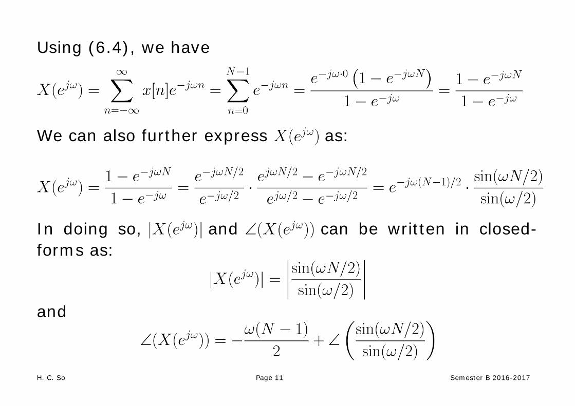
Using (6.4), we have
We can also further express as:
In doing so, and can be written in closed-forms as:
and

H. C. So Page 12 Semester B 2016-2017
Although is real, its phase is if it is negative while the phase is 0 if it is positive.
Note that we generally employ (6.8) and (6.9) for magnitude and phase computation.
In using MATLAB to plot and , we utilize the command sinc so that there is no need to separately handle the “0/0” cases due to the sine functions. Recall:
As a result, we have:

H. C. So Page 13 Semester B 2016-2017
The key MATLAB code for is N=10; %N=10 w=0:0.01*pi:2*pi; %successive frequency point
%separation is 0.01pi dtft=N.*sinc(w.*N./2./pi)./(sinc(w./2./pi)).*exp(-j.*w.*(N-1)./2); %define DTFT function subplot(2,1,1) Mag=abs(dtft); %compute magnitude plot(w./pi,Mag); %plot magnitude subplot(2,1,2) Pha=angle(dtft); %compute phase plot(w./pi,Pha); %plot phase There are 201 uniformly-spaced points for plotting the continuous functions and .

H. C. So Page 14 Semester B 2016-2017
0 0.2 0.4 0.6 0.8 1 1.2 1.4 1.6 1.8 20
5
10
15
ω (π)
|X|
Magnitude spectrum
0 0.2 0.4 0.6 0.8 1 1.2 1.4 1.6 1.8 2-4
-2
0
2
4
ω (π)
∠ X
Phase spectrum

H. C. So Page 15 Semester B 2016-2017
Example 6.4 Find the inverse DTFT of which is a rectangular pulse. Within the period of , has the form of:
where .
Using (6.6), we get:
That is, is an infinite-duration sequence whose values are drawn from a scaled sinc function.
Note also that corresponds to the discrete-time version in Example 5.2.

H. C. So Page 16 Semester B 2016-2017
Example 6.5 Given a discrete-time finite-duration sinusoid:
Find the tone frequency using DTFT. Consider the continuous-time case first. According to (5.10), the Fourier transform pair for a complex continuous-time tone of frequency is:
That is, can be found by locating the peak of the Fourier transform. Moreover, a real-valued tone is:

H. C. So Page 17 Semester B 2016-2017
This means that and can be found from the two impulses of the Fourier transform of .
Analogously, we expect that there are two peaks which correspond to frequencies and in the DTFT for .
The MATLAB code is N=21; %number of samples is 21 A=2; %tone amplitude is 2 w=0.5*pi; %frequency is 0.5*pi p=1; %phase is 1 n=0:N-1; %define a vector of size N x=A*cos(w*n+p); %generate tone for k=1:2001 %frequency index k w=(k-1)*pi/1000; %frequency interval of [0,2pi]; %compute DTFT at frequency points w only e=(exp(j.*w.*n)).'; %construct exponential vector X(k) = x*e; end

H. C. So Page 18 Semester B 2016-2017
X=abs(X); %compute magnitude k=1:2001; f=(k-1)./1000; plot(f,X) Note that is continuous in and we cannot compute all points. Instead, here we only compute at
for . That is, k corresponds to frequency w=(k-1)*pi/1000. With the use of max(abs(X)), we find that the peak magnitude corresponds to the index k=501, then the signal frequency is correctly determined as:

H. C. So Page 19 Semester B 2016-2017
0 0.2 0.4 0.6 0.8 1 1.2 1.4 1.6 1.8 2
0
2
4
6
8
10
12
14
16
18
20
radian frequency (π)
|X|

H. C. So Page 20 Semester B 2016-2017
Properties of DTFT
Linearity
If and are two DTFT pairs, then:
(6.10) Time Shifting
A shift of in causes a multiplication of in :
(6.11) Time Reversal
The DTFT pair for is given as:
(6.12)
H. C. So Page 21 Semester B 2016-2017
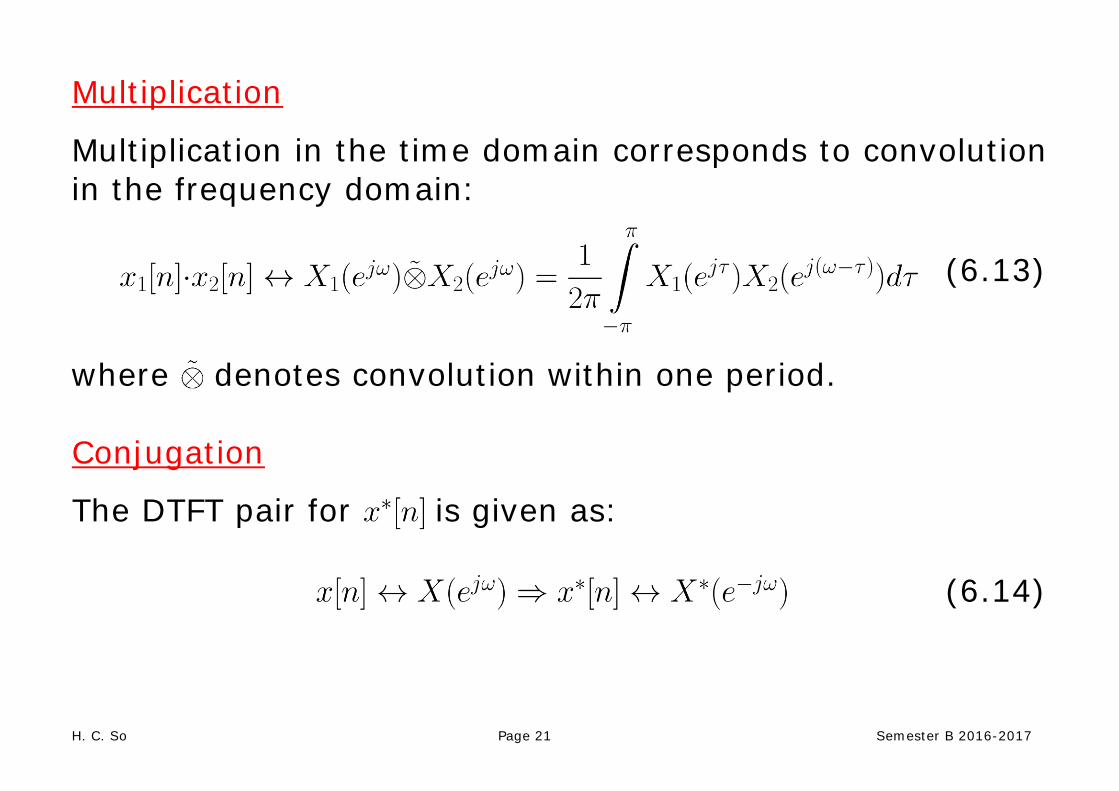
Multiplication
Multiplication in the time domain corresponds to convolution in the frequency domain:
(6.13)
where denotes convolution within one period. Conjugation
The DTFT pair for is given as:
(6.14)

H. C. So Page 22 Semester B 2016-2017
Multiplication by an Exponential Sequence
Multiplying by in time domain corresponds to a shift of in the frequency domain:
(6.15)
Differentiation
Differentiating with respect to corresponds to multiplying by :
(6.16)
Parseval’s Relation
The Parseval’s relation addresses the energy of :
(6.17)

H. C. So Page 23 Semester B 2016-2017
With the use of (6.6), (6.17) is proved as:
(6.18)

H. C. So Page 24 Semester B 2016-2017
Convolution
If and are two DTFT pairs, then:
(6.19) which can be derived as:
(6.20)
H. C. So Page 25 Semester B 2016-2017
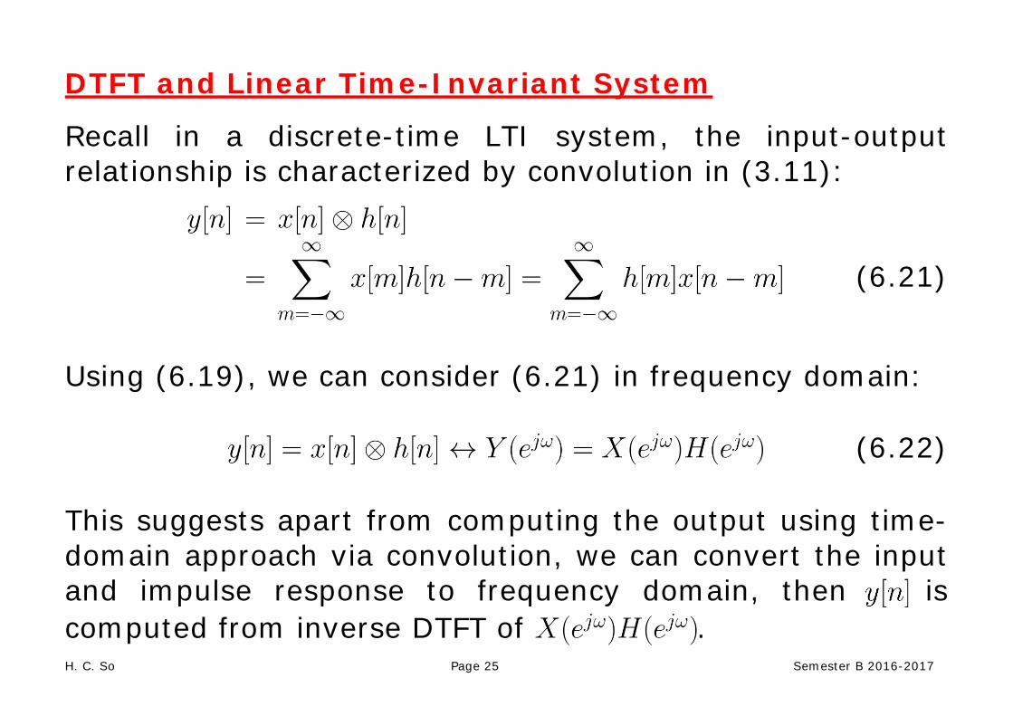
DTFT and Linear Time-Invariant System
Recall in a discrete-time LTI system, the input-output relationship is characterized by convolution in (3.11):
(6.21)
Using (6.19), we can consider (6.21) in frequency domain:
(6.22)
This suggests apart from computing the output using time-domain approach via convolution, we can convert the input and impulse response to frequency domain, then is computed from inverse DTFT of .

H. C. So Page 26 Semester B 2016-2017
In fact, represents the LTI system in the frequency domain, is called the system frequency response. Recall (3.22) that the input and output of a discrete-time LTI system satisfy the difference equation:
(6.23)
Taking the DTFT and using the linearity and time shifting properties, we get:
(6.24)

H. C. So Page 27 Semester B 2016-2017
The system frequency response can also be computed as:
(6.25)
Example 6.6 Determine the system frequency response for a causal LTI system described by the following difference equation:
Applying (6.25), we easily obtain:

H. C. So Page 28 Semester B 2016-2017
Example 6.7 The moving average (MA) is in fact a LTI system. Consider the close price of Dow Jones Industrial Average (DJIA) index as input and the output is the 20-day MA. Establish the input-output relationship using a difference equation. Then compute the system impulse response and frequency response. Plot the system magnitude frequency response. In stock market (or other applications), future data are unavailable. The best we can do is to use the today value and close prices of previous 19 trading days in MA calculation, that is:

H. C. So Page 29 Semester B 2016-2017
Following Example 3.18, we can easily deduce the impulse response as:
Applying (6.25), the system frequency response is:
From the magnitude plot, the frequency is concentrated around the DC. It is called a lowpass filter (also for Example 6.3).
From Fig. 1.11, we see that low-frequency components (smooth part) are kept while high-frequency components (fluctuations) are suppressed in the system output.
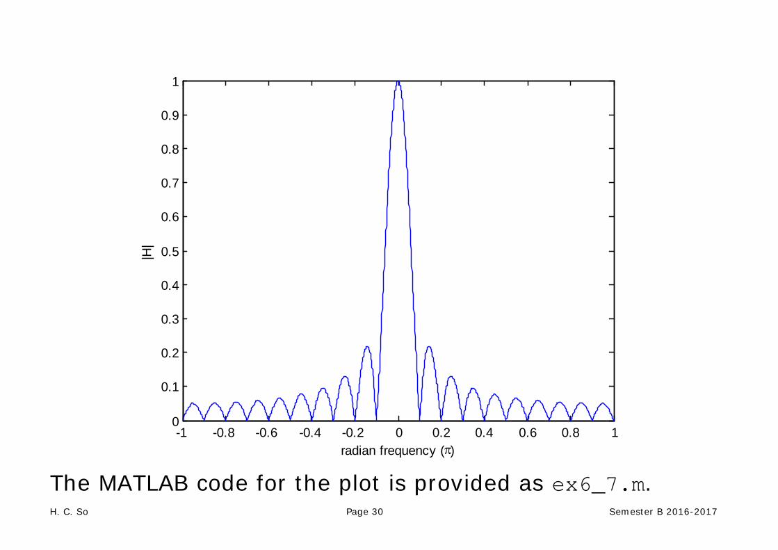
H. C. So Page 30 Semester B 2016-2017
The MATLAB code for the plot is provided as ex6_7.m.
-1 -0.8 -0.6 -0.4 -0.2 0 0.2 0.4 0.6 0.8 10
0.1
0.2
0.3
0.4
0.5
0.6
0.7
0.8
0.9
1
radian frequency (π)
|H|