Discrete Public Goods under Threshold Uncertainty:

Theory and Experiment

Michael McBride1

University of California, Irvine

Current version: November 2004

Abstract: A discrete public good is provided when total contributions exceed

the contribution threshold. I show that for a large class of threshold probability

distributions, an increase in threshold uncertainty by 2nd-order stochastic dom-

inance will increase (decrease) equilibrium contributions when the public good

value is su ciently high (low). In an experiment designed to test these predic-

tions, behavior only moderately verifies the predictions. Using elicited beliefs

data to represent subjects’ beliefs, I find that behavior is not consistent with

expected payo maximization, however, contributions are increasing in subjects’

subjective pivotalness. Thus, wider threshold uncertainty will sometimes–but

not always–hinder collective action.

JEL Classifications: C72, C90, D80.

Keywords: collective action, participation, experiments, elicited beliefs.

1Department of Economics, University of California, Irvine, 3151 Social Science Plaza, Irvine, CA, 92697-5100, mcbride@uci.edu. Helpful comments were received from Stephen Morris, Ben Polak, David Pearce,Hongbin Cai, Andrew Schotter, Thomas Palfrey, Charles Plott, Dirk Bergemann, Leatt Yariv, Chris Udry,Pushkar Maitra, seminar participants at Yale University’s game theory group, UCSB third-year seminar,BYU, UC Irvine, Ohio State, Stanford Graduate School of Business, participants at the 2004 Public ChoiceSociety / Economic Science Association Meetings, and two anonymous referees. Financial support wasreceived from the Institution for Social and Policy Studies at Yale University, the California Social ScienceExperimental Laboratory (CASSEL) at UCLA, and the University of California, Irvine. Special thanks tothe Social Science Experimental Laboratory at the California Institute of Technology and CASSEL for useof laboratory resources and to Yolanda Huang for programming assistance.

1

1 Introduction

The ability or inability of groups to act collectively explains a variety of social phenomena,

from cartels to military coups, from economic policies to social norms, and from political

institutions to social activism. As such, researchers seeking to explain these and other

phenomena have looked for preconditions for successful collective action. Since Olson’s

(1965) seminal work, economists have examined how a number of factors, such as group

size, excludability, selective incentives, punishment, and so on, inhibit or foster collective.2

One factor that potentially a ects individuals’ decisions to participate in a collective action

is uncertainty about the threshold level of contributions needed for successful action. For

example, neighborhood residents will not know how many individual requests to City Hall

will be required to install a tra c signal at a local intersection; citizens might not know

the amount of money required to complete a public project; or, more dramatically, coup

plotters will not know how big their faction needs to be to overthrow the incumbent dictator.

Previous research has acknowledged that threshold (or provision) uncertainty can a ect

collective action. Nitzan and Romano (1990) conduct the first theoretical study of the topic.

They model the setting as a discrete (step-level) public good game in which the threshold

is chosen randomly from a commonly known threshold distribution and where voluntary3

contributions are made simultaneously. They find that initial increases in threshold un-

certainty (e.g., a wider variance in the threshold distribution) will often, but not always,

be matched by increased contributions, and that e cient equilibria often still. A second

theoretical study by Suleiman (1997) finds a similar result for the simplified game with a uni-

2There are many strands of collective action research. See Sandler (1992) for general presentation ofcollective action from the economics perspective. Another formal approach di erent from the discrete publicgood analysis used here that is often by sociologists to explain riots and revolutions is the threshold or tippingmodel, as in Granovetter (1978), Yin (1998), and Chwe (1999, 2000). A di erent methodological approachto study collective action is one that focuses on authority and structure (Lichbach 1998).

3The focus on voluntary participation can be justified. By leaving aside other possible factors (e.g.,punishment), this focus allows for identifying the fundamental e ect of threshold uncertainty on individuals’incentives to participate in an institution-free environment. This serves as a useful benchmark and canprovide direction for future researchers to identify how groups can or should act to overcome or complementthese e ects. Moreover, there is already an established body of research that focuses on voluntary partic-ipation collective action as discrete public good games, so my findings can compare directly with existingfindings.

2

form threshold distribution. There have also been experimental studies. Wit and Wilke’s

(1998) and Au’s (2004) conducted experiments with sequential contributions, and they find

that contribution levels are lower under higher threshold uncertainty. Gustafsson, Biel,

and Garling (1998) report a similar finding in an analogous experiment with simultaneous

contributions. Finally, Suleiman, Budescu, and Rapoport (2001) find in a simultaneous

contributions experiment that the e ect of threshold uncertainty can depend on the mean

of the threshold distribution. When the mean is low, increasing uncertainty can increase

contributions, but the reverse holds when the mean is high.

This paper presents a theoretical and experimental study of an unexplored aspect of this

issue–how the e ect of increased threshold uncertainty on contributions depends on the

value of the public good. My theoretical analysis yields a preliminary prediction: a small

increase in threshold uncertainty will actually increase voluntary participation when indi-

viduals’ benefits of successful action are su ciently large, but it will decrease participation

when the benefits are small. Like Nitzan and Romano (1990), I obtain my findings by

building on Palfrey and Rosenthal (1984), who first modeled collective action as voluntary

contributions towards a discrete public good. They show that with a commonly known

threshold there always exists an e cient (Nash) equilibrium, although ine cient equilibria

can also exist. I add threshold uncertainty to their model and examine how (Bayesian Nash)

equilibrium contributions change as the threshold uncertainty changes. In particular, when

the value of the public good is su ciently large, an increase in threshold uncertainty (i.e., by

second order stochastic dominance) increases an individual’s probability of being a pivotal

contributor, thereby increasing the probability she will contribute and driving up equilib-

rium contributions. When the value of the public good is small, the uncertainty increase

will decrease the probability of being pivotal.

I test these predictions using data collected from a laboratory experiment. My experi-

ment, although not the first to vary threshold uncertainty (see references above), is the first

to vary both threshold uncertainty and the value of the public good. Thus, it provides me

with the best available data to test the above predictions. Overall, the data moderately

verify those predictions: contribution levels under one threshold probability distribution

3

usually di er from contributions under another distribution as qualitatively predicted by the

theoretical model. However, the predictions are not always verified. Two questions follow:

why are the predictions verified to any degree, and why is that level of verification so weak?

I address these questions using data on subjects’ elicited beliefs about other players’ contri-

bution levels. An examination of these data reveals that subjects do update their reported

beliefs in manners consistent with many learning models. This finding justifies using these

data to proxy for subjects’ true beliefs, which in turn allows me to calculate subjects’ implied

subjective probabilities of being pivotal. Conditioning on this subjective pivotalness, I show

that subjects do not behave in a manner consistent with the model’s implied decision rule.

While this fact weakens the predictive power of the model, an important qualitative feature

of the model is observed: contributions are increasing in subjects’ subjective pivotalness.

Thus, when making contribution decisions, individuals do think strategically in that they

care about pivotalness.

The overall conclusion is that threshold uncertainty does not necessarily inhibit collective

action for two reasons: first, individuals are successful, to some degree, in relating changes in

threshold uncertainty into changes in subjective beliefs about pivotalness, and second, indi-

viduals do respond to pivotalness, even if not to the degree implied by the model. However,

threshold uncertainty in some settings–particularly when the public good is low-valued–is

likely to hinder collective action. This has both positive and negative implications con-

cerning actual groups’ abilities to act collectively. Successful collective action may occur in

the face of threshold uncertainty even when participation is voluntary and uncoordinated,

however, when the value of the public good is low, a potentially costly reduction in threshold

uncertainty may be necessary for successful action unless there are other mitigating factors

(e.g., selective incentives, punishment, etc.).

This paper fits best in the literature that considers the role of uncertainty in collective

action. Previous work has examined, among other things, uncertainty about other individu-

als’ altruism (Palfrey and Rosenthal 1988), uncertainty about other individuals’ contribution

costs (Palfrey and Rosenthal 1991), and uncertainty about other individuals’ valuations of

4

the public good (Menezes, Monteiro, and Temimi 2001).4 My theoretical work is closest

to Nitzan and Romano (1990), the di erence being that I have each player make a binary

contribution choice, which better represents collective action scenarios that involve partici-

pation, in-out, or yes-no decisions instead of continuous contributions, which better represent

monetary contributions. I show how this di erence has e ciency implications. Finally,

my work is also closely related to the theoretical and experimental work on common pool

resources (CPRs) with unknown pool size (e.g., see Budescu, Rapoport, and Suleiman 1995).

2 Model

The discrete public good game consists of the following. The set of expected payo max-

imizing players is N = {1, ..., n}, 2 < n < . Players have identical binary action sets

Ai = {0, 1}, with actions labeled {don’t contribute, contribute} . When players mix overthose actions, let i be the probability that ai = 1 (i contributes). The cost of contributing

c and the value of a provided public good v are the same for all individuals. The contribu-

tion threshold t to provide the public good is chosen from a publicly known distribution cdf

F with pdf f s.t. F (0) = 0. Given C realized contributions, the payo s are:

payo for i =

v if C t and ai = 0v c if C t and ai = 10 if C < t and ai = 0c if C < t and ai = 1

.

For most of this paper I use discrete threshold distributions, but assuming an underlying

continuous contribution will be necessary to consider what happens when the binary action

set assumption is relaxed in Section 3.4.5

The timing of the game is as follows: (1) n, v, c, F , and the game set-up are commonly

known; (2) the players simultaneously choose whether or not to contribute; (3) payo s are

received. The analysis focuses on Bayesian Nash equilibria.

4Palfrey and Rosenthal (1988, 1991) examine discrete contributions. Menezes, Monteiro, and Temimi(2001) build on Bagnoli and Lipman (1989) in considering continuous contributions.

5The analysis is unchanged if the discrete F is actually a discrete representation of an underlying con-tinuous threshold distribution. For example, consider a continuous cdf H (x) with pdf h (x) over (0, ).Then F the discrete version of H (with pdf h (x)) is calculated s.t. F (x) =

R x0h(x)dx for all x = {1, 2, ...} .

5

3 Analysis

The number of contributions in equilibrium is of greater interest than which players con-

tribute in equilibrium. I will treat two equilibria with the same number of contributions as

a unique equilibrium.

Sections 3.1-3 assume that the threshold distribution is strictly quasi-concave. Formally,

denote cdf F strictly quasi-concave if its pdf is single-peaked and if f (x) 6= f (x+ 1) for

any f (x) > 0, while the pdf can be flat at any x where f (x) = 0.6 The main results in

this paper can be obtained without this condition (see Section 3.4), but this condition is not

unrealistic and greatly simplifies the analysis.

3.1 Pure Equilibria

For now, the focus is on pure equilibria. An agent’s decision in equilibrium will depend on

the probability she is pivotal in providing the public good. Denote C i to be the set of

contributing agents besides i. The payo matrix is

C i < t 1(lost cause)

C i = t 1(pivotal)

C i > t 1(redundant)

spend c v c v ckeep 0 0 v

.

Let a i = (a1, ..., ai 1, ai+1, ..., an). Further denote Pr[piv|a i, F ] the probability that i

is pivotal given a i and F , Pr[lost|a i, F ] the probability of a lost cause, and Pr[red|a i, F ]

the probability of being redundant:

Pr [piv|a i, F ] =Xx=1

(Pr [C i = x 1|a i] f (x))

Pr [lost|a i, F ] =Xx=1

(Pr [C i < x 1|a i] f (x))

Pr [red|a i, F ] =Xx=1

(Pr [C i > x 1|a i] f (x)) .

6To illustrate, a uniform pdf over {3, 4} is single-peaked, but it is not strictly quasi-concave because it isflat at f (3) and f (4).

6

Given a i and F , a player is willing to contribute if her expected payo contributing exceeds

that of not contributing:

Pr [lost|a i, F ] ( c) + Pr [piv|a i, F ] (v c) + Pr [red|a i, F ] (v c) Pr [red|a i, F ] v

Pr [piv|a i, F ]c

v.

It follows that for each i in a pure Nash equilibrium:

ai =0 if Pr [piv|a i, F ] <

cv

a0 {0, 1} if Pr [piv|a i, F ] =cv

1 if Pr [piv|a i, F ] >cv

(1)

Denote a pure equilibrium by C , and (abusing notation) let C also signify the number

of contributions in that equilibrium. In a pure equilibrium C a contributing player believes

with probability one that exactly C 1 others are contributing. Thus, that player is pivotal

with probability f (C ). A non-contributing player is pivotal with probability f (C + 1).

It follows that conditions for existence of an equilibrium C are:

C =0 if f (1) c

v

x {1, .., n 1} if f (x) cvand f (x+ 1) c

v

n if f (n) cv

. (2)

Proposition 1 contains some preliminary conditions for uniqueness of equilibria. In it

and throughout the rest of the paper, the feasible mode m is the mode of the distribution

over x {1, ..., N}. More formally, x N is the feasible mode where f (x) > f (x0) for all

x0 N , x0 6= x (“>” by strict quasi-concavity).

Proposition 1: (Uniqueness of Pure Equilibria) Fix N , c, v, and F .

(a) The unique equilibrium is C = 0 i cv> f (m). The unique equilibrium is

C = n i cv< f (x) for all x N .

(b) If F is strictly quasi-concave, then any non-zero equilibrium has C m.

(c) If F is strictly quasi-concave, then there is at most one non-zero equilibrium

with C > 0. Furthermore, if there is more than one equilibrium then there are

exactly two equilibria: the trivial equilibrium C = 0 and a non-zero equilibrium

C > 0.

7

Proof: (a) Follows directly from the conditions in (2).

(b) By (2), any interior equilibrium C > 0 must have f (C ) cv

f (C + 1).

By strict quasi-concavity, C must thus be to the right of m where the pdf is

“downward sloping.”

(c) Suppose two non-zero equilibria C and C 0 s.t. C 0 > C > 0. From (2), it

must be true that (i) f (C ) cv, (ii) f (C + 1) c

v, and (iii) f (C 0) c

v. But

(i)-(iii) cannot be all be true since f is strictly quasi-concave. A contradiction.

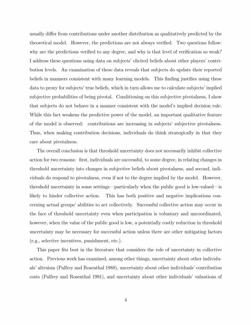
Figure 1(a) illustrates the equilibria. In this figure, there is a trivial equilibrium C = 0

since f (1) < cv. That is, if no one else contributes, then a single contribution is very unlikely

to lead to provision, so no individual will contribute. The non-trivial equilibrium is C = 3.

Each of the three contributors is willing to make her contribution given that two others are

contributing since her probability of being pivotal is higher than cv. Any non-contributor

is not willing to contribute given that three others contribute since her probability of being

pivotal is less than cv. Also, notice that for a strictly quasi-concave distribution, a non-zero

equilibrium must be to the right of the feasible mode m = 3 (on the downward-sloping

side of the pdf). This fact follows from the features of the equilibrium described in (2):¡f (C + 1) c

v

¢so that f (C ) c

v> f (C + 1).

Hereafter, we will focus on the non-trivial equilibrium C . From Proposition 1(c), a zero-

contribution equilibrium is non-trivial only if cvis higher than the feasible mode. Otherwise,

the non-trivial equilibrium has contributions. As shown later, this non-trivial equilibrium

is the Pareto-undominated equilibrium, although it can be ine cient.

I now state the two main theoretical propositions of this paper. The first of these will

consider a threshold distribution that is totally feasible. Say that F is totally feasible when

the public good can be provided with probability 1, i.e., F (n) = 1.

Proposition 2: (2nd-order Stochastic Dominance) Fix N, c, and v, and con-

sider two strictly quasi-concave threshold distributions F and bF , F 6= bF . DenoteC and bC the respective non-trivial equilibria. If (i) F 2nd-order stochastically

dominates bF , (ii) F and bF have the same mean, and (iii) F and bF are both

8

totally feasible, then there exists a scalar k > 0 such that bC C if the cost-

value ratio cv

k. Furthermore, if it is also true that the feasible mode of F

is strictly greater than the feasible mode of bF , then there exists a second scalark0 k such that C bC if the cost-value ratio c

v> k0.

Proposition 3: (Single-Crossing Condition) Fix N, c, and v, and consider

two strictly quasi-concave threshold distributions F and bF , F 6= bF, with feasiblemodes m and bm, respectively. Denote C and bC the respective non-trivial

equilibria. If f (m) > bf (bm) and f and bf cross exactly once over {m, ..., n},then there exists a scalar k > 0 such that bC C if c

vk, and C bC if

cv> k.

The proofs of Proposition 2 and 3 will follow directly from a more general result, Lemma

1, about games that di er only in their threshold distributions. In the rest of Section 3.1, I

establish Lemma 1, after which Propositions 2 and 3 will be proven.

Because C m, we can restrict our attention to that part of the threshold pdf that is

betweenm and n. And we can go one step further when comparing the non-trivial equilibria

of otherwise identical games with di erent threshold distributions. The following corollary

to Proposition 1 states that when looking for the equilibrium with higher contributions of

the two games, we can restrict our attention to that part of the two distributions that is

between the feasible mode with higher mass and n. In other words, if f (m) > bf (bm), thenwe need only be concerned with the range {m, ..., n}. Denote em the feasible mode with

higher mass.

Corollary 1: (Comparing Non-trivial Equilibria) Fix N, c, and v, and consider

two strictly quasi-concave threshold distributions F and bF , F 6= bF . Denote Cand bC the respective non-trivial equilibria.

(a) bC > C i there exists some level of contributions x {C + 1, ..., n}, suchthat bf (x) c

v.

(b) If bC > C then bC em.9

With our attention now restricted to the right of the feasible mode with higher mass, we

look more closely at the behavior of the two distributions from em to n. I will refer to this

specific area as the interior I = {em, ..., n}. One key condition of interest is when one of

the pdf’s has a higher interior-right tail, that is, one pdf is greater than the other pdf for all

contribution levels from some number in the interior I to n. The “interior-right” means that

we are looking at the right tail in this interior I. Another key condition is as analog for the

interior-left, but this condition will also be defined by the height of the pdf’s to the right of

the interior-left. After formally defining these conditions, I will illustrate them graphically.

Interior Tails Conditions: Consider two strictly quasi-concave distributions

F and bF , F 6= bF , and the resulting interior I = {em, ..., n}.(a) Say that bf has a fatter interior-right tail than f if there exists an x I,

such that bf (x0) f (x0) for all x0 {x, ..., n}.

(b) Say that f has a fatter interior-left tail than bf if there exists an x I,

such that (i) f (x0) bf (x0) for all x0 {em, ...x}, and (ii) if bm > m withbf (bm) > f (bm), then m f (x0) > bf (bm) for all x0 {em, ..., x}.Figure 2(a) illustrates these conditions with smooth pdf’s drawn for clarity. It shows the

case where both a fatter interior-right tail IR and a fatter interior-left tail IL exist. Notice

that these tails do not necessarily meet. Figure 2(b) shows that we cannot distinguish IR

from IL when one pdf is always above the other in I. Figures 2(c)-(d) show that the tails

meet when the pdfs cross once in the interior. The reason for condition (ii) in a fatter

interior-left tail is that we want to know when the non-trivial equilibrium C will be in that

interior-left tail and when C bC . This idea is illustrated on Figure 2(b). Notice that if

cv= k1, then bC is higher than C = x1 even though f (x1) > bf (x1). This is because x1 is

to the left of the feasible mode of bF .We can use these figures to demonstrate the two main propositions of the paper and

bring us closer to Lemma 1. Notice that the k and k0 in Figure 2(a) satisfy the k and k0 in

Proposition 2. F 2nd-order stochastically dominates bF , and F has a higher feasible mode.We see that if c

vk then bC C , whereas if c

v> k0 then C bC .

10

Lemma 1: (Fatter Interior Tails and Pure Equilibria) Consider two games

that are identical except for their strictly quasi-concave threshold distributions F

and bF , F 6= bF . Denote C and bC the respective non-trivial equilibria.

(a) If bf has a fatter interior-right tail than f , then there exists a scalar k,0 < k < 1, such that bC C if the cost-value ratio c

vk.

(b) If f has a fatter interior-left tail than bf , then there exists a scalar k0,0 < k0 < 1, such that C bC if the cost-value ratio c

v> k0.

Proof: (a) Suppose the contrary, that bf has the fatter interior-right tail butC > bC for some c

vk. Choose k = f (bmR), where bmR is the mode of bf

over the fatter interior-right tail {x, ..., n}. It follows that cv

k implies that

C x, where x is the beginning of the fatter interior-right tail. For C > bC ,

it must be that f (x0) cv> bf (x0) for some x0, x x0 n, but this contradicts

the fact that bf has a fatter interior-right tail. Similar logic will show that any

kh0, bf (bmR)

iwill satisfy the claim.

(b) Follows from logic similar to that used in part (a).

Lemma 1(a) says that contributions will be higher under the distribution with the fatter

interior-right tail if cvis su ciently small, Lemma 1(b) says that contributions will be higher

under the distribution with fatter interior-left tail if cvis su ciently large. The reason is

that the fatter tail implies a higher probability of being pivotal at the contribution levels in

the tail. We can now prove Propositions 2 and 3.

Proof of Proposition 2: F 2nd-order stochastically dominates bF implies thatPx0x=0

bF (x) Px0x=0 F (x) for all x

0 N. Total feasibility and same means

together imply thatPn

x=0bF (x) = Pn

x=0 F (x) (see La ont 1989). Subtracting

the first condition from the second condition yields

nXx=0

bF (x) x0Xx=0

bF (x) nXx=0

F (x)x0Xx=0

F (x)

nXx=x0+1

bF (x) nXx=x0+1

F (x) .

11

This last equation says that, starting from n and moving to the left on the graph

of the cdf’s, when F and bF first separate, bF must be below F . This implies thatbf must have a fatter interior-right tail than f . (Notice that if F and bF do notseparate in interior I, then bf and f have identical interiors, which means that bfhas a fatter interior-right tail by the weakness.) Since bf has a fatter interior-right tail, invoking Lemma 1 establishes that there exists a k that satisfies the

first claim in Proposition 2.

If the feasible mode of f has mass strictly greater than the feasible mode

of bf then it follows that f has a fatter interior-left tail. Invoke Lemma 1 to

establish that there exists a k0 as in the second claim in Proposition 2.

The intuition for Proposition 2 is straightforward. Spreading the distribution pushes

probability mass to the right part of the tail, and the total feasibility restriction means that

this mass will stay in the feasible region. With more mass in the interior-right tail, the

probability of being pivotal is higher at the high levels of x. Alone, this is not enough to

ensure that contributions will be higher in the game with the spread probability. If the

cost-value ratio cvis too high, then the mass increase on the right will not be enough, and

there might be a drop in contributions. This is seen in Figure 2(a) when cv> k0. If the

cost is low enough (below k) then contributions are higher.

Notice that total feasibility is su cient but not necessary. What is necessary in this case

of a mean-preserving spread is that enough mass is spread to the interior-right. In other

words, all we need for Proposition 2 is a fatter interior-right tail (Lemma 1). Proposition 3

demonstrates this point (because it does not assume total feasibility) while making another

claim about an implication of the single-crossing property.

Proof of Proposition 3: The claim assumes that I = {m, ..., n} (i.e., em = m).Suppose the pdf’s cross at x {m, ..., n}, so that f (x0) bf (x0) for all m x0 <

x, and f (x00) f (x00) for all x x00 n. It follows then that bf has a fatterinterior-right tail and f has a fatter interior-left tail. It remains to show that

k = k0 in Lemma 1.

12

If f (bm) bf (bm) then by strict quasi-concavity, f has a fatter interior-lefttail from m to x + 1 and bf has a fatter interior-right tail from x to n. These

two tails meet each other, so k = k0 in Lemma 1, thus satisfying the claim. Now

suppose that f (bm) < bf (bm) (akin to Figure 3.2(b)). Set k = bf (bm), and thenfind where f crosses k. For any c

vk, we satisfy Lemma 1(a), and for any

cv> k, we satisfy Lemma 1(b). Thus k = k0 in Lemma 1.

Proposition 3 applies for a wide variety of threshold distributions. For example, many

monotone mean-preserving spreads will meet this single-crossing condition, such as shown

in Figure 2(d). Also, the class of uniform threshold distributions meets this single-crossing

condition. I take advantage of this last fact in the experiment I conducted (see Section 4).

3.2 Mixed Equilibria

Similar logic is used in examining the mixed equilibria, but there is one important di erence.

While the results for pure equilibria come from looking at fatter interior tails of the proba-

bility distributions, the results for the mixed equilibria come from looking at fatter interior

tails of transformations of the probability distributions.

For reasons given below, when looking at mixed equilibria, we can restrict our attention

to symmetric equilibria. With i the probability that player i contributes, we now let

= i = j, for all i, j N , be the rate at which every player mixes. From (1), we see

that the conditions for a symmetric equilibrium are

i =0 if Pr [piv| = 0, F ] < c

v0 [0, 1] if Pr [piv| = 0, F ] = cv

1 if Pr [piv| = 1, F ] > cv

. (3)

The transformation of the probability distribution of interest is what I will call the

Pr[piv|F ]-curve. This curve maps the probability player i is pivotal given that all others aremixing at rate [0, 1] . Figure 1(b) illustrates this Pr[piv|F ]-curve for the pdf in Figure1(a). This curve is derived as follows:

Pr [piv| , F ] =nXx=1

µn 1

x 1

¶x 1 (1 )n x f (x) .

13

With N = 5, there are three symmetric equilibria in Figure 1(b): = 0, = 0.32, and

= 0.91. From the conditions in (3), it follows that symmetric equilibria can only occur

at three places on the graph: at the origin if the Pr[piv|F ]-curve is less than cvat = 0, at

a place where the Pr[piv|F ]-curve intersects the cv-line, and at = 1 if the Pr[piv|F ]-curve

crosses it above cv. This last possibility would happen in Figure 1(b) if c

v0.15.

Equilibria at 0 and 1 have a nice stability property: an increase in from 0 would drive

contributions back down to zero, and an decrease in from 1 would drive contributions

back to one. Strictly mixing equilibria only share this property if the slope of the Pr[piv|F ]-curve is downward sloping where it crosses the c

v-line. In Figure 1(b), the equilibrium at

0.32 is not stable, but the one at 0.91 is stable. The stable symmetric equilibria have

qualitative properties similar to the pure equilibria: they occur where the distribution (or

its Pr[piv|F ]-curve transformation) crosses the cvline from above. We take advantage of

this fact in the propositions and corollaries for symmetric equilibria.

This stability notion coincides with the concept of evolutionarily stable strategies (ESS)

(see Gintis (2000)): i is at least as better o playing than playing the perturbed strategy

given that the others play , and if i is indi erent to playing the perturbed strategy given the

other play , then i is strictly better o playing than playing the perturbed strategy when

all others play the perturbed strategy. I now use this stability concept to state Proposition

1A, which is the Pr[piv|F ]-curve analog to Proposition 1, with the addition of part (0).

Proposition 1A: (Uniqueness of Symmetric Equilibria) Fix N , c, v, and F .

(0) If there is a stable equilibrium in which at least two players i and j are

strictly mixing i , j (0, 1), then it must be that i = j (generically).

(a) The unique equilibrium is = 0 i cvis strictly greater than the maximum

of the Pr [piv|F ]-curve. The unique equilibrium is = 1 i cvis strictly less

than Pr [piv|F ]-curve for all [0, 1].

(b) If the Pr [piv|F ]-curve is strictly quasi-concave, then any stable equilibriumwith > 0 has (weakly) to the right of the mode of the Pr [piv|F ]-curve.

14

(c) If the Pr [piv|F ]-curve is strictly quasi-concave, then there is at most onestable equilibrium with > 0. Furthermore, if there is more than one stable

equilibrium then there are exactly two stable equilibria: the trivial equilibrium

= 0 and a non-trivial equilibrium > 0.

Proof: (0) Suppose an equilibrium with i and j both strictly mixing and

i < j . Equilibrium implies that each must have a probability of being pivotal

equal to cvby (3). Since j is mixing at a higher rate than i, i’s expected number

of contributors other than himself must be higher than j’s expected number of

contributors other than himself. However, this means that i and j do not have

equal probabilities of being pivotal (generically), which means that both cannot

have probabilities of being pivotal equal to cvwhich is a contradiction.

(a)-(c) Follows from logic used in proving Proposition 1.

I focus now on non-trivial equilibria that are stable and symmetric, and part (0) provides

justification. Any strict mixers must mix at the same rate, so if a mixed equilibrium is

asymmetric, the asymmetry is in who mixes and not the rate at which they mix. In fact,

the mixing rate in one of these asymmetric equilibria is the mixing rate in a symmetric

equilibrium of a transformed game.7 As a result, we are examining the main strategic

aspects8 of all mixed equilibria when considering symmetric equilibria. We can justify

looking at stable equilibria, too. First, the ESS concept has nice stability properties that

suggest that such strategies are more likely to be observed. Second, ESS can arise out of

many dynamic processes which again suggests they are more likely to be observed.9 Third,

7More precisely, if Nmix is the set of mixers and N1 is the set of pure contributors, then the rate at whichthe mixers is mixing is equal to the mixing rate in game G0 with f 0 (x) = f (x+ |N1|) for all x > 0.

8The only aspect missing is the possibility of a di erent number of strict mixers.9Here are two examples of dynamic processes that lead to an ESS being reached. The first example is

a restricted best-response dynamic process. Suppose in period t, each player chooses a best response tothe strategies of the previous period with the restriction that BRi,t [ai,t 1 , ai,t 1 + ] [0, 1] . Inother words, each player is restricted to making only small deviations from his previous period’s strategy.Without this restriction, players would jump back and forth between contributing and not contributing, andno mixed equilibrium would be reached. In these dynamics, only ESS will be reached if the system starts outof equilibrium. The second example of a dynamic process is based on the interpretation of mixed strategiesin terms of large population, random interaction models in which players only play pure strategies. Considera large population of players that is randomly divided into n-sized groups over a long period of time. If

15

symmetric mixed ESS will exhibit comparative static properties that are qualitatively similar

to the asymmetric pure equilibria thereby giving added justification to the comparative static

predictions of these equilibria.

The analog to the non-trivial pure equilibrium C is the non-trivial stable and symmetric

equilibrium . Lemma 1 can be restated as Lemma 1A in terms of the fatter interior tails

of the Pr[piv|F ]-curves.

Lemma 1A: (Fatter Interior Tails and Symmetric Equilibria) Consider two

games identical except for their threshold distributions F and bF , F 6= bF . Denoteand b the respective symmetric and stable non-trivial equilibria.

(a) If the Prhpiv| bFi-curve has a fatter interior-right tail than the Pr [piv|F ]-

curve, then there exists a scalar k, 0 < k < 1, such that b if the cost-value

ratio cv

k.

(b) If the Pr [piv|F ]-curve has a fatter interior-left tail than the Prhpiv| bFi-

curve, then there exists a scalar k0, 0 < k0 < 1, such that b if the cost-value

ratio cv> k0.

A 2nd-order stochastic dominance relationship between threshold distributions F andbF does not necessarily imply a 2nd-order stochastic dominance between the Pr[piv|F ]- andPrhpiv| bFi-curves. However, a dominance relationship between F and bF will generally imply

that the Prhpiv| bFi-curve has a fatter interior-right tail, and it is the fatter interior-right tail

that really matters. This means that there will generally exist the k that yields bwhenever c

vk, which is the symmetric equilibrium analog to Proposition 2.

Similarly, when m is strictly higher than bm, the mode of the Pr[piv|F ]-curve will oftenhave a higher mass than the mode of the Pr

hpiv| bFi-curve. This will result in a fatter

players that receive higher payo s reproduce at faster rates, convergence will occur to a population wherea fraction of the population that contributes towards the public good will be equal to the mixed strategyequilibrium. Each of these two examples have dynamics that will lead to convergence to identical equilibria,either mixed in the first model or pure but in the mixed proportions in the second model. Equilibria thatare not ESS cannot be sustained with pertubations under any evolutionary model. We therefore expect tosee actual behavior fall more in line with these ESS.

16

interior-left tail for the Pr[piv|F ]-curve, which is su cient for the existence of the k0 that

yields b whenever cv> k0, which completes the symmetric analog to Proposition 2.

3.3 E ciency

We are interested in the e ciency of equilibria when there is threshold uncertainty and

also in the comparative e ciency of equilibria under di erent threshold distributions. The

welfare criterion used here is the sum of expected utilities: W (C) = nF (C) v Cc.

Proposition 4: (E ciency) Fix N , c, v, and F . Assume F is strictly

quasi-concave.

(a) The non-trivial pure equilibrium C is Pareto-undominated in the class of

pure equilibria, and C is ine cient if C < n and cvn< f (C + 1) < c

v.

(b) The symmetric and stable non-trivial equilibrium is generically ine cient,

but it can yield higher expected welfare than the non-trivial pure equilibrium C .

Proof: (a) From Proposition 1(c), we know that if there is more than one pure

equilibrium, then one is C 0 = 0 while the other is, say, C > 0. The expected

welfare of C 0 = 0 is 0. Since it must be true that f (C ) cv, it must also be

true that F (C ) cv. This implies that the expected welfare of C is

nF (C ) v C c nc

vv C c = (n C ) c,

which is weakly greater than 0. Thus, C is Pareto undominated.

Consider the second claim in (a). Let C {1, ..., n 1} . By Proposition1, C is to the right of the feasible mode. By strict quasi-concavity, f (C )

cv> f (C + 1) f (C + k) for all 1 < k n C . This means that the largest

marginal welfare gain to be had by an increase in one contribution is from C to

C +1. Welfare is higher under C +1 when W (C + 1) > W (C ) . Doing the

algebra shows this to be equivalent to f (C + 1) > cvn. It follows that the C is

ine cient when cvn< f (C + 1) < c

v.

17

(b) That mixed equilibria are generically ine cient is trivial. That the sym-

metric equilibrium can yield higher expected welfare than the pure equilibrium

is illustrated by an example. Suppose n = 5, f (1) = 0.54, f (2) = 0.13,

f (3) = 0.12, f (4) = 0.11, f (5) = 0.10, and cv= 0.14. Then we can find that

C = 1, ' 0.5, W (C ) = 18.29, and W ( ) ' 23.

As is common in public good games, ine ciencies arise because the marginal gain to

an individual from contributing is di erent from the marginal social gain from that same

contribution. This di erence comes from the welfare function accounting for all players’

marginal gain’s instead of just one individual’s marginal gain. This ine ciency does not

arise when f (C + 1) < cv, C = n, or when F (C ) = 1. Notice that this implies that the

non-trivial equilibrium C is e cient when the threshold is known with certainty–a fact

already established by Palfrey and Rosenthal (1984). Their result is thus a special case of

the more general result in Proposition 4(a).

The symmetric equilibrium can have higher expected welfare when the pdf has a tail to

the right of C that is close to but under cv. This is the case in the example in part (b)’s

proof. The symmetric equilibrium has higher welfare because expected contributions are

higher, and the higher contributions leads to a higher probability of provision that more

than o sets the decline in welfare due to greater total contribution cost.

Because contributions can increase due to an increase in uncertainty, welfare can be

higher under an increase in uncertainty. Again, suppose that the initial distribution has a

right tail above C that is below cvbut above c

vnfrom C +1 to n or close to n. A widening

of uncertainty that drives up the right tail will increase contributions, and if the increase in

the probability of provision is su cient then there will be an increase in expected welfare.

3.4 Other Considerations

General Threshold Distributions. I have worked out the analogs to the main claims

for when the threshold distributions are not restricted by strict quasi-concavity. The added

complication is the non-uniqueness of non-trivial equilibrium. One way around this compli-

cation is to look at the equilibrium with the highest level of expected contributions. Doing

18

so allows us to do the same analysis as before on this high-contribution equilibrium. For

pure equilibria, this high-contribution equilibrium is the Pareto-undominated equilibrium,

and Lemma 1 and Propositions 2 and 3 can be restated exactly word for word substituting

only “high-contribution equilibrium” in place of “non-trivial equilibrium.” The analysis will

also be similar for symmetric equilibria.

Continuous Contributions. Nitzan and Romano (1990) allow individuals to make

continuous contributions. These continuous contributions can be likened to monetary con-

tributions, whereas binary contributions can be likened to participation decisions. Leaving

the binary case means we must consider the underlying threshold distribution. Proposition

5 assumes that the underlying threshold distribution is a continuous and strictly quasi-

concave threshold distribution function H from which the discrete transformations F and

F 0 are derived so as to assign mass over Ai and A0i, respectively.

Proposition 5: (Continuous Contributions, partly from Nitzan and Romano

(1990)) Consider two games identical except for their contribution sets Ai and

A0i. Assume that the threshold distribution function H is continuous. Suppose

binary contributions Ai = {0, 1} for all i in the first game, and assume continu-ous contributions A0i = [0, 1] for all i in the second game. Then expected welfare

is always (weakly) higher in the second game with continuous contributions.

I sketch the proof using Proposition 4 and a result from Nitzan and Romano (1990).

They show that in continuous contribution games we need to consider the maximum number

of possible contributions. I restrict players to contribute at most 1, thus making n the

maximum contributions. In their notation, H is continuous over [a, b], 0 < a < n. If

b n with continuous contribution game, then C = b, 10 the public good is provided with

probability 1, and the equilibrium is e cient. If b < n, then C = n and the public good

is provided with probability strictly less than 1. Proposition 4 says that things change

10Here C is the total contribution but not necessarily the number of contributors because C is notnecessarily an integer.

19

with binary contributions. First, with total feasibility (n b) then the equilibrium is only

e cient if f (b) cv. Second, if not totally feasible, then it is only e cient if f (n) c

v.

Essentially, the equilibrium under continuous contributions will always be e cient, but

the equilibrium is not always e cient under binary contributions. Consider a proposed

equilibrium C < b. In the binary case, a non-contributor considers if f (C + 1) is greater

than cv. Now in the continuous case, if the player considers a 1

2contribution, then he

compares f¡C + 1

2

¢with c

2vin his decision rule. More generally, it can be shown that for a

12mcontribution, the player’s decision rule will compare f

¡C + 1

2m

¢with c

2mv. As m ,

the c2mv-line converges to 0 and f

¡C + 1

2m

¢converges to f (C ). In the limit, the player he

will contribute an amount whenever f (C ) > 0. Thus, contributions will cover the whole

feasible domain of the threshold distribution. For symmetric equilibria, similar reasoning

will show that with continuous contributions, = bnwhen n b.

This logic implies that wider threshold uncertainty can only decrease e ciency for the

continuous contribution case (when b increases past n), while wider uncertainty can increase

e ciency under binary contributions (even if b goes past n). While this is a strikingly

di erent result, the underlying behavior and analysis in each case is the same. The di erence

lies in the fact that we do not always have complete provision of the public good in the binary

case due to the cv-line above the horizontal axis.

Risk Aversion. If players are risk averse then the free-rider e ect (the worry about

donating a redundant contribution) diminishes while the lost-cause e ect (the worry about

contributing to a lost-cause) amplifies. A qualitative result similar to Lemma 1 will hold, but

there is an important di erence. The decision rule (1) will not compare Pr [piv|a i, F ] with

cv. Instead of drawing a horizontal c

v-line, there will be a curve that varies by contribution

level. On the graph of the pdf, this curve will be decreasing over the domain of contribution

levels with f (x) > 0, and its slope and shape will depend on the size of the risk aversion.

Under extreme amounts of risk aversion, the slope becomes more negative and the whole

curve shifts up. With a change in uncertainty from F to bF , the curve will also change. Forthe analog to Lemma 1(a), our definition of the fatter interior-right tail will have to consider

20

not just the comparison pdf’s but also the comparison of these curves.

Sequential Contributions. Since there is no private information in this game, there

are not the normal informational issues involved in comparing simultaneous and sequential

equilibria. Sequential moves only allow players to condition on observed behavior. This

observation will matter when comparing a mixed equilibrium to a sequential equilibrium,

but any pure equilibrium of the simultaneous game is an equilibrium of any sequential move

game.11 The main results from Section 3.1 will thus still apply in the sequential move game.

Hence, the focus on simultaneous contributions in this paper is not missing other important

strategic issues (other than timing) that would arise in a sequential move game.

4 Experiment

Laboratory experiments provide the ideal setting to conduct a preliminary empirical test of

the model’s theoretical predictions–that contributions will be higher under wider thresh-

old uncertainty if the public good is of su ciently high value–since the experimenter can

control both the level of threshold uncertainty and also changes in that uncertainty. This

section presents the main findings from an experiment I conducted at the California Social

Science Experimental Laboratory. All subjects are drawn from the student population of

the University of California, Los Angeles.12

4.1 Experiment Design

Each experiment session consisted of 4 practice rounds and 30 real rounds,13 and each session

had either 25 or 30 students. All decisions were made over a computer network in a computer

currency called “tokens.” Subjects amassed tokens depending on the decisions and the

factors determined by the computer. At the end of the session, subjects were paid U.S.

dollars according to a pre-announced token/dollar exchange rate.

11Dekel and Piccione (2000) have a similar finding for voting games in symmetric binary elections.12The dialogue from the instructional period is available from the author upon request.13The exception is the 8/21 session which ended after 26 rounds.

21

In each round, the computer randomly and anonymously assigns the subjects into groups

of five, and each subject is given one computer token. Each subject’s computer then displays

the public good value and the threshold distribution. Subjects are told that the threshold

distribution is a range T =©t, ..., t

ªfrom which the computer will randomly and uniformly

select the true threshold. Subjects are told that the “threshold-met value” and “threshold

range” are the same for all individuals and groups in the room.

Before deciding whether to keep (do not contribute) or spend (contribute) the one given

token, each subject is asked to assign percentage probabilities to what the others in his or

her group will do.14 Since five subjects are in each group, a subject assigns probabilities

to the following five events: exactly 0 others in the group spend, exactly 1 other spends,

exactly 2 others spend, exactly 3 others spend, and exactly 4 others spend. Once the

assigned percentages add up to 100 percent and the subject confirms the entry, the subject

then makes the decision to keep or spend the one token. Tokens not spent in the current

round cannot be spent in later rounds. Subjects are not allowed to communicate with any

other subjects in the room during the practice or real rounds.

A subject’s payment for a given round has two parts. The first payment is based on the

accuracy of the reported beliefs, which is derived using a proper scoring rule. The exact

formula is

v

2

µbit (actualt)

1

2

¡bit (0)

2 + bit (1) + ...+ bit (4)2¢¶+ v

4,

where bit (e) , e = 0, ..., 4, is the percent assigned by i to the event that e others spend, and

bit (actualt) is the percent assigned to that x that actually occurs. The highest this payment

can be in a given round is v2, and the lowest is 0. The second payment in a given round is

that resulting from the contribution decisions. Letting C be the total realized contributions

in the group, this payment is:

v if C t and ai = 0v + 1 if C t and ai = 11 if C < t and ai = 00 if C < t and ai = 1.

14See Nyarko and Schotter (2000) for discussion of the validity of using elicited beliefs.

22

I consider five di erent value-threshold range (v, T ) combinations:

(3, {3}) , (3, {1, 2, 3, 4, 5})(6, {3}) , (6, {2, 3, 4}) , (6, {1, 2, 3, 4, 5}) ,

in a variety of di erent treatments. While v was held fixed in each session, T varied in

some sessions. Whenever the range was changed, it was fixed for the first 15 rounds, then

changed to another range, which was then held fixed for the rest of the session. Table

1(a) lists the expected payo maximization mixed equilibrium contribution levels under the

di erent (v, T )-combinations. It also lists the qualitative predictions: contributions should

be higher under (3, {3}) than (3, {1, 2, 3, 4, 5}) , and they should be successively higher under(6, {3}), (6, {2, 3, 4}), and (6, {1, 2, 3, 4, 5}). Table 1(b) lists the di erent treatments and

the number of sessions per treatment.

This design is the correct design to test my theoretical predictions for a number of reasons.

(1) This basic set-up, including n = 5 and uniform threshold range, matches that used in the

previous experimental studies of threshold uncertainty mentioned earlier. This establishes

continuity with the other studies. (2) The uniform threshold range is the best way to

model the threshold distribution since subjects understand a uniform distribution. The

uniform threshold range also implies single-crossing for both pure and symmetric equilibria,

and this single-crossing implies nice qualitative predictions of contribution movements with

changes in uncertainty (Proposition 3). (3) The chosen parameters profiles will allow for

high and low v and for high and low uncertainty. Data for all these scenarios are needed

to compare with the predictions. (4) Eliciting beliefs will allow for more direct testing of

the underlying behavior of the subjects. Providing incentives to report true beliefs adds

credibility to the beliefs data. (5) Group sizes are held constant to remove the e ects of

group sizes on contribution levels. (6) No information on others’ decisions or payments is

given and all decisions are made privately to remove social pressures or social comparisons

that might a ect behavior. (7) The maximum payment for beliefs is half as much as the

highest payment from the keep/spend decision. This should remove the motive for players

23

to play a game that maximizes the beliefs payment.15

4.2 Results

Findings 1-4 summarize the main results.

Finding 1: The predictions concerning contribution levels under di erent (v, T )-

combinations are moderately verified.

The key phrase is “moderately verified.” Table 2(a) lists the contribution levels by (v, T )-

combination by all rounds and for rounds 8 and higher. The quantitative contribution levels

di er substantially from the mixed equilibrium contribution levels in all case. However,

when v = 3, contributions are higher under T = {3} than under T = {1, 2, 3, 4, 5} asqualitatively predicted by the model. In the later rounds where the predictions may be

more likely to be verified (e.g., due to convergence to an equilibrium), contributions are

over 7 percent higher. This di erence is only weakly significant (a test of equal means

gives a test statistic16 of 1.50, not shown) because of the small sample size. When v = 6,

contribution levels are higher under wider uncertainty as predicted, although the di erences

in levels are small. The di erence between contributions under {3} and {1, 2, 3, 4, 5} andbetween {2, 3, 4} and {1, 2, 3, 4, 5} are weakly to moderately significant (test statistics 1.92

and 1.72, respectively). Contributions under {3} and {2, 3, 4} do not statistically di er.Table 2(b) further breaks down contribution levels in the later rounds by session. Con-

tribution means vary widely across sessions–even when under the same (v, T )-combination.

Of the 7 sessions with multiple threshold ranges, contribution levels di er in the predicted

15Note that careful wording was used during the experiment. Words like “game,” “contribute,” “win,”“lose,” “reward,” and “punishment” were not used since such words potentially carry subtle meanings thatcan a ect behavior. Instead, words and phrases such as “decision making environment,” “keep,” “spend,”and “payment” were used.16The t-statistic for testing the equality of means two means px and py is

Z =bpx bpyr

p0 (1 p0)³nx+nynxny

´ ,where p0 =

pxnx+pynynx+ny

(Newbold 1995, 360).

24

manner in 4 and di er opposite of the predicted manner in 3.17 In the sessions where

the range never changed, we again both match and do not match the predictions. As

predicted, contributions under {1, 2, 3, 4, 5} sessions are always higher than under {3} and{2, 3, 4}, but contributions in the single {3}-session are slightly higher than under the three{2, 3, 4}-sessions.In short, aggregated contribution levels di er qualitatively as expected in some cases but

not all. But this verification is moderate at best. Two questions follow: why are the

predictions verified to any degree, and why are they not verified to a larger degree?

I explore these questions using the data on subjects’ elicited beliefs. I am not the first

to use such data in the public good setting (see O erman (1996)), however, this is this first

use of beliefs data in the context of threshold uncertainty. Nyarko and Schotter (2000) use

experimental evidence to show that elicited beliefs data are the best proxies for subjects’

true beliefs. Finding 2 provides additional justification for the use of my particular data.

Finding 2: The reported beliefs move in manners consistent with beliefs-updating.

Let bit =Pn 1

e=0 ebit (e) be the mean of i’s reported beliefs in period t. Although subjects

are randomly matched in each round, it is likely that subjects use contribution levels of the

prior rounds to help predict what current group members will contribute. In this case, bit

will be closer to what happened in t 1 than bit 1. It will also be true that the probability

assigned in t 1 to the event that actually occurred in t 1 will be higher than the probability

assigned in t 1 (e.g., if i assigned 30 percent to 3 others spending in t 1 and 3 others

spent in t 1 then i should assign 30 percent or more to 3 others spending in t).

Table 3(a) lists how frequently beliefs moved in these two manners for each session.

The first round of a particular parameter profile is not included in the calculation of this

percentage. Beliefs averages moved as expected between 72 percent and 79 percent of the

time across the sessions, and 75 percent overall. Subjects (weakly) increased the probability

17In practice, the sessions within which the threshold range changes are the better ones to look at fortesting my hypothesis because, as Camerer (1995) explains, the presence of individual, group, or sessione ects makes comparison across sessions more problematic.

25

placed on the last period’s event between 78 percent and 85 percent of the time, and about

82 percent overall.

Table 3(b) presents estimates from regressions of bit on di erent control variables. OLS

regressions su er from two potential problems. First, the regressions are double censored in

that bit must be between 0 and 4. Examination of the data reveals that of the 10,990 lagged

observations only 132 observations had bit = 4, 6 had bit = 0, and one had incorrectly imputed

values for bit. Removing these 139 observations (less than 1.5 percent of the data) leaves

10,851 observations, and regressions on these data should not su er from inconsistencies that

could result from the censoring. The first estimates listed are from an OLS regression of

bit on a constant, bit 1, and¡actualt 1 bit 1

¢using this reduced set of observations. All

estimates have the expected signs and are highly significant.

A second problem is that OLS does not account for possible autocorrelation, and the

standard Durbin-Watson test indicates the presence of negative autocorrelation, as evidenced

by a test statistic significantly di erent than 2. Autocorrelation is detected even though this

statistic should be biased towards 2 because of the lagged dependent variable.18 Table 3(b)

presents results from two di erent 1st-degree autoregressions. The first AR(1) gives results

similar to the OLS results. The second AR(1) includes more control variables that capture

how beliefs-updating might di er in later rounds. The R2 values over 60 percent indicate

that a significant amount of the mean beliefs can be explained by the regressors used.

Finding 2 suggests that reported beliefs reflect the subjects’ true beliefs. I also note that

the computer interface did not list the subject’s beliefs reports from prior rounds (it only

lists contribution decisions and payments) when subjects report their beliefs in the current

round. Thus, it appears that subjects’ reported beliefs do reflect internalized beliefs since

they are related from round to round without being listed on the computer screen.

With the use of these data now justified, I can combine the reported beliefs with the

threshold distribution probabilities to directly calculate each i’s subjective probability of

18See Chapter 13 in Greene (1997) for a discussion of autocorrelation and autocorrelation tests.

26

being pivotal in time t:

Pr [pivt|bit, T ] = bit (0) Pr [t = 1|T ] + ...+ bit (4) Pr [t = 5|T ] .

Because the theoretical decision rule depends on a player’s subjective beliefs about others’

contributions, I can now use the reported beliefs to ascertain how closely the observed behav-

ior reflects the game-theoretic decision rule that subjects contribute when Pr [pivt|bit, T ] cv

and do not contribute otherwise.

Finding 3: Letting reported beliefs proxy for true beliefs, subjects’ actions are

not consistent with expected payo maximization.

Table 4 details how frequently subjects’ contributions matched this decision rule. 65

percent of all decisions are consistent with expected payo maximization.19 Only about 1

percent more are consistent in rounds 8 and higher. Note that deviations from the decision

rule di er across sessions and (v, T )-combinations, with 55 percent to 80 percent consistent

across sessions and 50 percent to 70 percent across (v, T )-combinations. When v = 6 and

the decision rule says “should not” contribute, then subjects are more likely to contribute,

whereas when v = 3 and the rule says “should not”, then subjects are more likely to not

contribute.

Finding 2 provides an initial answer to the second question posed above. The predictions

are not strongly verified because subjects are not following the model’s decision rule. But

why are the predictions verified to any degree?

Finding 4: Subjects are more likely to contribute when they believe they are

more likely to be pivotal.

Figure 3(a) plots three non-parametric fits of the probability of contribution for di erent

values of¡Pr [piv|bit, F ] c

v

¢. I use the Epanechnikov kernel in the Nadaray-Watson kernel

estimator under three di erent smoothing bandwidth parameters h = 0.025, 0.1, and 0.15

19This calculation uses all observations except the one with the incorrectly reported beliefs, thus leavinga total of 9629 observations.

27

(Hardle (1990)).20 Denoting x = Pr [piv|bit, F ] cv, where x ranges from 0.333 to 0.833 in

the data, this estimator is

mh (Xi, h) =

1(h)(#obs)

Pobs

34

³1

¡xobs Xi

h

¢2´I¡x Xih

1¢aobs

1(h)(#obs)

Pobs

34

³1

¡xobs Xi

h

¢2´I¡x Xih

1¢ .

The curve labeled “EP Decision Rule” depicts the model’s game theoretic decision rule.

Figure 3(b) plots the h = 0.1 fit with 95 percent confidence intervals.21. The first thing to

note is that subjects are more likely to contribute than not contribute even at many negative

values of¡Pr [piv|bit, F ] c

v

¢. This provides further evidence for rejecting the consistency of

observed actions with the model’s expected payo maximization decision rule. Nonetheless,

while expected payo maximization is clearly rejected, note that Figure 3(a) also reveals

that the likelihood of contributing increases in¡Pr [piv|bit, F ] c

v

¢. The slope of the non-

parametric fit is positive, with the estimated probability of contributing increasing from

below 0.5 at¡Pr [piv|bit, F ] c

v

¢= 0.4 to about 0.75 at high values of

¡Pr [piv|bit, F ] c

v

¢.

Overall, the subjects’ actual decision rules and the model’s decision rule have an im-

portant qualitative similarity and an important di erence. The similarity is that subjects

strategically consider their pivotalness when making contribution decisions. Because piv-

otalness is strategic in the sense that it depends on a subject’s beliefs about others’ actions

(in all cases except T = {1, 2, 3, 4, 5}), subjects are playing strategically in a game theo-retic sense. Moreover, they are responding to pivotalness even in the presence of threshold

uncertainty. Thus, the model captures an important aspect of the subjects’ strategic be-

havior. This finding is particularly striking since subjects were not directly asked to report

20A smaller bandwidth parameter implies that the only observations to receive weight are those closerto the point being estimated. While a smaller bandwidth implies greater precision in the sense of puttingmore weight on the more appropriate observations, if the bandwidth parameter is too small, then too fewobservations will given weight. By trial and error, I found h = 0.025 to be the smallest bandwidth that stillincludes a meaningful number of observations for most point estimates.21To obtain better confidence intervals, I should compute bootstrap interval estimates. For statistical

ease, however, I use the approximate confidence interval described by Hardle (1990, 100-101). The interval

is mh (x)±³c c

1/2K b (x)´ /r³nh bf (x)´, where c is the 100 quantile of the normal distribution, c

1/2K is

a kernel constant, b (x) is the estimate of the standard deviation, and bf (x) is the estimate of the density.This confidence interval is hampered by a bias, but as we see from the graph, the bias must be large forconsistency with EP maximization to be a legitimate possibility.

28

a probability of being pivotal. Had I asked them directly what the chances were that their

own contribution was necessary to meet the threshold, then it is likely that this direct re-

port of pivotalness would factor more heavily into their contribution decision, since directly

asking them about pivotalness could unintentionally lead them to believe that pivotalness

should determine factor into the contribution decision. The fact that the inferred subjec-

tive pivotalness does matter suggests that subjects consider their pivotalness of their own

volition.

However, the main di erence between actual behavior and the model is that subjects

do not respond as sharply to pivotalness around the cutpoint cvas implied by the model.

When near the cutpoint, an increase in pivotalness only marginally increases the (global)

probability of contribution. This o ers one explanation for why contributions under T =

{1, 2, 3, 4, 5} were lower than under T = {3} in sessions 5, 6, and 7. When T = {1, 2, 3, 4, 5},a contributor’s probability of being pivotal is 1

5no matter what she thinks others will do.

When T = {3}, the probability of being pivotal is the probability assigned to the eventthat exactly two others contribute. If this probability is greater than 1

5, which will often

be the case, and if players use a best response rule that is strictly monotonically increasing

in¡Pr [piv|bit, F ] c

v

¢(as in the non-parametrically estimated function in Figure 4.1), then

we will see more contributions under T = {3} than T = {1, 2, 3, 4, 5} . More generally, ifcontributions depend not just on whether Pr [piv|bit, F ] is greater than c

vbut also on the

di erence between the two, then we will observe deviations from the model’s predictions.

5 Conclusion

The theoretical results indicate that for highly valued public goods a widening of threshold

uncertainty will increase individuals’ probabilities of being pivotal, thereby driving up con-

tributions. The experimental results moderately support these predictions. A widening

of uncertainty often, but not always, results in movements in contributions in the expected

manner. Although the subjects relate changes in threshold uncertainty into changes in piv-

otalness and consider pivotalness when making contribution decisions, they do not respond

29

to pivotalness as sharply as the model implies. These last findings are obtained using data

on subjects’ subjective beliefs about other subjects’ contributions.

The main implication of these findings is that whether or not threshold uncertainty

hinders collective action will depend on the size of the benefits resulting from successful

action and also on how individuals respond to pivotalness. Increases in threshold uncertainty

may actually increase the likelihood of successful action when the benefits of successful

collective action are large. However, because individuals do not respond to pivotalness

to the degree implied by the model, this might only occur under small levels of threshold

uncertainty. Threshold uncertainty will almost certainly hinder collective action when the

value of the public good is low because wider uncertainty in this setting will lower individuals’

probabilities of being pivotal. The risk of participating in a lost cause is then too high relative

to the small potential gains.

It follows that groups facing threshold uncertainty will often need to undertake costly

actions for collective action to succeed. One possibility would be the creation of mechanisms

that exclude or punish non-participants. Another possibility, more in the spirit of this paper,

would be the costly gathering of information that would reduce the variance in people’s

beliefs about the threshold, and this in turn raises a number of other strategic issues. For

example, a group may actually prefer to not collect more information about the threshold if

it is believed doing so will reduce the uncertainty so much that contributions will decrease.

Also, a group leader with more precise information about the threshold may strategically

reveal or not reveal her information in an attempt to obtain any surplus that can arise from

contributions.

Future research should examine threshold uncertainty in these and other settings. Theo-

retical work should examine settings where individuals have private signals about the thresh-

old, and an extension would allow some of those individuals to have noisier signals than oth-

ers. Another setting would have a group leader who must choose whether or not to initiate

costly information gathering. By examining these settings we can better understand how

individuals’ incentives to gather and share information di er across informational environ-

ments. Since much collective action occurs within formal groups or in the presence of other

30

institutions, such work will lend insights into the actions taken by these groups to overcome

the e ects of threshold uncertainty. A di erent direction of research should focus more

closely on individuals’ contribution decisions. That individuals do not respond as sharply

to pivotalness suggests the presence of other strategic or behavioral factors in the decision

making process. Prior research suggests a number of possibilities, e.g., that individuals

di er in risk attitudes, dynamic strategic play, and learning. Accounting for these will allow

us to better explain the observed behavior.22 These avenues of research will ultimately lead

us to a more complete understanding of collective action.

6 References

Au, Winton. “Criticality and Environmental Uncertainty in Step-level Public Goods

Dilemmas.” Group Dynamics: Theory, Research, and Practice, 2004, (8), pp. 40-61.

Bagnoli, Mark and Barton Lipman. “Private Provision of Public Goods can be

E cient.” Public Choice, 1992, (74), pp. 59-78.

Budescu, David; Rapoport, Amnon and Suleiman, Ramzi. 1995. “Common

Pool Resource Dilemmas Under Uncertainty: Qualitative Tests of Equilibrium Solutions.”

Games and Economic Behavior, 1995, (10), pp. 171-201.

Camerer, Colin. “Individual Decision Making” in John Kagel and Alvin Roth, eds.,

The Handbook of Experimental Economics. Princeton, NJ: Princeton University Press,

1995, pp. 587-703.

Chwe, Michael Suk-Young. “Structure and Strategy in Collective Action.” Ameri-

can Journal of Sociology , 1999, (105), pp. 128-156.

Chwe, Michael Suk-Young. “Communication and Coordination in Social Networks.”

Review of Economic Studies, 2000, (67), pp. 1-16.

22This direction of research appears very promising. In preliminary work along these lines, I find evidenceof statistically significant heterogeneity across individuals. While the simple expected payo maximizationrule is consistent with only 65 percent of decisions (Table 4.4), accounting for individual fixed e ects inprobit regressions yield esimates that correctly predict over 80 percent of decisions. Moreover, using a gridprocedure to estimate risk aversion and cooperation bias parameters yields estimates that correctly predictabout 90 percent of decisions. Another line of research would look at the presence of dynamic strategies.

31

Dekel, Eddie and Piccione, Michele. “Sequential Voting Procedures in Symmetric

Binary Elections.” Journal of Political Economy, 2000, (108), pp. 34-55.

Gintis, Herbert. Game Theory Evolving. Princeton, NJ: Princeton University Press,

2000.

Granovetter, Mark. “Threshold Models of Collective Behavior.” American Journal

of Sociology, 1978, (83), pp. 1420-1443.

Greene, William. Econometric Analysis. Upper Saddle River, New Jersey: Prentice-

Hall, Inc., 1997.

Gustafsson, Mathias; Biel, Anders and Garling, Tommy. “Overharvesting of

Resources of Unknown Size.” Acta Psychologica, 1999, (103), pp. 47-64.

Hardle, Wolfgang. Applied Nonparametric Regression. Cambridge, UK: Cambridge

University Press, 1990.

Lafont, Jean-Jaques. The Economics of Uncertainty and Information. Cambridge,

MA: MIT Press, 1990.

Ledyard, John. “Public Goods A Survey of Experimental Research” in John Kagel

and Alvin Roth, eds., The Handbook of Experimental Economics. Princeton, NJ: Princeton

University Press, 1995, pp. 111-194.

Lichbach, Mark. “Contending Theories of Contentious Politics and the Structure-

action Problem of Social Order.” American Review of Political Science, 1998, (1), pp.

401-24.

McKelvey, Richard and Thomas Palfrey. “Quantal Response Equilibria for Normal

Form Games.” Games and Economic Behavior, 1995, (10), pp. 6-38.

Menezes, Flavio; Monteiro, Paulo and Temimi, Akram. “Private Provision of

Discrete Public Goods with Incomplete Information.” Journal of Mathematical Economics,

2001, (35), pp. 493-514.

Newbold, Paul. Statistics for Business and Economics. Englewood Cli s, NJ:

Prentice-Hall, Inc, 1995.

Nitzan, Shmuel and Romano, Richard. “Private Provision of a Discrete Public

Good with Uncertain Cost.” Journal of Public Economics, 1990, (42), pp. 357-370.

32

Nyarko, Yaw and Schotter, Andrew. “An Experimental Study of Belief Learning

Using Elicited Beliefs.” Econometrica, 2000, (70), pp. 971-1005.

O erman, Theo. Beliefs and Decision Rules in Public Good Games: Theory and

Experiments. Amsterdam: Tingergen Institute Research Series, No. 124, 1996.

Olson, Mancur. The Logic of Collective Action. Cambridge, MA: Harvard University

Press, 1965.

Ostrom, Elinor. “Collective Action and the Evolution of Social Norms.” Journal of

Economic Perspectives, 2000, (14), pp. 137-158.

Palfrey, Thomas and Rosenthal, Howard. “Participation and the Provision of

Discrete Public Goods: A Strategic Analysis.” Journal of Public Economics, 1984, (24),

pp. 171-193.

Palfrey, Thomas and Rosenthal, Howard. “Private Incentives in Social Dilemmas.”

Journal of Public Economics, 1988, (35), pp. 309-332.

Palfrey, Thomas and Rosenthal, Howard. “Testing Game-theoretic Models of

Free-riding: New Evidence on Probability Bias and Learning,” in Thomas Palfrey, ed.,

Laboratory Research in Political Economy. Ann Arbor, MI: University of Michigan Press,

1991, pp. 239-268.

Sandler, Todd. Collective Action: Theory and Applications. Ann Arbor, MI: Uni-

versity of Michigan Press, 1992.

Suleiman, Ramzi. “Provision of Step-level Public Goods under Uncertainty: A

Theoretical Analysis.” Rationality and Society, 1997, (9), pp. 163-187.

Suleiman, Ramzi; Budescu, David and Rapoport, Amnon. “Provision of

Step-level Public Goods with Uncertain Provision Threshold and Continuous Contribution.”

Group Decision and Negotiation, 2001, (10), 253-274.

Wit, Arjaan; Wilke, Henk. “Public Good Provision under Environmental and

Social Uncertainty.” European Journal of Social Psychology, 1998, (28), pp. 249-256.

Yin, Chien-Chung. “Equilibria of Collective Action in Di erent Distributions of

Protest Thresholds.” Public Choice, 1998, ( 97), pp. 535-567.

33

c/v

c/v

Figure 1: An Example for Finding Equilibria Graphically

(b) A Sample Pr[piv|F]-curve

0

0.2

0.4

0 0.05 0.1 0.15 0.2 0.25 0.3 0.35 0.4 0.45 0.5 0.55 0.6 0.65 0.7 0.75 0.8 0.85 0.9 0.95 1

x

f(x)

(a) A sample pdf

0

0.2

0.4

1 2 3 4 5

x

f(x)

Fk'

F^F^

Fk

I LI R

F

k=

k'F

k 1F^

k=k'

F^

I Lx 1

I R

(a)

Inte

rior

Tai

ls E

xist

but

do

not M

eet

Figu

re 2

: Il

lust

ratio

ns o

f Int

erio

r T

ails

I LI R

I

(b)

One

PD

F A

bove

the

Oth

er

(d)

A S

impl

e M

ean

Pres

ervi

ng S

prea

d(c

) In

teri

or T

ails

Mee

t Und

er S

ingl

e-cr

ossi

ng

T={3} T={1,2,3,4,5} T={3} T={2,3,4} T={1,2,3,4,5}Mixed Equilibrium 0.62 0 0.79 0.84 1

Qualitative Prediction

Treatment Number of Sessions

(3,{3}) to (3,{1,2,3,45})* 1 (6,{3}) to (6,{2,3,4})* 1 (6,{2,3,4}) to (6,{3})* 1 (6,{3}) to (6,{1,2,3,4,5})* 3 (6,{1,2,3,4,5}) to (6,{3})* 1 (6,{3}) 1 (6,{2,3,4}) 3 (6,{1,2,3,4,5}) 3

* When the threshold range switches, the first 15rounds are under the first range, and the rest of therounds are under the second range.

Table 1: Treatment and Session Descriptions

increasedecrease

(b) Treatments and Sessions

(a) Proportion of Contributions By Parameter Combinations

v =3 v =6

T={3} T={1,2,3,4,5} T={3} T={2,3,4} T={1,2,3,4,5}Mixed Equilibrium 0.62 0 0.79 0.84 1

Qualitative Prediction

All Sessions and Rounds 0.539 0.499 0.687 0.695 0.698(Observations) (375) (375) (3525) (3225) (4080)

All Sessions and Rounds 8+ 0.533 0.460 0.687 0.690 0.712(Observations) (200) (200) (2090) (2280) (2680)

T={3} T={1,2,3,4,5} T={3} T={2,3,4} T={1,2,3,4,5}

1. (3,{3}) to (3,{1,2,3,45}) 0.535 0.4602. (6,{3}) to (6,{2,3,4}) 0.605 0.6553. (6,{2,3,4}) to (6,{3}) 0.675 0.7214. (6,{3}) to (6,{1,2,3,4,5}) 0.733 0.7505. " 0.708 0.6886. " 0.638 0.5757. (6,{1,2,3,4,5}) to (6,{3}) 0.679 0.6388. (6,{3}) 0.7109. (6,{2,3,4}) 0.68610. " 0.69211. " 0.69212. (6,{1,2,3,4,5}) 0.79113. " 0.71014. " 0.711

Table 2: Contribution Means

(a) Aggregated Contribution Means by (v ,T )-combination

(b) Contribution Means by Session and (v ,T )--combination for Rounds 8+

v =3 v =6

v =3 v =6

decrease increase

% of Time Reported Beliefs Average % of Time Assigned Higher PercentMoved towards Last Actual to Last Actual

Overall 0.754 0.817Rounds 8+ 0.756 0.816

1. (3,{3}) to (3,{1,2,3,45}) 0.764 0.7912. (6,{3}) to (6,{2,3,4}) 0.756 0.8533. (6,{2,3,4}) to (6,{3}) 0.793 0.8524. (6,{3}) to (6,{1,2,3,4,5}) 0.776 0.8295. 0.730 0.8066. 0.775 0.8007. (6,{1,2,3,4,5}) to (6,{3}) 0.785 0.8528. (6,{3}) 0.766 0.8219. (6,{2,3,4}) 0.748 0.82210. 0.746 0.81511. 0.742 0.81012. (6,{1,2,3,4,5}) 0.749 0.82413. 0.727 0.78114. 0.766 0.852

OLS 1st AR(1) 2nd AR(1)

intercept 0.4499 0.2624 0.2552(0.01782) (0.0161) (0.0284)

mean belief t-1 0.8314 0.9011 0.8931(0.00649) (0.0059) (0.0104)

actual t-1 - mean belief t-1 0.1256 0.1246 0.1890(0.00350) (0.0033) (0.0062)

Parameter Round -- -- -0.0001(0.0022)

(mean belief t-1)*(Parameter Round) -- -- 0.0009(0.0008)

(actual t-1 - mean belief t-1)*(Parameter Round) -- -- -0.0055(0.0004)

R2 0.612 0.625 0.634

Durbin-Watson 2.276 -- --

(a) Proportion of Time Reported Beliefs Moved in Direction Indicative of Beliefs Updating

Table 3: Measures of Reported Beliefs Movements

(b) Regressions of Mean Beliefs on Various Controls

Shou

ldSh

ould

Shou

ld n

otSh

ould

not

Con

sist

ent

& D

id&

Did

not

Indi

ffer

ent

& D

id&

Did

not

Con

sist

ent

Rou

nds 8

+(1

)(2

)(3

)(4

)(5

)(1

)+(3

)+(5

)

(a)

Ove

rall

0.57

40.

249

0.01

40.

099

0.06

50.

652

0.66

9

(b)

By

(v,T

)-co

mbi

natio

n(3

,{3}

)0.

360

0.22

70.

000

0.17

90.

235

0.59

50.

620

(3,{

1,2,

3,4,

5})

----

--0.

499

0.50

10.

501

0.54

0(6

,{3}

)0.

463

0.19

30.

000

0.22

40.

121

0.58

40.

598

(6,{

2,3,

4})

0.62

90.

272

0.04

90.

032

0.01

60.

695

0.69

8(6

,{1,

2,3,

4,5}

)0.

698

0.30

2--

----

0.69

80.

702

(c)

By

Sess

ion

1. (

3,{3

}) to

(3,{

1,2,

3,45

})0.

180

0.11

30.

000

0.33

90.

368

0.54

80.

580

2. (

6,{3

}) to

(6,{

2,3,

4})

0.55

10.

319

0.01

50.

077

0.03

90.

604

0.61

83.

(6,

{2,3

,4})

to (6

,{3}

)0.

583

0.20

90.

022

0.10

60.

080

0.68

60.

690

4. (

6,{3

}) to

(6,{

1,2,

3,4,

5})

0.55

80.

236

0.00

00.

160

0.04

60.

604

0.62

55.

0.55

30.

230

0.00

00.

152

0.06

40.

618

0.62

76.

0.51

10.

354

0.00

00.

080

0.05

40.

566

0.59

07.

(6,

{1,2

,3,4

,5})

to (6

,{3}

)0.

563

0.27

90.

000

0.08

90.

069

0.63

20.

648

8. (

6,{3

})0.

414

0.15

10.

000

0.29

70.

138

0.55

20.

567

9. (

6,{2

,3,4

})0.

629

0.26

40.

066

0.02

70.

014

0.70

90.

700

10.

0.64

00.

257

0.04

70.

024

0.03

20.

719

0.71

811

.0.

636

0.28

40.

044

0.02

10.

015

0.69

50.

696

12. (

6,{1

,2,3

,4,5

})0.

793

0.20

7--

----

0.79

30.

791

13.

0.70

80.

292

----

--0.

708

0.71

014

.0.

705

0.29

5--

----

0.70

50.

711

Tab

le 4

: Pr

opor

tion

Con

trib

utio

ns C

onsi

sten

t with

Exp

ecte

d Pa

yoff

Max

imiz

atio

n

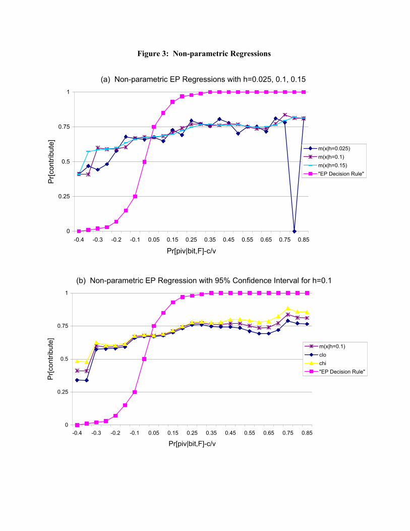
Figure 3: Non-parametric Regressions

(a) Non-parametric EP Regressions with h=0.025, 0.1, 0.15

0

0.25

0.5

0.75

1

-0.4 -0.3 -0.2 -0.1 0.05 0.15 0.25 0.35 0.45 0.55 0.65 0.75 0.85

Pr[piv|bit,F]-c/v

Pr[c

ontri

bute

]

m(x|h=0.025)m(x|h=0.1)m(x|h=0.15)"EP Decision Rule"

(b) Non-parametric EP Regression with 95% Confidence Interval for h=0.1

0

0.25

0.5

0.75

1

-0.4 -0.3 -0.2 -0.1 0.05 0.15 0.25 0.35 0.45 0.55 0.65 0.75 0.85

Pr[piv|bit,F]-c/v

Pr[c

ontri

bute

]

m(x|h=0.1)clochi"EP Decision Rule"