Embed Size (px)
Citation preview
Discrete Mathematics I
Computer Science Tripos, Part 1APaper 1
Natural Sciences Tripos, Part 1A,Computer Science option
Politics, Psychology and Sociology, Part 1,Introduction to Computer Science option
2009–10
Peter Sewell
Computer Laboratory
University of Cambridge
Time-stamp: <2009-11-01 13:25:09 pes20>
c©Peter Sewell 2008, 2009
1
ContentsSyllabus 3
For Supervisors 4
Learning Guide 4
1 Introduction 6
2 Propositional Logic 82.1 The Language of Propositional Logic . . . . . . . . . . . . . . . . . . . . . . . . . . . 92.2 Equational Reasoning . . . . . . . . . . . . . . . . . . . . . . . . . . . . . . . . . . . 15
3 Predicate Logic 183.1 The Language of Predicate Logic . . . . . . . . . . . . . . . . . . . . . . . . . . . . . 19
4 Proof 22
5 Set Theory 355.1 Relations, Graphs, and Orders . . . . . . . . . . . . . . . . . . . . . . . . . . . . . . 41
6 Induction 46
7 Conclusion 49
A Recap: How To Do Proofs 50A.1 How to go about it . . . . . . . . . . . . . . . . . . . . . . . . . . . . . . . . . . . . . 50A.2 And in More Detail... . . . . . . . . . . . . . . . . . . . . . . . . . . . . . . . . . . . 53
A.2.1 Meet the Connectives . . . . . . . . . . . . . . . . . . . . . . . . . . . . . . . 53A.2.2 Equivalences . . . . . . . . . . . . . . . . . . . . . . . . . . . . . . . . . . . . 53A.2.3 How to Prove a Formula . . . . . . . . . . . . . . . . . . . . . . . . . . . . . . 53A.2.4 How to Use a Formula . . . . . . . . . . . . . . . . . . . . . . . . . . . . . . . 56
A.3 An Example . . . . . . . . . . . . . . . . . . . . . . . . . . . . . . . . . . . . . . . . . 56A.3.1 Proving the PL . . . . . . . . . . . . . . . . . . . . . . . . . . . . . . . . . . . 57A.3.2 Using the PL . . . . . . . . . . . . . . . . . . . . . . . . . . . . . . . . . . . . 57
B Exercises 59
Exercise Sheet 1: Propositional Logic 59
Exercise Sheet 2: Predicate Logic 61
Exercise Sheet 3: Structured Proof 62
Exercise Sheet 4: Sets 62
Exercise Sheet 5: Inductive Proof 64
2
Syllabus
Lecturer: Dr P.M. Sewell
No. of lectures: 8
This course is a prerequisite for all theory courses as well as Discrete Mathematics II,Algorithms I, Security (Part IB and Part II), Artificial Intelligence (Part IB and Part II),Information Theory and Coding (Part II).
Aims
This course will develop the intuition for discrete mathematics reasoning involving numbersand sets.
Lectures
• Logic. The languages of propositional and predicate logic and their relationship toinformal statements, truth tables, validity [3 lectures]
• Proof. Proof of predicate logic formulas. [2 lectures]
• Sets. Basic set constructions and relation properties, including equivalence relations,DAGs, pre-, partial and total orders, and functions. [2 lectures]
• Induction. Proof by induction, including proofs about total functional programs overnatural numbers and lists. [1 lecture]
Objectives
On completing the course, students should be able to
• write a clear statement of a problem as a theorem in mathematical notation;
• prove and disprove assertions using a variety of techniques.
Recommended reading
Biggs, N.L. (1989). Discrete mathematics. Oxford University Press.Bornat, R. (2005). Proof and Disproof in Formal Logic. Oxford University Press.Devlin, K. (2003). Sets, functions, and logic: an introduction to abstract mathematics.Chapman and Hall/CRC Mathematics (3rd ed.).Mattson, H.F. Jr (1993). Discrete mathematics. Wiley.Nissanke, N. (1999). Introductory logic and sets for computer scientists. Addison-Wesley.Polya, G. (1980). How to solve it. Penguin.(*) Rosen, K.H. (1999). Discrete mathematics and its applications (6th ed.). McGraw-Hill.(*) Velleman, D. J. (1994). How to prove it (a structured approach). CUP.
3
For Supervisors (and Students too)
The main aim of the course is to enable students to confidently use the language of propo-sitional and predicate logic, and set theory.
We first introduce the language of propositional logic, discussing the relationship to natural-language argument. We define the meaning of formulae with the truth semantics w.r.t. as-sumptions on the propositional variables, and, equivalently, with truth tables. We alsointroduce equational reasoning using tautologies, to make instantiation and reasoning-in-context explicit.
We then introduce quantifiers, again emphasising the intuitive reading of formulae anddefining the truth semantics. We introduce the notions of free and bound variable (but notalpha equivalence).
We do not develop any metatheory, and we treat propositional assumptions, valuationsof variables, and models of atomic predicate symbols all rather informally. There are noturnstiles, but we talk about valid formulae and (briefly) about satisfiable formulae.
We then introduce ‘structured’ proof. This is essentially natural deduction proof, but laidout on the page in roughly the box-and-line style used by Bornat (2005). We don’t give theusual horizontal-line presentation of the rules. The rationale here is to introduce a style ofproof for which one can easily define what is (or is not) a legal proof, but where the prooftext on the page is reasonably close to the normal mathematical ‘informal but rigorous’practice that will be used in most of the rest of the Tripos. We emphasise how to prove andhow to use each connective, and talk about the pragmatics of finding and writing proofs.
The set theory material introduces the basic notions of set, element, union, intersection,powerset, and product, relating to predicates (e.g. relating predicates and set comprehen-sions, and the properties of union to those of disjunction), with some more small exampleproofs. We then define some of the standard properties of relations (reflexive, symmetric,transitive, antisymmetric, acyclic, total) to characterise directed graphs, undirected graphs,equivalence relations, pre-orders, partial orders, and functions). These are illustrated withsimple examples to introduce the concepts, but their properties and uses are not exploredin any depth (for example, we do not define what it means to be an injection or surjection).
Finally, we recall inductive proof over the naturals, making the induction principle explicitin predicate logic, and over lists, talking about inductive proof of simple pure functionalprograms (taking examples from the previous SWEng II notes).
I’d suggest 3 supervisons. A possible schedule might be:
1. After the first 2–3 lectures (on or after Thurs 19 Nov)Example Sheets 1 and 2, covering Propositional and Predicate Logic
2. After the next 3–4 lectures (on or after Thurs 26 Nov)Example Sheets 3 and the first part of 4, covering Structured Proof and Sets
3. After all 8 lectures (on or after Thurs 3 Dec)Example Sheet 4 (the remainder) and 5, covering Inductive Proof
Learning Guide
Notes: These notes include all the slides, but by no means everything that’ll be said inlectures.
Exercises: There are some exercises at the end of the notes. I suggest you do all of them.Most should be rather straightforward; they’re aimed at strengthening your intuition aboutthe concepts and helping you develop quick (but precise) manipulation skills, not to providedeep intellectual challenges. A few may need a bit more thought. Some are taken (or
4

adapted) from Devlin, Rosen, or Velleman. More exercises and examples can be found inany of those.
Tripos questions: This version of the course was new in 2008.
Feedback: Please do complete the on-line feedback form at the end of the course, and letme know during it if you discover errors in the notes or if the pace is too fast or slow.
Errata: A list of any corrections to the notes will be on the course web page.
5
1 Introduction
Discrete Mathematics 1
Computer Science Tripos, Part 1A
Natural Sciences Tripos, Part 1A, Computer Science
Politics, Psychology and Sociology Part 1, Introduction to Computer Science
Peter Sewell
1A, 8 lectures
2009 – 2010
Introduction
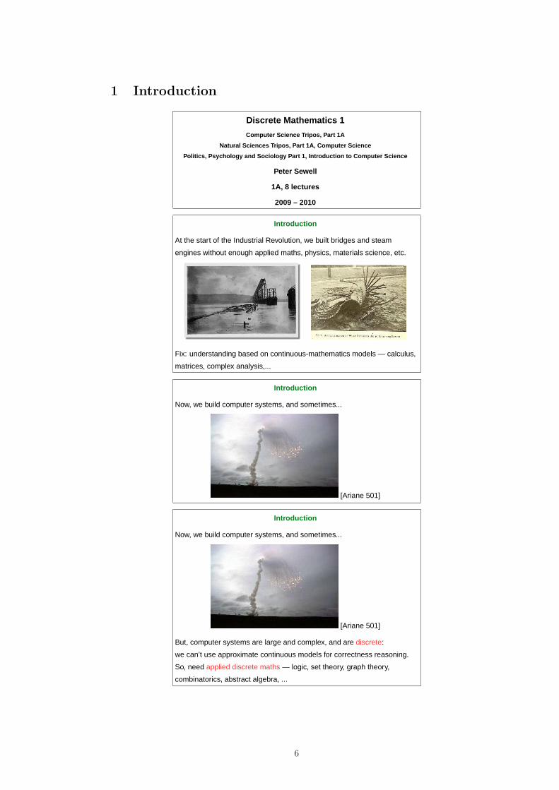
At the start of the Industrial Revolution, we built bridges and steam
engines without enough applied maths, physics, materials science, etc.
Fix: understanding based on continuous-mathematics models — calculus,
matrices, complex analysis,...
Introduction
Now, we build computer systems, and sometimes...
[Ariane 501]
Introduction
Now, we build computer systems, and sometimes...
[Ariane 501]
But, computer systems are large and complex, and are discrete:
we can’t use approximate continuous models for correctness reasoning.
So, need applied discrete maths — logic, set theory, graph theory,
combinatorics, abstract algebra, ...
6
Logic and Set Theory — Pure Mathematics
Origins with the Greeks, 500–350 BC, philosophy and geometry:
Aristotle, Euclid
Formal logic in the 1800s:
De Morgan, Boole, Venn, Peirce, Frege
Set theory, model theory, proof theory; late 1800s and early 1900s:
Cantor, Russell, Hilbert, Zermelo, Frankel, Goedel, Turing, Bourbaki, Gentzen, Tarski
Focus then on the foundations of mathematics — but what was developed
then turns out to be unreasonably effective in Computer Science. This is
the core of the applied maths that we need.
Logic and Set Theory — Applications in Computer Science
• modelling digital circuits (1A Digital Electronics, 1B ECAD)
• proofs about particular algorithms and code (1A Algorithms 1, 1B
Algorithms 2)
• proofs about what is (or is not!) computable and with what complexity
(1B Computation Theory, Complexity Theory)
• proofs about programming languages and type systems (1A Regular
Languages and Finite Automata, 1B Semantics of Programming
Languages, 2 Types)
• foundation of databases (1B Databases)
• automated reasoning and model-checking tools (1B Logic & Proof, 2
Specification & Verification)
Outline
• Propositional Logic
• Predicate Logic
• Sets
• Inductive Proof
Focus on using this material, rather than on metatheoretic study.
More (and more metatheory) in Discrete Maths 2 and in Logic & Proof.
New course last year — feedback welcome.
7
Supervisons
Not rocket science (?), but needs practice to become fluent.
Five example sheets. Many more suitable exercises in the books.
Up to your DoS and supervisor, but I’d suggest 3 supervisons. A possible
schedule might be:
1. After the first 2–3 lectures (on or after Thurs 19 Nov)
Example Sheets 1 and 2, covering Propositional and Predicate Logic
2. After the next 3–4 lectures (on or after Thurs 26 Nov)
Example Sheets 3 and the first part of 4, covering Structured Proof
and Sets
3. After all 8 lectures (on or after Thurs 3 Dec)
Example Sheet 4 (the remainder) and 5, covering Inductive Proof
2 Propositional Logic
Propositional Logic
Propositional Logic
Starting point is informal natural-language argument:
Socrates is a man. All men are mortal. So Socrates is mortal.
Propositional Logic
Starting point is informal natural-language argument:
Socrates is a man. All men are mortal. So Socrates is mortal.
If a person runs barefoot, then his feet hurt. Socrates’ feet hurt.
Therefore, Socrates ran barefoot
It will either rain or snow tomorrow. It’s too warm for snow.
Therefore, it will rain.
8
It will either rain or snow tomorrow. It’s too warm for snow.
Therefore, it will rain.
Either the butler is guilty or the maid is guilty. Either the maid is
guilty or the cook is guilty. Therefore, either the butler is guilty or
the cook is guilty.
It will either rain or snow tomorrow. It’s too warm for snow.
Therefore, it will rain.
Either the framger widget is misfiring or the wrompal mechanism is
out of alignment. I’ve checked the alignment of the wrompal
mechanism, and it’s fine. Therefore, the framger widget is misfiring.
Either the framger widget is misfiring or the wrompal mechanism is
out of alignment. I’ve checked the alignment of the wrompal
mechanism, and it’s fine. Therefore, the framger widget is misfiring.
Either p or q. Not q. Therefore, p
2.1 The Language of Propositional Logic
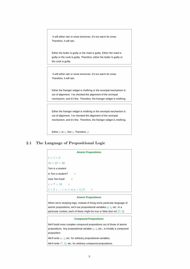
Atomic Propositions
1 + 1 = 2
10 + 10 = 30
Tom is a student
Is Tom a student? ×
Give Tom food! ×
x + 7 = 10 ×
1 + 2 + ... + n = n(n + 1)/2 ×
Atomic Propositions
When we’re studying logic, instead of fixing some particular language of
atomic propositions, we’ll use propositional variables p, q, etc. In a
particular context, each of these might be true or false (but not 21.5).
Compound Propositions
We’ll build more complex compound propositions out of those of atomic
propositions. Any propositional variable p, q, etc., is trivially a compound
proposition.
We’ll write p, q , etc. for arbitrary propositional variables.
We’ll write P , Q , etc. for arbitrary compound propositions.
9
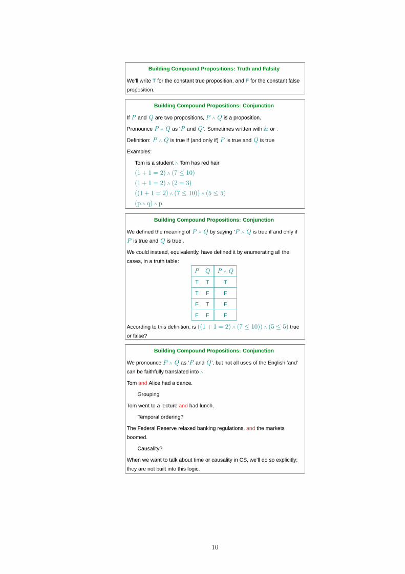
Building Compound Propositions: Truth and Falsity
We’ll write T for the constant true proposition, and F for the constant false
proposition.
Building Compound Propositions: Conjunction
If P and Q are two propositions, P ∧ Q is a proposition.
Pronounce P ∧ Q as ‘P and Q ’. Sometimes written with & or .
Definition: P ∧ Q is true if (and only if) P is true and Q is true
Examples:
Tom is a student ∧ Tom has red hair
(1 + 1 = 2) ∧ (7 ≤ 10)
(1 + 1 = 2) ∧ (2 = 3)
((1 + 1 = 2) ∧ (7 ≤ 10)) ∧ (5 ≤ 5)
(p ∧ q) ∧ p
Building Compound Propositions: Conjunction
We defined the meaning of P ∧ Q by saying ‘P ∧ Q is true if and only if
P is true and Q is true’.
We could instead, equivalently, have defined it by enumerating all the
cases, in a truth table:
P Q P ∧ Q
T T T
T F F
F T F
F F F
According to this definition, is ((1 + 1 = 2) ∧ (7 ≤ 10)) ∧ (5 ≤ 5) true
or false?
Building Compound Propositions: Conjunction
We pronounce P ∧ Q as ‘P and Q ’, but not all uses of the English ‘and’
can be faithfully translated into ∧.
Tom and Alice had a dance.
Grouping
Tom went to a lecture and had lunch.
Temporal ordering?
The Federal Reserve relaxed banking regulations, and the markets
boomed.
Causality?
When we want to talk about time or causality in CS, we’ll do so explicitly;
they are not built into this logic.
10
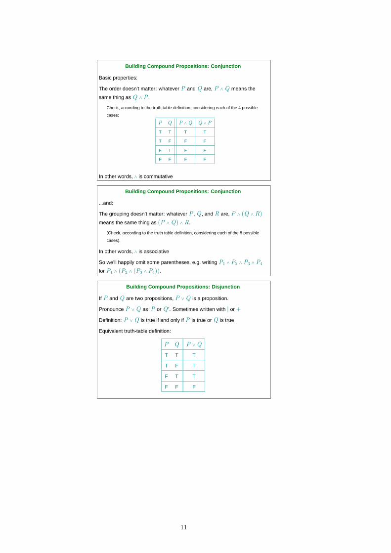
Building Compound Propositions: Conjunction
Basic properties:
The order doesn’t matter: whatever P and Q are, P ∧ Q means the
same thing as Q ∧ P .
Check, according to the truth table definition, considering each of the 4 possible
cases:
P Q P ∧ Q Q ∧ P
T T T T
T F F F
F T F F
F F F F
In other words, ∧ is commutative
Building Compound Propositions: Conjunction
...and:
The grouping doesn’t matter: whatever P , Q , and R are, P ∧ (Q ∧ R)
means the same thing as (P ∧ Q) ∧ R.
(Check, according to the truth table definition, considering each of the 8 possible
cases).
In other words, ∧ is associative
So we’ll happily omit some parentheses, e.g. writing P1 ∧ P2 ∧ P3 ∧ P4
for P1 ∧ (P2 ∧ (P3 ∧ P4)).
Building Compound Propositions: Disjunction
If P and Q are two propositions, P ∨ Q is a proposition.
Pronounce P ∨ Q as ‘P or Q ’. Sometimes written with | or +
Definition: P ∨ Q is true if and only if P is true or Q is true
Equivalent truth-table definition:
P Q P ∨ Q
T T T
T F T
F T T
F F F
11

Building Compound Propositions: Disjunction
You can see from that truth table that ∨ is an inclusive or: P ∨ Q if at least
one of P and Q .
(2 + 2 = 4) ∨ (3 + 3 = 6) is true
(2 + 2 = 4) ∨ (3 + 3 = 7) is true
The English ‘or’ is sometimes an exclusive or: P xor Q if exactly one of
P and Q . ‘Fluffy is either a rabbit or a cat.’
P Q P ∨ Q P xor Q
T T T F
T F T T
F T T T
F F F F
(we won’t use xor so much).
Building Compound Propositions: Disjunction
Basic Properties
∨ is also commutative and associative:
P ∨ Q and Q ∨ P have the same meaning
P ∨ (Q ∨ R) and (P ∨ Q) ∨ R have the same meaning
∧ distributes over ∨:
P ∧ (Q ∨ R) and (P ∧ Q) ∨ (P ∧ R) have the same meaning
‘P and either Q or R’ ‘either (P and Q ) or (P and R)’
and the other way round: ∨ distributes over ∧
P ∨ (Q ∧ R) and (P ∨ Q) ∧ (P ∨ R) have the same meaning
When we mix ∧ and ∨, we take care with the parentheses!
Building Compound Propositions: Negation
If P is some proposition, ¬P is a proposition.
Pronounce ¬P as ‘not P ’. Sometimes written as∼P or P
Definition: ¬P is true if and only if P is false
Equivalent truth-table definition:
P ¬P
T F
F T
12
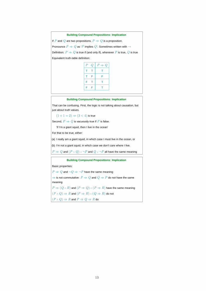
Building Compound Propositions: Implication
If P and Q are two propositions, P ⇒ Q is a proposition.
Pronounce P ⇒ Q as ‘P implies Q ’. Sometimes written with→
Definition: P ⇒ Q is true if (and only if), whenever P is true, Q is true
Equivalent truth-table definition:
P Q P ⇒ Q
T T T
T F F
F T T
F F T
Building Compound Propositions: Implication
That can be confusing. First, the logic is not talking about causation, but
just about truth values.
(1 + 1 = 2)⇒ (3 < 4) is true
Second, P ⇒ Q is vacuously true if P is false.
‘If I’m a giant squid, then I live in the ocean’
For that to be true, either:
(a) I really am a giant squid, in which case I must live in the ocean, or
(b) I’m not a giant squid, in which case we don’t care where I live.
P ⇒ Q and (P ∧ Q) ∨ ¬P and Q ∨ ¬P all have the same meaning
Building Compound Propositions: Implication
Basic properties:
P ⇒ Q and ¬Q ⇒ ¬P have the same meaning
⇒ is not commutative: P ⇒ Q and Q ⇒ P do not have the same
meaning
P ⇒ (Q ∧ R) and (P ⇒ Q) ∧ (P ⇒ R) have the same meaning
(P ∧ Q)⇒ R and (P ⇒ R) ∧ (Q ⇒ R) do not
(P ∧ Q)⇒ R and P ⇒ Q ⇒ R do
13
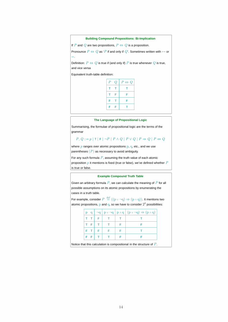
Building Compound Propositions: Bi-Implication
If P and Q are two propositions, P ⇔ Q is a proposition.
Pronounce P ⇔ Q as ‘P if and only if Q ’. Sometimes written with↔ or
=.
Definition: P ⇔ Q is true if (and only if) P is true whenever Q is true,
and vice versa
Equivalent truth-table definition:
P Q P ⇔ Q
T T T
T F F
F T F
F F T
The Language of Propositional Logic
Summarising, the formulae of propositional logic are the terms of the
grammar
P ,Q ::= p | T | F | ¬P | P ∧Q | P ∨Q | P ⇒ Q | P ⇔ Q
where p ranges over atomic propositions p, q, etc., and we use
parentheses (P) as necessary to avoid ambiguity.
For any such formula P , assuming the truth value of each atomic
proposition p it mentions is fixed (true or false), we’ve defined whether P
is true or false.
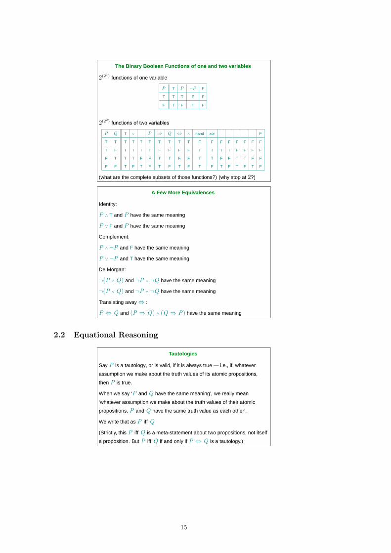
Example Compound Truth Table
Given an arbitrary formula P , we can calculate the meaning of P for all
possible assumptions on its atomic propositions by enumerating the
cases in a truth table.
For example, consider Pdef= ((p ∨ ¬q)⇒ (p ∧ q)). It mentions two
atomic propositions, p and q, so we have to consider 22 possibilities:
p q ¬q p ∨ ¬q p ∧ q (p ∨ ¬q)⇒ (p ∧ q)
T T F T T T
T F T T F F
F T F F F T
F F T T F F
Notice that this calculation is compositional in the structure of P .
14
The Binary Boolean Functions of one and two variables
2(21) functions of one variable
P T P ¬P F
T T T F F
F T F T F
2(22) functions of two variables
P Q T ∨ P ⇒ Q ⇔ ∧ nand xor F
T T T T T T T T T T F F F F F F F F
T F T T T T F F F F T T T T F F F F
F T T T F F T T F F T T F F T T F F
F F T F T F T F T F T F T F T F T F
(what are the complete subsets of those functions?) (why stop at 2?)
A Few More Equivalences
Identity:
P ∧ T and P have the same meaning
P ∨ F and P have the same meaning
Complement:
P ∧ ¬P and F have the same meaning
P ∨ ¬P and T have the same meaning
De Morgan:
¬(P ∧ Q) and ¬P ∨ ¬Q have the same meaning
¬(P ∨ Q) and ¬P ∧ ¬Q have the same meaning
Translating away⇔ :
P ⇔ Q and (P ⇒ Q) ∧ (Q ⇒ P) have the same meaning
2.2 Equational Reasoning
Tautologies
Say P is a tautology, or is valid, if it is always true — i.e., if, whatever
assumption we make about the truth values of its atomic propositions,
then P is true.
When we say ‘P and Q have the same meaning’, we really mean
‘whatever assumption we make about the truth values of their atomic
propositions, P and Q have the same truth value as each other’.
We write that as P iff Q
(Strictly, this P iff Q is a meta-statement about two propositions, not itself
a proposition. But P iff Q if and only if P ⇔ Q is a tautology.)
15
Equational Reasoning
Tautologies are really useful — because they can be used anywhere.
In more detail, this P iff Q is a proper notion of equality. You can see
from its definition that
• it’s reflexive, i.e., for any P , we have P iff P
• it’s symmetric, i.e., if P iff Q then Q iff P
• it’s transitive, i.e., if P iff Q and Q iff R then P iff R
Moreover, if P iff Q then we can replace a subformula P by Q in any
context, without affecting the meaning of the whole thing. For example,
if P iff Q then P ∧ R iff Q ∧ R, R ∧ P iff R ∧ Q , ¬P iff ¬Q , etc.
Equational Reasoning
Now we’re in business: we can do equational reasoning, replacing equal
subformulae by equal subformulae, just as you do in normal algebraic
manipulation (where you’d use 2 + 2 = 4 without thinking).
This complements direct verification using truth tables — sometimes
that’s more convenient, and sometimes this is. Later, we’ll see a third
option — structured proof.
Some Collected Tautologies, for Reference
For any propositions P , Q , and R
Commutativity:
P ∧ Q iff Q ∧ P (and-comm)
P ∨ Q iff Q ∨ P (or-comm)
Associativity:
P ∧ (Q ∧ R) iff (P ∧ Q) ∧ R (and-assoc)
P ∨ (Q ∨ R) iff (P ∨ Q) ∨ R (or-assoc)
Distributivity:
P ∧ (Q ∨ R) iff (P ∧ Q) ∨ (P ∧ R) (and-or-dist)
P ∨ (Q ∧ R) iff (P ∨ Q) ∧ (P ∨ R) (or-and-dist)
Identity:
P ∧ T iff P (and-id)
P ∨ F iff P (or-id)
Unit:
P ∧ F iff F (and-unit)
P ∨ T iff T (or-unit)
Complement:
P ∧ ¬P iff F (and-comp)
P ∨ ¬P iff T (or-comp)
De Morgan:
¬(P ∧ Q) iff ¬P ∨ ¬Q (and-DM)
¬(P ∨ Q) iff ¬P ∧ ¬Q (or-DM)
Defn:
P ⇒ Q iff Q ∨ ¬P (imp)
P ⇔ Q = (P ⇒ Q) ∧ (Q ⇒ P) (bi)
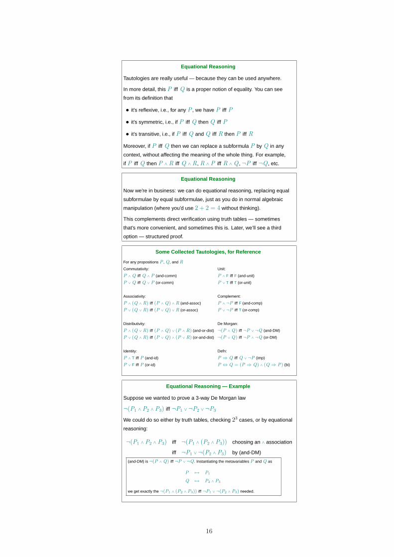
Equational Reasoning — Example
Suppose we wanted to prove a 3-way De Morgan law
¬(P1 ∧ P2 ∧ P3) iff ¬P1 ∨ ¬P2 ∨ ¬P3
We could do so either by truth tables, checking 23 cases, or by equational
reasoning:
¬(P1 ∧ P2 ∧ P3) iff ¬(P1 ∧ (P2 ∧ P3)) choosing an ∧ association
iff ¬P1 ∨ ¬(P2 ∧ P3) by (and-DM)
(and-DM) is ¬(P ∧ Q) iff ¬P ∨ ¬Q . Instantiating the metavariables P and Q as
P 7→ P1
Q 7→ P2 ∧ P3
we get exactly the ¬(P1 ∧ (P2 ∧ P3)) iff ¬P1 ∨ ¬(P2 ∧ P3) needed.
16
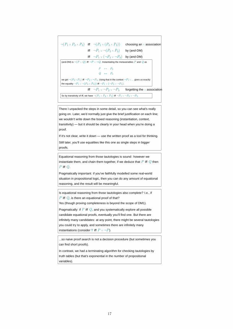
¬(P1 ∧ P2 ∧ P3) iff ¬(P1 ∧ (P2 ∧ P3)) choosing an ∧ association
iff ¬P1 ∨ ¬(P2 ∧ P3) by (and-DM)
iff ¬P1 ∨ (¬P2 ∨ ¬P3) by (and-DM)
(and-DM) is ¬(P ∧ Q) iff ¬P ∨ ¬Q . Instantiating the metavariables P and Q as
P 7→ P2
Q 7→ P3
we get ¬(P2 ∧P3) iff ¬P2 ∨¬P3. Using that in the context ¬P1 ∨ ... gives us exactly
the equality ¬P1 ∨ ¬(P2 ∧ P3)) iff ¬P1 ∨ (¬P2 ∨ ¬P3).
iff ¬P1 ∨ ¬P2 ∨ ¬P3 forgetting the ∨ association
So by transitivity of iff, we have ¬(P1 ∧ P2 ∧ P3) iff ¬P1 ∨ ¬P2 ∨ ¬P3
There I unpacked the steps in some detail, so you can see what’s really
going on. Later, we’d normally just give the brief justification on each line;
we wouldn’t write down the boxed reasoning (instantiation, context,
transitivity) — but it should be clearly in your head when you’re doing a
proof.
If it’s not clear, write it down — use the written proof as a tool for thinking.
Still later, you’ll use equalities like this one as single steps in bigger
proofs.
Equational reasoning from those tautologies is sound : however we
instantiate them, and chain them together, if we deduce that P iff Q then
P iff Q .
Pragmatically important: if you’ve faithfully modelled some real-world
situation in propositional logic, then you can do any amount of equational
reasoning, and the result will be meaningful.
Is equational reasoning from those tautologies also complete? I.e., if
P iff Q , is there an equational proof of that?
Yes (though proving completeness is beyond the scope of DM1).
Pragmatically: if P iff Q , and you systematically explore all possible
candidate equational proofs, eventually you’ll find one. But there are
infinitely many candidates: at any point, there might be several tautologies
you could try to apply, and sometimes there are infinitely many
instantiations (consider T iff P ∨ ¬P ).
...so naive proof search is not a decision procedure (but sometimes you
can find short proofs).
In contrast, we had a terminating algorithm for checking tautologies by
truth tables (but that’s exponential in the number of propositional
variables).
17
Satisfiability
Recall P is a tautology, or is valid, if it is always true — i.e., if, whatever
assumption we make about the truth values of its atomic propositions,
then P is true.
Say P is a satisfiable if, under some assumption about the truth values of
its atomic propositions, P is true.
p ∧ ¬q satisfiable (true under the assumption p 7→ T, q 7→ F)
p ∧ ¬p unsatisfiable (not true under p 7→ T or p 7→ F)
P unsatisfiable iff ¬P valid
Object, Meta, Meta-Meta,...
We’re taking care to distinguish the connectives of the object language
(propositional logic) that we’re studying, and the informal mathematics
and English that we’re using to talk about it (our meta-language).
For now, we adopt a simple discipline: the former in symbols, the latter in
words.
Later, you’ll use logic to talk about logic.
Application: Combinational Circuits
Use T and F to represent high and low voltage values on a wire.
Logic gates (AND, OR, NAND, etc.) compute propositional functions of
their inputs.
Notation: T, F, ∧, ∨, ¬ vs 0, 1, ., +,
SAT solvers: compute satisfiability of formulae with 10 000’s of
propositional variables.
3 Predicate Logic
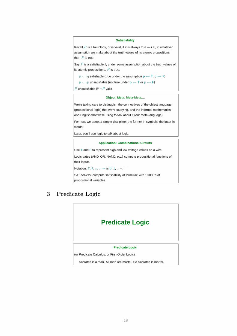
Predicate Logic
Predicate Logic
(or Predicate Calculus, or First-Order Logic)
Socrates is a man. All men are mortal. So Socrates is mortal.
18
Predicate Logic
(or Predicate Calculus, or First-Order Logic)
Socrates is a man. All men are mortal. So Socrates is mortal.
Can we formalise in propositional logic?
Write p for Socrates is a man
Write q for Socrates is mortal
p p⇒ q q
?
Predicate Logic
Often, we want to talk about properties of things, not just atomic
propositions.
All lions are fierce.
Some lions do not drink coffee.
Therefore, some fierce creatures do not drink coffee.
[Lewis Carroll, 1886]
Let x range over creatures. Write L(x ) for ‘x is a lion’. Write C(x ) for ‘x
drinks coffee’. Write F(x ) for ‘x is fierce’.
∀ x .L(x )⇒ F(x )
∃ x .L(x ) ∧ ¬C(x )
∃ x .F(x ) ∧ ¬C(x )
3.1 The Language of Predicate Logic
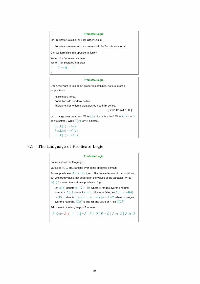
Predicate Logic
So, we extend the language.
Variables x , y , etc., ranging over some specified domain.
Atomic predicates A(x ), B(x ), etc., like the earlier atomic propositions,
but with truth values that depend on the values of the variables. Write
A(x ) for an arbitrary atomic predicate. E.g.:
Let A(x ) denote x + 7 = 10, where x ranges over the natural
numbers. A(x ) is true if x = 3, otherwise false, so A(3) ∧ ¬A(4)
Let B(n) denote 1 + 2 + ... + n = n(n + 1)/2, where n ranges
over the naturals. B(n) is true for any value of n , so B(27).
Add these to the language of formulae:
P ,Q ::=A(x ) | T | F | ¬P | P ∧Q | P ∨Q | P ⇒ Q | P ⇔ Q
19
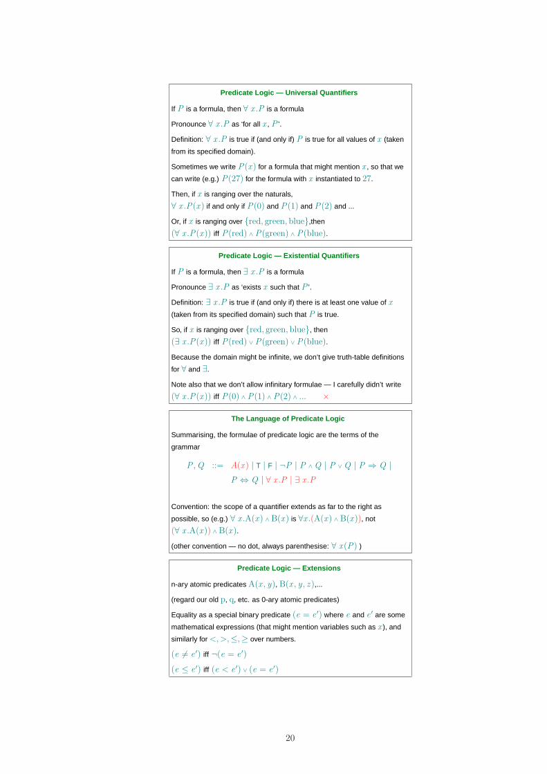
Predicate Logic — Universal Quantifiers
If P is a formula, then ∀ x .P is a formula
Pronounce ∀ x .P as ‘for all x , P ’.
Definition: ∀ x .P is true if (and only if) P is true for all values of x (taken
from its specified domain).
Sometimes we write P(x ) for a formula that might mention x , so that we
can write (e.g.) P(27) for the formula with x instantiated to 27.
Then, if x is ranging over the naturals,
∀ x .P(x ) if and only if P(0) and P(1) and P(2) and ...
Or, if x is ranging over {red, green, blue},then
(∀ x .P(x )) iff P(red) ∧ P(green) ∧ P(blue).
Predicate Logic — Existential Quantifiers
If P is a formula, then ∃ x .P is a formula
Pronounce ∃ x .P as ‘exists x such that P ’.
Definition: ∃ x .P is true if (and only if) there is at least one value of x
(taken from its specified domain) such that P is true.
So, if x is ranging over {red, green, blue}, then
(∃ x .P(x )) iff P(red) ∨ P(green) ∨ P(blue).
Because the domain might be infinite, we don’t give truth-table definitions
for ∀ and ∃.
Note also that we don’t allow infinitary formulae — I carefully didn’t write
(∀ x .P(x )) iff P(0) ∧ P(1) ∧ P(2) ∧ ... ×
The Language of Predicate Logic
Summarising, the formulae of predicate logic are the terms of the
grammar
P ,Q ::= A(x ) | T | F | ¬P | P ∧ Q | P ∨ Q | P ⇒ Q |
P ⇔ Q | ∀ x .P | ∃ x .P
Convention: the scope of a quantifier extends as far to the right as
possible, so (e.g.) ∀ x .A(x ) ∧ B(x ) is ∀x .(A(x ) ∧ B(x )), not
(∀ x .A(x )) ∧ B(x ).
(other convention — no dot, always parenthesise: ∀ x (P) )
Predicate Logic — Extensions
n-ary atomic predicates A(x , y), B(x , y , z ),...
(regard our old p, q, etc. as 0-ary atomic predicates)
Equality as a special binary predicate (e = e ′) where e and e ′ are some
mathematical expressions (that might mention variables such as x ), and
similarly for <,>,≤,≥ over numbers.
(e 6= e ′) iff ¬(e = e ′)
(e ≤ e ′) iff (e < e ′) ∨ (e = e ′)
20
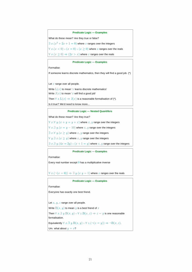
Predicate Logic — Examples
What do these mean? Are they true or false?
∃ x .(x 2 + 2x + 1 = 0) where x ranges over the integers
∀ x .(x < 0) ∨ (x = 0) ∨ (x ≥ 0) where x ranges over the reals
∀ x .(x ≥ 0)⇒ (2x > x ) where x ranges over the reals
Predicate Logic — Examples
Formalise:
If someone learns discrete mathematics, then they will find a good job. (*)
Let x range over all people.
Write L(x ) to mean ‘x learns discrete mathematics’
Write J(x ) to mean ‘x will find a good job’
Then ∀ x .L(x )⇒ J(x ) is a reasonable formalisation of (*).
Is it true? We’d need to know more...
Predicate Logic — Nested Quantifers
What do these mean? Are they true?
∀ x .∀ y .(x + y = y + x ) where x , y range over the integers
∀ x .∃ y .(x = y − 10) where x , y range over the integers
∃ x .∀ y .(x ≥ y) where x , y range over the integers
∀ y .∃ x .(x ≥ y) where x , y range over the integers
∃ x .∃ y .(4x = 2y) ∧ (x + 1 = y) where x , y range over the integers
Predicate Logic — Examples
Formalise:
Every real number except 0 has a multiplicative inverse
∀ x .(¬(x = 0))⇒ ∃ y .(x y = 1) where x ranges over the reals
Predicate Logic — Examples
Formalise:
Everyone has exactly one best friend.
Let x , y , z range over all people.
Write B(x , y) to mean y is a best friend of x
Then ∀ x .∃ y .B(x , y) ∧ ∀ z .B(x , z )⇒ z = y is one reasonable
formalisation.
Equivalently ∀ x .∃ y .B(x , y) ∧ ∀ z .(¬(z = y))⇒ ¬B(x , z ).
Um. what about y = x?
21
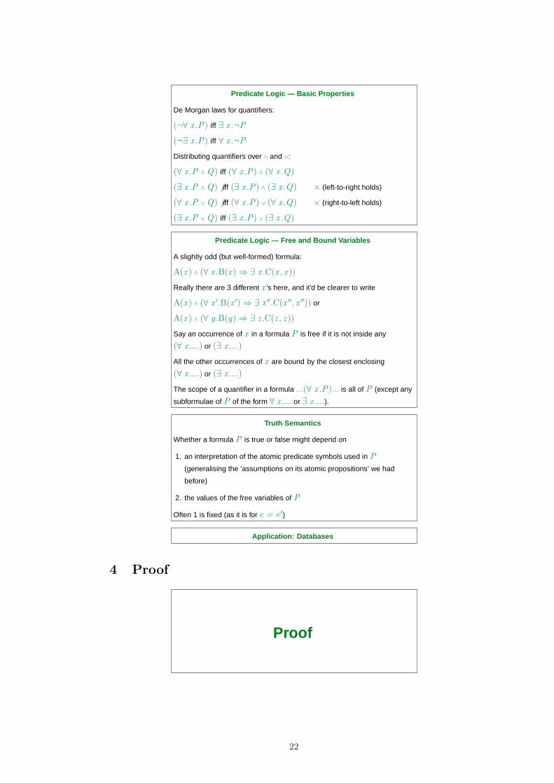
Predicate Logic — Basic Properties
De Morgan laws for quantifiers:
(¬∀ x .P) iff ∃ x .¬P
(¬∃ x .P) iff ∀ x .¬P
Distributing quantifiers over ∧ and ∨:
(∀ x .P ∧ Q) iff (∀ x .P) ∧ (∀ x .Q)
(∃ x .P ∧ Q) 6 iff (∃ x .P) ∧ (∃ x .Q) × (left-to-right holds)
(∀ x .P ∨ Q) 6 iff (∀ x .P) ∨ (∀ x .Q) × (right-to-left holds)
(∃ x .P ∨ Q) iff (∃ x .P) ∨ (∃ x .Q)
Predicate Logic — Free and Bound Variables
A slightly odd (but well-formed) formula:
A(x ) ∧ (∀ x .B(x )⇒ ∃ x .C(x , x ))
Really there are 3 different x ’s here, and it’d be clearer to write
A(x ) ∧ (∀ x ′.B(x ′)⇒ ∃ x ′′.C(x ′′, x ′′)) or
A(x ) ∧ (∀ y .B(y)⇒ ∃ z .C(z , z ))
Say an occurrence of x in a formula P is free if it is not inside any
(∀ x ....) or (∃ x ....)
All the other occurrences of x are bound by the closest enclosing
(∀ x ....) or (∃ x ....)
The scope of a quantifier in a formula ...(∀ x .P)... is all of P (except any
subformulae of P of the form ∀ x .... or ∃ x ....).
Truth Semantics
Whether a formula P is true or false might depend on
1. an interpretation of the atomic predicate symbols used in P
(generalising the ‘assumptions on its atomic propositions’ we had
before)
2. the values of the free variables of P
Often 1 is fixed (as it is for e = e ′)
Application: Databases
4 Proof
Proof
22
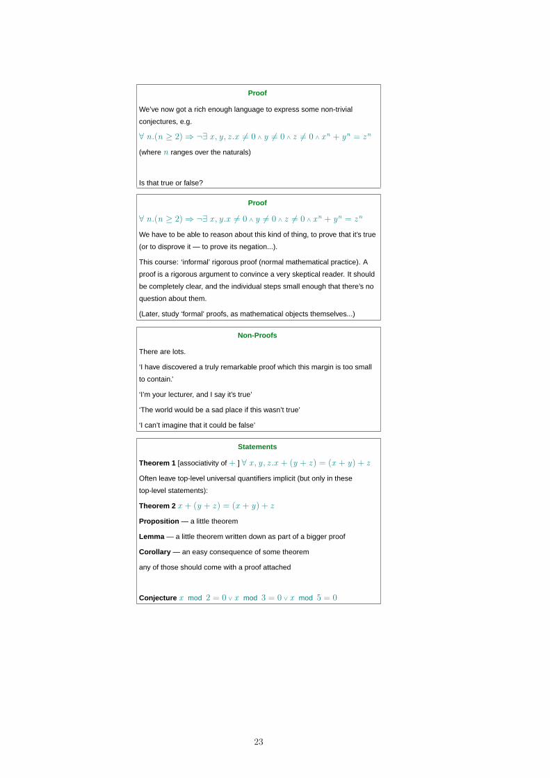
Proof
We’ve now got a rich enough language to express some non-trivial
conjectures, e.g.
∀ n.(n ≥ 2)⇒ ¬∃ x , y , z .x 6= 0 ∧ y 6= 0 ∧ z 6= 0 ∧ x n + yn = z n
(where n ranges over the naturals)
Is that true or false?
Proof
∀ n.(n ≥ 2)⇒ ¬∃ x , y .x 6= 0 ∧ y 6= 0 ∧ z 6= 0 ∧ x n + yn = z n
We have to be able to reason about this kind of thing, to prove that it’s true
(or to disprove it — to prove its negation...).
This course: ‘informal’ rigorous proof (normal mathematical practice). A
proof is a rigorous argument to convince a very skeptical reader. It should
be completely clear, and the individual steps small enough that there’s no
question about them.
(Later, study ‘formal’ proofs, as mathematical objects themselves...)
Non-Proofs
There are lots.
‘I have discovered a truly remarkable proof which this margin is too small
to contain.’
‘I’m your lecturer, and I say it’s true’
‘The world would be a sad place if this wasn’t true’
‘I can’t imagine that it could be false’
Statements
Theorem 1 [associativity of + ] ∀ x , y , z .x + (y + z ) = (x + y) + z
Often leave top-level universal quantifiers implicit (but only in these
top-level statements):
Theorem 2 x + (y + z ) = (x + y) + z
Proposition — a little theorem
Lemma — a little theorem written down as part of a bigger proof
Corollary — an easy consequence of some theorem
any of those should come with a proof attached
Conjecture x mod 2 = 0 ∨ x mod 3 = 0 ∨ x mod 5 = 0
23
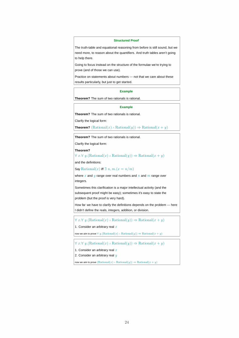
Structured Proof
The truth-table and equational reasoning from before is still sound, but we
need more, to reason about the quantifiers. And truth tables aren’t going
to help there.
Going to focus instead on the structure of the formulae we’re trying to
prove (and of those we can use).
Practice on statements about numbers — not that we care about these
results particularly, but just to get started.
Example
Theorem? The sum of two rationals is rational.
Example
Theorem? The sum of two rationals is rational.
Clarify the logical form:
Theorem? (Rational(x ) ∧ Rational(y))⇒ Rational(x + y)
Theorem? The sum of two rationals is rational.
Clarify the logical form:
Theorem?
∀ x .∀ y .(Rational(x ) ∧ Rational(y))⇒ Rational(x + y)
and the definitions:
Say Rational(x ) iff ∃ n,m.(x = n/m)
where x and y range over real numbers and n and m range over
integers.
Sometimes this clarification is a major intellectual activity (and the
subsequent proof might be easy); sometimes it’s easy to state the
problem (but the proof is very hard).
How far we have to clarify the definitions depends on the problem — here
I didn’t define the reals, integers, addition, or division.
∀ x .∀ y .(Rational(x ) ∧ Rational(y))⇒ Rational(x + y)
1. Consider an arbitrary real x
now we aim to prove ∀ y .(Rational(x ) ∧ Rational(y)) ⇒ Rational(x + y)
∀ x .∀ y .(Rational(x ) ∧ Rational(y))⇒ Rational(x + y)
1. Consider an arbitrary real x
2. Consider an arbitrary real y
now we aim to prove (Rational(x ) ∧ Rational(y)) ⇒ Rational(x + y)
24
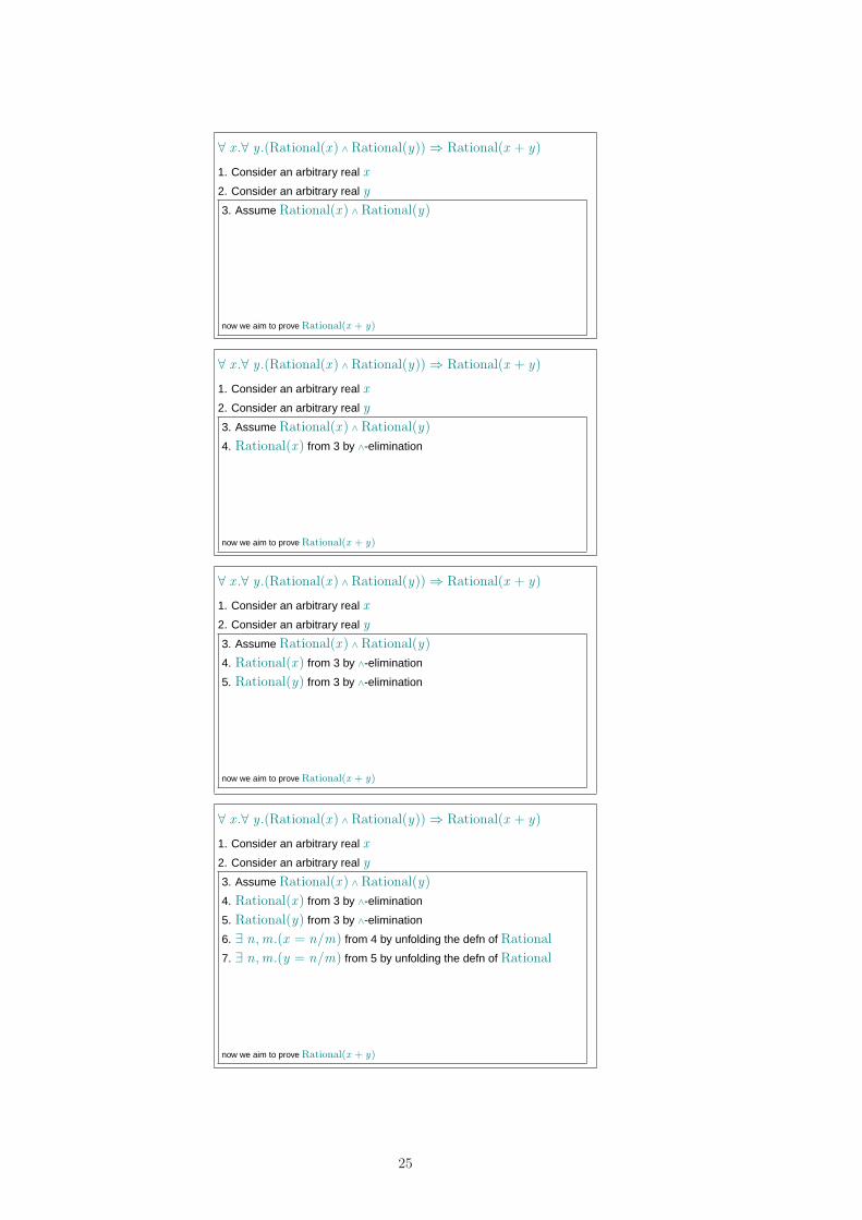
∀ x .∀ y .(Rational(x ) ∧ Rational(y))⇒ Rational(x + y)
1. Consider an arbitrary real x
2. Consider an arbitrary real y
3. Assume Rational(x ) ∧ Rational(y)
now we aim to prove Rational(x + y)
∀ x .∀ y .(Rational(x ) ∧ Rational(y))⇒ Rational(x + y)
1. Consider an arbitrary real x
2. Consider an arbitrary real y
3. Assume Rational(x ) ∧ Rational(y)
4. Rational(x ) from 3 by ∧-elimination
now we aim to prove Rational(x + y)
∀ x .∀ y .(Rational(x ) ∧ Rational(y))⇒ Rational(x + y)
1. Consider an arbitrary real x
2. Consider an arbitrary real y
3. Assume Rational(x ) ∧ Rational(y)
4. Rational(x ) from 3 by ∧-elimination
5. Rational(y) from 3 by ∧-elimination
now we aim to prove Rational(x + y)
∀ x .∀ y .(Rational(x ) ∧ Rational(y))⇒ Rational(x + y)
1. Consider an arbitrary real x
2. Consider an arbitrary real y
3. Assume Rational(x ) ∧ Rational(y)
4. Rational(x ) from 3 by ∧-elimination
5. Rational(y) from 3 by ∧-elimination
6. ∃ n,m.(x = n/m) from 4 by unfolding the defn of Rational
7. ∃ n,m.(y = n/m) from 5 by unfolding the defn of Rational
now we aim to prove Rational(x + y)
25
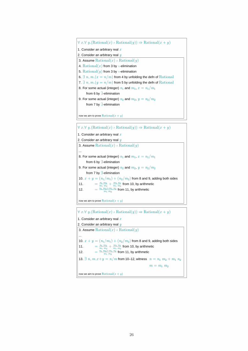
∀ x .∀ y .(Rational(x ) ∧ Rational(y))⇒ Rational(x + y)
1. Consider an arbitrary real x
2. Consider an arbitrary real y
3. Assume Rational(x ) ∧ Rational(y)
4. Rational(x ) from 3 by ∧-elimination
5. Rational(y) from 3 by ∧-elimination
6. ∃ n,m.(x = n/m) from 4 by unfolding the defn of Rational
7. ∃ n,m.(y = n/m) from 5 by unfolding the defn of Rational
8. For some actual (integer) n1 and m1, x = n1/m1
from 6 by ∃-elimination
9. For some actual (integer) n2 and m2, y = n2/m2
from 7 by ∃-elimination
now we aim to prove Rational(x + y)
∀ x .∀ y .(Rational(x ) ∧ Rational(y))⇒ Rational(x + y)
1. Consider an arbitrary real x
2. Consider an arbitrary real y
3. Assume Rational(x ) ∧ Rational(y)
...
8. For some actual (integer) n1 and m1, x = n1/m1
from 6 by ∃-elimination
9. For some actual (integer) n2 and m2, y = n2/m2
from 7 by ∃-elimination
10. x + y = (n1/m1) + (n2/m2) from 8 and 9, adding both sides
11. = n1 m2
m1 m2+ m1 n2
m1 m2from 10, by arithmetic
12. = n1 m2+m1 n2
m1 m2from 11, by arithmetic
now we aim to prove Rational(x + y)
∀ x .∀ y .(Rational(x ) ∧ Rational(y))⇒ Rational(x + y)
1. Consider an arbitrary real x
2. Consider an arbitrary real y
3. Assume Rational(x ) ∧ Rational(y)
...
10. x + y = (n1/m1) + (n2/m2) from 8 and 9, adding both sides
11. = n1 m2
m1 m2+ m1 n2
m1 m2from 10, by arithmetic
12. = n1 m2+m1 n2
m1 m2from 11, by arithmetic
13. ∃ n,m.x+y = n/m from 10–12, witness n = n1 m2 + m1 n2
m = m1 m2
now we aim to prove Rational(x + y)
26
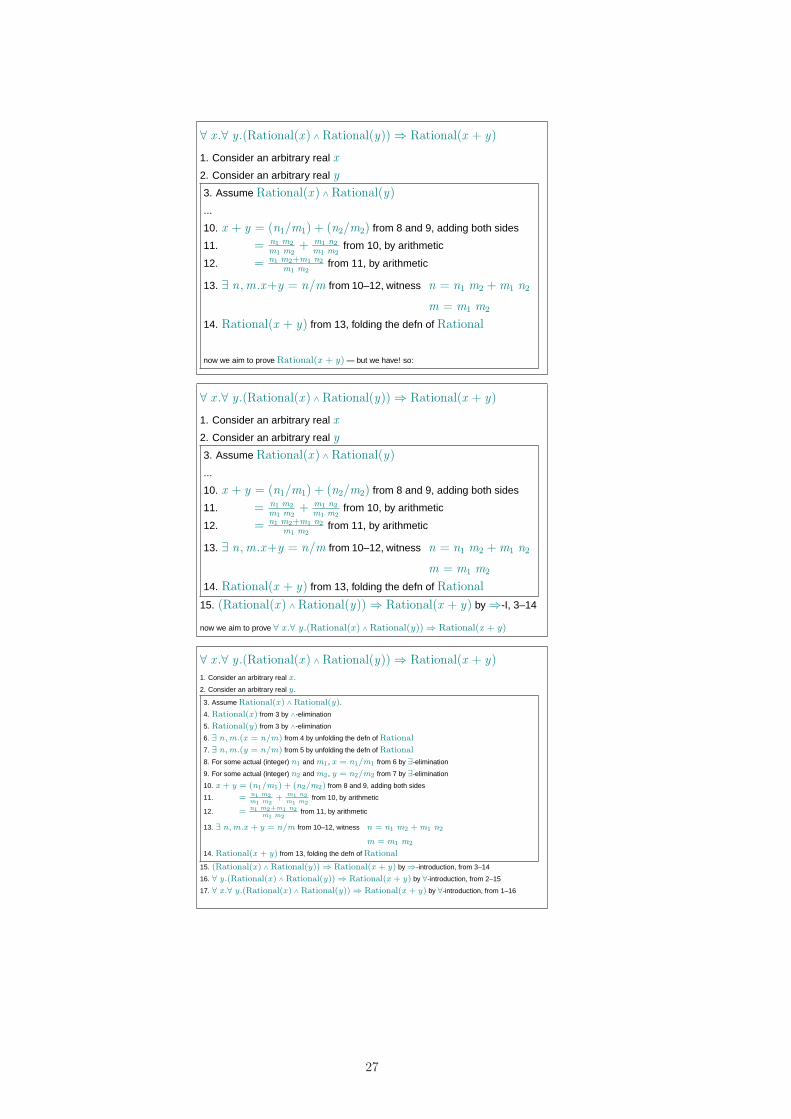
∀ x .∀ y .(Rational(x ) ∧ Rational(y))⇒ Rational(x + y)
1. Consider an arbitrary real x
2. Consider an arbitrary real y
3. Assume Rational(x ) ∧ Rational(y)
...
10. x + y = (n1/m1) + (n2/m2) from 8 and 9, adding both sides
11. = n1 m2
m1 m2+ m1 n2
m1 m2from 10, by arithmetic
12. = n1 m2+m1 n2
m1 m2from 11, by arithmetic
13. ∃ n,m.x+y = n/m from 10–12, witness n = n1 m2 + m1 n2
m = m1 m2
14. Rational(x + y) from 13, folding the defn of Rational
now we aim to prove Rational(x + y) — but we have! so:
∀ x .∀ y .(Rational(x ) ∧ Rational(y))⇒ Rational(x + y)
1. Consider an arbitrary real x
2. Consider an arbitrary real y
3. Assume Rational(x ) ∧ Rational(y)
...
10. x + y = (n1/m1) + (n2/m2) from 8 and 9, adding both sides
11. = n1 m2
m1 m2+ m1 n2
m1 m2from 10, by arithmetic
12. = n1 m2+m1 n2
m1 m2from 11, by arithmetic
13. ∃ n,m.x+y = n/m from 10–12, witness n = n1 m2 + m1 n2
m = m1 m2
14. Rational(x + y) from 13, folding the defn of Rational
15. (Rational(x ) ∧ Rational(y))⇒ Rational(x + y) by⇒-I, 3–14
now we aim to prove ∀ x .∀ y .(Rational(x ) ∧ Rational(y)) ⇒ Rational(x + y)
∀ x .∀ y .(Rational(x ) ∧ Rational(y))⇒ Rational(x + y)
1. Consider an arbitrary real x .
2. Consider an arbitrary real y .
3. Assume Rational(x) ∧ Rational(y).
4. Rational(x) from 3 by ∧-elimination
5. Rational(y) from 3 by ∧-elimination
6. ∃ n,m.(x = n/m) from 4 by unfolding the defn of Rational
7. ∃ n,m.(y = n/m) from 5 by unfolding the defn of Rational
8. For some actual (integer) n1 and m1, x = n1/m1 from 6 by ∃-elimination
9. For some actual (integer) n2 and m2, y = n2/m2 from 7 by ∃-elimination
10. x + y = (n1/m1) + (n2/m2) from 8 and 9, adding both sides
11. = n1 m2
m1 m2
+ m1 n2
m1 m2
from 10, by arithmetic
12. = n1 m2+m1 n2
m1 m2
from 11, by arithmetic
13. ∃ n,m.x + y = n/m from 10–12, witness n = n1 m2 + m1 n2
m = m1 m2
14. Rational(x + y) from 13, folding the defn of Rational
15. (Rational(x) ∧ Rational(y)) ⇒ Rational(x + y) by ⇒-introduction, from 3–14
16. ∀ y.(Rational(x) ∧ Rational(y)) ⇒ Rational(x + y) by ∀-introduction, from 2–15
17. ∀ x .∀ y.(Rational(x) ∧ Rational(y)) ⇒ Rational(x + y) by ∀-introduction, from 1–16
27
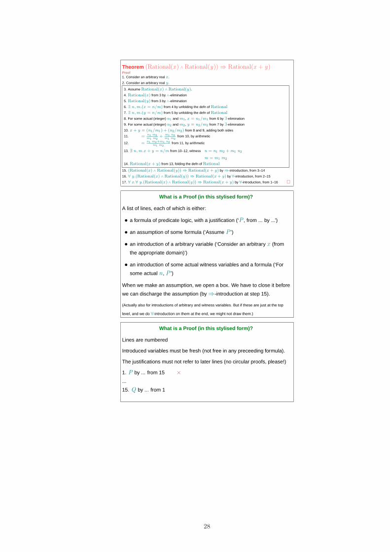
Theorem (Rational(x ) ∧ Rational(y))⇒ Rational(x + y)Proof1. Consider an arbitrary real x .
2. Consider an arbitrary real y .
3. Assume Rational(x) ∧ Rational(y).
4. Rational(x) from 3 by ∧-elimination
5. Rational(y) from 3 by ∧-elimination
6. ∃ n,m.(x = n/m) from 4 by unfolding the defn of Rational
7. ∃ n,m.(y = n/m) from 5 by unfolding the defn of Rational
8. For some actual (integer) n1 and m1, x = n1/m1 from 6 by ∃-elimination
9. For some actual (integer) n2 and m2, y = n2/m2 from 7 by ∃-elimination
10. x + y = (n1/m1) + (n2/m2) from 8 and 9, adding both sides
11. = n1 m2
m1 m2
+ m1 n2
m1 m2
from 10, by arithmetic
12. = n1 m2+m1 n2
m1 m2
from 11, by arithmetic
13. ∃ n,m.x + y = n/m from 10–12, witness n = n1 m2 + m1 n2
m = m1 m2
14. Rational(x + y) from 13, folding the defn of Rational
15. (Rational(x) ∧ Rational(y)) ⇒ Rational(x + y) by ⇒-introduction, from 3–14
16. ∀ y.(Rational(x) ∧ Rational(y)) ⇒ Rational(x + y) by ∀-introduction, from 2–15
17. ∀ x .∀ y.(Rational(x) ∧ Rational(y)) ⇒ Rational(x + y) by ∀-introduction, from 1–16 �
What is a Proof (in this stylised form)?
A list of lines, each of which is either:
• a formula of predicate logic, with a justification (‘P , from ... by ...’)
• an assumption of some formula (‘Assume P ’)
• an introduction of a arbitrary variable (‘Consider an arbitrary x (from
the appropriate domain)’)
• an introduction of some actual witness variables and a formula (‘For
some actual n , P ’)
When we make an assumption, we open a box. We have to close it before
we can discharge the assumption (by⇒-introduction at step 15).
(Actually also for introductions of arbitrary and witness variables. But if these are just at the top
level, and we do ∀-introduction on them at the end, we might not draw them.)
What is a Proof (in this stylised form)?
Lines are numbered
Introduced variables must be fresh (not free in any preceeding formula).
The justifications must not refer to later lines (no circular proofs, please!)
1. P by ... from 15 ×
...
15. Q by ... from 1
28
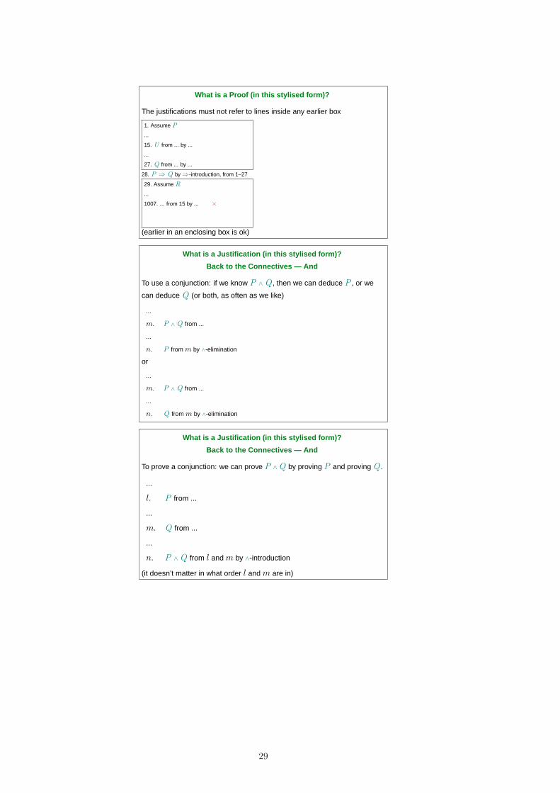
What is a Proof (in this stylised form)?
The justifications must not refer to lines inside any earlier box
1. Assume P
...
15. U from ... by ...
...
27. Q from ... by ...
28. P ⇒ Q by ⇒-introduction, from 1–27
29. Assume R
...
1007. ... from 15 by ... ×
(earlier in an enclosing box is ok)
What is a Justification (in this stylised form)?
Back to the Connectives — And
To use a conjunction: if we know P ∧ Q , then we can deduce P , or we
can deduce Q (or both, as often as we like)
...
m. P ∧ Q from ...
...
n. P from m by ∧-elimination
or
...
m. P ∧ Q from ...
...
n. Q from m by ∧-elimination
What is a Justification (in this stylised form)?
Back to the Connectives — And
To prove a conjunction: we can prove P ∧Q by proving P and proving Q .
...
l. P from ...
...
m. Q from ...
...
n. P ∧ Q from l and m by ∧-introduction
(it doesn’t matter in what order l and m are in)
29
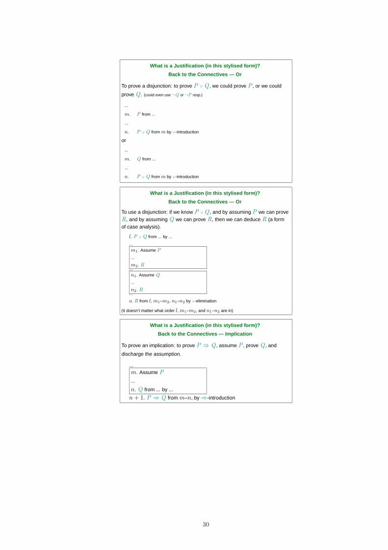
What is a Justification (in this stylised form)?
Back to the Connectives — Or
To prove a disjunction: to prove P ∨ Q , we could prove P , or we could
prove Q . (could even use ¬Q or ¬P resp.)
...
m. P from ...
...
n. P ∨ Q from m by ∨-introduction
or
...
m. Q from ...
...
n. P ∨ Q from m by ∨-introduction
What is a Justification (in this stylised form)?
Back to the Connectives — Or
To use a disjunction: if we know P ∨ Q , and by assuming P we can proveR, and by assuming Q we can prove R, then we can deduce R (a formof case analysis).
l. P ∨ Q from ... by ...
...
m1. Assume P
...
m2. R...
n1. Assume Q
...
n2. R...
o. R from l, m1–m2, n1–n2 by ∨-elimination
(it doesn’t matter what order l, m1–m2, and n1–n2 are in)
What is a Justification (in this stylised form)?
Back to the Connectives — Implication
To prove an implication: to prove P ⇒ Q , assume P , prove Q , and
discharge the assumption.
...m. Assume P
...
n. Q from ... by ...
n + 1. P ⇒ Q from m–n, by⇒-introduction
30
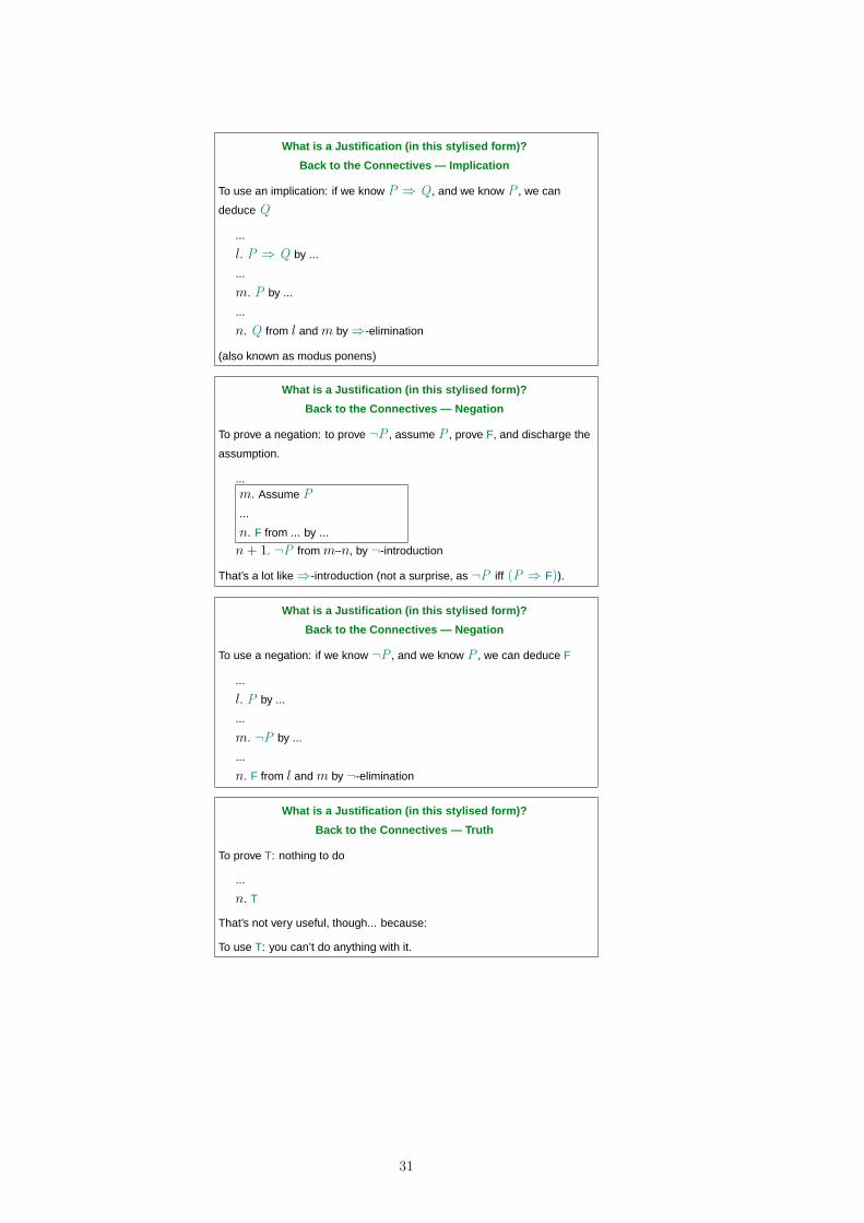
What is a Justification (in this stylised form)?
Back to the Connectives — Implication
To use an implication: if we know P ⇒ Q , and we know P , we can
deduce Q
...
l. P ⇒ Q by ...
...
m. P by ...
...
n. Q from l and m by⇒-elimination
(also known as modus ponens)
What is a Justification (in this stylised form)?
Back to the Connectives — Negation
To prove a negation: to prove ¬P , assume P , prove F, and discharge the
assumption.
...m. Assume P
...
n. F from ... by ...
n + 1. ¬P from m–n, by ¬-introduction
That’s a lot like⇒-introduction (not a surprise, as ¬P iff (P ⇒ F)).
What is a Justification (in this stylised form)?
Back to the Connectives — Negation
To use a negation: if we know ¬P , and we know P , we can deduce F
...
l. P by ...
...
m. ¬P by ...
...
n. F from l and m by ¬-elimination
What is a Justification (in this stylised form)?
Back to the Connectives — Truth
To prove T: nothing to do
...
n. T
That’s not very useful, though... because:
To use T: you can’t do anything with it.
31
What is a Justification (in this stylised form)?
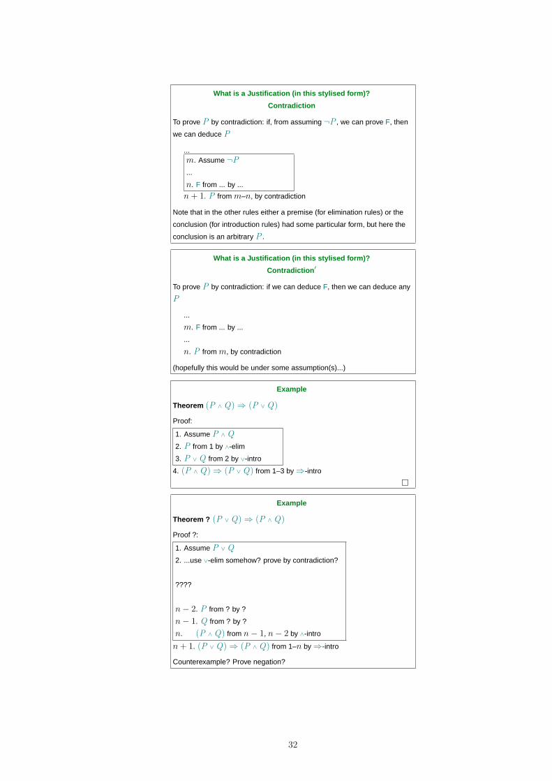
Contradiction
To prove P by contradiction: if, from assuming ¬P , we can prove F, then
we can deduce P
...m. Assume ¬P
...
n. F from ... by ...
n + 1. P from m–n, by contradiction
Note that in the other rules either a premise (for elimination rules) or the
conclusion (for introduction rules) had some particular form, but here the
conclusion is an arbitrary P .
What is a Justification (in this stylised form)?
Contradiction ′
To prove P by contradiction: if we can deduce F, then we can deduce any
P
...
m. F from ... by ...
...
n. P from m, by contradiction
(hopefully this would be under some assumption(s)...)
Example
Theorem (P ∧ Q)⇒ (P ∨ Q)
Proof:
1. Assume P ∧ Q
2. P from 1 by ∧-elim
3. P ∨ Q from 2 by ∨-intro
4. (P ∧ Q)⇒ (P ∨ Q) from 1–3 by⇒-intro
�
Example
Theorem ? (P ∨ Q)⇒ (P ∧ Q)
Proof ?:
1. Assume P ∨ Q
2. ...use ∨-elim somehow? prove by contradiction?
????
n− 2. P from ? by ?
n− 1. Q from ? by ?
n. (P ∧ Q) from n− 1, n− 2 by ∧-intro
n + 1. (P ∨ Q)⇒ (P ∧ Q) from 1–n by⇒-intro
Counterexample? Prove negation?
32
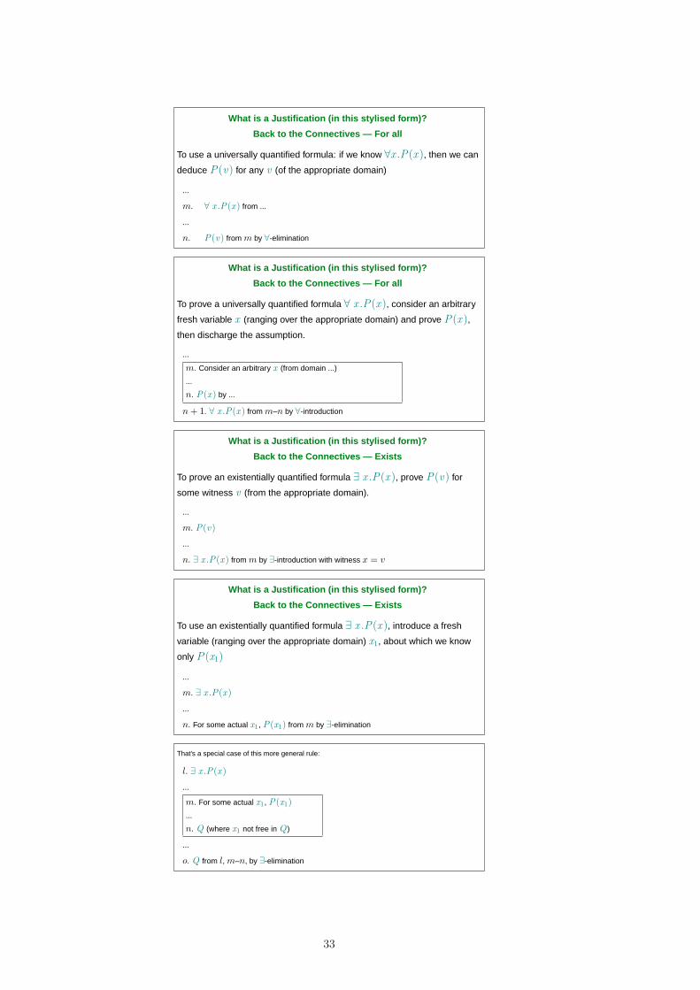
What is a Justification (in this stylised form)?
Back to the Connectives — For all
To use a universally quantified formula: if we know ∀x .P(x ), then we can
deduce P(v) for any v (of the appropriate domain)
...
m. ∀ x .P(x ) from ...
...
n. P(v) from m by ∀-elimination
What is a Justification (in this stylised form)?
Back to the Connectives — For all
To prove a universally quantified formula ∀ x .P(x ), consider an arbitrary
fresh variable x (ranging over the appropriate domain) and prove P(x ),
then discharge the assumption.
...
m. Consider an arbitrary x (from domain ...)
...
n. P(x ) by ...
n + 1. ∀ x .P(x ) from m–n by ∀-introduction
What is a Justification (in this stylised form)?
Back to the Connectives — Exists
To prove an existentially quantified formula ∃ x .P(x ), prove P(v) for
some witness v (from the appropriate domain).
...
m. P(v)
...
n. ∃ x .P(x ) from m by ∃-introduction with witness x = v
What is a Justification (in this stylised form)?
Back to the Connectives — Exists
To use an existentially quantified formula ∃ x .P(x ), introduce a fresh
variable (ranging over the appropriate domain) x1, about which we know
only P(x1)
...
m. ∃ x .P(x )
...
n. For some actual x1, P(x1) from m by ∃-elimination
That’s a special case of this more general rule:
l. ∃ x .P(x )
...
m. For some actual x1, P(x1)
...
n. Q (where x1 not free in Q )
...
o. Q from l, m–n, by ∃-elimination
33
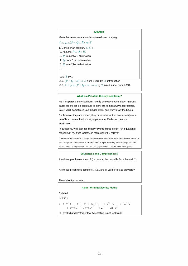
Example
Many theorems have a similar top-level structure, e.g.
∀ x , y , z .(P ∧ Q ∧ R)⇒ S
1. Consider an arbitrary x , y , z .
2. Assume P ∧ Q ∧ R.
3. P from 2 by ∧-elimination
4. Q from 2 by ∧-elimination
5. R from 2 by ∧-elimination
...
215. S by ...
216. (P ∧ Q ∧ R)⇒ S from 2–215 by⇒-introduction
217. ∀ x , y , z .(P ∧ Q ∧ R)⇒ S by ∀-introduction, from 1–216
What is a Proof (in this stylised form)?
NB This particular stylised form is only one way to write down rigorous
paper proofs. It’s a good place to start, but its not always appropriate.
Later, you’ll sometimes take bigger steps, and won’t draw the boxes.
But however they are written, they have to be written down clearly — a
proof is a communication tool, to persuade. Each step needs a
justification.
In questions, we’ll say specifically “by structured proof”, “by equational
reasoning”, “by truth tables”, or, more generally “prove”.
(This is basically the ‘box and line’ proofs from Bornat 2005, which are a linear notation for natural
deduction proofs. More on that in 1B Logic & Proof. If you want to try mechanised proofs, see
jape.org.uk or prover.cs.ru.nl (experiments! — let me know how it goes))
Soundness and Completeness?
Are these proof rules sound? (i.e., are all the provable formulae valid?)
Are these proof rules complete? (i.e., are all valid formulae provable?)
Think about proof search
Aside: Writing Discrete Maths
By hand
In ASCII
P ::= T | F | p | A(x) | P /\ Q | P \/ Q
| P=>Q | P<=>Q | !x.P | ?x.P
In LaTeX (but don’t forget that typesetting is not real work)
34
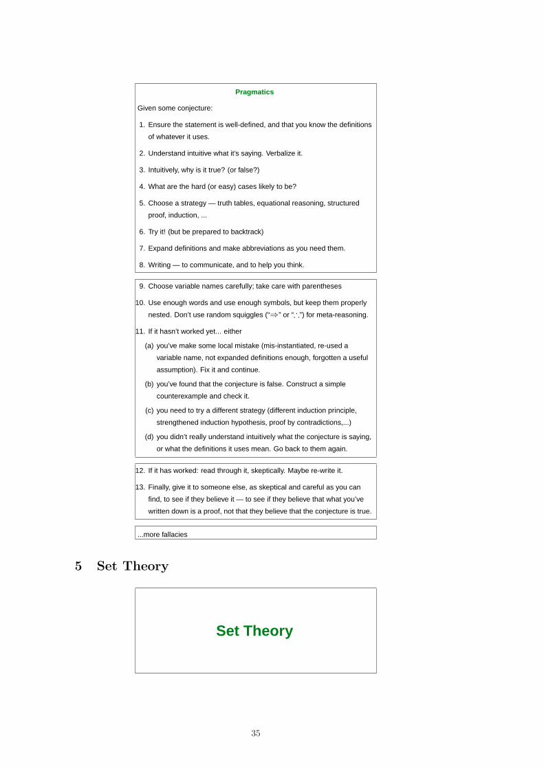
Pragmatics
Given some conjecture:
1. Ensure the statement is well-defined, and that you know the definitions
of whatever it uses.
2. Understand intuitive what it’s saying. Verbalize it.
3. Intuitively, why is it true? (or false?)
4. What are the hard (or easy) cases likely to be?
5. Choose a strategy — truth tables, equational reasoning, structured
proof, induction, ...
6. Try it! (but be prepared to backtrack)
7. Expand definitions and make abbreviations as you need them.
8. Writing — to communicate, and to help you think.
9. Choose variable names carefully; take care with parentheses
10. Use enough words and use enough symbols, but keep them properly
nested. Don’t use random squiggles (“⇒” or “∴”) for meta-reasoning.
11. If it hasn’t worked yet... either
(a) you’ve make some local mistake (mis-instantiated, re-used a
variable name, not expanded definitions enough, forgotten a useful
assumption). Fix it and continue.
(b) you’ve found that the conjecture is false. Construct a simple
counterexample and check it.
(c) you need to try a different strategy (different induction principle,
strengthened induction hypothesis, proof by contradictions,...)
(d) you didn’t really understand intuitively what the conjecture is saying,
or what the definitions it uses mean. Go back to them again.
12. If it has worked: read through it, skeptically. Maybe re-write it.
13. Finally, give it to someone else, as skeptical and careful as you can
find, to see if they believe it — to see if they believe that what you’ve
written down is a proof, not that they believe that the conjecture is true.
...more fallacies
5 Set Theory
Set Theory
35
Set Theory
Now we’ve got some reasoning techniques, but not much to reason about.
Let’s add sets to our language.
What is a set? An unordered collection of elements:
{0, 3, 7} = {3, 0, 7}
might be empty:
{} = ∅ = ∅
might be infinite:
N = {0, 1, 2, 3...}
Z = {...,−1, 0, 1, ...}
R = ...all the real numbers
Some more interesting sets
the set of nodes in a network (encode with N?)
the set of paths between such nodes (encode ??)
the set of polynomial-time computable functions from naturals to naturals
the set of well-typed programs in some programming language
(encode???)
the set of executions of such programs
the set of formulae of predicate logic
the set of valid proofs of such formulae
the set of all students in this room (?)
the set of all sets ×
Basic relationships
membership x ∈ A
3 ∈{1, 3, 5}
2 /∈ {1, 3, 5}
(of course (2 /∈ {1, 3, 5}) iff ¬(2 ∈{3, 5, 1}) )
equality between sets A = B iff ∀ x .x ∈ A⇔ x ∈ B
{1, 2} = {2, 1} = {2, 1, 2, 2} {} 6= {{}}
inclusion or subset A ⊆ B iff ∀ x .x ∈ A⇒ x ∈ B
Properties: ⊆ is reflexive, transitive,
and antisymmetric ((A ⊆ B ∧ B ⊆ A)⇒ A = B)
but not total: {1, 2} 6⊆ {1, 3} 6⊆ {1, 2}
36
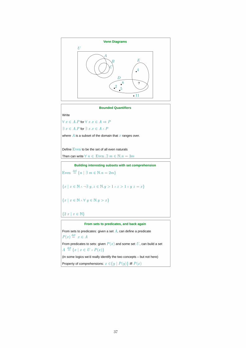
Venn Diagrams
4
B
A
U
C
25
8 ?
11
D
E
Bounded Quantifiers
Write
∀ x ∈ A.P for ∀ x .x ∈ A⇒ P
∃ x ∈ A.P for ∃ x .x ∈ A ∧ P
where A is a subset of the domain that x ranges over.
Define Even to be the set of all even naturals
Then can write ∀ n ∈ Even .∃ m ∈ N.n = 3m
Building interesting subsets with set comprehension
Evendef= {n | ∃ m ∈ N.n = 2m}
{x | x ∈ N ∧ ¬∃ y , z ∈ N.y > 1 ∧ z > 1 ∧ y z = x}
{x | x ∈ N ∧ ∀ y ∈ N.y > x}
{2 x | x ∈ N}
From sets to predicates, and back again
From sets to predicates: given a set A, can define a predicate
P(x )def= x ∈ A
From predicates to sets: given P(x ) and some set U , can build a set
Adef= {x | x ∈ U ∧ P(x )}
(in some logics we’d really identify the two concepts – but not here)
Property of comprehensions: x ∈{y | P(y)} iff P(x )
37
Building new sets from old ones: union, intersection, and di fference
A ∪ Bdef= {x | x ∈ A ∨ x ∈ B}
A ∩ Bdef= {x | x ∈ A ∧ x ∈ B}
A− Bdef= {x | x ∈ A ∧ x /∈ B}
A and B are disjoint iff A ∩ B = {} (symm, not refl or tran)
Building new sets from old ones: union, intersection, and di fference
{1, 2} ∪ {2, 3} = {1, 2, 3}
{1, 2} ∩ {2, 3} = {2}
{1, 2} − {2, 3} = {1}
Properties of union, intersection, and difference
Recall ∨ is associative: P ∨ (Q ∨ R) iff (P ∨ Q) ∨ R
Theorem A ∪ (B ∪ C) = (A ∪ B) ∪ C
Proof
A ∪ (B ∪ C)
1. = {x | x ∈ A ∨ x ∈(B ∪ C)} unfold defn of union
2. = {x | x ∈ A ∨ x ∈{y | y ∈ B ∨ y ∈ C}} unfold defn of union
3. = {x | x ∈ A ∨ (y ∈ B ∨ y ∈ C)} comprehension property
4. = {x | (x ∈ A ∨ y ∈ B) ∨ y ∈ C} by ∨ assoc
5. = (A ∪ B) ∪ C by the comprehension property and folding defn of
union twice �
Some Collected Set Equalities, for Reference
For any sets A, B, and C, all subsets of U
Commutativity:
A ∩ B = B ∩ A (∩-comm)
A ∪ B = B ∪ A (∪-comm)
Associativity:
A ∩ (B ∩ C) = (A ∩ B) ∩ C (∩-assoc)
A ∪ (B ∪ C) = (A ∪ B) ∪ C (∪-assoc)
Distributivity:
A ∩ (B ∪ C) = (A ∩ B)∪ (A ∩ C) (∩-∪-dist)
A ∪ (B ∩ C) = (A ∪ B)∩ (A ∪ C) (∪-∩-dist)
Identity:
A ∩ U = A (∩-id)
A ∪ {} = A (∪-id)
Unit:
A ∩ {} = {} (∩-unit)
A ∪ U = U (∪-unit)
Complement:
A ∩ (U − A) = {} (∩-comp)
A ∪ (U − A) = U (∪-comp)
De Morgan:
U − (A ∩ B) = (U −A)∪ (U −B)
(∩-DM)
U − (A ∪ B) = (U −A)∩ (U −B)
(∪-DM)
38
Example Proof
Theorem {} ⊆ A
Proof
{} ⊆ A
1. iff ∀ x .x ∈{} ⇒ x ∈ A unfolding defn of⊆
2. iff ∀ x .F⇒ x ∈ A use defn of ∈
3. iff ∀ x .T equational reasoning with (F⇒ P) iff T
4. iff T using defn of ∀ �
Another Proof of the Same Theorem
Theorem {} ⊆ A
Another Proof (using the structured rules more explicitly)
1. {} ⊆ A iff ∀ x .x ∈{} ⇒ x ∈ A unfolding defn of⊆
We prove the r.h.s.:
2. Consider an arbitrary x
3. Assume x ∈{}
4. F by defn of ∈
5. x ∈ A from 4, by contradiction
6. x ∈{} ⇒ x ∈ A from 3–5, by⇒-introduction
7. ∀ x .x ∈{} ⇒ x ∈ A from 2–6, by ∀-introduction �
Building new sets from old ones: powerset
Write P(A) for the set of all subsets of a set A.
P{} = {{}}
P{7} = {{}, {7}}
P{1, 2} = {{}, {1}, {2}, {1, 2}}
A ∈ P(A)
(why ‘power’ set?)
Building new sets from old ones: product
Write (a, b) (or sometimes 〈a, b〉) for an ordered pair of a and b
A × Bdef= {(a, b) | a ∈ A ∧ b ∈ B}
Similarly for triples (a, b, c)∈ A × B × C etc.
Pairing is non-commutative: (a, b) 6= (b, a) unless a = b
Pairing is non-associative and distinct from 3-tupling etc:
(a, (b, c)) 6= (a, b, c) 6= ((a, b), c) and
A × (B × C) 6= A × B × C 6= (A × B)× C
Why ‘product’?
{1, 2} × {red, green} = {(1, red), (2, red), (1, green), (2, green)}
39
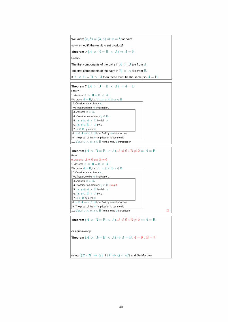
We know (a, b) = (b, a)⇒ a = b for pairs
so why not lift the result to set product?
Theorem ? (A × B = B × A)⇒ A = B
Proof?
The first components of the pairs in A × B are from A.
The first components of the pairs in B × A are from B.
If A × B = B × A then these must be the same, so A = B.
Theorem ? (A × B = B × A)⇒ A = BProof?
1. Assume A × B = B × A
We prove A = B, i.e. ∀ x .x ∈ A⇔ x ∈ B
2. Consider an arbitrary x .
We first prove the⇒ implication.
3. Assume x ∈ A.
4. Consider an arbitrary y ∈ B.
5. (x , y)∈ A × B by defn×
6. (x , y)∈ B × A by 1
7. x ∈ B by defn×
8. x ∈ A⇒ x ∈ B from 3–7 by⇒-introduction
9. The proof of the⇐ implication is symmetric
10. ∀ x .x ∈ A⇔ x ∈ B from 2–9 by ∀-introduction
Theorem (A × B = B × A)∧A 6= ∅ ∧ B 6= ∅ ⇒ A = BProof
0. Assume A 6= ∅ and B 6= ∅
1. Assume A × B = B × A
We prove A = B, i.e. ∀ x .x ∈ A⇔ x ∈ B
2. Consider an arbitrary x .
We first prove the⇒ implication.
3. Assume x ∈ A.
4. Consider an arbitrary y ∈ B using 0
5. (x , y)∈ A × B by defn×
6. (x , y)∈ B × A by 1
7. x ∈ B by defn×
8. x ∈ A⇒ x ∈ B from 3–7 by⇒-introduction
9. The proof of the⇐ implication is symmetric
10. ∀ x .x ∈ A⇔ x ∈ B from 2–9 by ∀-introduction �
Theorem (A × B = B × A)∧A 6= ∅ ∧ B 6= ∅ ⇒ A = B
or equivalently
Theorem (A × B = B × A)⇒ A = B∨A = ∅ ∨ B = ∅
using ((P ∧ R)⇒ Q) iff (P ⇒ Q ∨ ¬R) and De Morgan
40
Aside
Let Adef= {n | n = n + 1}
Is ∀ x ∈ A.x = 7 true?
Or ∀ x ∈ A.x = x + 1? Or ∀ x ∈ A.1 = 2?
Is ∃ x ∈ A.1 + 1 = 2 true?
5.1 Relations, Graphs, and Orders
Relations, Graphs, and Orders
Using Products: Relations
Say a (binary) relation R between two sets A and B is a subset of all
the (a, b) pairs (where a ∈ A and b ∈ B)
R ⊆ A × B (or, or course, R ∈ P(A × B))
Extremes: ∅ and A × B are both relations between A and B
1Adef= {(a, a) | a ∈ A} is the identity relation on A
∅ ⊆ 1A ⊆ A × A
Sometimes write infix: a R bdef= (a, b)∈ R
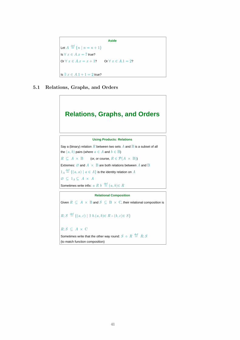
Relational Composition
Given R ⊆ A × B and S ⊆ B × C, their relational composition is
R; Sdef= {(a, c) | ∃ b.(a, b)∈ R ∧ (b, c)∈ S}
R; S ⊆ A × C
Sometimes write that the other way round: S ◦ Rdef= R; S
(to match function composition)
41
Relational Composition
b1
b2
b3
b4
c1
c2
c3
c4
a1
a2
a3
a4
A B C
R; S
b1
b2
b3
b4
c1
c2
c3
c4
a1
a2
a3
a4
A B C
R S
Adef= {a1, a2, a3, a4} B
def= {b1, b2, b3, b4} C
def= {c1, c2, c3, c4}
Rdef= {(a1, b2), (a1, b3), (a2, b3), (a3, b4)}
Sdef= {(b1, c1), (b2, c2), (b3, c2), (b4, c3), (b4, c4)}
R; S = {(a1, c2), (a2, c2), (a3, c3), (a3, c4)}
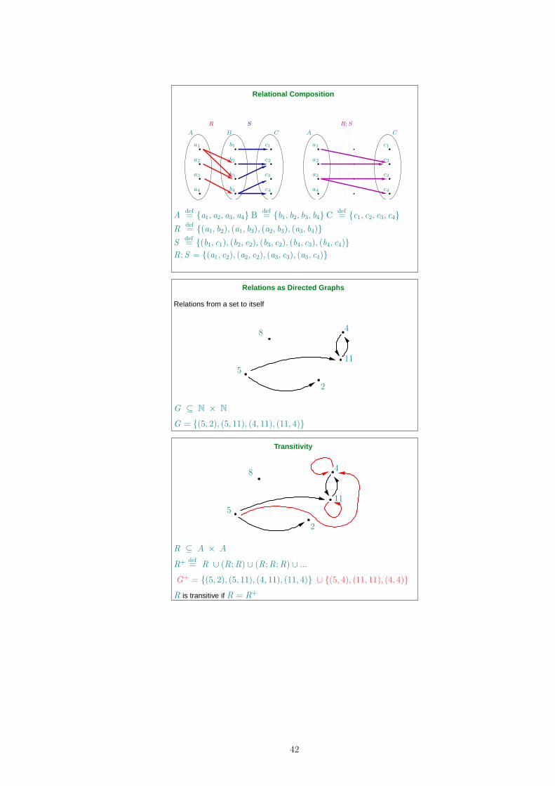
Relations as Directed Graphs
Relations from a set to itself
4
11
8
5
2
G ⊆ N × N
G = {(5, 2), (5, 11), (4, 11), (11, 4)}
Transitivity
4
11
8
5
2
R ⊆ A × A
R+ def= R ∪ (R;R) ∪ (R;R;R) ∪ ...
G+ = {(5, 2), (5, 11), (4, 11), (11, 4)} ∪ {(5, 4), (11, 11), (4, 4)}
R is transitive if R = R+
42
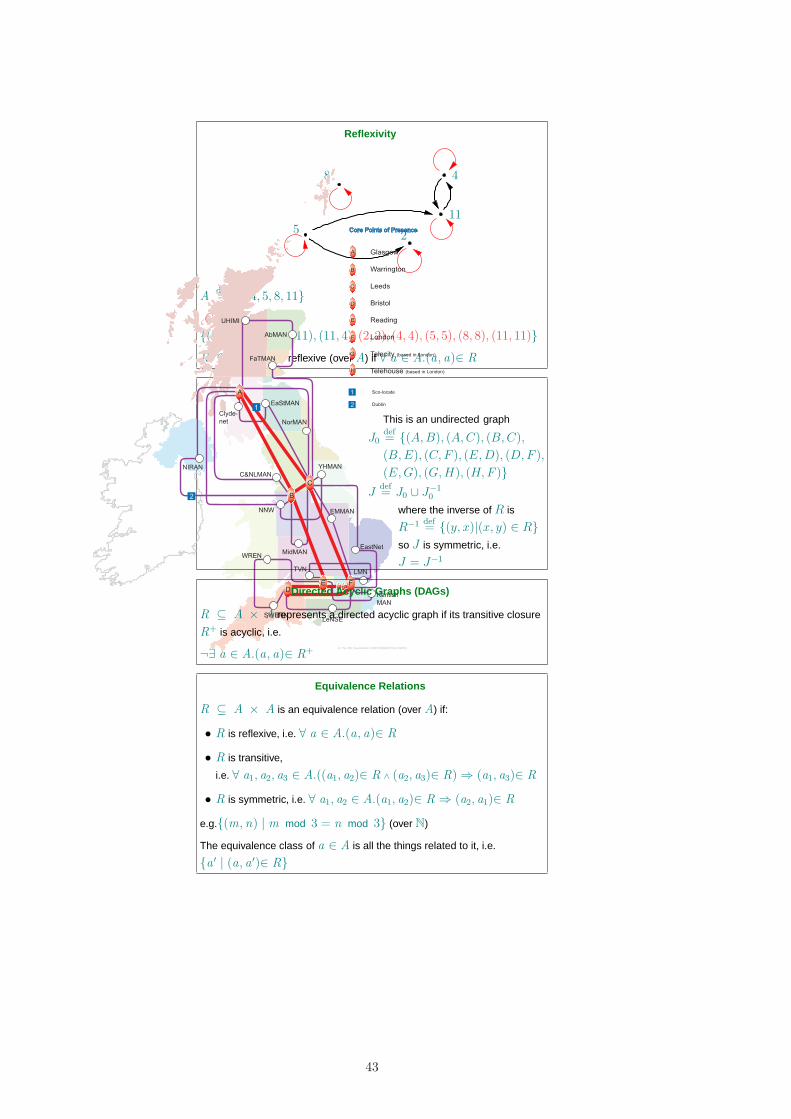
Reflexivity
8
52
4
11
Adef= {2, 4, 5, 8, 11}
G ∪ 1A =
{(5, 2), (5, 11), (4, 11), (11, 4), (2, 2), (4, 4), (5, 5), (8, 8), (11, 11)}
R ⊆ A × A is reflexive (over A) if ∀ a ∈ A.(a, a)∈ R
UHIMI
AbMAN
FaTMAN
Clyde-
net
EaStMAN
NorMAN
NIRANC&NLMAN
YHMAN
NNW EMMAN
MidMANEastNet
WREN
TVN LMN
Kentish
MAN
SWERNLeNSE
1
2
A
B
C
DE F
HG
A
B
C
DE F
HG
© The JNT Association 2006 MS/MAP/004 (09/06)
A
B
C
E
F
G
H
Core Points of Presence
Glasgow
Warrington
Leeds
Bristol
Reading
London
Telecity (based in London)
Telehouse (based in London)
D
1
2
Sco-locate
Dublin
This is an undirected graph
J0def= {(A,B), (A,C), (B,C),
(B,E), (C,F ), (E,D), (D,F ),
(E,G), (G,H), (H,F )}
Jdef= J0 ∪ J−1
0
where the inverse of R is
R−1 def= {(y, x)|(x, y) ∈ R}
so J is symmetric, i.e.
J = J−1
Directed Acyclic Graphs (DAGs)
R ⊆ A × A represents a directed acyclic graph if its transitive closure
R+ is acyclic, i.e.
¬∃ a ∈ A.(a, a)∈ R+
Equivalence Relations
R ⊆ A × A is an equivalence relation (over A) if:
• R is reflexive, i.e. ∀ a ∈ A.(a, a)∈ R
• R is transitive,
i.e. ∀ a1, a2, a3 ∈ A.((a1, a2)∈ R ∧ (a2, a3)∈ R)⇒ (a1, a3)∈ R
• R is symmetric, i.e. ∀ a1, a2 ∈ A.(a1, a2)∈ R ⇒ (a2, a1)∈ R
e.g.{(m, n) | m mod 3 = n mod 3} (over N)
The equivalence class of a ∈ A is all the things related to it, i.e.
{a ′ | (a, a ′)∈ R}
43
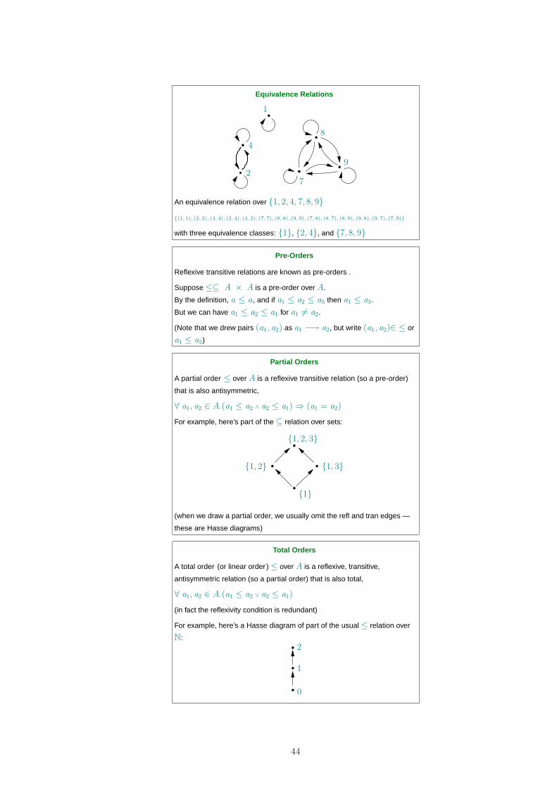
Equivalence Relations
1
2
4
7
9
8
An equivalence relation over {1, 2, 4, 7, 8, 9}
{(1, 1), (2, 2), (4, 4), (2, 4), (4, 2), (7, 7), (8, 8), (9, 9), (7, 8), (8, 7), (8, 9), (9, 8), (9, 7), (7, 9)}
with three equivalence classes: {1}, {2, 4}, and {7, 8, 9}
Pre-Orders
Reflexive transitive relations are known as pre-orders .
Suppose≤⊆ A × A is a pre-order over A.
By the definition, a ≤ a , and if a1 ≤ a2 ≤ a3 then a1 ≤ a3.
But we can have a1 ≤ a2 ≤ a1 for a1 6= a2.
(Note that we drew pairs (a1, a2) as a1 −→ a2, but write (a1, a2)∈ ≤ or
a1 ≤ a2)
Partial Orders
A partial order ≤ over A is a reflexive transitive relation (so a pre-order)
that is also antisymmetric,
∀ a1, a2 ∈ A.(a1 ≤ a2 ∧ a2 ≤ a1)⇒ (a1 = a2)
For example, here’s part of the⊆ relation over sets:
{1}
{1, 3}
{1, 2, 3}
{1, 2}
(when we draw a partial order, we usually omit the refl and tran edges —
these are Hasse diagrams)
Total Orders
A total order (or linear order )≤ over A is a reflexive, transitive,
antisymmetric relation (so a partial order) that is also total,
∀ a1, a2 ∈ A.(a1 ≤ a2 ∨ a2 ≤ a1)
(in fact the reflexivity condition is redundant)
For example, here’s a Hasse diagram of part of the usual≤ relation over
N:
1
2
0
44
Special Relations — Summary
A relation R ⊆ A × A is a directed graph. Properties:
• transitive ∀ a1, a2, a3 ∈ A.(a1 R a2 ∧ a2 R a3)⇒ a1 R a3
• reflexive ∀ a ∈ A.(a R a)
• symmetric ∀ a1, a2 ∈ A.(a1 R a2 ⇒ a2 R a1)
• acyclic ∀ a ∈ A.¬(a R+a)
• antisymmetric ∀ a1, a2 ∈ A.(a1 R a2 ∧ a2 R a1)⇒ a1 = a2
• total ∀ a1, a2 ∈ A.(a1 R a2 ∨ a2 R a1)
Combinations of properties: R is a ...
• directed acyclic graph if the transitive closure is acyclic
• undirected graph if symmetric
• equivalence relation if reflexive, transitive, and symmetric
• pre-order if reflexive and transitive,
• partial order if reflexive, transitive, and antisymmetric
• total order if reflexive, transitive, antisymmetric, and total
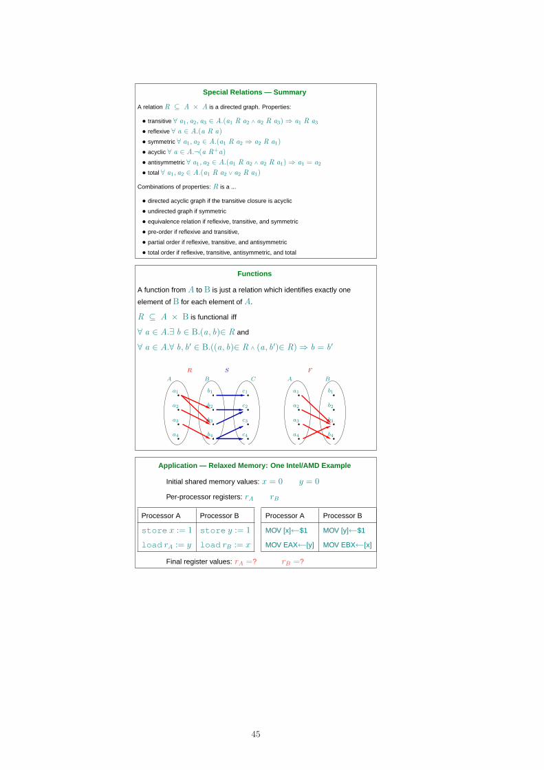
Functions
A function from A to B is just a relation which identifies exactly one
element of B for each element of A.
R ⊆ A × B is functional iff
∀ a ∈ A.∃ b ∈ B.(a, b)∈ R and
∀ a ∈ A.∀ b, b ′ ∈ B.((a, b)∈ R ∧ (a, b ′)∈ R)⇒ b = b ′
b1
b2
b3
b4
c1
c2
c3
c4
a1
a2
a3
a4
A B C
R S
a1
a2
a3
a4
b1
b2
b3
b4
A B
F
Application — Relaxed Memory: One Intel/AMD Example
Initial shared memory values: x = 0 y = 0
Per-processor registers: rA rB
Processor A Processor B
store x := 1 store y := 1
load rA := y load rB := x
Processor A Processor B
MOV [x]←$1 MOV [y]←$1
MOV EAX←[y] MOV EBX←[x]
Final register values: rA =? rB =?
45
Application — Relaxed Memory: One Intel/AMD Example
Initial shared memory values: x = 0 y = 0
Per-processor registers: rA rB
Processor A Processor B
store x := 1 store y := 1
load rA := y load rB := x
Processor A Processor B
MOV [x]←$1 MOV [y]←$1
MOV EAX←[y] MOV EBX←[x]
Final register values: rA =? rB =?
Each processor can do its own store action before the store of the other
processor.
Makes it hard to understand what your programs are doing!
Already a real problem for OS, compiler, and library authors.
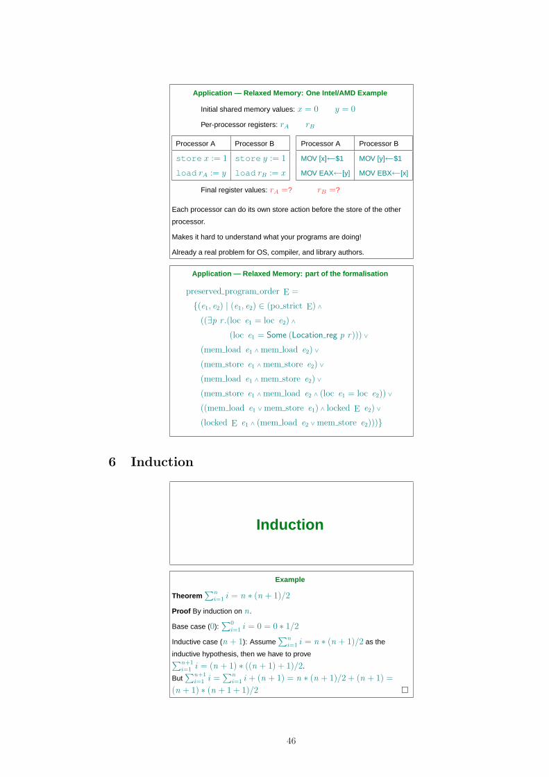
Application — Relaxed Memory: part of the formalisation
preserved program order E =
{(e1, e2) | (e1, e2) ∈ (po strict E) ∧
((∃p r .(loc e1 = loc e2) ∧
(loc e1 = Some (Location reg p r))) ∨
(mem load e1 ∧ mem load e2) ∨
(mem store e1 ∧ mem store e2) ∨
(mem load e1 ∧ mem store e2) ∨
(mem store e1 ∧ mem load e2 ∧ (loc e1 = loc e2)) ∨
((mem load e1 ∨ mem store e1) ∧ locked E e2) ∨
(locked E e1 ∧ (mem load e2 ∨ mem store e2)))}
6 Induction
Induction
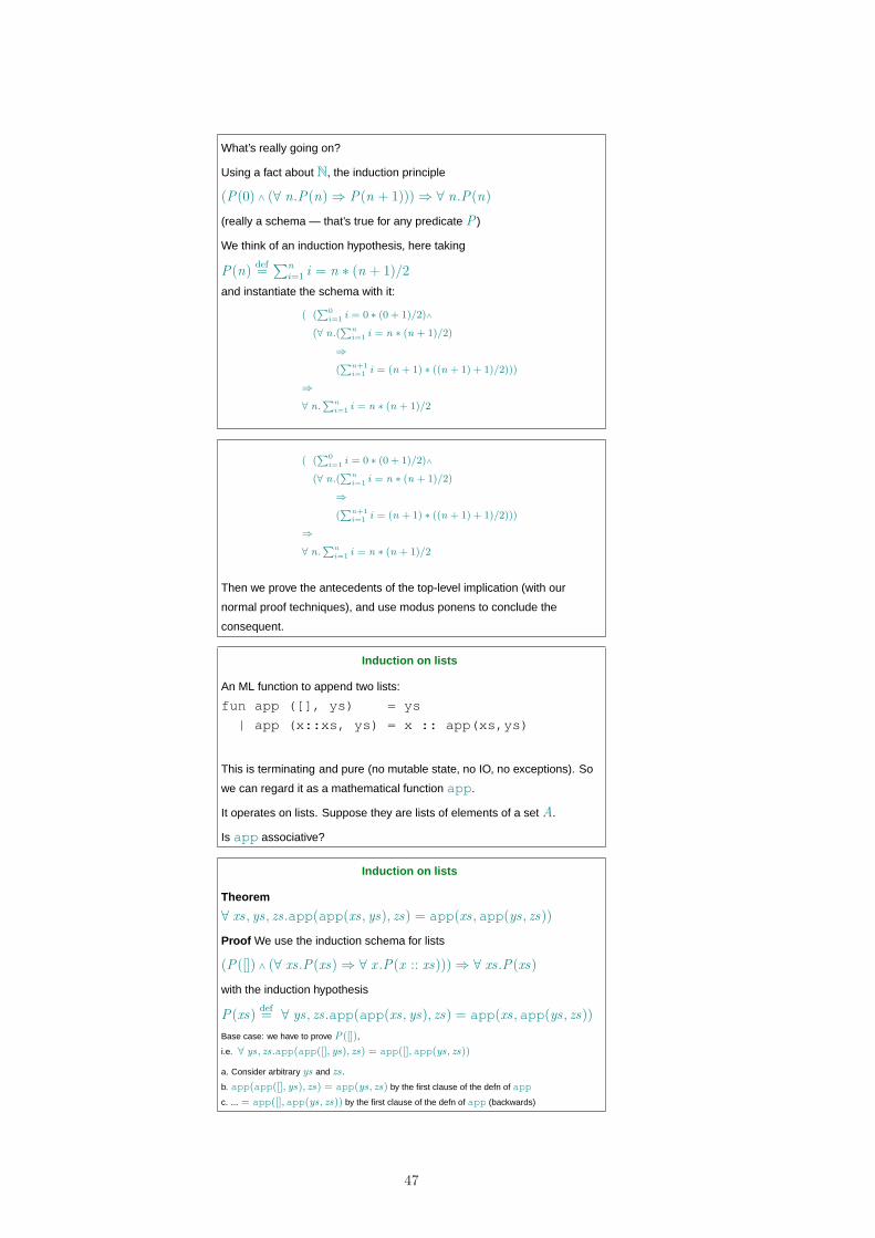
Example
Theorem∑n
i=1 i = n ∗ (n + 1)/2
Proof By induction on n .
Base case (0):∑0
i=1 i = 0 = 0 ∗ 1/2
Inductive case (n + 1): Assume∑n
i=1 i = n ∗ (n + 1)/2 as the
inductive hypothesis, then we have to prove∑n+1
i=1 i = (n + 1) ∗ ((n + 1) + 1)/2.
But∑n+1
i=1 i =∑n
i=1 i + (n + 1) = n ∗ (n + 1)/2 + (n + 1) =
(n + 1) ∗ (n + 1 + 1)/2 �
46
What’s really going on?
Using a fact about N, the induction principle
(P(0) ∧ (∀ n.P(n)⇒ P(n + 1)))⇒ ∀ n.P(n)
(really a schema — that’s true for any predicate P )
We think of an induction hypothesis, here taking
P(n)def=
∑n
i=1 i = n ∗ (n + 1)/2
and instantiate the schema with it:
( (P0
i=1i = 0 ∗ (0 + 1)/2)∧
(∀ n.(P
n
i=1i = n ∗ (n + 1)/2)
⇒
(P
n+1
i=1i = (n + 1) ∗ ((n + 1) + 1)/2)))
⇒
∀ n.P
n
i=1i = n ∗ (n + 1)/2
( (P0
i=1i = 0 ∗ (0 + 1)/2)∧
(∀ n.(P
n
i=1i = n ∗ (n + 1)/2)
⇒
(P
n+1
i=1i = (n + 1) ∗ ((n + 1) + 1)/2)))
⇒
∀ n.P
n
i=1i = n ∗ (n + 1)/2
Then we prove the antecedents of the top-level implication (with our
normal proof techniques), and use modus ponens to conclude the
consequent.
Induction on lists
An ML function to append two lists:
fun app ([], ys) = ys
| app (x::xs, ys) = x :: app(xs,ys)
This is terminating and pure (no mutable state, no IO, no exceptions). So
we can regard it as a mathematical function app.
It operates on lists. Suppose they are lists of elements of a set A.
Is app associative?
Induction on lists
Theorem
∀ xs , ys , zs .app(app(xs , ys), zs) = app(xs ,app(ys , zs))
Proof We use the induction schema for lists
(P([]) ∧ (∀ xs .P(xs)⇒ ∀ x .P(x :: xs)))⇒ ∀ xs .P(xs)
with the induction hypothesis
P(xs)def= ∀ ys , zs .app(app(xs , ys), zs) = app(xs ,app(ys , zs))
Base case: we have to prove P([]),
i.e. ∀ ys, zs.app(app([], ys), zs) = app([],app(ys, zs))
a. Consider arbitrary ys and zs .
b. app(app([], ys), zs) = app(ys, zs) by the first clause of the defn of app
c. ... = app([],app(ys, zs)) by the first clause of the defn of app (backwards)
47
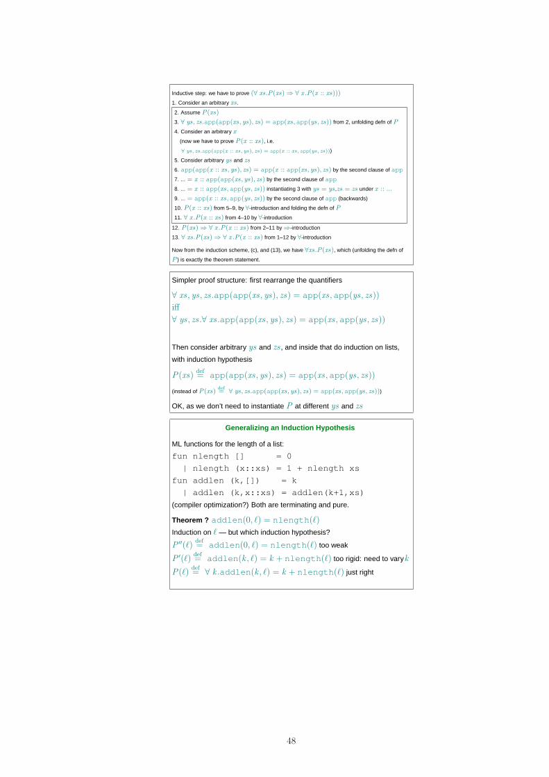
Inductive step: we have to prove (∀ xs.P(xs) ⇒ ∀ x .P(x :: xs)))
1. Consider an arbitrary xs .
2. Assume P(xs)
3. ∀ ys, zs.app(app(xs, ys), zs) = app(xs,app(ys, zs)) from 2, unfolding defn of P
4. Consider an arbitrary x
(now we have to prove P(x :: xs), i.e.
∀ ys, zs.app(app(x :: xs, ys), zs) = app(x :: xs, app(ys, zs)))
5. Consider arbitrary ys and zs
6. app(app(x :: xs, ys), zs) = app(x :: app(xs, ys), zs) by the second clause of app
7. ... = x :: app(app(xs, ys), zs) by the second clause of app
8. ... = x :: app(xs,app(ys, zs)) instantiating 3 with ys = ys ,zs = zs under x :: ...
9. ... = app(x :: xs,app(ys, zs)) by the second clause of app (backwards)
10. P(x :: xs) from 5–9, by ∀-introduction and folding the defn of P
11. ∀ x .P(x :: xs) from 4–10 by ∀-introduction
12. P(xs) ⇒ ∀ x .P(x :: xs) from 2–11 by ⇒-introduction
13. ∀ xs.P(xs) ⇒ ∀ x .P(x :: xs) from 1–12 by ∀-introduction
Now from the induction scheme, (c), and (13), we have ∀xs.P(xs), which (unfolding the defn of
P ) is exactly the theorem statement.
Simpler proof structure: first rearrange the quantifiers
∀ xs , ys , zs .app(app(xs , ys), zs) = app(xs ,app(ys , zs))
iff
∀ ys , zs .∀ xs .app(app(xs , ys), zs) = app(xs ,app(ys , zs))
Then consider arbitrary ys and zs , and inside that do induction on lists,
with induction hypothesis
P(xs)def= app(app(xs , ys), zs) = app(xs ,app(ys , zs))
(instead of P(xs)def= ∀ ys, zs.app(app(xs, ys), zs) = app(xs,app(ys, zs)))
OK, as we don’t need to instantiate P at different ys and zs
Generalizing an Induction Hypothesis
ML functions for the length of a list:
fun nlength [] = 0
| nlength (x::xs) = 1 + nlength xs
fun addlen (k,[]) = k
| addlen (k,x::xs) = addlen(k+1,xs)
(compiler optimization?) Both are terminating and pure.
Theorem ? addlen(0, ℓ) = nlength(ℓ)
Induction on ℓ — but which induction hypothesis?
P ′′(ℓ)def= addlen(0, ℓ) = nlength(ℓ) too weak
P ′(ℓ)def= addlen(k , ℓ) = k + nlength(ℓ) too rigid: need to varyk
P(ℓ)def= ∀ k .addlen(k , ℓ) = k + nlength(ℓ) just right
48
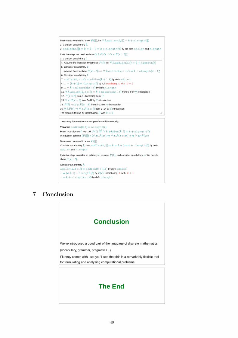
Base case: we need to show P([]), i.e. ∀ k .addlen(k , []) = k + nlength([])
1. Consider an arbitrary k .
2. addlen(k , []) = k = k + 0 = k + nlength(0) by the defn addlen and nlength
Inductive step: we need to show (∀ ℓ.P(ℓ) ⇒ ∀ x .P(x :: ℓ)))
3. Consider an arbitrary ℓ
4. Assume the induction hypothesis P(ℓ), i.e. ∀ k .addlen(k , ℓ) = k + nlength(ℓ)
5. Consider an arbitrary x
(now we have to show P(x :: ℓ), i.e. ∀ k .addlen(k , x :: ℓ) = k + nlength(x :: ℓ))
6. Consider an arbitrary k
7. addlen(k , x :: ℓ) = addlen(k + 1, ℓ) by defn addlen
8. ... = (k + 1) + nlength(ℓ) by 4, instantiating k with k + 1
9. ... = k + nlength(x :: ℓ) by defn nlength
11. ∀ k .addlen(k , x :: ℓ) = k + nlength(x :: ℓ) from 6–9 by ∀-introduction
12. P(x :: ℓ) from 11 by folding defn P
13. ∀ x .P(x :: ℓ) from 5–12 by ∀-introduction
14. P(ℓ) ⇒ ∀ x .P(x :: ℓ) from 4–13 by ⇒-introduction
15. ∀ ℓ.P(ℓ) ⇒ ∀ x .P(x :: ℓ) from 3–14 by ∀-introduction
The theorem follows by instantiating P with k = 0 �
...rewriting that semi-structured proof more idiomatically:
Theorem addlen(0, ℓ) = nlength(ℓ)
Proof Induction on ℓ, with I.H. P(ℓ)def= ∀ k .addlen(k , ℓ) = k + nlength(ℓ)
in induction schema (P([]) ∧ (∀ xs.P(xs) ⇒ ∀ x .P(x :: xs))) ⇒ ∀ xs.P(xs)
Base case: we need to show P([])
Consider an arbitrary k , then addlen(k , []) = k = k + 0 = k + nlength(0) by defn
addlen and nlength
Inductive step: consider an arbitrary ℓ, assume P(ℓ), and consider an arbitrary x . We have to
show P(x :: ℓ).
Consider an arbitrary k .
addlen(k , x :: ℓ) = addlen(k + 1, ℓ) by defn addlen
... = (k + 1) + nlength(ℓ) by P(ℓ), instantiating k with k + 1
... = k + nlength(x :: ℓ) by defn nlength
7 Conclusion
Conclusion
We’ve introduced a good part of the language of discrete mathematics
(vocabulary, grammar, pragmatics...)
Fluency comes with use; you’ll see that this is a remarkably flexible tool
for formulating and analysing computational problems.
The End
49
A Recap: How To Do Proofs
The purpose of this appendix is summarise some of the guidelines about how to provetheorems. This should give you some help in answering questions that begin with “Showthat the following is true . . . ”. It draws on earlier notes by Myra VanInwegen; with manythanks for making the originals available.
The focus here is on doing informal but rigorous proofs. These are rather different from theformal proofs, in Natural Deduction or Sequent Calculus, that will be introduced in the 1BLogic and Proof course. Formal proofs are derivations in one of those proof systems – theyare in a completely well-defined form, but are often far too verbose to deal with by hand(although they can be machine-checked). Informal proofs, on the other hand, are the usualmathematical notion of proof: written arguments to persuade the reader that you could, ifpushed, write a fully formal proof.
This is important for two reasons. Most obviously, you should learn how to do these proofs.More subtly, but more importantly, only by working with the mathematical definitions insome way can you develop a good intuition for what they mean — trying to do some proofsis the best way of understanding the definitions.
A.1 How to go about it
Proofs differ, but for many of those you meet the following steps should be helpful.
1. Make sure the statement of the conjecture is precisely defined. In particular, makesure you understand any strange notation, and find the definitions of all the auxiliarygadgets involved (e.g. definitions of any typing or reduction relations mentioned in thestatement, or any other predicates or functions).
2. Try to understand at an intuitive level what the conjecture is saying – verbalize outloud the basic point. For example, for a Type Preservation conjecture, the basicpoint might be something like “if a well-typed configuration reduces, the result is stillwell-typed (with the same type)”.
3. Try to understand intuitively why it is true (or false...). Identify what the mostinteresting cases might be — the cases that you think are most likely to be suspicious,or hard to prove. Sometimes it’s good to start with the easy cases (if the settingis unfamiliar to you); sometimes it’s good to start with the hard cases (to find anyinteresting problems as soon as possible).
4. Think of a good basic strategy. This might be:
(a) simple logic manipulations;
(b) collecting together earlier results, again by simple logic; or
(c) some kind of induction.
5. Try it! (remembering you might have to backtrack if you discover you picked a strategythat doesn’t work well for this conjecture). This might involve any of the following:
(a) Expanding definitions, inlining them. Sometimes you can just blindly expand alldefinitions, but more often it’s important to expand only the definitions whichyou want to work with the internal structure of — otherwise things just get tooverbose.
(b) Making abbreviations — defining a new variable to stand for some complex gadgetyou’re working with, saying e.g.
where e = (let x:int = 7+2 in x+x)
Take care with choosing variable names.
50
(c) Doing equational reasoning, e.g.
e = e1 by ...
= e2 by ...
= e3 as ...
Here the e might be any mathematical object — arithmetic expressions, or ex-pressions of some grammar, or formulae. Some handy equations over formulaeare given in §A.2.2.
(d) Proving a formula based on its structure. For example, to prove a formula ∀x ∈S.P (x) you would often assume you have an arbitrary x and then try to proveP (x).
Take an arbitrary x ∈ S.We now have to show P (x):
This is covered in detail in §A.2.3. Much proof is of this form, automaticallydriven by the structure of the formula.
(e) Using an assumption you’ve made above.
(f) Induction. As covered in the 1B Semantics notes, there are various kinds of induc-tion you might want to use: mathematical induction over the natural numbers,structural induction over the elements of some grammar, or rule induction overthe rules defining some relation (especially a reduction or typing relation). Foreach, you should:
i. Decide (and state!) what kind of induction you’re using. This may needsome thought and experience, and you might have to backtrack.
ii. Remind yourself what the induction principle is exactly.
iii. Decide on the induction hypothesis you’re going to use, writing down a pred-icate Φ which is such that the conclusion of the induction principle impliesthe thing you’re trying to prove. Again, this might need some thought. Takecare with the quantifiers here — it’s suspicious if your definition of Φ hasany globally-free variables...
iv. Go through each of the premises of the induction principle and prove each one(using any of these techniques as appropriate). Many of those premises willbe implications, e.g. ∀x ∈ N.Φ(x)⇒ Φ(x + 1), for which you can do a proofbased on the structure of the formula — taking an arbitrary x, assumingΦ(x), and trying to prove Φ(x+1). Usually at some point in the latter you’dmake use of the assumption Φ(x).
6. In all of the above, remember: the point of doing a proof on paper is to use theformalism to help you think — to help you cover all cases, precisely — and also tocommunicate with the reader. For both, you need to write clearly:
(a) Use enough words! “Assume”, “We have to show”, “By such-and-such we know”,“Hence”,...
(b) Don’t use random squiggles. It’s good to have formulae properly nested withintext, with and no “⇒” or “∴” between lines of text.
7. If it hasn’t worked yet... either
(a) you’ve make some local mistake, e.g. mis-instantiated something, or used thesame variable for two different things, or not noticed that you have a definitionyou should have expanded or an assumption you should have used. Fix it andcontinue.
51
(b) you’ve discovered that the conjecture is really false. Usually at this point it’sa good idea to construct a counterexample that is as simple as possible, and tocheck carefully that it really is a counterexample.
(c) you need to try a different strategy — often, to use a different induction principleor to strengthen your induction hypothesis.
(d) you didn’t really understand intuitively what the conjecture is saying, or whatthe definitions it uses mean. Go back to them again.
8. If it has worked: read through it, skeptically, and check. Maybe you’ll need to re-writeit to make it comprehensible: proof discovery is not the same as proof exposition. Seethe example proofs in the Semantics notes.
9. Finally, give it to someone else, as skeptical and careful as you can find, to see if theybelieve it — to see if they believe that what you’ve written down is a proof, not thatthey believe that the conjecture is true.
52
A.2 And in More Detail...
In the following, I’ll call any logic statement a formula. In general, what we’ll be trying todo is prove a formula, using a collection of formulas that we know to be true or are assumingto be true. There’s a big difference between using a formula and proving a formula. In fact,what you do is in many ways opposite. So, I’ll start by explaining how to prove a formula.
A.2.1 Meet the Connectives
Here are the logical connectives and a very brief decription of what each means.
P ∧Q P and Q are both trueP ∨Q P is true, or Q is true, or both are true¬P P is not true (P is false)
P ⇒ Q if P is true then Q is trueP ⇔ Q P is true exactly when Q is true
∀x ∈ S.P (x) for all x in S, P is true of x∃x ∈ S.P (x) there exists an x in S such that P holds of x
A.2.2 Equivalences
These are formulas that mean the same thing, and this is indicated by a iff between them.The fact that they are equivalent to each other is justified by the truth tables of the con-nectives.
definition of ⇒ P ⇒ Q iff ¬P ∨Qdefinition of ⇔ P ⇔ Q iff (P ⇒ Q) ∧ (Q⇒ P )definition of ¬ ¬P iff P ⇒ false
de Morgan’s Laws ¬(P ∧Q) iff ¬P ∨ ¬Q¬(P ∨Q) iff ¬P ∧ ¬Q
extension to quantifiers ¬(∀x.P (x)) iff ∃x.¬P (x)¬(∃x.P (x)) iff ∀x.¬P (x)
distributive laws P ∨ (Q ∧R) iff (P ∨Q) ∧ (P ∨R)P ∧ (Q ∨R) iff (P ∧Q) ∨ (P ∧R)
coalescing quantifiers (∀x.P (x)) ∧ (∀x.Q(x)) iff ∀x.(P (x) ∧Q(x))(∃x.P (x)) ∨ (∃x.Q(x)) iff ∃x.(P (x) ∨Q(x))
these ones apply if (∀x.P (x)) ∧Q iff (∀x.P (x) ∧Q)x is not free in Q (∀x.P (x)) ∨Q iff (∀x.P (x) ∨Q)
(∃x.P (x)) ∧Q iff (∃x.P (x) ∧Q)(∃x.P (x)) ∨Q iff (∃x.P (x) ∨Q)
A.2.3 How to Prove a Formula
For each of the logical connectives, I’ll explain how to handle them.
∀x ∈ S.P (x) This means “For all x in S, P is true of x.” Such a formula is called a
universally quantified formula. The goal is to prove that the property P , which has somexs somewhere in it, is true no matter what value in S x takes on. Often the “∈ S” is leftout. For example, in a discussion of lists, you might be asked to prove ∀l.length l > 0 ⇒∃x. member(x, l). Obviously, l is a list, even if it isn’t explicitly stated as such.
There are several choices as to how to prove a formula beginning with ∀x. The standardthing to do is to just prove P (x), not assuming anything about x. Thus, in doing the proofyou sort of just mentally strip off the ∀x. What you would write when doing this is “Let x beany S”. However, there are some subtleties—if you’re already using an x for something else,
53
you can’t use the same x, because then you would be assuming something about x, namelythat it equals the x you’re already using. In this case, you need to use alpha-conversion1 tochange the formula you want to prove to ∀y ∈ S.P (y), where y is some variable you’re notalready using, and then prove P (y). What you could write in this case is “Since x is alreadyin use, we’ll prove the property of y”.
An alternative is induction, if S is a set that is defined with a structural definition. Manyobjects you’re likely to be proving properties of are defined with a structural definition.This includes natural numbers, lists, trees, and terms of a computer language. Sometimesyou can use induction over the natural numbers to prove things about other objects, suchas graphs, by inducting over the number of nodes (or edges) in a graph.
You use induction when you see that during the course of the proof you would need to usethe property P for the subparts of x in order to prove it for x. This usually ends up beingthe case if P involves functions defined recursively (i.e., the return value for the functiondepends on the function value on the subparts of the argument).
A special case of induction is case analysis. It’s basically induction where you don’t use theinductive hypothesis: you just prove the property for each possible form that x could have.Case analysis can be used to prove the theorem about lists above.
A final possibility (which you can use for all formulas, not just for universally quantifiedones) is to assume the contrary, and then derive a contradiction.
∃x ∈ S.P (x) This says “There exists an x in S such that P holds of x.” Such a formula is
called an existentially quantified formula. The main way to prove this is to figure out whatx has to be (that is, to find a concrete representation of it), and then prove that P holds ofthat value. Sometimes you can’t give a completely specified value, since the value you pickfor x has to depend on the values of other things you have floating around. For example,say you want to prove
∀x, y ∈ ℜ.x < y ∧ sin x < 0 ∧ sin y > 0⇒ ∃z.x < z ∧ z < y ∧ sin z = 0
where ℜ is the set of real numbers. By the time you get to dealing with the ∃z.x < z ∧ z <y ∧ sin z = 0, you will have already assumed that x and y were any real numbers. Thus thevalue you choose for z has to depend on whatever x and y are.
An alternative way to prove ∃x ∈ S.P (x) is, of course, to assume that no such x exists, andderive a contradiction.
To summarize what I’ve gone over so far: to prove a universally quantified formula, you mustprove it for a generic variable, one that you haven’t used before. To prove an existentiallyquantified formula, you get to choose a value that you want to prove the property of.
P ⇒ Q This says “If P is true, then Q is true”. Such a formula is called an implication,
and it is often pronounced “P implies Q”. The part before the ⇒ sign (here P ) is calledthe antecedent, and the part after the ⇒ sign (here Q) is called the consequent. P ⇒ Q isequivalent to ¬P ∨Q, and so if P is false, or if Q is true, then P ⇒ Q is true.
The standard way to prove this is to assume P , then use it to help you prove Q. Note thatI said that you will be using P . Thus you will need to follow the rules in Section A.2.4 todeal with the logical connectives in P .
Other ways to prove P ⇒ Q involve the fact that it is equivalent to ¬P ∨Q. Thus, you canprove ¬P without bothering with Q, or you can just prove Q without bothering with P .To reason by contradiction you assume that P is true and that Q is not true, and derive acontradiction.
1Alpha-equivalence says that the name of a bound variable doesn’t matter, so you can change it at will(this is called alpha-conversion). You’ll get to know the exact meaning of this soon enough so I won’t explainthis here.
54
Another alternative is to prove the contrapositive: ¬Q⇒ ¬P , which is equivalent to it.
P ⇔ Q This says “P is true if and only if Q is true”. The phrase “if and only if” is usually
abbreviated “iff”. Basically, this means that P and Q are either both true, or both false.
Iff is usually used in two main ways: one is where the equivalence is due to one formulabeing a definition of another. For example, A ⊆ B ⇔ (∀x. x ∈ A⇒ x ∈ B) is the standarddefinition of subset. For these iff statements, you don’t have to prove them. The other useof iff is to state the equivalence of two different things. For example, you could define anSML function fact:
fun fact 0 = 1
| fact n = n * fact (n - 1)
Since in SML whole numbers are integers (both positive and negative) you may be askedto prove: fact x terminates ⇔ x ≥ 0. The standard way to do this is us the equivalenceP ⇔ Q is equivalent to P ⇒ Q ∧ Q ⇒ P . And so you’d prove that (fact x terminates ⇒x ≥ 0) ∧ (x ≥ 0⇒ fact x terminates).
¬P This says “P is not true”. It is equivalent to P ⇒ false, thus this is one of the waysyou prove it: you assume that P is true, and derive a contradiction (that is, you provefalse). Here’s an example of this, which you’ll run into later this year: the undecidabilityof the halting problem can be rephrased as ¬∃x ∈ RM. x solves the halting problem, whereRM is the set of register machines. The proof of this in your Computation Theory notesfollows exactly the pattern I described—it assumes there is such a machine and derives acontradiction.
The other major way to prove ¬P is to figure out what the negation of P is, using equiva-lences like De Morgan’s Law, and then prove that. For example, to prove ¬∀x ∈ N . ∃y ∈N . x = y2, where N is the set of natural numbers, you could push in the negation to get:∃x ∈ N . ∀y ∈ N . x 6= y2, and then you could prove that.
P ∧Q This says “P is true and Q is true”. Such a formula is called a conjunction. To
prove this, you have to prove P , and you have to prove Q.
P ∨Q This says “P is true or Q is true”. This is inclusive or: if P and Q are both true,
then P ∨Q is still true. Such a formula is called a disjunction. To prove this, you can proveP or you can prove Q. You have to choose which one to prove. For example, if you need toprove (5 mod 2 = 0) ∨ (5 mod 2 = 1), then you’ll choose the second one and prove that.
However, as with existentials, the choice of which one to prove will often depend on thevalues of other things, like universally quantified variables. For example, when you arestudying the theory of programming languages (you will get a bit of this in Semantics), youmight be asked to prove
∀P ∈ ML. P is properly typed⇒(the evaluation of P runs forever) ∨ (P evaluates to a value)
where ML is the set of all ML programs. You don’t know in advance which of these will bethe case, since some programs do run forever, and some do evaluate to a value. Generally,the best way to prove the disjunction in this case (when you don’t know in advance whichwill hold) is to use the equivalence with implication. For example, you can use the factthat P ∨ Q is equivalent to ¬P ⇒ Q, then assume ¬P , then use this to prove Q. Forexample, your best bet to proving this programming languages theorem is to assume thatthe evaluation of P doesn’t run forever, and use this to prove that P evaluates to a value.
55
A.2.4 How to Use a Formula
You often end up using a formula to prove other formulas. You can use a formula if someonehas already proved that it’s true, or you are assuming it because it was in an implication,namely, the A in A⇒ B. For each logical connective, I’ll tell you how to use it.
∀x ∈ S.P (x) This formula says that something is true of all elements of S. Thus, when
you use it, you can pick any value at all to use instead of x (call it v), and then you can useP (v).
∃x ∈ S.P (x) This formula says that there is some x that satisfies P . However, you do not
know what it is, so you can not assume anything about it. The usual approach it to justsay that the thing that is being said to exist is just x, and use the fact that P holds of x toprove something else. However, if you’re already using an x for something else, you have topick another variable to represent the thing that exists.
To summarize this: to use a universally quantified formula, you can choose any value, anduse that the formula holds for that variable. To use an existentially quantified formula, youmust not assume anything about the value that is said to exists, so you just use a variable(one that you haven’t used before) to represent it. Note that this is more or less oppositeof what you do when you prove a universally or existentially quantified formula.
¬P Usually, the main use of this formula is to prove the negation of something else.An example is the use of reduction to prove the unsolvability of various problems in theComputation Theory (you’ll learn all about this in 1B). You want to prove ¬Q, where Qstates that a certain problem (Problem 1) is decidable (in other words, you want to provethat Problem 1 is not decidable). You know ¬P , where P states that another problem(Problem 2) is decidable (i.e. ¬P says that Problem 2 is not decidable). What you dobasically is this. You first prove Q⇒ P , which says that if Problem 1 is decidable, then sois Problem 2. Since Q ⇒ P iff ¬P ⇒ ¬Q, you have now proved ¬P ⇒ ¬Q. You alreadyknow ¬P , so you use modus ponens2 to get that ¬Q.
P ⇒ Q The main way to use this is that you prove P , and then you use modus ponens to
get Q, which you can then use.
P ⇔ Q The main use of this is to replace an occurrence of P in a formula with Q, and
vise versa.
P ∧Q Here you can use both P and Q. Note, you’re not required to use both of them, but
they are both true and are waiting to be used by you if you need them.
P ∨Q Here, you know that one of P or Q is true, but you do not know which one. To use
this to prove something else, you have to do a split: first you prove the thing using P , thenyou prove it using Q.
Note that in each of the above, there is again a difference in the way you use a formula,verses the way you prove it. They are in a way almost opposites. For example, in provingP ∧ Q, you have to prove both P and Q, but when you are using the formula, you don’thave to use both of them.
A.3 An Example
Here, we’ll look forward to Regular Languages and Finite Automata (this might not makemuch sense until you get to that). The Pumping Lemma for regular sets (PL for short) is
2Modus ponens says that if A ⇒ B and A are both true, then B is true.
56
an astonishingly good example of the use of quantifiers. We’ll go over the proof and use ofthe PL, paying special attention to the logic of what’s happening.
A.3.1 Proving the PL
My favorite book on regular languages, finite automata, and their friends is the Hopcroftand Ullman book Introduction to Automata Theory, Languages, and Computation. Youshould locate this book in your college library, and if it isn’t there, insist that your DoSorder it for you.
In the Automata Theory book, the Pumping Lemma is stated as: “Let L be a regular set.Then there is a constant n such that if z is any word in L, and |z| ≥ n, we may write z = uvwin such a way that |uv| ≤ n, |v| ≥ 1, and for all i ≥ 0, uviw is in L.” The Pumping Lemmais, in my experience, one of the most difficult things about learning automata theory. Itis difficult because people don’t know what to do with all those logical connectives. Let’swrite it as a logical formula.
∀L ∈ RegularLanguages.∃n. ∀z ∈ L. |z| ≥ n⇒∃u v w. z = uvw ∧ |uv| ≤ n ∧ |v| ≥ 1 ∧∀i ≥ 0. uviw ∈ L
Complicated, eh? Well, let’s prove it, using the facts that Hopcroft and Ullman haveestablished in the chapters previous to the one wih the PL. I’ll give the proof and put insquare brackets comments about what I’m doing.
Let L be any regular language. [Here I’m dealing with the ∀L ∈ RegularLanguages bystating that I’m not assuming anything about L.] Let M be a minimal-state deterministicfinite state machine accepting L. [Here I’m using a fact that Hopcroft and Ullman havealready proved about the equivalence of regular languages and finite automata.] Let n bethe number of states in this finite state machine. [I’m dealing with the ∃n by giving a veryspecific value of what it will be, based on the arbitrary L.] Let z be any word in L. [ThusI deal with ∀z ∈ L.] Assume that |z| ≥ n. [Thus I’m taking care of the ⇒ by assuming theantecedent.]
Say z is written a1a2 . . . am, where m ≥ n. Consider the states that M is in during theprocessing of the first n symbols of z, a1a2 . . . an. There are n + 1 of these states. Sincethere are only n states in M , there must be a duplicate. Say that after symbols aj and ak
we are in the same state, state s (i.e. there’s a loop from this state that the machine goesthrough as it accepts z), and say that j < k. Now, let u = a1a2 . . . aj . This represents thepart of the string that gets you to state s the first time. Let v = aj+1 . . . ak. This representsthe loop that takes you from s and back to it again. Let w = ak+1 . . . am, the rest of wordz. [We have chosen definite values for u, v, and w.] Then clearly z = uvw, since u, v, andw are just different sections of z. |uv| ≤ n since u and v occur within the first n symbolsof z. |v| ≥ 1 since j < k. [Note that we’re dealing with the formulas connected with ∧ byproving each of them.]
Now, let i be a natural number (i.e. ≥ 0). [This deals with ∀i ≥ 0.] Then uviw ∈ L. [Finallyour conclusion, but we have to explain why this is true.] This is because we can repeat theloop from s to s (represented by v) as many times as we like, and the resulting word willstill be accepted by M .
A.3.2 Using the PL
Now we use the PL to prove that a language is not regular. This is a rewording of Example3.1 from Hopcroft and Ullman. I’ll show that L = {0i2 |i is an integer, i ≥ 1} is not regular.Note that L consists of all strings of 0’s whose length is a perfect square. I will use the PL.I want to prove that L is not regular. I’ll assume the negation (i.e., that L is regular) and
57
derive a contradiction. So here we go. Remember that what I’m emphasizing here is notthe finite automata stuff itself, but how to use a complicated theorem to prove somethingelse.
Assume L is regular. We will use the PL to get a contradiction. Since L is regular, the PLapplies to it. [We note that we’re using the ∀ part of the PL for this particular L.] Let nbe as described in the PL. [This takes care of using the ∃n. Note that we are not assuming
anything about its actual value, just that it’s a natural number.] Let z = 0n2
. [Since the PLsays that something is true of all zs, we can choose the one we want to use it for.] So by thePL there exist u, v, and w such that z = uvw, |uv| ≤ n, |v| ≥ 1. [Note that we don’t assumeanything about what the u, v, and w actually are; the only thing we know about them iswhat the PL tells us about them. This is where people trying to use the PL usually screwup.] The PL then says that for any i, then uviw ∈ L. Well, then uv2w ∈ L. [This is usingthe ∀i ≥ 0 bit.] However, n2 < |uv2w| ≤ n2 + n, since 1 ≤ |v| ≤ n. But n2 + n < (n + 1)2.Thus |uv2w| lies properly between n2 and (n + 1)2 and is thus not a perfect square. Thusuv2w is not in L. This is a contradiction. Thus our assumption (that L was regular) wasincorrect. Thus L is not a regular language.
58
B Exercises
Exercise Sheet 1: Propositional Logic
1. Let p stand for the proposition“I bought a lottery ticket”and q for“I won the jackpot”.Express the following as natural English sentences:
(a) ¬p
(b) p ∨ q
(c) p ∧ q
(d) p ⇒ q
(e) ¬p ⇒ ¬q
(f) ¬p ∨ (p ∧ q)
2. Formalise the following in terms of atomic propositions R, B, and W , first makingclear how they correspond to the English text.
(a) Berries are ripe along the path, but rabbits have not been seen in the area.
(b) Rabbits have not been seen in the area, and walking on the path is safe, butberries are ripe along the path.
(c) If berries are ripe along the path, then walking is safe if and only if rabbits havenot been seen in the area.
(d) It is not safe to walk along the path, but rabbits have not been seen in the areaand the berries along the path are ripe.
(e) For walking on the path to be safe, it is necessary but not sufficient that berriesnot be ripe along the path and for rabbits not to have been seen in the area.
(f) Walking is not safe on the path whenever rabbits have been seen in the area andberries are ripe along the path.
3. Formalise these statements and determine (with truth tables or otherwise) whetherthey are consistent (i.e. if there are some assumptions on the atomic propositions thatmake it true): “The system is in a multiuser state if and only if it is operating normally.If the system is operating normally, the kernel is functioning. Either the kernel is notfunctioning or the system is in interrupt mode. If the system is not in multiuser state,then it is in interrupt mode. The system is not in interrupt mode.”
4. When is a propositional formula P valid? When is P satisfiable?
5. For each of the following propositions, construct a truth table and state whether theproposition is valid or satisfiable. (For brevity, you can just write one truth table withmany columns.)
(a) p ∧ ¬p
(b) p ∨ ¬p
(c) (p ∨ ¬q)⇒ q
(d) (p ∨ q)⇒ (p ∧ q)
(e) (p ⇒ q)⇔ (¬q ⇒ ¬p)
(f) (p ⇒ q)⇒ (q ⇒ p)
6. For each of the following propositions, construct a truth table and state whether theproposition is valid or satisfiable.
59
(a) p ⇒ (¬q ∨ r)
(b) ¬p ⇒ (q ⇒ r)
(c) (p ⇒ q) ∨ (¬p ⇒ r)
(d) (p ⇒ q) ∧ (¬p ⇒ r)
(e) (p ⇔ q) ∨ (¬q ⇔ r)
(f) (¬p ⇔ ¬q)⇔ (q ⇔ r)
7. Formalise the following and, by writing truth tables for the premises and conclusion,determine whether the arguments are valid.
(a)Either John isn’t stupid and he is lazy, or he’s stupid.John is stupid.Therefore, John isn’t lazy.
(b)The butler and the cook are not both innocentEither the butler is lying or the cook is innocentTherefore, the butler is either lying or guilty
8. Use truth tables to determine which of the following are equivalent to each other:
(a) P
(b) ¬P
(c) P ⇒ F
(d) P ⇒ T
(e) F⇒ P
(f) T⇒ P
(g) ¬¬P
9. Use truth tables to determine which of the following are equivalent to each other:
(a) (P ∧ Q) ∨ (¬P ∧ ¬Q)
(b) ¬P ∨ Q
(c) (P ∨ ¬Q) ∧ (Q ∨ ¬P)
(d) ¬(P ∨ Q)
(e) (Q ∧ P) ∨ ¬P
10. Imagine that a logician puts four cards on the table in front of you. Each card has anumber on one side and a letter on the other. On the uppermost faces, you can seeE, K, 4, and 7. He claims that if a card has a vowel on one side, then it has an evennumber on the other. How many cards do you have to turn over to check this?
11. Give a truth-table definition of the ternary boolean operation if P then Q else R.
12. Given the truth table for an arbitrary n-ary function f (p1, .., pn) (from n propositionalvariables p1, .., pn to {T,F}), describe how one can build a proposition, using onlyp1, .., pn and the connectives ∧, ∨, and ¬, that has the same truth table as f . (Hint:first consider each line of the truth table separately, and then how to combine them.)
13. Show, by equational reasoning from the axioms in the notes, that ¬(P ∧ (Q ∨R ∨S )) iff¬P ∨ (¬Q ∧ ¬R ∧ ¬S )
60
Exercise Sheet 2: Predicate Logic
1. Formalise the following statements in predicate logic, making clear what your atomicpredicate symbols stand for and what the domains of any variables are.
(a) Anyone who has forgiven at least one person is a saint.
(b) Nobody in the calculus class is smarter than everybody in the discrete mathsclass.
(c) Anyone who has bought a Rolls Royce with cash must have a rich uncle.
(d) If anyone in the college has the measles, then everyone who has a friend in thecollege will have to be quarantined.
(e) Everyone likes Mary, except Mary herself.
(f) Jane saw a bear, and Roger saw one too.
(g) Jane saw a bear, and Roger saw it too.
(h) If anyone can do it, Jones can.
(i) If Jones can do it, anyone can.
2. Translate the following into idiomatic English.
(a) ∀ x .(H (x )∧∀ y .¬M (x , y))⇒ U (x ) where H (x ) means x is a man, M (x , y) meansx is married to y , U (y) means x is unhappy, and x and y range over people.
(b) ∃ z .P(z , x ) ∧ S (z , y) ∧ W (y) where P(z , x ) means z is a parent of x , S (z , y)means z and y are siblings, W (y) means y is a woman, and x , y , and z rangeover people.
3. State whether the following are true or false, where x , y and z range over the integers.
(a) ∀ x .∃ y .(2x− y = 0)
(b) ∃ y .∀ x .(2x− y = 0)
(c) ∀ x .∃ y .(x − 2y = 0)
(d) ∀ x .x < 10⇒ ∀ y .(y < x ⇒ y < 9)
(e) ∃ y .∃ z .y + z = 100
(f) ∀ x .∃ y .(y > x ∧ ∃ z .y + z = 100)
4. What changes above if x , y and z range over the reals?
5. Formalise the following (over the real numbers):
(a) Negative numbers don’t have square roots
(b) Every positive number has exactly two square roots
61
Exercise Sheet 3: Structured Proof
1. Give structured proofs of
(a) (P ⇒ Q)⇒ ((Q ⇒ R)⇒ (P ⇒ R))
(b) (P ⇒ Q)⇒ ((R ⇒ ¬Q)⇒ (P ⇒ ¬R))
(c) (P ⇒ (Q ⇒ R))⇒ (¬R ⇒ (P ⇒ ¬Q))
2. Consider the following non-Theorem. What’s wrong with the claimed proof?
Non-Theorem Suppose x and y are reals, and x + y = 10. Then x 6= 3 and y 6= 8.
Proof Suppose the conclusion of the Theorem is false. Then x = 3 and y = 8. Butthen x + y = 11, which contradicts the assumption that x + y = 10. Hence theconclusion must be true.
3. Give a structured proof of ((∀ x .L(x )⇒ F(x ))∧(∃ x .L(x )∧¬C(x )))⇒ ∃ x .F(x )∧¬C(x )
4. Give a structured proof of (∃ x .(P(x )⇒ Q(x )))⇒ ((∀ x .P(x ))⇒ ∃ x .Q(x ))
5. Prove that, for any n ∈ N, n is even iff n3 is even (hint: first define what ‘even’ means).
6. Prove that the following are equivalent:
(a) ∃ x .P(x ) ∧ ∀ y .(P(y)⇒ y = x )
(b) ∃ x .∀ y .P(y)⇔ y = x
Exercise Sheet 4: Sets
1. Consider the set Adef= {{}, {{}}, {{{}}}}. If x∈ A, how many elements might x have?
2. Prove that if A ⊆ B then A ∪ B = B
3. Prove that if A ⊆ A′ and B ⊆ B ′ then A× B ⊆ A′ × B ′
4. What can you say about sets A and B if you know that
(a) A ∪ B = A
(b) A ∩ B = A
(c) A− B = A
(d) A ∩ B = B ∩ A
(e) A− B = B−A
5. Draw the Hasse diagram for the subset relation ⊆ among the sets Adef= {2, 4, 6},
Bdef= {2, 6}, C
def= {4, 6}, and D
def= {4, 6, 8}.
6. Is P(A ∩ B) = P(A) ∩ P(B) true for all sets A and B? Either prove it or give acounterexample.
7. Is P(A ∪ B) = P(A) ∪ P(B) true for all sets A and B? Either prove it or give acounterexample.
8. Draw pictures illustrating the following subsets of R2.
(a) {(x , y) | y = x 2 − x − 2}
(b) {(x , y) | y < x}
(c) {(x , y) | (y > 0 ∧ y = x )} ∪ {(2, y) | y > 1} ∪ {(0, 0)}
62
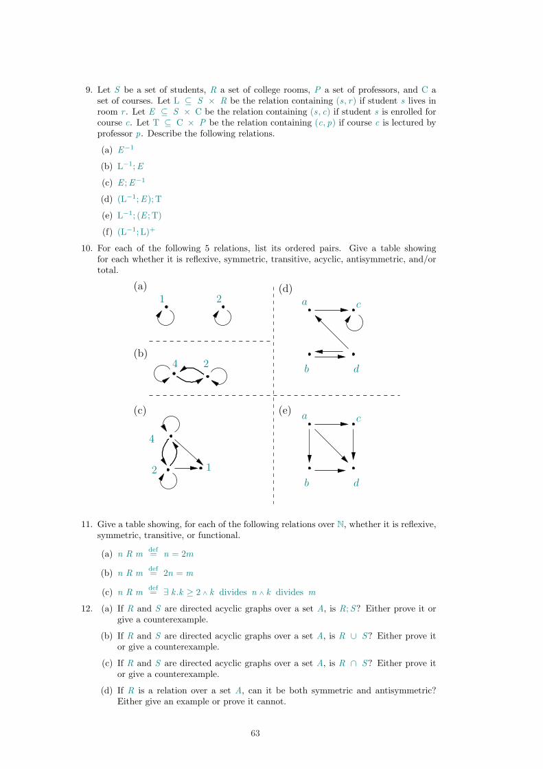
9. Let S be a set of students, R a set of college rooms, P a set of professors, and C aset of courses. Let L ⊆ S × R be the relation containing (s, r) if student s lives inroom r . Let E ⊆ S × C be the relation containing (s, c) if student s is enrolled forcourse c. Let T ⊆ C × P be the relation containing (c, p) if course c is lectured byprofessor p. Describe the following relations.
(a) E−1
(b) L−1;E
(c) E ;E−1
(d) (L−1;E ); T
(e) L−1; (E ; T)
(f) (L−1; L)+
10. For each of the following 5 relations, list its ordered pairs. Give a table showingfor each whether it is reflexive, symmetric, transitive, acyclic, antisymmetric, and/ortotal.
c
db
a
c
db
a
2
4
1
24
21(a)
(b)
(c) (e)
(d)
11. Give a table showing, for each of the following relations over N, whether it is reflexive,symmetric, transitive, or functional.
(a) n R mdef= n = 2m
(b) n R mdef= 2n = m
(c) n R mdef= ∃ k .k ≥ 2 ∧ k divides n ∧ k divides m
12. (a) If R and S are directed acyclic graphs over a set A, is R;S? Either prove it orgive a counterexample.
(b) If R and S are directed acyclic graphs over a set A, is R ∪ S? Either prove itor give a counterexample.
(c) If R and S are directed acyclic graphs over a set A, is R ∩ S? Either prove itor give a counterexample.
(d) If R is a relation over a set A, can it be both symmetric and antisymmetric?Either give an example or prove it cannot.
63
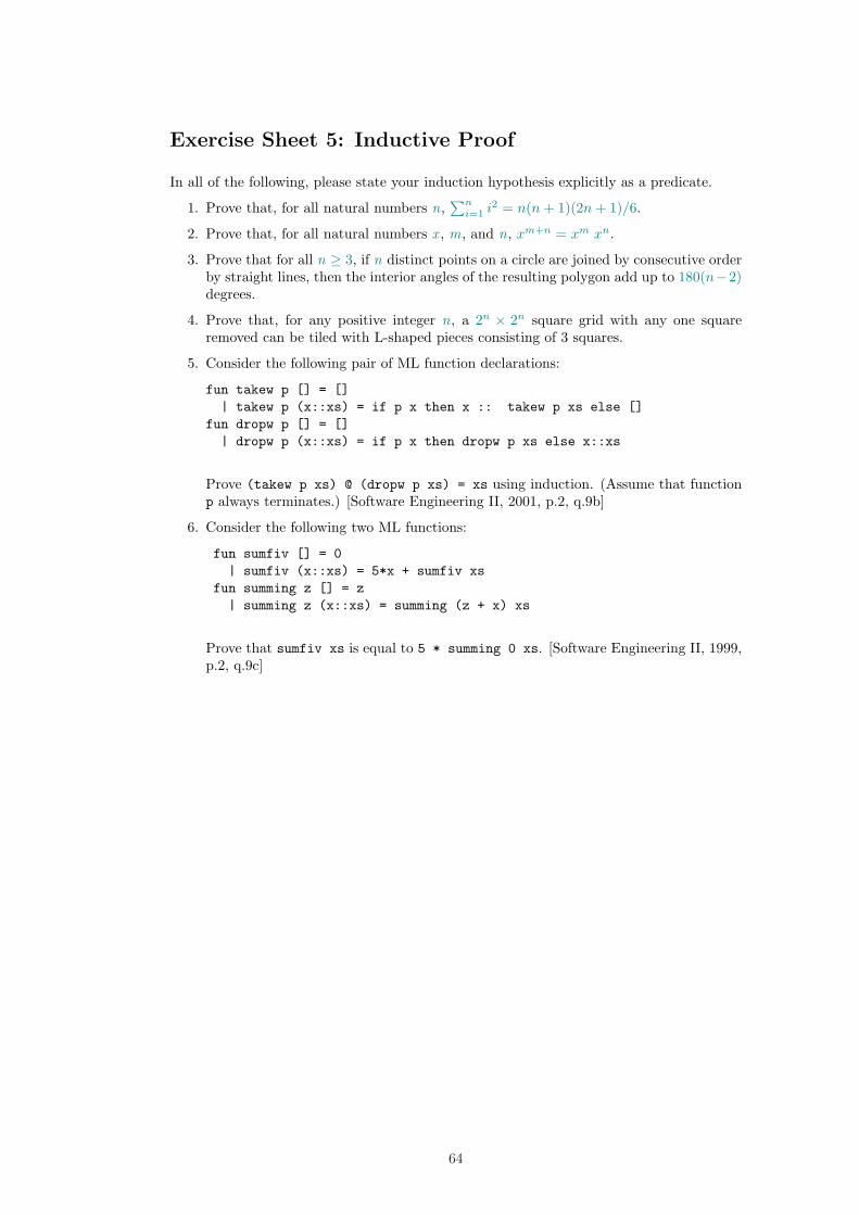
Exercise Sheet 5: Inductive Proof
In all of the following, please state your induction hypothesis explicitly as a predicate.
1. Prove that, for all natural numbers n,∑n
i=1 i2 = n(n + 1)(2n + 1)/6.
2. Prove that, for all natural numbers x , m, and n, xm+n = xm xn.
3. Prove that for all n ≥ 3, if n distinct points on a circle are joined by consecutive orderby straight lines, then the interior angles of the resulting polygon add up to 180(n−2)degrees.
4. Prove that, for any positive integer n, a 2n × 2n square grid with any one squareremoved can be tiled with L-shaped pieces consisting of 3 squares.
5. Consider the following pair of ML function declarations:
fun takew p [] = []
| takew p (x::xs) = if p x then x :: takew p xs else []
fun dropw p [] = []
| dropw p (x::xs) = if p x then dropw p xs else x::xs
Prove (takew p xs) @ (dropw p xs) = xs using induction. (Assume that functionp always terminates.) [Software Engineering II, 2001, p.2, q.9b]
6. Consider the following two ML functions:
fun sumfiv [] = 0
| sumfiv (x::xs) = 5*x + sumfiv xs
fun summing z [] = z
| summing z (x::xs) = summing (z + x) xs
Prove that sumfiv xs is equal to 5 * summing 0 xs. [Software Engineering II, 1999,p.2, q.9c]
64
![[ Philippe Salembier and Michael H.F. Wilkinson ] Connected Operatorsmichael/IEEE_SPM_2009_Salembier_Wilkinson.pdf · 2010-01-18 · complete lattice theory [29], [30] that are going](https://img.dokumen.tips/doc/110x75/5ea8370f90655e5f3e7beb95/-philippe-salembier-and-michael-hf-wilkinson-connected-michaelieeespm2009salembierwilkinsonpdf.jpg)