Embed Size (px)
Citation preview

Discrete Mathematics
i

Discrete Mathematics
Table of Contents
About the Tutorial ............................................................................................................................................ i
Audience........................................................................................................................................................... i Prerequisites..................................................................................................................................................... i Copyright & Disclaimer..................................................................................................................................... i
Table of Contents ............................................................................................................................................ ii
1. Discrete Mathematics – Introduction........................................................................................................ 1
Topics in Discrete Mathematics ...................................................................................................................... 1
PART 1: SETS, RELATIONS, AND FUNCTIONS ............................................................................... 2
2. Sets ........................................................................................................................................................... 3
Set – Definition ................................................................................................................................................ 3
Representation of a Set.................................................................................................................................. 3
Cardinality of a Set .......................................................................................................................................... 4
Types of Sets.................................................................................................................................................... 4
Venn Diagrams ................................................................................................................................................ 6 Set Operations................................................................................................................................................. 7
Power Set ........................................................................................................................................................ 8 Partitioning of a Set ......................................................................................................................................... 9
3. Relations................................................................................................................................................. 10 Definition and Properties .............................................................................................................................. 10 Domain and Range ........................................................................................................................................ 10
Representation of Relations using Graph...................................................................................................... 10 Types of Relations ......................................................................................................................................... 11
4. Functions ................................................................................................................................................ 12 Function – Definition ..................................................................................................................................... 12 Injective / One-to-one function..................................................................................................................... 12
Surjective / Onto function ............................................................................................................................. 12 Bijective / One-to-one Correspondent .......................................................................................................... 12
Composition of Functions.............................................................................................................................. 13
PART 2: MATHEMATICAL LOGIC................................................................................................ 14
5. Propositional Logic.................................................................................................................................. 15
Prepositional Logic – Definition..................................................................................................................... 15
Connectives ................................................................................................................................................... 15 Tautologies .................................................................................................................................................... 17
Contradictions ............................................................................................................................................... 17
Contingency................................................................................................................................................... 17
Propositional Equivalences............................................................................................................................ 18 Inverse, Converse, and Contra-positive........................................................................................................ 18
Duality Principle............................................................................................................................................ 19
Normal Forms................................................................................................................................................ 19
ii
Discrete Mathematics
6. Predicate Logic........................................................................................................................................ 20
Predicate Logic – Definition........................................................................................................................... 20
Well Formed Formula.................................................................................................................................... 20
Quantifiers..................................................................................................................................................... 20 Nested Quantifiers ........................................................................................................................................ 21
7. Rules of Inference ................................................................................................................................... 22
What are Rules of Inference for? .................................................................................................................. 22
Addition ......................................................................................................................................................... 22
Conjunction ................................................................................................................................................... 22 Simplification ................................................................................................................................................. 23
Modus Ponens............................................................................................................................................... 23
Modus Tollens ............................................................................................................................................... 23
Disjunctive Syllogism ..................................................................................................................................... 24 Hypothetical Syllogism .................................................................................................................................. 24
Constructive Dilemma ................................................................................................................................... 24
Destructive Dilemma ..................................................................................................................................... 25
PART 3: GROUP THEORY ........................................................................................................... 26
8. Operators and Postulates ....................................................................................................................... 27
Closure........................................................................................................................................................... 27
Associative Laws ............................................................................................................................................ 27
Commutative Laws ........................................................................................................................................ 28
Distributive Laws ........................................................................................................................................... 28 Identity Element ............................................................................................................................................ 28
Inverse ........................................................................................................................................................... 29 De Morgan’s Law ........................................................................................................................................... 29
9. Group Theory.......................................................................................................................................... 30 Semigroup ..................................................................................................................................................... 30
Monoid .......................................................................................................................................................... 30 Group............................................................................................................................................................. 30
Abelian Group................................................................................................................................................ 31
Cyclic Group and Subgroup ........................................................................................................................... 31 Partially Ordered Set (POSET)........................................................................................................................ 32
Hasse Diagram ............................................................................................................................................... 32
Linearly Ordered Set...................................................................................................................................... 33
Lattice ............................................................................................................................................................ 33 Properties of Lattices..................................................................................................................................... 35
Dual of a Lattice............................................................................................................................................. 35
PART 4: COUNTING & PROBABILITY .......................................................................................... 36
10. Counting Theory ..................................................................................................................................... 37
The Rules of Sum and Product ...................................................................................................................... 37 Permutations ................................................................................................................................................. 37
Combinations ................................................................................................................................................ 39 Pascal's Identity ............................................................................................................................................. 40
Pigeonhole Principle...................................................................................................................................... 40 The Inclusion-Exclusion principle .................................................................................................................. 41
iii
Discrete Mathematics
11. Probability .............................................................................................................................................. 42
Basic Concepts............................................................................................................................................... 42
Probability Axioms......................................................................................................................................... 43
Properties of Probability............................................................................................................................... 43 Conditional Probability .................................................................................................................................. 44
Bayes' Theorem ............................................................................................................................................. 45
PART 5: MATHEMATICAL INDUCTION & RECURRENCE RELATIONS ........................................... 47
12. Mathematical Induction......................................................................................................................... 48
Definition ....................................................................................................................................................... 48
How to Do It .................................................................................................................................................. 48 Strong Induction ............................................................................................................................................ 49
13. Recurrence Relation................................................................................................................................ 50
Definition ....................................................................................................................................................... 50 Linear Recurrence Relations.......................................................................................................................... 50 Particular Solutions ....................................................................................................................................... 52
Generating Functions .................................................................................................................................... 53
PART 6: DISCRETE STRUCTURES ................................................................................................ 55
14. Graph and Graph Models........................................................................................................................ 56 What is a Graph? ........................................................................................................................................... 56
Types of Graphs............................................................................................................................................. 57 Representation of Graphs ............................................................................................................................. 60
Planar vs. Non-planar graph .......................................................................................................................... 62 Isomorphism.................................................................................................................................................. 63
Homomorphism............................................................................................................................................ 63
Euler Graphs .................................................................................................................................................. 63
Hamiltonian Graphs....................................................................................................................................... 64
15. More on Graphs...................................................................................................................................... 66
Graph Coloring .............................................................................................................................................. 66
Graph Traversal ............................................................................................................................................. 67
16. Introduction to Trees .............................................................................................................................. 71
Tree and its Properties .................................................................................................................................. 71 Centers and Bi-Centers of a Tree................................................................................................................... 71 Labeled Trees ................................................................................................................................................ 74
Unlabeled trees............................................................................................................................................. 74
Rooted Tree ................................................................................................................................................... 75 Binary Search Tree......................................................................................................................................... 76
17. Spanning Trees....................................................................................................................................... 78 Minimum Spanning Tree ............................................................................................................................... 79
Kruskal's Algorithm........................................................................................................................................ 79
Prim's Algorithm ............................................................................................................................................ 82
iv

Discrete Mathematics
PART 7: BOOLEAN ALGEBRA ..................................................................................................... 86
18. Boolean Expressions and Functions ........................................................................................................ 87
Boolean Functions ......................................................................................................................................... 87
Boolean Expressions...................................................................................................................................... 87 Boolean Identities......................................................................................................................................... 87
Canonical Forms ............................................................................................................................................ 88
Logic Gates .................................................................................................................................................... 90
19. Simplification of Boolean Functions ........................................................................................................ 93 Simplification Using Algebraic Functions....................................................................................................... 93
Karnaugh Maps............................................................................................................................................. 94
Simplification Using K- map........................................................................................................................... 95
v

1. DISCRETE MATHEMATICS – INTRODUCTION
Discrete Mathematics
Mathematics can be broadly classified into two categories:
Continuous Mathematics
Discrete Mathematics
Continuous Mathematics is based upon continuous number line or the real numbers. It
is characterized by the fact that between any two numbers, there are almost always an infinite set of numbers. For example, a function in continuous mathematics can be plotted in a smooth curve without breaks.
Discrete Mathematics, on the other hand, involves distinct values; i.e. between any two
points, there are a countable number of points. For example, if we have a finite set of objects, the function can be defined as a list of ordered pairs having these objects, and can be presented as a complete list of those pairs.
Topics in Discrete Mathematics
Though there cannot be a definite number of branches of Discrete Mathematics, the
following topics are almost always covered in any study regarding this matter:
Sets, Relations and Functions
Mathematical Logic
Group theory Counting Theory Probability Mathematical Induction and Recurrence Relations
Graph Theory
Trees Boolean Algebra
1

Discrete Mathematics
Part 1: Sets, Relations, and Functions
2

2. SETS Discrete Mathematics
German mathematician G. Cantor introduced the concept of sets. He had defined a set as a collection of definite and distinguishable objects selected by the means of certain rules or description.
Set theory forms the basis of several other fields of study like counting theory, relations,
graph theory and finite state machines. In this chapter, we will cover the different aspects of Set Theory.
Set – Definition
A set is an unordered collection of different elements. A set can be written explicitly by
listing its elements using set bracket. If the order of the elements is changed or any element of a set is repeated, it does not make any changes in the set.
Some Example of Sets
A set of all positive integers
A set of all the planets in the solar system
A set of all the states in India
A set of all the lowercase letters of the alphabet
Representation of a Set
Sets can be represented in two ways:
Roster or Tabular Form
Set Builder Notation
Roster or Tabular Form
The set is represented by listing all the elements comprising it. The elements are enclosed
within braces and separated by commas.
Example 1: Set of vowels in English alphabet, A = {a,e,i,o,u}
Example 2: Set of odd numbers less than 10, B = {1,3,5,7,9}
Set Builder Notation
The set is defined by specifying a property that elements of the set have in common. The
set is described as A = { x : p(x)}
Example 1: The set {a,e,i,o,u} is written as:
A = { x : x is a vowel in English alphabet}
3

Discrete Mathematics
Example 2: The set {1,3,5,7,9} is written as:
B = { x : 1≤x<10 and (x%2) ≠ 0}
If an element x is a member of any set S, it is denoted by x∈ S and if an element y is not
a member of set S, it is denoted by y ∉ S.
Example: If S = {1, 1.2,1.7,2}, 1∈ S but 1.5 ∉S
Some Important Sets
N: the set of all natural numbers = {1, 2, 3, 4, .....}
Z: the set of all integers = {....., -3, -2, -1, 0, 1, 2, 3, .....} Z+: the set of all positive integers Q: the set of all rational numbers R: the set of all real numbers W: the set of all whole numbers
Cardinality of a Set
Cardinality of a set S, denoted by |S|, is the number of elements of the set. If a set has
an infinite number of elements, its cardinality is ∞.
Example: |{1, 4, 3,5}| = 4, |{1, 2, 3,4,5,…}| = ∞
If there are two sets X and Y,
| X| = | Y | represents two sets X and Y that have the same cardinality, if there
exists a bijective function „f‟ from X to Y.
| X| ≤ | Y | represents set X has cardinality less than or equal to the cardinality of
Y, if there exists an injective function „f‟ from X to Y.
| X| < | Y | represents set X has cardinality less than the cardinality of Y, if there is
an injective function f, but no bijective function „f‟ from X to Y.
If | X | ≤ | Y | and | X | ≤ | Y | then | X | = | Y |
Types of Sets
Sets can be classified into many types. Some of which are finite, infinite, subset, universal,
proper, singleton set, etc.
4

Discrete Mathematics
Finite Set
A set which contains a definite number of elements is called a finite set.
Example: S = {x | x ∈ N and 70 > x > 50}
Infinite Set
A set which contains infinite number of elements is called an infinite set.
Example: S = {x | x ∈ N and x > 10}
Subset
A set X is a subset of set Y (Written as X ⊆ Y) if every element of X is an element of set Y.
Example 1: Let, X = { 1, 2, 3, 4, 5, 6 } and Y = { 1, 2 }. Here set Y is a subset of set X as all the elements of set Y is in set X. Hence, we can write Y ⊆ X.
Example 2: Let, X = {1, 2, 3} and Y = {1, 2, 3}. Here set Y is a subset (Not a proper subset) of set X as all the elements of set Y is in set X. Hence, we can write Y ⊆ X.
Proper Subset
The term “proper subset” can be defined as “subset of but not equal to”. A Set X is a
proper subset of set Y (Written as X ⊂ Y) if every element of X is an element of set Y and | X| < | Y |. Example: Let, X = {1, 2,3,4,5, 6} and Y = {1, 2}. Here set Y is a proper subset of set X as at least one element is more in set X. Hence, we can write Y ⊂ X.
Universal Set
It is a collection of all elements in a particular context or application. All the sets in that
context or application are essentially subsets of this universal set. Universal sets are
represented as U.
Example: We may define U as the set of all animals on earth. In this case, set of all
mammals is a subset of U, set of all fishes is a subset of U, set of all insects is a subset
of U, and so on.
Empty Set or Null Set
An empty set contains no elements. It is denoted by ∅. As the number of elements in an
empty set is finite, empty set is a finite set. The cardinality of empty set or null set is zero.
Example: ∅ = {x | x ∈ N and 7 < x < 8}
5

Discrete Mathematics
Singleton Set or Unit Set
Singleton set or unit set contains only one element. A singleton set is denoted by {s}.
Example: S = {x | x ∈ N, 7 < x < 9}
Equal Set
If two sets contain the same elements they are said to be equal.
Example: If A = {1, 2, 6} and B = {6, 1, 2}, they are equal as every element of set A is an element of set B and every element of set B is an element of set A.
Equivalent Set
If the cardinalities of two sets are same, they are called equivalent sets.
Example: If A = {1, 2, 6} and B = {16, 17, 22}, they are equivalent as cardinality of A is equal to the cardinality of B. i.e. |A|=|B|=3
Overlapping Set
Two sets that have at least one common element are called overlapping sets.
In case of overlapping sets:
n(A ∪ B) = n(A) + n(B) - n(A ∩ B)
n(A ∪ B) = n(A - B) + n(B - A) + n(A ∩ B)
n(A) = n(A - B) + n(A ∩ B)
n(B) = n(B - A) + n(A ∩ B)
Example: Let, A = {1, 2, 6} and B = {6, 12, 42}. There is a common element „6‟, hence these sets are overlapping sets.
Disjoint Set
If two sets C and D are disjoint sets as they do not have even one element in common.
Therefore, n(A ∪ B) = n(A) + n(B)
Example: Let, A = {1, 2, 6} and B = {7, 9, 14}, there is no common element, hence these sets are overlapping sets.
Venn Diagrams
Venn diagram, invented in1880 by John Venn, is a schematic diagram that shows all
possible logical relations between different mathematical sets.
6

Discrete Mathematics
Examples
Set Operations
Set Operations include Set Union, Set Intersection, Set Difference, Complement of Set,
and Cartesian Product.
Set Union
The union of sets A and B (denoted by A ∪ B) is the set of elements which are in A, in B,
or in both A and B. Hence, A∪B = {x | x ∈A OR x ∈B}.
Example: If A = {10, 11, 12, 13} and B = {13, 14, 15}, then A ∪ B = {10, 11, 12, 13,
14, 15}. (The common element occurs only once)
A B
Figure: Venn Diagram of A ∪ B
Set Intersection
The intersection of sets A and B (denoted by A ∩ B) is the set of elements which are in
both A and B. Hence, A∩B = {x | x ∈A AND x ∈B}.
Example: If A = {11, 12, 13} and B = {13, 14, 15}, then A∩B = {13}.
A
B
Figure: Venn Diagram of A ∩ B
7
A
Discrete Mathematics
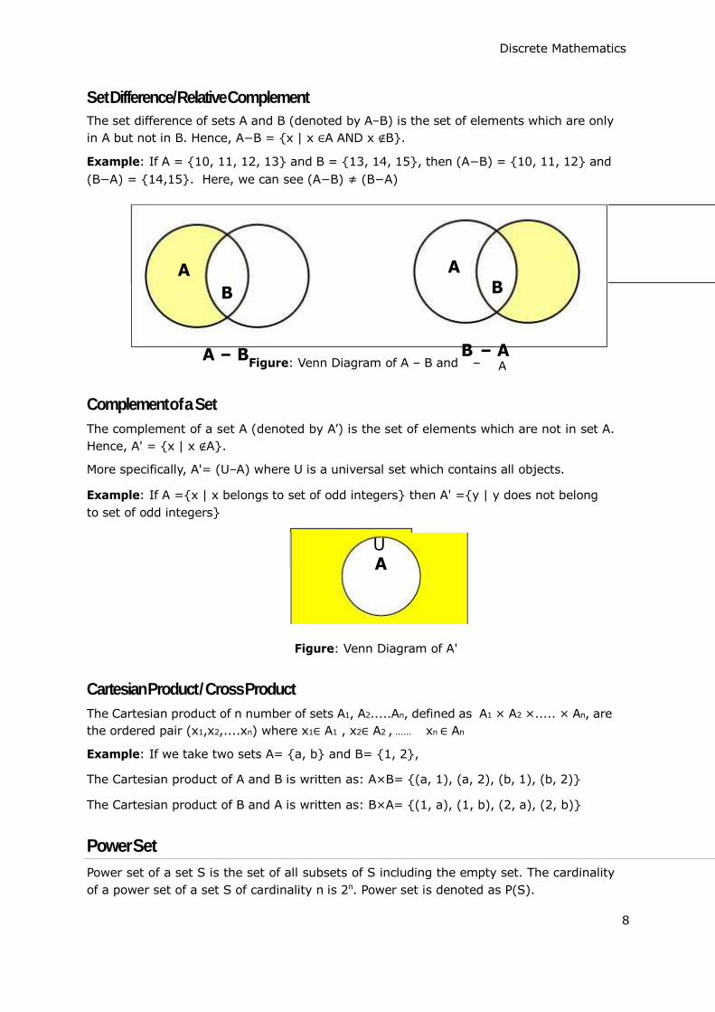
Set Difference/ Relative Complement
The set difference of sets A and B (denoted by A–B) is the set of elements which are only
in A but not in B. Hence, A−B = {x | x ∈A AND x ∉B}.
Example: If A = {10, 11, 12, 13} and B = {13, 14, 15}, then (A−B) = {10, 11, 12} and
(B−A) = {14,15}. Here, we can see (A−B) ≠ (B−A)
A
B
A
B
A – BFigure: Venn Diagram of A – B and B––
A
Complement of a Set
The complement of a set A (denoted by A‟) is the set of elements which are not in set A.
Hence, A' = {x | x ∉A}.
More specifically, A'= (U–A) where U is a universal set which contains all objects.
Example: If A ={x | x belongs to set of odd integers} then A' ={y | y does not belong
to set of odd integers}
U
A
Figure: Venn Diagram of A'
Cartesian Product / Cross Product
The Cartesian product of n number of sets A1, A2.....An, defined as A1 × A2 ×..... × An, are
the ordered pair (x1,x2,....xn) where x1∈ A1 , x2∈ A2 , ...... xn ∈ An
Example: If we take two sets A= {a, b} and B= {1, 2},
The Cartesian product of A and B is written as: A×B= {(a, 1), (a, 2), (b, 1), (b, 2)}
The Cartesian product of B and A is written as: B×A= {(1, a), (1, b), (2, a), (2, b)}
Power Set
Power set of a set S is the set of all subsets of S including the empty set. The cardinality
of a power set of a set S of cardinality n is 2n. Power set is denoted as P(S).
8

Discrete Mathematics
Example:
For a set S = {a, b, c, d} let us calculate the subsets:
Subsets with 0 elements: {∅} (the empty set)
Subsets with 1 element: {a}, {b}, {c}, {d} Subsets with 2 elements: {a,b}, {a,c}, {a,d}, {b,c}, {b,d},{c,d}
Subsets with 3 elements: {a,b,c},{a,b,d},{a,c,d},{b,c,d} Subsets with 4 elements: {a,b,c,d}
Hence, P(S) =
{ {∅},{a}, {b}, {c}, {d},{a,b}, {a,c}, {a,d}, {b,c},
{b,d},{c,d},{a,b,c},{a,b,d},{a,c,d},{b,c,d},{a,b,c,d} }
| P(S) | = 24 =16
Note: The power set of an empty set is also an empty set.
| P ({∅}) | = 20 = 1
Partitioning of a Set
Partition of a set, say S, is a collection of n disjoint subsets, say P1, P2,...… Pn, that satisfies
the following three conditions:
Pi does not contain the empty set.
[ Pi ≠ {∅} for all 0 < i ≤ n]
The union of the subsets must equal the entire original set.
[P1 ∪ P2 ∪ ..... ∪ Pn = S]
The intersection of any two distinct sets is empty.
[Pa ∩ Pb ={∅}, for a ≠ b where n ≥ a, b ≥ 0 ]
The number of partitions of the set is called a Bell number denoted as Bn.
Example
Let S = {a, b, c, d, e, f, g, h}
One probable partitioning is {a}, {b, c, d}, {e, f, g,h}
Another probable partitioning is {a,b}, { c, d}, {e, f, g,h}
In this way, we can find out Bn number of different partitions.
9
3. RELATIONS Discrete Mathematics
Whenever sets are being discussed, the relationship between the elements of the sets is
the next thing that comes up. Relations may exist between objects of the same set or
between objects of two or more sets.
Definition and Properties
A binary relation R from set x to y (written as xRy or R(x,y)) is a subset of the Cartesian
product x × y. If the ordered pair of G is reversed, the relation also changes.
Generally an n-ary relation R between sets A1, ... , and An is a subset of the n-ary product
A1×...×An. The minimum cardinality of a relation R is Zero and maximum is n2 in this case.
A binary relation R on a single set A is a subset of A × A.
For two distinct sets, A and B, having cardinalities m and n respectively, the maximum
cardinality of a relation R from A to B is mn.
Domain and Range
If there are two sets A and B, and relation R have order pair (x, y), then:
The domain of R is the set { x | (x, y) ∈ R for some y in B }
The range of R is the set { y | (x, y) ∈ R for some x in A }
Examples
Let, A = {1,2,9} and B = {1,3,7}
Case 1: If relation R is „equal to‟ then R = {(1, 1), (3, 3)}
Case 2: If relation R is „less than‟ then R = {(1, 3), (1, 7), (2, 3), (2, 7)}
Case 3: If relation R is „greater than‟ then R = {(2, 1), (9, 1), (9, 3), (9, 7)}
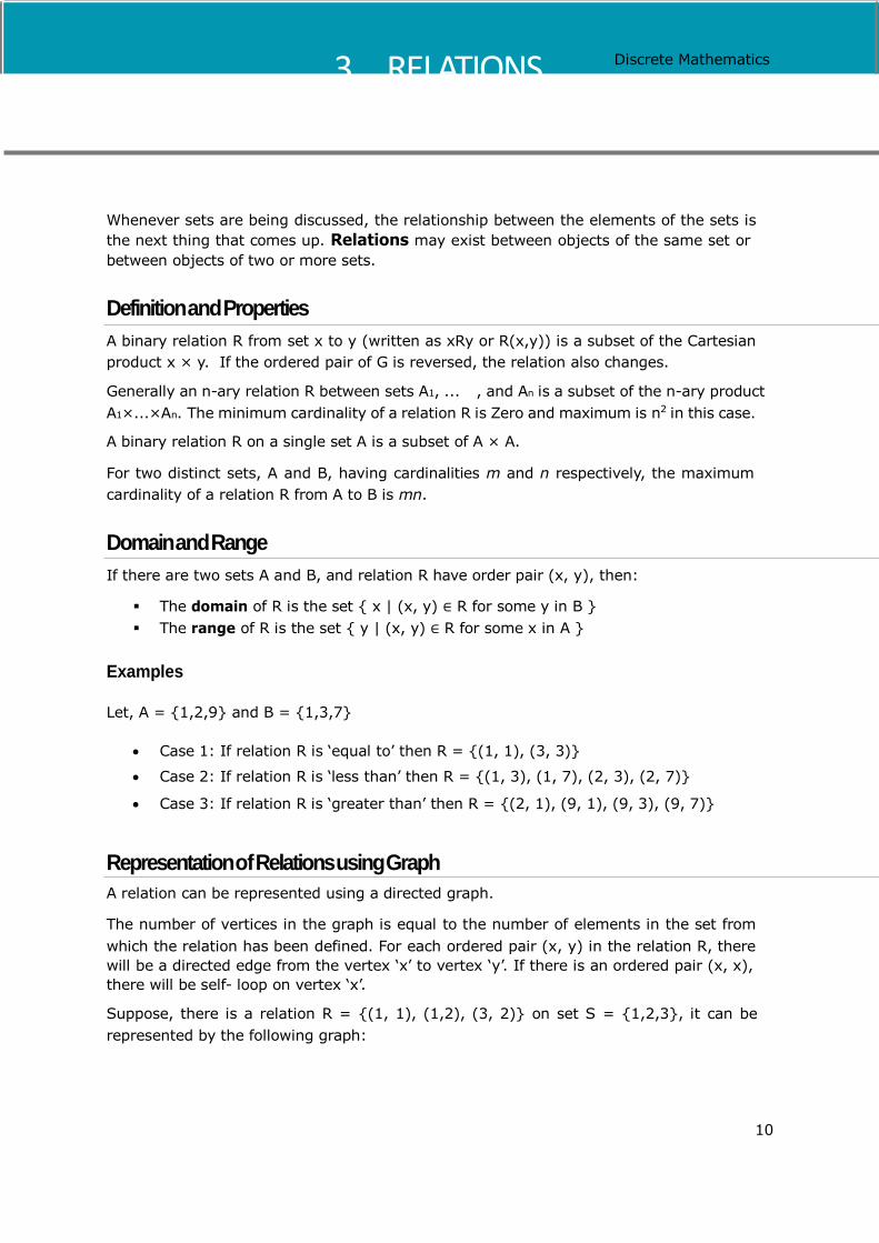
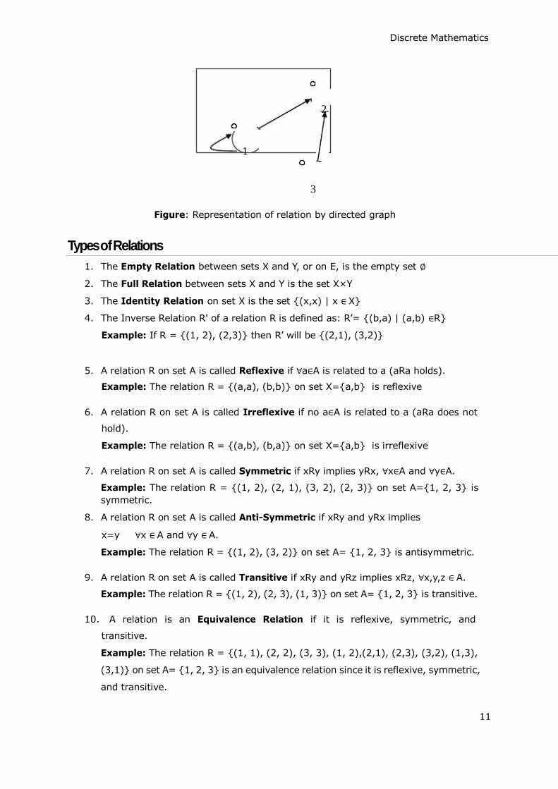
Representation of Relations using Graph
A relation can be represented using a directed graph.
The number of vertices in the graph is equal to the number of elements in the set from
which the relation has been defined. For each ordered pair (x, y) in the relation R, there will be a directed edge from the vertex „x‟ to vertex „y‟. If there is an ordered pair (x, x), there will be self- loop on vertex „x‟.
Suppose, there is a relation R = {(1, 1), (1,2), (3, 2)} on set S = {1,2,3}, it can be
represented by the following graph:
10
Discrete Mathematics
2
1
3
Figure: Representation of relation by directed graph
Types of Relations
1. The Empty Relation between sets X and Y, or on E, is the empty set ∅
2. The Full Relation between sets X and Y is the set X×Y
3. The Identity Relation on set X is the set {(x,x) | x ∈ X}
4. The Inverse Relation R' of a relation R is defined as: R‟= {(b,a) | (a,b) ∈R}
Example: If R = {(1, 2), (2,3)} then R‟ will be {(2,1), (3,2)}
5. A relation R on set A is called Reflexive if ∀a∈A is related to a (aRa holds).
Example: The relation R = {(a,a), (b,b)} on set X={a,b} is reflexive
6. A relation R on set A is called Irreflexive if no a∈A is related to a (aRa does not
hold).
Example: The relation R = {(a,b), (b,a)} on set X={a,b} is irreflexive
7. A relation R on set A is called Symmetric if xRy implies yRx, ∀x∈A and ∀y∈A.
Example: The relation R = {(1, 2), (2, 1), (3, 2), (2, 3)} on set A={1, 2, 3} is
symmetric.
8. A relation R on set A is called Anti-Symmetric if xRy and yRx implies
x=y ∀x ∈ A and ∀y ∈ A.
Example: The relation R = {(1, 2), (3, 2)} on set A= {1, 2, 3} is antisymmetric.
9. A relation R on set A is called Transitive if xRy and yRz implies xRz, ∀x,y,z ∈ A.
Example: The relation R = {(1, 2), (2, 3), (1, 3)} on set A= {1, 2, 3} is transitive.
10. A relation is an Equivalence Relation if it is reflexive, symmetric, and
transitive.
Example: The relation R = {(1, 1), (2, 2), (3, 3), (1, 2),(2,1), (2,3), (3,2), (1,3),
(3,1)} on set A= {1, 2, 3} is an equivalence relation since it is reflexive, symmetric,
and transitive.
11

4. FUNCTIONS Discrete Mathematics
A Function assigns to each element of a set, exactly one element of a related set. Functions find their application in various fields like representation of the computational complexity of algorithms, counting objects, study of sequences and strings, to name a few. The third and final chapter of this part highlights the important aspects of functions.
Function – Definition
A function or mapping (Defined as f: X→Y) is a relationship from elements of one set X to
elements of another set Y (X and Y are non-empty sets). X is called Domain and Y is called Codomain of function „f‟.
Function „f‟ is a relation on X and Y s.t for each x ∈X, there exists a unique y ∈ Y such that
(x,y) ∈ R. x is called pre-image and y is called image of function f.
A function can be one to one, many to one (not one to many). A function f: A→B is said
to be invertible if there exists a function g: B→A
Injective / One-to-one function
A function f: A→B is injective or one-to-one function if for every b ∈ B, there exists at most
one a ∈ A such that f(s) = t.
This means a function f is injective if a1 ≠ a2 implies f(a1) ≠ f(a2).
Example
1. f: N →N, f(x) = 5x is injective.
2. f: Z+→Z+, f(x) = x2 is injective.
3. f: N→N, f(x) = x2 is not injective as (-x)2 = x2
Surjective / Onto function
A function f: A →B is surjective (onto) if the image of f equals its range. Equivalently, for
every b ∈ B, there exists some a ∈ A such that f(a) = b. This means that for any y in B, there exists some x in A such that y = f(x).
Example
1. f : Z+→Z+, f(x) = x2 is surjective.
2. f : N→N, f(x) = x2 is not injective as (-x)2 = x2
Bijective / One-to-one Correspondent
A function f: A →B is bijective or one-to-one correspondent if and only if f is both injective
and surjective.
12
Discrete Mathematics
Problem:
Prove that a function f: R→R defined by f(x) = 2x – 3 is a bijective function.
Explanation: We have to prove this function is both injective and surjective.
If f(x1) = f(x2), then 2x1 – 3 = 2x2 – 3 and it implies that x1 = x2.
Hence, f is injective.
Here, 2x – 3= y
So, x = (y+5)/3 which belongs to R and f(x) = y.
Hence, f is surjective.
Since f is both surjective and injective, we can say f is bijective.
Composition of Functions
Two functions f: A→B and g: B→C can be composed to give a composition g o f. This is a
function from A to C defined by (gof)(x) = g(f(x))
Example
Let f(x) = x + 2 and g(x) = 2x, find ( f o g)(x) and ( g o f)(x)
Solution
(f o g)(x) = f (g(x)) = f(2x) = 2x+2
(g o f)(x) = g (f(x)) = g(x+2) = 2(x+2)=2x+4
Hence, (f o g)(x) ≠ (g o f)(x)
Some Facts about Composition
If f and g are one-to-one then the function (g o f) is also one-to-one.
If f and g are onto then the function (g o f) is also onto.
Composition always holds associative property but does not hold commutative
property.
13
Discrete Mathematics
Part 2: Mathematical Logic
14

5. PROPOSITIONAL LOGIC
Discrete Mathematics
The rules of mathematical logic specify methods of reasoning mathematical statements. Greek philosopher, Aristotle, was the pioneer of logical reasoning. Logical reasoning provides the theoretical base for many areas of mathematics and consequently computer
science. It has many practical applications in computer science like design of computing machines, artificial intelligence, definition of data structures for programming languages etc.
Propositional Logic is concerned with statements to which the truth values, “true” and
“false”, can be assigned. The purpose is to analyze these statements either individually or in a composite manner.
Prepositional Logic – Definition
A proposition is a collection of declarative statements that has either a truth value "true”
or a truth value "false". A propositional consists of propositional variables and connectives. We denote the propositional variables by capital letters (A, B, etc). The connectives connect the propositional variables.
Some examples of Propositions are given below:
"Man is Mortal", it returns truth value “TRUE”
"12 + 9 = 3 – 2", it returns truth value “FALSE”
The following is not a Proposition:
"A is less than 2". It is because unless we give a specific value of A, we cannot say
whether the statement is true or false.
Connectives
In propositional logic generally we use five connectives which are: OR (V), AND (Λ),
Negation/ NOT (¬), Implication / if-then (→), If and only if (⇔).
OR (V): The OR operation of two propositions A and B (written as A V B) is true if at least
any of the propositional variable A or B is true.
The truth table is as follows:
AND (Λ): The AND operation of two propositions A and B (written as A Λ B) is true if both the propositional variable A and B is true.
15
A B AVB
True True True
True False True
False True True
False False False
Discrete Mathematics
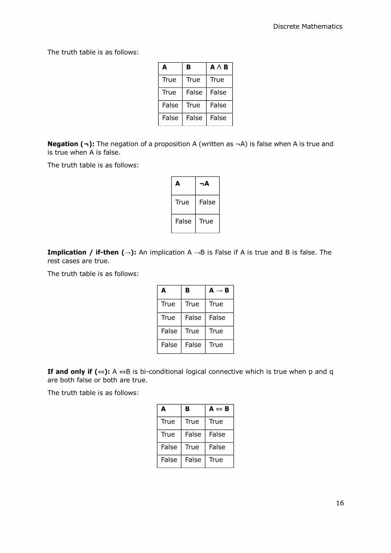
The truth table is as follows:
Negation (¬): The negation of a proposition A (written as ¬A) is false when A is true and is true when A is false.
The truth table is as follows:
Implication / if-then (→): An implication A →B is False if A is true and B is false. The rest cases are true.
The truth table is as follows:
If and only if (⇔): A ⇔B is bi-conditional logical connective which is true when p and q are both false or both are true.
The truth table is as follows:
16
A B A → B
True True True
True False False
False True True
False False True
A B A ⇔ B
True True True
True False False
False True False
False False True
A B A Λ B
True True True
True False False
False True False
False False False
A ¬A
True False
False True
The truth table is as follows:
The truth table is as follows:
The truth table is as follows:
Discrete Mathematics
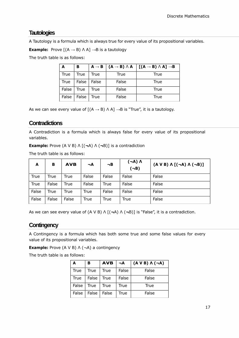
Tautologies
A Tautology is a formula which is always true for every value of its propositional variables.
Example: Prove [(A → B) Λ A] →B is a tautology
As we can see every value of [(A → B) Λ A] →B is “True”, it is a tautology.
Contradictions
A Contradiction is a formula which is always false for every value of its propositional
variables.
Example: Prove (A V B) Λ [(¬A) Λ (¬B)] is a contradiction
As we can see every value of (A V B) Λ [(¬A) Λ (¬B)] is “False”, it is a contradiction.
Contingency
A Contingency is a formula which has both some true and some false values for every
value of its propositional variables.
Example: Prove (A V B) Λ (¬A) a contingency
17
A B AVB ¬A ¬B (¬A) Λ
(¬B) (A V B) Λ [(¬A) Λ (¬B)]
True True True False False False False
True False True False True False False
False True True True False False False
False False False True True True False
A B A → B (A → B) Λ A [(A → B) Λ A] →B
True True True True True
True False False False True
False True True False True
False False True False True
A B AVB ¬A (A V B) Λ (¬A)
True True True False False
True False True False False
False True True True True
False False False True False

Testing by 1st method (Matching truth table):
Testing by 2nd method (Bi-conditionality):
Discrete Mathematics
As we can see every value of (A V B) Λ (¬A) has both “True” and “False”, it is a
contingency.
Propositional Equivalences
Two statements X and Y are logically equivalent if any of the following two conditions hold:
The truth tables of each statement have the same truth values.
The bi-conditional statement X ⇔ Y is a tautology.
Example: Prove ¬ (A V B) and [(¬A) Λ (¬B)] are equivalent
Here, we can see the truth values of ¬ (A V B) and [(¬A) Λ (¬B)] are same, hence the statements are equivalent.
As [¬ (A V B)] ⇔ [(¬A) Λ (¬B)] is a tautology, the statements are equivalent.
Inverse, Converse, and Contra-positive
A conditional statement has two parts: Hypothesis and Conclusion.
Example of Conditional Statement: “If you do your homework, you will not be
punished.” Here, "you do your homework" is the hypothesis and "you will not be punished"
is the conclusion.
Inverse: An inverse of the conditional statement is the negation of both the hypothesis
and the conclusion. If the statement is “If p, then q”, the inverse will be “If not p, then not q”. The inverse of “If you do your homework, you will not be punished” is “If you do not do your homework, you will be punished.”
18
A B ¬ (A V B) [(¬A) Λ (¬B)] [¬ (A V B)] ⇔[(¬A) Λ (¬B)]
True True False False True
True False False False True
False True False False True
False False True True True
A B AVB ¬ (A V B) ¬A ¬B [(¬A) Λ (¬B)]
True True True False False False False
True False True False False True False
False True True False True False False
False False False True True True True

Discrete Mathematics
Converse: The converse of the conditional statement is computed by interchanging the
hypothesis and the conclusion. If the statement is “If p, then q”, the inverse will be “If q, then p”. The converse of "If you do your homework, you will not be punished" is "If you will not be punished, you do not do your homework”.
Contra-positive: The contra-positive of the conditional is computed by interchanging the
hypothesis and the conclusion of the inverse statement. If the statement is “If p, then q”, the inverse will be “If not q, then not p”. The Contra-positive of " If you do your homework, you will not be punished” is" If you will be punished, you do your homework”.
Duality Principle
Duality principle set states that for any true statement, the dual statement obtained by
interchanging unions into intersections (and vice versa) and interchanging Universal set
into Null set (and vice versa) is also true. If dual of any statement is the statement itself, it is said self-dual statement.
Example: The dual of (A ∩ B) ∪ C is (A∪ B) ∩ C
Normal Forms
We can convert any proposition in two normal forms:
Conjunctive normal form
Disjunctive normal form
Conjunctive Normal Form
A compound statement is in conjunctive normal form if it is obtained by operating AND
among variables (negation of variables included) connected with ORs. Examples
(P ∪Q) ∩ (Q ∪ R)
(¬P ∪Q ∪S ∪¬T)
Disjunctive Normal Form
A compound statement is in conjunctive normal form if it is obtained by operating OR
among variables (negation of variables included) connected with ANDs. Examples
(P ∩ Q) ∪ (Q ∩ R)
(¬P ∩Q ∩S ∩¬T)
19

6. PREDICATE LOGIC Discrete Mathematics
Predicate Logic deals with predicates, which are propositions containing variables.
Predicate Logic – Definition
A predicate is an expression of one or more variables defined on some specific domain. A
predicate with variables can be made a proposition by either assigning a value to the variable or by quantifying the variable.
The following are some examples of predicates:
Let E(x, y) denote "x = y"
Let X(a , b, c) denote "a + b + c = 0" Let M(x, y) denote "x is married to y"
Well Formed Formula
Well Formed Formula (wff) is a predicate holding any of the following -
All propositional constants and propositional variables are wffs
If x is a variable and Y is a wff, ∀x Y and ∃x Y are also wff
Truth value and false values are wffs
Each atomic formula is a wff
All connectives connecting wffs are wffs
Quantifiers
The variable of predicates is quantified by quantifiers. There are two types of quantifier in
predicate logic: Universal Quantifier and Existential Quantifier.
Universal Quantifier
Universal quantifier states that the statements within its scope are true for every value of
the specific variable. It is denoted by the symbol ∀.
∀x P(x) is read as for every value of x, P(x) is true.
Example: "Man is mortal" can be transformed into the propositional form ∀x P(x) where
P(x) is the predicate which denotes x is mortal and the universe of discourse is all men.
Existential Quantifier
Existential quantifier states that the statements within its scope are true for some values
of the specific variable. It is denoted by the symbol ∃.
∃x P(x) is read as for some values of x, P(x) is true.
20
Discrete Mathematics
Example: "Some people are dishonest" can be transformed into the propositional form ∃x
P(x) where P(x) is the predicate which denotes x is dishonest and the universe of discourse
is some people.
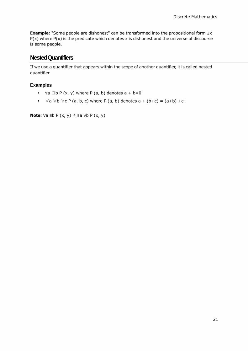
Nested Quantifiers
If we use a quantifier that appears within the scope of another quantifier, it is called nested
quantifier.
Examples
∀a ∃b P (x, y) where P (a, b) denotes a + b=0
∀a ∀b ∀c P (a, b, c) where P (a, b) denotes a + (b+c) = (a+b) +c
Note: ∀a ∃b P (x, y) ≠ ∃a ∀b P (x, y)
21
7. RULES OF INFERENCE
Discrete Mathematics
To deduce new statements from the statements whose truth that we already know, Rules of Inference are used.
What are Rules of Inference for?
Mathematical logic is often used for logical proofs. Proofs are valid arguments that
determine the truth values of mathematical statements.
An argument is a sequence of statements. The last statement is the conclusion and all its
preceding statements are called premises (or hypothesis). The symbol “∴”, (read therefore) is placed before the conclusion. A valid argument is one where the conclusion follows from the truth values of the premises.
Rules of Inference provide the templates or guidelines for constructing valid arguments
from the statements that we already have.
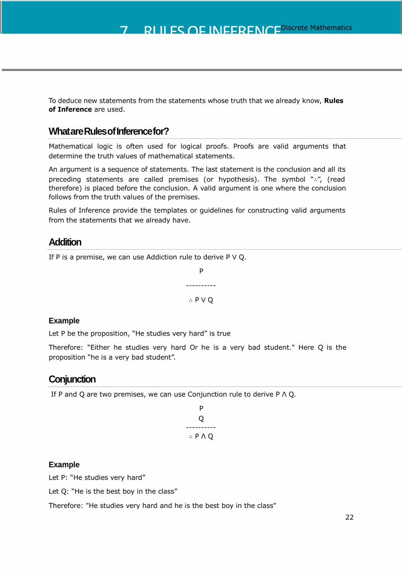
Addition
If P is a premise, we can use Addiction rule to derive P V Q.
P
----------
∴ P V Q
Example
Let P be the proposition, “He studies very hard” is true
Therefore: "Either he studies very hard Or he is a very bad student." Here Q is the
proposition “he is a very bad student”.
Conjunction
If P and Q are two premises, we can use Conjunction rule to derive P Λ Q.
P
Q ----------
∴ P Λ Q
Example
Let P: “He studies very hard”
Let Q: “He is the best boy in the class”
Therefore: "He studies very hard and he is the best boy in the class"
22

Discrete Mathematics
Simplification
If P Λ Q is a premise, we can use Simplification rule to derive P.
P Λ Q
----------
∴ P
Example
"He studies very hard and he is the best boy in the class"
Therefore: "He studies very hard"
Modus Ponens
If P and P→Q are two premises, we can use Modus Ponens to derive Q.
P→Q
P ----------
∴ Q
Example
"If you have a password, then you can log on to facebook"
"You have a password" Therefore: "You can log on to facebook"
Modus Tollens
If P→Q and ¬Q are two premises, we can use Modus Tollens to derive ¬P.
P→Q
¬Q
----------
∴ ¬P
Example
"If you have a password, then you can log on to facebook"
"You cannot log on to facebook"
Therefore: "You do not have a password "
23

Discrete Mathematics
Disjunctive Syllogism
If ¬P and P V Q are two premises, we can use Disjunctive Syllogism to derive Q.
¬P
PVQ ----------
∴ Q
Example
"The ice cream is not vanilla flavored"
"The ice cream is either vanilla flavored or chocolate flavored"
Therefore: "The ice cream is chocolate flavored”
Hypothetical Syllogism
If P → Q and Q → R are two premises, we can use Hypothetical Syllogism to derive P → R
P → Q
Q → R ----------
∴ P → R
Example
"If it rains, I shall not go to school”
"If I don't go to school, I won't need to do homework"
Therefore: "If it rains, I won't need to do homework"
Constructive Dilemma
If ( P → Q ) Λ (R → S) and P V R are two premises, we can use constructive dilemma to
derive Q V S.
( P → Q ) Λ (R → S)
PVR
---------- ∴ QVS
Example
“If it rains, I will take a leave”
“If it is hot outside, I will go for a shower”
“Either it will rain or it is hot outside”
Therefore: "I will take a leave or I will go for a shower"
24
Discrete Mathematics
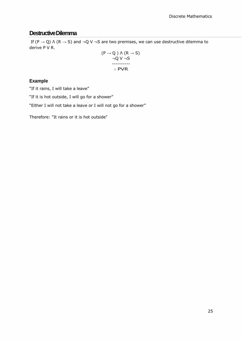
Destructive Dilemma
If (P → Q) Λ (R → S) and ¬Q V ¬S are two premises, we can use destructive dilemma to
derive P V R. (P → Q ) Λ (R → S)
¬Q V ¬S
---------- ∴ PVR
Example
“If it rains, I will take a leave”
“If it is hot outside, I will go for a shower”
“Either I will not take a leave or I will not go for a shower”
Therefore: "It rains or it is hot outside"
25

Discrete Mathematics
Part 3: Group Theory
26

8. OPERATORS AND POSTULATES
Discrete Mathematics
Group Theory is a branch of mathematics and abstract algebra that defines an algebraic structure named as group. Generally, a group comprises of a set of elements and an operation over any two elements on that set to form a third element also in that set.
In 1854, Arthur Cayley, the British Mathematician, gave the modern definition of group
for the first time:
“A set of symbols all of them different, and such that the product of any two of
them (no matter in what order), or the product of any one of them into itself, belongs to the set, is said to be a group. These symbols are not in general convertible [commutative], but are associative.”
In this chapter, we will know about operators and postulates that form the basics of set
theory, group theory and Boolean algebra.
Any set of elements in a mathematical system may be defined with a set of operators and
a number of postulates.
A binary operator defined on a set of elements is a rule that assigns to each pair of
elements a unique element from that set. For example, given the set A={1,2,3,4,5}, we
can say ⊗ is a binary operator for the operation 𝑐 = 𝑎 ⊗ 𝑏, if it specifies a rule for finding c for the pair of (a,b), such that a,b,c ∈ A.
The postulates of a mathematical system form the basic assumptions from which rules
can be deduced. The postulates are:
Closure
A set is closed with respect to a binary operator if for every pair of elements in the set,
the operator finds a unique element from that set.
Example: Let A = { 0, 1, 2, 3, 4, 5, …………. }
This set is closed under binary operator into (*), because for the operation c = a + b, for
any a, b ∈ A, the product c ∈ A.
The set is not closed under binary operator divide (÷), because, for the operation c = a +
b, for any a, b ∈ A, the product c may not be in the set A. If a = 7, b = 2, then c = 3.5.
Here a,b ∈ A but c ∉ A.
Associative Laws
A binary operator ⊗ on a set A is associative when it holds the following property:
( 𝑥 ⊗ 𝑦) ⊗ 𝑧 = 𝑥 ⊗ ( 𝑦 ⊗ 𝑧 ), where x, y, z ∈ A
Example: Let A = { 1, 2, 3, 4 }
The operator plus ( + ) is associative because for any three elements, x,y,z ∈ A, the
property (x + y) + z = x + ( y + z ) holds.
27

Discrete Mathematics
The operator minus ( - ) is not associative since
(x – y) –z ≠ x – (y – z)
Commutative Laws
A binary operator ⊗ on a set A is commutative when it holds the following property:
𝑥 ⊗ 𝑦 = 𝑦 ⊗ 𝑥, where x, y ∈ A
Example: Let A = { 1, 2, 3, 4 }
The operator plus ( + ) is commutative because for any two elements, x,y ∈ A, the
property x + y = y + x holds.
The operator minus ( - ) is not associative since
x –y ≠ y – x
Distributive Laws
Two binary operators ⊗ and ⊛ on a set A, are distributive over operator ⊛ when the
following property holds:
𝑥 ⊗ ( 𝑦 ⊛ 𝑧 ) = ( 𝑥 ⊗ 𝑦) ⊛ ( 𝑥 ⊗ 𝑧 ) , where x, y, z ∈ A
Example: Let A = { 1, 2, 3, 4 }
The operators into ( * ) and plus ( + ) are distributive over operator + because for any
three elements, x,y,z ∈ A, the property x * ( y + z ) = ( x * y ) + ( x * z ) holds.
However, these operators are not distributive over * since
x + ( y * z ) ≠ ( x + y ) * ( x + z )
Identity Element
A set A has an identity element with respect to a binary operation ⊗ on A, if there exists
an element 𝑒 ∈ A, such that the following property holds:
𝑒 ⊗ 𝑥 = 𝑥 ⊗ 𝑒, where x ∈ A
Example: Let Z = { 0, 1, 2, 3, 4, 5, ……………….. }
The element 1 is an identity element with respect to operation * since for any element
x ∈ Z,
1*x=x*1
On the other hand, there is no identity element for the operation minus ( - )
28
Discrete Mathematics
Inverse
If a set A has an identity element 𝑒 with respect to a binary operator ⊗, it is said to have
an inverse whenever for every element x ∈ A, there exists another element y ∈ A, such
that the following property holds:
𝑥 ⊗ 𝑦 = 𝑒
Example: Let A = { ………….. -4, -3, -2, -1, 0, 1, 2, 3, 4, 5, ………….. }
Given the operation plus ( + ) and 𝑒 = 0, the inverse of any element x is (-x) since x + (-
x) = 0
De Morgan’s Law
De Morgan‟s Laws gives a pair of transformations between union and intersection of two
(or more) sets in terms of their complements. The laws are:
(A⋃B)′ = A′⋂ B′
(A⋂B)′ = A′⋃ B′
Example: Let A = { 1, 2, 3, 4}, B = {1, 3, 5, 7}, and
Universal set U = { 1, 2, 3, ………, 9, 10 }
A′ = { 5, 6, 7, 8, 9, 10}
B′ = { 2, 4,6,8,9,10}
A ⋃ B = {1, 2, 3,4, 5, 7}
A⋂B = { 1,3}
(A ⋃ B)′ = { 6, 8,9,10}
A′⋂B′ = { 6, 8,9,10}
Thus, we see that (A⋃B)′ = A′⋂ B′
(A ∩ B)′ = { 2,4, 5,6,7,8,9,10}
A′ ∪ B′ = { 2,4, 5,6,7,8,9,10}
Thus, we see that (A⋂B)′ = A′⋃ B′
29

9. GROUP THEORY Discrete Mathematics
Semigroup
A finite or infinite set „S‟ with a binary operation „0‟ (Composition) is called semigroup if it
holds following two conditions simultaneously:
Closure: For every pair (a, b) ∈ S, (a 0 b) has to be present in the set S.
Associative: For every element a, b, c ∈S, (a 0 b) 0 c = a 0 (b 0 c) must hold.
Example:
The set of positive integers (excluding zero) with addition operation is a semigroup. For
example, S = {1, 2, 3,...}
Here closure property holds as for every pair (a, b) ∈ S, (a + b) is present in the set S.
For example, 1 +2 =3 ∈ S]
Associative property also holds for every element a, b, c ∈S, (a + b) + c = a + (b + c).
For example, (1 +2) +3=1+ (2+3)=5
Monoid
A monoid is a semigroup with an identity element. The identity element (denoted by e or
E) of a set S is an element such that (a 0 e) = a, for every element a ∈ S. An identity
element is also called a unit element. So, a monoid holds three properties simultaneously: Closure, Associative, Identity element.
Example
The set of positive integers (excluding zero) with multiplication operation is a monoid.
S = {1, 2, 3,...}
Here closure property holds as for every pair (a, b) ∈ S, (a × b) is present in the set S.
[For example, 1 ×2 =2 ∈ S and so on]
Associative property also holds for every element a, b, c ∈S, (a × b) × c = a × (b × c)
[For example, (1 ×2) ×3=1 × (2 ×3) =6 and so on]
Identity property also holds for every element a ∈S, (a × e) = a [For example, (2 ×1) = 2,
(3 ×1) =3 and so on]. Here identity element is 1.
Group
A group is a monoid with an inverse element. The inverse element (denoted by I) of a set
S is an element such that (a 0 I) = (I 0 a) =a, for each element a ∈ S. So, a group holds four properties simultaneously - i) Closure, ii) Associative, iii) Identity element, iv) Inverse
element. The order of a group G is the number of elements in G and the order of an
30

Discrete Mathematics
element in a group is the least positive integer n such that an is the identity element of
that group G.
Examples
The set of N×N non-singular matrices form a group under matrix multiplication operation.
The product of two N×N non-singular matrices is also an N×N non-singular matrix which
holds closure property.
Matrix multiplication itself is associative. Hence, associative property holds.
The set of N×N non-singular matrices contains the identity matrix holding the identity
element property.
As all the matrices are non-singular they all have inverse elements which are also non-
singular matrices. Hence, inverse property also holds.
Abelian Group
An abelian group G is a group for which the element pair (a,b) ∈G always holds
commutative law. So, a group holds five properties simultaneously - i) Closure, ii)
Associative, iii) Identity element, iv) Inverse element, v) Commutative.
Example
The set of positive integers (including zero) with addition operation is an abelian group.
G = {0, 1, 2, 3,…}
Here closure property holds as for every pair (a, b) ∈ S, (a + b) is present in the set S.
[For example, 1 +2 =2 ∈ S and so on]
Associative property also holds for every element a, b, c ∈S, (a + b) + c = a + (b + c)
[For example, (1 +2) +3=1 + (2 +3) =6 and so on]
Identity property also holds for every element a ∈S, (a × e) = a [For example, (2 ×1) =2,
(3 ×1) =3 and so on]. Here, identity element is 1.
Commutative property also holds for every element a ∈S, (a × b) = (b × a) [For example,
(2 ×3) = (3 ×2) =3 and so on]
Cyclic Group and Subgroup
A cyclic group is a group that can be generated by a single element. Every element of a
cyclic group is a power of some specific element which is called a generator. A cyclic group can be generated by a generator „g‟, such that every other element of the group can be written as a power of the generator „g‟.
Example
The set of complex numbers {1,-1, i, -i} under multiplication operation is a cyclic group.
There are two generators: i and –i as i1=i, i2=-1, i3=-i, i4=1 and also (–i)1=-i, (–i)2=-1,
(–i)3=i, (–i)4=1 which covers all the elements of the group. Hence, it is a cyclic group.
31

Discrete Mathematics
Note: A cyclic group is always an abelian group but not every abelian group is a cyclic
group. The rational numbers under addition is not cyclic but is abelian.
A subgroup H is a subset of a group G (denoted by H ≤ G) if it satisfies the four properties
simultaneously: Closure, Associative, Identity element, and Inverse.
A subgroup H of a group G that does not include the whole group G is called a proper
subgroup (Denoted by H<G). A subgroup of a cyclic group is cyclic and a abelian subgroup is also abelian.
Example
Let a group G = {1, i, -1, -i}
Then some subgroups are H1= {1}, H2= {1,-1},
This is not a subgroup: H3= {1, i} because that (i) -1 = -i is not in H3
Partially Ordered Set (POSET)
A partially ordered set consists of a set with a binary relation which is reflexive, anti-
symmetric and transitive. "Partially ordered set" is abbreviated as POSET.
Examples
1. The set of real numbers under binary operation less than or equal to (≤) is a poset.
Let the set S = {1, 2, 3} and the operation is ≤
The relations will be {(1, 1), (2, 2), (3, 3), (1, 2), (1, 3), (2, 3)}
This relation R is reflexive as {(1, 1), (2, 2), (3, 3)} ∈ R
This relation R is anti-symmetric, as
{(1, 2), (1, 3), (2, 3)} ∈ R and {(1, 2), (1, 3), (2, 3)} ∉ R
This relation R is also transitive. Hence, it is a poset.
2. The vertex set of a directed acyclic graph under the operation „reachability‟ is a
poset.
Hasse Diagram
The Hasse diagram of a poset is the directed graph whose vertices are the element of that
poset and the arcs covers the pairs (x, y) in the poset. If in the poset x<y, then the point
x appears lower than the point y in the Hasse diagram. If x<y<z in the poset, then the arrow is not shown between x and z as it is implicit.
Example
The poset of subsets of {1, 2, 3} = {ϕ, {1}, {2}, {3}, {1, 2}, {1, 3}, {2, 3}, {1, 2, 3}}
is shown by the following Hasse diagram:
32

Discrete Mathematics
{1, 2}
{1}
{1, 2, 3}
{1, 3} { 2}
{ϕ }
{2, 3}
{3}
Linearly Ordered Set
A Linearly ordered set or Total ordered set is a partial order set in which every pair of
element is comparable. The elements a, b ∈S are said to be comparable if either a ≤ b or
b ≤ a holds. Trichotomy law defines this total ordered set. A totally ordered set can be
defined as a distributive lattice having the property {a ∨ b, a ∧ b} = {a, b} for all values
of a and b in set S.
Example
The powerset of {a, b} ordered by ⊆ is a totally ordered set as all the elements of the
power set P= {ϕ, {a}, {b}, {a, b}} are comparable.
Example of non-total order set
A set S= {1, 2, 3, 4, 5, 6} under operation x divides y is not a total ordered set.
Here, for all (x, y) ∈S, x ≤ y have to hold but it is not true that 2 ≤ 3, as 2 does not divide
3 or 3 does not divide 2. Hence, it is not a total ordered set.
Lattice
A lattice is a poset (L, ≤) for which every pair {a, b} ∈ L has a least upper bound (denoted
by a ∨ b) and a greatest lower bound (denoted by a ∧ b).LUB ({a,b}) is called the join of
a and b.GLB ({a,b}) is called the meet of a and b.
a∨b
a b
a ∧b
33

Discrete Mathematics
Example
f
e d
c b
a
This above figure is a lattice because for every pair {a, b} ∈ L, a GLB and a LUB exists.
f
e
d
c
a b
This above figure is a not a lattice because GLB (a, b) and LUB (e, f) does not exist.
Some other lattices are discussed below:
Bounded Lattice
A lattice L becomes a bounded lattice if it has a greatest element 1 and a least element 0.
Complemented Lattice
A lattice L becomes a complemented lattice if it is a bounded lattice and if every element
in the lattice has a complement. An element x has a complement x‟ if Ǝx(x ∧x‟=0 and x ∨ x‟ = 1)
Distributive Lattice
If a lattice satisfies the following two distribute properties, it is called a distributive lattice.
a ∨ (b ∧ c) = (a ∨ b) ∧ (a ∨ c)
a ∧ (b ∨ c) = (a ∧ b) ∨ (a ∧ c)
34

Discrete Mathematics
Modular Lattice
If a lattice satisfies the following property, it is called modular lattice.
a ∧( b ∨ (a ∧ d)) = (a ∧ b) ∨ (a ∧ d)
Properties of Lattices
Idempotent Properties
ava=a
a ∧ a=a
Absorption Properties
a v (a ∧ b) = a
a ∧ (a v b) = a
Commutative Properties
avb=bva
a ∧ b=b ∧ a
Associative Properties
a v (b v c)= (a v b) v c
a ∧ (b ∧ c)= (a ∧ b) ∧ c
Dual of a Lattice
The dual of a lattice is obtained by interchanging the „v‟ and „∧’ operations.
Example
The dual of [a v (b ∧ c)] is [a ∧ (b v c)]
35

Discrete Mathematics
Part 4: Counting & Probability
36

10. COUNTING THEORY Discrete Mathematics
In daily lives, many a times one needs to find out the number of all possible outcomes for a series of events. For instance, in how many ways can a panel of judges comprising of 6 men and 4 women be chosen from among 50 men and 38 women? How many different
10 lettered PAN numbers can be generated such that the first five letters are capital
alphabets, the next four are digits and the last is again a capital letter. For solving these problems, mathematical theory of counting are used. Counting mainly encompasses fundamental counting rule, the permutation rule, and the combination rule.
The Rules of Sum and Product
The Rule of Sum and Rule of Product are used to decompose difficult counting problems
into simple problems.
The Rule of Sum: If a sequence of tasks T1, T2, …, Tm can be done in w1, w2,… wm
ways respectively (the condition is that no tasks can be performed simultaneously), then the number of ways to do one of these tasks is w1 + w2 +… +wm. If we consider two tasks A and B which are disjoint (i.e. A ∩ B = Ø), then mathematically |A ∪
B| = |A| + |B|
The Rule of Product: If a sequence of tasks T1, T2, …, Tm can be done in w1, w2,…
wm ways respectively and every task arrives after the occurrence of the previous
task, then there are w1 × w2 ×...× wm ways to perform the tasks. Mathematically, if a task B arrives after a task A, then |A×B| = |A|×|B|
Example
Question: A boy lives at X and wants to go to School at Z. From his home X he has to
first reach Y and then Y to Z. He may go X to Y by either 3 bus routes or 2 train routes. From there, he can either choose 4 bus routes or 5 train routes to reach Z. How many ways are there to go from X to Z?
Solution: From X to Y, he can go in 3+2=5 ways (Rule of Sum). Thereafter, he can go Y
to Z in 4+5 = 9 ways (Rule of Sum). Hence from X to Z he can go in 5×9 =45 ways (Rule of Product).
Permutations
A permutation is an arrangement of some elements in which order matters. In other
words a Permutation is an ordered Combination of elements.
Examples
From a set S ={x, y, z} by taking two at a time, all permutations are:
xy, yx, xz, zx, yz, zy.
37
𝑃𝑟 = 𝑛!
Discrete Mathematics
We have to form a permutation of three digit numbers from a set of numbers S=
{1, 2, 3}. Different three digit numbers will be formed when we arrange the digits. The permutation will be = 123,132,213,231,312,321
Number of Permutations
The number of permutations of „n‟ different things taken „r‟ at a time is denoted by nPr
𝑛
(𝑛 − 𝑟)!
where 𝑛! = 1.2.3. … . . (𝑛 − 1). 𝑛 Proof: Let there be „n‟ different elements.
There are n number of ways to fill up the first place. After filling the first place (n-1)
number of elements is left. Hence, there are (n-1) ways to fill up the second place. After filling the first and second place, (n-2) number of elements is left. Hence, there are (n-2) ways to fill up the third place. We can now generalize the number of ways to fill up r-th
place as [n – (r–1)] = n–r+1
So, the total no. of ways to fill up from first place upto r-th-place: nPr = n (n–1) (n–2)..... (n–r+1)
= [n(n–1)(n–2) ... (n–r+1)] [(n–r)(n–r–1)-----3.2.1] / [(n–r)(n–r–1) .. 3.2.1]
Hence,
nPr = n!/(n-r)!
Some important formulas of permutation
1. If there are n elements of which a1 are alike of some kind, a2 are alike of another
kind; a3 are alike of third kind and so on and ar are of rth kind, where (a1 + a2 + ... ar) = n. Then, number of permutations of these n objects is = n! / [ (a1!) (a2!)..... (ar!)].
2. Number of permutations of n distinct elements taking n elements at a time = nPn = n!
3. The number of permutations of n dissimilar elements taking r elements at a time,
when x particular things always occupy definite places = n-xpr-x
4. The number of permutations of n dissimilar elements when r specified things always
come together is: r! (n−r+1)!
5. The number of permutations of n dissimilar elements when r specified things never
come together is: n!–[r! (n−r+1)!]
6. The number of circular permutations of n different elements taken x elements at
time = nPx /x
7. The number of circular permutations of n different things = nPn /n
38

𝐶𝑟 = 𝑛!
Discrete Mathematics
Some Problems
Problem 1: From a bunch of 6 different cards, how many ways we can permute it?
Solution: As we are taking 6 cards at a time from a deck of 6 cards, the permutation will be
6P6 = 6! = 720
Problem 2: In how many ways can the letters of the word 'READER' be arranged?
Solution: There are 6 letters word (2 E, 1 A, 1D and 2R.) in the word 'READER'.
The permutation will be = 6! / [(2!) (1!)(1!)(2!)] = 180.
Problem 3: In how ways can the letters of the word 'ORANGE' be arranged so that the
consonants occupy only the even positions?
Solution: There are 3 vowels and 3 consonants in the word 'ORANGE'. Number of ways
of arranging the consonants among themselves= 3P3 = 3! = 6. The remaining 3 vacant
places will be filled up by 3 vowels in 3P3 = 3! = 6 ways. Hence, the total number of permutation is 6×6=36
Combinations
A combination is selection of some given elements in which order does not matter.
The number of all combinations of n things, taken r at a time is:
𝑛
𝑟! (𝑛 − 𝑟)!
Problem 1 Find the number of subsets of the set {1, 2, 3, 4, 5, 6} having 3 elements.
Solution
The cardinality of the set is 6 and we have to choose 3 elements from the set. Here, the ordering does not matter. Hence, the number of subsets will be
6C3=20.
Problem 2
There are 6 men and 5 women in a room. In how many ways we can choose 3 men and 2 women from the room?
Solution
The number of ways to choose 3 men from 6 men is 6C3 and the number of ways to choose
2 women from 5 women is 5C2
Hence, the total number of ways is: 6C3 ×5C2=20×10=200
39

𝑛−1
( 𝑘 − 1)! (𝑛 − 𝑘)! +
(𝑛
−
1)!
= (𝑛 − 1 )! (
𝑘
Discrete Mathematics
Problem 3
How many ways can you choose 3 distinct groups of 3 students from total 9 students?
Solution
Let us number the groups as 1, 2 and 3
For choosing 3 students for 1st group, the number of ways: 9C3
The number of ways for choosing 3 students for 2nd group after choosing 1st group: 6C3
The number of ways for choosing 3 students for 3rd group after choosing 1st and 2nd group: 6C3 Hence, the total number of ways =
9C3 ×6C3 × 3C3 = 84×20×1 =1680
Pascal's Identity
Pascal's identity, first derived by Blaise Pascal in 19th century, states that the number
of ways to choose k elements from n elements is equal to the summation of number of ways to choose (k-1) elements from (n-1) elements and the number of ways to choose elements from n-1 elements.
Mathematically, for any positive integers k and n: nCk = n-1Ck-1 + n-1Ck
Proof:
𝑛−1 𝐶𝑘−1 + 𝐶𝑘
= (𝑛
−
1
)!
𝑘! (𝑛 − 𝑘 − 1)!
𝑘! ( 𝑛 − 𝑘 )! +
= ( 𝑛 − 1 )! ∙ 𝑛
𝑘! (𝑛 − 𝑘)!
= 𝑛!
𝑘! ( 𝑛 − 𝑘 )!
= 𝑛𝐶𝑘
𝑛 − 𝑘
𝑘! ( 𝑛 − 𝑘 )! )
Pigeonhole Principle
In 1834, German mathematician, Peter Gustav Lejeune Dirichlet, stated a principle which
he called the drawer principle. Now, it is known as the pigeonhole principle.
Pigeonhole Principle states that if there are fewer pigeon holes than total number of
pigeons and each pigeon is put in a pigeon hole, then there must be at least one pigeon hole with more than one pigeon. If n pigeons are put into m pigeonholes where n>m, there's a hole with more than one pigeon.
Examples
1. Ten men are in a room and they are taking part in handshakes. If each person
shakes hands at least once and no man shakes the same man‟s hand more than once then two men took part in the same number of handshakes.
40
Discrete Mathematics
2. There must be at least two people in a big city with the same number of hairs on
their heads.
The Inclusion-Exclusion principle
The Inclusion-exclusion principle computes the cardinal number of the union of
multiple non-disjoint sets. For two sets A and B, the principle states:
|A ∪B| = |A| + |B| – |A∩B|
For three sets A, B and C, the principle states:
|A∪B∪C | = |A| + |B| + |C| – |A∩B| – |A∩C| – |B∩C| + |A∩B∩C |
The generalized formula:
𝑛
|⋃ 𝐴𝑖| = ∑ |𝐴𝑖 ∩ 𝐴𝑗| + ∑ |𝐴𝑖 ∩ 𝐴𝑗 ∩ 𝐴𝑘| − … … + (−1)𝑛−1|𝐴1 ∩ … ∩ 𝐴2|
𝑖=1 1≤𝑖<𝑗≤𝑛 1≤𝑖<𝑗<𝑘≤𝑛
Problem 1
How many integers from 1 to 50 are only multiples of 2 or 3?
Solution
From 1 to 100, there are 50/2=25 numbers which are multiples of 2.
There are 50/3=16 numbers which are multiples of 3.
There are 50/6=8 numbers which are multiples of both 2 and 3.
So, |A|=25, |B|=16 and |A∩B|= 8.
|A ∪ B| = |A| + |B| – |A∩B| =25 + 16 – 8 = 33
Problem 2
In a group of 50 students 24 like cold drinks and 36 like hot drinks and each student likes
at least one of the two drinks. How many like both coffee and tea?
Solution
Let X be the set of students who like cold drinks and Y be the set of people who like hot
drinks.
So, | X ∪ Y | = 50, |X| = 24, |Y| = 36
|X∩Y| = |X| + |Y| – |X∪Y| = 24 + 36 – 50 = 60 – 50 = 10
Hence, there are 10 students who like both tea and coffee.
41

11. PROBABILITY Discrete Mathematics
Closely related to the concepts of counting is Probability. We often try to guess the results of games of chance, like card games, slot machines, and lotteries; i.e. we try to find the likelihood or probability that a particular result with be obtained.
Probability can be conceptualized as finding the chance of occurrence of an event.
Mathematically, it is the study of random processes and their outcomes. The laws of probability have a wide applicability in a variety of fields like genetics, weather forecasting, opinion polls, stock markets etc.
Basic Concepts
Probability theory was invented in the 17th century by two French mathematicians, Blaise
Pascal and Pierre de Fermat, who were dealing with mathematical problems regarding of
chance.
Before proceeding to details of probability, let us get the concept of some definitions.
Random Experiment: An experiment in which all possible outcomes are known and the exact output cannot be predicted in advance is called a random experiment. Tossing a fair coin is an example of random experiment.
Sample Space: When we perform an experiment, then the set S of all possible outcomes is called the sample space. If we toss a coin, the sample space S = {H, T}
Event: Any subset of a sample space is called an event. After tossing a coin, getting Head on the top is an event.
The word "probability" means the chance of occurrence of a particular event. The best we can say is how likely they are to happen, using the idea of probability.
Probability of occurence of an event = Total
number
of
favourable
outcome
Total number of Outcomes
As the occurrence of any event varies between 0% and 100%, the probability varies
between 0 and 1.
Steps to find the probability:
Step 1: Calculate all possible outcomes of the experiment.
Step 2: Calculate the number of favorable outcomes of the experiment.
Step 3: Apply the corresponding probability formula.
42

Discrete Mathematics
Tossing a Coin
If a coin is tossed, there are two possible outcomes: Heads (H) or Tails (T)
So, Total number of outcomes = 2
Hence, the probability of getting a Head (H) on top is ½ and the probability of getting a Tails (T) on top is ½
Throwing a Dice
When a dice is thrown, six possible outcomes can be on the top: 1, 2, 3, 4, 5, 6.
The probability of any one of the numbers is 1/6
The probability of getting even numbers is 3/6=1/3
The probability of getting odd numbers is 3/6=1/3
Taking Cards From a Deck
From a deck of 52 cards, if one card is picked find the probability of an ace being drawn and also find the probability of a diamond being drawn.
Total number of possible outcomes: 52
Outcomes of being an ace: 4
Probability of being an ace = 4/52 =1/13
Probability of being a diamond = 13/52 =1/4
Probability Axioms
1. The probability of an event always varies from 0 to 1. [0 ≤ P(x) ≤ 1]
2. For an impossible event the probability is 0 and for a certain event the probability
is 1.
3. If the occurrence of one event is not influenced by another event, they are called
mutually exclusive or disjoint.
If A1, A2....An are mutually exclusive/disjoint events, then
P(Ai ∩ Aj) = ϕ for i≠j and P(A1 ∪ A2 ∪.... An) = P(A1) + P(A2)+..... P(An)
Properties of Probability
1. If there are two events x and x̅ which are complementary, then the probability of
the complementary event is:
P(x̅) = 1– P(x)
43

Discrete Mathematics
2. For two non-disjoint events A and B, the probability of the union of two events: P(A∪ B) = P(A) + P(B)
3. If an event A is a subset of another event B (i.e. A ⊂ B), then the probability of A
is less than or equal to the probability of B. Hence, A ⊂ B implies P(A) ≤ p(B)
Conditional Probability
The conditional probability of an event B is the probability that the event will occur given
an event A has already occurred. This is written as P(B|A). If event A and B are mutually
exclusive, then the conditional probability of event B after the event A will be the probability of event B that is P(B).
Mathematically: P(B|A) = P(A ∩ B) / P(A)
Problem 1
In a country 50% of all teenagers own a cycle and 30% of all teenagers own a bike and
cycle. What is the probability that a teenager owns bike given that the teenager owns a cycle?
Solution
Let us assume A is the event of teenagers owning only a cycle and B is the event of
teenagers owning only a bike.
So, P(A) = 50/100 = 0.5 and P(A ∩ B) = 30/100= 0.3 from the given problem.
P(B|A) = P(A ∩ B) / P(A) = 0.3/0.5 = 0.6
Hence, the probability that a teenager owns bike given that the teenager owns a cycle is
60%.
Problem 2
In a class, 50% of all students play cricket and 25% of all students play cricket and
volleyball. What is the probability that a student plays volleyball given that the student plays cricket?
Solution
Let us assume A is the event of students playing only cricket and B is the event of students
playing only volleyball.
So, P(A) = 50/100=0.5 and P(A ∩ B) = 25/100=0.25 from the given problem.
P(B|A) = P(A ∩ B) / P(A) =0.25/0.5 =0.5
Hence, the probability that a student plays volleyball given that the student plays cricket
is 50%.
44
Discrete Mathematics
Problem 3
Six good laptops and three defective laptops are mixed up. To find the defective laptops
all of them are tested one-by-one at random. What is the probability to find both of the defective laptops in the first two pick?
Solution
Let A be the event that we find a defective laptop in the first test and B be the event that
we find a defective laptop in the second test.
Hence, P(A ∩ B) = P(A)P(B|A) =3/9 × 2/8 = 1/21
Bayes' Theorem
Theorem: If A and B are two mutually exclusive events, where P(A) is the probability of
A and P(B) is the probability of B, P(A | B) is the probability of A given that B is true. P(B | A) is the probability of B given that A is true, then Bayes‟ Theorem states:
P(A | B) = P(B
| A)
P(A)
∑ni=1 P(B | Ai)P(Ai)
Application of Bayes’ Theorem
In situations where all the events of sample space are mutually exclusive events.
In situations where either P( Ai ∩ B ) for each Ai or P( Ai ) and P(B|Ai ) for each Ai
is known.
Problem
Consider three pen-stands. The first pen-stand contains 2 red pens and 3 blue pens; the
second one has 3 red pens and 2 blue pens; and the third one has 4 red pens and 1 blue pen. There is equal probability of each pen-stand to be selected. If one pen is drawn at random, what is the probability that it is a red pen?
Solution
Let Ai be the event that ith pen-stand is selected.
Here, i = 1,2,3. Since probability for choosing a pen-stand is equal, P(Ai) = 1/3
Let B be the event that a red pen is drawn.
The probability that a red pen is chosen among the five pens of the first pen-stand,
P(B|A1) = 2/5
The probability that a red pen is chosen among the five pens of the second pen-stand,
P(B|A2) = 3/5
The probability that a red pen is chosen among the five pens of the third pen-stand,
P(B|A3) = 4/5
45

Discrete Mathematics
According to Bayes‟ Theorem,
P(B) = P(A1).P(B|A1) + P(A2).P(B|A2) + P(A3).P(B|A3)
= 1/3 ∙ 2/5 + 1/3 ∙ 3/5 + 1/3 ∙ 4/5
= 3/5
46

Discrete Mathematics
Part 5: Mathematical Induction & Recurrence
Relations
47

12. MATHEMATICAL INDUCTION
Discrete Mathematics
Mathematical induction, is a technique for proving results or establishing statements for natural numbers. This part illustrates the method through a variety of examples.
Definition
Mathematical Induction is a mathematical technique which is used to prove a
statement, a formula or a theorem is true for every natural number.
The technique involves two steps to prove a statement, as stated below:
Step 1(Base step): It proves that a statement is true for the initial value.
Step 2(Inductive step): It proves that if the statement is true for the nth iteration (or
number n), then it is also true for (n+1)th iteration ( or number n+1).
How to Do It
Step 1: Consider an initial value for which the statement is true. It is to be shown that
the statement is true for n=initial value.
Step 2: Assume the statement is true for any value of n=k. Then prove the statement is
true for n=k+1. We actually break n=k+1 into two parts, one part is n=k (which is already proved) and try to prove the other part.
Problem 1
3n-1 is a multiple of 2 for n=1, 2, ...
Solution
Step 1: For n=1, 31-1 = 3-1 = 2 which is a multiple of 2
Step 2: Let us assume 3n-1 is true for n=k, Hence, 3k -1 is true (It is an assumption)
We have to prove that 3k+1-1 is also a multiple of 2
3k+1 – 1 = 3 × 3k – 1 = (2 × 3k) + (3k –1)
The first part (2×3k) is certain to be a multiple of 2 and the second part (3k -1) is also true
as our previous assumption.
Hence, 3k+1 – 1 is a multiple of 2.
So, it is proved that 3n – 1 is a multiple of 2.
Problem 2
1 + 3 + 5 + ... + (2n-1) = n2 for n=1, 2, ...
48

Discrete Mathematics
Solution
Step 1: For n=1, 1 = 12, Hence, step 1 is satisfied.
Step 2: Let us assume the statement is true for n=k.
Hence, 1 + 3 + 5 + ... + (2k-1) = k2 is true (It is an assumption)
We have to prove that 1 + 3 + 5 + ... + (2(k+1)-1) = (k+1)2 also holds
1 + 3 + 5 + ... + (2(k+1) – 1)
= 1 + 3 + 5 + ... + (2k+2 – 1)
= 1 + 3 + 5 + ... + (2k + 1)
= 1 + 3 + 5 + ... + (2k – 1) + (2k + 1)
= k2 + (2k + 1)
= (k + 1)2
So, 1 + 3 + 5 + ... + (2(k+1) – 1) = (k+1)2 hold which satisfies the step 2.
Hence, 1 + 3 + 5 + ... + (2n – 1) = n2 is proved.
Problem 3
Prove that (ab)n = anbn is true for every natural number n
Solution
Step 1: For n=1, (ab)1 = a1b1 = ab, Hence, step 1 is satisfied.
Step 2: Let us assume the statement is true for n=k, Hence, (ab)k = akbk is true (It is an
assumption).
We have to prove that (ab)k+1 = ak+1bk+1 also hold
Given, (ab)k = akbk
Or, (ab)k (ab)= (akbk) (ab) [Multiplying both side by „ab‟]
Or, (ab)k+1 = (aak) ( bbk)
Or, (ab)k+1 = (ak+1bk+1)
Hence, step 2 is proved.
So, (ab)n = anbn is true for every natural number n.
Strong Induction
Strong Induction is another form of mathematical induction. Through this induction
technique, we can prove that a propositional function, P(n) is true for all positive integers, n, using the following steps:
Step 1(Base step): It proves that the initial proposition P(1) true.
Step 2(Inductive step): It proves that the conditional statement
[𝑃(1) ⋀ 𝑃(2) ⋀ 𝑃(3) ⋀ … … … … ⋀ 𝑃(𝑘)] → 𝑃(𝑘 + 1) is true for positive integers k.
49
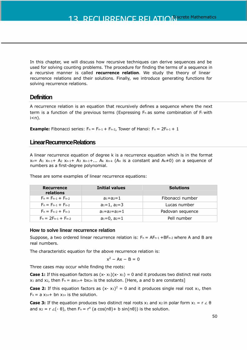
13. RECURRENCE RELATION
Discrete Mathematics
In this chapter, we will discuss how recursive techniques can derive sequences and be used for solving counting problems. The procedure for finding the terms of a sequence in a recursive manner is called recurrence relation. We study the theory of linear
recurrence relations and their solutions. Finally, we introduce generating functions for solving recurrence relations.
Definition
A recurrence relation is an equation that recursively defines a sequence where the next
term is a function of the previous terms (Expressing Fn as some combination of Fi with i<n).
Example: Fibonacci series: Fn = Fn-1 + Fn-2, Tower of Hanoi: Fn = 2Fn-1 + 1
Linear Recurrence Relations
A linear recurrence equation of degree k is a recurrence equation which is in the format xn= A1 xn-1+ A2 xn-1+ A3 xn-1+... Ak xn-k (An is a constant and Ak≠0) on a sequence of numbers as a first-degree polynomial.
These are some examples of linear recurrence equations:
How to solve linear recurrence relation
Suppose, a two ordered linear recurrence relation is: Fn = AFn-1 +BFn-2 where A and B are
real numbers.
The characteristic equation for the above recurrence relation is:
x2 − Ax − B = 0
Three cases may occur while finding the roots:
Case 1: If this equation factors as (x- x1)(x- x1) = 0 and it produces two distinct real roots
x1 and x2, then Fn = ax1n+ bx2n is the solution. [Here, a and b are constants]
Case 2: If this equation factors as (x- x1)2 = 0 and it produces single real root x1, then
Fn = a x1n+ bn x1n is the solution.
Case 3: If the equation produces two distinct real roots x1 and x2 in polar form x1 = r ∠ θ
and x2 = r ∠(- θ), then Fn = rn (a cos(nθ)+ b sin(nθ)) is the solution.
50
Recurrence relations
Initial values Solutions
Fn = Fn-1 + Fn-2 a1=a2=1 Fibonacci number
Fn = Fn-1 + Fn-2 a1=1, a2=3 Lucas number
Fn = Fn-2 + Fn-3 a1=a2=a3=1 Padovan sequence
Fn = 2Fn-1 + Fn-2 a1=0, a2=1 Pell number

Discrete Mathematics
Problem 1
Solve the recurrence relation Fn = 5Fn-1 - 6Fn-2 where F0 = 1 and F1 = 4
Solution
The characteristic equation of the recurrence relation is:
x2 – 5x + 6=0,
So, (x-3) (x-2) = 0
Hence, the roots are:
x1 = 3 and x2= 2
The roots are real and distinct. So, this is in the form of case 1
Hence, the solution is:
Fn = ax1n+ bx2n
Here, Fn = a3n+ b2n (As x1 = 3 and x2= 2)
Therefore,
1=F0 = a30+ b20 = a+b
4=F1 = a31+ b21 = 3a+2b
Solving these two equations, we get a = 2 and b = -1
Hence, the final solution is:
Fn = 2.3n + (-1) . 2n= 2.3n - 2n
Problem 2
Solve the recurrence relation Fn = 10Fn-1 - 25Fn-2 where F0 = 3 and F1 = 17
Solution
The characteristic equation of the recurrence relation is:
x2 –10x -25 =0,
So, (x – 5)2 = 0
Hence, there is single real root x1 = 5
As there is single real valued root, this is in the form of case 2
Hence, the solution is:
Fn = ax1n + bnx1n
3 = F0= a.50+ b.0.50 = a
17 = F1= a.51 + b.1.51 = 5a+5b
Solving these two equations, we get a = 3 and b = 2/5
51
Discrete Mathematics
Hence, the final solution is:
Fn = 3.5n + (2/5) .n.2n
Problem 3
Solve the recurrence relation Fn = 2Fn-1 - 2Fn-2 where F0 = 1 and F1 = 3
Solution
The characteristic equation of the recurrence relation is:
x2 –2x -2 =0
Hence, the roots are:
x1 = 1+ i and x2= 1- i
In polar form,
x1 = r ∠ θ and x2 = r ∠(- θ), where r= √2 and θ= π / 4
The roots are imaginary. So, this is in the form of case 3.
Hence, the solution is:
Fn = (√2 )n (a cos(n. π / 4) + b sin(n. π / 4))
1 = F0 = (√2 )0 (a cos(0. π / 4) + b sin(0. π / 4) ) = a
3 = F1 = (√2 )1 (a cos(1. π / 4) + b sin(1. π / 4) ) = √2 ( a/√2 + b/√2)
Solving these two equations we get a = 1 and b = 2
Hence, the final solution is:
Fn = (√2 )n (cos(n. π / 4)+ 2 sin(n. π / 4))
Particular Solutions
A recurrence relation is called non-homogeneous if it is in the form
Fn = AFn–1 + BFn-2 + F(n) where F(n) ≠ 0
The solution (an) of a non-homogeneous recurrence relation has two parts. First part is
the solution (ah) of the associated homogeneous recurrence relation and the second part is the particular solution (at). So, an= ah + at
Let F(n) = cxn and x1 and x2 are the roots of the characteristic equation:
x2 = Ax+ B which is the characteristic equation of the associated homogeneous recurrence
relation:
If x ≠ x1 and x ≠ x2, then at = Axn
If x = x1, x ≠ x2, then at = Anxn
If x= x1 = x2, then at = An2xn
52
𝐺𝑥 = 𝑎0 + 𝑎1𝑥 + 𝑎2𝑥 + … … … + 𝑎𝑘𝑥 + … … … = ∑ 𝑎𝑘𝑥𝑘
Discrete Mathematics
Problem
Solve the recurrence relation Fn = 3Fn-1 +10Fn-2 +7.5n where F0 = 4 and F1 = 3
Solution
The characteristic equation is:
x2 –3x -10 =0
Or, (x - 5)(x + 2) = 0
Or, x1= 5 and x2= -2
Since, x= x1 and x ≠ x2, the solution is:
at = Anxn = An5n
After putting the solution into the non-homogeneous relation, we get:
An5n = 3A(n – 1)5n-1 + 10A(n – 2)5n-2 + 7.5n
Dividing both sides by 5n-2, we get:
An52 = 3A(n – 1)5 + 10A(n – 2)50 + 7.52
Or, 25An = 15An – 15A + 10An – 20A + 175
Or, 35A = 175
Or, A=5
So, Fn = n5n+1
Hence, the solution is:
Fn = n5n+1 + 6.(-2)n -2.5n
Generating Functions
Generating Functions represents sequences where each term of a sequence is expressed
as a coefficient of a variable x in a formal power series.
Mathematically, for an infinite sequence, say 𝑎0, 𝑎1, 𝑎2, … … … … , 𝑎𝑘, … … …, the generating
function will be:
∞ 2 𝑘
𝑘=0
Some Areas of Application:
Generating functions can be used for the following purposes:
For solving a variety of counting problems. For example, the number of ways to make change for a Rs. 100 note with the notes of denominations Rs.1, Rs.2, Rs.5, Rs.10, Rs.20 and Rs.50
For solving recurrence relations
For proving some of the combinatorial identities For finding asymptotic formulae for terms of sequences
53

∞
∞
∞
∞
For 𝑎𝑘 = 𝐶𝑘𝑛, G(x) = ∑∞
𝑘=0 𝐶𝑘 𝑥
𝑘! = 1 + 𝑥 +
𝑥2
2! +
𝑥3
3! … … … = 𝑒𝑥
∞
Discrete Mathematics
Problem 1
What are the generating functions for the sequences {𝑎𝑘} with 𝑎𝑘 = 2 and 𝑎𝑘 = 3𝑘?
Solution
When 𝑎𝑘 = 2, generating function, G(x) = ∑𝑘=0 2𝑥𝑘 = 2 + 2𝑥 + 2𝑥
2 + 2𝑥
3 + … … …
When 𝑎𝑘 = 3𝑘, G(x) = ∑𝑘=0 3𝑘𝑥
𝑘 = 0 + 3𝑥 + 6𝑥
2 + 9𝑥
3 + … … …
Problem 2
What is the generating function of the infinite series; 1, 1, 1, 1, ……….?
Solution Here, 𝑎𝑘 = 1, 𝑓𝑜𝑟 0 ≤ 𝑘 ≤ ∞. Hence, G(x) = 1 + 𝑥 + 𝑥2 + 𝑥3 + … … … =
1
(1−𝑥)
Some Useful Generating Functions
For 𝑎𝑘 = 𝑎𝑘, G(x) = ∑𝑘=0 𝑎𝑘𝑥𝑘 = 1 + 𝑎𝑥 + 𝑎
2𝑥2 + … … … = 1⁄(1 − 𝑎𝑥)
For 𝑎𝑘 = (𝑘 + 1), G(x) = ∑𝑘=0(𝑘 + 1)𝑥
𝑘 = 1 + 2𝑥 + 3𝑥
2 + … … … =
1 (1−𝑥)2
𝑛 𝑘 = 1 + 𝐶1𝑛𝑥 + 𝐶2𝑛𝑥
2 + … … … + 𝑥2 = (1 + 𝑥)
𝑛
For 𝑎𝑘 =
1 𝑘!
, G(x) = ∑𝑘=0 𝑥𝑘
54
Discrete Mathematics
Part 6: Discrete Structures
55

14. GRAPH AND GRAPH MODELS
number of edges incident with the vertex V.
Discrete Mathematics
The previous part brought forth the different tools for reasoning, proofing and problem solving. In this part, we will study the discrete structures that form the basis of formulating many a real-life problem.
The two discrete structures that we will cover are graphs and trees. A graph is a set of
points, called nodes or vertices, which are interconnected by a set of lines called edges. The study of graphs, or graph theory is an important part of a number of disciplines in the fields of mathematics, engineering and computer science.
What is a Graph?
Definition: A graph (denoted as G = (V, E)) consists of a non-empty set of vertices or
nodes V and a set of edges E.
Example: Let us consider, a Graph is G = (V, E) where V = {a, b, c, d} and E = {{a, b},
{a, c}, {b, c},{c, d}}
a c
b d
Figure: A graph with four vertices and four edges
Even and Odd Vertex: If the degree of a vertex is even, the vertex is called an even
vertex and if the degree of a vertex is odd, the vertex is called an odd vertex.
Degree of a Vertex: The degree of a vertex V of a graph G (denoted by deg (V)) is the
Degree of a Graph: The degree of a graph is the largest vertex degree of that graph. For
the above graph the degree of the graph is 3.
The Handshaking Lemma: In a graph, the sum of all the degrees of vertices is equal to
twice the number of edges.
56
Vertex Degree Even / Odd
a 2 even b 2 even c 3 odd d 1 odd
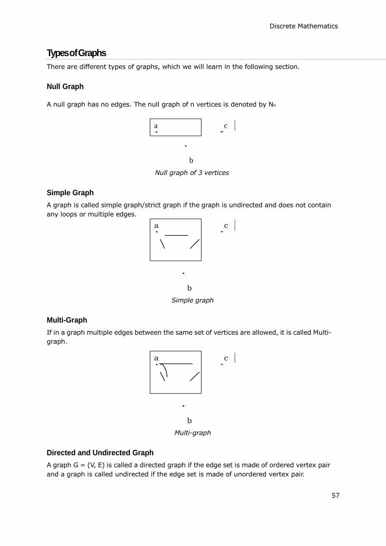
Discrete Mathematics
Types of Graphs
There are different types of graphs, which we will learn in the following section.
Null Graph
A null graph has no edges. The null graph of n vertices is denoted by Nn
a c
b
Null graph of 3 vertices
Simple Graph
A graph is called simple graph/strict graph if the graph is undirected and does not contain
any loops or multiple edges.
a c
b
Simple graph
Multi-Graph
If in a graph multiple edges between the same set of vertices are allowed, it is called Multi-
graph.
a c
b
Multi-graph
Directed and Undirected Graph
A graph G = (V, E) is called a directed graph if the edge set is made of ordered vertex pair
and a graph is called undirected if the edge set is made of unordered vertex pair.
57
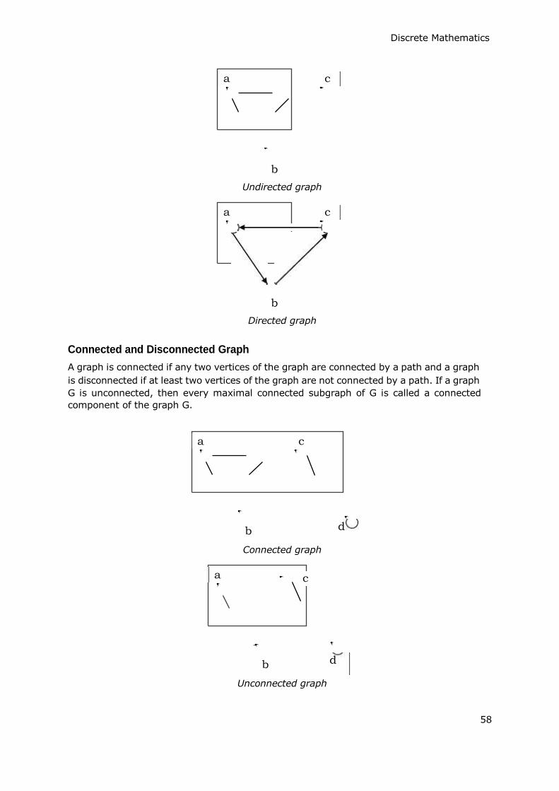
Discrete Mathematics
a c
b
Undirected graph
a c
b
Directed graph
Connected and Disconnected Graph
A graph is connected if any two vertices of the graph are connected by a path and a graph
is disconnected if at least two vertices of the graph are not connected by a path. If a graph
G is unconnected, then every maximal connected subgraph of G is called a connected component of the graph G.
a c
b
Connected graph
d
a c
b
Unconnected graph
d
58
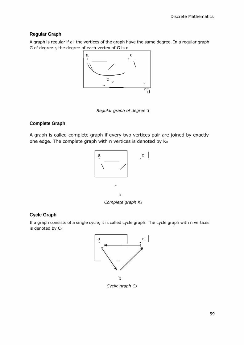
Discrete Mathematics
Regular Graph
A graph is regular if all the vertices of the graph have the same degree. In a regular graph
G of degree r, the degree of each vertex of G is r.
a c
c
d
Regular graph of degree 3
Complete Graph
A graph is called complete graph if every two vertices pair are joined by exactly
one edge. The complete graph with n vertices is denoted by Kn
a c
b
Complete graph K3
Cycle Graph
If a graph consists of a single cycle, it is called cycle graph. The cycle graph with n vertices
is denoted by Cn
a c
b
Cyclic graph C3
59

Discrete Mathematics
Bipartite Graph
If the vertex-set of a graph G can be split into two sets in such a way that each edge of
the graph joins a vertex in first set to a vertex in second set, then the graph G is called a bipartite graph. A graph G is bipartite if and only if all closed walks in G are of even length or all cycles in G are of even length.
a c
b d
Bipartite graph
Complete Bipartite Graph
A complete bipartite graph is a bipartite graph in which each vertex in the first set is joined
to every single vertex in the second set. The complete bipartite graph is denoted by Kr,s where the graph G contains x vertices in the first set and y vertices in the second set.
a c
b d
Complete bipartite graph K2,2
Representation of Graphs
There are mainly two ways to represent a graph:
Adjacency Matrix
Adjacency List
Adjacency Matrix
An Adjacency Matrix A[V][V] is a 2D array of size V×V where V is the number of vertices
in a undirected graph. If there is an edge between Vx to Vy then the value of A[Vx][ Vy]=1
and A[Vy][ Vx]=1, otherwise the value will be zero. And for a directed graph, if there is an edge between Vx to Vy, then the value of A[Vx][ Vy]=1, otherwise the value will be zero.
Adjacency Matrix of an Undirected Graph
Let us consider the following undirected graph and construct the adjacency matrix:
60

Adjacency matrix of the above undirected graph will be:
Adjacency matrix of the above directed graph will be:
Discrete Mathematics
a c
b
An undirected graph
d
Adjacency Matrix of a Directed Graph
Let us consider the following directed graph and construct its adjacency matrix:
a c
b
A directed graph
d
61
a b c d
a 0 1 1 0
b 1 0 1 0
c 1 1 0 1
d 0 0 1 0
a b c d
a 0 1 1 0
b 0 0 1 0
c 0 0 0 1
d 0 0 0 0
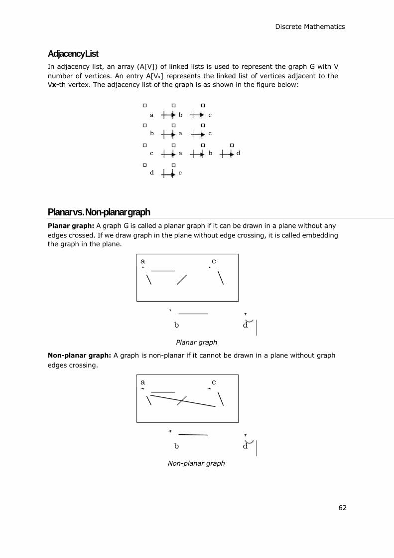
Discrete Mathematics
Adjacency List
In adjacency list, an array (A[V]) of linked lists is used to represent the graph G with V
number of vertices. An entry A[Vx] represents the linked list of vertices adjacent to the Vx-th vertex. The adjacency list of the graph is as shown in the figure below:
a
b
c
d
b
a
a
c
c
c
b d
Planar vs. Non-planar graph
Planar graph: A graph G is called a planar graph if it can be drawn in a plane without any
edges crossed. If we draw graph in the plane without edge crossing, it is called embedding the graph in the plane.
a c
b d
Planar graph
Non-planar graph: A graph is non-planar if it cannot be drawn in a plane without graph
edges crossing.
a c
b
Non-planar graph
d
62

d
Discrete Mathematics
Isomorphism
If two graphs G and H contain the same number of vertices connected in the same way,
they are called isomorphic graphs (denoted by G≅H).
It is easier to check non-isomorphism than isomorphism. If any of these following
conditions occurs, then two graphs are non-isomorphic: The number of connected components are different Vertex-set cardinalities are different Edge-set cardinalities are different Degree sequences are different
Example
The following graphs are isomorphic:
a c c a
b d b d a c b
Three isomorphic graphs
Homomorphism
A homomorphism from a graph G to a graph H is a mapping (May not be a bijective
mapping) h: GH such that: (x, y) ∈ E(G) (h(x), h(y)) ∈ E(H) . It maps adjacent vertices of graph G to the adjacent vertices of the graph H.
A homomorphism is an isomorphism if it is a bijective mapping. Homomorphism always
preserves edges and connectedness of a graph. The compositions of homomorphisms are also homomorphisms. To find out if there exists any homomorphic graph of another graph is a NP-complete problem.
Euler Graphs
A connected graph G is called an Euler graph, if there is a closed trail which includes every
edge of the graph G. An Euler path is a path that uses every edge of a graph exactly once. An Euler path starts and ends at different vertices.
An Euler circuit is a circuit that uses every edge of a graph exactly once. An Euler circuit
always starts and ends at the same vertex. A connected graph G is an Euler graph if and only if all vertices of G are of even degree, and a connected graph G is Eulerian if and only
if its edge set can be decomposed into cycles.
63

a d
Discrete Mathematics
1
7
2 3
4
f 6 c 5 e
Euler graph
The above graph is an Euler graph as “a 1 b 2 c 3 d 4 e 5 c 6 f 7 g” covers all the edges
of the graph.
a 1 b
5 4
2
d 3
Non-Euler graph
c
Hamiltonian Graphs
A connected graph G is called Hamiltonian graph if there is a cycle which includes every
vertex of G and the cycle is called Hamiltonian cycle. Hamiltonian walk in graph G is a walk that passes through each vertex exactly once.
If G is a simple graph with n vertices, where n ≥ 3 If deg(v) ≥ 1/2 n for each vertex v,
then the graph G is Hamiltonian graph. This is called Dirac's Theorem.
If G is a simple graph with n vertices, where n ≥ 2 if deg(x) + deg(y) ≥ n for each pair of
non-adjacent vertices x and y, then the graph G is Hamiltonian graph. This is called Ore's theorem.
a 1 b
5
8 6
e 4 2
d
7
3
Hamiltonian graph
c
64
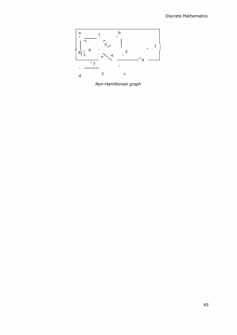
Discrete Mathematics
a 1 b
8
6
7
e
5
4 2
9
f
d 3 c
Non-Hamiltonian graph
65
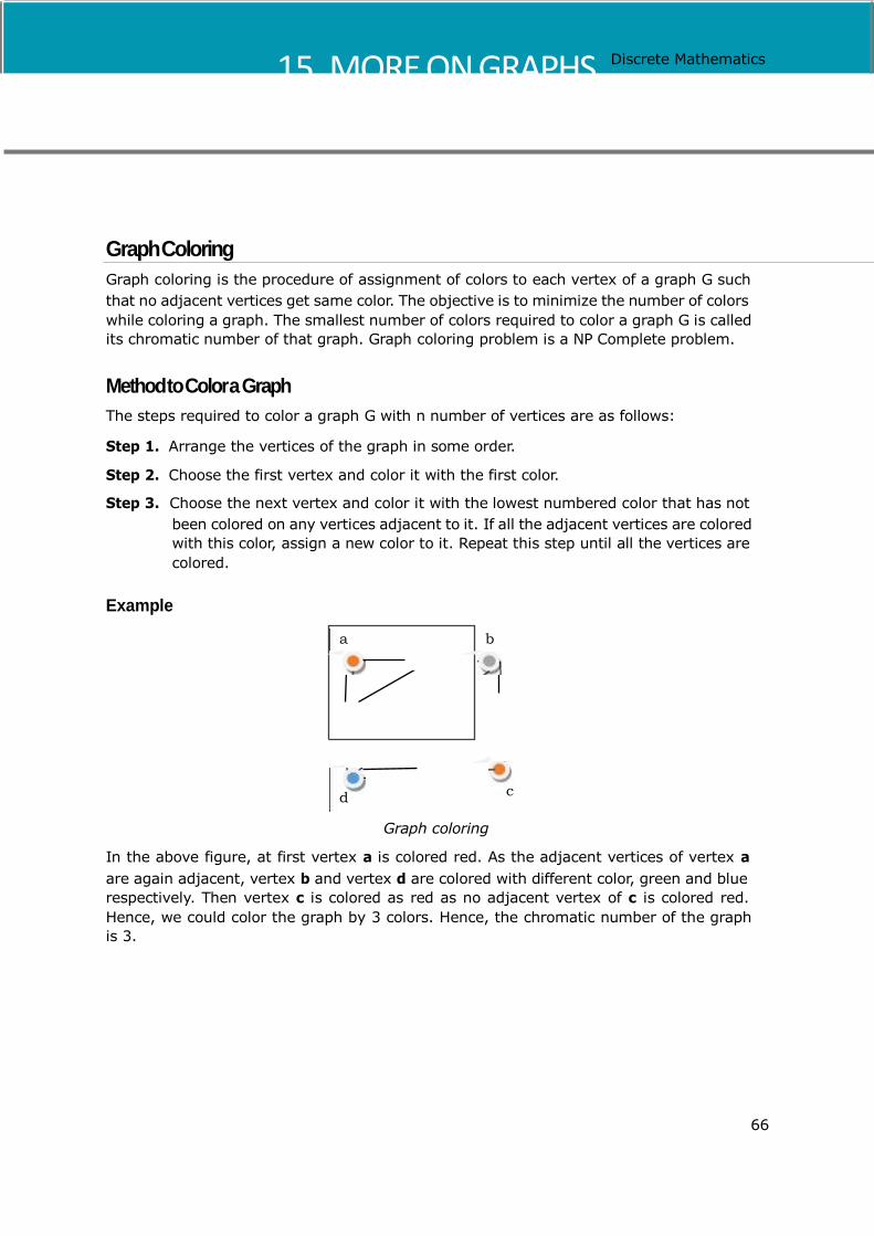
15. MORE ON GRAPHS Discrete Mathematics
Graph Coloring
Graph coloring is the procedure of assignment of colors to each vertex of a graph G such
that no adjacent vertices get same color. The objective is to minimize the number of colors
while coloring a graph. The smallest number of colors required to color a graph G is called its chromatic number of that graph. Graph coloring problem is a NP Complete problem.
Method to Color a Graph
The steps required to color a graph G with n number of vertices are as follows:
Step 1. Arrange the vertices of the graph in some order.
Step 2. Choose the first vertex and color it with the first color.
Step 3. Choose the next vertex and color it with the lowest numbered color that has not
been colored on any vertices adjacent to it. If all the adjacent vertices are colored with this color, assign a new color to it. Repeat this step until all the vertices are
colored.
Example
a b
d c
Graph coloring
In the above figure, at first vertex a is colored red. As the adjacent vertices of vertex a
are again adjacent, vertex b and vertex d are colored with different color, green and blue respectively. Then vertex c is colored as red as no adjacent vertex of c is colored red.
Hence, we could color the graph by 3 colors. Hence, the chromatic number of the graph is 3.
66
Discrete Mathematics
Applications of Graph Coloring
Some applications of graph coloring include –
Register Allocation
Map Coloring
Bipartite Graph Checking
Mobile Radio Frequency Assignment
Making time table, etc.
Graph Traversal
Graph traversal is the problem of visiting all the vertices of a graph in some systematic
order. There are mainly two ways to traverse a graph.
Breadth First Search
Depth First Search
Breadth First Search
Breadth First Search (BFS) starts at starting level-0 vertex X of the graph G. Then we visit
all the vertices that are the neighbors of X. After visiting, we mark the vertices as "visited," and place them into level-1. Then we start from the level-1 vertices and apply the same method on every level-1 vertex and so on. The BFS traversal terminates when every vertex of the graph has been visited.
BFS Algorithm:
Visit all the neighbor vertices before visiting other neighbor vertices of neighbor
vertices
Start traversing from vertex u
Visit all neighbor vertices of vertex u
Then visit all of their un-traversed neighbor vertices
Repeat until all nodes are visited
Problem
Let us take a graph (Source vertex is „a‟) and apply the BFS algorithm to find out the
traversal order.
67

Discrete Mathematics
a
1 b
5
8
d
6
e
7
3
A graph
4 2
c
Solution: Vertex „a‟ (Level-0 vertex) is traversed first and marked as “visited”. Then we will visit the adjacent vertices „b‟, „d‟ and „e‟ of vertex „a‟, marked them as level-1 and added to the “visited” list. We can traverse „b‟, „d‟ and „e‟ in any order. Next, we will visit the adjacent
vertices of „b‟ that is „c‟. Then, it is marked as level-2 and added to the “visited” list. As all vertices are travelled, the algorithm is terminated.
So the alternate orders of traversal are:
abdec
Or, abedc
Or, adbec
Or, aebdc
Or, abedc
Or,
adebc
Application of BFS
Finding the shortest path
Minimum spanning tree for un-weighted graph GPS navigation system Detecting cycles in an undirected graph Finding all nodes within one connected component
Complexity Analysis
Let G(V, E) be a graph with |V| number of vertices and |E| number of edges. If breadth
first search algorithm visits every vertex in the graph and checks every edge, then its
time complexity would be:
O(|V| + |E|). O(|E|)
It may vary between O(1) and O(|V2|)
68
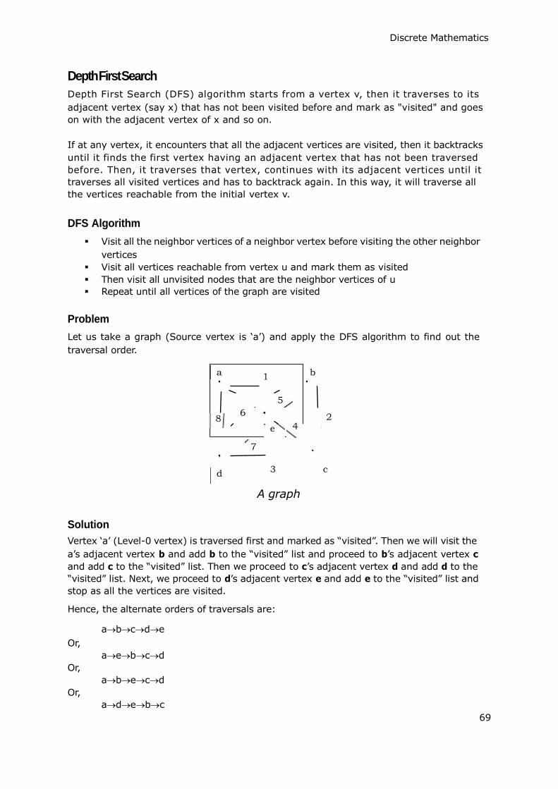
Discrete Mathematics
Depth First Search
Depth First Search (DFS) algorithm starts from a vertex v, then it traverses to its
adjacent vertex (say x) that has not been visited before and mark as "visited" and goes on with the adjacent vertex of x and so on.
If at any vertex, it encounters that all the adjacent vertices are visited, then it backtracks
until it finds the first vertex having an adjacent vertex that has not been traversed before. Then, it traverses that vertex, continues with its adjacent vertices until it traverses all visited vertices and has to backtrack again. In this way, it will traverse all the vertices reachable from the initial vertex v.
DFS Algorithm
Visit all the neighbor vertices of a neighbor vertex before visiting the other neighbor
vertices
Visit all vertices reachable from vertex u and mark them as visited
Then visit all unvisited nodes that are the neighbor vertices of u Repeat until all vertices of the graph are visited
Problem
Let us take a graph (Source vertex is „a‟) and apply the DFS algorithm to find out the
traversal order.
a 1 b
5
8 6
e 4 2
7
d 3
A graph
c
Solution
Vertex „a‟ (Level-0 vertex) is traversed first and marked as “visited”. Then we will visit the
a‟s adjacent vertex b and add b to the “visited” list and proceed to b‟s adjacent vertex c
and add c to the “visited” list. Then we proceed to c‟s adjacent vertex d and add d to the “visited” list. Next, we proceed to d‟s adjacent vertex e and add e to the “visited” list and stop as all the vertices are visited.
Hence, the alternate orders of traversals are:
abcde
Or, aebcd
Or, abecd
Or, adebc
69
Discrete Mathematics
Or,
adceb
Or, adcbe
Complexity Analysis
Let G(V, E) be a graph with |V| number of vertices and |E| number of edges. If DFS
algorithm visits every vertex in the graph and checks every edge, then the time complexity is:
Θ (|V| + |E|)
Applications
Detecting cycle in a graph
To find topological sorting
To test if a graph is bipartite
Finding connected components
Finding the bridges of a graph
Finding bi-connectivity in graphs
Solving the Knight‟s Tour problem
Solving puzzles with only one solution
70

16. INTRODUCTION TO TREES
Discrete Mathematics
Tree is a discrete structure that represents hierarchical relationships between individual elements or nodes. A tree in which a parent has no more than two children is called a binary tree.
Tree and its Properties
Definition: A Tree is a connected acyclic graph. There is a unique path between every
pair of vertices in G. A tree with N number of vertices contains (N-1) number of edges. The vertex which is of 0 degree is called root of the tree. The vertex which is of 1 degree is called leaf node of the tree and the degree of an internal node is at least 2.
Example: The following is an example of a tree:
A tree
Centers and Bi-Centers of a Tree
The center of a tree is a vertex with minimal eccentricity. The eccentricity of a vertex X in
a tree G is the maximum distance between the vertex X and any other vertex of the tree. The maximum eccentricity is the tree diameter. If a tree has only one center, it is called Central Tree and if a tree has only more than one centers, it is called Bi-central Tree. Every tree is either central or bi-central.
Algorithm to find centers and bi-centers of a tree
Step 1: Remove all the vertices of degree 1 from the given tree and also remove their
incident edges.
Step 2: Repeat step 1 until either a single vertex or two vertices joined by an edge is left.
If a single vertex is left then it is the center of the tree and if two vertices joined by an edge is left then it is the bi-center of the tree.
71

Problem 1
Find out the center/bi-center of the following tree:
f
a b c
g
Tree T1
Discrete Mathematics
d e
Solution
At first, we will remove all vertices of degree 1 and also remove their incident edges and
get the following tree:
b c d
Tree after removing vertices of degree 1 from T1
Again, we will remove all vertices of degree 1 and also remove their incident edges and get the following tree:
c
Tree after again removing vertices of degree 1
Finally we got a single vertex „c‟ and we stop the algorithm. As there is single vertex, this tree has one center „c‟ and the tree is a central tree.
72

Problem 2
Find out the center/bi-center of the following tree:
h
a b c
g
A tree T2
d e
Discrete Mathematics
f
Solution
At first, we will remove all vertices of degree 1 and also remove their incident edges and
get the following tree:
b c d e
Tree after removing vertices of degree 1 from T2
Again, we will remove all vertices of degree 1 and also remove their incident edges and get the following tree:
c d
Tree after again removing vertices of degree 1
Finally, we got two vertices „c‟ and „d‟ left, hence we stop the algorithm. As two vertices joined by an edge is left, this tree has bi-center „cd‟ and the tree is bi-central.
73
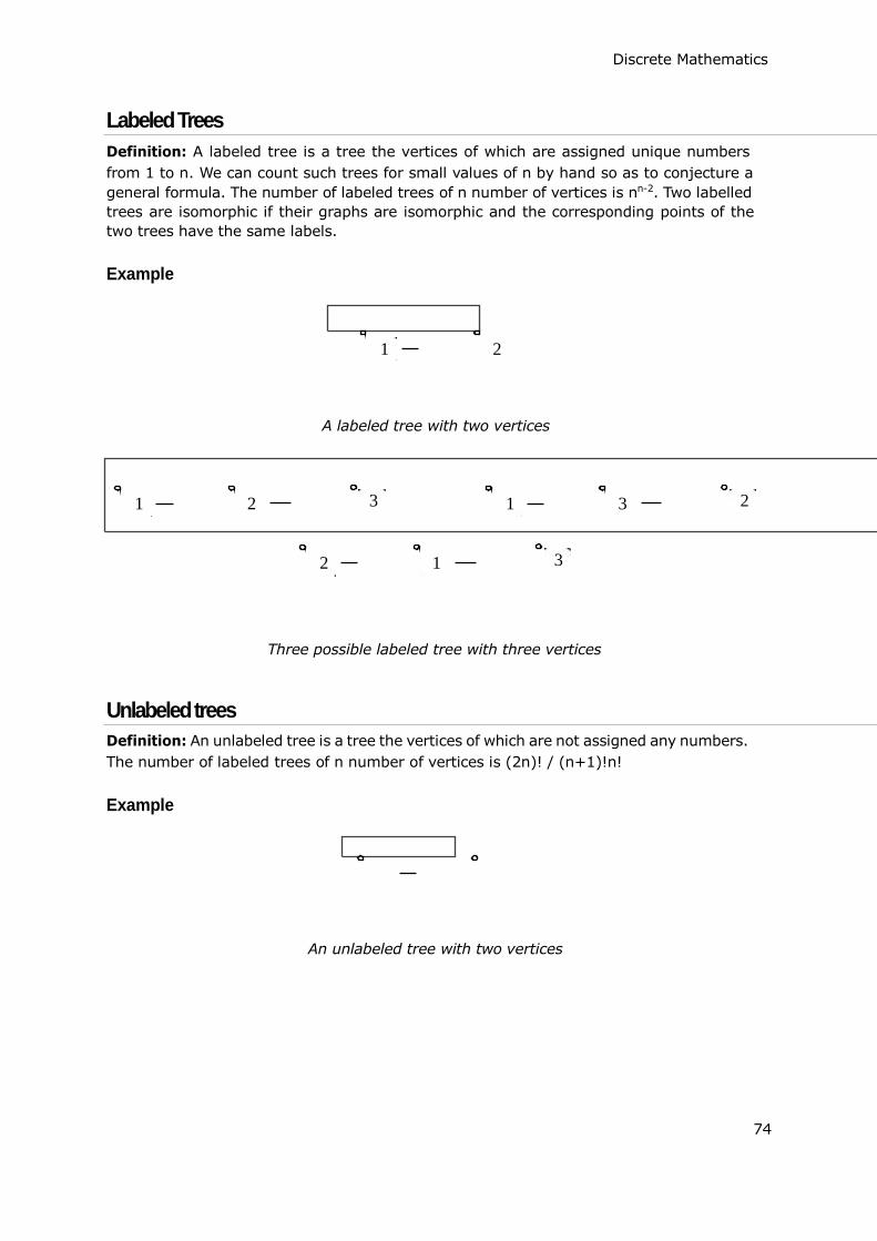
Discrete Mathematics
Labeled Trees
Definition: A labeled tree is a tree the vertices of which are assigned unique numbers
from 1 to n. We can count such trees for small values of n by hand so as to conjecture a
general formula. The number of labeled trees of n number of vertices is nn-2. Two labelled trees are isomorphic if their graphs are isomorphic and the corresponding points of the two trees have the same labels.
Example
1 2
A labeled tree with two vertices
1 2 3 1 3 2
2 1 3
Three possible labeled tree with three vertices
Unlabeled trees
Definition: An unlabeled tree is a tree the vertices of which are not assigned any numbers.
The number of labeled trees of n number of vertices is (2n)! / (n+1)!n!
Example
An unlabeled tree with two vertices
74
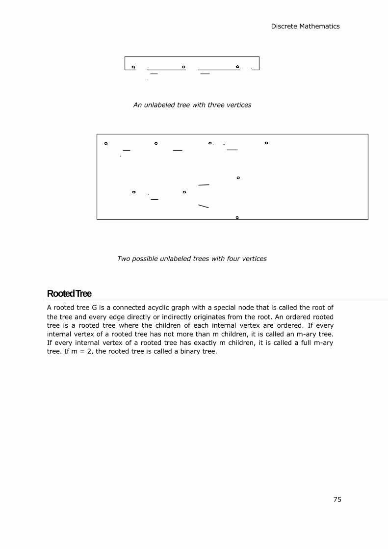
Discrete Mathematics
An unlabeled tree with three vertices
Two possible unlabeled trees with four vertices
Rooted Tree
A rooted tree G is a connected acyclic graph with a special node that is called the root of
the tree and every edge directly or indirectly originates from the root. An ordered rooted tree is a rooted tree where the children of each internal vertex are ordered. If every
internal vertex of a rooted tree has not more than m children, it is called an m-ary tree.
If every internal vertex of a rooted tree has exactly m children, it is called a full m-ary tree. If m = 2, the rooted tree is called a binary tree.
75

Root Node
Internal Node Internal
Node
Discrete Mathematics
Internal
Node
Leaf Node
Leaf Node
Leaf Node
Leaf Node
Leaf Node
Leaf Node
A Rooted Tree
Binary Search Tree
Binary Search tree is a binary tree which satisfies the following property:
X in left sub-tree of vertex V, Value(X) Value (V)
Y in right sub-tree of vertex V, Value(Y) Value (V)
So, the value of all the vertices of the left sub-tree of an internal node V are less than or
equal to V and the value of all the vertices of the right sub-tree of the internal node V are greater than or equal to V. The number of links from the root node to the deepest node is
the height of the Binary Search Tree.
Example
50
40 70
30 45 60
A Binary Search Tree
76

Complexity of Binary search tree
Discrete Mathematics
Algorithm to search for a key in BST
BST_Search(x, k)
if ( x = NIL or k = Value[x] )
return x; if ( k < Value[x])
return BST_Search (left[x], k); else
return BST_Search (right[x], k)
77
Average Case
Worst case
Space Complexity O(n) O(n) Search Complexity O(log n) O(n)
Insertion Complexity
O(log n) O(n)
Deletion Complexity
O(log n) O(n)
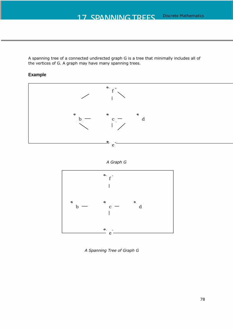
17. SPANNING TREES Discrete Mathematics
A spanning tree of a connected undirected graph G is a tree that minimally includes all of the vertices of G. A graph may have many spanning trees.
Example
f
b c
e
A Graph G
f
d
b c d
e
A Spanning Tree of Graph G
78
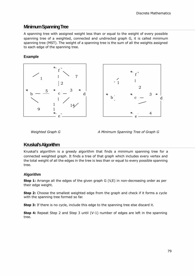
Discrete Mathematics
Minimum Spanning Tree
A spanning tree with assigned weight less than or equal to the weight of every possible
spanning tree of a weighted, connected and undirected graph G, it is called minimum
spanning tree (MST). The weight of a spanning tree is the sum of all the weights assigned to each edge of the spanning tree.
Example
b
1
5
f
c
2
3
7
d
f
1
b c
2
3
d
9
1
1
e
14
e
4
Weighted Graph G A Minimum Spanning Tree of Graph G
Kruskal's Algorithm
Kruskal's algorithm is a greedy algorithm that finds a minimum spanning tree for a
connected weighted graph. It finds a tree of that graph which includes every vertex and
the total weight of all the edges in the tree is less than or equal to every possible spanning tree.
Algorithm
Step 1: Arrange all the edges of the given graph G (V,E) in non-decreasing order as per
their edge weight. Step 2: Choose the smallest weighted edge from the graph and check if it forms a cycle with the spanning tree formed so far. Step 3: If there is no cycle, include this edge to the spanning tree else discard it. Step 4: Repeat Step 2 and Step 3 until (V-1) number of edges are left in the spanning tree.
79
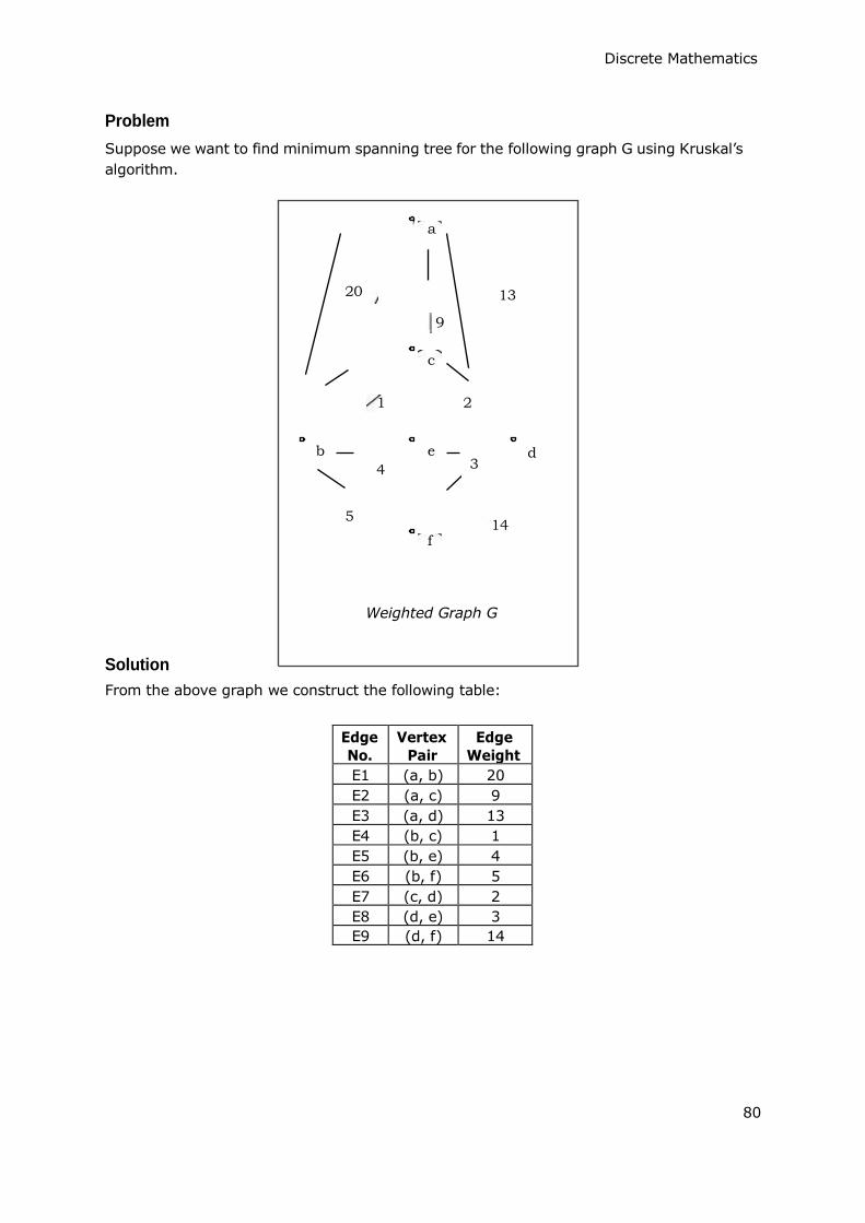
Discrete Mathematics
Problem
Suppose we want to find minimum spanning tree for the following graph G using Kruskal‟s
algorithm.
a
20 13
9
c
1
b e 4
2
3
d
5
f 14
Weighted Graph G
Solution
From the above graph we construct the following table:
80
Edge No.
Vertex Pair
Edge Weight
E1 (a, b) 20
E2 (a, c) 9
E3 (a, d) 13
E4 (b, c) 1
E5 (b, e) 4
E6 (b, f) 5
E7 (c, d) 2
E8 (d, e) 3
E9 (d, f) 14

Discrete Mathematics
Now we will rearrange the table in ascending order with respect to Edge weight:
a
a
c
1 c
b e d
b e d
f f
After adding vertices After adding edge E4
81
Edge No.
Vertex Pair
Edge Weight
E4 (b, c) 1
E7 (c, d) 2
E8 (d, e) 3
E5 (b, e) 4
E6 (b, f) 5
E2 (a, c) 9
E3 (a, d) 13
E9 (d, f) 14
E1 (a, b) 20

Discrete Mathematics
a a
1 c
2 1
c
2
b e d b e 3
d
f f
After adding edge E7 After adding edge E8
a a
9
1 c
2 1
c
2
b e 3
d b e 3
d
5 5
f f
After adding edge E6 After adding edge E2
Since we got all the 5 edges in the last figure, we stop the algorithm and this is the minimal spanning tree and its total weight is (1+2+3+5+9) = 20.
Prim's Algorithm
Prim's algorithm, discovered in 1930 by mathematicians, Vojtech Jarnik and Robert C.
Prim, is a greedy algorithm that finds a minimum spanning tree for a connected weighted
graph. It finds a tree of that graph which includes every vertex and the total weight of all the edges in the tree is less than or equal to every possible spanning tree. Prim‟s algorithm is faster on dense graphs.
82

Discrete Mathematics
Algorithm
1. Create a vertex set V that keeps track of vertices already included in MST.
2. Assign a key value to all vertices in the graph. Initialize all key values as infinite.
Assign key value as 0 for the first vertex so that it is picked first.
3. Pick a vertex „x‟ that has minimum key value and is not in V.
4. Include the vertex U to the vertex set V.
5. Update the value of all adjacent vertices of x.
6. Repeat step 3 to step 5 until the vertex set V includes all the vertices of the graph.
Problem
Suppose we want to find minimum spanning tree for the following graph G using Prim‟s
algorithm.
a
20 13
9
c
1
b e 4
2
3
d
5
f
Weighted Graph G
14
83
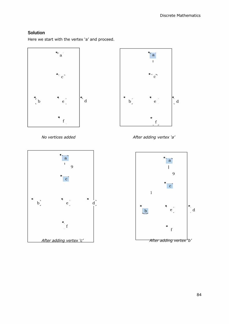
Discrete Mathematics
Solution
Here we start with the vertex „a‟ and proceed.
a
c
a
c
b e
f
d b e
f
d
No vertices added After adding vertex „a‟
a a
9
9
c
c
1
b e d
b e d
f
f
After adding vertex „c‟ After adding vertex „b‟
84

Discrete Mathematics
a a
9 9
c c 1
2 1 2
b e d b e 3
d
f f
After adding vertex „d‟ After adding vertex „e‟
a
9
c
1 2
b e
5
3 d
f
After adding vertex „f‟
This is the minimal spanning tree and its total weight is (1+2+3+5+9) = 20.
85

Discrete Mathematics
Part 7: Boolean Algebra
86
18. BOOLEAN EXPRESSIONS AND FUNCTIONS
Discrete Mathematics
Boolean algebra is algebra of logic. It deals with variables that can have two discrete values, 0 (False) and 1 (True); and operations that have logical significance. The earliest method of manipulating symbolic logic was invented by George Boole and subsequently came to be known as Boolean Algebra.
Boolean algebra has now become an indispensable tool in computer science for its wide
applicability in switching theory, building basic electronic circuits and design of digital computers.
Boolean Functions
A Boolean function is a special kind of mathematical function f: Xn → X of degree n,
where X = {0, 1} is a Boolean domain and n is a non-negative integer. It describes the
way how to derive Boolean output from Boolean inputs.
Example: Let, F(A, B) = A‟B‟. This is a function of degree 2 from the set of ordered pairs
of Boolean variables to the set {0, 1} where F(0, 0) = 1, F(0, 1) = 0, F(1, 0) = 0 and F(1, 1) = 0
Boolean Expressions
A Boolean expression always produces a Boolean value. A Boolean expression is
composed of a combination of the Boolean constants (True or False), Boolean variables and logical connectives. Each Boolean expression represents a Boolean function.
Example: AB‟C is a Boolean expression.
Boolean Identities
Double Complement Law
~(~A) = A
Complement Law
A + ~A = 1 (OR Form)
A · ~A = 0 (AND Form)
Idempotent Law
A+A=A (OR Form)
A·A=A (AND Form)
Identity Law
A+0=A (OR Form)
A·1=A (AND Form)
87

Discrete Mathematics
Dominance Law
A+1=1 (OR Form)
A·0=0 (AND Form)
Commutative Law
A+B=B+A (OR Form)
A· B = B · A (AND Form)
Associative Law
A + (B + C) = (A + B) + C (OR Form)
A· (B · C) = (A · B) · C (AND Form)
Absorption Law
A· (A + B) = A
A + (A · B) = A
Simplification Law
A · (~A + B) = A · B
A + (~A · B) = A + B A · B + A · C + ~B · C = A · B + ~B ·C
Distributive Law
A + (B · C) = (A + B) · (A + C)
A · (B + C) = (A · B) + (A · C)
De-Morgan's Law
~(A · B) = ~A + ~B ~(A+ B) = ~A · ~B
Canonical Forms
For a Boolean expression there are two kinds of canonical forms:
1. The sum of minterms (SOM) form
2. The product of maxterms (POM) form
The Sum of Minterms (SOM) or Sum of Products (SOP) form
A minterm is a product of all variables taken either in their direct or complemented form.
Any Boolean function can be expressed as a sum of its 1-minterms and the inverse of the
function can be expressed as a sum of its 0-minterms. Hence,
F (list of variables) = Σ (list of 1-minterm indices)
and
F‟ (list of variables) = Σ (list of 0-minterm indices)
88
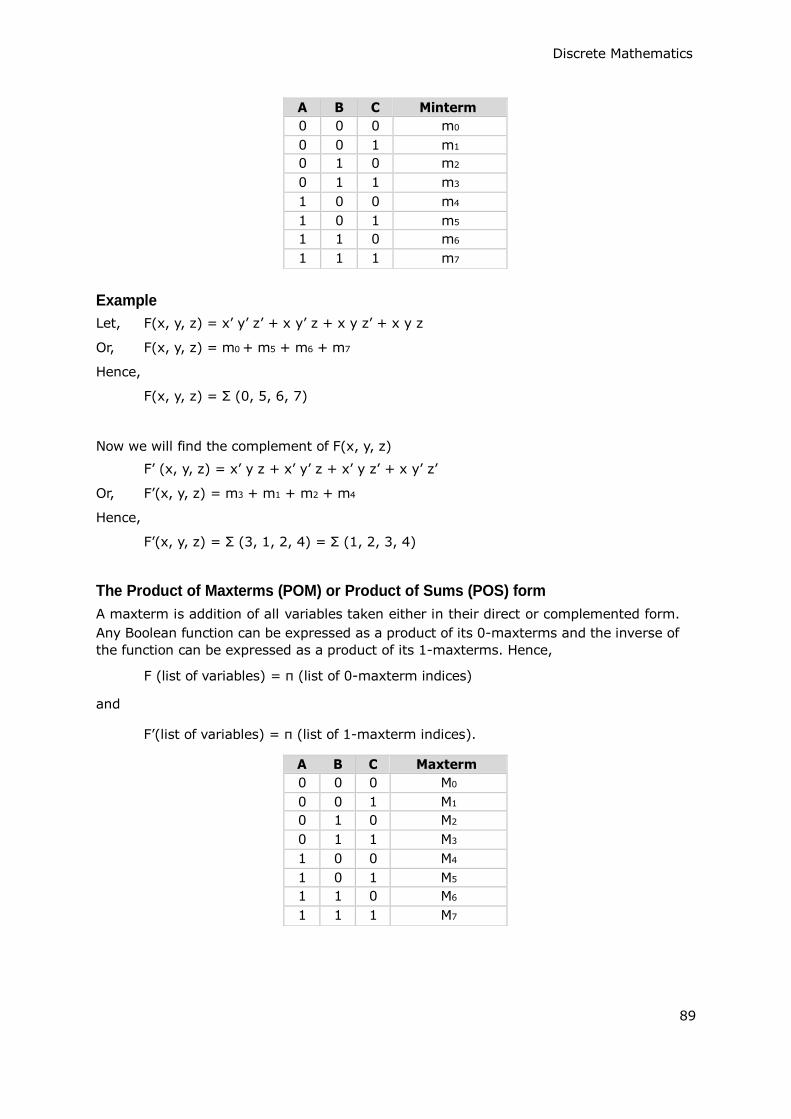
F‟(list of variables) = π (list of 1-maxterm indices).
Discrete Mathematics
Example
Let, F(x, y, z) = x‟ y‟ z‟ + x y‟ z + x y z‟ + x y z
Or, F(x, y, z) = m0 + m5 + m6 + m7
Hence,
F(x, y, z) = Σ (0, 5, 6, 7)
Now we will find the complement of F(x, y, z)
F‟ (x, y, z) = x‟ y z + x‟ y‟ z + x‟ y z‟ + x y‟ z‟
Or, F‟(x, y, z) = m3 + m1 + m2 + m4
Hence,
F‟(x, y, z) = Σ (3, 1, 2, 4) = Σ (1, 2, 3, 4)
The Product of Maxterms (POM) or Product of Sums (POS) form
A maxterm is addition of all variables taken either in their direct or complemented form.
Any Boolean function can be expressed as a product of its 0-maxterms and the inverse of the function can be expressed as a product of its 1-maxterms. Hence,
F (list of variables) = π (list of 0-maxterm indices)
and
89
A B C Maxterm
0 0 0 M0
0 0 1 M1
0 1 0 M2
0 1 1 M3
1 0 0 M4
1 0 1 M5
1 1 0 M6
1 1 1 M7
A B C Minterm
0 0 0 m0
0 0 1 m1
0 1 0 m2
0 1 1 m3
1 0 0 m4
1 0 1 m5
1 1 0 m6
1 1 1 m7

Truth table of NOT Gate
it gives low output. A dot (.) is used to show the AND operation.
Truth table of AND Gate
Discrete Mathematics
Example
Let, F(x, y, z) = (x+y+z) • (x+y+z‟) • (x+y‟+z) • (x‟+y+z)
Or, F(x, y, z) = M0 • M1 • M2 • M4
Hence,
F (x, y, z) = Π(0, 1, 2, 4)
F‟'(x, y, z) = (x+y‟+z‟) • (x‟+y+z‟) • (x‟+y‟+z) • (x‟+y‟+z‟)
Or, F(x, y, z) = M3 • M5 • M6 • M7
Hence,
F ' (x, y, z) = Π(3, 5, 6, 7)
Logic Gates
Boolean functions are implemented by using logic gates. The following are the logic gates:
NOT Gate
A NOT gate inverts a single bit input to a single bit of output.
AND Gate
An AND gate is a logic gate that gives a high output only if all its inputs are high, otherwise
OR Gate
An OR gate is a logic gate that gives high output if at least one of the inputs is high. A plus
(+) is used to show the OR operation.
90
A B A.B
0 0 0
0 1 0
1 0 0
1 1 1
A ~A
0 1
1 0

Truth table of OR Gate
Truth table of NAND Gate
Truth table of NOR Gate
Truth table of XOR Gate
Discrete Mathematics
NAND Gate
A NAND gate is a logic gate that gives a low output only if all its inputs are high, otherwise
it gives high output.
NOR Gate
An NOR gate is a logic gate that gives high output if both the inputs are low, otherwise it
gives low output.
XOR (Exclusive OR) Gate
An XOR gate is a logic gate that gives high output if the inputs are different, otherwise it
gives low output.
91
A B A⊕B
0 0 0
0 1 1
1 0 1
1 1 0
A B A+B
0 0 0
0 1 1
1 0 1
1 1 1
A B ~ (A.B)
0 0 1
0 1 1
1 0 1
1 1 0
A B ~ (A+B)
0 0 1
0 1 0
1 0 0
1 1 0

Truth table of X-NOR Gate
Discrete Mathematics
X-NOR (Exclusive NOR) Gate
An EX-NOR gate is a logic gate that gives high output if the inputs are same, otherwise it
gives low output.
92
A B A X-NOR B
0 0 1
0 1 0
1 0 0
1 1 1
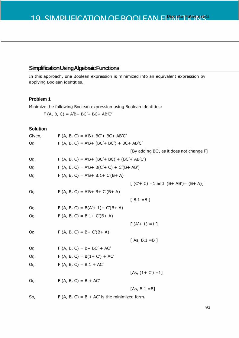
19. SIMPLIFICATION OF BOOLEAN FUNCTIONS
Discrete Mathematics
Simplification Using Algebraic Functions
In this approach, one Boolean expression is minimized into an equivalent expression by
applying Boolean identities.
Problem 1
Minimize the following Boolean expression using Boolean identities:
F (A, B, C) = A‟B+ BC‟+ BC+ AB‟C‟
Solution
Given, F (A, B, C) = A‟B+ BC‟+ BC+ AB‟C‟
Or, F (A, B, C) = A‟B+ (BC‟+ BC‟) + BC+ AB‟C‟
[By adding BC‟, as it does not change F]
Or, F (A, B, C) = A‟B+ (BC‟+ BC) + (BC‟+ AB‟C‟)
Or, F (A, B, C) = A‟B+ B(C‟+ C) + C‟(B+ AB‟)
Or, F (A, B, C) = A‟B+ B.1+ C‟(B+ A)
[ (C‟+ C) =1 and (B+ AB‟)= (B+ A)]
Or, F (A, B, C) = A‟B+ B+ C‟(B+ A)
[ B.1 =B ]
Or, F (A, B, C) = B(A‟+ 1)+ C‟(B+ A)
Or, F (A, B, C) = B.1+ C‟(B+ A)
[ (A‟+ 1) =1 ]
Or, F (A, B, C) = B+ C‟(B+ A)
[ As, B.1 =B ]
Or, F (A, B, C) = B+ BC‟ + AC‟
Or, F (A, B, C) = B(1+ C‟) + AC‟
Or, F (A, B, C) = B.1 + AC‟
[As, (1+ C‟) =1]
Or, F (A, B, C) = B + AC‟
[As, B.1 =B]
So, F (A, B, C) = B + AC‟ is the minimized form.
93

An arbitrary truth table is taken below:
Truth table
Discrete Mathematics
Problem 2
Minimize the following Boolean expression using Boolean identities:
F (A, B, C) = (A+B) (B+ C)
Solution
Given, F (A, B, C) = (A+B) (A+ C)
Or, F (A, B, C) = A.A+A.C+B.A+ B.C [Applying distributive Rule]
Or, F (A, B, C) = A+A.C+B.A+ B.C [Applying Idempotent Law]
Or, F (A, B, C) = A(1+C)+B.A+ B.C [Applying distributive Law]
Or, F (A, B, C) = A+B.A+ B.C [Applying dominance Law]
Or, F (A, B, C) = (A+1).A+ B.C [Applying distributive Law]
Or, F (A, B, C) = 1.A+ B.C [Applying dominance Law]
Or, F (A, B, C) = A+ B.C [Applying dominance Law]
So, F (A, B, C) = A+ BC is the minimized form.
Karnaugh Maps
The Karnaugh map (K–map), introduced by Maurice Karnaughin in 1953, is a grid-like
representation of a truth table which is used to simplify boolean algebra expressions. A
Karnaugh map has zero and one entries at different positions. It provides grouping together Boolean expressions with common factors and eliminates unwanted variables
from the expression. In a K-map, crossing a vertical or horizontal cell boundary is always a change of only one variable.
Example 1
Now we will make a k-map for the above truth table:
94
A B AoperationB
0 0 w
0 1 x
1 0 y
1 1 z
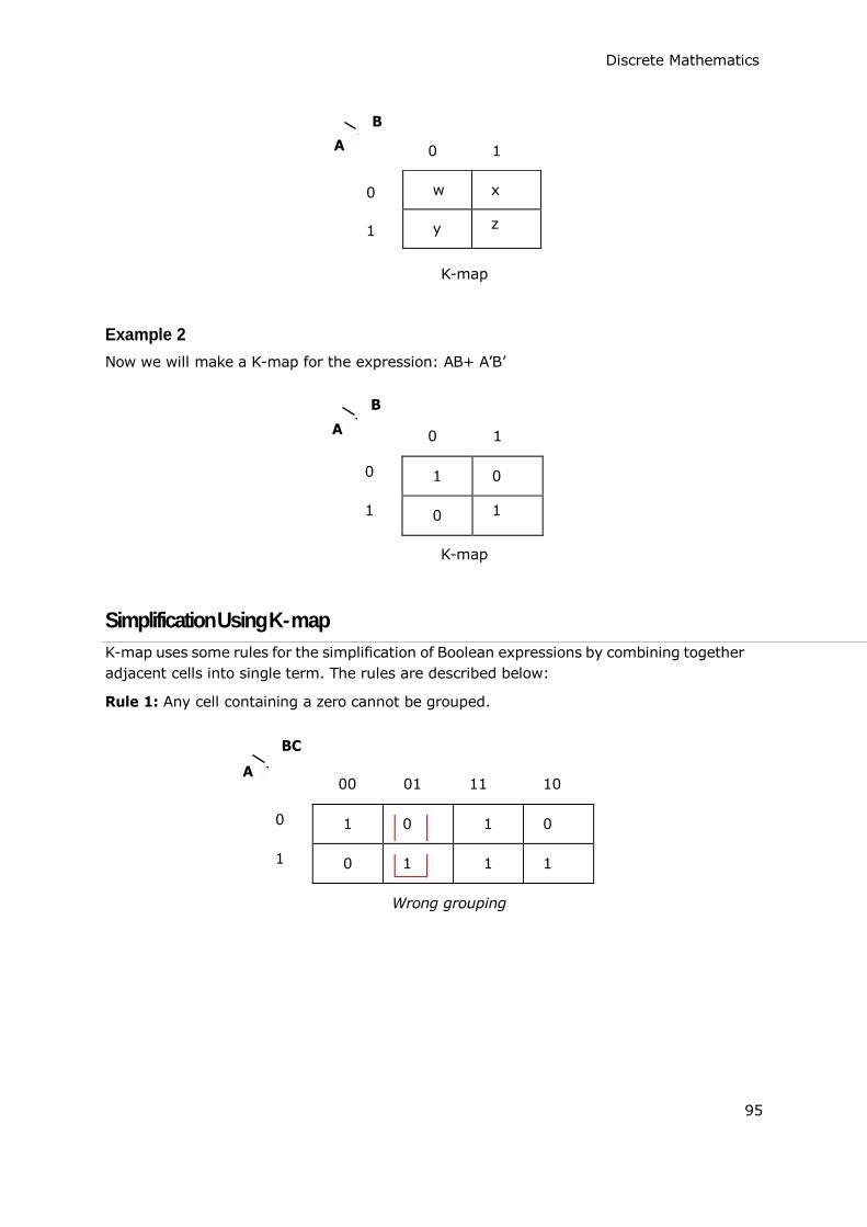
0 1
0 1
00 01 11 10
Wrong grouping
Discrete Mathematics
B
A
0
1
K-map
Example 2
Now we will make a K-map for the expression: AB+ A‟B‟
B
A
0
1
K-map
Simplification Using K- map
K-map uses some rules for the simplification of Boolean expressions by combining together
adjacent cells into single term. The rules are described below:
Rule 1: Any cell containing a zero cannot be grouped.
BC
A
0
1
95
1 0 1 0
0 1 1 1
1 0
0 1
w x
y z

00 01 11 10
Wrong grouping
00 01 11 10
Wrong diagonal grouping
00 01 11 10
Proper vertical grouping
00 01 11 10
Proper horizontal grouping
Discrete Mathematics
Rule 2: Groups must contain 2n cells (n starting from 1).
BC
A
0
1
Rule 3: Grouping must be horizontal or vertical, but must not be diagonal.
BC
A
0
1
BC
A
0
1
BC
A
0
1
96
1 1 1 0
0 0 1 1
1 1 1 0
0 0 1 1
1 0 1 0
0 1 1 1
1 1 1 0
0 0 1 1
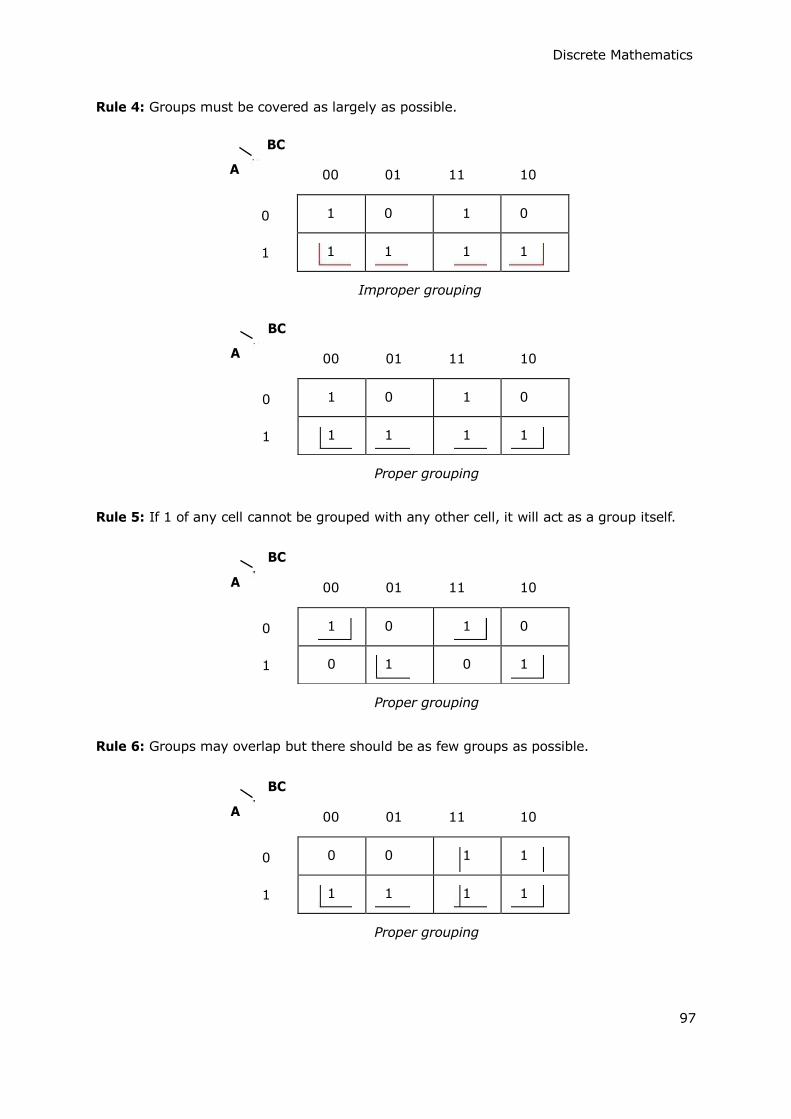
00 01 11 10
Improper grouping
00 01 11 10
Proper grouping
00 01 11 10
Proper grouping
00 01 11 10
Proper grouping
Discrete Mathematics
Rule 4: Groups must be covered as largely as possible.
BC
A
0
1
BC
A
0
1
Rule 5: If 1 of any cell cannot be grouped with any other cell, it will act as a group itself.
BC
A
0
1
Rule 6: Groups may overlap but there should be as few groups as possible.
BC
A
0
1
97
1 0 1 0
1 1 1 1
1 0 1 0
0 1 0 1
0 0 1 1
1 1 1 1
1 0 1 0
1 1 1 1
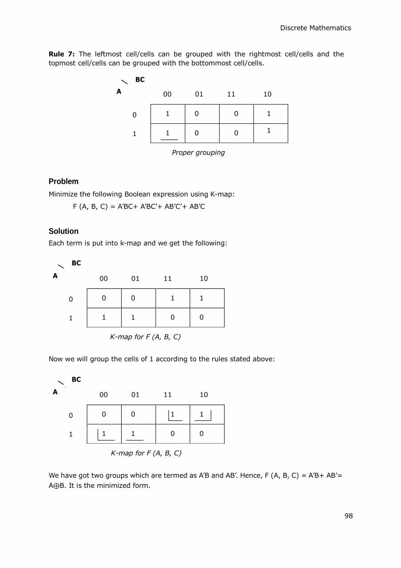
00 01 11 10
Proper grouping
00 01 11 10
K-map for F (A, B, C)
00 01 11 10
K-map for F (A, B, C)
Discrete Mathematics
Rule 7: The leftmost cell/cells can be grouped with the rightmost cell/cells and the
topmost cell/cells can be grouped with the bottommost cell/cells.
BC
A
0
1
Problem
Minimize the following Boolean expression using K-map:
F (A, B, C) = A‟BC+ A‟BC‟+ AB‟C‟+ AB‟C
Solution
Each term is put into k-map and we get the following:
BC
A
0
1
Now we will group the cells of 1 according to the rules stated above:
BC
A
0
1
We have got two groups which are termed as A‟B and AB‟. Hence, F (A, B, C) = A‟B+ AB‟=
A⊕B. It is the minimized form.
98
0 0 1 1
1 1 0 0
0 0 1 1
1 1 0 0
1 0 0 1
1 0 0 1


