Embed Size (px)
Citation preview

Discrete Event Simulation of Mobility and Spatio-TemporalSpectrum Demand
Shridhar Chandan
Thesis submitted to the Faculty of the
Virginia Polytechnic Institute and State University
in partial fulfillment of the requirements for the degree of
Master of Science
in
Computer Science & Applications
Anil Vullikanti, Chair
Madhav Marathe
Achla Marathe
Dec 9, 2013
Blacksburg, Virginia
Keywords: Wireless Communication Networks, Spectrum Demand, Discrete Event
Simulation
Copyright 2013, Shridhar Chandan

Discrete Event Simulation of Mobility and Spatio-Temporal Spectrum
Demand
Shridhar Chandan
(ABSTRACT)
Realistic mobility and cellular traffic modeling are key to various wireless networking ap-
plications and have a significant impact on network performance. Planning and designing,
network resource allocation and performance evaluation in cellular networks require realistic
traffic modeling. We propose a Discrete Event Simulation framework, Diamond - (Dis-
crete Event Simulation of Mobility and Spatio-Temporal Spectrum Demand) to model and
analyze realistic activity based mobility and spectrum demand patterns. The framework
can be used for spatio-temporal estimation of load, in deciding the location of a new base
station, contingency planning, and estimating the resilience of the existing infrastructure.
The novelty of this framework lies in its ability to capture a variety of complex, realistic and
dynamically changing events effectively. Our initial results show that the framework can be
instrumental in contingency planning and dynamic spectrum allocation.

Acknowledgments
I am greatly indebted to my advisor, Dr. Anil Vullikanti for his continued support, pa-
tience and encouragement. This thesis would not have completed without his philosophical
insights and immense knowledge. I would also like to thank Dr. Madhav Marathe and Dr.
Achla Marathe for their innovative ideas and feedback. I would also thank Sudip Saha and
Sudarshan Aji for formal and informal discussions related to the topics of this thesis, peer
reviewing the code and actively participating in various aspects of this thesis. Working in
the NDSSL lab was certainly a most wonderful and memorable journey.
Most importantly i would like to thank my family and friends who have always been there
for me and supported me.
iii

Contents
1 Introduction 1
1.1 Proposed Solution . . . . . . . . . . . . . . . . . . . . . . . . . . . . . . . . . 2
1.2 Thesis Organization . . . . . . . . . . . . . . . . . . . . . . . . . . . . . . . . 3
2 Background 4
2.1 Discrete Event Simulation Fundamentals . . . . . . . . . . . . . . . . . . . . 4
2.1.1 Time . . . . . . . . . . . . . . . . . . . . . . . . . . . . . . . . . . . . 5
2.1.2 Event-Driven Execution . . . . . . . . . . . . . . . . . . . . . . . . . 5
2.1.3 Discrete Event Simulation Program . . . . . . . . . . . . . . . . . . . 6
2.1.4 Starting and Stopping the Simulation . . . . . . . . . . . . . . . . . . 8
2.2 Nearest Neighbor Search . . . . . . . . . . . . . . . . . . . . . . . . . . . . . 9
3 Related Work 10
3.1 Dynamic Modeling Environment for Socio-communication Networks (Dymen-
son) . . . . . . . . . . . . . . . . . . . . . . . . . . . . . . . . . . . . . . . . 10
3.2 Disaster Management Studies . . . . . . . . . . . . . . . . . . . . . . . . . . 12
3.3 Pleiades . . . . . . . . . . . . . . . . . . . . . . . . . . . . . . . . . . . . . . 13
3.4 The IDES Framework . . . . . . . . . . . . . . . . . . . . . . . . . . . . . . . 14
iv

3.5 FastTrans . . . . . . . . . . . . . . . . . . . . . . . . . . . . . . . . . . . . . 14
4 System Design and Implementation 15
4.1 Proposed System . . . . . . . . . . . . . . . . . . . . . . . . . . . . . . . . . 15
4.2 Input, Configuration, and Output . . . . . . . . . . . . . . . . . . . . . . . . 17
4.2.1 Modeling Input . . . . . . . . . . . . . . . . . . . . . . . . . . . . . . 18
4.2.2 Configuration . . . . . . . . . . . . . . . . . . . . . . . . . . . . . . . 24
4.2.3 Output . . . . . . . . . . . . . . . . . . . . . . . . . . . . . . . . . . . 25
4.3 Implementation Details . . . . . . . . . . . . . . . . . . . . . . . . . . . . . . 26
4.3.1 Assumptions . . . . . . . . . . . . . . . . . . . . . . . . . . . . . . . . 26
4.3.2 System Invariants . . . . . . . . . . . . . . . . . . . . . . . . . . . . . 27
4.3.3 Algorithmic Description of Events and their Corresponding Actions . 27
4.3.4 Optimizations . . . . . . . . . . . . . . . . . . . . . . . . . . . . . . . 32
5 Evaluation 36
5.1 Hypothetical Study . . . . . . . . . . . . . . . . . . . . . . . . . . . . . . . . 36
5.2 Results . . . . . . . . . . . . . . . . . . . . . . . . . . . . . . . . . . . . . . . 36
5.3 Comparison with Dymenson [15, 12] . . . . . . . . . . . . . . . . . . . . . . 45
5.4 Comparison with NPS-1 Study [8] . . . . . . . . . . . . . . . . . . . . . . . . 48
6 Conclusion and Future Work 50
6.1 Future Work . . . . . . . . . . . . . . . . . . . . . . . . . . . . . . . . . . . . 50
Bibliography 52
v

List of Figures
2.1 Data structures in a discrete-event simulation program . . . . . . . . . . . . 6
2.2 Two Major Components of Simulation . . . . . . . . . . . . . . . . . . . . . 7
3.1 The overall architecture of Dymenson. The rounded boxes represent modules
of Dymenson and the rectangles represent input datasets. . . . . . . . . . . . 11
3.2 User Call Behavior Modeled in [8, 22] . . . . . . . . . . . . . . . . . . . . . 12
4.1 Flow Diagram of the DES . . . . . . . . . . . . . . . . . . . . . . . . . . . . 17
4.2 Event Queue . . . . . . . . . . . . . . . . . . . . . . . . . . . . . . . . . . . 17
4.3 Event Dependency Diaram . . . . . . . . . . . . . . . . . . . . . . . . . . . . 28
4.4 Mobility Optimization: Example Scenario . . . . . . . . . . . . . . . . . . . . 32
5.1 Service Range vs. No. of Successfull Calls . . . . . . . . . . . . . . . . . . . 38
5.2 Capacity vs. No. of Successfull Calls . . . . . . . . . . . . . . . . . . . . . . 39
5.3 Cell Tower down % vs. No. of Successfull Calls . . . . . . . . . . . . . . . . 40
5.4 Time (in min) vs. No. of Successfull Calls . . . . . . . . . . . . . . . . . . . 42
5.5 Cell Tower Up % vs. No. of Successfull Calls . . . . . . . . . . . . . . . . . 43
5.6 Time (in min) vs. No. of Successfull Calls . . . . . . . . . . . . . . . . . . . 44
5.7 EBR % vs. EBR Receivers . . . . . . . . . . . . . . . . . . . . . . . . . . . . 45
vi
5.8 Cell Tower Up % vs. EBR receievrs . . . . . . . . . . . . . . . . . . . . . . . 47
5.9 No of Calls Simulated vs. Time taken in sec . . . . . . . . . . . . . . . . . . 48
vii

List of Tables
4.1 Supported Event Types . . . . . . . . . . . . . . . . . . . . . . . . . . . . . . 16
5.1 Varying Service Range . . . . . . . . . . . . . . . . . . . . . . . . . . . . . . 37
5.2 Varying Capacity . . . . . . . . . . . . . . . . . . . . . . . . . . . . . . . . . 38
5.3 Varying Cell Tower Down % . . . . . . . . . . . . . . . . . . . . . . . . . . . 39
5.4 Varying Cell Tower Down % Time Series Analysis . . . . . . . . . . . . . . 41
5.5 Varying Cell Tower Up % . . . . . . . . . . . . . . . . . . . . . . . . . . . . 41
5.6 Varying Cell Tower Up % Time Series Analysis . . . . . . . . . . . . . . . . 42
5.7 EBR Receivers with different EBR % . . . . . . . . . . . . . . . . . . . . . . 44
5.8 EBR Receivers with different EBR % after Cell Towers are up . . . . . . . . 46
5.9 Varying No of Calls . . . . . . . . . . . . . . . . . . . . . . . . . . . . . . . 46
5.10 Comparison with Dymenson . . . . . . . . . . . . . . . . . . . . . . . . . . . 47
5.11 Comparison with NPS-1 study [8] . . . . . . . . . . . . . . . . . . . . . . . . 49
viii

Chapter 1
Introduction
Mobility and spatio-temporal cellular traffic models are crucial for many wireless network
applications since they have a significant impact on network performance. These models can
be instrumental in protocol planning and design, dynamic spectrum allocations, and restora-
tion of cellular infrastructure after a disaster. The need for developing frameworks that can
effectively model the mobility and wireless & cellular traffic is increasing. Traditionally traf-
fic models have been developed for wired networks. These models predict the aggregate
traffic going through telephone switches. Lam et al. [36] presented a realistic framework
for modeling traffic in Personal Communication Services (PCS) [25], incorporating behavior
models and human activities. Some recent work has been done on characterizing cellular
traffic and mobile call graphs for large urban regions [43, 50], but because of proprietary data
the results are hard to reuse. Dynamic spectrum allocation and load calculations require
realistic modeling of primary/licensed user behavior [12, 15, 50] in order to enable efficient
opportunistic usage by secondary users. Other studies have been done using real data but
for small scale networks [6, 34, 45]. The research shows that simple stochastic processes
cannot model the aggregate characteristics of the varying spatio-temporal nature of cellular
network traffic [6, 34, 45].
Our work is motivated from a first principles approach proposed for realistic network and
traffic. There has been a lot of work on developing agent-based first principles approach
for synthetic network traffic modeling, which integrate a number of different data sets and
match aggregate properties, such as call arrival rate, and call duration distributions [12, 13,
1

Shridhar Chandan Chapter 1. Introduction 2
15, 33, 35]. The input data set is static and precomputed for most of these models, hence it is
difficult to address the dynamic network topological changes during the course of simulation.
Another motivation for Diamond is the study of the impacts of threats from natural or
human-initiated disasters on urban populations, cellular, and transportation infrastructures.
The authorities have to plan for such disasters [8, 18, 22, 49]. The limitation of [8, 22] is
that a call clearing mechanism does not incorporate discrete event simulation. Cascading
failures and its impact on inter-dependent critical infrastructures have been studied in [19],
but primarily in the context of evacuation.
These problems have led us to propose a general purpose discrete event simulation tool Dia-
mond, which can handle realistic dynamic changes in the communication and transportation
infrastructure during the course of simulation and help study contingency planning and dy-
namic spectrum allocation.
1.1 Proposed Solution
Diamond, a discrete event simulation framework written in C++, helps us simulate the real
world mobility and traffic patterns for cellular network. We represent changes in the physical
world as events, such as the start of a call, movement from one location to another, cell tower
outage because of some disaster, etc. We model these changes as a sequence of discrete events
in time. When an event triggers at its assigned time, it marks some changes in the state
of the physical world. It is assumed that between consecutive events, the system remains
unchanged, hence the simulation can jump in time from one event directly to the next. This
proposed model helps incorporate infrastructural changes dynamically and flexibly. It also
helps enforce a realistic call clearing mechanism. The architecture allows the representation
of multiple co-evolving infrastructures and networks at a highly resolved temporal, spatial,
and individual scale.

Shridhar Chandan Chapter 1. Introduction 3
1.2 Thesis Organization
Section 1 describes the problem and the motivation for a solution, Chapter 2 discusses the
conceptual background. Chapter 3 explores the related work done in the field of wireless
network simulations. It also discusses the key issues which motivated the design of Dia-
mond. Chapter 4 discusses the detailed design and implementation of Diamond. Chapter
6 provides the evaluation of Diamond from the perspectives of functionality, accuracy, and
performance. Lastly, Chapter 7 discusses the key contributions of Diamond and some future
directions.

Chapter 2
Background
This chapter describes the computer science concepts used in Diamond. The two most
common types of discrete simulations are called time-stepped and event-driven simulations.
In a time-stepped simulation, simulation time is subdivided as a sequence of equal-sized time
steps, and the simulation advances from one time step to the next. The following section
describes the fundamentals of event-driven simulations.
2.1 Discrete Event Simulation Fundamentals
A simulation system emulates the behavior of another system over time. In computer science
terminology the system emulating the other system can be a piece of software and the system
being simulated can be a hypothetical system or a real system. The system to be emulated
has a notion of state that changes over time [28, 29, 51].
For example, in our model a person can move from one location to another, hence the
simulation must provide the representation of this movement. The state of the physical
system can be represented by a program variable in computer simulations. Hence the change
in the state of physical system can be modeled by changes to these state variables.
4

Shridhar Chandan Chapter 2. Background 5
2.1.1 Time
Time in discrete event simulation is an important concept to understand, there are three
types of times which are important to understand [28, 29, 51].
1. Physical time:
Refers to time in the system to be simulated, i.e. time in the physical world. For
example, we can run the simulation from 10:00 AM to 11:00 AM for Washington, D.C.
Here 10 AM and 11 AM represent the physical time.
2. Simulation time:
An abstract notion of physical time in the simulation system. For example, we model
12 AM as 0, hence 36000 seconds represents 10 AM.
3. Clock Time:
Refers the actual time taken to run a Discrete Event Simulation.
2.1.2 Event-Driven Execution
In a discrete event simulation, the state of the physical system changes only at discrete points
in simulation time. Conceptually it can be viewed as moving from one state to the next.
The computer program defines a set of state variables, and specifies the rules by which to
modify these variables. Rather than calculating a new value for state variables at each time
step, it can be more efficient to only update the variables when something interesting occurs.
Something interesting is referred to as an Event, and changes in the physical system can be
represented as set of events - this is the key idea behind discrete event simulation. An event
can be triggered when the simulation time reaches its associated time-stamp. Execution of
any such event usually results in a change in the value of one or more state variables. In
event driven execution simulation, time advances from one event’s time stamp to another
event’s time stamp, and so on [28, 29, 51].

Shridhar Chandan Chapter 2. Background 6
2.1.3 Discrete Event Simulation Program
A sequential discrete event simulation program usually uses three principal data structures.
1. State Variables:
State variables describe the state of the system, for example, in Figure 2.1 state variable
“busy” shows the person is busy making a call; similarly “currentPoint” represents the
person’s current location. These variables are subject to change as part of various
event executions.
2. Events List:
An event list contains all the events to occur during the simulation. Figure 2.1 shows
three events with their respective execution time.
3. Global Clock:
A global clock variable called “SimTime” represents the instant on the simulation time
axis at which the simulation currently resides. Figure 2.1 shows that the simulation
has reached simulation time 9:00. This implies that all events up to the time 9:00 have
been simulated, and the next event is scheduled at 10:00.
Figure 2.1: Data structures in a discrete-event simulation program
Having explained this, we present the simulation algorithm. In any Discrete Event Simulation
there are two major components, see Figure 2.2 [28, 29, 51].
• Simulation Application

Shridhar Chandan Chapter 2. Background 7
Figure 2.2: Two Major Components of Simulation
The simulation application component updates the state variables and provides the
implementation for modeling behavior of the physical system. It is tightly coupled
with the physical system. In a very simple form, the simulation controller has to
provide a single primitive to the simulation application: a method to schedule events.
• Simulation Controller
The simulation controller handles the events list and simulation clock. It is entirely
abstracted from the physical system. It is also responsible for advancing the simulation
clock.
Algorithm 1 shows the program executed by the simulation controller. The core of simulation
controller is an event-processing loop that repeatedly picks the event with the smallest time
stamp from the event list, moves simulation time to the time stamp of this event, and then
calls the action defined in the simulation application that can process the event [28, 29, 51].
While executing the event in the simulation application, one can perform two actions:
1. Update state variables to emulate changes in the state of physical system because of
execution of this event.
2. Create and insert new events into the event list for future processing.

Shridhar Chandan Chapter 2. Background 8
Algorithm 1: Event-processing loop in a discrete-event simulation programInput: Event List
Output: Simulation Result
1 while Simulation is running do
2 Remove smallest time-stamped event from event list
3 Set simulation time variable to the time stamp of this event
4 Execute event handler in simulation application to handle this event
There are certain issues in this discrete event simulation program that are worth highlighting.
We need to ensure that simulation faithfully reproduces causal relationships in the physi-
cal system. The simulation application can only insert events for future execution. More
precisely, the time stamp of any new event must be at least as large as the current time of
the simulation. Another issue is that simulation controller should always process the event
containing the smallest time stamp. This ensures that any future event does not affect one
in the past [28, 29, 51]. Sometimes an event often executes in response to the action of
another event. If the other event’s action is also a response to the action of another event,
then livelock may result. From a correctness standpoint, the scheduling mechanism must
be fair in the sense that the smallest time-stamped event in the entire simulation system
must eventually be allowed to execute and could never enter into a livelock situation where
it continues to process the events, but global clock does not advance.
2.1.4 Starting and Stopping the Simulation
Understanding starting and termination of a simulation is key to any Discrete Event Simu-
lation. We first initialize the state variables and generate some initial events. These initial
events can be created by an Initialization Event with a time stamp less than the beginning of
the actual simulation. In our framework we achieve this by reading a design file that creates
a Reader Event, and these events in turn initialize the state variables and create more events.
Traditionally, there are many techniques to stop the simulation. A simulation can also be
terminated even if other events are still in the list for future schedule. We use Simulation
End Time to stop the simulation if the simulation clock is about to exceed that time. If
the next event to process has a time stamp greater than this value, the simulation will stop.

Shridhar Chandan Chapter 2. Background 9
One can also define an explicit Stop event to terminate the simulation. The simulation will
also stop if there are no events left in the event list [28, 29, 51].
2.2 Nearest Neighbor Search
The problem of computing an arbitrary item’s k-nearest neighbors in a graph is useful in
numerous fields, including: pattern recognition, computer vision, computational geometry,
and cluster analysis. Formally, the k-nearest neighbor graph problem is defined as follows:
given a set of points P in a metric space M , a query point q ∈ M , and a positive integer
k ≤ |P |, find the k-closest points S to q. The well known all-nearest-neighbor problem
corresponds to the k = 1 case [24].
In our framework we find the k-nearest cell towers for each input location point used in
the simulation. We use the Simple, Thread-safe Approximate Nearest Neighbor (STANN)
C++ library designed to perform nearest neighbor searches on point clouds. The STANN
library was designed to be easily included into applications, and to showcase and compare
various nearest neighbor algorithms, including dynamic and parallel algorithms [2, 24]. This
tool calculates the euclidean distance between two points (the square root of the sum of the
squared differences between the coordinates) but the points in Diamond are represented by
latitudes and longitudes. We first calculate the cartesian coordinates of the points from their
latitudes and longitudes and then calculate the Euclidean distance between the two points
(the actual points, not their latitude/longitude coordinates).

Chapter 3
Related Work
Modeling mobility and cellular traffic is an active research area. For mobility, random walk
based models have been proposed [20], but these models are not very realistic and can have
a significant impact on system performance. Various kinds of realistic models have also been
used using the first principles approach [7, 11, 27, 30, 32].
In the case of modeling network traffic, a number of studies have been conducted for very
small networks, e.g., a LAN within a university campus [6, 34, 45]. However, limited work
has been done on wireless network traffic on a larger scale.
3.1 Dynamic Modeling Environment for Socio-communication
Networks (Dymenson)
The design of Diamond is greatly motivated by Dymenson [15, 12]. It uses the first princi-
ples approach, which combines a number of different data sets and models and produces a
synthetic yet realistic spatial, dynamic, relational network. Dymenson uses the methodology
developed in [9, 39] and Transims [7] for modeling activity-based synthetic populations and
urban mobility models. It does agent-based modeling based on various social and behavioral
theories and combines data sets for device assignment [21], and aggregates characteristics of
mobile network traffic, such as call duration and call arrival rates [50, 43]. Figure 3.1 shows
a schematic of the overall structure of Dymenson, its different modules, and the data sets
10

Shridhar Chandan Chapter 3. Related Work 11
needed as input to these modules. Dymenson consists of three modules:
• Realistic activity-based mobility model
• Device assignment model
• Wireless session generation model
The mobility module determines the spatio-temporal characteristics of each person. The
device assignment module chooses the number and types of wireless devices to be used by
each individual. The session generation module generates wireless calls (or call sessions)
for each individual from the synthetic population for the duration of a day. Finally we
compute cell level statistics for the cellular network traffic. The session generation module
of Dymenson is based on discrete event simulation, but it has the inherent limitation that all
the input is static and it cannot account for dynamic changes in cellular infrastructure. This
limitation has motivated the design of a system that can handle events like cell tower outage
during a simulation. Because of this limitation, the call clearing mechanism of Dymenson is
not realistic.
Device
Assignment
Synthetic
Population
Modeling
Tool
Session
Generation
Device
Ownership
(NHIS Data)
Synthetic Population
Statistics for
Individual
Sessions
Census &
Activity
surveys
Cells and
spatial data
SpectrumDemand
Activity Data
Cell
Assignment
Road
Network
Figure 3.1: The overall architecture of Dymenson. The rounded boxes represent modules of
Dymenson and the rectangles represent input datasets.

Shridhar Chandan Chapter 3. Related Work 12
3.2 Disaster Management Studies
The design of Diamond was also motivated by studies done to analyze cascading failures
in multiple infrastructures [19, 23], and disaster management, which focuses on contingency
planning in the event of a nuclear disaster [8, 18, 22, 41]. Barrett et al. [8] has presented
an agent-based simulation approach to evaluate the impact of failures in the communication
infrastructure on individuals’ behavior and health. It studies a hypothetical nuclear detona-
tion scenario in Washington, D.C., in which parts of the cellular infrastructure (as well as
other infrastructures, such as roads and the power network) are partially destroyed.
The design of Diamond is motivated by the Communication module [8]. The goal of the
communication module is to determine whether a call is successful or failed, for every call
that was tried in the simulation specified by the behavior module. It also updates the cell
phone batteries as the simulation progresses.
Figure 3.2 shows the user call behavior modeled in [8, 22].
Figure 3.2: User Call Behavior Modeled in [8, 22]
We model sending Emergency Broadcasts (EBR), one very specific aspect of cellular networks
[8, 22]. Planning authorities can broadcast the details of the crisis and advise people to take
shelter. Chandan et al. [22] studies the impact of sending EBR on health and panic behavior
and shows that sending EBR in timely manner prompts people to take shelter, which can
save thousands of lives and reduce panic. The Send EBR event models this functionality.
Diamond also replicates the model of intervention as described in [8, 22] where Cells-on-

Shridhar Chandan Chapter 3. Related Work 13
Wheels (CoWs) can be brought near the affected area to partially restore the communication
network. The Cell Tower Up event models this functionality.
We found that studies such as [8, 22] were effective in modeling the people’s mobility and
cellular traffic in the event of a disaster but these studies are limited in that they are not
based on discrete event simulation. This inherently limits the realistic emulation of the
physical world.
3.3 Pleiades
A Personal Communications Service (PCS) is an integrated communications system for wire-
less voice, video and data communication. Teletraffic models are useful in network planning,
design, and evaluation. In PCS networks user profiles are used to store important user
information such as current location, authentication information, and billing information.
The performance of any data management scheme that accesses and maintains user profiles
depends on its database architecture, protocols, and algorithms used. Network performance
also depends on profile lookup and update, response times, available memory, and system
equipment costs.
Lam et al. [36] presents a discrete event simulation framework Pleiades, that contains several
modules to emulate the functions of various data management schemes, such as IS-41, GSM,
and novel proposals. The traffic model used in [36] is based on call traffic data, airplane
passenger traffic data, and personal transportation surveys. Callee distributions have been
considered while developing the call traffic model. Three mobility models were developed
using transportation research to characterize people’s mobility at the metropolitan, national
and international levels.
Lam et al. [36] illustrates the importance of these models for data management research by
comparing them with other commonly used models. They presented simulation results on
the performance of IS-41 (the current data management standard in the United States) for
a detailed 24-hour simulation of the San Francisco Bay Area. Their framework produced
significantly improved results in key performance measures.

Shridhar Chandan Chapter 3. Related Work 14
3.4 The IDES Framework
Nicol et al. [40] has presented the Infrastructure for Distributed Enterprise Simulation
(IDES ), which is a Java-based parallel/distributed simulation system to execute discrete
event simulation for complex large-scale enterprise systems. It is a policy driven simulation
tool that can perform decision-directed analysis of large scale models. The goal of such
analysis is to discover the emergent collective behavior of the system through interaction of
detailed individual sub-model simulations [40]. Capability and portability are the key design
goals addressed in IDES.
3.5 FastTrans
Thulasidasan et al. [46] has presented FastTrans, a parallel distributed-memory simulator
for transportation networks based on event driven simulation to model transportation traffic.
The tool is capable of large scale simulation to support dynamic responses to congestion and
online routing calculations. As an example simulation, Thulasidasan et al. [46] has conducted
a scalability study using real time network information from the northeast United States.
The experiments contained over 1.5 million network elements and over 25 million vehicular
trips.

Chapter 4
System Design and Implementation
In the previous chapter we discussed the current literature in modeling mobility and wire-
less spectrum demand. The need of a generic tool that can effectively simulate real world
scenarios is evident. This chapter provides an introduction to our discrete event simula-
tion framework Diamond, which attempts to address the limitations of other tools such as
[8, 12, 15].
4.1 Proposed System
The primary idea for the framework is to implement a discrete event simulation mechanism,
where various events can be added into a mutable priority queue, and priority can be de-
termined by the event start time. The simulation starts by reading predefined configuration
and design files (see Section 4.2). The configuration file specifies the system configuration
and the design file specifies the time to read specific input files. While reading the design file
we create Reader events and add them into the event queue. After reading design file the
main event processing loop begins by executing the events from the event queue. During the
execution of Reader events, we may create more events. The simulation runs till the event
queue is empty. Each event performs certain action that mark changes in the physical world
(See Section 4.3.3 for more details).
Algorithm 2 shows the overall work flow for the discrete event simulator; it runs in O(n)
15

Shridhar Chandan Chapter 4. System Design and Implementation 16
time where n is total number of events in the event queue.
Algorithm 2: Algorithm for DES
Input: E: Event Queue
Output: Call Sessions
1 Read Configuration file.
2 Read Design file and enqueue the specified Reader events.
3 foreach ei ∈ E do
4 Get the top of the queue
5 ei.execute()
6 B Take necessary actions corresponding to each event
7 B In Reader event create more events as necessary
8 ei.pop()
Figure 4.1 shows the flow diagram of the Diamond. We will discuss the entire work flow in
detail in later subsections.
Table 4.1 shows different types of events that can be modeled. We will discuss the actions
corresponding to each of these events in detail in later subsections.
Table 4.1: Supported Event Types
No. Event Name Corresponding Action
1 Reader Read input from Design file
2 Call Start Start of the call
3 Call End End of the call
4 Update Mobility Update the person’s cell assignment
5 Cell Tower Down Mark the cell tower unavailable
6 Cell Tower Up Deploy the cell on wheels
7 Send EBR Send emergency broadcast
8 Downloader Download input from database
9 CheckInputUpdate Update queue while interacting with external modules
Figure 4.2 shows a snapshot of an event queue at an arbitrary point in time. It shows the

Shridhar Chandan Chapter 4. System Design and Implementation 17
Start
End Yes
No
Pop Event Execute
Move Sim Time
Read Config File
Read Design File
Queue Empty or SimEndTime?
Figure 4.1: Flow Diagram of the DES
different events in the event queue scheduled to be executed at their start time.
Figure 4.2: Event Queue
4.2 Input, Configuration, and Output
In this section, we describe the format of configuration, input, and output files.

Shridhar Chandan Chapter 4. System Design and Implementation 18
4.2.1 Modeling Input
1. Synthetic Population
We use the synthetic population data developed by [9]; it integrates a variety of com-
mercial and public data sources to produce a synthetic population that is statistically
indistinguishable from census data [9]. A person file represents the list of individuals in
the population, each associated with a set of attributes, refer [9] for additional details.
The data is stored in the database, and a Downloader event downloads and stores it
in a flat file. In design file we store the file name and the time when this input file
should be read. While reading the design file we create a Reader event that will in
turn reads this file at a specified time. This file may have some redundant information.
This information describes the individuals that make calls or move from one point to
another. The format of the input file is as follows:
<Hid> <Pid> <Age> <Gender> <Critical Worker>
Hid: Household Identifier.
Pid: Person identifier.
Critical worker: Identifies if the person forms a critical individual for the work place.
Sometimes these individuals must show up to work even when they are sick or relatively
inactive.
Hid Pid Age Gender CriticalWorker
2000000 2000000 46 1 1
2000000 2000001 29 2 1
2000000 2000002 0 2 0
2000001 2000003 44 1 1
2000001 2000004 41 2 0
2000001 2000005 16 1 0
...............
2. Device Allocation
The Device Assignment module (see Figure 3.1) generates the device assignment file.
It specifies the number and type of wireless devices to be used by each individual.

Shridhar Chandan Chapter 4. System Design and Implementation 19
Device assignment is based on the age and gender of the person, if he or she is a
critical worker, and the income of the household as suggested by the survey data set
from NHIS [21].
The format of the input file is as follows:
<Pid> <Device ID> <Device Type> <Service Provider> <Interface>
Pid: Person identifier.
Device ID: Identification number for a device. -1 denotes a person who does not have
an assigned device.
Device type: This is a placeholder to identify the type of a device whether it can
support voice, voice, and data, smart phone, etc.
Service Provider: Identifies the service provider. It can be imposed that some
specific market share of the device is based on the latest information regarding market
share of various service providers.
Interface: Determines whether to assign wireless and wired devices to people.
Pid DeviceID DeviceType ServiceProvider Interface
2000000 -1 -1 -1 -1
2000001 -1 -1 -1 -1
2000002 -1 -1 -1 -1
2000003 0 1 0 1
2000004 1 1 0 1
...............
3. Person Mobility
The mobility model mostly relies on the types of activities that people perform, and
the location and time of those activities. The mobility file specifies the time a person
moves from one location to another. In [8], in each iteration the transportation module
determines each person’s current location. The format of the mobility file is given
below:
<Pid> <Lat> <Long> <Start Time> <Duration>

Shridhar Chandan Chapter 4. System Design and Implementation 20
Pid : Identification for the person.
Lat/Long : Person’s current location.
Start Time : Time when person moved to this location.
Duration : Duration at this location.
Pid Lat Long StartTime Duration
2000000 48.0138 -122.194 0 39000
2000000 48.0538 -122.177 39600 3600
2000000 48.0138 -122.194 43800 4800
2000000 48.0023 -122.189 48900 2400
2000000 48.0053 -122.214 51480 4320
2000000 48.0138 -122.194 56100 43900
2000001 48.0138 -122.194 0 45000
2000001 47.9634 -122.206 47400 7800
2000001 48.0138 -122.194 57600 1800
...............
We create an Update Mobility event for each start time and add this event into the
event queue.
4. Cell Towers
An important part of modeling the communication network for a particular urban
area is identification of the cellular network infrastructure for that region and the corre-
sponding calling patterns. Our communication network model builds on the framework
of [12, 15]; it develops a first principles based approach for modeling mobile networks
and spectrum demand patterns. Most of the cellular infrastructure data is proprietary,
and is difficult to obtain; hence [12, 15] construct a partial representation of the cellular
infrastructure by integrating cell tower data from TowerMaps [3], and by queries to
the APIs from Sprint, AT&T, and the FCC Antenna Registration System [1]. Since
[12, 15] do not have information about sharing agreements between providers, it is
assumed that all the cell towers for different providers are co-located (i.e., each tower
hosts antennas for all the providers). For a given study area we assume a bounding
box which contains all cell towers and locations. We also add a buffer, so that the

Shridhar Chandan Chapter 4. System Design and Implementation 21
bounding box does not immediately fall on some locations. We call this file a Region
Spec file, and it contains only one line as shown below:
Xmin Xmax Ymin Ymax
37.3 40.3 -78.9 -75.6
The format of the cell tower input file is as follows:
The first line indicates the total number of cell towers in the given study area.
Lat Long
5187
38.40113 -77.42322
38.40194 -77.82805
38.40608 -76.67977
38.40722 -77.57422
38.41361 -76.77527
38.41455 -77.41891
38.41894 -76.69271
38.41900 -76.71787
38.42112 -77.41726
...............
Furthermore, for experiments we assume that each tower can provide coverage to a
circular area determined by its service range (in miles). We have assumed that the
service range is constant during the course of a simulation. For each cell tower we
randomly assign a maximum capacity (number of callers communicating with the same
cell site at a given time) from 0 to 100 Mbit/sec (for most of the experiments). The
power field in the cell tower status file indicates if the cell tower can run on a battery.
The format of the cell tower status file is as follows:

Shridhar Chandan Chapter 4. System Design and Implementation 22
Tower Capacity ServiceRange Power
0 84 2 1
1 62 2 1
2 50 2 1
3 69 2 1
4 93 2 1
5 73 2 1
6 83 2 1
7 51 2 1
8 87 2 1
...............
5. Call Data
The Call file provides the session information, which includes caller, callee, time of
call, type, and duration of each call. In Dymenson [12, 15], the demand module (see
Figure 3.1) generates the sessions for each individual from the synthetic population
using statistics in [50]. Each person in the scenario communicates with his or her
social contacts through sessions. The format of the file is as follows:
Caller Callee StartTime Duration Type
623449268 622149127 36001 36004 0
624142736 621975245 36002 36010 0
624184902 623344613 36000 36002 1
621032358 622999084 36001 36003 1
622389915 624059602 36001 36003 1
622508112 621975416 36002 36003 1
623218256 621852601 36000 36003 1
624015750 621069154 36000 36003 1
623411794 624479186 36001 36004 1
624015750 622939166 36001 46004 1
...............
We create a Call Start event for each start time.

Shridhar Chandan Chapter 4. System Design and Implementation 23
6. Cell Tower Outage
We use the cell tower down file to model cell tower outages due to some natural or
human initiated disaster. We specify the time at which a particular cell towers become
nonoperational. The format of the file is as follows:
Time IndexCellDown
36005 13
36005 14
36005 15
36005 16
36008 44
36008 45
...............
We create a Call Tower Down event, each time some cell tower becomes unavailable.
For optimization purposes, we create only one event for a given time. For example, for
the data shown above we create one event at time 36005 that mark cell towers 13 to
15 unavailable, and one event at 36008 that mark cell towers 44 and 45 unavailable.
7. Cell Tower Up
We use the cell tower up file to specify the time at which some cell towers become
available when the government or disaster planning authorities have deployed mobile
cell towers in the affected area. We specify the time at which particular cell tower
become available. The format of the file is as follows:
Time IndexCellUP
38005 13
38005 14
38008 44
...............
We create a Call Tower Up event, each time cell towers become available. For opti-
mization purposes, we create only one event for a given time. For example, for the
data shown above we create one event at time 38005 which mark cell towers 13 and 14
available, and one event at 36008 which mark cell tower 44 available.

Shridhar Chandan Chapter 4. System Design and Implementation 24
8. Sending EBR
As mentioned earlier, emergency broadcasts can be sent after the disaster. A person
can receive an EBR, if he or she has a device and coverage. In the ebr file we specify the
time at which government authorities send emergency broadcasts and the percentage
of people that might be randomly selected to receive the EBR. The ability to change
the percentage of people receiving EBR helps to study its impact on panic behavior,
and the overall health effects after a crisis. The format of the file is as follows:
Time EBR%
36006 20
38000 20
...............
When we read this ebr file as part of a Reader event; we create a Send EBR event at
each specified time.
4.2.2 Configuration
Two configuration files are required to configure the parameters for the simulation.
1. Main Configuration File :
This configures the simulation start time, end time, path, and names of the output
file. The format of the file is as follows:
start-time = 36000
end-time = 58000
output = /home/shridhar/DES/Output/washdc successful output.dat
failed-session = /home/shridhar/DES/Output/washdc failed output.dat
The start time and end time are represented in seconds, assuming 0 for 12:00 AM. For
example, 36000 seconds means 10 AM (10 ∗ 60 ∗ 60). Output represents the path and
name of the file containing successful session information, and failed-session is the path
and name of the file containing failed session information.

Shridhar Chandan Chapter 4. System Design and Implementation 25
2. Design File :
The design file specifies the time at which the input file is to be read. A typical example
of a design file is shown below :
Time FileName Type
30000 /home/shridhar/DES/Input/washdc person priority.dat 0
30001 /home/shridhar/DES/Input/washdc device assignment.dat 1
30002 /home/shridhar/DES/Input/washdc calls.dat 5
30003 /home/shridhar/DES/Input/washdc regionSpec.dat 2
30004 /home/shridhar/DES/Input/washdc towers.dat 3
30005 /home/shridhar/DES/Input/washdc cellstatus.dat 6
30007 /home/shridhar/DES/Input/washdc activity.dat 7
30008 /home/shridhar/DES/Input/washdc celltowersdown.dat 8
30009 /home/shridhar/DES/Input/washdc celltowersup.dat 9
30010 /home/shridhar/DES/Input/washdc ebr.dat 10
The first column represents the time at which the input file given in second column is
to be read. The third column represents the file type. While creating the design file,
the dependencies shown in figure 4.3 should be considered. For example, we cannot
read a device file without reading the person file.
4.2.3 Output
1. Successful Output :
The successful output file contains details about successful calls. The format of the file
is as below:
<Pid Caller> <Device Id> <Pid Callee> <Device Id> <Start Time> <End Time>
<Session Type>
It includes the information about the person making (caller) and receiving (callee) the
call, the device identifier for both end points of the session, the start and end times of
the session, and the type of session (mobile or landline).

Shridhar Chandan Chapter 4. System Design and Implementation 26
2. Failed Output :
The failed output file contains the call information related to failed calls. The format
of the file is as below:
<Pid Caller> <Start Time> <Fail Reason>
4.3 Implementation Details
4.3.1 Assumptions
This subsection describes the assumptions:
• We assume two types of calls - mobile, and landline.
• Cell towers serve a circular region with a radius equal to their service range and with
the cell tower located at the center of the region. In the future, we can add functionality
to serve any polygonal shape.
• Cell tower service range and capacity does not change during the course of a simulation.
In the future, cell tower service range and capacity can be changed by triggering an
event.
• New base stations cannot be added. In the future, we can add functionality to add
new cell towers in a Cell Tower Up event.
• For experiments we assume that it is possible to increase the capacity of a cell tower,
while in reality it is not possible [44].
• We perform hard-handoff [5] and assume that a call is strictly served by its nearest
cell and it is linked to no more than one base station at any given time. We perform
handoff in Update Mobility, Cell Tower Down, and Cell Tower Up events.

Shridhar Chandan Chapter 4. System Design and Implementation 27
4.3.2 System Invariants
• The time stamp of any new event must be at least as large as the current time of
simulation.
• At any given point the event with smallest time stamp should be executed next.
• For each call in progress there must be a cell tower with current capacity ≤ max capacity.
• For each call in progress caller and callee must have battery ≥ call duration.
• At any point, the total number of base stations in the Detailed Study Area (DSA) can
be given as:
BSt=t0 + BSup −BSdown
• At the end of simulation:
Callsuccess + Callfailure = Totalcalls
• Cell tower capacity represents a finite number of calls that a base station can handle
at once.
4.3.3 Algorithmic Description of Events and their Corresponding
Actions
In the discrete event simulation framework, sometimes the execution of one event can de-
pend on the execution of another event. For example, we cannot read device information
without reading person information. Figure 4.3 shows the event dependency diagram for the
Diamond. The arrow points from an event to the event upon which it is dependent.
The following subsection describes the types of events and their corresponding actions.
1. Downloader Event
This event downloads input data from the database and saves it in flat files. There are
two input arguments to this event, the table from which to download the data and the
flat file to save the data. Ideally the Downloader event should execute at the beginning

Shridhar Chandan Chapter 4. System Design and Implementation 28
Figure 4.3: Event Dependency Diaram
of the simulation but it can be executed any time. We read the downloaded data in
the Reader event.
2. Reader Event
This event reads the input data for the simulation. The Design file (see section 4.2.2)
specifies the time to execute Reader event, file to read, and the type of the file which
is to be read. For each line in the design file, we create Reader event and add it to the
queue. An event processing loop then starts processing the event queue, and in this
process we create more events if necessary. We process the queue until it is empty, as
shown in Figure 4.1, or the simulation reaches the end time. Algorithm 9 describes the
execution of this event.
The files to read are shown below:

Shridhar Chandan Chapter 4. System Design and Implementation 29
• Person information
• Device information
• Region boundary information
• Cell tower information
• Capacity and service range of a cell tower
• Location/Points information
• Calls to simulate
• People mobility information
• Cell tower outage information
• Cell on wheels information
• Time to send EBR
3. Call Start
This event marks the start of a call. We perform all necessary validations to ensure
that the call can be started. If device battery, cell tower coverage, and capacity are
available, we mark the call as started and create a Call End event. Algorithm 3
describes the execution of this event. The algorithm runs in O(log n + logm + log p)
time, where n is the total population, m is the total number of locations, and p is the
number of cell towers in the detailed study area.
Algorithm 3: Algorithm for Call Start EventInput: Caller, Callee, Call Type, Start Time, End Time
Output: Call End event or Failed Call
1 B Check if caller is not busy and has a device
2 B Assign callee if not busy and has a device, mark start time
3 B Check if both have sufficient battery for call, else cut short the call
4 B Check if both have cell tower coverage and base station capacity is not overloaded
5 B Mark call failure or mark both of them busy and update the cell tower capacities
6 B Insert Call End event in the queue at the call end time
4. Call End

Shridhar Chandan Chapter 4. System Design and Implementation 30
This event marks the end of a call and makes the caller and callee available for other
scheduled calls. This event also writes successful call details to the output file. Algo-
rithm 4 describes the execution of this event. The algorithm runs in O(log n+ logm+
log p) time, where n is the total population, m is the total number of locations, and p
is the number of cell towers in the detailed study area.
Algorithm 4: Algorithm for Call End EventInput: Caller, Callee, Call Type, Start Time, End Time
Output: Successful calls
1 B Update the capacity of caller and callee’s cell tower
2 B Mark caller and callee free
3 B Update caller and callee battery accordingly
4 B Mark call success
5. Update Mobility
This event captures the change in the mobility of a person; when a person is moving
from one point to another we need to update their current location. Algorithm 5
describes the execution of this event. The algorithm runs in O(log n + logm + log p)
time, where n is the total population, m is the total number of locations, and p is the
number of cell towers in the detailed study area.
6. Cell Tower Down
This event emulates cell tower outage due to some natural or human initiated disaster.
Algorithm 6 describes the execution of this event. A key point to note in the algorithm
is that ongoing calls are redirected appropriately at the time when cell towers go down.
All new calls which might start in the outage area will be checked for coverage and
capacity in the Call Start event. The algorithm runs in O(m ∗ [logM + n ∗ logN ])
time, where n is the number of people in cell outage area, N is the total population, m
is the number of locations in cell outage area, and M is the total number of locations
in the detailed study area.
7. Cell Tower Up
This event emulates the cellular network restoration done by the government and
the planning authorities. As a part of the restoration mechanism, some of the cell

Shridhar Chandan Chapter 4. System Design and Implementation 31
Algorithm 5: Algorithm for Update Mobility EventInput: Person, Point, Start Time, Duration
Output: Person location updated, hand-off if needed
1 B Update the person’s current point
2 if Person has moved to a new cell then
3 if Person is in ongoing call then
4 Update capacity of old cell tower
5 Based on new point determine the current cell
6 if the new point has cell coverage then
7 Update the capacity for current cell
8 B If capacity is overloaded, mark call to be dropped now
9 B Update the Call End event to execute now
10 else
11 B Since no coverage, mark call to be dropped now
12 B For dropped calls, update the Call End event to execute now
towers in the outage area become operational after the deployment of mobile base
stations. The key issue in this event is that the entire location to cell mapping is
reconstructed. Algorithm 7 describes the execution of this event. The algorithm runs
in O(M ∗C[logM +n ∗ logN ]) time, where C is the number of cell towers that are up,
N is the total population, n is the number of people at the location where the nearest
cell tower is up, and M is the total number of locations in the detailed study area.
8. Send EBR
This event occurs when the government and the planning authorities send emergency
broadcast messages to the people in the detailed study area. Algorithm 8 describes
the execution of this event. The algorithm runs in O(N ∗ logM) time, where N is the
total population and M is the total number of locations in the detailed study area.
9. CheckInputUpdate Event
Section 4.3.4 discusses this event in detail.

Shridhar Chandan Chapter 4. System Design and Implementation 32
Algorithm 6: Algorithm for Cell Tower Down EventInput: Time, Cell Indexes, People Map
Output: Some Cell Towers Unavailable
1 B From cell indexes mark all the cell towers as unavailable
2 foreach point inside the down area do
3 Find the new nearest cell tower using nearest neighbor search algorithm
4 Using pointToPeopleMap find all the people at this point
5 foreach person at this point do
6 if person is in ongoing call then
7 if the point is getting coverage from new cell then
8 Update the capacities for new and old cell
9 B If capacity is overloaded, mark call to be dropped now
10 B Update the Call End event to execute now
11 else
12 B Update capacity of old cell
13 B Since no coverage, mark call to be dropped now
14 B For dropped calls, update the Call End event to execute now
4.3.4 Optimizations
Some of the optimization that we have implemented in the basic framework of Diamond
are:
Figure 4.4: Mobility Optimization: Example Scenario
1. Mobility Optimization
The goal of this optimization is to determine the points where cell tower coverage

Shridhar Chandan Chapter 4. System Design and Implementation 33
Algorithm 7: Algorithm for Cell Tower Up Event
Input: Time, Cell Indexes, People Map
Output: Some Cell Towers Available
1 B From Cell Indexes mark all the cell towers as available
2 foreach Point in study area do
3 Find the new nearest cell tower using nearest neighbor search algorithm
4 if nearest tower is newly up then
5 Need to perform hand-off
6 foreach person at this point do
7 if person is in ongoing call then
8 B Update the capacities for new and old cell
9 B If capacity is overloaded, mark call to be dropped now
10 B Update the Call End event to execute now
Algorithm 8: Algorithm for EBR
Input: Time, EBR %, People map
Output: Some People receiving EBR
1 B For the given EBR % randomly select people from population
2 B Check their location, cellular coverage, device, and mark the receipt of broadcast
3 B Update the person’s battery accordingly
changes when a person is moving from one location to another and add them as events,
thus avoiding a long sequence of events in the queue. Consider an example scenario
shown in Figure 4.4, Assume if minute by minute mobility data is given for a person
from 9:00 AM to 9:30 AM, then the number of events in a non-optimized version will
be 29, while in the optimized version we look ahead through the entire data set and
identify the points where coverage changes. As in the figure, coverage is changing at
9:15 AM and 9:30 AM hence we need to add only 2 events, one at 9:15 AM and other
at 9:30 AM.
Shridhar Chandan Chapter 4. System Design and Implementation 34
Discussion
In the worst case, if a person moves back and forth from one cell to another, this
optimization will not provide any performance gain. The number of events in the
optimized and basic frameworks will be the same. Best case performance can be
achieved if the person always remains in the same cell.
2. Device sharing for EBR
Barrett at al. [8] has implemented an inefficient mechanism for people to share device
while receiving EBR; a person can share his or her device with other people who are
at the same location. In Diamond we have implemented an improved device sharing
mechanism where a device can be shared with people within certain distance. We
perform a nearest neighbor search to find all the locations within a certain distance,
and we then select a person from these locations and drain their corresponding device
battery.
3. Dynamic Infrastructural Interactions
To handle more complex and dynamically changing inputs, we have implemented the
CheckInputUpdate event. This event checks if any input such as call data has been
updated and then updates the event queue accordingly. We insert this event in the
queue at times where we predict that input might change. For example, consider a
simulation scenario similar to NPS-1 study [8], where the Behavior module provides
the number of calls to simulate for a given time period say, 3:00 PM to 4:00 PM. At
3:15 PM, because of some activity Behavior module determines that more calls should
be added for the time period from 3:45 PM to 4:00 PM. If there is a CheckInputUpdate
event scheduled after 3:15 PM but before 3:45 PM, it can determine this change and
add those extra calls. In real life, such scenarios can occur when a husband after calling
his wife, determines that he now needs to call his children, but earlier he did not intend
to call his children. Currently, Diamond supports adding extra calls, but in the future
it can also support deleting the previously scheduled calls.

Shridhar Chandan Chapter 4. System Design and Implementation 35
Algorithm 9: Algorithm for Reader EventInput: E: Event Queue with Reader events, File to read
Output: More Events in Queue, Initialized Data Structures
1 Determine the name and type of file to read
2 if file is person file then
3 B Read the population information
4 B Initialize the Person Map
5 if file is device file then
6 B Read the device information
7 B If person found in the Person map, assign the device to the person
8 if file is regionSpec file then
9 B Read the region boundary information, set the bounding box xMin, xMax, yMin, yMax
10 if file is cell Tower file then
11 B Read Lat/Long for all cell towers
12 B Initialize the necessary data structures
13 if file is cell status file then
14 B Read capacity, service range, and power for a cell tower
15 B Insert capacity in the capacity map
16 B Initialize number of sessions for this cell tower in numofsession map as 0
17 if file is call file then
18 B Read the call information
19 B Insert Call Start event in the queue at the call start time
20 B Provide details caller, callee, type of call, start time, and end time
21 if file is mobility file then
22 B If the current point is not already in pointMap
23 find the nearest cell for this point and insert in pointMap
24 B If reading person’s initial location, set the person location and current cell
25 Push that person in pointToPeopleMap for current point
26 B else if person is still in the older cell, continue
27 B else Since person has moved to different cell, add Update Mobility event at this time
28 Provide details person, point, start time and duration of stay
29 if file is cell tower down/up file then
30 B Read the cell tower down/up information
31 B For each given time, build the vector of cell tower indexes to be made down/up
32 B Add the Cell Tower Down/Up event at that time with time, vector of indexes, and people map
33 if file is EBR file then
34 B Read the EBR information for each given time and EBR %
35 B Add the EBR event at that time with time, EBR %, and people map

Chapter 5
Evaluation
This chapter describes the results of preliminary experiments performed using Diamond.
We have conducted three different experiments to evaluate the system’s performance and
functionality.
5.1 Hypothetical Study
We conducted a hypothetical study for the city of Washington, D.C. We used a synthetic
demand generation model [13], to generate the sessions. It combines a number of different
data sets and models: an urban mobility model which gives the mobility pattern for the
people of Washington, D.C.; data sets for device ownership from NHIS (National Health
Interview Survey); and aggregate calling patterns for the population. There is a total number
of 4,134,561 people in the simulation, 2,575,821 assigned devices, and 2138 total cell towers
in the detailed study area. For the majority of the study, we assume that the simulation
starts at 10:00 AM (36000) and ends at 11:00 AM (39600) except in the experiment where
we vary the total number of calls.
5.2 Results
• Varying Service Range
36

Shridhar Chandan Chapter 5. Evaluation 37
In this experiment we study the effect of changing service ranges for each cell tower. We
assume that the service range is same for all cell towers. The base station’s capacity is
assigned randomly from 0-100; it denotes the total number of calls or data connections
that a cell tower can handle at once. In this experiment we assume that there are no
cell tower outages. The total number of mobility events simulated is 217,324. Table 5.1
shows the detailed results for this experiment.
Table 5.1: Varying Service Range
Service Range Time Taken Space Consumed Call Success Call Failure No of Events
in miles Total Process Events in MB
0.5 00:03:45.882691 00:01:33.879433 6139.6025391 200,904 1,124,349 1,743,494
0.75 00:03:51.839305 00:02:09.148512 5785.0668945 371,531 953,722 1,914,120
1 00:04:00.555454 00:01:47.793627 6037.6713867 435,811 889,442 1,978,401
1.5 00:04:04.274244 00:01:51.793586 5521.5107422 498,315 826,938 2,040,905
2 00:04:05.224549 00:01:53.066382 5453.1464844 520,042 805,211 2,062,632
3 00:03:57.688854 00:02:14.951596 5610.7954102 536,840 788,413 2,079,429
4 00:03:58.111727 00:02:15.444643 5468.7709961 545,249 780,004 2,087,838
5 00:03:58.888620 00:02:15.607002 6123.9672852 550,551 774,701 2,093,140
Figure 5.1 shows the plot between service range and number of successful calls. The
results show that if we increase the service range of a base station, the total number
of successful calls also increases but saturates after some point. The reason is that as
the service range of the cell tower increases, it covers more area and hence more calls
can be successful.
• Varying Capacity
In this experiment we study the effect of increasing cell tower capacity. If for a given
cell tower the total number of concurrent calls exceeds the predefined capacity then
new calls cannot be initiated. In reality, when wireless network providers need to
add more capacity to a base station, their only choice is to build more cell sites that
are closer together [44], but for experimental purposes we assume that the cell tower
capacity can be changed. All cell towers have a uniform service range of 1 mile; also,
in this experiment we assume that there is no cell tower outage. Table 5.2 shows the
detailed results for this experiment.
Figure 5.2 shows the plot between capacity and the number of successful calls. The

Shridhar Chandan Chapter 5. Evaluation 38
1 2 3 4 5Service Range (in miles)
200000
250000
300000
350000
400000
450000
500000
550000
Call
Succ
ess
Figure 5.1: Service Range vs. No. of Successfull Calls
Table 5.2: Varying Capacity
Capacity Time Taken Space Consumed Call Success Call Failure No of Events
in miles Total Process Events in MB
0-25 03:42.0 01:58.8 5961.277832 117307 1,207,945 1,659,896
0-50 03:46.0 01:33.4 5904.543945 202,188 1,123,065 1,744,778
0-100 04:00.6 01:47.8 6037.671387 435,811 889,442 1,978,401
0-150 03:56.2 01:44.4 6008.362793 383,617 941,636 1,926,207
0-200 03:57.8 01:45.3 5651.823242 396,251 929,002 1,938,841
0-300 03:54.5 02:11.7 5316.735352 472,963 852,290 2,015,552
0-400 03:56.4 02:13.6 5382.805664 508,144 817,109 2,050,733
results show that if we increase the capacity of a base station, the total number of
successful calls increases. This is due to the fact that cell towers can support more
concurrent calls as we increase their capacities.
• Varying Cell Tower Down %
In this experiment we assume that because of some natural or human initiated disaster
some base stations become nonoperational after 10 minutes (at time 36600) from the
start of the simulation. We also assume that none of these cell towers become available
for the remainder of the simulation. We randomly select the cell towers to be marked
unavailable. The total number of unavailable cell towers can vary from 10% to 100%.

Shridhar Chandan Chapter 5. Evaluation 39
0 0-50 0-100 0-150 0-200 0-300 0-400Capacity (Randomly Assigned)
0
100000
200000
300000
400000
500000
Call
Succ
ess
Figure 5.2: Capacity vs. No. of Successfull Calls
We assume that the service range of each cell tower is 1 mile and capacity is assigned
randomly from 0 to 100. Table 5.3 shows the detailed results for this experiment.
Table 5.3: Varying Cell Tower Down %
Cell Tower Down % Time Taken Space Consumed Call Success Call Failure No of Events
Total Process Events in MB
0% 04:00.6 01:47.8 6037.671387 435,811 889,442 1,978,401
10% 03:22.2 01:42.1 5916.932129 404,046 919,714 1,948,126
25% 03:26.0 01:46.5 5909.784668 354,786 966,833 1,901,007
50% 03:32.8 01:53.3 5552.695801 273,101 1,045,036 1,822,804
75% 03:37.4 01:58.4 5547.86084 142,028 1,172,017 1,695,823
100% 03:43.2 02:03.6 5684.676758 66,918 1,245,554 1,622,286
The results show that as we increase the number of cell towers that are unavailable, the
total number of successful calls decreases. This is expected as total coverage decreases
as cell towers becomes unavailable. Figure 5.3 shows the plot between percentage of
cell towers that are down and the number of successful calls.
Table 5.4 shows a time series analysis for this experiment. It shows the number of
successful calls for each 10 minute window from 0 through 60, for different cell tower
down percentages.
Table 5.4 shows that as we increase the number of cell towers that are down, the

Shridhar Chandan Chapter 5. Evaluation 40
0 10 20 30 40 50 60 70 80 90 100Cell Tower Down %
100000
200000
300000
400000
Call
Succ
ess
Figure 5.3: Cell Tower down % vs. No. of Successfull Calls
number of successful calls starts deceasing after 10 minutes and this trend continues as
the percentage of down cell towers increase. Figure 5.4 shows the plot between elapsed
time and the number of successful calls. An important observation is that when all the
cell towers are down, not a single call is successful.
• Varying Cell Tower Up %
In this experiment we assume that after a natural or human initiated disaster, gov-
ernment authorities deploy mobile base stations in the affected region and provide
temporary connectivity to nonoperational cell towers. This happens 20 minutes (at
time 37800) after the disaster. We select the cell towers to make available randomly
from the set of nonoperational towers, and we select the percentage of cell towers to
make available randomly with a value between 10 and 100%. We assume 25% of cell
towers are nonoperational immediately following the disaster; also, the service range
is set at 1 mile and capacity is assigned randomly from 0 to 100 for all cell towers.
Table 5.5 shows the detailed results for this experiment.
The results show that as we increase the number of cell towers that are up, the total
number of successful calls increases. This is expected because more people now receive
coverage. Figure 5.5 shows the plot between cell tower up % and number of successful
calls.

Shridhar Chandan Chapter 5. Evaluation 41
Table 5.4: Varying Cell Tower Down % Time Series Analysis
Time in min Total Call made
Cell Tower Down %
0% 10% 25% 50% 75% 100%
Call Success
0-10 229,777 79,667 78,162 76,030 72,565 68,482 66,918
10-20 227,744 71,689 65,557 56,688 41,501 15,402 0
20-30 227,206 71,466 65,400 55,801 39,691 14,808 0
30-40 226,664 71,922 65,737 55,970 40,100 14,779 0
40-50 225,560 72,496 66,208 56,475 40,338 14,716 0
50-60 188,301 68,571 62,982 53,822 38,906 13,841 0
Total 1,325,252 435,811 404,046 354,786 273,101 142,028 66,918
Table 5.5: Varying Cell Tower Up %
Cell Tower Up % Time Taken Space Consumed Call Success Call Failure No of Events
Total Process Events in MB
0% 03:26.0 01:46.5 5909.784668 354786 966833* 1901007
10% 04:02.1 02:14.3 6096.921875 358870 962709 1905137
25% 04:04.7 02:15.2 5928.918945 361692 959887 1907959
50% 04:04.0 02:15.5 6247.144531 371242 950337 1917509
75% 04:07.4 02:18.9 6219.595215 380853 940697 1927149
100% 04:11.2 02:22.9 5996.643555 389014 932493 1935353

Shridhar Chandan Chapter 5. Evaluation 42
0-10 10-20 20-30 30-40 40-50 50-60Time (in mins)
0
20000
40000
60000
80000
Call
Succ
ess
0%
10%
25%
50%
75%
100%
Figure 5.4: Time (in min) vs. No. of Successfull Calls
Table 5.6 shows the time series analysis for this experiment. It shows the number of
successful calls for each 10 minute window from 0 through 60, for different cell tower
up percentages.
Table 5.6: Varying Cell Tower Up % Time Series Analysis
Time in min Total Call made
Cell Tower Up %
0% 10% 25% 50% 75% 100%
Call Success
0-10 229,777 76,030 75,966 75,966 75,966 75,966 75,966
10-20 227,744 56,688 56,652 56,652 56,652 56,652 56,652
20-30 227,206 55,801 55,791 55,791 55,791 55,762 55,719
30-40 226,664 55,970 57,670 58,539 62,149 65,695 68,512
40-50 225,560 56,475 57,840 58,874 61,868 65,096 67,862
50-60 188,301 53,822 54,951 55,870 58,816 61,682 64,303
Total 1,325,252 354,786 358,870 361,692 371,242 380,853 389,014
We observe from Table 5.6 that as we increase the number of cell towers that are up,
the number of successful calls increases. Figure 5.6 shows the plot between elapsed
time and the total number of successful calls. It shows that the number of successful
calls in the interval from 10 to 20 minutes is significantly less than that from 0 to 10

Shridhar Chandan Chapter 5. Evaluation 43
0 10 20 30 40 50 60 70 80 90 100Cell Tower Up %
355000
360000
365000
370000
375000
380000
385000
390000
Call
Succ
ess
Figure 5.5: Cell Tower Up % vs. No. of Successfull Calls
minutes because of cell tower outages. After this as cell towers become operational,
the number of successful calls begins to increase. The slight decrease in the number of
successful calls for the time period from 50 to 60 minutes is because the total number
of calls simulated for this period is less than those for other intervals, as is evident
from Table 5.6.
• Varying EBR %
In this experiment we assume that after the natural or human initiated disaster gov-
ernment authorities send emergency broadcast messages (EBR) as part of disaster
management. We assume that an EBR is sent every five minutes from 10:20 AM to
10:45 AM. We randomly select a certain percentage of people that can receive the
EBR. Depending upon their device, location, and cell tower coverage, we mark the
receipt of the broadcast. This is similar to the study done to understand behavior
on receipt of an EBR as part of [8]. Table 5.7 shows the different EBR % sent at
different times and the number of EBR recipients. We assume that 25% of cell towers
became nonoperational at time 36600 and that authorities randomly bring up 25% of
cell towers at time 37800.
Figure 5.7 shows the plot between various EBR % and EBR receivers.

Shridhar Chandan Chapter 5. Evaluation 44
0-10 10-20 20-30 30-40 40-50 50-60Time (in mins)
55000
60000
65000
70000
75000
Call
Succ
ess
0%10%25%50%75%100%
Figure 5.6: Time (in min) vs. No. of Successfull Calls
Table 5.7: EBR Receivers with different EBR %
Time EBR % EBR Receivers
37200 10 282924
37500 20 595864
37800 30 909482
38100 40 1246873
38400 50 1567343
38700 60 1885631
We have also studied the effect of bringing the cell towers up to the number of EBR
receivers. Since the cell towers were brought up at 10:30 AM (37800) we study its
effect only after this time. Table 5.8 shows the effect of increasing cell tower up % vs.
the number of EBR receivers for a given EBR percentage. The results show that as
we increase the percentage of cell towers up, the number of EBR receivers increases.
This is because more people have coverage with which they can receive the EBR.
Figure 5.8 shows the plot between EBR receivers and varying cell towers up % at a
given time and a given EBR percentage.
• Varying No. of calls

Shridhar Chandan Chapter 5. Evaluation 45
10 20 30 40 50 60EBR % (Sent every 5 min from 00:20)
400000
600000
800000
1x10⁶
1.2x10⁶
1.4x10⁶
1.6x10⁶
1.8x10⁶
EBR
Rece
iver
s
Figure 5.7: EBR % vs. EBR Receivers
In this experiment we study the system performance while increasing the number of
calls and mobility events. In each experiment we increase the number of calls and
capture the time required to process all events. Table 5.9 shows the detailed analysis
for this experiment. In this experiment we assume that there is no cell tower outage,
that the service range is one mile, and that capacity is assigned randomly from 0 to
100.
Figure 5.9 shows the plot between number of calls simulated and time taken in seconds.
The results show that as we increase the number of calls to process, the total time to
process all events increases linearly.
5.3 Comparison with Dymenson [15, 12]
In another set of experiments we compare Diamond’s performance with that of Dymenson
[15]. The sessions output generated by Dymenson was used as an input to Diamond for a
simulation in Washington, D.C. Mobility information is provided a priori in Dymenson.
The goals of these experiments are:

Shridhar Chandan Chapter 5. Evaluation 46
Table 5.8: EBR Receivers with different EBR % after Cell Towers are up
Time EBR % Cell Tower Up % EBR Receivers
38100 40
10% 1237856
25% 1246873
50% 1274533
75% 1296732
100% 1324761
38400 50
10% 1555941
25% 1567343
50% 1600532
75% 1628187
100% 1664000
38700 60
10% 1872442
25% 1885631
50% 1927248
75% 1959243
100% 2003571
Table 5.9: Varying No of Calls
Cell Tower Up % Time Taken Space Consumed Call Success Call Failure No. of Events Mobility Events
Total Process Events in MB
1,325,253 04:00.6 01:47.8 6037.671387 435,811 889,442 1,978,401 217,324
2,000,000 04:47.0 03:02.3 6028.989258 860,605 1,139,395 3,077,942 217,324
2,500,000 05:21.5 03:33.5 5720.857422 1,073,138 1,426,862 3,790,475 217,324
3,000,000 06:00.4 04:09.1 5826.863281 1,289,590 1,710,396* 4,506,941 217,324
3,500,000 06:38.4 04:43.9 6449.940918 1,505,488 1,994,458* 5,222,879 217,324
4,360,548 08:58.8 06:59.0 5666.96582 1,865,550 2,494,690* 8,223,212 1,996,793

Shridhar Chandan Chapter 5. Evaluation 47
10 20 30 40 50 60 70 80 90 100Cell Tower Up %
1.2x10⁶
1.4x10⁶
1.6x10⁶
1.8x10⁶
2x10⁶
EBR
Rece
iver
s
40% at 00:3550% at 00:4060% at 00:45
Figure 5.8: Cell Tower Up % vs. EBR receievrs
• To compare the performance of Diamond with that of Dymenson
• To check the compatibility of Diamond with that of Dymenson’s output
Observations are :
• Run time performance of Diamond is better than Dymenson
• Space consumed by Diamond is much higher than Dymenson
Table 5.10 summarizes the analysis for this experiment.
Table 5.10: Comparison with Dymenson
Parameters Dymenson Diamond
No of Events 1,325,253 1,978,401
Total Time Taken in min 07:08 04:00
Space Consumed in MB (Real + Virtual) 2047.4658 6037.6713

Shridhar Chandan Chapter 5. Evaluation 48
1.5x10⁶ 2x10⁶ 2.5x10⁶ 3x10⁶ 3.5x10⁶ 4x10⁶
No of Calls Simulated
100
150
200
250
300
350
400
Tim
e ta
ken
(in s
ec)
Figure 5.9: No of Calls Simulated vs. Time taken in sec
5.4 Comparison with NPS-1 Study [8]
In another set of experiments we compare Diamond’s performance with [8]. We assume the
scenario is similar to [8] and have compared our results with communication module of [8].
The experiment was conducted for the urban area of Washington, D.C. The total number
of people in the simulation is 4,198,191, the total number of devices assigned is 2,612,479,
and the total number of cell towers for this region is 5187. We assume that the service
range for the base station is two miles and capacity is assigned randomly from 0 to 100. the
session input is provided by the behavior module [8] and mobility data is provided by the
transportation module. Table 5.11 shows the detailed analysis for this experiment.
The main difference between [8] and Diamond is the way call success and failure is deter-
mined. [8] does not follow an event-based approach to clear the calls. It assumes the call
data to be series of bytes and only checks if the device battery and cell tower capacity are
sufficient, which is not a careful comparison and does not emulate real world behavior. In
Diamond we follow the event-based approach to ensure that each call meets all battery and
capacity constraints, and each call has a physical start and end time, which more closely
emulates real world conditions. This significant change in functionality amounts to greater
time and space consumption in Diamond as compared to [8].
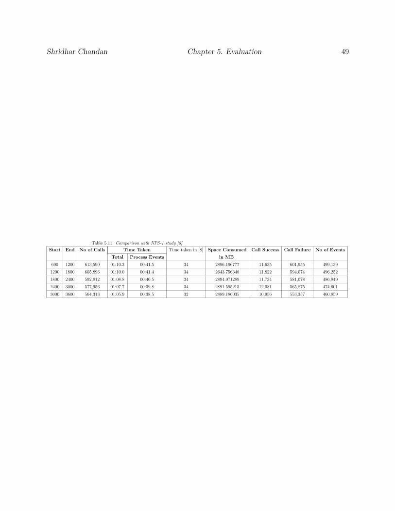
Shridhar Chandan Chapter 5. Evaluation 49
Table 5.11: Comparison with NPS-1 study [8]
Start End No of Calls Time Taken Time taken in [8] Space Consumed Call Success Call Failure No of Events
Total Process Events in MB
600 1200 613,590 01:10.3 00:41.5 34 2896.196777 11,635 601,955 499,139
1200 1800 605,896 01:10.0 00:41.4 34 2643.756348 11,822 594,074 496,252
1800 2400 592,812 01:08.8 00:40.5 34 2894.071289 11,734 581,078 486,849
2400 3000 577,956 01:07.7 00:39.8 34 2891.595215 12,081 565,875 474,601
3000 3600 564,313 01:05.9 00:38.5 32 2889.186035 10,956 553,357 460,859

Chapter 6
Conclusion and Future Work
We have presented a realistic framework for modeling mobility and cellular traffic given the
profiles of callers, call traffic, call behavior, and mobility representation for a study area. The
tool is capable of capturing the most important time sensitive and dynamic characteristics
of mobile network traffic at a large urban scale. The framework is suitable for simulating
complex events, and it also supports database connectivity. The tool is easily extensible
through the addition of new events while minimizing impact to existing system functions.
We have evaluated the system on various input data sets and various parameters for its
performance, efficiency, and consistency. We have also examined the system during complex
network topology changes, and the impact of these changes on mobility and calling patterns.
The simulation results are promising and show that this framework can be instrumental in
contingency planning and spectrum allocation applications. This framework provides policy
makers with the ability to plan various disaster recovery strategies. We believe that tools
such as Diamond will be critical in effective management of the dynamic wireless spectrum
in next generation networks.
6.1 Future Work
There are many potential improvements to Diamond. Some of these ideas are:
50

Shridhar Chandan Chapter 6. Conclusion and Future Work 51
• Currently Diamond supports sequential processing. In order to analyze more complex
networks, parallel and distributed computation is preferable.
• EBR can be sent to persons from a specified cell only. This feature can be helpful to
send EBR only in cell tower outage area.
• Cell towers that can cover any polygonal shape.
• The addition of cell towers in a Cell Tower Up event.
• Simulating wireless ad-hoc networks, where a set of mobile devices, called nodes, with
processing and wireless transmission capabilities powered by on-board batteries can
communicate with each other. In a mobile ad-hoc network, nodes must cooperate to
dynamically establish routes using multi-hop wireless links. There is no stationary
infrastructure, and each node acts as a router. Every node is associated to a single
user which moves inside the environment. Therefore, node mobility patterns depend
on the characteristics of both the users and the environment [47].

Bibliography
[1] FCC Antenna Registration System. http://wireless.fcc.gov/antenna/index.htm?
job=home/.
[2] Simple, Thread-safe Approximate Nearest Neighbor (STANN). https://sites.
google.com/a/compgeom.com/stann/.
[3] TowerMaps. http://www.towermaps.com/.
[4] Planning guidance for response to a nuclear detonation, 2009.
[5] Qing an Zeng and Dharma P. Agrawal. Handoff in wireless mobile networks. http:
//cis.temple.edu/~wu/teaching/Spring%202013/handoff.pdf.
[6] Anand Balachandran, Geoffrey M. Voelker, Paramvir Bahl, and P. Venkat Rangan.
Characterizing user behavior and network performance in a public wireless lan. In
ACM SIGMETRICS, 2002.
[7] C. L. Barrett, R. J. Beckman, K. P. Berkbigler, K. R. Bisset, B. W. Bush, K. Campbell,
S. Eubank, K. M. Henson, J. M. Hurford, D. A. Kubicek, M. V. Marathe, P. R. Romero,
J. P. Smith, L. L. Smith, P. L. Speckman, P. E. Stretz, G. L. Thayer, E. V. Eeckhout,
and M. D. Williams. Transims: Transportation analysis simulation system. Technical
Report LA-UR-00-1725, Los Alamos National Laboratory, 1997.
[8] Christopher Barrett, Keith Bisset, Shridhar Chandan, Jiangzhuo Chen, Youngyun
Chungbaek, Stephen Eubank, Yaman Evrenosoglu, Bryan Lewis, Kristian Lum, Achla
Marathe, et al. Planning and response in the aftermath of a large crisis: An agent-based
informatics framework.
52

Shridhar Chandan Chapter 6. Conclusion and Future Work 53
[9] Christopher L. Barrett, Richard J. Beckman, Maleq Khan, V. S. Anil Kumar, Mad-
hav V. Marathe, Paula E. Stretz, Tridib Dutta, and Bryan Lewis. Generation and
analysis of large synthetic social contact networks. In Winter Simulation Conference,
WSC ’09, pages 1003–1014. Winter Simulation Conference, 2009.
[10] Christopher L Barrett, Stephen Eubank, Achla Marathe, Madhav V Marathe,
Zhengzheng Pan, and Samarth Swarup. Information integration to support model-
based policy informatics. The innovation journal: the public sector innovation journal,
16(1), 2011.
[11] C.L. Barrett, K. Bisset, S. Eubank, V. S. Anil Kumar, M.V. Marathe, and H.S. Mortveit.
Modeling and Simulation of Large Biological, Information and Socio-Technical Systems:
An Interaction-Based Approach. In Proceedings of the Short Course on Modeling and
Simulation of Biological Networks, pages 353–392. Springer Berlin Heidelberg, 2006.
[12] R. Beckman, K. Channakeshava, Fei Huang, V.S.A. Kumar, A. Marathe, M.V. Marathe,
and Guanhong Pei. Synthesis and analysis of spatio-temporal spectrum demand pat-
terns: A first principles approach. In Proceedings of IEEE Symposium on New Frontiers
in Dynamic Spectrum Access Networks, pages 1 – 12, Singapore, 2010. IEEE.
[13] Richard Beckman, Karthik Channakeshava, Fei Huang, V. S. Anil Kumar, Achla
Marathe, Madhav V. Marathe, and Guanhong Pei. Implications of dynamic spectrum
access on the efficiency of primary wireless market. In IEEE DySpan, 2010.
[14] Richard J Beckman, Keith A Baggerly, and Michael D McKay. Creating synthetic
baseline populations. Transportation Research Part A: Policy and Practice, 30(6):415–
429, 1996.
[15] Richard J. Beckman, Karthik Channakeshava, Fei Huang, Junwhan Kim, Achla
Marathe, Madhav V. Marathe, Guanhong Pei, Sudip Saha, and Anil Kumar S. Vul-
likanti. Integrated multi-network modeling environment for spectrum management.
IEEE Journal on Selected Areas in Communications, 31(6):1158–1168, 2013.
[16] Russell Bent, Stephan Eidenbenz, and Sunil Thulasidasan. Large-scale telephone net-
work simulation: discrete event vs. steady state. In Wainer et al. [48].

Shridhar Chandan Chapter 6. Conclusion and Future Work 54
[17] Azzedine Boukerche, Sajal K. Das, and Alessandro Fabbri. Swimnet: A scalable par-
allel simulation testbed for wireless and mobile networks. Wirel. Netw., 7(5):467–486,
September 2001.
[18] Valentine J.E. Millage K.K. Brandt L.D. Buddemeier, B.R. National Capital Region:
Key response planning factors for the aftermath of nuclear terrorism., 2011.
[19] Barrett C., R. Beckman, K. Channakeshava, Fei Huang, V.S.A. Kumar, A. Marathe,
M.V. Marathe, and Guanhong Pei. Cascading failures in multiple infrastructures: From
transportation to communication network. In Proceedings of Interacting Critical Infras-
tructures for the 21st Century, pages 20–22, Beijing, China, 2010. IEEE.
[20] T. Camp, J. Boleng, and V. Davies. A survey of mobility models for ad hoc network
research. Wireless Communications and Mobile Computing (WCMC): Special issue on
Mobile Ad Hoc Networking: Research, Trends and Applications, pages 483–502, 2002.
[21] Center for Disease Control. National Health Interview Survey (NHIS). http://www.
cdc.gov/nchs/about/major/nhis/nhis_2007_data_release.htm.
[22] Shridhar Chandan, Sudip Saha, Christopher L. Barrett, Stephen Eubank, Achla
Marathe, Madhav V. Marathe, Samarth Swarup, and Anil Kumar S. Vullikanti. Model-
ing the interaction between emergency communications and behavior in the aftermath
of a disaster. In Greenberg et al. [31], pages 476–485.
[23] Fei Huang Junwhan Kim Achla Marathe Madhav V. Marathe Guanhong Pei Sudip Saha
Balaaji S. P. Subbiah Anil Kumar S. Vullikanti Chris Barrett, Karthik Channakeshava.
Human initiated cascading failures in societal infrastructures. Number 10, 2012.
[24] Michael Connor and Piyush Kumar. Fast construction of k-nearest neighbor graphs for
point clouds. IEEE Trans. Vis. Comput. Graph., 16(4):599–608, 2010.
[25] D.C. Cox. Wireless personal communications: what is it? Personal Communications,
IEEE, 2(2):20–35, 1995.
[26] Paul Currion, Chamindra de Silva, and Bartel Van de Walle. Open source software for
disaster management. Commun. ACM, 50(3):61–65, March 2007.

Shridhar Chandan Chapter 6. Conclusion and Future Work 55
[27] S. Eubank, H. Guclu, V. S. Anil Kumar, M.V. Marathe, A. Srinivasan, Z. Toroczkai,
and N. Wang. Modeling disease outbreaks in realistic urban social networks. Nature,
429(6998):180–184, 2004.
[28] Richard M. Fujimoto. Parallel and Distribution Simulation Systems. John Wiley &
Sons, Inc., New York, NY, USA, 1st edition, 1999.
[29] R.M. Fujimoto. Parallel and distributed simulation systems. In Simulation Conference,
2001. Proceedings of the Winter, volume 1, pages 147–157 vol.1, 2001.
[30] Marta C. Gonzalez, Cesar A Hidalgo, and Albert-Laszlo Barabasi. Understanding in-
dividual human mobility patterns. Nature, 453:779–782, 2008.
[31] Ariel M. Greenberg, William G. Kennedy, and Nathan Bos, editors. Social Computing,
Behavioral-Cultural Modeling and Prediction - 6th International Conference, SBP 2013,
Washington, DC, USA, April 2-5, 2013. Proceedings, volume 7812 of Lecture Notes in
Computer Science. Springer, 2013.
[32] A. Jardosh, E. Belding-Royer, K. Almeroth, and S. Suri. Towards realistic mobility
models for mobile ad hoc networks. In ACM MobiCom, 2003.
[33] Junwhan Kim, V. S. Anil Kumar, Achla Marathe, Guanhong Pei, Sudip Saha, and Bal-
aaji S.P. Subbiah. Modeling cellular network traffic with mobile call graph constraints.
In Proceedings of Winter Simulation Conference. IEEE, 2011.
[34] David Kotz and Kobby Essien. Analysis of a campus-wide wireless network. Wireless
Networks, 2005.
[35] L. Kroc, S. Eidenbenz, and J. Smith. Sessionsim: Activity-based session generation for
network simulation. In Winter Simulation Conference, 2009.
[36] Derek Lam, Donald C. Cox, and Jennifer Widom. Teletraffic modeling for personal
communications services. IEEE COMMUNICATIONS MAGAZINE, 35:79–87, 1997.
[37] Hyunok Lee, V. Manshadi, D.C. Cox, and N.K. Cheung. High fidelity simulation of
mobile cellular systems with integrated resource allocation and adaptive antennas. In
Wireless Communications and Networking Conference, 2007.WCNC 2007. IEEE, pages
3210–3215, 2007.

Shridhar Chandan Chapter 6. Conclusion and Future Work 56
[38] Amit A. Nanavati, Siva Gurumurthy, Gautam Das, Dipanjan Chakraborty, Koustuv
Dasgupta, Sougata Mukherjea, and Anupam Joshi. On the structural properties of
massive telecom call graphs: findings and implications. In Proceedings of the 15th ACM
international conference on Information and knowledge management, CIKM ’06, pages
435–444, New York, NY, USA, 2006. ACM.
[39] Network Dynamics and Simulation Science Lab, Virginia Tech. Synthetic data products
for societal infrastructures and proto-populations. ndssl.vbi.vt.edu/opendata.
[40] David M. Nicol, Michael M. Johnson, and Ann S. Yoshimura. The ides framework: A
case study in development of a parallel discrete-event simulation system. In Proceedings
of the 29th Conference on Winter Simulation, WSC ’97, pages 93–99, Washington, DC,
USA, 1997. IEEE Computer Society.
[41] Nidhi Parikh, Samarth Swarup, Paula E. Stretz, Caitlin M. Rivers, Bryan L. Lewis,
Madhav V. Marathe, Stephen G. Eubank, Christopher L. Barrett, Kristian Lum, and
Youngyun Chungbaek. Modeling human behavior in the aftermath of a hypothetical
improvised nuclear detonation. In Proceedings of the 2013 international conference on
Autonomous agents and multi-agent systems, AAMAS ’13, pages 949–956, Richland,
SC, 2013. International Foundation for Autonomous Agents and Multiagent Systems.
[42] Venkatesh Ramaswamy, S. Thulasidasan, Phil Romero, S. Eidenbenz, and L. Cuellar.
Simulating the national telephone network: A socio-technical approach to assessing in-
frastructure criticality. In Military Communications Conference, 2007. MILCOM 2007.
IEEE, pages 1–7, 2007.
[43] Mukund Seshadri, Sridhar Machiraju, Ashwin Sridharan, Jean Bolot, Christos Falout-
sos, and Jure Leskove. Mobile Call Graphs: Beyond Power-law and Lognormal Distri-
butions. In KDD ’08: Proceeding of the 14th ACM SIGKDD international conference
on Knowledge discovery and data mining, pages 596–604. ACM, 2008.
[44] A.M. Seybold. The big question: Why do we need more cell sites? http://files.
ctia.org/pdf/Why_Do_We_Need_More_Cell_Sites.pdf, 2010.
[45] D. Tang and M. Baker. Analysis of a local-area wireless network. In ACM MobiCom,
pages 1–10, 2000.

Shridhar Chandan Chapter 6. Conclusion and Future Work 57
[46] Sunil Thulasidasan and Stephan Eidenbenz. Accelerating traffic microsimulations: A
parallel discrete-event queue-based approach for speed and scale. In Winter Simulation
Conference, WSC ’09, pages 2457–2466. Winter Simulation Conference, 2009.
[47] David Tipper, Yi Qian, and Xiaobing Hou. Modeling the time varying behavior of
mobile ad-hoc networks. In Simonetta Balsamo, Carla-Fabiana Chiasserini, and Lorenzo
Donatiello, editors, MSWiM, pages 12–19. ACM, 2004.
[48] Gabriel A. Wainer, Clifford A. Shaffer, Robert M. McGraw, and Michael J. Chinni,
editors. Proceedings of the 2009 Spring Simulation Multiconference, SpringSim 2009,
San Diego, California, USA, March 22-27, 2009. SCS/ACM, 2009.
[49] Choi Y. Denuit S. Wein, L.M. Analyzing evacuation versus shelter-in-place strategies
after a terrorist nuclear detonation. 2010.
[50] D. Willkomm, S. Machiraju, J. Bolot, and A. Wolisz. Primary users in cellular networks:
A large-scale measurement study. In IEEE DySPAN, pages 1–11, Oct. 2008.
[51] Bernard P. Zeigler. Theory of Modeling and Simulation. John Wiley, 1976.