Discrete Differential Forms for Computational Modelingkanso/papers/DeKaTo2007.pdf · Discrete Differential Forms for Computational Modeling Mathieu Desbrun, Eva Kanso and Yiying Tong

Discrete Differential Formsfor Computational Modeling

Mathieu Desbrun, Eva Kanso and Yiying Tong

Abstract. This chapter introduces the background needed to develop a geometry-based, principled approach to computational modeling. We show that the use of dis-crete differential forms often resolves the apparent mismatch between differential anddiscrete modeling, for applications varying from graphics to physical simulations.

1. Motivationix: differential form—(

The emergence of computers as an essential tool in scientific research has shaken the veryfoundations of differential modeling. Indeed, the deeply-rooted abstraction of smooth-ness, or differentiability, seems to inherently clash with a computer’s ability of storingonly finite sets of numbers. While there has been a series of computational techniquesthat proposed discretizations of differential equations, the geometric structures they aresimulating are often lost in the process.

1.1. The role of geometry in scienceGeometry is the study of space and of the properties of shapes in space. Dating back toEuclid, models of our surroundings have been formulated using simple, geometric de-scriptions, formalizing apparent symmetries and experimental invariants. Consequently,geometry is at the foundation of many current physical theories: general relativity, elec-tromagnetism (E&M), gauge theory as well as solid and fluid mechanics all have strongunderlying geometrical structures. Einstein’s theory for instance states that gravitationalfield strength is directly proportional to the curvature of space-time. In other words, thephysics of relativity is directly modelled by the shape of our 4-dimensional world, just asthe behavior of soap bubbles is modeled by their shapes. Differential geometry is thus, defacto, the mother tongue of numerous physical and mathematical theories.

Unfortunately, the inherent geometric nature of such theories is often obstructedby their formulation in vectorial or tensorial notations: the traditional use of a coordi-nate system, in which the defining equations are expressed, often obscures the underlying

2 Mathieu Desbrun, Eva Kanso and Yiying Tong

structures by an overwhelming usage of indices. Moreover, such complex expressionsentangle the topological and geometrical content of the model.

1.2. Geometry-based exterior calculusThe geometric nature of these models is best expressed and elucidated through the use ofthe exterior calculus of differential forms, first introduced by Cartan [7]. This geometry- ix: exterior calculus

based calculus was further developed and refined over the twentieth century to becomethe foundation of modern differential geometry. The calculus of exterior forms allows oneto express differential and integral equations on smooth and curved spaces in a consistentmanner, while revealing the geometrical invariants at play. For example, the classicaloperations of gradient, divergence, and curl as well as the theorems of Green, Gauss andStokes can all be expressed concisely in terms of differential forms and an operator onthese forms called the exterior derivative—hinting at the generality of this approach.

Compared to classical tensorial calculus, this exterior calculus has several advan-tages. First, it is often difficult to recognize the coordinate-independent nature of quan-tities written in tensorial notation: local and global invariants are hard to notice by juststaring at the indices. On the other hand, invariants are easily discovered when expressedas differential forms by invoking either Stokes’ theorem, the Poincare lemma, or by apply-ing exterior differentiation. Note also that the exterior derivative of differential forms—theantisymmetric part of derivatives—is one of the most important parts of differentiation,since it is invariant under coordinate system change. In fact, Sharpe states in [37] thatevery differential equation may be expressed in term of the exterior derivative of differ-ential forms. As a consequence, several recent initiatives have been aimed at formulatingphysical laws in terms of differential forms. For recent work along these lines, the readeris invited to refer to [5, 1, 27, 13, 32, 6, 16] for books offering a theoretical treatment ofvarious physical theories using differential forms.

1.3. Differential vs. discrete modelingWe have seen that a large amount of our scientific knowledge relies on a deeply-rooteddifferential (i.e., smooth) comprehension of the world. This abstraction of differentiabilityallows researchers to model complex physical systems via concise equations. With thesudden advent of the digital age, it was therefore only natural to resort to computationsbased on such differential equations.

However, since digital computers can only manipulate finite sets of numbers, theircapabilities seem to clash with the basic foundations of differential modeling. In order toovercome this hurdle, a first set of computational techniques (e.g., finite difference or par-ticle methods) focused on satisfying the continuous equations at a discrete set of spatialand temporal samples. Unfortunately, focusing on accurately discretizing the local lawsoften fails to respect important global structures and invariants. Later methods such asFinite Elements (FEM), drawing from developments in the calculus of variations, reme-died this inadequacy to some extent by satisfying local conservation laws on average andpreserving some important invariants. Coupled with a finer ability to deal with arbitraryboundaries, FEM became the de facto computational tool for engineers. Even with signif-icant advances in error control, convergence, and stability of these finite approximations,

Discrete Differential Forms for Computational Modeling 3

the underlying structures of the simulated continuous systems are often destroyed: a mov-ing rigid body may gain or loose momentum; or a cavity may exhibit fictitious eigenmodesin an electromagnetism (E&M) simulation. Such examples illustrate some of the loss offidelity that can follow from a standard discretization process, failing to preserve somefundamental geometric and topological structures of the underlying continuous models.

The cultural gap between theoretical and applied science communities may be par-tially responsible for the current lack of proper discrete, computational modeling thatcould mirror and leverage the rich developments of its differential counterpart. In par-ticular, it is striking that the calculus of differential forms has not yet had an impact onthe mainstream computational fields, despite excellent initial results in E&M [4] or La-grangian mechanics [29]. It should also be noticed that some basic tools necessary forthe definition of a discrete calculus already exist, probably initiated by Poincare when hedefined his cell decomposition of smooth manifolds. The study of the structure of orderedsets or simplices now belongs to the well-studied branch of mathematics known as Com-binatorial Differential Topology and Geometry, which is still an active area of research(see, e.g., [15] and [2] and references therein).

1.4. Calculus ex geometricaGiven the overwhelming geometric nature of the most fundamental and successful calcu-lus of these last few centuries, it seems relevant to approach computations from a geomet-ric standpoint.

One of the key insights that percolated down from the theory of differential formsis rather simple and intuitive: one needs to recognize that different physical quantitieshave different properties, and must be treated accordingly. Fluid mechanics or electro-magnetism, for instance, make heavy use of line integrals, as well as surface and volumeintegrals; even physical measurements are performed as specific local integrations or av-erages (think flux for magnetic field, or current for electricity, or pressure for atoms’collisions). Pointwise evaluations or approximations for such quantities are not the appro-priate discrete analogs, since the defining geometric properties of their physical meaningcannot be enforced naturally. Instead, one should store and manipulate those quantitiesat their geometrically-meaningful location: in other words, we should consider values onvertices, edges, faces, and tetrahedra as proper discrete versions of respectively pointwisefunctions, line integrals, surface integrals, and volume integrals: only then will we be ableto manipulate those values without violating the symmetries that the differential modelingtried to exploit for predictive purposes.

1.5. Similar endeavorsThe need for improved numerics have recently sprung a (still limited) number of interest-ing related developments in various fields. Although we will not try to be exhaustive, wewish to point the reader to a few of the most successful investigations with the same “fla-vor” as our discrete geometry-based calculus, albeit their approaches are rarely similar toours. First, the field of Mimetic Discretizations of Continuum Mechanics, led by Shashkov,Steinberg, and Hyman [24], started on the premise that spurious solutions obtained from


finite element or finite difference methods often originate from inconsistent discretiza-tions of the operators div, curl, and grad, and that addressing this inconsistency pays offnumerically. Similarly, Computational Electromagnetism has also identified the issue offield discretization as the main reason for spurious modes in numerical results. An excel-lent treatment of the discretization of the Maxwell’s equations resulted [4], with a clearrelationship to the differential case. Finally, recent developments in Discrete LagrangianMechanics have demonstrated the efficacy of a proper discretization of the Lagrangianof a dynamical system, rather than the discretization of its derived Euler–Lagrange equa-tions: with a discrete Lagrangian, one can ensure that the integration scheme satisfies anexact discrete least-action principle, preserving all the momenta directly for arbitrary or-ders of accuracy [29]. Respecting the defining geometric properties of both the fields andthe governing equations is a common link between all these recent approaches.

1.6. Advantages of discrete differential modelingThe reader will have most probably understood our bias by now: we believe that thesystematic construction, inspired by Exterior Calculus, of differential, yet readily dis-cretizable computational foundations is a crucial ingredient for numerical fidelity. Be-cause many of the standard tools used in differential geometry have discrete combinato-rial analogs, the discrete versions of forms or manifolds will be formally identical to (andshould partake of the same properties as) the continuum models. Additionally, such anapproach should clearly maintain the separation of the topological (metric-independent)and geometrical (metric-dependent) components of the quantities involved, keeping thegeometric picture (i.e., intrinsic structure) intact.

A discrete differential modeling approach to computations will also be often muchsimpler to define and develop than its continuous counterpart. For example, the discretenotion of a differential form will be implemented simply as values on mesh elements.Likewise, the discrete notion of orientation will be more straightforward than its contin-uous counterpart: while the differential definition of orientation uses the notion of equiv-alence class of atlases determined by the sign of the Jacobian, the orientation of a meshedge will be one of two directions; a triangle will be oriented clockwise or counterclock-wise; a volume will have a direction as a right-handed helix or a left-handed one; no notionof atlas (a collection of consistent coordinate charts on a manifold) will be required.

1.7. Goal of this chapterGiven these premises, this chapter was written with several purposes in mind. First, wewish to demonstrate that the foundations on which powerful methods of computations canbe built are quite approachable—and are not as abstract as the reader may fear: the ideasinvolved are very intuitive as a side effect of the simplicity of the underlying geometricprinciples.

Second, we wish to help bridge the gap between applied fields and theoretical fields:we have tried to render the theoretical bases of our exposition accessible to computer sci-entists, and the concrete implementation insights understandable by non-specialists. Forthis very reason, the reader should not consider this introductory exposition as a definitesource of knowledge: it should instead be considered as a portal to better, more focused


FIGURE 1. Typical 2D and 3D meshes: although the David head ap-pears smooth, its surface is made of a triangle mesh; tetrahedral meshes(such as this mechanical part, with a cutaway view) are some typicalexamples of irregular meshes on which computations are performed.David’s head mesh is courtesy of Marc Levoy, Stanford.

work on related subjects. We only hope that we will ease our readers into foundationalconcepts that can be undoubtedly and fruitfully applied to all sorts of computations—beit for graphics or simulation.

With these goals in mind, we will describe the background needed to develop a prin-cipled, geometry-based approach to computational modeling that gets around the apparentmismatch between differential and discrete modeling.

2. Relevance of forms for integrationThe evaluation of differential quantities on a discrete space (mesh) is a nontrivial prob-lem. For instance, consider a piecewise-linear 2-dimensional surface embedded in a three-dimensional Euclidean space, i.e., a triangle mesh. Celebrated quantities such as theGaussian and mean curvatures are delicate to define on it. More precisely, the Gauss-ian curvature can be easily proven to be zero everywhere except on vertices, where it isa Dirac delta function. Likewise, the mean curvature can only be defined in the distribu-tional sense, as a Dirac delta function on edges. However, through local integrations, onecan easily manipulate these quantities numerically: if a careful choice of non-overlappingregions is made, the delta functions can be properly integrated, rendering the computa-tions relatively simple as shown, for example, in [31, 22]. Note that the process of inte-gration to suppress discontinuity is, in spirit, equivalent to the idea of weak form used inthe Finite Element method.

This idea of integrated value has predated in some cases the equivalent differentialstatements: for instance, it was long known that the genus of a surface can be calcu-lated through a cell decomposition of the surface via the Euler characteristic. The actualGauss–Bonnet theorem was, however, derived later on. Now, if one tries to discretize the


Gaussian curvature of a piecewise-linear surface in an arbitrary way, it is not likely that itsintegral over the surface equals the desired Euler characteristic, while its discrete version,defined on vertices (or, more precisely, on the dual of each vertex), naturally preservesthis topological invariant.

2.1. From integration to differential formsIntegration is obviously a linear operation, since for any disjoint sets A and B,

∫

A∪B

=

∫

A

+

∫

B

.

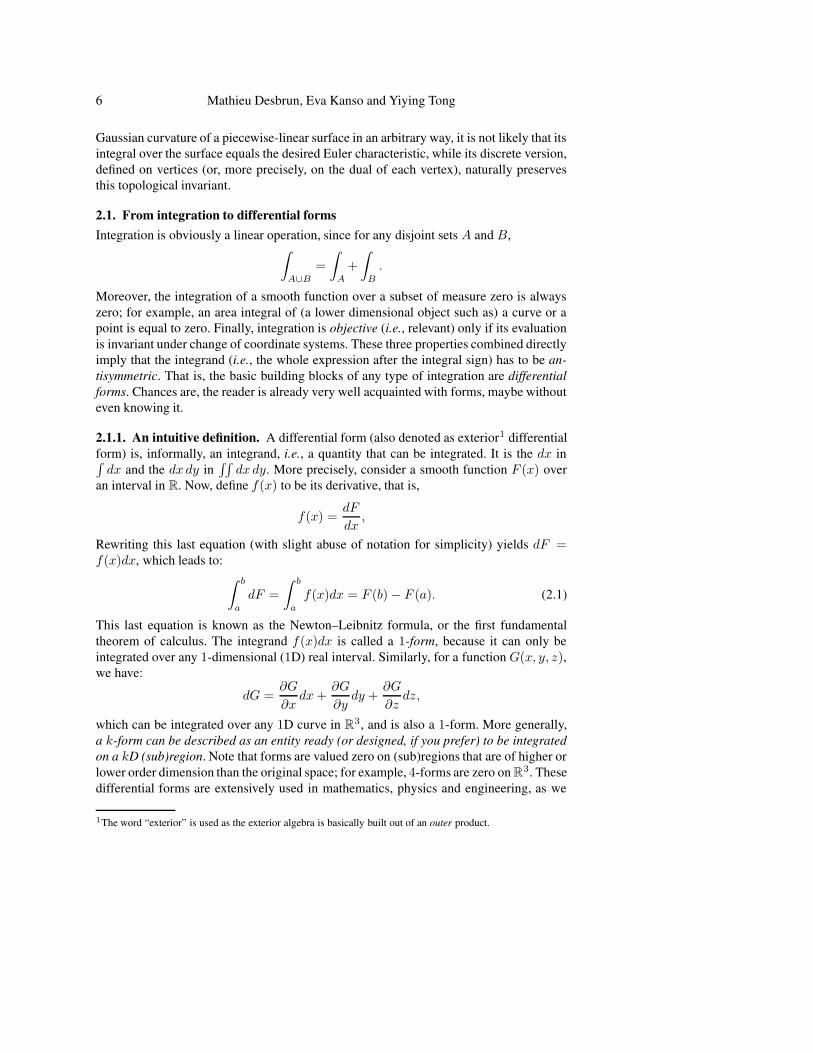
Moreover, the integration of a smooth function over a subset of measure zero is alwayszero; for example, an area integral of (a lower dimensional object such as) a curve or apoint is equal to zero. Finally, integration is objective (i.e., relevant) only if its evaluationis invariant under change of coordinate systems. These three properties combined directlyimply that the integrand (i.e., the whole expression after the integral sign) has to be an-tisymmetric. That is, the basic building blocks of any type of integration are differentialforms. Chances are, the reader is already very well acquainted with forms, maybe withouteven knowing it.

2.1.1. An intuitive definition. A differential form (also denoted as exterior1 differentialform) is, informally, an integrand, i.e., a quantity that can be integrated. It is the dx in∫

dx and the dx dy in∫∫

dx dy. More precisely, consider a smooth function F (x) overan interval in R. Now, define f(x) to be its derivative, that is,

f(x) =dF

dx,

Rewriting this last equation (with slight abuse of notation for simplicity) yields dF =f(x)dx, which leads to:

∫ b

a

dF =

∫ b

a

f(x)dx = F (b)− F (a). (2.1)

This last equation is known as the Newton–Leibnitz formula, or the first fundamentaltheorem of calculus. The integrand f(x)dx is called a 1-form, because it can only beintegrated over any 1-dimensional (1D) real interval. Similarly, for a function G(x, y, z),we have:

dG =∂G

∂xdx +

∂G

∂ydy +

∂G

∂zdz,

which can be integrated over any 1D curve in R3, and is also a 1-form. More generally,

a k-form can be described as an entity ready (or designed, if you prefer) to be integratedon a kD (sub)region. Note that forms are valued zero on (sub)regions that are of higher orlower order dimension than the original space; for example, 4-forms are zero on R

3. Thesedifferential forms are extensively used in mathematics, physics and engineering, as we

1The word “exterior” is used as the exterior algebra is basically built out of an outer product.


already hinted at the fact in Section 1.4 that most of our measurements ofthe world are of an integral nature: even digital pictures are made out oflocal area integrals of the incident light over each of the sensors of a camerato provide a set of values at each pixel on the final image (see inset). Theimportance of this notion of forms in science is also evidenced by the factthat operations like gradient, divergence, and curl can all be expressed interms of forms only, as well as fundamental theorems like Green’s or Stokes’.

2.1.2. A formal definition. For concreteness, consider the n-dimensional Euclidean spaceR

n, n ∈ IN and let M be an open regionM ⊂ Rn; M is also called an n-manifold.

The vector space TxM consists of all the (tangent) vectors at a point x ∈ M and can beidentified with R

n itself. A k-form ωk is a rank-k, antisymmetric tensor field overM.That is, at each point x ∈ M, it is a multi-linear map that takes k tangent vectors as inputand returns a real number:

ωk : TxM × · · · × TxM −→ R

which changes sign for odd permutations of the variables (hence the term antisymmetric).Any k-form naturally induces a k-form on a submanifold, through restriction of the linearmap to the domain that is the product of tangent spaces of the submanifold. ix: pseudoform

Comments on the notion of pseudoforms. There is a closely related concept namedpseudoform. Pseudo-forms change sign when we change the orientation of coordinate sys-tems, just like pseudovectors. As a result, the integration of a pseudoform does not changesign when the orientation of the manifold is changed. Unlike k-forms, a k-pseudoform in-duces a k-pseudoform on a submanifold only if a transverse direction is given. For exam-ple, fluid flux is sometimes called a 2-pseudoform: indeed, given a transverse direction,we know how much flux is going through a piece of surface; it does not depend on the ori-entation of the surface itself. Vorticity is, however, a true 2-form: given an orientation ofthe surface, the integration gives us the circulation around that surface boundary inducedby the surface orientation. It does not depend on the transverse direction of the surface.But if we have an orientation of the ambient space, we can always associate transversedirection with internal orientation of the submanifold. Thus, in our case, we may treatpseudoforms simply as forms because we can consistently choose a representative fromthe equivalence class.

2.2. The differential structureDifferential forms are the building blocks of a whole calculus. To manipulate these basicblocks, Exterior Calculus defines seven operators:

• d: the exterior derivative, that extends the notion of the differential of a function todifferential forms;

• ?: the Hodge star, that transforms k-forms into (n− k)–forms;• ∧: the wedge product, that extends the notion of exterior product to forms;• ] and [: the sharp and flat operators, that, given a metric, transform a 1-form into a

vector and vice-versa;


• iX : the interior product with respect to a vector field X (also called contractionoperator), a concept dual to the exterior product;

• LX : the Lie derivative with respect to a vector field X , that extends the notion ofdirectional derivative.

In this chapter, we will restrict our discussions to the first three operators, to provide themost basic tools necessary in computational modeling.

2.3. A taste of exterior calculus in R3

To give the reader a taste of the relative simplicity of Exterior Calculus, we provide alist of equivalences (in the continuous world!) between traditional operations and theirExterior Calculus counterpart in the special case of R

3. We will suppose that we have theusual Euclidean metric. Then, forms are actually quite simple to conceive:

0-form←→ scalar field1-form←→ vector field2-form←→ vector field3-form←→ scalar field

To be clear, we will add a superscript on the forms to indicate their rank. Thenapplying forms to vector fields amounts to:

1-form: u1(v)←→ u · v.2-form: u2(v, w) ←→ u · (v × w).3-form: f3(u, v, w)←→ fu · (v × w).

Furthermore, the usual operations like gradient, curl, divergence and cross productcan all be expressed in terms of the basic exterior calculus operators. For example:

d0f = ∇f , d1u = ∇× u, d2u = ∇ · u;?0f = f, ?1u = u, ?2u = u, ?3f = f ;?0d2 ?1 u1 = ∇ · u, ?1d1 ?2 u2 = ∇× u, ?2d0 ?3 f = ∇f ;f0 ∧ u = fu, u1 ∧ v1 = u× v, u1 ∧ v2 = u2 ∧ v1 = u · v;ivu

1 = u · v, ivu2 = u× v, ivf

3 = fv.

Now that we have established the relevance of differential forms even in the mostbasic vector operations, time has come to turn our attention to make this concept of formsreadily usable for computational purposes.

3. Discrete differential formsFinding a discrete counterpart to the notion of differential forms is a delicate matter. Ifone was to represent differential forms using their coordinate values and approximate theexterior derivative using finite differences, basic theorems such as Stokes theorem wouldnot hold numerically. The main objective of this section is therefore to present a properdiscretization of forms on what are known as simplicial complexes. We will show howthis discrete geometric structure, well suited for computational purposes, is designed topreserve all the fundamental differential properties. For simplicity, we restrict the dis-cussion to forms on 2D surfaces or 3D regions embedded in R

3, but the construction is


applicable to general manifolds in arbitrary spaces. In fact, the only necessary assumptionis that the embedding space must be a vector space, a natural condition in practice.

3.1. Simplicial complexes and discrete manifoldsFor the interested reader, the notions we introduce in this section are defined formallyin much more details (for the general case of k-dimensional spaces) in references suchas [33] or [21].

FIGURE 2. A 1-simplex is a line segment, the convex hull of twopoints. A 2-simplex is a triangle, i.e., the convex hull of three distinctpoints. A 3-simplex is a tetrahedron, as it is the convex hull of fourpoints.

3.1.1. Notion of simplex. A k-simplex is the generic term to describe the simplest meshelement of dimension k—hence the name. By way of motivation, consider a three-dimensionalmesh in space. This mesh is made of a series of adjacent tetrahedra (denoted tets for sim-plicity throughout). The vertices of the tets are called 0-simplices. Similarly, the line seg-ments or edges form a 1-simplices, the triangles or faces form 2-simplices, and the tetsform 3-simplices. Note that we can define these simplices in a top-down manner too: faces(2-simplices) can be thought of as boundaries of tets (3-simplices), edges (1-simplices) asboundaries of faces, and vertices (0-simplices) as boundaries of edges.

The definition of a simplex can be made more abstract as a series of k-tuples (re-ferring to the vertices they are built upon). However, for the type of applications that weare targeting in this chapter, we will often not make any distinction between an abstractsimplex and its topological realization (connectivity) or geometrical realization (positionsin space) .

Formally, a k-simplex σk is the nondegenerate convex hull of k + 1 geometricallydistinct points v0, . . . vk ∈ R

n with n ≥ k. In other words, it is the intersection of allconvex sets containing (v0, . . . vk); namely:

σk = x ∈ Rn|x =

k∑

i=0

αi vi with αi ≥ 0 and

k∑

i=0

αi = 1.

The entities v0, . . . vk are called the vertices and k is called the dimension of thek-simplex., which we will denote as:

σk = v0v1 · · · vk .


3.1.2. Orientation of a simplex. Note that all orderings of the k + 1 vertices of a k-simplex can be divided into two equivalent classes, i.e., two orderings differing by aneven permutation. Such a class of orderings is called an orientation. In the present work,we always assume that local orientations are given for each simplex; that is, each elementof the mesh has been given a particular orientation. For example, an edge σ1 = v0v1in Figure 2 has an arrow indicating its default orientation. If the opposite orientation isneeded, we will denote it as v1v0, or, equivalently, by −v0v1. For more details andexamples, the reader is referred to [33, 23].

3.1.3. Boundary of a simplex. Any (k−1)–simplex spanned by a subset of v0, . . . vkis called a (k−1)–face of σk. That is, a (k−1)–face is simply a (k−1)–simplex whose kvertices are all from the k +1 vertices of the k-simplex. The union of the (k− 1)–faces iswhat is called the boundary of the k-simplex. One should be careful here: because of thedefault orientation of the simplices, the formal signed sum of the (k − 1)–faces definesthe boundary of the k-simplex. Therefore, the boundary operator takes a k-simplex andgives the sum of all its (k − 1)–faces with 1 or −1 as coefficients depending on whethertheir respective orientations match or not, see Figure 4.

FIGURE 3. The boundary operator ∂ applied to a triangle (a 2-simplex)is equal to the signed sum of the edges (i.e., the 1-faces of the 2-simplex).

To remove possible mistakes in orientation, we can define the boundary operator asfollows:

∂v0v1 · · · vk =

k∑

j=0

(−1)jv0, . . . , vj , . . . , vk, (3.1)

where vj indicates that vj is missing from the sequence, see Figure 3. Clearly, each k-simplex has k + 1 facets or (k − 1)–faces. For this statement to be valid even for k = 0,the empty set ∅ is usually defined as a (−1)–simplex face of every 0-simplex. The readeris invited to verify this definition on the triangle v0, v1, v2 in Figure 3:

∂v0, v1, v2 = v1, v2 − v0, v2+ v0, v1

ix: simplicial complex

3.1.4. Simplicial complex. A simplicial complex is a collection K of simplices, whichsatisfies the following two simple conditions:• every face of each simplex in K is in K;• the intersection of any two simplices inK is either empty, or an entire common face.

Computer graphics makes heavy use of what is called realizations of simplicialcomplexes. Loosely speaking, a realization of a simplicial complex is an embedding ofthis complex into the underlying space R

n. Triangle meshes in 2D and tet meshes in 3D


FIGURE 4. Boundary operator applied to a triangle (left), and a tetra-hedron (right). Orientations of the simplices are indicated with arrows.

are examples of such simplicial complexes (see Figure 1). Notice that polygonal meshescan be easily triangulated, thus can be easily turned into simplicial complexes. One canalso use the notion of cell complex by allowing the elements of K to be non-simplicial;we will restrict our explanations to the case of simplicial complexes for simplicity.

ix: discrete manifold

3.1.5. Discrete manifolds. An n-dimensional discrete manifoldM is an n-dimensionalsimplicial complex that satisfies the following condition: for each simplex, the union of allthe incident n-simplices forms an n-dimensional ball (i.e., a disk in 2D, a ball in 3D, etc),or half a ball if the simplex is on the boundary. As a consequence, each (n− 1)–simplexhas exactly two adjacent n-simplices—or only one if it is on a boundary.

Basically, the notion of discrete manifold corresponds to the usual Computer Graph-ics acceptation of “manifold mesh”. For example in 2D, discrete manifolds cannot haveisolated edges (also called sticks or hanging edges) or isolated vertices, and each of theiredges is adjacent to 2 triangles (except for the boundary; in that case, the edge is adjacentto only one triangle). A surface mesh in 3D cannot have a “fin”, i.e., an edge with morethan two adjacent triangles. To put it differently, infinitesimally-small, imaginary inhab-itants of a n-dimensional discrete manifolds would consider themselves living in R

n asany small neighborhood of this manifold is isomorphic to R

n.

3.2. Notion of chains ix: chain complex

We have already encountered the notion of chain, without mentioning it. Recall that theboundary operator takes each k-simplex and gives the signed sum of all its (k − 1)–faces. We say that the boundary of a k-simplex produces a (k − 1)–chain. The followingdefinition is more precise and general.

3.2.1. Definition. A k-chain of an oriented simplicial complex K is a set of values, onefor each k-simplex ofK. That is, a k-chain c can then be thought of as a linear combinationof all the k-simplices in K:

c =∑

σ∈K

c(σ) · σ, (3.2)

where c(σ) ∈ R. We will denote the group of all k-chains as Ck.


FIGURE 5. (a) A simplicial complex consisting of all verticesv0, v1, v2, v3 and edges e0, e1, e2, e3, e4. This simplicial complexis not a discrete manifold because the neighborhoods of the vertices v1

and v2 are not 1D balls. (b) If we add the triangles f0 and f1 to thesimplicial complex, it becomes a 2-manifold with one boundary.

3.2.2. Implementation of chains. Let the set of all k-simplices inK be denotedKk , andlet its cardinality be denoted as |Kk |. A k-chain can simply be stored as a vector (or array)of dimension |Kk|, i.e., one number for each k-simplex σk ∈ Kk .

3.2.3. Boundary operator on chains. We mentioned that the boundary operator ∂ wasreturning a particular type of chain, namely, a chain with coefficients equal to either 0, 1,or−1. Therefore, it should not be surprising that we can extend the notion of boundary toact also on k-chains, simply by linearity:

∂∑

k

ckσk =∑

k

ck∂σk.

That is, from one set of values assigned to all simplices of a complex, one can deduce

FIGURE 6. (a) An example of 1-chain being the boundary of a face(2-simplex); (b) a second example of 1-chain with 4 nonzero coeffi-cients.

another set of values derived by weighting the boundaries of each simplex by the originalvalue stored on it. This operation is very natural, and can thus be implemented easily asexplained next.

3.2.4. Implementation of the boundary operator. Since the boundary operator is alinear mapping from the space of k-simplices to the space of (k − 1)–simplices, it cansimply be represented by a matrix of dimension |Kk−1| × |Kk|. The reader can convinceherself that this matrix is sparse, as only immediate neighbors are involved in the boundaryoperator. Similarly, this matrix contains only the values 0, 1, and −1. Notice that in 3D,


there are three nontrivial boundary operators ∂k (∂1 is the boundary operator on edges,∂2 on triangles, ∂3 on tets). However, the operator needed for a particular operation isobvious from the type of the argument: if the boundary of a tet is needed, the operator ∂3

is the only one that makes sense to apply; in other words, the boundary of a k-simplexσk is found by invoking ∂kσk . Thanks to this context-dependence, we can simplify thenotation and remove the subscript when there is no ambiguity.

3.3. Notion of cochains ix: cochain, coboundary

A k-cochain ω is the dual of a k-chain, that is to say, ω is a linear mapping that takesk-chains to R. One writes:

ω : Ck → R

c → ω(c), (3.3)

which reads as: a k-cochain ω operates on a k-chain c to give a scalar in R. Since a chainis a linear combination of simplices, a cochain returns a linear combination of the valuesof that cochain on each simplex involved.

Clearly, a cochain also corresponds to one value per simplex (since all the k-simplicesform a basis for the vector space Ck, and we only need to know the mapping of vectors inthis basis to determine a linear mapping), and hence the notion of duality of chains andcochains is appropriate. But contrary to a chain, a k-cochain is evaluated on each simplexof the dimension k. In other words, a k-cochain can be thought of as a field that can beevaluated on each k-simplex of an oriented simplicial complex K.

3.3.1. Implementation of cochains. The numerical representation of cochains followsfrom that of chains by duality. Recall that a k-chain can be represented as a vector ck

of length equal to the number of k-simplices inM. Similarly, one may represent ω by avector ωk of the same size as ck.

Now, remember that ω operates on c to give a scalar in R. The linear operation ω(c)translates into an inner product ωk · ck. More specifically, one may continue to think ofck as a column vector so that the R-valued linear mapping ω can be represented by a rowvector (ωk)t, and ω(c) becomes simply the matrix multiplication of the row vector (ωk)t

with the column vector ck. The evaluation of a cochain is therefore trivial to implement.

3.4. Discrete forms as cochainsThe attentive reader will have noticed by now: k-cochains are discrete analogs to dif-ferential forms. Indeed, a continuous k-form was defined as a linear mapping from k-dimensional sets to R, as we can only integrate a k-form on a k-(sub)manifold. Note nowthat a kD set, when one has only a mesh to work with, is simply a chain. And a linearmapping from a chain to a real number is what we called a cochain: a cochain is thereforea natural discrete counterpart of a form.

For instance a 0-form can be evaluated at each point, a 1-form can be evaluated oneach curve, a 2-form can be evaluated on each surface, etc. Now if we restrict integrationto take place only on the k-submanifold which is the sum of the k-simplices in the tri-angulation, we get a k-cochain; thus k-cochains are a discretization of k-forms. One canfurther map a continuous k-form to a k-cochain. To do this, first integrate the k-form on


each k-simplex and assign the resulting value to that simplex to obtain a k-cochain on thek-simplicial complex. This k-cochain is a discrete representation of the original k-form.

3.4.1. Evaluation of a form on a chain. We can now naturally extend the notion ofevaluation of a differential form ω on an arbitrary chain simply by linearity:

∫∑

i ciσi

ω =∑

i

ci

∫

σi

ω. (3.4)

As mentioned above, the integration of ω on each k-simplex σk provides a discretizationof ω or, in other words, a mapping from the k-form ω to a k-cochain represented by:

ω[i] =

∫

σi

ω.

However convenient this chain/cochain standpoint is, in practical applications, oneoften needs a point-wise value for a k-form or to evaluate the integration on a particulark-submanifold. How do we get these values from a k-cochain? We will cover this issueof form interpolation in Section 6.

4. Operations on chains and cochains4.1. Discrete exterior derivative ix: exterior derivative (discrete)

In the present discrete setting where the discrete differential forms are defined as cochains,defining a discrete exterior derivative can be done very elegantly: Stokes’ theorem, men-tioned early on in Section 2, can be used to define the exterior derivative d. Tradition-ally, this theorem states a vector identity equivalent to the well-known curl, divergence,Green’s, and Ostrogradsky’s theorems. Written in terms of forms, the identity becomesquite simple: it states that d applied to an arbitrary form ω is evaluated on an arbitrarysimplex σ as follows: ∫

σ

dω =

∫

∂σ

ω. (4.1)

You surely recognize the usual property that an integral over a k-dimensional set isturned into a boundary integral (i.e., over a set of dimension k−1). With this simple equa-tion relating the evaluation of dω on a simplex σ to the evaluation of ω on the boundaryof this simplex, the exterior derivative is readily defined: each time you encounter an ex-terior derivative of a form, replace any evaluation over a simplex σ by a direct evaluationof the form itself over the boundary of σ. Obviously, Stokes’ theorem will be enforced byconstruction!

4.1.1. Coboundary operator. The operator d is called the adjoint of the boundary op-erator ∂: if we denote the integral sign as a pairing, i.e., with the convention that

∫σ

ω =[ω, σ], then applying d on the left hand side of this operator is equivalent to applying∂ on the right hand: [dω, σ] = [ω, ∂σ]. For this very reason, d is sometimes called thecoboundary operator.


Finally, by linearity of integration, we can write a more general expression of Stokes’theorem, now extended to arbitrary chains as follows:

∫

∑i ciσi

dω =

∫

∂ (∑

i ciσi)

ω =

∫

∑i ci∂σi

ω =∑

i

ci

∫

∂σi

ω

Consider the example shown in Figure 7. The discrete exterior derivative of the1-form, defined as numbers on edges, is a 2-form represented by numbers on orientedfaces. The orientation of the 1-forms may be opposite to that induced on the edges by theorientation of the faces. In this case, the values on the edges change sign. For instance,the 2-form associated with the d of the 1-forms surrounding the oriented shaded triangletakes the value ω = 2− 1− 0.75 = 0.25.

FIGURE 7. Given a 1-form as numbers on oriented edges, its discreteexterior derivative is a 2-form. In particular, this 2-form is valued 0.25on the oriented shaded triangle.

4.1.2. Implementation of exterior derivative. Since we use vectors of dimension |Kk |to represent a k-cochain, the operator d can be represented by a matrix of dimension|Kk+1| × |Kk|. Furthermore, this matrix has a trivial expression. Indeed, using the matrixnotation introduced earlier, we have:

∫

∂c

ω = ωt(∂c) = (ωt∂)c = (∂tω)tc =

∫

c

dω.

Thus, the matrix d is simply equal to ∂t. This should not come as a surprise, sincewe previously discussed that d is simply the adjoint of ∂. Note that care should be usedwhen boundaries are present. However, and without digging too much into the details, itturns out that even for discrete manifolds with boundaries, the previous statement is valid.Implementing the exterior derivative while preserving Stokes’ theorem is therefore a triv-ial matter in practice. Notice that just like for the boundary operator, there is actually morethan one matrix for the exterior derivative operator: there is one per simplex dimension.But again, the context is sufficient to actually know which matrix is needed. A brute forceapproach that gets rid of these multiple matrices is to use a notion of super-chain, i.e., avector storing all simplices, ordered from dimension 0 to the dimension of the space: inthis case, the exterior derivative can be defined as a single, large sparse matrix that con-tains these previous matrices as blocks along the diagonal. We will not use this approach,as it makes the exposition less intuitive in general.


4.2. Exact/closed forms and the Poincare lemma ix: Poincare@Poincare lemma

A k-form ω is called exact if there is a (k − 1)–form α such that ω = dα, and it is calledclosed if dω = 0.

FIGURE 8. (a) The 2-form on the oriented shaded triangles defined bythe exterior derivative d of the 1-form on the oriented edges is called anexact 2-form; (b) The 1-form on the oriented edges whose derivative dis identically zero is called a closed 1-form.

It is worth noting here that every exact form is closed, as will be seen in Section 4.3.Moreover, it is well-known in the continuous setting that a closed form on a smoothcontractible (sub)-manifold is locally exact (to be more accurate: exact over any disc-likeregion). This result is called the Poincare lemma. The discrete analogue to this lemma canbe stated as follows: given a closed k-cochain ω on a star-shaped complex, that is to say,dω = 0, there exits a (k − 1)–cochain α such that ω = dα. For a formal statement andproof of this discrete version, see [8].

4.3. Introducing the deRham complexThe boundary of a boundary is the empty set. That is, the boundary operator applied twiceto a k-simplex is zero. Indeed, it is easy to verify that ∂ ∂σk = 0, since each (k − 2)–simplex will appear exactly twice in this chain with different signs and, hence, cancelout (try it at home!). From the linearity of ∂, one can readily conclude that the property∂ ∂ = 0 is true for all k-chains since the k-simplices form a basis. Similarly, one hasthat the discrete exterior derivative satisfies d d = ∂t∂t = (∂ ∂)t = 0, analogously tothe exterior derivative of differential forms (notice that this last equality corresponds tothe equality of mixed partial derivatives, which in turn is responsible for identities like∇×∇ = 0 and∇ · ∇× = 0 in R

3).

00

FIGURE 9. The chain complex of a tetrahedron with the boundary op-erator: from the tet, to its triangles, to their edges, and to their vertices.

4.3.1. Chain complex. In general, a chain complex is a sequence of linear spaces, con- ix: chain complex

nected with a linear operator D that satisfies the property D D = 0. Hence, the boundary


operator ∂ (resp., the coboundary operator d) makes the spaces of chains (resp., cochains)into a chain complex, as shown in Figures 9 and 13.

When the spaces involved are the spaces of differential forms, and the operator isthe exterior derivative d, this chain complex is called the deRham complex. By analogy, ix: deRham complex

the chain complex for the spaces of discrete forms and for the coboundary operator iscalled the discrete deRham complex (or sometimes, the cochain complex).

4.3.2. Examples. Consider the 2D simplicial complex in Figure 10(a) and choose theoriented basis of the i-dimensional simplices (i = 0 for vertices, i = 1 for edges andi = 2 for the face) as suggested by the ordering in the figure.

FIGURE 10. Three examples of simplicial complexes. The first one isnot manifold. The two others are.

One gets ∂(f0) = e0−e4−e3, which can be identified with the vector (1, 0, 0,−1,−1)representing the coefficient in front of each simplex. By repeating similar calculations forall simplices, one can readily conclude that the boundary operator ∂ is given by:

∂2 =

(100−1−1

), ∂1 =

(−1 0 0 −1 01 −1 0 0 10 1 1 0 00 0 −1 1 −10 0 0 0 0

),

That is, the chain complex under the boundary operator ∂ can be written as:

0 −→ C2∂2−→ C1

∂1−→ C0 −→ 0

where Ci, i = 0, 1, 2, denote the spaces of i-chains.Consider now the domain to be the mesh shown in Figure 10(b). The exterior deriv-

ative operator, or the coboundary operator, can be expressed as:

d0 =

(−1 1 0 00 −1 1 00 0 −1 11 0 0 −10 −1 0 1

), d1 =

(1 0 0 1 10 1 1 0 −1

).

It is worth noting that, since d is adjoint to ∂ by definition, the coboundary operator dinduces a cochain complex:

0←− C2 d1

←− C1 d0

←− C0 ←− 0

where Ci, i = 0, 1, 2, denote the spaces of i-cochains.


Finally, suppose the domain is the tetrahedron in Figure 10(c), then the exteriorderivative operators are:

d0 =

−1 1 0 00 −1 1 0−1 0 1 01 0 0 −10 1 0 −10 0 −1 1

, d1 =

(1 1 −1 0 0 01 0 0 1 −1 00 1 0 0 1 10 0 1 1 0 1

), d2 =

(−1 1 1 −1

).

4.4. Notion of homology and cohomologyHomology is a concept dating back to Poincare that focuses on studying the topologi-cal properties of a space. Loosely speaking, homology does so by counting the numberof holes. In our case, since we assume that our space is a simplicial complex (i.e., tri-angulated), we will only deal with simplicial homology, a simpler, more straightforwardtype of homology that can be seen as a discrete version of the continuous definition (inother words, it is equivalent to the continuous one if the domain is triangulated). As weare about to see, the notion of discrete forms is intimately linked with these topologicalnotions. In fact, we will see that (co)homology is the study of the relationship betweenclosed and exact (co)chains.

ix: homology (simplicial)

4.4.1. Simplicial homology. A fundamental problem in topology is that of determining,for two spaces, whether they are topologically equivalent. That is, we wish to know ifone space can be morphed into the other without having to puncture it. For instance, asphere-shaped tet mesh is not topologically equivalent to a torus-shaped tet mesh as onecannot alter the sphere-shaped mesh (i.e., deform, refine, or coarsen it locally) to make itlook like a torus.

The key idea of homology is to define invariants (i.e., quantities that cannot changeby continuous deformation) that characterize topological spaces. The simplest invariantis the number of connected components that a simplicial complex has: obviously, twosimplicial complexes with different numbers of pieces cannot be continuously deformedinto each other! Roughly speaking, homology groups are an extension of this idea todefine more subtle invariants than the number of connected components. In general, onecan say that homology is a way to define the notion of holes/voids/tunnels/components ofan object in any dimension.Cycles and their equivalence classes. Generalizing the previous example to other in-variants is elegantly done using the notion of cycles. A cycle is simply a closed k-chain;that is, a linear combination of k-simplices so that the boundary of this chain (see Sec-tion 3.2) is the empty set. Any set of vertices is a closed chain; any set of 1D loops aretoo; etc. Equivalently, a k-cycle is any k-chain that belongs to Ker ∂k, by definition.

On this set of all k-cycles, one can define equivalence classes. We will say that ak-cycle is homologous to another k-cycle (i.e., in the same equivalence class as the other)when these two chains differ by a boundary of a (k + 1)–chain (i.e., by an exact chain).Notice that this exact chain is, by definition (see Section 4.2), in the image of ∂k+1, i.e.,Im ∂k+1. To get a better understanding of this notion of equivalence class, the reader isinvited to look at Figure 11: the 1-chains L1 and L3 are part of the same equivalence classas their difference is indeed the boundary of a well-defined 2D chain—a rubber-bandshape in this case. Notice that as a consequence, L1 can be deformed into L3 without


having to tear the loop apart. however, L2 is not of the class, and thus cannot be deformedinto L3; there’s no 2-chain that corresponds to their difference.

4.4.2. Homology groups. Let us now use these definitions in the simple case of the 0th

homology groupH0.Homology group H0. The boundary of any vertex is ∅. Thus, any linear combinationof vertices is a 0-cycle by definition. Now if two vertices v0 and v1 are connected by anedge, v1 − v0 (i.e., the difference of two cycles) is the boundary of this edge. Thus, byour previous definition, two vertices linked by an edge are homologous as their differenceis the boundary of this edge. By the same reasoning, any two vertices taken from thesame connected component are, also, homologous, since there exists a chain of edges inbetween. Consequently, we can pick only one vertex per connected component to forma basis of this homology group. Its dimension, β0, is therefore simply the number ofconnected components. The basis elements of that group are called generators, since theygenerate the whole homology group.Homology groupH1. Let us proceed similarly for the 1st homology class: we now haveto consider 1-cycles (linear combinations of 1D loops). Again, one can easily conceivethat there are different types of such cycles, and it is therefore possible to separate allpossible cycles into different equivalence classes. For instance, the loop L1 in Figure 11is topologically distinct from the curve L2: one is around a hole and the other is not, sothe difference between the two is not the boundary of a 2-chain. Conversely, L1 is in thesame class as curve L3 since they differ by one connected area. Thus, in this figure, the1st homology group is a 1-dimensional group, and L1 (or L3, equivalently) is its uniquegenerator. The reader is invited to apply this simple idea on a triangulated torus, to findtwo loops as generators ofH1.

FIGURE 11. Example of Homology Classes: the cycles L1 and L2 aretopologically distinct as one encloses a hole while the other does not;L1 and L3 are however in the same equivalence class.

Formal definition of homology groups. We are now ready to generalize this construc-tion to all homology groups. Remember that we have a series of k-chain spaces:

Cn∂n−→ Cn−1 · · ·

∂2−→ C1∂1−→ C0

with the property that ∂ ∂ is the empty set. This directly implies that the image of Cj isalways in the kernel of ∂j+1—such a series is called a chain complex. Now, the homology


groups Hkk=0..n of a chain complex based on ∂ are defined as the following quotientspaces:

Hk = Ker ∂k/Im ∂k+1.

The reader is invited to check that this definition is exactly what we did for the 0th and 1st

homology groups—and it is now valid for any order: indeed, we use the fact that closedchains (belonging to Ker ∂) are homologous iff their difference is in Im ∂, and this isexactly what this quotient vector space is.Example. Consider the example in Figure 10(a). Geometrically,H0 is nontrivial becausethe simplicial complex σ is disconnected (it is easy to see v0, v4 form a basis for H0),while H1 is nontrivial since the cycle (e1 − e2 + e4) is not the boundary of any 2-chainof σ ((e1 − e2 + e4) is indeed a basis for this 1D spaceH1).Link to Betti numbers. The dimension of the k-th cohomology group is called k-th Bettinumber; βk = dimHk. For a 3D simplicial complex embedded in R

3, these numbershave very straightforward meanings. β0 is the number of connected components, β1 is thenumber of tunnels, β2 is the number of voids, while β3 is the number of 4D holes, whichis 0 in the Euclidean (flat 3D) case. Finally, note that

∑k=0..n(−1)kβk, where βk is the

k-th Betti number, gives us the well-known Euler characteristic. ix: Euler characteristic

4.4.3. Cohomology groups. The definition of homology groups is much more generalthan what we just reviewed. In fact, the reader can take the formal definition in the pre-vious section, replace all occurrences of chain by cochain, of ∂ by d, and reverse thedirection of the operator between spaces (see Section 4.3.2): this will also define equiva-lence classes. Because cochains are dual of chains, and d is the adjoint of ∂, these equiv-alence classes define what are actually denoted as cohomology groups: the cohomology ix: cohomology

groups of the deRham complex for the coboundary operator are simply the quotient spacesKer d/Im d. Finally, note that the homology and cohomology groups are not only dualnotions, but they are also isomorphic; therefore, the cardinalities of their bases are equal.

4.4.4. Calculation of the cohomology basis. One usual way to calculate a cohomologybasis is to calculate a Smith Normal Form to obtain the homology basis first (possiblyusing progressive meshes [19]), with a worst case complexity of O(n3), and then findthe corresponding cohomology basis derived from this homology basis. We provide analternative method here with worst case complexity also equal to O(n3). The advantageof our method is that it directly calculates the cohomology basis.

Our algorithm is a modified version of an algorithm in [11], although they did notuse it for the same purpose2. We will use row#(.) to refer to the row number of the lastnonzero coefficient in a particular column.

The procedure is as follows:

1. Transform dk (size |Kk+1| × |Kk|) in the following manner:

2Thanks to David Cohen-Steiner for pointing us to the similarities


// For each column of dk

for(i = 0; i < |σk|; i++)// Reduce column i

repeatp← row#(dk[i])find j < i such that p==row#(dk[j])make dk[i][p] zero by adding to dk[i] a multiple of dk[j]

until j not found or column i is all zeros

At the end of this procedure, we get Dk = dk Nk, whose nonzero column vectorsare linearly independent of each other and with different row#(.), and N k is anonsingular upper triangular matrix.

2. Construct Kk = Nki |D

ki = 0 (where Nk

i and Dki are column vectors of matrices

Nk and Dk respectively).Kk is a basis for kernel of dk.

3. Construct Ik = Nki | ∃j such that i = row#(Dk−1

j )

4. Construct P k = Kk − Ik

P k is a basis for cohomology basis.

Short proof of correctness. First, notice that the N ki ’s are all linearly independent because

Nk is nonsingular. For any nonzero linear combination of vectors in P k, row#(.) ofit (say i) equals the max of row#(.) of vectors with nonzero coefficients. But i is notrow#(.) of any Dk−1

i (and thus any linear combination of them) by definition of P k.Therefore, we know that the linear combination is not in the image space of dk−1 (sincethe range of dk−1 is the same as Dk−1, by construction). Thus, P k spans a subspace ofKer(dk)/Im(dk−1) of dimension Card(P k).

One can also prove that Ik is a subset of Kk. Pick such an Nki with i = row#(Dk−1

j ).We have: dk Dk−1

j = 0 (since dk dk−1 = 0). Now row#(τ ≡ (Nk)−1 dk−1j) = i (the

inverse of an upper triangular matrix is also an upper triangular matrix). So consequently,0 = dk dk−1

j = Dk(Nk)−1 dk−1j = Dkτ means that Dk

i = 0 because the columnsof Dk are linearly independent or 0. Therefore, Card(P k) = Card(Kk) − Card(Ik) =Dim(Ker(dk)) − Dim(Im(dk−1)), and we conclude that, P k spans Ker(dk)/Im(dk−1)as expected.

4.4.5. Example. Consider the 2D simplicial complex in Figure 10(a) again. We willshow an example of running the same procedure described above to compute a homologybasis. The only difference with the previous algorithm is that we use ∂ instead of d, sincewe compute the homology basis instead of the cohomology basis.

1. Compute the DK = ∂kNk’s and Nk’s: D2 is trivial, as it is the same as ∂2.

D1 =

(−1 0 0 0 01 −1 0 0 00 1 1 0 00 0 −1 0 00 0 0 0 0

), N1 =

( 1 0 0 −1 00 1 0 −1 10 0 1 1 −10 0 0 1 00 0 0 0 1

),


2. Construct the K’s:

K0 =( 1

0000

),

(01000

),

(00100

),

(00010

),

(00001

)

= v0, v1, v2, v3, v4

(N0 is the identity)

K1 =(−1

−1110

),

(01−101

)=(−e0 − e1 + e2 + e3), (e1 − e2 + e4)

3. Construct the I’s:

I0 = v1 (1 = row#(D10)),

v2 (2 = row#(D11)),

v3 (3 = row#(D12))

I1 = (e1 − e2 + e4) (4 = row#(D20))

4. Consequently, the homology basis is:

P 0 = v0, v1, v2, v3, v4 − v1, v2, v3 = v0, v4

P 1 = (−e0 − e1 + e2 + e3)

This result confirms the basis we gave in the example of Section 4.4.2. (Note that−(−e0−e1 +e2 +e3)− (e1−e2 +e4) = e0−e4−e3 = ∂f0, thus (−e0−e1 +e2 +e3)spans the same homology space as (e1 − e2 + e4)).

4.5. Dual mesh and its exterior derivative ix: dual!mesh

Let us introduce the notion of dual mesh of triangulated manifolds, as we will see thatit is one of the key components of our discrete calculus. The main idea is to associate toeach primal k-simplex a dual (n − k)–cell. For example, consider the tetrahedral meshin Figure 13 below, we associate a dual 3-cell to each primal vertex (0-simplex), a dualpolygon (2-cell) to each primal edge (1-simplex), a dual edge (1-cell) to each primal face(2-simplex), and a dual vertex (0-cell) to the primal tet (3-simplex). By construction, thenumber of dual (n−k)–cells is equal to that of primal k-simplices. The collection of dualcells is called a cell complex, which need not be a simplicial complex in general.

Yet, this dual complex inherits several properties and operations from the primalsimplicial complex. Most important is the notion of incidence. For instance, if two primaledges are on the same primal face, then the corresponding dual faces are incident, thatis, they share a common dual edge (which is the dual of the primal common face). As aresult of this incidence property, one may easily derive a boundary operator on the dualcell complex and, consequently, a discrete exterior derivative! The reader is invited toverify that this exterior derivative on the dual mesh can be simply written as the oppositeof a primal one transposed:

dn−kDual = (−1)k(dk−1

Primal)t. (4.2)


The added negative sign appears as the orientation on the dual is induced from the primalorientation, and must therefore be properly accounted for. Once again, an implementationcan overload the definition of this operator d when used on dual forms using this previousequation. In the remainder of our chapter, we will be using d as a contextual operatorto keep the notations a simple as possible. Because we have defined a proper exteriorderivative on the dual mesh (still satisfying d d = 0), this dual cell complex also carriesthe structure of a chain complex. The structure on the dual complex may be linked tothat of the primal complex using the Hodge star (a metric-dependent operator), as we willdiscuss in Section 5.

FIGURE 12. A 2-dimensional example of primal and dual mesh ele-ments. On the top row, we see the primal mesh (a triangle) with a rep-resentative of each simplicial complex being highlighted. The bottomrow shows the corresponding circumcentric dual cells (restricted to thetriangle).

4.5.1. Dualization: the ∗ operator. For simplicity, we use the circumcentric (or Voronoi)duality to construct the dual cell complex. The circumcenter of a k-simplex is defined asthe center of the k-circumsphere, which is the unique k-sphere that has all k + 1 verticesof the k-simplex on its surface. In Figure 12, we show examples of circumcentric dualcells of a 2D mesh. The dual 0-cell associated with the triangular face is the circumcenterof the triangle. The dual 1-cell associated with one of the primal edges is the line seg-ment that joins the circumcenter of the triangle to the circumcenter of that edge, whilethe dual 2-cell associated with a primal vertex is corner wedge made of the convex hullof the circumcenter of the triangle, the two centers of the adjacent edges, and the vertexitself (see Figure 12, bottom left). Thereafter, we will denote as ∗ the operation of dual-ity; that is, a primal simplex σ will have its dual called ∗σ with the orientation inducedby the primal orientation and the manifold orientation. For a formal definition, we referthe reader to [23] for instance. It is also worth noting that other notions of duality suchas the barycentric duality may be employed. For further details on dual cell (or “block”)decompositions, see [33].

ix: wedge product

4.5.2. Wedge product. In the continuous setting, the wedge product ∧ is an operationused to construct higher degree forms from lower degree ones; it is the antisymmetric


part of the tensor product. For example, let α and β be 1-forms on a subsetR ⊂ R3, their

wedge product α ∧ β is a 2-form on R. In this case, one can relate the wedge product tothe cross product of vector fields onR. Indeed, if one considers the vector representationsof α and β, the vector proxy to α ∧ β is the cross product of the two vectors. Similarly,the wedge product of a 1-form γ with the 2-form ω = α ∧ β is a 3-form µ = γ ∧ ω (alsocalled volume-form) onR which is analogous to the scalar triple product of three vectors.

A discrete treatment of the wedge operator can be found in [23]. In this work, weonly need to introduce the notion of a discrete primal-dual wedge product: given a primalk-cochain γ and a dual (n−k)–cochain ω, the discrete wedge product γ∧ωis an n-form (or a volume-form). For instance, in the example depictedin the inset, the wedge product of the primal 1-cochain with the dual 1-cochain is a 2-form associated with the diamond region defined by theconvex hull of the union of the primal and dual edge.

5. Metric-dependent operators on formsNotice that up to now, we did not assume that a metric was available, i.e., we never re-quired anything to be measured. However, such a metric is necessary for many purposes.For instance, simulating the behavior of objects around us requires measurements of var-ious parameters in order to be able to model laws of motion, and compare the numericalresults of simulations. Consequently, a certain number of operations on forms can only bedefined once a metric is known, as we shall see in this section.

5.1. Notion of metric and inner productA metric is, roughly speaking, a nonnegative function that describes the “distance” be-tween neighboring points of a given space. For example, the Euclidean metric assigns toany two points in the Euclidean space R

3, say X = (x1, x2, x3) and Y = (y1, y2, y3),the number:

d(X,Y)=‖X−Y‖=√

(x1−y1)2 + (x2−y2)2 + (x3−y3)2

defining the “standard” distance between any two points in R3. This metric then allows

one to measure length, area, and volume. The Euclidean metric can be expressed as thefollowing quadratic form:

gEuclid =

1 0 00 1 00 0 1

.

Indeed, the reader can readily verify that this matrix g satisfies: d2(X,Y) = (X −Y)tg(X −Y). Notice also that this metric induces an inner product of vectors. Indeed,for two vectors u and v, we can use the matrix g to define:

u · v = utg v.

Once again, the reader is invited to verify that this equality does correspond to the tra-ditional dot product when g is the Euclidean metric. Notice that on a non-flat manifold,subtraction of two points is only possible for points infinitesimally close to each other,


thus the metric is actually defined pointwise for the tangent space at each point: it doesnot have to be constant. Finally, notice that a volume form can be induced from a metricby defining µn =

√det(g) dx1 ∧ · · · ∧ dxn.

5.2. Discrete metricIn the discrete setting presented in this paper, we only need to measure length, area, andvolume of the simplices and dual cells (note these different notions of sizes depending ondimension will be denoted “intrinsic volumes” for generality). We therefore do not havea full-blown notion of a metric, only a discrete metric. Obviously, if one were to use afiner mesh, more information on the metric would be available: having more values oflength, area, and volume in a neighborhood provides a better approximation of the real,continuous metric.

5.3. The differential hodge starLet us go back for a minute to the differential case to explain a new concept. Recall thatthe metric defines an inner product for vectors. This notion also extends to forms: givena metric, one can define the product of two k-forms ∈ Ωk(M) which will measure, in away, the projection of one onto the other. A formal definition can be found in [1]. Giventhis inner product denoted 〈 , 〉, we can introduce an operator ?, called the Hodge star, ix: Hodge star

that maps a k-form to a complementary (n− k)–form:

? : Ωk(M)→ Ωn−k(M),

and is defined to satisfy the following equality:

α ∧ ?β = 〈α, β〉 µn

for any pair of k-forms α and β (recall that µn is the volume form induced by the metricg). However, notice that the wedge product is very special here: it is the product of k-form and a (n − k)–form, two complementary forms. This fact will drastically simplifythe discrete counterpart of the Hodge star, as we now cover.

5.4. Discrete hodge starix: Hodge star

In the discrete setting, the Hodge star becomes easier: we only need to define how togo from a primal k-cochain to a dual (n − k)–cochain, and vice-versa. By definition ofthe dual mesh, k-chains and dual (n − k)–chains are represented by vectors of the samedimension. Similarly to the discrete exterior derivative (coboundary) operator, we mayuse a matrix (this time of size |Kk | × |Kk |) to represent the Hodge star. Now the questionis: what should the coefficients of this matrix be?

For numerical purposes we want it to be symmetric, positive definite, and some-times, even diagonal for faster computations. One such diagonal Hodge star can be de-fined with the diagonal elements as the ratio of intrinsic volumes of a k-simplex and itsdual (n− k)–simplex. In other words, we can define the discrete Hodge star through thefollowing simple rule:

1

|σk |

∫

σk

ω =1

| ∗ σk|

∫

∗σk

?ω (5.1)


d d d

0-forms (vertices) 1-forms (edges) 2-forms (faces) 3-forms (tets)

d d d

FIGURE 13. On the first line, the ‘primal’ chain complex is depictedand on the second line we see the dual chain complex (i.e., cells, faces,edges and vertices of the Voronoi cells of each vertex of the primalmesh).

Therefore, any primal value of a k-form can be easily transferred to the dual meshthrough proper scaling—and vice-versa; to be precise, we have:

?k?n−k = (−1)k(n−k)Id, (5.2)

which means that ? on the dual mesh is the inverse of the ? on the primal up to a sign(the result of antisymmetry of the wedge product, which happens to be positive for anyk-form when n = 3).

So we must use the inverse of the Hodge star to go from a dual (n−k)–cochain to ak-cochain. We will, however, use ? to indistinguishably mean either the star or its inverse,as there is no ambiguity once we know whether the operator is applied to a primal or adual form: this is also a context-dependent operator.Implementation. Based on Eq. (5.1), the inner product of forms αk and βk at the diamond-shaped region formed by each k-simplex and its dual (n−k)–simplex is simply the prod-uct of the value of α at that k-simplex and value of ?β at that dual (n − k)–simplex.Therefore, the sum over the whole space gives the following inner product (which in-volves only linear algebra matrix and vector multiplications)

〈αk , βk〉 = αt ? β. (5.3)

where the Hodge star matrix has, as its only nonzero coefficients, the following diagonalterms:

(?k)qq = |(∗σ)q |/|(σq)|.

Notice that this definition of the inner product, when α = β, induces the definition of thenorm of k-forms.

Again, there are three different Hodge stars in R3, one for each simplex dimension.

But as we discussed for all the other operators, the dimension of the form on which this


operator is applied disambiguates which star is meant. So we will not encumber our no-tation with unnecessary indices, and will only use the symbol ? for any of the three starsimplied.

The development of an accurate, yet fast to compute, Hodge star is still an activeresearch topic. However, this topic is beyond the scope of the current chapter.

5.5. Discrete codifferential operator δix: codifferential (discrete)

We already have a linear operator d which maps a k-form to a (k + 1)–form, but wedo not have a linear operator which maps a k-form to a (k − 1)–form. Having defined adiscrete Hodge star, one can now create such an adjoint operator δ for the discrete exteriorderivative d. Here, adjoint is meant with respect to the inner product of forms; that is, thisoperator δ satisfies:

〈dα, β〉 = 〈α, δβ〉 ∀α ∈ Ωk−1(M), β ∈ Ωk(M)

For a smooth, compact manifold without boundary, one can prove that (−1)n(k−1)+1?d? satisfies the above condition [1]. Let us try to use the same definition in the discretesetting; i.e., we wish to define the discrete δ applied to k-forms by the relation:

δ ≡ (−1)n(k−1)+1 ? d?, (5.4)

Beware that we use the notation d to mean the context-dependent exterior derivative. Ifyou apply δ to a primal k-form, then the exterior derivative will be applied to a dual(n − k)–form, and thus, Equation 4.2 should be used. Once this is well understood, it isquite straightforward to verify the following series of equalities:

〈dα, β〉Eq. (5.3)

= (dα)t ? β = αtdt ? β

Eq. (5.2) w/ k↔k−1= αt(−1)(k−1)(n−(k−1)) ? ?dt ? β

= αt(−1)n(k−1)+1 ? ?(−1)kdt ? β

Eq. (5.4)= 〈α, δβ〉

holds on our discrete manifold. So indeed, the discrete d and δ are also adjoint, in a similarfashion in the discrete setting as they were in the continuous sense. For this reason, δ iscalled the codifferential operator.Implementation of the codifferential operator. Thanks to this easily-proven adjoint-ness, the implementation of the discrete codifferential operator is a trivial matter: it issimply the product of three matrices, mimicking exactly the differential definition men-tioned in Eq. (5.4).

5.6. Exercise: LaplacianAt this point, the reader is invited to perform a little exercise. Let us first state that theLaplacian ∆ of a form is defined as: ∆ = δd + dδ. Now, applied to a 0-form, noticethat the latter term disappears. Question: in 2D, what is the Laplacian of a function f ata vertex i? The answer is actually known: it is the now famous cotangent formula [34], ix: cotan formula

since the ratio of primal and dual edge lengths leads to such a trigonometric equality.


6. Interpolation of discrete formsIn Section 3.4, we argued that k-cochains are discretizations of k-forms. This represen-tation of discrete forms on chains, although very convenient in many applications, is notsufficient to fulfill certain demands such as obtaining a point-wise value of the k-form. Asa remedy, one can use an interpolation of these chains to the rest of space. For simplicity,these interpolation functions can be taken to be linear (by linear, we mean with respect tothe coordinates of the vertices).

6.1. Interpolating 0-formsIt is quite obvious how to linearly interpolate discrete 0-forms (as 0-cochains) to the wholespace: we can use the usual vertex-based linear interpolation basis, often referred to as thehat function in the Finite Element literature. This basis function will be denoted as ϕi foreach vertex vi. By definition, ϕi satisfies:

ϕi = 1 at vi, ϕi = 0 at vj 6= vi

while ϕi linearly goes to zero in the one-ring neighborhood of vi. The reader may beaware that these functions are, within each simplex, barycentric coordinates, introducedby Mobius in 1827 as mass points to define a coordinate-free geometry.

With these basis functions, one can easily check that if we denote a vertex vj by σj ,we have: ∫

vj

ϕvi=

∫

σj

ϕσi=

∫

σj

ϕi =

1 if i = j,

0 if i 6= j.

Therefore, these interpolating functions represent a basis of 0-cochains, that exactlycorresponds to the dual of the natural basis of 0-chains.

6.2. Interpolating 1-formsWe would like to be able to extend the previous interpolation technique to 1-forms now.Fortunately, there is an existing method to do just that: the Whitney 1-form (used first ix: Whitney form

in [39]) associated with an edge σij between vi and vj is defined as:

ϕσij= ϕidϕj − ϕjdϕi.

A direct computation can verify that:

∫

σkl

ϕσij=

1 if i = k and j = l,

−1 if i = l and j = k,

0 otherwise.

Indeed, it is easy to see that the integral is 0 when we are not integrating it on edgeeij , because at least one of the vertices (say, i) is not on the edge, thus, ϕi = 0 anddϕi = 0 on the edge. However, along the edge σij , we have ϕi + ϕj = 1, therefore:

∫

σij

ϕσij=

ϕi=0∫

ϕi=1

(ϕid(1− ϕi)− (1− ϕi)dϕi) =

ϕi=0∫

ϕi=1

(−dϕi) = 1.

We thus have defined a correct basis for 1-cochains.


6.3. Interpolating with Whitney k-formsOne can extend these 1-form basis functions to arbitrary k-simplices. In fact, Whitneyk-forms are defined similarly:

ϕσi0,i1,...,ik= k!

∑

j=0,...,k

(−1)jϕijdϕi0 ∧ · · · ∧ dϕij

· · · ∧ dϕik

where dϕipmeans that dϕip

is excluded from the product. Notice how this definition ex-actly matches the case of vertex and edge bases, and extends easily to higher dimensionalsimplices.Remark. If a metric is defined (for instance, the Euclidean metric), we can simply iden-tify dϕ with ∇ϕ for the real calculation. This corresponds to the notion of sharp (]), butwe will not develop this point other than for pointing out the following remark: the tradi-tional gradient of a linear function f in 2D, known to be constant per triangle, can indeedbe re-written a la Whitney:

∇f =∑

i

fi∇ϕiϕi+ϕj+ϕk=1

=∑

i,j,i6=j

(fj − fi)(ϕi∇ϕj − ϕj∇ϕi).

The values fj − fi are the edge values associated with the gradient, i.e., the values of theone-form df .

FIGURE 14. ∇ϕ for the vertex on top

Basis of forms. The integration of the Whitney form ϕσkassociated with the k-simplex

σk will be 1 on that particular simplex, and 0 on all others. Indeed, it is a simple exerciseto see that the integration of ϕσk

is 0 on a different k-simplex, because there is at leastone vertex of this simplex vj that does not belong to σk, so its hat function ϕj is valued0 everywhere on σk. Since ϕj or dϕj appears in every term, the integral of ϕσk

is 0. Tosee that the integral is 1 on the simplex itself, we can use Stokes’ theorem (as our discreteforms satisfy it exactly on simplices): first, suppose k < n, and pick a k+1-simplex, suchthat the k-simplex σk is a face of it. Since it is 0 on other faces, the integral of the Whitneyform is equal to the integral of dϕσk

= (k + 1)! dϕi0 ∧ · · · ∧ dϕik on the k + 1-simplex,if we use ϕij

as a local reference frame for the integration,∫

σk+1 dϕi0 ∧ · · · ∧ dϕikis

simply the volume of a standard simplex, which is 1(k+1)! , thus the integral is 1. The case

when k = n is essentially the same as k = n− 1.


This means that these Whitney forms are forming a basis of their respective formspaces. In a way, these bases are an extension of the Finite Element bases defined onnodes, or of the Finite Volume elements that are constant per tet.

Note finally that the Whitney forms are not continuous; however, they are continu-ous along the direction of the k-simplex (i.e., tangential continuity for 1-forms, and normalcontinuity for 2-forms); this is the only condition needed to make the integration well de-fined. In a way, this property is the least we can ask them to be. We would lose generalityif we were to add any other condition! The interested reader is referred to [4] for a morethorough discussion on these Whitney bases and their relations to the notion of weak formused in the Finite Element Method.

7. Application to Hodge decompositionWe now go through a first application of the discrete exterior calculus we have definedup to now. As we will see, the discrete case is often much simpler than its continuouscounterpart; yet it captures the same properties.

7.1. Introducing the Hodge decompositionIt is convenient in some applications to use the Helmholtz-Hodge decomposition theoremto decompose a given continuous vector field or differential form (defined on a smoothmanifoldM) into components that are mutually orthogonal (in the L2 sense), and easierto compute (see [1] for details). In fluid mechanics for example, the velocity field is gen-erally decomposed into a part that is the gradient of a potential function and a part thatis the curl of a stream vector potential (see Section 8.3 for further details), as the latterone is the incompressible part of the flow. When applied to k-forms, this decompositionis known as the Hodge decomposition for forms and can be stated as follows: ix: Hodge decomposition

Given a manifoldM and a k-form ωk on M with appropriate boundary condi-tions, ωk can be decomposed into the sum of the exterior derivative of a (k − 1)–form αk−1, the codifferential of a (k + 1)–form βk+1, and a harmonic k-formhk:

ωk = dαk−1 + δβk+1 + hk.

Here, we use the term harmonic to mean that hk satisfies the equation ∆hk = 0, ix: harmonic form

where ∆ is the Laplacian operator defined as ∆ = dδ + δd. The proof of this theorem is ix: Laplacian

mathematically involved and requires the use of elliptic operator theory and similar tools,as well as a careful study of the boundary conditions to ensure uniqueness. The discreteanalog that we propose has a very simple and straightforward proof as shown below.

7.2. Discrete Hodge decompositionix: Hodge decomposition

In the discrete setting, the discrete operators such as the exterior derivative and the cod-ifferential can be expressed using matrix representation. This allows one to easily manip-ulate these operators using tools from linear algebra. In particular, the discrete version ofthe Hodge decomposition theorem becomes a simple exercise in linear algebra. Note that


we will assume a boundaryless domain for simplicity (the generalization to domains withboundary is conceptually as simple).

Theorem 7.1. LetK be a discrete manifold and let Ωk(K) be the space of discreteWhitney k-forms onK. Consider the linear operator dk : W k →W k+1, such thatdk+1dk = 0, and a discrete Hodge star which is represented as a symmetric, pos-itive definite matrix. Furthermore, define the codifferential (the adjoint of the oper-ator d) as done in Section 5.5; namely, let δk+1 = (−1)n(k−1)+1(?k)−1(dk)t?k+1.In this case, the following orthogonal decomposition holds for all k:

Ωk(K) = dΩk−1(K)⊕ δΩk+1(K) ⊕Hk(K)

where ⊕ means orthogonal sum, andHk(K) is the space of harmonic k-forms onK, that is, Hk(K) = h | ∆kh = 0.

Proof. For notational convenience, we will omit the superscript of the operators when therank is obvious. We first prove that the three component spaces are orthogonal. Clearly,using the facts that the Laplacian operator ∆ is equal to dδ + δd and that d and δ areadjoint operators, one has that for all h ∈ Hk:

〈∆h, h〉 = 0 ⇒ 〈dδh, h〉+ 〈δdh, h〉=〈dh, dh〉 + 〈δh, δh〉=0

⇒ dh = 0 and δh = 0

Also, for all α ∈ Ωk−1(K) and β ∈ Ωk+1(K), one has:

〈dα, δβ〉 = 〈ddα, β〉 = 0

and〈dα, h〉 = 〈α, δh〉 = 0 〈h, δβ〉 = 〈dh, β〉 = 0

Now, any k-form that is perpendicular to dΩk−1(K) and δΩk+1(K) must be inHk(K), because this means dh = 0 and δh = 0, so ∆h = dδh + δdh = 0.

Alternatively, we can prove that:

Ωk(K) = ∆Ωk(K) ⊕Hk(K).

By analogy to the previous argument, it is easy to show that ∆Ωk is orthogonal to Hk.Additionally, the dimension of these two spaces sum up to the dimension of Ωk, whichmeans the decomposition is complete.

Note that the reader can find a similar proof given in Appendix B of [16], where it isused for Kirchhoff’s Circuit Laws. There, Frankel does not mention that we can actuallyuse cochains as the discretization of forms, and his operations using a “metric” of cochainscan be interpreted as a Hodge star.Implementation of the discrete Hodge decomposition. Before we discuss how to nu-merically implement the discrete Hodge decomposition, we prove a useful result (that hasa continuous analog).

Lemma 7.2. In the discrete setting, one can find exactly one harmonic cochain from eachcohomology equivalence class.


Proof. It is can be readily shown that the bases of harmonic cochains and the cohomologygroups both have the dimension equal to Dim(Ker dk) − Dim(Im dk−1). To this end,recall that a cohomology basis is defined as is Ker(dk)/Im(dk−1) and has dimensionDim(Ker dk)−Dim(Im dk−1). Now, in order to see that the space of harmonic cochainshas this same dimension, simply note that: Ker(dk) = dΩk−1 ⊕Hk.

Now, the equation δ(ω + df) = 0 has a solution for each ω in one cohomologyequivalence class. We know that the cochains forming different cohomology groups arelinearly independent, hence, we conclude that these harmonic cochains spanHk.

By virtue of the above lemma, the implementation of the Hodge decomposition issimply recursive in the rank of the form (i.e., cochain). The case of 0-forms is trivial: fixone vertex to a constant, and solve the Poisson equation for 0-forms. Now suppose thatwe have a decomposition working for (k − 1)–forms, and we look for the decompositionof k-forms. Our approach is to get the harmonic component hk first, so that we only needto solve a Poisson equation for the rest:

∆ωk = fk − hk (7.1)

One is left with the problem of finding a basis of harmonic forms. Since we are givena Hodge star operator, we will use it to define the metric on the space of cochains. Thismetric allows us to define a basis for harmonic k-form (the dimension of this harmonicspace is generally small, since it is the k-th Betti number βk). First, one needs to calculatethe cohomology basis Pi based on the algorithm in Section 4.4.4. Once we have Pi,we solve one special decomposition of (k − 1)–forms by first computing the forms fi

satisfying:∆fi = −δPi (7.2)

Now Hk = Pi + dfi gives us the forms in basis for harmonic k-form space. Af-ter normalization, we have the basis to calculate the projection hk = HHtfk, wherewe assemble all Hk into a matrix H . This completes the procedure of calculating thedecomposition.

A nonsingular matrix is often preferable when it comes to solve a linear systemefficiently; we can change the Laplacian matrix slightly to make the Poisson equationsatisfy this requirement. First, we can get an orthonormal basis for harmonic form space(the dimension is βk). Now for basis ej (column vector with j-th element equal to 1, and0 everywhere else), take the distance of ej to the harmonic space |ej − HHtej |; noticethat this can be done in constant time. Now take out the j-th column and j-th row of ∆if ej has the smallest distance from harmonic space, and repeat the step for βk times. Weare left with a nonsingular matrix, and the solution to the new linear system is a solutionto the original Poisson equation.

8. Other applications8.1. Form-based proof of Tutte’s theoremThe notion of forms as convenient, intrinsic substitutes for vector fields has been usedto provide a concise proof of the celebrated Tutte’s embedding theorem. This important ix: Tutte’s embedding theorem


result in graph theory states that if one fixes the boundary of a 3-connected graph (i.e.,a typical polygonal mesh) to a convex domain in the plane and ensures that every non-boundary vertex is a strict convex combination of its neighbors, then one obtains a planarstraight-line embedding of the graph. In other words, this embedding procedure will notresult in fold-overs. A significantly shorter alternative to the original proof of this theoremwas proposed by Gortler, Gotsman, and Thurston [17], using discrete 1-forms on edges.We now present a sketch of their approach, using a formulation more in line with theterms we used in this paper.

A Tutte embedding assigns to each vertex vi of a graph G some 2D coordinatesX(vi) = (x(vi), y(vi)). By definition, each interior vertex vi satisfies a linear conditionon its coordinates of the form: X(vi) =

∑vj∈N (i) wijX(vj), whereN (i) is the set of 1-

ring neighbors of vertex vi. These coefficients wij are all nonnegative due to the conditionof strict convex combination mentioned above. Now, for a given Tutte embedding, onecan construct a 0-form z(v) = αx(v) + βy(v) for any pair of positive coefficients αand β. Notice that this 0-form satisfies the same convex combination condition: z(vi) =∑

vj∈N (i) wijz(vj). As they are non negative, one can identify these coefficients wij withthe diagonal Hodge star of primal 1-forms (see Section 7) defined by a particular metric.Therefore, the relationship 0 =

∑vj∈N (i) wij(z(vj)−z(vi)) is equivalent to: d?dz = 0.

There are two immediate conclusions:

• the 1-form ω = dz is closed (since it is the exterior derivative of a 0-form), and• it is also coclosed since δω = (?d?)dz = ?(d ? dz) = 0.

To use the previously defined 1-form ω to prove Tutte’s theorem, Gortler et al. theninvoke the usual definition of index of vector fields, i.e., the number of revolutions that thedirection of the vector fields does along any small curve around this vertex. This conceptis one of the oldest in Algebraic Topology, initially stated by Poincare and then developedby Hopf and Morse in the continuous case. Its discrete counterpart was first proposedby Banchoff, and used for instance in [26]. A discrete Poincare-Hopf index theorem alsoholds, stating that the sum of all indices must be equal to 2 for a genus-0 patch. Thefinal argument uses the link between (co)closed forms and their indices. Indeed, becausewe found a closed and coclosed form ω, it can be easily shown that these two propertiesinduce that the index of each face must be less or equal to zero, as well as the index of eachvertex. Because the boundary of the patch is convex, only two vertices on the boundaryhave index 1. Since all the indices must sum to 2 and each interior index must be less thanzero, we can conclude that each interior index is zero. Because this argument is valid forevery positive pair (α, β), one can easily deduce that each interior face is convex and eachvertex is a “wheel”; thus, injectivity can be guaranteed.

This rather elegant proof demonstrates how discrete forms and their obvious links toAlgebraic Topology can be quite powerful in a variety of applications. We also point theinterested reader to other papers, such as [30, 19], for which special discrete Hodge starsare defined to satisfy a discrete definition of conformality: there are also very interestingresearch on this particular topic, once again using the calculus of exterior forms.


8.2. Electromagnetism with formsix: electromagnetism

Electromagnetism can be formulated very elegantly using differential forms. For a de-tailed exposition of the geometric structure in E&M, we refer the reader to [4] and [38].In this approach, the electric field E is represented by a 1-form as the integral of E alonga path traced by a test charge q, and is equal to the electromotive force experienced bythat charge. The electric displacement L as well as the current density J are representedby 2-forms. The charge distribution ρ is a 3-form. The magnetic field B is represented bya 2-form since it is measured as a flux. whereas the magnetic field intensity H is a 1-form.

With these conventions, Maxwell’s equations can be rewritten as follows: ix: Maxwell’s equations

∂tB + dE = 0, −∂tL + dH = J, dL = ρ, (8.1)

subject to the constitutive equations:

L = εE, H = µB, (8.2)

where ε is the permittivity, and µ is the permeability. The constitutive relations (8.2) arevery similar to the Hodge star operator that transforms a k-form to an (n−k)–form. Here,ε operates on the electric field E (1-form) to yield the electric displacement L (2-form)while µ transforms the magnetic field B (2-form) into the magnetic field intensity H (1-form). To this end, one may think of both ε and µ as Hodge star operators induced fromappropriately chosen metrics. Note that the balance laws in (8.1) are metric-independent.

As the reader can guess, one can readily discretize this representation of the physicalquantities E, L, . . . and the associated system of equations (8.1-8.2) using the tools pre-sented in this chapter. The resulting numerical algorithm preserves exactly the geometricstructure of the system, see [4].

8.3. FluidsThe geometric structure of fluid mechanics, specifically Euler’s equations for inviscid flu- ix: fluid mechanics

ids, has been investigated (see [28] and references therein). In this geometric framework,vorticity is represented as a two-form (an area-form) and Euler’s equations can be writtenas vorticity advection. Roughly speaking, vorticity measures the rotation of a fluid parcel;we say the fluid parcel has vorticity when it spins as it moves along its path. Vorticityadvection means that the vorticity (as a two-form) moves dynamically as if it is pushedforward by the fluid flow. The integral of the vorticity on a given bounded domain is equal,by Stokes’ theorem, to the circulation around the loop enclosing the domain. This quan-tity, as the loop is advected by the fluid, is conserved in the absence of external forcing, aswell as the total energy of the fluid. Inspired by this geometric viewpoint and in light ofthe present development of Discrete Exterior Calculus, we have proposed a discrete dif-ferential approach to fluid mechanics and an integration scheme that satisfy the propertiesof conservation of circulation, see [12] for further details.

9. ConclusionsIn this chapter, we have provided an introduction to discrete differential forms and ex-plained how they can be extremely useful in computational science. A convenient Discrete


Exterior Calculus solely based on values stored on a discrete manifold has been derived.In the common 3D case, this calculus for scalar and vector fields can be summarized bythe following schematic graph:

We have also given a discrete version of the Hodge decomposition, useful for anumber of computations in various fields. This geometric approach to computations isparticularly novel, thus many details need to be explored and proven superior to the cur-rent approaches. In order to work towards this goal, more work needs to be done to furtherdemonstrate that this idea of forms as fundamental readily-discretizable elements of dif-ferential equations can be successfully used in various other contexts where predictivepower is crucial.

Further ReadingDespite a large number of theoretical books, we are aware of only a few books with atruly “applied flavor” in line with this chapter. For applications based on this exteriorcalculus or other geometric algebras, see [4, 14, 3, 10, 18, 35]. The reader interested inthe application of differential forms to E&M is further referred to [38], for applications influid mechanics see [28], and in elasticity see [25] and [16]. The reader is also invited tocheck out current developments of variants of DEC, for instance, in [9, 36, 40, 20].

AcknowledgementsThe authors wish to first thank Jerrold E. Marsden for his constant support along theway. We are also indebted to Peter Schroder and Herbert Edelsbrunner for their thoroughproofreading of this document. Bugs in an initial version were reported by Fengtao Fan.Finally, we acknowledge the support of Alain Bossavit, Anil Hirani, Melvin Leok, DavidCohen-Steiner, Sharif Elcott, Pierre Alliez, and Eitan Grinspun. ix: differential form—)

References[1] R. Abraham, J. E. Marsden, and T. Ratiu (eds.), Manifolds, Tensor Analysis, and Applications,

Applied Mathematical Sciences Vol. 75, Springer, 1988.[2] Anders Bjorner and Volkmar Welker, The homology of “k-equal” manifolds and related par-

tition lattices, Advances in Math. 110 (1995), 277–313.[3] A. Bobenko and R. Seiler (eds.), Discrete integrable geometry and physics, Clarendon Press,

1999.[4] Alain Bossavit, Computational electromagnetism, Academic Press, Boston, 1998.[5] William L. Burke, Applied differential geometry, Cambridge University Press, 1985.[6] Sean Carroll, Spacetime and geometry: An introduction to general relativity, Pearson Educa-

tion, 2003.


[7] Elie Cartan, Les systemes differentiels exterieurs et leurs applications geometriques, Hermann,Paris, 1945.

[8] Mathieu Desbrun, Melvin Leok, and Jerrold E. Marsden, Discrete Poincare Lemma, Appl.Num. Math. (2004).

[9] Aristophanes Dimakis and Folkert Muller-Hoissen, Discrete Differential Calculus, Graphs,Topologies, and Gauge Theory, Journal of Mathematical Physics 35 (1994), 6703–6735.

[10] Chris Doran and Anthony Lasenby (eds.), Geometric algebra for physicists, Cambridge Uni-versity Press, 2003.

[11] Herbert Edelsbrunner, David Letscher, and Afra Zomorodian, Topological persistence andsimplification, IEEE Symposium on Foundations of Computer Science, 2000, pp. 454–463.

[12] Sharif Elcott, Yiying Tong, Eva Kanso, Mathieu Desbrun, and Peter Schroder, Discrete,Circulation-Preserving and Stable Simplicial Fluid, ACM Trans. on Graphics 26(1) (2007).

[13] Harley Flanders, Differential forms and applications to physical sciences, Dover, 1990.[14] Harley Flanders (ed.), Geometric methods for computational electromagnetics, EMW Publish-

ing, Cambridge Mass., 2001.[15] Robin Forman, Bochner’s Method for Cell Complexes and Combinatorial Ricci Curvature, J.

of Discrete and Computational Geom. 29 (2003), no. 3, 323–374.[16] Theodore Frankel, The geometry of physics, Second Edition, Cambridge University Press,

2004.[17] Steven Gortler, Craig Gotsman, and Dylan Thurston, One-Forms on Meshes and Applications

to 3D Mesh Parameterization, Computer Aided Geometric Design 23 (2006), no. 2, 83–112.[18] Paul W. Gross and Robert Kotiuga, Electromagnetic Theory and Computation: A Topological

Approach, Cambridge University Press, 2004.[19] Xianfeng Gu and Shing-Tung Yau, Global conformal surface parameterization, Proceedings

of the Eurographics/ACM SIGGRAPH Symposium on Geometry Processing, EurographicsAssociation, 2003, pp. 127–137.

[20] Jenny Harrison, Ravello Lecture Notes on Geometric Calculus – Part I, Tech. report, UCBerkeley, 2005.

[21] Allen Hatcher, Algebraic Topology, Cambridge University Press, 2004.[22] Klaus Hildebrandt and Konrad Polthier, Anisotropic filtering of non-linear surface features,

Computer Graphics Forum (Grenoble, France) (M.-P. Cani and M. Slater, eds.), vol. 23, Sep-tember 2004, Proc. Eurographics 2004.

[23] Anil N. Hirani, Discrete Exterior Calculus, Ph.D. thesis, Caltech, 2003.[24] J. M. Hyman and M. Shashkov, Natural Discretizations for the Divergence, Gradient, and

Curl, International Journal of Computers and Mathematics with Applications 33 (1997).[25] Eva Kanso, Marino Arroyo, Yiying Tong, Arash Yavari, Jerrold E. Marsden, and Mathieu

Desbrun, On the Geometric Character of Continuum Mechanics, Z. angew. Math. Phys. 58(2007).

[26] Francis Lazarus and Anne Verroust, Level Set Diagrams of Polyhedral Objects, Proceedingsof the 5th ACM Symposium on Solid Modeling and Applications, 1999, pp. 130–140.

[27] David Lovelock and Hanno Rund, Tensors, differential forms, and variational principles,Dover Publications, 1993.

[28] Jerrold E. Marsden and Alan Weinstein, Coadjoint orbits, vortices and Clebsch variables forincompressible fluids, Physica D 7 (1983), 305–323.


[29] Jerrold E. Marsden and Matthew West, Discrete Mechanics and Variational Integrators, ActaNumerica (2001).

[30] Christian Mercat, Discrete Riemann Surfaces and the Ising Model, Commun. Math. Phys. 218(2001), no. 1, 177–216.

[31] Mark Meyer, Mathieu Desbrun, Peter Schroder, and Alan H. Barr, Discrete differential-geometry operators for triangulated 2-manifolds, Visualization and Mathematics III, Springer,2003.

[32] Shigeyuki Morita, Geometry of differential forms, Translations of Mathematical Monographs,Vol. 201, Am. Math. Soc., 2001.

[33] James R. Munkres, Elements of Algebraic Topology, Addison-Wesley, Menlo Park, CA, 1984.[34] Ulrich Pinkall and Konrad Polthier, Computing Discrete Minimal Surfaces, Experimental

Mathematics 2 (1993), no. 1, 15–36.[35] Vasu Ramaswamy and Vadim Shapiro, Combinatorial Laws for Physically Meaningful De-

sign, J. of Computing and Information Science in Engineering 4 (2004), no. 1, 3–10.[36] Urs Schreiber, On Superstrings in Schrodinger Representation, Preprint (2003).[37] Richard W. Sharpe, Differential geometry: Cartan’s generalization of Klein’s Erlangen pro-

gramm, Springer-Verlag, NY, 1997.[38] Karl F. Warnick, Richard H. Selfridge, and David V. Arnold, Teaching Electromagnetic Field

Theory Using Differential Forms, IEEE Trans. on Education 40 (1997), no. 1, 53–68.[39] H. Whitney, Geometric integration theory, Princeton Press, Princeton, 1957.[40] Roman Zapatrin, Polyhedral Representations of Discrete Differential Manifolds, preprint

(1996).

Mathieu DesbrunCalifornia Institute of TechnologyMS 256–80Pasadena, CA 91125USAe-mail: [email protected]

Eva KansoUniversity of Southern CaliforniaDept. of Aerospace and Mechanical EngineeringLos Angeles, CA 90089–1453USAe-mail: [email protected]

Yiying TongCalifornia Institute of TechnologyMS 256–80Pasadena, CA 91125USAe-mail: [email protected]

Indexchain complex, 11, 16cochain, coboundary, 13codifferential (discrete), 27cohomology, 20cotan formula, 27

deRham complex, 17differential form, 1–35discrete manifold, 11dual

mesh, 22

electromagnetism, 34Euler characteristic, 20exterior calculus, 2exterior derivative (discrete), 14

fluid mechanics, 34

harmonic form, 30Hodge decomposition, 30Hodge star, 25homology (simplicial), 18

Laplacian, 30

Maxwell’s equations, 34

Poincare lemma, 16pseudoform, 7

simplicial complex, 10

Tutte’s embedding theorem, 32

wedge product, 23Whitney form, 28

38

Documents

Discrete Differential Forms for Computational Modelingkanso/papers/DeKaTo2007.pdf · Discrete Differential Forms for Computational Modeling Mathieu Desbrun, Eva Kanso and Yiying Tong