Discrete Choice Models (DCM): An Object-Oriented Package ... · Discrete Choice Models (DCM): An Object-Oriented Package for Ox Matias Ekl˜of Department of Economics Uppsala University,

Discrete Choice Models (DCM): AnObject-Oriented Package for Ox

Matias EklofDepartment of Economics

Uppsala University,Sweden

Melvyn WeeksFaculty of Economics and Politics

University of CambridgeSidgwick AvenueCambridge, UK

Tuesday, June 8, 2004

Abstract

DCM (Discrete Choice Models) is a package, written in Ox, for esti-mating a class of discrete choice models. DCM represents an importantdevelopment for both the OxMetric and, more generally, microeconomet-ric computing environment in making available a broad range of discretechoice models, including standard binary response models, with notableextensions including conditional mixed logit, mixed probit, multinomialprobit, and random coefficient ordered choice models. Developed as a de-rived class of ModelBase, users may access the functions within DCM byeither writing Ox programs which create and use an object of the DCMclass, or use the program in an interactive fashion. We demonstrate the ca-pabilities of DCM by using a number of applications from both the discretechoice literature. This document will serve as a manual for DCM.

JEL Classification: C20; C25; C87; D00.Key Words: Discrete Choice Models, mixed logit, multinomial probit,ordered probit, Ox.

Contents

1 Introduction 41.1 Disclaimer . . . . . . . . . . . . . . . . . . . . . . . . . . . . . . . 41.2 Availability and citation . . . . . . . . . . . . . . . . . . . . . . . 41.3 Installation . . . . . . . . . . . . . . . . . . . . . . . . . . . . . . 4

2 Overview 5

1

3 Data Input and Transformation 63.1 Panel data . . . . . . . . . . . . . . . . . . . . . . . . . . . . . . . 83.2 Loading data . . . . . . . . . . . . . . . . . . . . . . . . . . . . . 83.3 Transforming between data structures . . . . . . . . . . . . . . . . 83.4 Data manipulation and variable selection . . . . . . . . . . . . . . 9

3.4.1 Creating Variables . . . . . . . . . . . . . . . . . . . . . . 93.4.2 Selecting Variables . . . . . . . . . . . . . . . . . . . . . . 10

4 Model Specification 124.1 Some comments on model specification . . . . . . . . . . . . . . . 15

5 Estimation 16

6 Post-estimation 176.1 Output . . . . . . . . . . . . . . . . . . . . . . . . . . . . . . . . . 176.2 Testing . . . . . . . . . . . . . . . . . . . . . . . . . . . . . . . . . 17

7 Examples 177.1 Conditional, Nested, and Mixed logit models . . . . . . . . . . . . 177.2 Multinomial probit models . . . . . . . . . . . . . . . . . . . . . . 22

8 Monte Carlo experiments using Generate() 248.1 Example: Ordered probit models . . . . . . . . . . . . . . . . . . 27

9 DCM in OxPack for GiveWin 289.1 Limitations in OxPack implementation . . . . . . . . . . . . . . . 309.2 Model Type . . . . . . . . . . . . . . . . . . . . . . . . . . . . . . 319.3 Variable selection and setting random coefficient distributions . . 319.4 Estimation and model options . . . . . . . . . . . . . . . . . . . . 32

10 Notes, remarks, and history 3310.1 Bug reports and version history . . . . . . . . . . . . . . . . . . . 3310.2 Future plans . . . . . . . . . . . . . . . . . . . . . . . . . . . . . . 33

A Technical appendix 33A.1 Inference on data structure . . . . . . . . . . . . . . . . . . . . . . 33A.2 Covariance matrix Specification in Multinomial Probit Models. . . 35A.3 Estimated standard errors . . . . . . . . . . . . . . . . . . . . . . 37

B DCM member functions 38B.1 Exported member functions . . . . . . . . . . . . . . . . . . . . . 38B.2 Non-exported member functions . . . . . . . . . . . . . . . . . . . 49

2

List of Tables

1 First example of DCM code . . . . . . . . . . . . . . . . . . . . . 62 Example of ”multiple rows” structured database . . . . . . . . . . 73 Example of ”single row” structured database . . . . . . . . . . . . 74 Select(iGroup,asVar ) options . . . . . . . . . . . . . . . . . . . 105 SetModel(iModel ) options . . . . . . . . . . . . . . . . . . . . . 126 Overview of model specifications . . . . . . . . . . . . . . . . . . . 137 SetCoeffDist(iDist,asVar,iGroup ) options . . . . . . . . . . 148 SetErrDist(iErr ) options . . . . . . . . . . . . . . . . . . . . . 159 SetRandom(iRandom,cR ) options . . . . . . . . . . . . . . . . . . 1510 SetAlgorithm(iAlgorithm ) options . . . . . . . . . . . . . . . . 1611 SetStdErr(iStdErr ) options . . . . . . . . . . . . . . . . . . . . 1612 Example A: Conditional logit with post-estimation testing . . . . 1813 Example A: Conditional logit, output fragments . . . . . . . . . . 1914 Example B: Nested logit with variable transformations . . . . . . 2015 Example B: Nested logit, output fragments . . . . . . . . . . . . . 2116 Example C: Mixed logit with ”single row” data structure . . . . . 2217 Example C: Mixed logit, output fragments . . . . . . . . . . . . . 2318 Example D: Conditional Logit and Multinomial probit models . . 2519 Example D: Multinomial models. Automated LaTeX output . . . 2620 Example E: Ordered probit and simulation . . . . . . . . . . . . . 2821 Example E: Ordered probit, output fragments . . . . . . . . . . . 2922 Example E: Ordered mixed probit and Monte Carlo experiment . 2923 Variable notation . . . . . . . . . . . . . . . . . . . . . . . . . . . 38

List of Figures

1 Example F: Ordered mixed probit and Monte Carlo generated dis-tributions . . . . . . . . . . . . . . . . . . . . . . . . . . . . . . . 30

3

1 Introduction

1.1 Disclaimer

The DCM package is functional, but we provide no warranty. For general issuesrelating to Ox and the DCM package we refer users to the ox-users discussiongroup. Subscription information and archiving is available at

http://www.mailbase.ac.uk/lists/ox-users

We are happy to receive suggestions for improvement, although the programfor future updates and revisions will be determined by the authors. For MatiasEklof: [email protected]; for Melvyn Weeks: [email protected].

1.2 Availability and citation

DCM is available free of charge for academic users from

http://www.econ.cam.ac.uk/faculty/weeks/DCM/DCMWebPage.htm.

The only condition of use is that authors cite this document in all reports andpublications involving the application of the DCM package.

1.3 Installation

(1) You will need to install Ox version 3.2 or higher. DCM will not work willearlier versions of Ox.

(2) Create a DCM sub-directory in the ox\packages folder.

(3) Download and unzip DCM100.zip to this directory.

(4) Read the Readme.txt file for last minute changes.

(5) If Ox has been properly installed DCM may be used from any directory.To use the package in your code, include the command

#include ”packages\dcm\dcm.ox”

at the top of all files that require it.

DCM runs under either the Ox Console version or GiveWin with OxProfes-sional. These modes of operation requires that the user write short Ox programs.As will become evident in the examples provided below, this may be done withvery little experience in using the Ox programming language. OxEdit, an easyto use text editor which supports syntax highlighting and running external tools,may be used to both develop and run Ox programs. This editor can be obtained

4

from http://www.oxedit.com/oxedit.html. DCM v1.0 is distributed with anOxPack graphical user interface, which allows the user to run DCM interactivelyusing OxPack in GiveWine.

We emphasise that the manual is written using a how-to style. In this respectwe assume that the user is familiar with the econometrics issues relating to theidentification, specification, and estimation of discrete choice models. For thoseusers who require background material on the various models referred to in thismanual see Eklof and Weeks (2004).

Section 2 provides an overview of DCM. In Sections 3-5 we demonstrate boththe functionality and the use of DCM, focussing initially on how to write short Oxprograms: section 3 illustrates how to load, create and transform data; section 4considers the options available for model specification, including how to allow forrandom coefficients and correlated error terms; and in section 5 we present thedifferent estimation routines available within DCM, including a custom writtenoptimisation routine. Section 6 focusses upon post-estimation, and in particulara test for random preference heterogeneity, and how to translate DCM outputinto Latex formatted tables.

In section 7 and 8 we demonstrate the use of DCM in estimating a numberof discrete choice models. Section 7 presents a number of examples based uponobserved data, whereas section 8 demonstrates the use of DCM in both gener-ating and estimating discrete choice models. In section 9 we demonstrate howDCM may be used as a package in conjunction with the GiveWin interface. Us-ing a graphical interface users can specify and estimate models without writingindividual programs. Section 10 concludes.

2 Overview

Estimating a discrete choice model using DCM can be partitioned into 5 distinctsteps: (1) creating a DCM object, (2) loading the database, (3) selecting thevariables into the appropriate groups, (4) model settings, and (5) estimating themodel. An example of a short Ox program using DCM is given in Table 1. In theexample we estimate a mixed logit model with two attributes with joint normallydistributed coefficients and alternative specific constants. In the sections whichfollow we examine the functionality surrounding the structure of this example.

Since DCM is a class written in Ox, the user must first create an object. TheDCM object is created using the command

decl dcm = new DCM();

where the object created is named dcm. This command will call the constructormember function of the DCM class and initiate the DCM object called dcm. Thisis the object into which we will load the data, insert the model formulation and

5

Table 1: First example of DCM code

1 #include "packages\\dcm\\dcm.ox"

2 main()

3

4 decl dcm = new DCM(); // (1) Creating DCM object

5 dcm.Load("Greene.xls"); // (2) Loading database

6 dcm.Select(Y_VAR,"Mode",0,0); // (3) Selecting variables

7 dcm.Select(A_VAR,"GC",0,0,"Ttme",0,0);

8 dcm.Select(I_VAR,"Constant",0,0);

9 dcm.SetModel(MXL); // (4) Model settings

10 dcm.SetCoeffDist(NORMAL,"GC","Ttme",1);

11 dcm.Estimate(); // (5) Estimation

12

specification, and from which we will extract the estimation results. MultipleDCM objects can be handled simultaneously without interference between datasets and model specifications. Note that Ox is case sensitive i.e. dcm is notequivalent to DCM.

3 Data Input and Transformation

In the following data format refers to the format in which the database is initiallystored, e.g. GiveWin, Excel, Stata, GAUSS, etc. Given that the DCM class isderived from the Modelbase and Database classes, DCM can read all formatsavailable to the Database class. These data formats include Excel, Lotus, for-matted and unformatted ASCII files, Stata, and GiveWin formats. We refer tothe Ox manual for a description of available data formats. The data structurerefers to the internal organization of the data within the database. Most discretechoice software requires data to conform to either one of two specific data struc-tures. A distinguishing characteristic of the DCM package (not seen in otherdiscrete choice packages to our knowledge), is that it places no requirements onhow the data is structured, allowing the user considerable flexibility in how theychoose to store data.

In what follows a record indicates the total information associated with adecision maker’s choice. This will possibly include the characteristics of the de-cision maker, attributes of alternatives, and the chosen alternative. A recordwill consist of either a single or multiple rows in the database. If a record iscontained within a single row, we refer to this as a single row structure, other-wise as a multiple rows structure. The data structure is often dependent on thecontext of the data: stated preference data usually conforms with the multiplerow structure, whereas revealed preference data comes in the shape of single rowstructures. DCM handles both types of structures seamlessly. In outlining thevarious formats we first denote N , T , and J as, respectively, the number of in-

6

dividuals, time periods, and alternatives. K is used to denote the number ofcharacteristics and L denotes the number of attributes. For a given individualthe dependent variable is represented either as the scalar index of the preferredalternative (in the single row structure), or as a row vector of dummy variablesindicating with a single non-zero value the preferred alternative. DCM handlesboth cases automatically.1

The database will include NT rows in the single row structure, and NTJrows in the multiple row structure. Tables 2 and 3 presents two examples takenfrom different versions of the Greene transportation mode data set.

Table 2: Example of ”multiple rows” structured database

Hinc PSize Ttme Invc Invt GC Mode

35 1 69 59 100 70 0 individual 1

35 1 34 31 372 71 0 "

35 1 35 25 417 70 0 "

35 1 0 10 180 30 1 "

30 2 64 58 68 68 0 individual 2

30 2 44 31 354 84 0 "

30 2 53 25 399 85 0 "

30 2 0 11 255 50 1 "

Table 3: Example of ”single row” structured database

Hinc PSize Ttme Ttme Ttme Ttme ... Mode

35 1 69 34 35 0 ... 4 individual 1

30 2 64 44 53 0 ... 4 individual 2

Below follows a formal description of the data structures.

Multiple row structure: For each individual and for each time period, a recordis comprised of J rows. Each row spans K columns holding data on individ-ual characteristics, L columns on attributes, and a single column indicatingwith a single non-zero value (usually a ”1”) the preferred alternative. Thisstructure is common in stated preference analysis.

Single row structure: For each individual and for each time period, a recordis comprised of a single row. This row contains Jk columns for individ-ual characteristic k (

∑Kk=1 Jk in total), and JL columns for alternative

1DCM infers the structure of the data from the selected dependent variable and the numberof time periods T .

See the technical appendix for details on how DCM determines values for N , T , and J fromthe database.

7

attributes. If the chosen alternative is represented as a scalar, it is assumedto indicate the index of the preferred alternative2. Otherwise the chosen al-ternative is represented as a row vector with a non-zero value in the positionof the chosen alternative. This structure is common in revealed preferenceanalysis. In this structure, column names must be repeated across columnsholding the same variable.

3.1 Panel data

The required organisation of panel datasets in DCM follows logically from thatof a single cross-section. For both data structures DCM assumes that the datais stacked by individual. In the case of single (multiple) row data structureseach individual will contribute T (TJ) rows in the database. For balanced paneldata, the user must supply the number of time periods per individual using thecommand

dcm.SetPanel(cT );

where cT is an integer equal to the number of time periods. The default valuefor cT is 1.

DCM can also handle unbalanced panels, and in this instance the user mustsupply a variable identifying individuals. This is accomplished with the followingcommand

dcm.SetID(sVar );

where sVar is a string holding the name of the ID variable.3

3.2 Loading data

The database is loaded into the object dcm using the command

dcm.Load(filename );

The extension of filename indicates the original data format.

3.3 Transforming between data structures

The two data structures described above, single and multiple row, have differentmerits. Although the single row structure preserves memory, the multiple rows

2The indexing may start at either 0 or 1.3Strings are enclosed by double or single quotes.

8

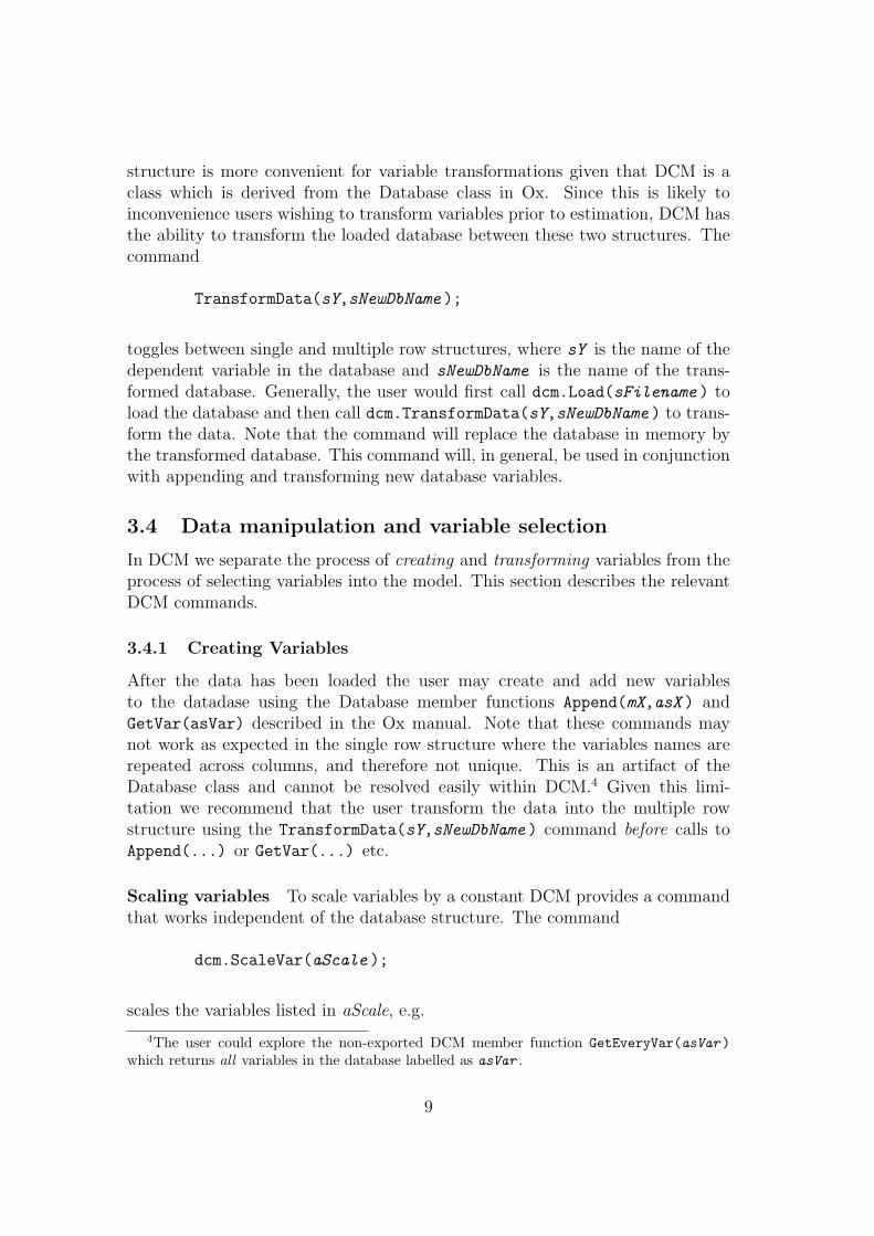
structure is more convenient for variable transformations given that DCM is aclass which is derived from the Database class in Ox. Since this is likely toinconvenience users wishing to transform variables prior to estimation, DCM hasthe ability to transform the loaded database between these two structures. Thecommand

TransformData(sY,sNewDbName );

toggles between single and multiple row structures, where sY is the name of thedependent variable in the database and sNewDbName is the name of the trans-formed database. Generally, the user would first call dcm.Load(sFilename ) toload the database and then call dcm.TransformData(sY,sNewDbName ) to trans-form the data. Note that the command will replace the database in memory bythe transformed database. This command will, in general, be used in conjunctionwith appending and transforming new database variables.

3.4 Data manipulation and variable selection

In DCM we separate the process of creating and transforming variables from theprocess of selecting variables into the model. This section describes the relevantDCM commands.

3.4.1 Creating Variables

After the data has been loaded the user may create and add new variablesto the datadase using the Database member functions Append(mX,asX ) andGetVar(asVar) described in the Ox manual. Note that these commands maynot work as expected in the single row structure where the variables names arerepeated across columns, and therefore not unique. This is an artifact of theDatabase class and cannot be resolved easily within DCM.4 Given this limi-tation we recommend that the user transform the data into the multiple rowstructure using the TransformData(sY,sNewDbName ) command before calls toAppend(...) or GetVar(...) etc.

Scaling variables To scale variables by a constant DCM provides a commandthat works independent of the database structure. The command

dcm.ScaleVar(aScale );

scales the variables listed in aScale, e.g.

4The user could explore the non-exported DCM member function GetEveryVar(asVar )which returns all variables in the database labelled as asVar .

9

dcm.ScaleVar(’’Var1’’,0.01,’’Var2’’,10);

will multiply Var1 by 0.01 and Var2 by 10 before estimation. The scaling occursinternally and the variables in the database are unchanged.

3.4.2 Selecting Variables

In the canonical form of a discrete choice model (see Eklof and Weeks (2004)),there are three distinct groups of variables: (1) the dependent variable, (2) indi-vidual characteristics, and (3) alternative attributes. The command

dcm.Select(iGroup,asVar );

selects the variables listed in asVar into group iGroup, where asVar follows thesyntax described in the Modelbase class5. The options for iGroup are presentedin Table 4.

Table 4: Select(iGroup,asVar ) options

iGroup DescriptionY VAR Dependent variable. Either an index or a dummy vari-

able.I VAR Individual characteristics.A VAR Alternative specific attributes.S VAR Choice Set Indicator.

Consider the case where the loaded database includes two attributes namedVar1 and Var2. The command

dcm.Select(A VAR,"Var1",0,0,"Var2",0,0);

selects database variables Var1 and Var2 into the group of alternative attributes.6

If the choice set varies across individuals, the command

dcm.Select(S VAR,asChoiceSetVar);

selects from the database the zero-one indicator variable asChoiceSetVar whichindicates for each individual whether a specific alternative is in the choice set.

5Note that the group X VAR is not used in DCM.6The 0’s relate to the potential use of lags in the model. However, as DCM v1.0 does not

support dynamic models these arguments must be set to 0.

10

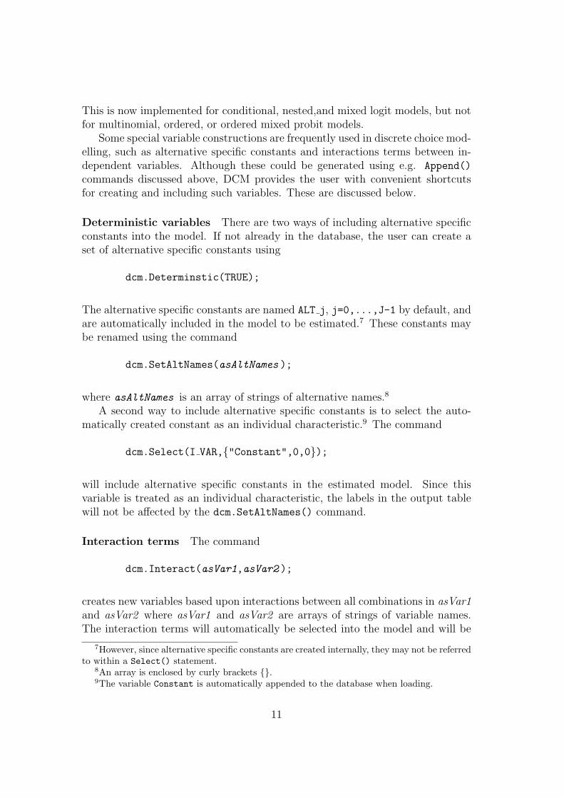
This is now implemented for conditional, nested,and mixed logit models, but notfor multinomial, ordered, or ordered mixed probit models.

Some special variable constructions are frequently used in discrete choice mod-elling, such as alternative specific constants and interactions terms between in-dependent variables. Although these could be generated using e.g. Append()

commands discussed above, DCM provides the user with convenient shortcutsfor creating and including such variables. These are discussed below.

Deterministic variables There are two ways of including alternative specificconstants into the model. If not already in the database, the user can create aset of alternative specific constants using

dcm.Determinstic(TRUE);

The alternative specific constants are named ALT j, j=0,...,J-1 by default, andare automatically included in the model to be estimated.7 These constants maybe renamed using the command

dcm.SetAltNames(asAltNames );

where asAltNames is an array of strings of alternative names.8

A second way to include alternative specific constants is to select the auto-matically created constant as an individual characteristic.9 The command

dcm.Select(I VAR,"Constant",0,0);

will include alternative specific constants in the estimated model. Since thisvariable is treated as an individual characteristic, the labels in the output tablewill not be affected by the dcm.SetAltNames() command.

Interaction terms The command

dcm.Interact(asVar1,asVar2 );

creates new variables based upon interactions between all combinations in asVar1and asVar2 where asVar1 and asVar2 are arrays of strings of variable names.The interaction terms will automatically be selected into the model and will be

7However, since alternative specific constants are created internally, they may not be referredto within a Select() statement.

8An array is enclosed by curly brackets .9The variable Constant is automatically appended to the database when loading.

11

named e.g. ”Var1*Var2”. Multiple calls to Interact(...) can be used tocreate ”blocks” of interaction terms. Note that dcm.Interact() does not checkfor linear dependence across created terms.

The command

dcm.RemoveInteract();

removes all interaction terms from the model.

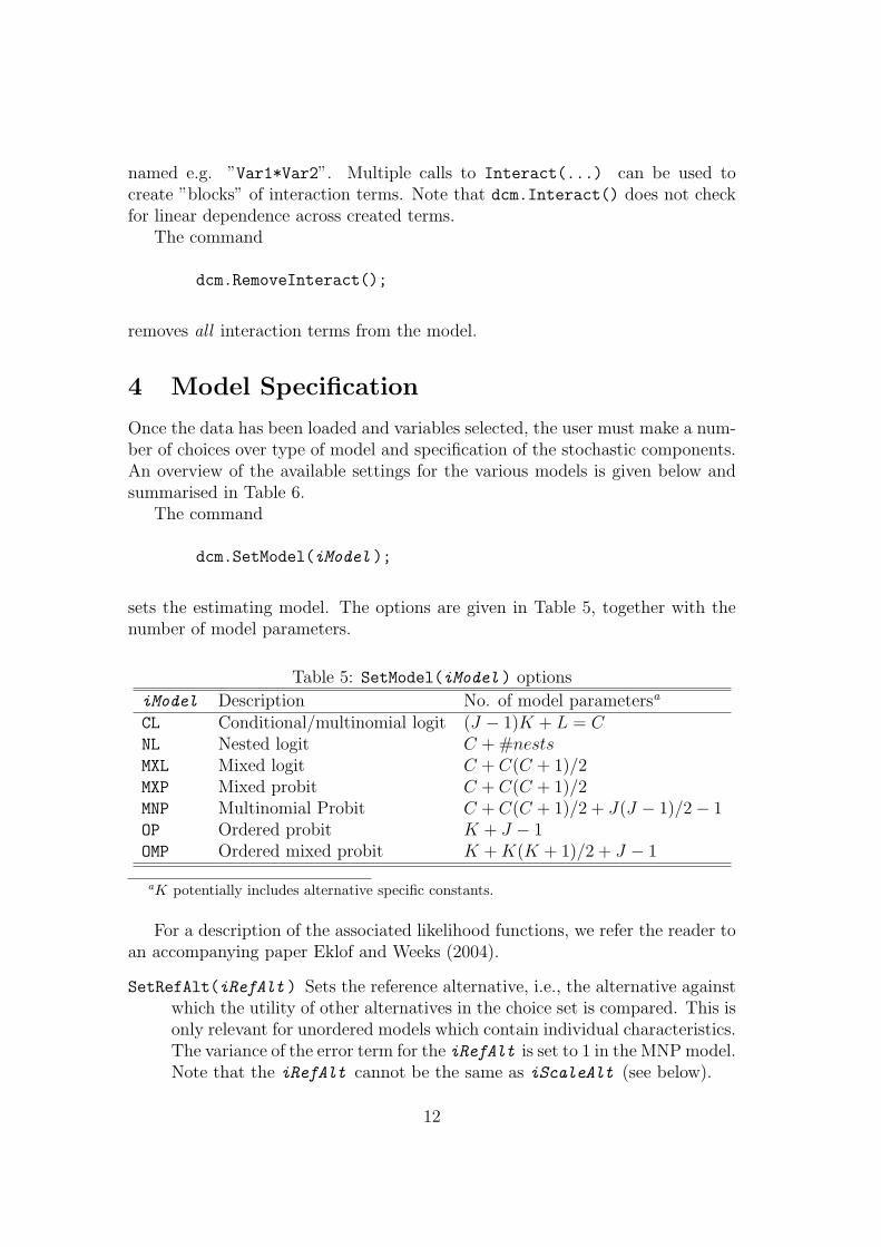
4 Model Specification

Once the data has been loaded and variables selected, the user must make a num-ber of choices over type of model and specification of the stochastic components.An overview of the available settings for the various models is given below andsummarised in Table 6.

The command

dcm.SetModel(iModel );

sets the estimating model. The options are given in Table 5, together with thenumber of model parameters.

Table 5: SetModel(iModel ) options

iModel Description No. of model parametersa

CL Conditional/multinomial logit (J − 1)K + L = CNL Nested logit C + #nestsMXL Mixed logit C + C(C + 1)/2MXP Mixed probit C + C(C + 1)/2MNP Multinomial Probit C + C(C + 1)/2 + J(J − 1)/2− 1OP Ordered probit K + J − 1OMP Ordered mixed probit K + K(K + 1)/2 + J − 1

aK potentially includes alternative specific constants.

For a description of the associated likelihood functions, we refer the reader toan accompanying paper Eklof and Weeks (2004).

SetRefAlt(iRefAlt ) Sets the reference alternative, i.e., the alternative againstwhich the utility of other alternatives in the choice set is compared. This isonly relevant for unordered models which contain individual characteristics.The variance of the error term for the iRefAlt is set to 1 in the MNP model.Note that the iRefAlt cannot be the same as iScaleAlt (see below).

12

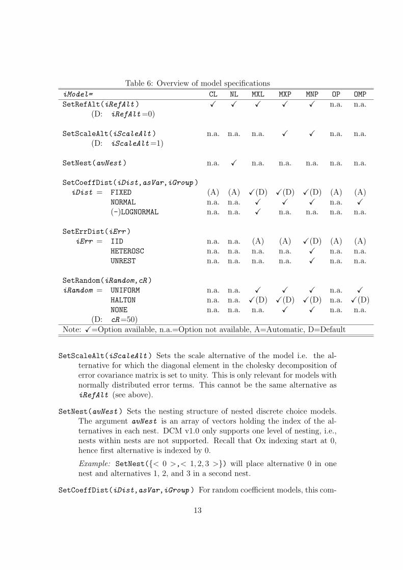
Table 6: Overview of model specifications

iModel= CL NL MXL MXP MNP OP OMP

SetRefAlt(iRefAlt ) X X X X X n.a. n.a.(D: iRefAlt=0)

SetScaleAlt(iScaleAlt ) n.a. n.a. n.a. X X n.a. n.a.(D: iScaleAlt=1)

SetNest(avNest ) n.a. X n.a. n.a. n.a. n.a. n.a.

SetCoeffDist(iDist,asVar,iGroup )

iDist = FIXED (A) (A) X(D) X(D) X(D) (A) (A)NORMAL n.a. n.a. X X X n.a. X(-)LOGNORMAL n.a. n.a. X n.a. n.a. n.a. n.a.

SetErrDist(iErr )

iErr = IID n.a. n.a. (A) (A) X(D) (A) (A)HETEROSC n.a. n.a. n.a. n.a. X n.a. n.a.UNREST n.a. n.a. n.a. n.a. X n.a. n.a.

SetRandom(iRandom,cR )

iRandom = UNIFORM n.a. n.a. X X X n.a. XHALTON n.a. n.a. X(D) X(D) X(D) n.a. X(D)NONE n.a. n.a. n.a. X X n.a. n.a.

(D: cR=50)Note: X=Option available, n.a.=Option not available, A=Automatic, D=Default

SetScaleAlt(iScaleAlt ) Sets the scale alternative of the model i.e. the al-ternative for which the diagonal element in the cholesky decomposition oferror covariance matrix is set to unity. This is only relevant for models withnormally distributed error terms. This cannot be the same alternative asiRefAlt (see above).

SetNest(avNest ) Sets the nesting structure of nested discrete choice models.The argument avNest is an array of vectors holding the index of the al-ternatives in each nest. DCM v1.0 only supports one level of nesting, i.e.,nests within nests are not supported. Recall that Ox indexing start at 0,hence first alternative is indexed by 0.

Example: SetNest(< 0 >,< 1, 2, 3 >) will place alternative 0 in onenest and alternatives 1, 2, and 3 in a second nest.

SetCoeffDist(iDist,asVar,iGroup ) For random coefficient models, this com-

13

Table 7: SetCoeffDist(iDist,asVar,iGroup ) options

iDist DescriptionFIXED Non-random coefficientNORMAL Normal distributed random coefficient(-)LOGNORMAL Log-normal distributed random coefficient

with positive (negative) support

mand sets the distribution of coefficients and the covariance structure. Thefirst argument sets the distribution of the parameters listed in the sec-ond argument. The (optional) iGroup argument allows for correlationacross random coefficients within groups (default iGroup=0). Coefficientsin group iGroup=0 are assumed uncorrelated, whereas as coefficients shar-ing the same iGroup> 0 number are allowed to correlate. This can be usedto allow for correlation across different types of distributions. iGroup cantake any integer value.

Example:dcm.SetCoeffDist(NORMAL,"Var1","Var2",1);dcm.SetCoeffDist(LOGNORMAL,"Var3","Var4",1);

sets coefficients associated with the variables V ar1 and V ar2 as distributedjoint normal and V ar3 and V ar4 to log-normal. Correlation within andacross normal and log-normal coefficients is allowed as they are all in thesame iGroup=1.

If the variable names listed in asVar do not exist among the model param-eters DCM terminates with an error.

The log-normal distribution has a positive support by default. To allow fornegative support, e.g. to model a negative price effect, insert a minus signbefore the LOGNORMAL specification.

Example: SetCoeffDist(-LOGNORMAL,"Var1","Var2",1);For asVar=-1 all coefficients in the model are assigned the distributionindicated by iDist and iGroup .

SetErrDist(iErr ) For the multinomial probit model, this command sets thestructure of the error covariance matrix. All available options in DCM willresult in an identified covariance matrix. Options are given in Table 8. SeeAppendix A.2 for a detailed description of the error covariance structure.

SetRandom(iRandom,cR ) Sets the type and number of random draws for mod-els that requires Monte Carlo integration techniques (MXL, MXP, MNP,and OMP). For low dimensional multiple index models with normally dis-tributed errors, the user can choose the option NONE and use the Ox nu-merical integration routines to estimate multivariate normal probabilities.

14

Table 8: SetErrDist(iErr ) options

iErr DescriptionIID Independently, identically distributed ran-

dom errorsHETEROSC Independent, heteroscedastic distributed

random errorsUNREST Unrestricted joint distributed random errors

(identified structure)

Table 9: SetRandom(iRandom,cR ) options

iRandom DescriptionUNIFORM Uniform pseudo random numbers generated

using Ox intrinsic commandsHALTON Equidistant sequence of numbersNONE Use standard numerical integration routines

4.1 Some comments on model specification

One of the principle distinctions between the mixed logit and multinomial probitmodel can be appreciated from Table 6. For example, consider the case where ananalyst is contemplating estimating either a mixed logit or multinomial probitmodel, and is interested in capturing estimates of random preference heterogene-ity. In the case of the MXL model the user will use SetCoeffDist() to makechoices as to whether individual mean coefficients are to be considered as fixed orrandom; and, if random, both the form of the mixing distribution and whetherrandom components are correlated. However, the use of the MNP model requiresboth this setting in conjunction with a specification on the residual error com-ponent using SetErrDist(). This follows from the fact that whereas the MXLmodel partitions the stochastic component into two additive parts - one het-eroscedastic and correlated over the choice set, and another which is i.i.d. type1 extreme value - the MNP model does not make such a distinction. Two otherobservations are worth making. First, one disadvantage of the MNP model is thatthe form of the mixing distribution is fixed and normal. In the current versionof DCM, a mixed logit model comes with two mixing distributions: normal andlog-normal. Second, if a MNP model is chosen and a user allows for free covari-ance parameters, identification restrictions are required. In contrast the mixedlogit model has at its core a kernel logit model, and therefore, identification isautomatic.

15

Table 10: SetAlgorithm(iAlgorithm ) options

iAlgorithm DescriptionBHHH Uses inverse of outer gradient product as es-

timate of the Hessian in a Newton type algo-rithm. Shipped with DCM

BFGS Intrinsic optimizer in OxNEWTON Intrinsic optimizer in Ox

Table 11: SetStdErr(iStdErr ) options

iStdErr DescriptionROBUST Use robust estimate of parameter covariance

matrixHESSIAN Use negative inverse of final Hessian of log-

likelihood functionOGP Use inverse of final outer gradient product of

log-likelihood function

5 Estimation

There are number of distinct commands which refer to estimation procedures.These are described below.

SetStartPar(vPar ) By default DCM uses conditional logit or ordered probitmodels to create parameter starting values for the more complicated models.This is overridden by this command.

Example: Consider the MXL model with 4 alternative specific constants, 1characteristic, and 1 attributes with a random coefficient. The command

SetStartPar(<1;2;3; // Alt. spec. constants

1;2;3; // characteristics

1; // attributes

0.5>); // std. err. of random coeff

would then set the starting values.

SetAlgorithm(iAlgorithm ) Toggless between available optimization routines.Options are given in Table 10

SetStdErr(iType ) Sets the type of estimated coefficient covariance matrix. Theoptions are described in Table 11.

Estimate() Estimates the specified model. Parameter estimates and covariancescan be extracted using e.g. dcm.GetPar() and dcm.GetCovar() commands.

16

6 Post-estimation

After successful estimation DCM provides a number of commands relating tooutput and testing. These are discussed below.

6.1 Output

OutputLaTeX(...), OutputLaTeX(aM0,...) Calling e.g. dcm.OutputLaTeX(aM0,aM1)will produce a LATEX formatted table with two columns of results for modelsM0 and M1. Parameters that are set to zero in a given model will appearas blanks. The arguments are optional. If no arguments are passed toOutputLaTeX(), DCM will use the most recent set of estimation results.

If arguments are submitted, they should appear as 5 element arrays con-sisting of: an q element array of names of estimated coefficients, a q × 1vector of estimates, a q × 1 vector of estimated standard errors, a scalarlog-likelihood value, and the number of observations. These arrays can beextracted using the member function dcm.GetAllResults(). For example,for model M0

decl aM0=dcm.GetAllResults()

6.2 Testing

TestRandCoeff(asVar ) Tests for unobserved heterogeneity in coefficients. Thetest is operationalized by adding a number of artificial variables constructedfrom a previous CL estimation, and then re-estimating the model. The testis based upon a set of exclusion restrictions, with a chi-square distribution.asVar is an array of variable names indicating coefficients will be testedfor heterogeneity. Setting asVar=-1 test all coefficients.

7 Examples

In what follows we demonstrate the use of DCM with reference to a number ofexamples.

7.1 Conditional, Nested, and Mixed logit models

Following earlier work by Daganzo (1979) and McFadden (1977), the transportmode choice problem has continued to figure prominently in both reflecting andpromoting developments in discrete choice methodology. In recognition of thisfact, we examine a well known modal choice dataset recording the inter-citytravel choices between Melbourne, Canberra and Sydney. There are a total of

17

Table 12: Example A: Conditional logit with post-estimation testing

1 #include <oxstd.h>

2 #include "packages\dcm\dcm.ox" // Include DCM package

3

4 main()

5

6 decl dcm = new DCM(); // Create a DCM object

7 dcm.Load("Greene.xls"); // Load database

8 dcm.Deterministic(TRUE); // Append alt. spec. constants

9 dcm.SetAltNames("air","train","bus","car"); // Set new alt. names

10 dcm.Select(Y_VAR,"Mode",0,0); // Select dependent variable

11 dcm.Select(A_VAR,"GC",0,0,"Ttme",0,0); // Select independent variables

12 dcm.Interact("air","Hinc"); // Append and select interactions

13 dcm.SetRefAlt("car"); // Set reference alternative

14 dcm.SetAlgorithm(BFGS); // Use BFGS optimizer

15 dcm.Estimate(); // Estimate the model

16 dcm.TestRandCoeff(-1); // Test all coefficients

17 dcm.TestRandCoeff("air","train","bus"); // Test a subset of coefficients

18

210 observations of non-business travellers faced with the choice between plane,train, bus, and car.10 This dataset has been used extensively with examplesincluding Greene (2002), Louviere, Hensher, and Swait (2000), and Ben-Akiva,Bolduc, and Walker (2001). The covariates included are terminal waiting time(Ttme), in-vehicle cost (Invc), in-vehicle time (Invt), generalized costs (GC)calculated from Invt, Invc, and a measure of wage rates, and household income(Hinc) interacted with the ”air” alternative. The estimated model is

Uj = αj + β1GCj + β2Ttmej + β3(Hinc ∗ airj) + εj,

where αj is an alternative specific constant and airj is a alternative specificdummy.

In table 12 we present the code which allows the user to estimate a conditionallogit model, followed by a test for random preference heterogeneity.

Fragments from the output produced by the code is presented in Table ??.An ellipse (. . . ) indicates that some output has been omitted.

In examining the output we first note that DCM summarises the principalfeatures of the data by indicating the number of individuals N , time periods T (ifT > 1), and alternatives J . For unbalanced panel DCM will report the minimumand maximum number of time periods and the frequency of the observed periods.DCM also reports the chosen reference and scale alternatives where appropriate.Following this, DCM reports the estimated coefficients and their standard errors,

10Note that the dataset is actually choice-based, with undersampling of the more popularmode, car. In order to obtain consistent estimates a weighted exogenous sample maximumlikelihood estimator (WESML) should be used. However, we do not do this, since our primaryobjective is to compare our estimates with those in Greene (2002) and Louviere, Hensher, andSwait (2000).

18

Table 13: Example A: Conditional logit, output fragments

1 ---- DCM: Conditional Logit ----

2 The estimation sample is: 1 (1) - 210 (4)

3 The dependent variable is: Mode (Greene.xls)

4 Data structure : NTJ x K+L+1 with

5 N = 210

6 J = 4

7 Reference alternative: car

8

9 Coefficient Std.Error t-value t-prob

10 -- ASC --

11 air 5.20744 0.9789 5.32 0.000

12 train 3.86904 0.5175 7.48 0.000

13 bus 3.16319 0.5463 5.79 0.000

14 -- Attributes --

15 GC -0.0155015 0.004945 -3.13 0.002

16 Ttme -0.0961248 0.01506 -6.38 0.000

17 -- Interactions --

18 air*Hinc 0.0130870 0.009264 1.41 0.159

19

20 NOTE: Robust standard errors.

21

22 log-likelihood -199.128369

23 no. of observations 210 no. of parameters 6

24 AIC.T 410.256737 AIC 1.95360351

25 Time to convergence: 0.04 (hh:mm:ss.hs, excluding time for covariance.)

26 BFGS using analytical derivatives (eps1=0.0001; eps2=0.005):

27 Strong convergence

28 Used starting values:

29 0.00000 0.00000 0.00000 0.00000 0.00000 0.00000

30 ...

31 Test for excluding:

32 ...

33 Subset Chi^2(6) = 74.9196 [0.0000] **

34 ...

35 Test for excluding:

36 ...

37 Subset Chi^2(3) = 55.2356 [0.0000] **

19

Table 14: Example B: Nested logit with variable transformations


2 #include "packages\dcm\dcm.ox"

3

4 main()

5

6 decl dcm = new DCM(); // Create DCM object

7 dcm.Load("Greene.xls"); // Load database

8 // Append alt. spec. constants

9 dcm.Append(ones(210,1)**unit(4),"air","train","bus","car");

10 // Append interaction term

11 dcm.Append(dcm.GetVar("air").*dcm.GetVar("Hinc"),"air*Hinc");

12 dcm.Select(Y_VAR,"Mode",0,0); // Select dependent variable

13 // Select independent variables

14 dcm.Select(A_VAR,"air",0,0,"train",0,0,"bus",0,0,

15 "GC",0,0,"Ttme",0,0,"air*Hinc",0,0);

16 dcm.SetRefAlt(3); // Set reference alternative

17 dcm.SetModel(NL); // Set model

18 dcm.SetNest(<0>,<1,2,3>); // Set nesting structure

19 dcm.SetAlgorithm(BFGS); // Set algorithm

20 dcm.Estimate(); // Estimate model

21

subdivided into the variable categories (alternative specific constants, attributes,characteristics, etc.). Below this section standard deviations and correlationsof random coefficients and error terms are reported, again where appropriate.Finally, DCM reports the value of the maximised log-likelihood and the startingvalues.

The TestRandCoeff(asVar ) commands produces a similar sets of outputsgiven that this test involves re-estimating the model with artificial variables (which are denoted by the prefix "ART "). In Table 13 we present the specific setof outputs from these tests, which are based upon exclusion restrictions for theartificial variables. Test statistics and corresponding p-values are also provided.

In Table 14 the code for the Nested logit model is presented. We assumethat the modes can be partitioned into ”fly” and ”ground” nests, such that ”air”(alternative 1 is indexed by 0) is in one nest and ”train”, ”bus”, and ”car” (al-ternatives 2, 3, and 4 are indexed as 1,2, and 3, respectively) is in a second. Notethat even though the first nest contains a single alternative, the argument mustbe a vector rather than a scalar. Fragments of the output are presented in Table15. To illustrate the use of the Database commands Append() and GetVar(), weconstruct alternative specific constants and interaction terms manually. See theOx manual for syntax.

The additional information printed for the Nested logit model is the nestingstructure and the set of variables that are constant or varying within nests. Thisinformation is given in the first panel. The estimates’ panel now includes theestimates of the coefficients of the ”inclusive values”.

The last model estimated in this subsection is the Mixed logit model. In

20

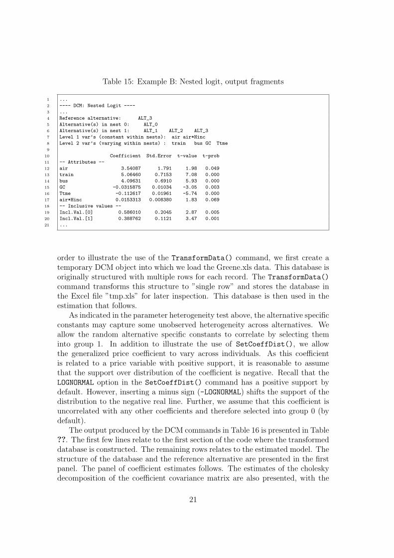
Table 15: Example B: Nested logit, output fragments

1 ...

2 ---- DCM: Nested Logit ----

3 ...

4 Reference alternative: ALT_3

5 Alternative(s) in nest 0: ALT_0

6 Alternative(s) in nest 1: ALT_1 ALT_2 ALT_3

7 Level 1 var’s (constant within nests): air air*Hinc

8 Level 2 var’s (varying within nests) : train bus GC Ttme

9


11 -- Attributes --

12 air 3.54087 1.791 1.98 0.049

13 train 5.06460 0.7153 7.08 0.000

14 bus 4.09631 0.6910 5.93 0.000

15 GC -0.0315875 0.01034 -3.05 0.003

16 Ttme -0.112617 0.01961 -5.74 0.000

17 air*Hinc 0.0153313 0.008380 1.83 0.069

18 -- Inclusive values --

19 Incl.Val.[0] 0.586010 0.2045 2.87 0.005

20 Incl.Val.[1] 0.388762 0.1121 3.47 0.001

21 ...

order to illustrate the use of the TransformData() command, we first create atemporary DCM object into which we load the Greene.xls data. This database isoriginally structured with multiple rows for each record. The TransformData()

command transforms this structure to ”single row” and stores the database inthe Excel file ”tmp.xls” for later inspection. This database is then used in theestimation that follows.

As indicated in the parameter heterogeneity test above, the alternative specificconstants may capture some unobserved heterogeneity across alternatives. Weallow the random alternative specific constants to correlate by selecting theminto group 1. In addition to illustrate the use of SetCoeffDist(), we allowthe generalized price coefficient to vary across individuals. As this coefficientis related to a price variable with positive support, it is reasonable to assumethat the support over distribution of the coefficient is negative. Recall that theLOGNORMAL option in the SetCoeffDist() command has a positive support bydefault. However, inserting a minus sign (-LOGNORMAL) shifts the support of thedistribution to the negative real line. Further, we assume that this coefficient isuncorrelated with any other coefficients and therefore selected into group 0 (bydefault).

The output produced by the DCM commands in Table 16 is presented in Table??. The first few lines relate to the first section of the code where the transformeddatabase is constructed. The remaining rows relates to the estimated model. Thestructure of the database and the reference alternative are presented in the firstpanel. The panel of coefficient estimates follows. The estimates of the choleskydecomposition of the coefficient covariance matrix are also presented, with the

21

Table 16: Example C: Mixed logit with ”single row” data structure



3

4 main()

5

6 // Transform "multiple row structure" to "single row structure"

7 decl dcm0 = new DCM(); // Create DCM object

8 dcm0.Load("Greene.xls"); // Load original database

9 dcm0.TransformData("Mode","tmp.xls"); // Transform and save database

10 delete dcm0; // Delete this object

11

12 decl dcm = new DCM();

13 dcm.Load("tmp.xls"); // Load temporary *transformed* database

14 dcm.Deterministic(TRUE);

15 dcm.SetAltNames("air","train","bus","car");

16 dcm.Select(Y_VAR,"Mode",0,0);

17 dcm.Select(A_VAR,"GC",0,0,"Ttme",0,0);

18 dcm.Interact("air","Hinc");

19 dcm.SetRefAlt("car");

20 dcm.SetModel(MXL); // Set model to MXL

21 dcm.SetCoeffDist(NORMAL,"air","train","bus",1); // Set distr. of coeff’s

22 dcm.SetCoeffDist(-LOGNORMAL,"GC"); // Use negative support for price coeff’s

23 dcm.SetRandom(HALTON,100); // Set type and no. of random draws

24 dcm.SetAlgorithm(BFGS);

25 dcm.Estimate();

26

numbers in square brackets indicating the position in the cholesky matrix. Be-low the estimates, DCM reports the standard errors and the correlations of therandom coefficients.

7.2 Multinomial probit models

To demonstrate the specification and estimation of multinomial probit modelswe use the trinomial discrete choice model of the labour force status of marriedwomen in the UK as considered by Duncan and Weeks (1998). The model isdiscrete in that they allow for three states: non-workers supplying zero hours ofwork; part-time workers whose weekly supply is between 0 and 30 hours; and full-time workers supplying more than 30 hours. The data consist of a random sampleof married women drawn from the 1993 Family Expenditure Survey (FES).

Across all specifications we condition our labour supply model on wage rates,11

and the following socio-demographic characteristics ; age of the woman, dummiesfor children in the age groups 0-2, 3-4, 5-10, and above 11, number of children,level of formal education and marital status (whether married or cohabiting).

11Since wage rates are not observed in the FES for those not in employment, we base our sim-ulations on wage rate estimates derived from an appropriately corrected reduced form equation.See Duncan and Weeks for further details.

22

Table 17: Example C: Mixed logit, output fragments

1 ...

2 DCM package version 1.00, object created on 19-05-2004

3 ** NOTE: Transforming multiple to single row structure

4 ...

5 ---- DCM: Mixed Logit ----


7 The dependent variable is: Mode (tmp.xls)

8 Data structure : Single row per record with

9 N = 210

10 J = 4

11 Pseudo random draws: HALTON (R=100)

12 Reference alternative: car

13


15 -- ASC --

16 (1) air 4.33782 2.810 1.54 0.124

17 (2) train 5.49412 3.032 1.81 0.071

18 (3) bus 4.44471 2.555 1.74 0.083

19 -- Attributes --

20 (4) GC -3.36821 1.029 -3.27 0.001

21 (5) Ttme -0.115666 0.03849 -3.00 0.003

22 -- Interactions --

23 (6) air*Hinc 0.0466768 0.07750 0.602 0.548

24 -- Cholesky elements of Cov[coeff] --

25 C(Par)[1,1] 4.06479 5.805 0.700 0.485

26 C(Par)[1,2] 0.724140 1.533 0.472 0.637

27 C(Par)[1,3] 0.438704 0.9484 0.463 0.644

28 C(Par)[2,2] -0.532236 4.143 -0.128 0.898

29 C(Par)[2,3] -0.345838 2.548 -0.136 0.892

30 C(Par)[3,3] -0.00261691 0.05693 -0.0460 0.963

31 C(Par)[4,4] 0.00554049 0.1620 0.0342 0.973

32

33 ** NOTE: Robust standard errors.

34 ** NOTE: Mean parameters for log-normal distr. coefficients are

35 calculated as E[ln(beta)] (E[ln(-beta)] for neg. log-norm.).

36

37 Random parameters:

38 Parameter Std. dev. Correlation matrix (*=fixed, not estimated)

39 (1) air 4.063 1.000

40 (2) train 0.898 0.807 1.000

41 (3) bus 0.558 0.786 0.999 1.000

42 (4) GC 0.000 0* 0* 0* 1.000

43 ...

23

We also include a single attribute variable, net incomes at various hours levels.To generate state-specific net incomes as condition variables for the structuraldiscrete choice models, we simulate tax liabilities and benefit receipts and totalnet incomes at 0, 20 and 40 hours for each individual in our sample.12 Finally,to allow for age dependent income effect, we interact net income and age. Ourdependent variable is a three-state variable which distinguishes non-participants(category 0), part-time workers between 1 and 30 hours (category 1) and full-timers working in excess of 30 hours (category 2). The reference alternative isthe non-participation category. In reading the economic significance of the pa-rameter estimates, a negative coefficient represents a decrease in the likelihood ofworking either part-time or full-time relative to not working. Which comparisonis appropriate is identified for each parameter estimate in the table.

We consider a number of alternative model specifications by focusing uponthe stochastic component of choice. These are: the MNL model (Model 1), aMNP with heteroscedastic error terms (Model 2), and a MNP with one randomcoefficient and IID errors (Model 3).

The DCM commands for estimating these models are presented in Table 18.13

We also illustrate a number of additional features of DCM and Modelbase, suchas extracting estimates and producing LaTeX formatted tables after estimatingmultiple models. Some of these features require knowledge of the Ox program-ming. We refer the interested user to the Ox manual.

Noteb that in the example code we call the member function GetAllResults().This command returns an array of results which we will use to tabulate param-eter names, estimates, and standard errors, together with the final loglikelihoodvalue and the number of observations. These are stored in an array which willlater be used calling the OutputLaTeX(...) command. In Table 19 we presentthe actual table produced by the code. ”*” and ”**” denote significance at the10 and 1 per cent level.

8 Monte Carlo experiments using Generate()

In addition to estimating discrete choice models based upon observed data, DCMallows the user the option to generate discrete choice data. This may be accom-

12The wage equation is identified from the inclusion of demand-side (quarterly unemploy-ment) and regional characteristics (vacancies and redundancies by region) as well as socio-demographic characteristics (quadratics and interactions between age, partners’s age and ed-ucation; age and number of children). Estimates are available from the authors on request.A problem with this approach is that it becomes difficult to correct the standard errors inthe structural model for the inclusion of the generated wage rate term, since the simulatednet income terms also depend (non-linearly) on the wage rate used. In the structural models,therefore, the standard errors remain uncorrected.

13See Duncan and Weeks (1998) for a discussion of parameter estimates and the applicationof both nested and non-nested tests across models.

24

Table 18: Example D: Conditional Logit and Multinomial probit models


2 #include "packages\\dcm\\dcm.ox" //

3 Include DCM package

4

5 main()

6 decl dcm = new DCM();

7 dcm.Load("Married4.xls");

8 dcm.Select(Y_VAR,"REFPRED",0,0); // Dependent variable

9 // Individual characteristics

10 dcm.Select(I_VAR,"DKID02",0,0,"DKID34",0,0,"DKID510",0,0,

11 "DKID110",0,0,"TOT_KIDS",0,0,"AGE",0,0,

12 "EDGT16",0,0,"COHAB",0,0,"LNWFIT",0,0);

13 dcm.Select(A_VAR,"INC",0,0); // Alternative attributes

14 dcm.ScaleVar("INC",0.01); // Multiply INC by 0.01 before estimation

15 dcm.SetAlgorithm(BFGS);

16

17 // Model 1: Conditional logit

18 dcm.SetModel(CL);

19 dcm.Estimate();

20 decl aM1 = dcm.GetAllResults(); // Store relevant est. results in array

21

22 // Model 2: No random coefficients, heteroscedastic error covariance struct.

23 dcm.SetModel(MNP);

24 dcm.SetRandom(HALTON,50);

25 dcm.SetErrDist(HETEROSC);

26 dcm.Estimate();

27 decl aM2 = dcm.GetAllResults();

28

29 // Model 3: Normal distr. inc. coefficient, IID error covariance structure

30 dcm.SetCoeffDist(NORMAL,"INC"); // Normal distr. inc. coefficient

31 dcm.SetErrDist(IID);

32 dcm.SetStartPar(dcm.GetPar()[:18]| // Mean coefficients

33 1); // standard dev. of random coeff.

34 dcm.SetRandom(HALTON,50);

35 dcm.Estimate();

36 decl aM3 = dcm.GetAllResults();

37

38 // Print all results to one LaTeX table

39 dcm.OutputLaTeX(aM1,aM2,aM3); // Print results from model 1-3 in table

40

25

Table 19: Example D: Multinomial models. Automated LaTeX output

Model 1 Model 2 Model 3(1) DKID02 1/0 -4.168* -2.753 -2.449

(1.865) (1.931) (1.828)(2) DKID02 2/0 -23.813** -19.122** -21.272**

(3.716) (5.932) (3.391)(3) DKID34 1/0 14.807** 12.780** 13.388**

(2.254) (2.150) (2.428)(4) DKID34 2/0 -27.924** -22.594** -24.841**

(4.306) (7.205) (3.741)(5) DKID510 1/0 34.780** 29.465** 30.642**

(3.484) (5.680) (4.222)(6) DKID510 2/0 0.317 1.065 -0.518

(3.339) (2.799) (3.040)(7) DKID110 1/0 29.620** 24.876** 27.244**

(3.230) (4.402) (4.272)(8) DKID110 2/0 4.764 4.538* 4.687

(3.036) (2.283) (3.096)(9) TOT KIDS 1/0 -7.730** -6.470** -6.533**

(0.887) (1.556) (0.879)(10) TOT KIDS 2/0 -7.326** -6.139** -6.333**

(0.918) (1.509) (0.984)(11) AGE 1/0 3.088* 2.832* 3.299*

(1.801) (1.323) (1.713)(12) AGE 2/0 -20.998** -17.010** -18.874**

(3.115) (5.290) (2.982)(13) EDGT16 1/0 -0.059 0.128 -0.080

(0.636) (0.530) (0.527)(14) EDGT16 2/0 -0.004 0.154 -0.072

(0.639) (0.561) (0.539)(15) COHAB 1/0 -9.873** -8.254** -8.164**

(1.931) (2.750) (1.787)(16) COHAB 2/0 4.882** 4.138** 4.784**

(1.543) (1.405) (1.593)(17) LNWFIT 1/0 8.208** 6.599** 6.421**

(1.757) (2.363) (1.534)(18) LNWFIT 2/0 19.701** 15.956** 17.209**

(2.472) (4.402) (2.399)(19) INC 4.281** 3.566** 3.608**

(0.455) (0.798) (0.469)C(Err)[2,2] – 1.308* –

(0.523)C(Par)[19,19] – – 0.503*

(0.242)Loglik. -129.2 -130.622 -127.488Obs. 1520 1520 1520

26

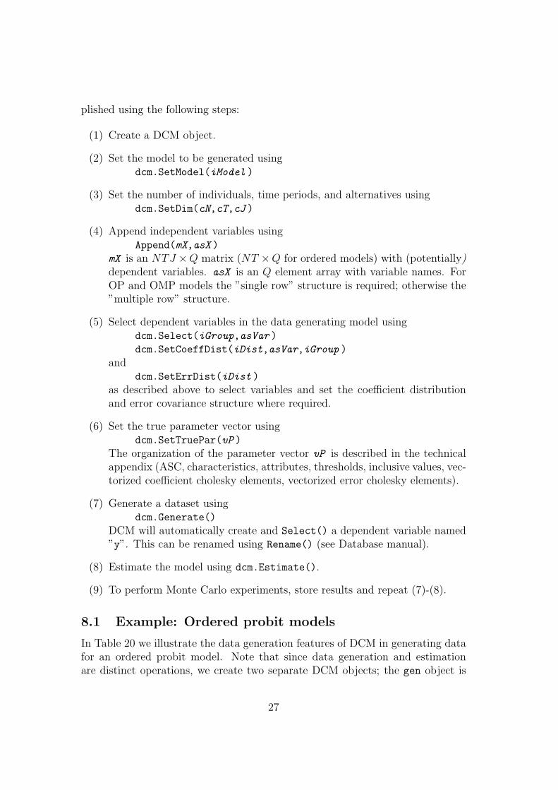
plished using the following steps:

(1) Create a DCM object.

(2) Set the model to be generated usingdcm.SetModel(iModel )

(3) Set the number of individuals, time periods, and alternatives usingdcm.SetDim(cN,cT,cJ )

(4) Append independent variables usingAppend(mX,asX )

mX is an NTJ ×Q matrix (NT ×Q for ordered models) with (potentially)dependent variables. asX is an Q element array with variable names. ForOP and OMP models the ”single row” structure is required; otherwise the”multiple row” structure.

(5) Select dependent variables in the data generating model usingdcm.Select(iGroup,asVar )

dcm.SetCoeffDist(iDist,asVar,iGroup )

anddcm.SetErrDist(iDist )

as described above to select variables and set the coefficient distributionand error covariance structure where required.

(6) Set the true parameter vector usingdcm.SetTruePar(vP )

The organization of the parameter vector vP is described in the technicalappendix (ASC, characteristics, attributes, thresholds, inclusive values, vec-torized coefficient cholesky elements, vectorized error cholesky elements).

(7) Generate a dataset usingdcm.Generate()

DCM will automatically create and Select() a dependent variable named”y”. This can be renamed using Rename() (see Database manual).

(8) Estimate the model using dcm.Estimate().

(9) To perform Monte Carlo experiments, store results and repeat (7)-(8).

8.1 Example: Ordered probit models

In Table 20 we illustrate the data generation features of DCM in generating datafor an ordered probit model. Note that since data generation and estimationare distinct operations, we create two separate DCM objects; the gen object is

27

Table 20: Example E: Ordered probit and simulation


2 #include "packages\\dcm\\dcm.ox"

3

4 main()

5

6 decl gen = new DCM(); // (1) Create DCM object

7 gen.SetModel(OP); // (2) Set model to simulate

8 gen.SetDim(1000,1,4); // (3) Set dimension of database

9 gen.Append(rann(1000,2),"x1","x2"); // (4) Append variables

10 gen.Select(I_VAR,"x1",0,0,"x2",0,0); // (5) Select variables to true model

11 gen.SetTruePar(<1;1;-1;0;1>); // (6) Set true parameter vector

12 gen.Generate(); // (7) Generate dependent variable "y"

13 gen.SaveXls("sim.xls"); // Save database in Excel

14 delete gen; // Delete object

15

16 decl dcm = new DCM(); // Create new DCM object

17 dcm.Load("sim.xls"); // Load database

18 dcm.Select(Y_VAR,"y",0,0); // Select dependent variable

19 dcm.Select(I_VAR,"x1",0,0,"x2",0,0); // Select independent variables

20 dcm.SetModel(OP); // Set model

21 dcm.Estimate(); // (8) Estimate

22 dcm.OutputLaTeX(); // Print LaTeX table

23

used for generating a dataset, and the dcm object is used as previously described.Output is written in a LaTeX table format.

Table ?? presents fragments of the output. In the estimate section thereis a new label indicating estimates of thresholds. We note that the orderedprobit model is identified with respect to location by dropping the constant andestimating all J − 1 thresholds.

In the last example we demonstrate how to utilise DCM in a small MonteCarlo experiment, generating and estimating an ordered mixed probit model. Inthis example, the data generation and estimation is conducted within the sameobject. Note that we do not need to Select() variables in the estimation stepas this is automatically done in the generation step. We report the generateddistributions of the estimated coefficients and thresholds.14

9 DCM in OxPack for GiveWin

In this section we describe the OxPack implementation of DCM. In order touse the OxPack implementation the user must have an OxProfessional licenseproperly installed. Before DCM can be used within OxPack the package mustbe added to the list of available packages. To do this start the OxPack modulein GiveWin and use the ”Package-Add/Remove Package...” menu to locate and

14If using DCM via GiveWin, the figure should be produced by GiveWin, otherwise the userneed to locate and open the ”OMPMC.eps” file to inspect the graphical results.

28

Table 21: Example E: Ordered probit, output fragments

1 ---- DCM: Ordered Probit ----


3 The dependent variable is: y (sim.xls)

4 Data structure : NT x (J or 1)K+JL+(J or 1) with

5 N = 1000

6 J = 4

7


9 -- Characteristics --

10 x1 0.950045 0.04647 20.4 0.000

11 x2 0.998723 0.04559 21.9 0.000

12 -- Thresholds --

13 alpha1 -1.03566 0.05612 -18.5 0.000

14 alpha2 0.0483520 0.04828 1.00 0.317

15 alpha3 0.974644 0.05542 17.6 0.000

16 ...

Table 22: Example E: Ordered mixed probit and Monte Carlo experiment



3

4 main()

5

6 decl mc = new DCM(); // Create DCM object

7 mc.SetModel(OMP); // Set model to simulate

8 mc.SetDim(1000,1,4); // Set dimension of database

9 mc.Append(rann(1000,2),"x1","x2"); // Append variables

10 mc.Select(I_VAR,"x1",0,0,"x2",0,0); // Select variables to true model

11 mc.SetCoeffDist(NORMAL,"x1");

12 mc.SetTruePar(<1;1;-1;0;1;0.5>); // Set true parameter vector

13 decl mP = <>;

14 mc.SetPrint(FALSE); // No print-outs

15 for (decl r=0;r<100;++r) // Start MC replications

16 println("Replication ",r);

17 mc.Generate(); // Generate dependent variable "y"

18 mc.Estimate(); // Estimate model.

19 if (mc.GetResult()==MAX_CONV) // Store results if convergence

20 mP ~= mc.GetFreePar();

21

22 decl asLegend=;

23 for (decl p=0;p<mc.GetFreeParCount();++p)

24 asLegend ~= sprint(mc.GetFreeParNames()[p],"=",mc.GetTruePar()[p]);

25 DrawDensity(0,mP,asLegend,1,0,0);

26 ShowDrawWindow();

27 SaveDrawWindow("OMPMC.eps");

28 delete mc;

29

29

Figure 1: Example F: Ordered mixed probit and Monte Carlo generated distri-butions

0.5 1.0 1.5 2.0 2.5

0.5

1.0

1.5

Density(1) x1=1

0.50 0.75 1.00 1.25 1.50 1.75

0.5

1.0

1.5

Density(2) x2=1

−2.0 −1.5 −1.0 −0.5

0.5

1.0

1.5

Densityalpha1=−1

−0.50 −0.25 0.00 0.25 0.50 0.75

1

2

Densityalpha2=0

0.5 1.0 1.5 2.0

0.5

1.0

1.5

Densityalpha3=1

−1.0 −0.5 0.0 0.5 1.0 1.5 2.0 2.5

0.25

0.50

0.75

DensityC(Par)[1,1]=0.5

select the DCM.ox file. Users may now choose DCM from the ”Packages” menuin OxPack. Assuming that a proper database has been loaded, the user may nowestimate any of the available models in DCM.

9.1 Limitations in OxPack implementation

1. The OxPack implementation of DCM can only be used with ”multiple row”data structures

2. Variable constructions, such as Interact(), must be performed using thecalculator or algebra code in GiveWin.

3. Output cannot be translated to LaTeX code.

4. Using the simulation capabilities only standard normal distributed covari-ates can be considered.

5. Online help is not available.

In the following sub-sections we describe the dialogs which relate to the multi-nomial probit model. In focussing upon this example, we are able to cover a rangeof specification issues that apply to other models within DCM.

30

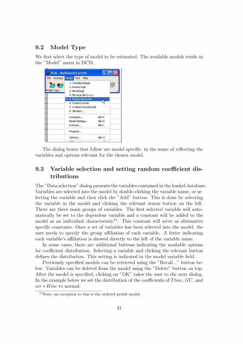
9.2 Model Type

We first select the type of model to be estimated. The available models reside inthe ”Model” menu in DCM.

The dialog boxes that follow are model specific, in the sense of reflecting thevariables and options relevant for the chosen model.

9.3 Variable selection and setting random coefficient dis-tributions

The ”Data selection” dialog presents the variables contained in the loaded database.Variables are selected into the model by double-clicking the variable name, or se-lecting the variable and then click the ”Add” button. This is done by selectingthe variable in the model and clicking the relevant status button on the left.There are three main groups of variables. The first selected variable will auto-matically be set to the dependent variable and a constant will be added to themodel as an individual characteristic15. This constant will serve as alternativespecific constants. Once a set of variables has been selected into the model, theuser needs to specify the group affiliation of each variable. A letter indicatingeach variable’s affiliation is showed directly to the left of the variable name.

In some cases, there are additional buttons indicating the available optionsfor coefficient distribution. Selecting a variable and clicking the relevant buttondefines the distribution. This setting is indicated in the model variable field.

Previously specified models can be retrieved using the ”Recall...” button be-low. Variables can be deleted from the model using the ”Delete” button on top.After the model is specified, clicking on ”OK” takes the user to the next dialog.In the example below we set the distribution of the coefficients of Ttme, GC, andair ∗Hinc to normal.

15Note: an exception to this is the ordered probit model.

31

9.4 Estimation and model options

In the ”Estimate Model” dialog the user can set the optimization algorithm andother model options. To use the default settings press ”OK” and the model willbe estimated.

In the ”Model Options” dialog, the user can set model specific options. Forexample, for the conditional/multinomial logit model there are two available op-tions; the type of covariance estimator and the reference alternative. Clickingon the radio buttons sets the covariance estimator. The reference alternative isset by choosing a specific alternative from the list provided. In this dialog theuser can specify the correlation structure of the random coefficients. The coef-ficients which are marked as random in the Model selection dialog are listed inthe Options dialog where the user can set the relevant group for each coefficient.Coefficients listed in the same group may correlated with the exception of the

32

special group 0 which is assumed to include only uncorrelated coefficients.Related to the optimization procedure, a number of settings control the maxi-

mum number of iterations, type of printout during optimization, and convergencecriteria. After the options have been set, clicking on ”OK” takes the user backto the ”Estimate Model” dialog.

After the model has been estimated, the output will appear in the GiveWinoutput window. The user may now re-estimate the model using a different set ofvariables and/or options.

10 Notes, remarks, and history

10.1 Bug reports and version history

Version 1.0, released June 2004 • First version. Substantial amount ofbug fixes and developments since beta version. Not listed.

10.2 Future plans

A Technical appendix

A.1 Inference on data structure

DCM infers the form of data structure from the selected dependent. The mainissue is to determine whether records in the database include single or multiplerows. To do this DCM initially checks for multiple occurrences of the dependentvariable in the set of variable names in the database. DCM then checks thevalues of the dependent variable and infers the data structure, the number of

33

alternatives, individuals and time periods. In what follows, we present the generaloutline of this procedure.

1. Dependent Variable as a single column: If there is a single variable inthe database named as the dependent variable DCM will continue to checkif the maximum value of the dependent variable is 1 or larger.

Maximum value is 1: If the maximum value is 1 we may have the casethat the data represents a binomial model where the dependent vari-able is recorded as a 1 or 0. This is a common but special case whereeach row in the data corresponds to one record, i.e., a ”single row”data structure. In order to differentiate between this instance and onewhere the dependent variable is an indicator but records span mul-tiple rows, DCM analyzes the ratio between the number of rows inthe dataset and the number of 1’s in the dependent variable. If thenumber of rows is a multiple of the number of 1’s is zero, this indicatesthat the data is structured with multiple rows per record, otherwise itis structured as ”single row”.16

If the structure corresponds to the ”multiple row” case, the numberof alternatives J is derived as the number of rows in the dataset di-vided by the number of 1’s in the dependent variable. The number ofindividuals N is then derived as the the number of rows in the data di-vided by the number of time periods and alternatives (if cross-sectionor balanced panel); or the number of unique values in the individualID variable set by SetId(sVar ) (if unbalanced panel). If the struc-ture is ”single row”, the number of alternatives J is 2, the number ofindividuals N is the number of rows divided by the number of timeperiods or the number of unique values in the individual ID variable.

Maximum value is greater than 1: If the maximum value of the de-pendent variable is greater than 1, it should not be a indicator. DCMwill then infer that the dependent variable provides the index of thepreferred choice and that the data structure is of the ”single row”type. DCM also checks if the indexing starts at 0 or 1, and adjusts theindexing accordingly. The number of alternatives J is determined bythe difference between the largest and smallest number of the indexes,plus 1.17 The number of individuals N is the number of rows dividedby the number of time periods or the number of unique values in theindividual ID variable.

16Note that this is not completely true as there might be datasets where the structure is of”single row” type but it happens (by chance) that the number of observations is a multiple ofthe number of 1’s. In that unlikely case, the user need to re-structure the dataset to Type 2manually by redefining the dependent variable.

17Hence, DCM assumes that alternatives are numbered in a sequence of real numbers.

34

2. Multiple dependent columns: If there exist multiple columns with thesame name as the selected dependent variable, DCM infers that the depen-dent variable, for a given individual, is a row vector of zeros and a singlenon-zero value indicating the preferred alternative; the number of elementsin this vector determines the dimension of the choice set, J. Further, DCMassumes that the data structure is of the ”single row” type. If an individ-ual identifier variable is set using SetID(sVar ) (for unbalanced panels),the number of unique values in this vector defines N . If no individual IDvariable is set, DCM sets the number of individuals to the number of rowsin the dataset divided by the number of time periods set by SetPanel(cT ).

A.2 Covariance matrix Specification in Multinomial Pro-bit Models.

In what follows, Σβ refers to the covariance matrix of the random coefficientsand Σε refers to the error covariance matrix. DCM utilises two additional indica-tor matrices: Sβ and Sε, which indicate whether the corresponding elements ofΣβ and ΣεJ are free (estimated: > 0) elements or fixed (not estimated: = 0).18

For example, in the case where all mean coefficients are fixed we set Sβ to a nullmatrix. In specifying a heteroscedastic (uncorrelated) error covariance matrix,then Sε would be set equal to an identity matrix with zeros in the diagonal posi-tions of the base and scale alternatives. The indicator matrices are set either bydefault values, or by the user calling the SetCoeffDist() and/or SetErrDist()procedures.

In order to impose non-negative definiteness and symmetry, we parameterizethe lower diagonal of the cholesky decomposition of both Σβ and Σε, so thate.g. Σβ = CβC

′β. The vectorization is performed by stacking the columns of the

lower diagonal: in the case of Σβ~Cβ denotes a Q(Q + 1)/2× 1 vector, where Q

indicates the number of mean coefficients. For Σε the same vectorisation resultsin the J(J +1)/2×1 vector ~Cε. Note that some elements in ~Cβ and ~Cε are fixed(not estimated). We construct the vectorizations of Sβ and Sε in the same way.

Initialization of Σε: In InitPar(), we initially set Σε = IJ . Depending on theassumed structure of the error covariance matrix we fix the following elements:19

IID: All elements in Σε are fixed. For example, in a trinomial choice model the

18In the code these indicator matrices are named m mFreeParCov and m mFreeErrCov, re-spectively. Also note that a value of 1 in the Σβ matrix indicates normal distribution and (-)2indicates (negative) log-normal distribution and non-zero off-diagonal elements indicates thecovariance terms to be estimated. Hence, the term ”covariance matrix” for Σβ is somewhatmisleading, since it will simultaneously hold the covariances between blocks of normal andlog-normal distributed coefficients.

19This is actually done in the SetErrDist() procedure.

35

Σε matrix will have the following structure:

Σε =

1b . .0b 1s .0b 0∗ 1∗

.

Where the superscript b indicates that the entry is fixed at this value be-cause its the base alternative, s indicates that the entry is fixed because itis is the scale alternative, and ∗ indicates other fixed entries

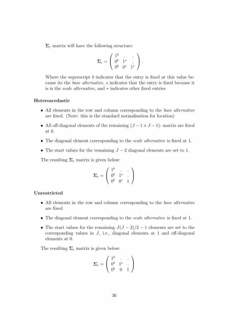
Heteroscedastic

• All elements in the row and column corresponding to the base alternativeare fixed. (Note: this is the standard normalisation for location)

• All off-diagonal elements of the remaining (J − 1× J − 1)- matrix are fixedat 0.

• The diagonal element corresponding to the scale alternative is fixed at 1.

• The start values for the remaining J − 2 diagonal elements are set to 1.

The resulting Σε matrix is given below:

Σε =

1b . .0b 1s .0b 0∗ 1

Unrestricted

• All elements in the row and column corresponding to the base alternativeare fixed.

• The diagonal element corresponding to the scale alternative is fixed at 1.

• The start values for the remaining J(J − 2)/2 − 1 elements are set to thecorresponding values in J , i.e., diagonal elements at 1 and off-diagonalelements at 0.

The resulting Σε matrix is given below:

Σε =

1b . .0b 1s .0b 0 1

36

Is this formulation of Σε identified? The most general structure of Σε inthe 3 alternative case in DCM is the following:

E(εε′) = Σε =

1b . .0b 1s .0b σ23 σ33

(1)

Comments: The order condition holds since we have J(J − 1)/2 − 1 = 2 freecovariance parameters in Σε. However, if we consider the discrete informationobserved by the analyst as imperfect measures on an underlying latent (utility)model, with the many-to-one observational rule

y = κ(y∗), (2)

where y is the index of the maximum element of the vectorJ × 1 vector y∗, thenthe realisation that the analyst will only observe the sign of y∗j − y∗j′ ∀ j 6= j′

∈ ΩJ , will have implications for the identification of the location and scale of themodel. Namely, both location and scale are defined with respect to differencesy∗j − y∗j′ .

To see this consider the following transformation. Begin with a J×J identitymatrix, and construct a matrix, ψj′ , deleting row j′, and replacing column j′ witha vector of −1′s. Using ψj′ we now construct ΣεJ−1 from the original covariancematrix, using the transformation ΣεJ−1 = ψj′Σεψ

′j′ . Taking the difference with

respect to alternative 2, we get

E(εε′) = ψ2Σεψ′2 =

(1s + 1b .σ32 + 1b σ33 + 1b

)(3)

where ε =((ε1 − ε2)(ε3 − ε2))′.

By subtracting the fixed value of variance of the base alternative (1b) from eachof the entries in (3), we see that we can retrieve the entries in the original levelserror covariance matrix in (1). Hence, the covariance specification is identified.The sum of the variances of the base and scale alternative will set the overallscale of the model.

A.3 Estimated standard errors

• Standard errors can be calculated using the inverse of the negative Hessian,

• inverse of the outer gradient product

• or using robust estimation.

37

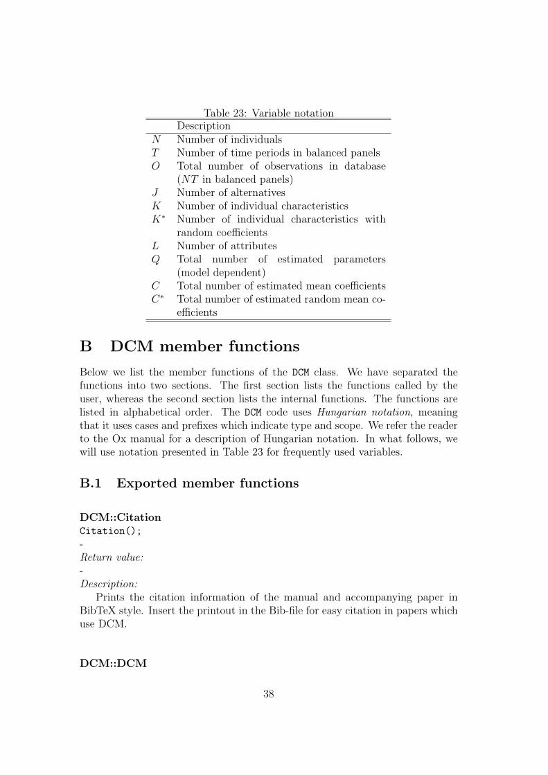
Table 23: Variable notationDescription

N Number of individualsT Number of time periods in balanced panelsO Total number of observations in database

(NT in balanced panels)J Number of alternativesK Number of individual characteristicsK∗ Number of individual characteristics with

random coefficientsL Number of attributesQ Total number of estimated parameters

(model dependent)C Total number of estimated mean coefficientsC∗ Total number of estimated random mean co-

efficients

B DCM member functions

Below we list the member functions of the DCM class. We have separated thefunctions into two sections. The first section lists the functions called by theuser, whereas the second section lists the internal functions. The functions arelisted in alphabetical order. The DCM code uses Hungarian notation, meaningthat it uses cases and prefixes which indicate type and scope. We refer the readerto the Ox manual for a description of Hungarian notation. In what follows, wewill use notation presented in Table 23 for frequently used variables.

B.1 Exported member functions

DCM::CitationCitation();

-Return value:-Description:

Prints the citation information of the manual and accompanying paper inBibTeX style. Insert the printout in the Bib-file for easy citation in papers whichuse DCM.

DCM::DCM

38

DCM();

-Return value:

-Description:

Constructor function.

DCM::DeSelectByNameDeSelectByName (const sVar, const iGroup, const iLag);sVar in: string, name of variable to de-select.iGroup in: int, group where sVar is included.iLag in: int, lag-length to de-select.

Return value:-

Description:De-selecting variables from group iGroup. This overrides Modelbase::DeSelectByName()

in order to handle the situation where variable names are not unique.

DCM::DeterministicDeterministic (bDet);bDet in: boolean, TRUE/FALSE (default).

Return value:-

Description:Creates alternative specific dummies. The default names of the dummies are

ALT 0, ALT 1, . . . . See also SetAltNames().

DCM::GenerateGenerate();

-Return value:

-Description:

Generates the dependent variable if the simulation model is properly speci-fied. The dependent variable is named ”y” and automatically appended to thedatabase. The dependent variable is automatically selected into the model.

39

DCM::Get...Get...-

-Return value:

Function call: Return value:GetAlgorithm() string with optimization routine, e.g.

”BHHH ”.GetAllResults() 5×1 array with parameter names, estimates,

standard errors, log likelihood value, andnumber of observations.

GetAltNames() J × 1 array of strings (names of alternatives)GetRefAlt() index of base alternative (m iBaseAlt ).GetCoeffType() C×1 array of strings. The type of coefficient

distribution.GetCorr() 2×1 array. The first element returns the cor-

relation matrix of random coefficients, andthe second element returns the correlationmatrix of errors.

GetCov() 2× 1 array. The first element returns the co-variance matrix of random coefficients, andthe second element returns the covariancematrix of errors.

GetcT() number of observations NT .GetErrDist() J×J matrix with non-zero values in positions

of free error covariance elements.GetNest() #nests × 1 array of vectors with nesting

structure.GetParDist() C × C matrix with 0 in diagonal positions

of non-estimated coefficients, 1 in diagonalpositions of normal distributed coefficients, 2in diagonal position of log-normal distributedcoefficients. Non-zero off-diagonal elementsindicates estimated covariances.

GetRandom() string, type of random draws.GetScaleAlt() returns index of scale alternative

(m iScaleAlt ).

Description:Some Get... functions can only be called after a successful estimation.

DCM::GetEveryVarGetEveryVar(asName );

40

asName in: k×1 array of strings. Names of variablesin data base.

Return value:Returns a n× k∗ matrix where n is the number of rows and k∗ is the number

of columns in the database representing the variables indicated by asName .Description:

GetEveryVar() checks the entire database for multiple occurrences of the el-ements in asName . As the GetVar(asNames ) command only returns the firstoccurrence of the elements in asNames , it cannot be used in the case where sev-eral columns in the data base have identical names. GetEveryVar(asNames )

ensures that all columns are returned.

DCM::InteractInteract(const asI, const asA);asI in: k × 1 array of strings.asA in: l × 1 array of strings.

Return value:-

Description:Appends and includes the kl interaction terms constructed from the variables

listed in asI and asA in the model. RemoveInteract() removes all interactionterms. Re-initialization of data may be required. Multiple calls to Interact()

accumulates interaction terms.

DCM::LoadLoad(const sDatafile);

-Return value:

-Description:

Loads the data file sDatafile and calls SetDbName(sDatafile).

DCM::OutputLaTeXOutputLaTeX(...);

41

aM0 optional in: 5× 1 array. aM0[0] q × 1 arrayof parameter names, aM0[1] q × 1 vector ofestimates, aM0[2] q × 1 vector of estimatedstandard errors, aM0[3] scalar with final loglikelihood, aM0[4] scalar with no. of obser-vations.

aM1 optional, as aM0 , and refer to another modelestimation.

If no input arguments, DCM will use the most recent estimation results to createa table.Return value:

-Description:

Produces a LaTeX table which can be inserted directly into a LaTeX docu-ment. Use of this command with multiple arguments creates one multicolumntable combining all results. Asterix indicates significance levels 10 and 1 per cent.Table .

DCM::RemoveInteractRemoveInteract();

-Return value:

-Description:

Removes all interaction terms.

DCM::ScaleVarScaleVar (const aScaleVar);aScaleVar in: 2p × 1 array sVar,dScale where sVar

is a string and dScale is a p × 1 vector ofscaling factors.

Return value:-

Description:Scale the variables listed in aScaleVar according to the associated dScale

factors. To re-set all scalings use ScaleVar();.Example: ScaleVar("Var1",0.01,"Var2",0.1) will result in the transforma-tion 0.01∗V ar1 and 0.1∗V ar2 (if previously selected or created using Interact()).

42

DCM::SetAlgorithmSetAlgorithm (iAlgorithm);iAlgorithm in: int. Specifies the optimization algorithm

to be used in estimation. See options below.

Return value:-

Description:BHHH BHHH optimizer that comes with DCM (de-

fault).BFGS Ox’s intrisinc MaxBFGS optimizer.NEWTON Ox’s intrisinc MaxNewton optimizer.

DCM::SetAltNamesSetAltNames (const asAltNames);asAltNames in: an array of strings, providing names for

alternatives in the choice set.

Return value:-

Description:Sets the names of the alternatives.

DCM::SetCoeffDistSetCoeffDist (const iType,const asPar,const iGroup);iType in: int, type of distribution. See options be-

low.asPar in: an array of strings, providing names of

mean coefficients.iGroup in: int (optional), coefficients included in the

same group (except group 0) are allowed tocorrelate.

Return value:-

Description:Sets the mixing distribution of specific coefficients in the model, together with

the correlation structure of the random coefficients. Multiple calls to SetCoeffDist()accumulates distributions.

43

FIXED Fixed (non-random) coefficients (default).NORMAL Normal distributed coefficients.(-)LOGNORMAL Log-normal distributed coefficients. Note

that the log-normal distribution has a pos-itive support. Hence, to model e.g. a nega-tive price-effect, create a price variable witha negative support or prefix with a ”-” sign.

Example: SetCoeffDist(NORMAL,"Par1","Par2",1);Example: SetCoeffDist(-LOGNORMAL,"Par3",1);sets the distributions of parameters ”Par1” and ”Par2” to multivariate normalwith non-zero correlation, and the distribution of ”Par3” to univariate log-normalwith negative support of distribution. All three coefficients are allowed to corre-late as they are included in the same group (=1).

DCM::SetDimSetDim(cN,cT,cJ);cN in: scalar, no. of individualscT in: scalar, no. of time periodscJ in: scalar, no. of alternatives

Return value:-

Description:Sets the dimension of the database when simulating discrete choice data. The

command creates the database and appends a temporary variable that indicatesthe structure of the database.

DCM::SetErrDistSetErrDist(const iType);iType in: int, type of error covariance matrix in

MNP models. See options below.

Return value:-

Description:Sets the structure of the error covariance matrix. See Appendix A.2 for a

comprehensive discussion on the error covariance structure in MNP models.

44

IID iid errors. No free error variance-covarianceelements (default).

HETEROSC Heteroscedastic errors. J − 2 free error vari-ance; no free covariance elements.

UNREST Unrestricted errors. J(J−1)/2−1 free errorvariance-covariance elements.

DCM::SetIDSetDim(sVar );sVar in: string, variable name of individual iden-

tifierReturn value:

-Description:

For unbalanced panels (and balanced panels in OxPack) DCM needs one vari-able that identifies the individual. This variable is set by SetID(). DCM willuse this variable to make inference on database structure.

DCM::SetModelSetModel(const iModel);iModel in: int, type of model. See options below.

Return value:-

Description:Sets the type of model. The options are:

CL Conditional/multinomial logit (default) (J − 1)K + L = CNL Nested logit C + #nestsMXL Mixed logit C + C(C + 1)/2MXP Mixed probit C + C(C + 1)/2MNP Multinomial Probit C + C(C + 1)/2 + J(J − 1)/2− 1OP Ordered probit C + J − 1OMP Ordered mixed probit C + C(C + 1)/2 + J − 1

DCM::SetNestSetNest(const avNest);avNest in: array of vectors, nesting structure.

Return value:-

45

Description:Sets the nesting structure.

Example: SetNest(<0>,<1,2,3>) puts alternative 0 in one nest and alternatives1, 2, and 3 in a second nest. A large number of nests can be created, but thebeta version only supports a single level of nesting, i.e., the beta-version does notsupport nests within nests.

DCM::SetPanelSetPanel (const cT);cT in: int, number of time periods in balanced

panel data. Default value=1.

Return value:-

Description:Note that the panel features in DCM 1.0 are quite primitive. The basic effect

of setting the panel is that random draws are repeated across time periods foreach individual.

DCM::SetRandomSetRandom(const iType, const cR);iType in: int, type of random numbers.cR in: int, number of random draws used in sim-

ulations. Default value=50.

Return value:-

Description:Sets the types and number of random draws.

UNIFORM Standard uniform pseudo-random numbers.HALTON Halton sequence based on primes (default).NONE Use Ox intrinsic integration routines based

upon multivariate normal probabilities.

DCM::SetRefAltSetRefAlt (const iRefAlt);iRefAlt in: int, index of base alternative 0, . . . , J−1.

Default value=0.or: string, name of reference alternative.

Return value:

46

-Description:

The iRefAlt is used as the reference alternative. The alternative specific co-efficient (associated with an individual characteristic) for the iRefAlt alternativeis set to zero. The off-diagonal elements in the iRefAlt’th row and column inthe error covariance matrix will be set to zero, and the diagonal element will beset to unity. See Appendix A.2 for details concerning the error covariance matrixin MNP models.

DCM::SetScaleAltSetScaleAlt(const iScaleAlt);iScaleAlt in: int, index of scaling alternative. Default:

second alternative (iScaleAlt=1).or: string, name of scale alternative

Return value:-

Description:Sets the alternative used for setting the scale of MNP models. This can-

not be the same as iRefAlt (see SetRefAlt()). The diagonal element in thecholesky decomposition of the error covariance matrix corresponding to alterna-tive iScaleAlt is set to 1.

DCM::SetStartParSetStartPar(const vP);vP in: Q× 1 vector, starting values for iterative

optimization algorithms.

Return value:-

Description:Let there be J alternatives, K characteristics, L attributes, and M nests. The

vector of start values is then organized as coefficients associated with J−1 alterna-tive specific constants, K(J−1) characteristics, L attributes, J−1 thresholds, Minclusive values, K(K+1)/2 elements in stacked columns of the lower cholesky de-composition of the coefficient covariance matrix, and J(J +1)/2 stacked columnsof the lower cholesky decomposition of the error covariance matrix. The vector ofparameters can either conform with the number of free (estimated) parametersor the total number of model parameters.

DCM::SetStdErr

47

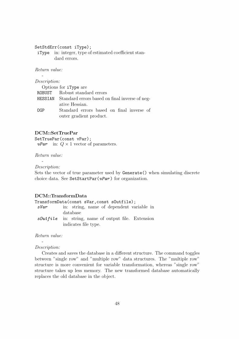
SetStdErr(const iType);iType in: integer, type of estimated coefficient stan-

dard errors.

Return value:-

Description:Options for iType are

ROBUST Robust standard errorsHESSIAN Standard errors based on final inverse of neg-

ative Hessian.OGP Standard errors based on final inverse of

outer gradient product.

DCM::SetTrueParSetTruePar(const vPar);vPar in: Q× 1 vector of parameters.

Return value:-

Description:Sets the vector of true parameter used by Generate() when simulating discretechoice data. See SetStartPar(vPar ) for organization.

DCM::TransformDataTransformData(const sVar,const sOutfile);sVar in: string, name of dependent variable in

databasesOutfile in: string, name of output file. Extension

indicates file type.

Return value:-

Description:Creates and saves the database in a different structure. The command toggles

between ”single row” and ”multiple row” data structures. The ”multiple row”structure is more convenient for variable transformation, whereas ”single row”structure takes up less memory. The new transformed database automaticallyreplaces the old database in the object.

48

DCM::TestRandCoeffTestRandCoeff(const asPar );asPar in: array of strings or int, names of coeffi-

cients.

Return value:-

Description:Tests the coefficients listed in asPar for unobserved heterogeneity. If asPar =-1

all coefficients are tested.

B.2 Non-exported member functions

DCM::CovarCovar ();

-Return value:

Returns TRUE if successful, FALSE otherwiseDescription:

Estimates the covariance matrix of parameter estimates and sets the value ofthe Q×Q covariance matrix m mCovar. The covariance matrix is calculated fromthe inverse of the negative Hessian at the point of convergence. If this matrixdoes not converge, m mCovar is constructed from the inverse of the outer gradientproduct.

DCM::fCLogitfCLogit (const vP, const adfunc, const avScore, const amHess);vP in: Q× 1 vector of parameter values.adFunc in: address of variable.

out: NT × 1 vector of individual contribu-tions to sample log-likelihood evaluated atvP.

avScore in: address of variable, or 0.out: NT × Q matrix of individual contri-butions to sample score evaluated at vP ifavScore 6=0, 0 otherwise.

amHess in: address of variable, or 0.out: Sample Hessian evaluated at vP ifamHessian 6= 0, 0 otherwise.

49

Return value:Returns TRUE if successful, FALSE otherwise.

Description:Calculates individual contributions to sample log-likelihood values and sample

scores. The same structure of arguments applies to fNestedLogit(), fMixedLogit(),fProbit(), fOProbit (), fOMProbit(). The member functions with the postfix”SQP” are wrapper functions adapted to Ox maximization functions where thesample log-likelihood (double valued) and score (vector valued) is required.

DCM::fGHKfGHK(const mD, const mW, const mU, const avV);mD in: J − 1× 2 matrix with integration limits.mW in: J − 1× J − 1 covariance matrix.mU in: J − 1 × R matrix with pseudo random

draws.avV in: address of variable.

out: J−1×R matrix of simulated truncatedmultivariate normal draws.

Return value:Returns a 1×R vector with simulated normal truncation probabilities.

Description:Implements the Geweke-Hajivassiliou-Keane (GHK) simulator.

DCM::fHaltonfHalton (const r, const c);r in: int, number of rows.c in: int, number of columns

Return value:Returns the r × c matrix of Halton draws based on the first r primes and

dropping the first 10 elements in the sequence.Description:

Generates a Halton sequence based on the first 13 primes.

DCM::fMapFreetoParfMapFreetoPar (const vFreePar);vFreePar in: Q× 1 vector of free (estimated) parame-

ters.Return value:

50

If m iModel=CL 1× 1 array, vBetaOP 2× 1 array, vBeta,vAlphaOMP 3× 1 array,vBeta,vAlpha,mCbetaNL 2× 1 array, vBeta,vLambdaMXL 2× 1 array,vBeta,mCbetaMNP 3× 1array, vBeta,mCbeta,mCeps

wherevBeta out: C × 1 vector of mean coefficients.vAlpha out: J − 1× 1 vector of threshold estimates.vLambda out: #nests× 1 vector of inclusive values.mCbeta out: C×C matrix. Lower triangular cholesky

decomposition of random coefficient covari-ance matrix.

mCeps out: J×J matrix. Lower triangular choleskydecomposition of error covariance matrix.

Description:Maps free (estimated) parameters to the full set of model parameters.

DCM::GetStartParGetStartPar()

-Return value:

Returns TRUE if successful, FALSE otherwise.Description:

This function creates starting values for MXL, MXP, MNP, and OMP modelsusing CL for unordered and OP for ordered models. The starting values of stan-dard deviations of random coefficients are set to 0.1 and 0 for covariance terms.The starting values for error standard deviations is set to 1 and 0 for covariances.DCM creates a temporary object to perform the estimations.

DCM::InitDataInitData();

-Return value:

Returns TRUE if successful, FALSE otherwise.Description:

Initializes the matrices of dependent and independent variables using the in-formation submitted in the Determinstic(), Select(), and Interact() com-

51

mands. The internal organization of the data matrices are NTJ ×K + L + 1 forunordered models and NT ×K + L + 1 for ordered models.

DCM::InitParInitPar ();

-Return value:

Return TRUE if successful, FALSE otherwise.Description:

Initializes the relevant parameters for the specified model.

DCM::IsUnivariateIsUnivariate();

-Return value:

Returns FALSEDescription:

Some data organizations in discrete choice models require multiple columnsfor the dependent variable. If DCM encounters this form of data this functionreturns FALSE.

DCM::SetParDistSetParDist (const mFreeParCov,...);mFreeParCov in: int, or C×1 vector, or C×C matrix, with

integers defining the coefficient distributions.

Return value:-

Description:Internal function handling the bookkeeping of random coefficients. Sets the

member variable m mFreeParCov.

52

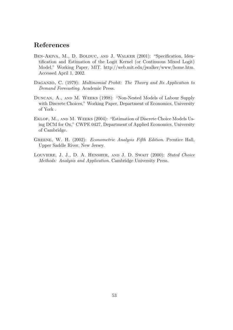
References

Ben-Akiva, M., D. Bolduc, and J. Walker (2001): “Specification, Iden-tification and Estimation of the Logit Kernel (or Continuous Mixed Logit)Model,” Working Paper, MIT. http://web.mit.edu/jwalker/www/home.htm.Accessed April 1, 2002.

Daganzo, C. (1979): Multinomial Probit: The Theory and Its Application toDemand Forecasting. Academic Press.

Duncan, A., and M. Weeks (1998): “Non-Nested Models of Labour Supplywith Discrete Choices,” Working Paper, Department of Economics, Universityof York .

Eklof, M., and M. Weeks (2004): “Estimation of Discrete Choice Models Us-ing DCM for Ox,” CWPE 0427, Department of Applied Economics, Universityof Cambridge.

Greene, W. H. (2002): Econometric Analysis Fifth Edition. Prentice Hall,Upper Saddle River, New Jersey.

Louviere, J. J., D. A. Hensher, and J. D. Swait (2000): Stated ChoiceMethods: Analysis and Application. Cambridge University Press.

53

Documents

Discrete Choice Models (DCM): An Object-Oriented Package ... · Discrete Choice Models (DCM): An Object-Oriented Package for Ox Matias Ekl˜of Department of Economics Uppsala University,