1

Discrete and integer valued inputs and outputs

in data envelopment analysis*

Timo Kuosmanen1, Abolfazl Keshvari

1, Reza Kazemi Matin

2,

1) Aalto University School of Business, Helsinki, Finland

2) Department of Mathematics, Islamic Azad University, Karaj Branch, Karaj, Iran

Abstract:

Standard axioms of free disposability, convexity and constant returns to scale employed in Data

Envelopment Analysis (DEA) implicitly assume continuous, real-valued inputs and outputs.

However, the implicit assumption of continuous data will never hold with exact precision in real

world data. To address the discrete nature of data explicitly, various formulations of Integer DEA

(IDEA) have been suggested. Unfortunately, the axiomatic foundations and the correct

mathematical formulation of IDEA technology has caused considerable confusion in the literature.

This chapter has three objectives. First, we re-examine the axiomatic foundations of IDEA,

demonstrating that some IDEA formulations proposed in the literature fail to satisfy the axioms of

free disposability of continuous inputs and outputs, and natural disposability of discrete inputs and

outputs. Second, we critically examine alternative efficiency metrics available for IDEA. We

complement the IDEA formulations for the radial input measure with the radial output measure and

the directional distance function. We then critically discuss the additive efficiency metrics,

demonstrating that the optimal slacks are not necessarily unique. Third, we consider estimation of

the IDEA technology under stochastic noise, modeling inefficiency and noise as Poisson distributed

random variables.

Key words:

Axiomatic production theory; Efficiency analysis; Mixed integer linear programming; Stochastic

noise

* Abbreviations of key concepts referred to in this chapter: DEA = Data Envelopment Analysis, DMU = Decision

Making Unit, CNLS = Convex Nonparametric Least Squares, IDEA = Integer DEA, MILP = Mixed Integer Linear

Programming, RTS = Returns To Scale, SFA = Stochastic Frontier Analysis, StoNED = Stochastic Nonparametric

Envelopment of Data.

Abbreviations of articles frequently cited in this chapter: KJM = Kuosmanen, Johnson and Saastamoinen (in this

volume), KKM = Kuosmanen and Kazemi Matin (2009), KMK = Kazemi Matin and Kuosmanen (2009), KSM =

Khezrimotlagh, Salleh, and Mohsenpour (2012, 2013a, 2013b), LV = Lozano and Villa (2006, 2007).

2

1. Introduction

Data envelopment analysis (DEA, Charnes et al., 1978) is an axiomatic, mathematical programming

approach to assessing efficiency of decision making units (DMUs).1 DEA does not assume any

particular functional form for the frontier, but relies on the axioms of production theory, most

importantly, free disposability, convexity, and some specification of returns to scale (i.e., variable,

non-increasing, non-decreasing, or constant). The standard axioms of free disposability, convexity

and constant returns to scale employed in DEA implicitly assume continuous, real-valued inputs

and outputs. In contrast, input-output data used in applications are always discrete because the

precision of measurement is necessarily restricted to a limited number of decimal digits. Therefore,

the implicit assumption of continuous data will never hold with exact precision in real world data.

From a practical point of view, this is not a problem if the observed discrete data can be

meaningfully approximated by continuous variables. For example, if the labor input is measured by

the number of hours worked, rounded to the nearest integer, and the measured input varies between

1,000 hours and 100,000 hours across evaluated DMUs, then the continuous approximation of the

discrete data of labor input is perfectly valid as the possible rounding error is small (at most 0.1%)

relative to the measured input. In contrast, if the labor input is the number of workers performing

certain function (e.g., firm managers, university professors, hospital physicians), and the DMUs

under evaluation are small, the rounding error can become a significant issue. For example,

Kuosmanen and Kazemi Matin (2009) consider efficiency analysis of university departments where

the number of professors and the number of published articles are examples of integer valued input

and output variables. Suppose a university department currently has three professors. Suppose

further that the conventional DEA analysis suggests the efficient level of professors is 2.7. How

should this result be interpreted? If we round up the efficient number of professors to 3, then the

evaluated DMU will appear as efficient, even though the DEA analysis indicates input efficiency of

90 percent. However, rounding the input target downwards to 2 may result as an infeasible solution.

Since the conventional DEA implicitly assumes all inputs and outputs to be real-valued, the

estimated DEA frontier does not necessarily provide meaningful reference points if one simply

rounds the input or output targets to the nearest whole number.

1 We will henceforth use the term “DMU” to refer to any entity that transforms inputs to output, including both non-

profit firms and for-profit companies. DMU can refer to a production plant, facility, or sub-division of a company, or to

an aggregate entity such as an industry, a region, or a country.

3

Lozano and Villa (2006, 2007) (henceforth LV) were the first to address this issue explicitly

in DEA.2 They proposed to estimate the production possibility set as the intersection of the standard

DEA technology and the set of non-negative integers. Unfortunately, they did not provide any

theoretical justification for their integer DEA (henceforth IDEA) technology, even though it is

obvious that the proposed technology does not satisfy the standard axioms of free disposability or

convexity. To address this problem Kuosmanen and Kazemi Matin (2009) (henceforth KKM)

introduced two new axioms of natural disposability and natural divisibility. Imposing the classic

additivity axiom (Koopmans 1951), KKM proved that LV’s constant returns to scale (CRS)

technology has a sound axiomatic foundation. Specifically, they showed that the IDEA technology

is the smallest set that contains all observed data points and satisfies the axioms of additivity,

natural disposability, and natural divisibility. Subsequent paper by Kazemi Matin and Kuosmanen

(2009) (henceforth KMK) extended the result to the variable returns to scale (VRS) case,

introducing the axiom of natural convexity.

Another contribution of LV is the development of a mixed integer linear programming

(MILP) DEA formulation to measure efficiency of DMUs relative to the IDEA technology using

Farrell’s (1957) radial input-oriented measure. KKM argue that the classic Farrell measure needs to

be modified in the context of integer-valued input-output data, and propose to measure efficiency as

the radial distance to the monotonic hull of the IDEA technology. They further argue that LV’s

MILP formulation over-estimates efficiency, and they demonstrate their argument by means of a

numerical example and an application.

Following the pioneering works by LV and KKM, a number of extensions and applications of

integer DEA have been published (see, e.g., Wu et al. 2009; 2010; Lozano et al. 2011; Kazemi

Matin and Emrouznejad, 2011; Alirezaee and Sani 2011; Chen et al., 2012; Du et al., 2012; Nöhren

and Heinzl, 2012; Lozano, 2013; Chen et al., 2013). We will survey the extensions and applications

in more detail Section 8 of this chapter.

Unfortunately, the axiomatic foundation and the MILP formulation of integer DEA have also

caused serious confusion since the original works by LV. Recently, a series of papers by

Khezrimotlagh, Salleh, and Mohsenpour (2012, 2013a, 2013b) (henceforth KSM) have contributed

to further confusion by discrediting the contributions of KKM and disregarding both the importance

of a sound axiomatic foundation and rigorous mathematical formulations. While the bogus critique

by KSM is not worth serious consideration, the naïve mistakes of KSM provided us some further

2 Previous studies such as Banker and Morey (1986), Kamakura (1988), and Rousseau and Semple (1993) (among

others) consider inputs and outputs measured on the categorical or ordinal scale, which are obviously integer valued.

However, input-output variables defined on the interval or ratio scales can be integer valued as well.

4

motivation to elaborate our arguments and shed some new light on the intimate connection between

the axioms of production theory and the implementation through MILP.

The purposes of this chapter are three-fold. First, we re-examine the axioms and MILP

formulations of integer DEA, elaborating some aspects that have apparently caused confusion in the

literature. Emphasizing the importance of the axiomatic foundation, we demonstrate that LV’s

MILP formulations fail to satisfy the axioms of free disposability of continuous inputs and outputs,

and natural disposability of discrete inputs and outputs. We illustrate the inconsistency of LV’s

MILP formulation with the IDEA technology they suggested through detailed numerical examples,

which demonstrate the differences between the LV’s formulation and those developed by KKM and

KMK.

Second, we critically examine alternative efficiency metrics available for integer DEA. We

complement the MILP formulations for the radial input oriented Farrell (1957) measure proposed

by KKM and KMK with the radial output oriented measure, and the general directional distance

function (Chambers et al., 1996, 1998). We then critically discuss the additive efficiency metrics

considered by LV (2007), demonstrating that the optimal slacks are not necessarily unique. The

same problem applies to the range adjusted additive measure proposed by Cooper et al. (1999). The

non-uniqueness of slacks can make the application of the slack based measure by Tone (2001)

problematic in the context of integer DEA.

Third, attributing all deviations from the frontier to inefficiency, ignoring stochastic noise, is

generally recognized as the main limitation of DEA (see Kuosmanen, Johnson and Saastamoinen, in

this volume, (henceforth KJM) for a review of recent advances in modeling noise). To address this

shortcoming, we examine the estimation of the IDEA technology in the single output setting under

stochastic noise. Modeling inefficiency and noise as Poisson distributed random variables, we

outline the first extension of stochastic nonparametric envelopment of data (StoNED) approach by

Kuosmanen and Kortelainen (2012) to discrete output variables.

The rest of this chapter is organized as follows. Section 2 introduces and discusses the axioms

for a DEA problem with integer-valued inputs and outputs. Section 3 derives the associated DEA

production sets that satisfy the fundamental minimum extrapolation principle,3 and generalize the

method to the hybrid case where both real and integer valued inputs and outputs are present. Section

4 modifies the Farrell input efficiency measure to the integer DEA setting, and show how the

efficiency score can be computed by solving a MILP problem. Section 5 discusses new

developments on integer DEA and some extensions. Section 6 presents concluding discussion with

3 The minimum extrapolation principle was formally introduced by Banker et al. (1984), but formal minimum

extrapolation theorems (and proofs) date back at least to Afriat (1972).

5

some potential avenues for future research. The paper includes several theorems: proofs of all

theorems and lemmas are presented in the Appendix.

2. Axioms

The axiomatic approach to constructing production possibility sets as a combination of observed

activities has a long history in economics, dating back at least to Von Neumann (1945-1956) and

Koopmans (1951). Afriat (1972) was the first to prove the minimum frontier production functions

that envelop all observed data and satisfy the following sets of axioms: i) free disposability, ii)

convexity and free disposability, and iii), CRS, convexity and free disposability. Banker et al.

(1984) extended Afriat’s result to the multi-output production possibility sets, and formally

introduced the fundamental minimum extrapolation principle.

Multi-output production technology can be generally characterized by the production

possibility set defined as

{( )|

},

where x is a m-dimensional vector of input quantities and y is a s-dimensional vector of output

quantities.4 Intuitively, the set T can be understood as a list of feasible input-output combinations.

Even if we restrict to discrete or integer valued input-output vectors, in general, there are infinitely

many feasible input-output vectors, which makes the list infinitely long. It is worth emphasizing

that, in many applications, the production possibility set T is interpreted as the benchmark

technology that forms a reference for performance comparisons and efficiency analysis. In this

interpretation, the boundary of set T characterizes standards for good performance, not only the

production possibilities from the strictly technical point of view.

Observed DMUs are characterized by a pair of non-negative input and output vectors ( )

{ }. Conventional DEA approaches implicitly assume that all inputs and outputs are

continuous, real-valued variables. However, observed data are always discrete as the number of

decimal digits is necessarily finite. This forms the motivation for integer DEA. Note that any

discrete data that cannot be meaningfully approximated as continuous data can easily be converted

to integers by a simple multiplicative transformation. Suppose, for example, that a continuous

output variable is measured at the precision of one decimal digit (e.g., 0, 0.1, 0.2, …), but rounding

the DEA targets to the nearest decimal digit seems problematic for one reason or another. This

4 For clarity, we denote vectors by bold lower case letters (e.g., x) and matrices by bold capital letters (e.g., X).

6

discrete output variable can be harmlessly multiplied by factor 10 (amounting to a change of units

of measurement), which results as an integer valued output variable.

In the following we will focus on integer-valued inputs and outputs ( ) , which lead

us to integer DEA (IDEA) introduced by LV. In the following sub-sections we will adapt the classic

axioms of DEA to allow for integer valued inputs and outputs, following KKM and KMK.

2.1 Free disposability and natural disposability

Free disposability is an intuitive and widely used axiom. It is closely related to monotonicity of

functional representations of technology: free disposability implies that the production function is

monotonic increasing in inputs and the cost function is monotonic increasing in outputs. It is

possible to assess efficiency relying solely on the free disposability axiom, using the free disposable

hull (FDH) method (Deprins et al., 1984; Tulkens, 1993). However, free disposability is not always

a meaningful axiom. For example, if the output vector y includes undesirable outputs (bads) such as

waste or pollution, the free disposability axiom can be replaced by the weak disposability axiom.5

Free disposability is also relaxed for modeling congestion. 6

The axiom of free disposability is conventionally stated as follows:

(A1) Free disposability: ( ) and ( ) , ( ) .

This axiom states that it is always possible to produce less output with a given level of inputs, or

alternatively, use more inputs to produce the same amount of output. Vector u can be interpreted as

the amount of excess inputs used, and vector v represents the foregone output. If we interpret this

axiom literally, it seems impossible to consume infinite amounts of inputs in a finite production

process. Hence axiom (A1) is not necessarily valid from a strictly technical point of view. However,

it does have a compelling economic interpretation: (A1) essentially states that inefficient production

(in the sense of Koopmans, 1951) is feasible. Stated differently, if our objective is to assess

technical efficiency in the sense of Koopmans (1951), and we interpret T as a benchmark

technology rather than as a list of technically feasible points, then (A1) is a completely harmless

axiom irrespective of whether it is technically feasible or not.

5 The correct way of implementing weak disposability in DEA has caused some confusion in the literature: see

Kuosmanen (2005), Färe and Grosskof (2009), Kuosmanen and Podinovski (2009), and Podinovski and Kuosmanen

(2011) for an interesting debate on this issue. 6 This is another issue that has caused confusion: see Cherchye et al. (2001).

7

Axiom (A1) implies continuity. Clearly, if this axiom holds, then there are feasible real-

valued input-output vectors ( ) that are not included in . Stated conversely, if the

production possibility set T contains only integer-valued input-output vectors, then it cannot satisfy

the standard free disposability axiom. Therefore, it is necessary to adapt this axiom to be consistent

with integer-valued inputs and outputs. KKM propose the following axiom:

(B1) Natural disposability: ( ) and ( ) , ( ) .

The economic rationale of axiom (B1) is exactly the same as that of the standard free disposability

axiom (A1): inefficient production is feasible. However, (B1) only allows for integer-valued

disposal of outputs through vector v and integer-valued excess inputs through vector u. Therefore,

axiom (B1) is a suitable counterpart of (A1) that applies for integer valued inputs and outputs.

2.2 Convexity and natural convexity

The classic DEA approaches (Farrell, 1957; Charnes et al., 1978; Banker et al., 1984) impose

convexity in addition to free disposability. The standard convexity axiom can be stated as follows:

(A2) Convexity: ( ) ( ) ( ) ( ) ( )( ) ( ) .

This axiom states that convex combinations of observed DMUs are always feasible. The weights

assigned to the observations are characterized by parameter . In general, we can form convex

combinations of all n observations in J using a n-dimensional parameter vector .

Convexity does not necessarily have a strong justification from the strictly technical point of

view, but it is a fundamental axiom in economic theory. For example, convexity is critically

important for establishing duality results between alternative representations of technology

(Shephard, 1970; Färe and Primont, 1995). For example, if the profit function of a firm is known,

we can always recover the convex hull of its production possibility set T (see Kuosmanen, 2003, for

details). If we interpret T as a benchmark technology for competitive profit maximizing firms that

take prices as given, then convexity is an equally harmless axiom as free disposability. However, if

we consider nonprofit firms or monopolistic competition, convexity may be a restrictive assumption

as it assumes away economies of scale (see, e.g., Kuosmanen, 2001). Weaker forms of quasi-

convexity (i.e., convex input or output sets) have also been considered in the DEA literature (e.g.,

Petersen, 1990; Bogetoft, 1996; Bogeoft et al., 2000; Post, 2001).

8

Clearly, if axiom (A2) holds, then there are feasible real-valued input-output vectors ( )

that are not integer-valued. Conversely, if the production possibility set T contains only integer-

valued input-output vectors, then it violates convexity. Therefore, it is necessary to adapt this axiom

to be consistent with integer-valued inputs and outputs. KMK propose the following axiom:

(B2) Natural convexity: ( ) ( ) ( ) ( ) ( )( )

( ) ( ) .

Analogous to the pair of axioms (A1) and (B1), the rationale of axiom (B2) is to adapt (A2) to the

context of integer-valued inputs without changing its meaning. Note that (B2) only adds to (A2) the

requirement that ( ) , that is, the resulting convex combination must itself be integer-

valued. Note that KMK allow the weights used for forming convex combinations to be real

valued. They do not see a problem in using real valued numbers in the mathematical operations

involved in the axioms as far as the resulting input-output vectors are integer-valued.

KSM (2012) criticize KMK for the use of real valued weights for forming convex

combinations.7 They propose to substitute weights in (B2) by the ratio , such that ,

. Mathematically, this restricts the domain of weights from the real numbers to the

set of rational numbers. Therefore, the alternative axiom proposed by KSM does not expand the

production possibility set, it can only contract it. In fact, we can prove the following:

Lemma 1: Assume Axiom (B2) is satisfied. Then for any given ( ) ( ) , if there exists a

real valued such that ( ) ( ) ( )( ) , then there exist integers

, , such that

.

This lemma shows that the alternative convexity axiom proposed by KSM makes no

difference whatsoever. If one finds the axiom by KSM more aesthetic or elegant, one can

harmlessly use it, without a need to revise the theory developed by KKM. However, for the sake of

intuition and transparency, we prefer to maintain a close connection between the axioms for real

valued and integer valued variables (i.e., axioms A and axioms B). Since there is no real benefit

7 KSM (2012) state: ”Now, if it has been supposed that only the integer numbers set is considered, then it should not

have been used the real number variable in the integer axioms! In fact, a new axiom must not have any doubts or

parallel affects with those previous axioms. In other words, an axiom is an evident premise as to be accepted as true

without controversy.” This discussion reveals that KSM do not understand the economic meaning of axioms in DEA. In

fact, none of the standard DEA axioms can meet the requirements of KSM.

9

from restricting the domain of weights from the set of real numbers to the set of rational numbers,

this is only a matter of subjective preference. In this light, the claims about “major shortcomings”

that KSM repeatedly express in their papers are completely irrational.

2.3 Returns to scale

Returns to scale concerns radial contraction or expansion of all inputs and outputs by the same

factor. Note that if no axioms concerning returns to scale are imposed, then the technology is said to

exhibit variable returns to scale (VRS). To implement VRS in DEA, the weights employed for

forming convex combinations of observed DMUs must sum to one (i.e., ∑ ). When

further axioms concerning returns to scale are imposed, this constraint can be relaxed.

Consider first the radial contraction possibilities. The conventional axiom of non-increasing

returns to scale (NIRS) can be stated as follows:

(A3) Non-increasing returns to scale: ( ) and ( ) .

This axiom allows one to scale down any observed input-output vector by factor . Note that axiom

(A3) implies that inactivity is feasible: the origin (0,0) is included in the production possibility set T

because, starting from any observed ( ), we can set factor = 0. If we simply insert the origin

(0,0) as one of the observed points in the data set, then the variable returns to scale DEA technology

will automatically satisfy axiom (A3). This provides an implicit way of implementing NIRS, which

may be useful in some context (see Kuosmanen, 2005). A more standard way of implementing

NIRS in DEA is to set a constraint that the sum of intensity weights must be less than or equal to

one (i.e., ∑ ).

Clearly, even if we start from an inter-valued input-output vector ( ) , the rescaled

vector ( ) is not necessarily integer valued. Therefore, axiom (A3) is not directly applicable

for integer DEA. KKM propose to modify axiom (A3) as

(B3) Natural divisibility: ( ) and and ( ) ( ) .

Natural divisibility simply introduces an additional restriction that the downward rescaled version

of the original input-output vector must result as an integer valued production plan to be feasible.

10

Consider next the radial expansion. The conventional axiom of non-decreasing returns to

scale (NDRS) can be stated as follows:

(A4) Non-decreasing returns to scale: ( ) and ( ) .

This axiom allows for radial expansion of any observed input-output vector away from the origin by

factor . The NRDS axiom is implemented in DEA by enforcing the sum of intensity weights

to be greater than or equal to one (i.e., ∑ ).

Obviously, the rescaled vector ( ) does not have to be integer valued. Therefore, KMK

propose to adapt this axiom for integer DEA as

(B4) Natural augmentability: ( ) and and ( ) ( ) .

Natural augmentability requires that the radial expansion must result as an integer valued input-

output vector in order to be feasible.

Note that in both (B3) and (B4), KMK assume a real-valued multiplier . In both cases, we

could equally well express as a ratio of two integers.

Lemma 2: For any given ( ) , if there exists a real valued such that ( ) , then

there exist integers , , such that

.

This result again shows that the alternative formulations of the KMK axioms suggested by KSM do

not make any practical difference whatsoever.

Finally, if both (A3) and (A4) hold, then the technology is said to satisfy constant returns to

scale (CRS):

(A5) Constant returns to scale: ( ) and ( ) .

In the CRS case, the sum of intensity weights is unrestricted. Observe that imposing additional

axioms on returns to scale implies less restrictive constraints for the intensity weights , which

leads to the expansion of the estimated production possibility set.

From a strictly technical point of view, the CRS axiom appears totally unrealistic. However, it

does have compelling economic justification in many applications. If the objective of the firm is to

11

maximize profitability (i.e., the ratio of revenue to cost) at given prices, then the CRS axiom is

completely harmless (see Kuosmanen et al., 2004; Lemma 1).

KMK did not introduce an integer equivalent of (A5): note that if both (A3) and (A4) hold,

then (A5) holds. The converse is also true. Therefore, the CRS case is obtained in integer DEA by

imposing (B3) and (B4). For the sake of completeness, we can state the integer version of (A5) as

(B5) Natural radial rescaling: ( ) and and ( ) ( ) .

In fact, KKM examine the CRS case in detail, imposing the axiom of additivity (adopted from

Koopmans, 1951) in addition to natural divisibility (B3).

(A6) Additivity: ( ) ( ) ( ) .

Since axiom (A6) was first introduced in the context of continuous variables, we label it as type-A

axiom. Note, however, that the additivity axiom does not require or imply continuity, and hence it

applies equally well to integer valued inputs and outputs. Interestingly, we can build the IDEA

technology under CRS to the axioms of additivity and natural divisibility axioms, as shown by the

following result:

Lemma 3: If the axioms (B2) Natural convexity and (B5) Natural radial rescaling are satisfied,

then the axioms of (B3) Natural divisibility and (A6) Additivity must also hold. Conversely, if

axioms (B3) and (A6) are satisfied, then axioms (B2) and (B5) must also hold. In other words,

these two pairs of axioms are equivalent in the following sense:

[(B2) and (B5)] ⇔ [(B3) and (A6)] .

2.4 Envelopment

In addition to the standard axioms of production theory (e.g., Shephard, 1970; Färe and Primont,

1995), the classic DEA article by Banker et al. (1984) imposes the following axiom:

(E1) Envelopment: all observed data points ( ) are feasible: ( ) .

For clarity, we label this assumption as type-E postulate, as (E1) not really an axiom in the same

sense as (A1) – (A6) and (B1) – (B5) considered above. Note that all axioms introduced before are

conditional statements expressed using (i.e., if condition “A” holds, then “B” is feasible). In

12

contrast, (E1) is an unconditional statement about the observed data. In our interpretation, the

minimum extrapolation principle together with (E1) form the estimation principle of DEA

analogous to the minimization of least squares or the maximization of the log-likelihood function in

regression analysis.

From the strictly technical sense, (E1) is a natural and intuitive axiom: if point ( ) is

observed, then it clearly must be feasible. One could argue that this axiom is proved by empirical

evidence.

However, the fact that ( ) is observed once does not necessarily guarantee that DMU j

can replicate ( ) again in the future, or that other DMUs can achieve the point ( ). In many

applications of efficiency analysis, production process is subject to uncontrollable random elements,

including technological risks (e.g., machine failure). There are also economic risks (e.g., variation

in demand and input-output prices), and risks related to the operating environment (e.g.,

competition, regulation, weather conditions). In practice, DEA can handle a limited number of input

and output variables,8 and hence one often needs to either omit some relevant inputs or outputs, or

resort to aggregated inputs and outputs (e.g., monetary cost or revenue aggregates) that are subject

to errors of aggregation. While DEA implicitly assumes homogenous DMUs that operate in a

homogenous environment, in reality, evaluated DMUs tend to be heterogenous and operate in

heterogenous environments. The random variations, omitted variables, data errors, and

hetereogeneity are some of the possible reasons for why the envelopment condition (E1) is not valid

in applications.

The recent works by Kuosmanen (2008), Kuosmanen and Johnson (2010), and Kuosmanen

and Kortelainen (2012) demonstrate that it is possible to relax the envelopment condition (E1), and

estimate production technologies subject to some of the axioms (A1) – (A6) in a nonparametric or

semi-nonparametric fashion (see KJM for a review). We consider the CNLS (convex nonparametric

least squares) and StoNED (stochastic nonparametric envelopment of data) developed in these

papers a promising way forward. An extension of StoNED method to IDEA technology will be

developed in Section 6. To pave a way for the stochastic extension, we will maintain the assumption

(E1) in Sections 3 – 5.

To summarize this section, Table 1 lists the axioms considered, indicating the standard

axioms (A1) – (A5) that imply continuity and the corresponding axioms (B1) – (B5) for discrete,

integer-valued variables, and the other axioms / conditions.

8 DEA is a nonparametric estimator subject to the curse of dimensionality. This implies that the precision of DEA

estimator deteriorates rapidly as the number of input and output variables increases. Also the discriminating power of

DEA is affected: when the dimensionality is large, almost all DMUs appear as inefficient.

13

Table 1: Axioms considered in this paper

Axioms that imply continuity Corresponding axioms for discrete variables

(A1) Free disposability (B1) Natural disposability

(A2) Convexity (B2) Natural convexity

(A3) Non-increasing returns to scale (B3) Natural divisibility

(A4) Non-decreasing returns to scale (B4) Natural augmentability

(A5) Constant returns to scale (B5) Natural radial rescaling

Other axioms / conditions

(A6) Additivity

(E1) Envelopment

3. Continuous, integer-valued and hybrid DEA technologies

Having introduced the axioms, we will next examine the continuous and integer-valued DEA

estimators of the production possibility set T, and a hybrid case where some inputs and outputs are

integer-valued while others are continuous.

Applying the fundamental minimum extrapolation principle, any DEA technology can be

constructed as the intersection of such sets that contain all observed DMUs (E1) and

satisfy the stated axioms (Banker et al. 1984). In the case of continuous input-output variables, the

DEA estimator of the production possibility set T can be stated as

{( )

subject to

∑ ;

∑ ;

},

where denotes the generic domain of intensity weights under alternative RTS specifications.

Specifically, can be specified by choosing one of the four options below:

{∑ }

{∑ }

{∑ }

14

{ }

This generic domain allows for alternative specifications of RTS known in the DEA literature. The

connection to the axioms introduced in Section 2 is the following. Under axioms (A1) + (A2), we

have the VRS specification . Axioms (A1) + (A2) + (A3) imply the NIRS specification ,

while axioms (A1) + (A2) + (A4) imply the NDRS specification . Under axioms (A1) + (A2)

+ (A5), we have the CRS specification .

Banker et al. (1984) formally show that set satisfies the envelopment condition (E1) and

the stated axioms, and that is the intersection of all such sets that satisfy those axioms. In this

sense, is the smallest set that satisfies the stated axioms.

9 Note that the axiom of convexity is

implemented through the use of intensity weights (compare with axiom (A2)), which allow for

any convex combination of observed DMUs. Restricting weights to be integers relaxes the

convexity axiom (A2), leading to the free disposable hull (Deprins et al., 1984) and free replicable

hull (Tulkens, 1993) technologies. The axiom of free disposability is implemented through the

inequality constraints for inputs and outputs. Replacing the inequality constraints by strict equality

would relax the free disposability axiom (A1), leading to the DEA formulations of weak

disposability (e.g. Kuosmanen 2005) and congestion (e.g. Cherchye et al. 2001).

In the case of integer-valued inputs and outputs, the generic IDEA technology first proposed

by LV can be similarly stated as

{( )

subject to

∑ ;

∑ ;

},

where is the generic domain of intensity weights under alternative RTS specifications

introduced above. In the case of the IDEA technology, axioms (B1) + (B2) imply the VRS

specification . Under axioms (B1) + (B2) + (B3) we have the NIRS specification , and

axioms (B1) + (B2) + (B4) imply the NDRS specification . Finally, the CRS specification

is obtained under axioms (B1) + (B2) + (B5).

9 In the single output case, Afriat (1972) proves the similar minimum extrapolation result for the smallest production

function satisfies axioms (A1), (A1) + (A2), or (A1) + (A2) + (A5).

15

Comparing the sets and

, it is obvious that

. LV correctly note that

.

In words, IDEA technology is the intersection of the set of integer vectors and the conventional

DEA technology, and the latter set is further an intersection of all such sets that satisfy (E1), (A1),

(A2), and the specified RTS axioms. However, it is easy to see that itself does not satisfy any

of the axioms (A1) – (A4). This is the reason why KKM criticized LV for the lack of axiomatic

foundation. It is not enough that a benchmark technology is an intersection of some arbitrary sets:

the minimum extrapolation principle requires that itself satisfies the stated axioms, and is the

smallest set that does so.

Fortunately, the axiomatic foundation can be established using the parallel set of axioms (B1)

– (B4), as shown by KKM and KMK. The minimum extrapolation theorems by KKM and KMK

can be formally summarized as follows:

Theorem 1. Production possibility set is the intersection of all sets

that satisfy the

envelopment (E1), axioms (B1) and (B2), the RTS axioms ((B3), (B4), (B5), or none) corresponding

to the specified returns to scale.

Note that axioms (B1) and (B2) could be relaxed in the same way as in the standard DEA

technology. If the inequality constraints for inputs and outputs are replaced by equality constraints,

this amounts to relaxing axiom (B1). Similarly, if intensity weights are restricted to be binary

integers, the convexity axiom (A2) is relaxed. We emphasize the direct correspondence between the

axioms and the mathematical formulations of alternative DEA technologies.

In addition to the settings where all inputs and outputs are either continuous or integer valued,

in many applications of IDEA some of the input-output variables are integer valued while others

can be meaningfully approximated as continuous variables. Following LV, KKM, and KMK, this

case will be henceforth referred to as the hybrid integer DEA (HIDEA). In general, we can partition

the set of input variables as and the set of output variables as , where

subsets and contain the integer valued inputs and outputs, respectively, whereas subsets

and include the real valued inputs and outputs. Without loss of generality, subsets and , as

well as and , are assumed to be mutually disjoint, and | | and | | .

Applying these notations, we can state any non-negative input and output vectors ( ) as

16

(

) , (

).

In the hybrid setting, we can impose type-A axioms for the continuous inputs and outputs

included in and , while type-B axioms are used for integer-valued inputs and outputs

included in and . In practice, we can formulate the HIDEA technology as

{(

)

subject to

( )

;

(

) ∑ (

)

;

(

) ∑ (

)

;

},

where are specified for VRS, NIRS, NRDS, or CRS as noted above. Note that the same set of

intensity weights are used for both integer-valued and continuous input-output variables.

However, the constraint ( )

only applies to the subset of integer-valued input-output

variables.

The next theorem generalizes the axiomatic foundation established in Theorem 1 to this

hybrid setting.

Theorem 2. Production possibility set is the intersection of all sets S that satisfy the

envelopment (E1), axioms (A1) and (A2) for the subsets ( ), axioms (B1) and (B2) for the

subsets ( ), and the RTS axioms ((A3), (A4), (A5), or none for the subsets ( ), and (B3),

(B4), (B5), or none for for the subsets ( )) corresponding to the specified returns to scale.

In addition to these symmetric cases where the real-valued and integer-valued variables

exhibit the same type of returns to scale, it could be interesting to allow the returns to scale differ

for the real-valued and integer-valued variables, in the spirit of the hybrid returns to scale

17

technology by Podinovski (2004). For example, in some applications it might be reasonable to

assume the real-valued variables are subject to VRS, while the integer-valued variables exhibit

CRS. Extending the HIDEA problem to hybrid returns to scale specifications falls beyond the scope

of the present paper, and is left as an interesting topic for future research.

4. Efficiency measures and distance functions

4.1 Modified Farrell input efficiency measure

Having introduced the IDEA and HIDEA technologies, we will next examine the measurement of

efficiency as a distance from the observed input-output vector of the evaluated DMU to the efficient

boundary of the benchmark technology. Before proceeding, we must stress that the standard

efficiency measures (including the radial Farrell input and output measures, the additive Pareto-

Koopmans efficiency measures, and the directional distance functions) all implicitly assume

continuous, real-valued inputs and outputs. Consider, for example, the classic Farrell input

efficiency measure, defined as

( ) { |( ) },

where vector ( ) is the input-output vector of the DMU under evaluation (which can be one of

the observed DMUs or a hypothetical unit of interest). Value = 1 indicates full efficiency, and

values imply the evaluated DMU is inefficient: ( ) indicates the degree of

inefficiency. Unfortunately, applying the standard Farrell measure directly to is likely

problematic because is essentially a discrete set of disconnected points. Hence, applying the

standard Farrell measure as such can yield very strange, counterintuitive results. For example, it is

possible that ( ) for input-output vector ( ) that is strictly dominated by

another point in .

To avoid complications due the discrete nature of IDEA and HIDEA technologies, KKM

propose to modify the Farrell input efficiency measure as:

( ) { | ( ) }.

This modified Farrell measure gauges radial distance to the monotonic hull of the benchmark

technology, requiring that the reference point ( ) must be dominated by a feasible input-

output vector ( ) which has integer-valued inputs for the subset . For the sake of completeness,

18

note that we could also add a requirement that

, but this would be completely redundant in

the case of input-oriented efficiency measure.

The modified input efficiency measure preserves the usual interpretation of the

Farrell measure as a downward scaling potential in inputs at the given output level. It guarantees

that DMUs assigned the efficiency score one are weakly efficient in the Pareto-Koopmans sense.

Unfortunately, the original papers by LV suggested MILP formulations for computing the radial

input- and output-oriented efficiency measures without explicit recognition of the need to modify

the efficiency metric. Therefore, it is not immediately clear what LV intend to measure in the first

place, and how the constraints of LV’s MILP formulations should be interpreted: do the inequality

constraints of LV represent the disposability axioms of the benchmark technology or the

measurement of distance to the monotonic hull of the benchmark technology? This appears to be

the source of confusion for KSM, who similarly overlook the modification of the Farrell efficiency

measured clearly stated in both KKM and KMK articles. We return to this point in more detail in

the numerical examples considered below.

4.2 MILP formulation

In the case of the general benchmark technology, the modified input efficiency measure

can be computed by solving the following MILP problem:

( )

subject to

{

∑

∑ ,

∑ ,

.

To clarify some key issues that continue to cause confusion in the IDEA literature, it is worth to

examine the interpretation and the rationale of the constraints of the MILP problem in detail,

highlighting the direct connections between the axioms introduced in Section 2 and their

implementation in the MILP formulation.

19

For clarity, the constraints of the above MILP problem have been stated as inequalities, and

the non-radial slacks have been omitted. In contrast, KKM and KMK state their MILP formulations

using equality constraints and slacks.10

This is one potential source of confusion prevailing in the

IDEA literature. In particular, KSM (2012b) have criticized the MILP formulations by KKM and

KMK for producing sub-optimal slacks. We find this critique misplaced because KKM and KMK

were mainly interested in measuring efficiency using the radial metric : the slacks were used

merely as instruments for imposing the free disposability and natural disposability axioms (A1),

(B1), and for measuring the distance to the monotonic hull of the benchmark technology. In the case

of continuous variables, we see the non-radial slacks merely as artifacts of the DEA technology,

which do not necessarily have any relation to the underlying production technology: even if the true

technology is smooth, the piece-wise linear DEA technology will have slacks. The presence of

slacks does not imply the true technology is non-smooth. In the case of IDEA technology, the non-

radial slacks may be meaningful. However, the slacks determined by the MILP problem are not

necessarily unique, and not even Pareto-Koopmans efficient, as will be demonstrated below by

means of numerical examples. For these reasons, we do not consider the non-radial slacks to be

particularly interesting or useful.

To further clarify the MILP formulation, we use curly bracket { to identify the constraints

associated with integer-valued inputs (subset II). The first constraint introduces a vector of integer-

valued variables

. Variables represent the integer-valued benchmark introduced in the

definition of : note that the elements of are optimized subject to the first and the second

constraint of the MILP problem. The first constraint states that the convex combination of the

observed DMUs must dominate the benchmark . Note that the inequality sign stated in the first

constraint imposes the natural disposability axiom (B1). If the first constraint is stated as the strict

equality, then we effectively relax axiom (B1).

The second constraint states that the benchmark must dominate the radial contraction of the

evaluated DMU . Note that the inequality sign of the constraint is due to the fact that is

defined as a distance to the monotonic hull of the benchmark technology (i.e., the HIDEA

technology in this case). Relaxing the natural disposability axiom (B1) does not affect this

inequality constraint because the inequality represents a property of the efficiency metric, and not

the benchmark technology.

10

In their original manuscript, KKM stated their MILP formulation using inequality constraints. They later introduced

slacks by request of a reviewer.

20

The third constraint states that the benchmark must be integer-valued for the subset of

inputs . The fourth constraint is the standard envelopment constraint for outputs. Note that the

distinction of continuous versus integer-valued outputs is redundant for the input-oriented

efficiency index that keeps the output vector as constant. Finally, the optional returns to scale

constraints are expressed using the generic domain introduced above.

It is worth to note that our MILP formulation stated above differs from that of LV (2006) in

one critical respect. In the original MILP formulation by LV, the envelopment constraint for the

integer-valued inputs is stated as a strict inequality: ∑ . KKM state that, as a result of

this equality constraint, “the intensity weights need not be optimal.” The detailed examination of

the constraints of the MILP formulation discussed above allows us to pinpoint the axiomatic

consequences of the LV and KKM formulations, revealing the source of the problem explicitly.

Specifically, we noted above that the inequality sign in our first constraint imposes the natural

disposability axiom (B1). By stating the first constraint as strict equality, the LV formulation

effectively relaxes the natural disposability axiom for the integer-valued inputs. Therefore, the

MILP implementation by LV (2006) is not consistent with the specification of their IDEA and

HIDEA technologies.

LV (2007) introduced the VRS formulation, where they correctly specify the envelopment

constraint for the integer-valued inputs as an inequality ∑ , in contrast to their original

CRS formulation in LV (2006). LV do not justify or explain where the inequality sign comes from

in the VRS case, but instead they claim that “In the CRS model that distinction is not necessary and

the integer DEA target is always equal to the linear combination of the existing DMU.” (LV, 2007,

p. 15) This claim is obviously not true. As emphasized above, the inequality sign of the

envelopment constraint for integer inputs is due to the natural disposability axiom, which LV seem

to ignore in their statement quoted above. Obviously, the natural disposability axiom is completely

unrelated to the RTS specification. The misleading and erroneous statement by LV may be one

source of confusion.

Another important difference between the VRS specifications of LV and KMK concerns the

treatment of continuous inputs (i.e., the subset INI

). KKM apply the radial contraction by factor to

both integer-valued and continuous variables, whereas LV (2007) restrict the radial projection to the

subset of integer-valued inputs, keeping continuous inputs at constant level. This is not a problem as

such, it just implies a different orientation of efficiency measurement.11

A more problematic feature

11

In most applications we can think of, it would seem more natural to treat integer-valued inputs as quasi-fixed factors,

and project DMUs to the frontier in the direction of continuous inputs.

21

of the LV (2007) formulation is the use of strict equality constraints for the continuous inputs and

outputs, specifically,

∑

∑

These constraints obviously do not allow for free disposability of the continuous inputs and outputs.

However, LV (2007) do allow for free disposability of integer-valued inputs and outputs, which

seems contradictory. Unfortunately, LV (2007) do not explicitly state the specific axioms imposed.

Recently, KSM (2012, 2013a, 2013b) confuse the readership further by claiming that the

MILP formulations by LV and KKM are equivalent in the CRS case and that the formulations of

LV and KMK are equivalent in the VRS case. In light of the observations above, these claims are

obviously not true.12

Indeed, detailed examination of the constraints of alternative MILP

formulations presented in the literature clearly underlines the importance of stating the axioms

explicitly and formulating the DEA problems rigorously, consistent with the maintained axioms.

4.3 Numerical examples

The following simple numerical example illustrates the problem in LV’s (2006) MILP formulation

and the line of argument presented in LV (2007), which KSM (2012, 2013a, 2013b) fail to

recognize. Consider a CRS technology with two inputs and one output, and assume the input-output

vector (x1, x2, y) is integer-valued. Assume two DMUs with the following data: A = (5, 12, 3), and

B = (10, 12, 2).

Figure 1 illustrates the boundary of the IDEA technology in the three-dimensional space. The

observed DMUs are indicated by black circles labeled as A and B. In this example, the efficient

subset of the IDEA technology is characterized by DMU A and any virtual units obtained by

applying axioms (B1), (B2), and (B5) or any combination thereof. DMU B lies in the interior of the

IDEA technology, and is hence inefficient.

Suppose we are interested in measuring efficiency of DMU B. The white circles in Figure 1

indicate the benchmarks for DMU B, obtained by using the MILP formulations of KKM and LV,

respectively, applying the radial input orientation and the CRS specification. Figure 1 indicates that

12

An interested reader can easily verify the empirical results reported by KKM and KMK. For transparency, the data

and the computational codes for GAMS and LINGO are freely available on the website:

http://nomepre.net/index.php/integerdea.

22

the benchmarks are different. To better visualize the benchmarks, we next turn to the two-

dimensional diagram of the input isoquants presented in Figure 2.

Figure 2 illustrates the input isoquants at output levels 1, 2, and 3, and the radial projection of

the evaluated DMU B to the frontier. As in Figure 1, the benchmarks obtained with the KKM and

LV formulations are indicated by white circles.

Figure 1. Three-dimensional illustration of the IDEA technology considered in the numerical

example. Observed DMUs A and B are indicated by black circles. The white circles indicate

the benchmarks for DMU B obtained using the KKM and LV formulations.

23

Figure 2: Two-dimensional illustration of the numerical example. Three input isoquants L(1),

L(2), and L(3) correspond to the output levels 1, 2, and 3, respectively. The line between point

B and KKM indicates the radial projection of the evaluated DMU B.

The KKM benchmark is obtained from DMU A using the stated axioms as follows. Firstly,

we can use natural disposability axiom (B1) and add one unit of input 1 to DMU A, to obtain a

feasible point A’ = (6, 12, 3). Secondly, we can use natural divisibity axiom (B5) to rescale point A’

downward by factor 2/3 to obtain the point A’’ = (4, 8, 2). Note that A’’ produces two units of

output, similar to DMU B. Indeed, point A’’ provides a valid benchmark for DMU B. Contracting

the input vector of DMU B in radial manner, we see that input 2 proves the limiting factor: the

radial input efficiency of DMU B is

24

( )

.

Note that there remains non-radial slack in input 1:

> 4. In addition to the radial

contraction, input 1 could be further decreased by

4 =

units. Note that this input slack is

due to the fact that the efficiency metric measures distance to the monotonic hull of the

IDEA technology: it has nothing to do with the natural disposability axiom used for obtaining the

benchmark point A’’. This is the reason why KKM introduce two types of slack variables, and in

the MILP formulation of Section 4.2 we use two sets of inequality constraints to ensure that

∑ .

The essential problem of the LV formulation is that it does not include separate slacks for the

natural disposability and for the monotonic efficiency metric. Hence, LV do not allow the use of

natural disposability axiom (B1): we can only apply axioms (B2) and (B5) in this case. The

benchmark of LV’s formulation can be constructed as follows. Firstly, use the natural divisibility

axiom (B5) to rescale DMU B downward by factor 1/2 to obtain the point B’ = (5, 6, 1). Secondly,

apply the axiom (B2) to form the convex combination of points A and B’ as

B’’ =

A +

B’ =

(5, 12, 3) +

(5, 6, 1) = (5, 9, 2).

This convex combination provides the benchmark according to the MILP formulation of LV. Note

we did not use natural disposability or non-radial slack until this point. Note further that the KKM

benchmark A’’ dominates the LV benchmark B’’ in this example: (4, 8) < (5, 9). Contracting the

input vector of DMU B in radial manner, input 2 is the limiting factor also in the LV formulation:

the radial input efficiency of DMU B is

( )

( )

.

Besides the radial contraction, the LV formulation has non-radial slack in input 1, similar to the

KKM case. This slack allows LV to project evaluated DMUs to the monotonic hull of the IDEA

25

technology. However, a single slack variable is insufficient for utilizing the natural disposability

axiom. In the LV formulation, the input constraints become

∑ .

The strict inequality eliminates the use of the natural disposability axiom.

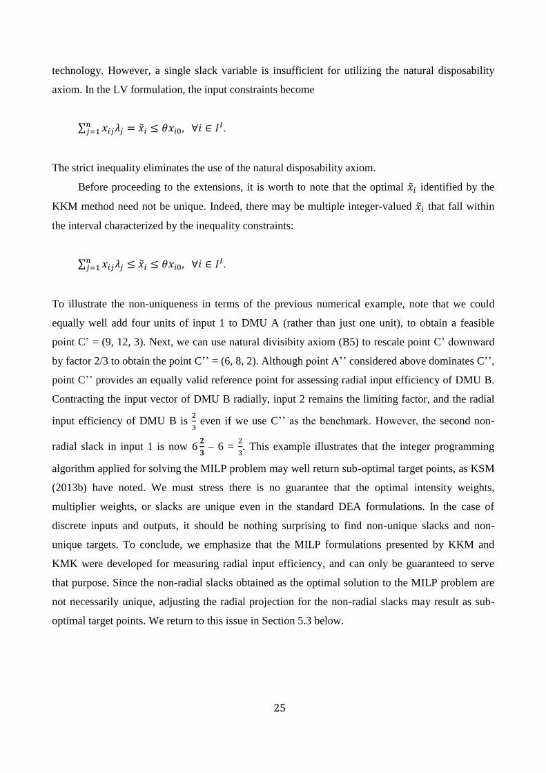
Before proceeding to the extensions, it is worth to note that the optimal identified by the

KKM method need not be unique. Indeed, there may be multiple integer-valued that fall within

the interval characterized by the inequality constraints:

∑ .

To illustrate the non-uniqueness in terms of the previous numerical example, note that we could

equally well add four units of input 1 to DMU A (rather than just one unit), to obtain a feasible

point C’ = (9, 12, 3). Next, we can use natural divisibity axiom (B5) to rescale point C’ downward

by factor 2/3 to obtain the point C’’ = (6, 8, 2). Although point A’’ considered above dominates C’’,

point C’’ provides an equally valid reference point for assessing radial input efficiency of DMU B.

Contracting the input vector of DMU B radially, input 2 remains the limiting factor, and the radial

input efficiency of DMU B is

even if we use C’’ as the benchmark. However, the second non-

radial slack in input 1 is now

– 6 =

. This example illustrates that the integer programming

algorithm applied for solving the MILP problem may well return sub-optimal target points, as KSM

(2013b) have noted. We must stress there is no guarantee that the optimal intensity weights,

multiplier weights, or slacks are unique even in the standard DEA formulations. In the case of

discrete inputs and outputs, it should be nothing surprising to find non-unique slacks and non-

unique targets. To conclude, we emphasize that the MILP formulations presented by KKM and

KMK were developed for measuring radial input efficiency, and can only be guaranteed to serve

that purpose. Since the non-radial slacks obtained as the optimal solution to the MILP problem are

not necessarily unique, adjusting the radial projection for the non-radial slacks may result as sub-

optimal target points. We return to this issue in Section 5.3 below.

26

5. Alternative efficiency metrics

The sound axiomatic foundation of IDEA technology based on the minimum extrapolation principle

makes several extensions of the conventional DEA readily available to IDEA. LV (2007) consider

several alternative efficiency metrics, including the input and output oriented radial Farrell

measures, additive and range-adjusted slack based measures, and the Russell measure. Du et al.

(2012) consider the additive super-efficiency measure in the context of DEA. In this section we

review some alternative efficiency measures, starting from the radial output oriented efficiency

measure, and proceeding to the general directional distance function. We complete this section with

a critical review of additive and slack based measures, noting some problems in these approaches in

the context of IDEA technology.

5.1 Modified Farrell output efficiency measure and its implementation

In Section 4 we restricted attention to the radial input-oriented efficiency measure by Farrell (1957),

modified by KKM to the IDEA context. In this section we briefly extend the discussion to the radial

output measure.

Farrell’s output efficiency measure is defined as

( ) { |( ) }.

Note that in this case = 1 indicates full efficiency, and values indicate that the evaluated

DMU is inefficient (note that we can convert the output efficiency measures to the interval (0, 1] by

using the inverse ). To avoid complications due the discrete nature of IDEA and HIDEA

technologies, we can modify the radial output efficiency measure as:

( ) { | ( ) }.

This modified Farrell measure gauges radial distance to the monotonic hull of the benchmark

technology, requiring that the reference point ( ) must be dominated by a feasible input-

output vector ( ) which has integer-valued inputs for the subset .

The modified output efficiency measure has the usual interpretation of the radial

expansion potential of the evaluated output vector at the given level of inputs. It guarantees that

DMUs assigned the efficiency score one are weakly efficient in the Pareto-Koopmans sense.

27

In the case of the benchmark technology, the modified output efficiency measure

can be computed by solving the following MILP problem:

( )

subject to

{

∑

∑ ,

∑ ,

.

In this case, we indicate the constraints of the integer-valued outputs (subset OI) by curly bracket {.

Note that it is unnecessary to introduce integer-valued input targets

because the inputs are

held constant at their observed levels. This reduces computational complexity compared with the

MILP formulation by LV (2007) because our formulation excludes p integer-valued model

variables as redundant (here p is the number of input factors). Note further that we set two

inequality constraints for the integer-valued outputs to ensure that

∑ .

The first inequality imposes the natural disposability axiom for the integer-valued outputs, whereas

the latter inequality is due to the fact that we measure distance to the monotonic hull of the discrete

HIDEA benchmark technology.

5.2 Modified directional distance function and its implementation

We next consider a modified version of the directional distance function (DDF) by Chambers et al.

(1996, 1998). To our knowledge, this is the first application of DDF to the IDEA context.

DDF allows us to project the observed DMUs to the frontier in non-radial manner, allowing

for simultaneous contraction of inputs and expansion of outputs. DDF indicates the distance from a

given input-output vector to the boundary of the benchmark technology in some pre-assigned

direction ( ) . DDF can be formally defined as

28

( ) { |( ) }.

Note that in this case = 0 indicates full efficiency, and values indicate that the evaluated

DMU is inefficient. Note further that DDF contains the radial input and output efficiency measures

as its special cases. For example, setting ( ) ( ), we obtain

( ) ( ).

To avoid complications due the discrete nature of IDEA and HIDEA technologies, we can

modify the original DDF as:

( )

{ | ( )

( ) ( ) }.

This modified DDF gauges directional distance to the monotonic hull of the benchmark technology,

requiring that the reference point ( ) must be dominated by a feasible input-

output vector ( ) which has integer-valued inputs and outputs for the subsets and .

In the case of the benchmark technology, the modified DDF can be computed by

solving the following MILP problem:

( )

subject to

{

∑

{

∑

∑ ,

∑ .

.

29

In general, DDF requires that we introduce integer-valued targets for both inputs (i.e.,

) and

outputs (

) because DDF can adjust all inputs and outputs simultaneously. However, if the

direction vector ( ) contains any zero elements, we can harmlessly exclude the integer-valued

targets for the corresponding inputs and outputs, and treat those inputs and outputs as fixed factors,

similar to the treatment of outputs in the radial input efficiency measure considered in Section 4.2,

and the treatment of inputs in the radial input efficiency measure considered in Section 5.1.

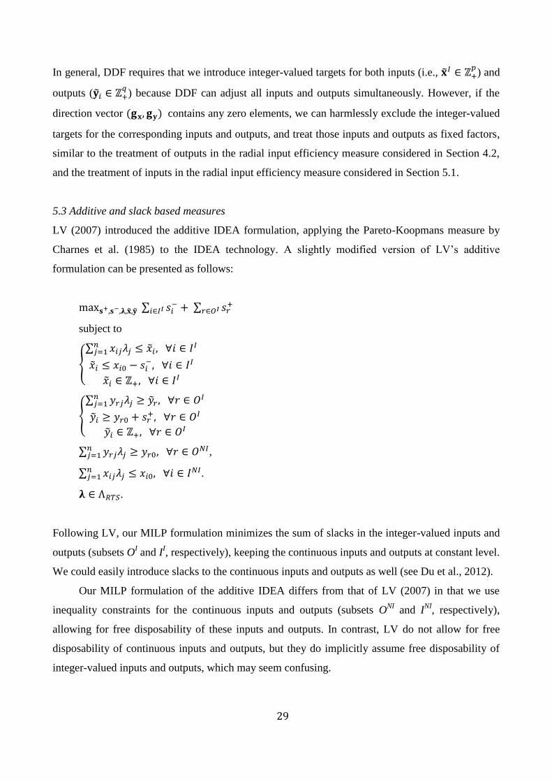
5.3 Additive and slack based measures

LV (2007) introduced the additive IDEA formulation, applying the Pareto-Koopmans measure by

Charnes et al. (1985) to the IDEA technology. A slightly modified version of LV’s additive

formulation can be presented as follows:

∑

∑

subject to

{

∑

{

∑

∑ ,

∑ .

.

Following LV, our MILP formulation minimizes the sum of slacks in the integer-valued inputs and

outputs (subsets OI and I

I, respectively), keeping the continuous inputs and outputs at constant level.

We could easily introduce slacks to the continuous inputs and outputs as well (see Du et al., 2012).

Our MILP formulation of the additive IDEA differs from that of LV (2007) in that we use

inequality constraints for the continuous inputs and outputs (subsets ONI

and INI

, respectively),

allowing for free disposability of these inputs and outputs. In contrast, LV do not allow for free

disposability of continuous inputs and outputs, but they do implicitly assume free disposability of

integer-valued inputs and outputs, which may seem confusing.

30

We noted at the end of Section 4 that the optimal solution of the KKM and KMK MILP

formulations for computing the modified Farrell input efficiency may yield sub-optimal

benchmarks. Specifically, the optimal integer-valued reference point need not be unique, and it is

possible that is dominated by another feasible point. If one is interested in computing efficient

benchmarks, one can first compute the radial or directional projection to the IDEA frontier using the

MILP formulations presented in Sections 4, 5.1, or 5.3, and subsequently apply the additive MILP

formulation presented in this section to maximize the sum of slacks. While the additive formulation

ensures benchmarks that are efficient in the Pareto-Koopmans sense, a unique solution cannot be

guaranteed.

Consider a simple example of three DMUs that use a single integer-valued input x to produce

a single integer-valued output y. Suppose the observed data of DMUs, presented as vectors (x,y) is

the following: A = (2,1), B = (3,2), and C = (3,1). Note that A and B lie on the efficient boundary of

the IDEA technology, whereas C is dominated by both A and B. Now, apply the additive IDEA

formulation to assess efficiency of DMU C. The optimal value of the objective function is unique,

equal to 1. However, neither the benchmark ( ) nor the slacks ( ) are unique. It is possible

to identify DMU A as the benchmark (i.e., ( ) = (2,1)), which yields ( ) = (1,0). It is equally

possible to identify DMU B as the benchmark (i.e., ( ) = (3,2)), which yields ( ) = (0,1).

The MILP algorithm will arbitrarily identify one of these two alternatives to be presented as the

optimal solution. While even standard DEA does not guarantee a unique optimum for the slacks,

benchmarks, or multiplier weights, alternate optima are likely to occur in the context of integer-

valued inputs and outputs. Therefore, it is important to be aware of the fact that the optimal slacks

need not be unique. It seems some of the critiques by KSM are based on misunderstanding this fact.

The additive measure can be used for testing whether the evaluated DMU is on the Pareto-

Koopmans efficient frontier (i.e., ∑

+ ∑

= 0) or not. However, the use of the additive

measure for gauging efficiency is problematic. Non-uniqueness of the optimal slacks noted above is

not the only problem. LV (2007) note that the interpretation of the additive measure as an efficiency

index is meaningful only when the inputs and outputs are measured in the same units of

measurements (e.g., in money), which is not usually the case. Indeed, an appealing feature of DEA

is that inputs and outputs can be measured in different units without a need to convert them to

money metric or other measure of relative values prior to the analysis.

Several attempts to adjust the additive measure to different units of measurement have been

presented in the DEA literature, most notably the range adjusted measure (RAM) by Cooper et al.

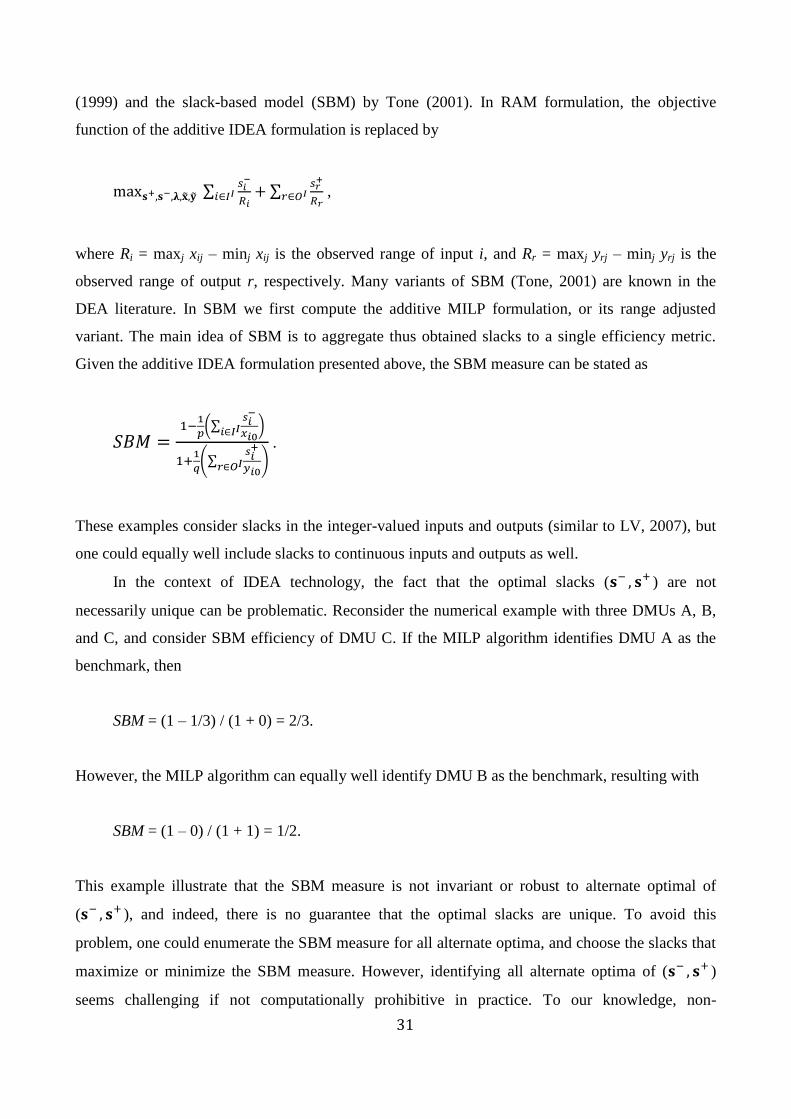
31

(1999) and the slack-based model (SBM) by Tone (2001). In RAM formulation, the objective

function of the additive IDEA formulation is replaced by

∑

∑

,

where Ri = maxj xij – minj xij is the observed range of input i, and Rr = maxj yrj – minj yrj is the

observed range of output r, respectively. Many variants of SBM (Tone, 2001) are known in the

DEA literature. In SBM we first compute the additive MILP formulation, or its range adjusted

variant. The main idea of SBM is to aggregate thus obtained slacks to a single efficiency metric.

Given the additive IDEA formulation presented above, the SBM measure can be stated as

(∑

)

(∑

)

.

These examples consider slacks in the integer-valued inputs and outputs (similar to LV, 2007), but

one could equally well include slacks to continuous inputs and outputs as well.

In the context of IDEA technology, the fact that the optimal slacks ( ) are not

necessarily unique can be problematic. Reconsider the numerical example with three DMUs A, B,

and C, and consider SBM efficiency of DMU C. If the MILP algorithm identifies DMU A as the

benchmark, then

SBM = (1 – 1/3) / (1 + 0) = 2/3.

However, the MILP algorithm can equally well identify DMU B as the benchmark, resulting with

SBM = (1 – 0) / (1 + 1) = 1/2.

This example illustrate that the SBM measure is not invariant or robust to alternate optimal of

( ), and indeed, there is no guarantee that the optimal slacks are unique. To avoid this

problem, one could enumerate the SBM measure for all alternate optima, and choose the slacks that

maximize or minimize the SBM measure. However, identifying all alternate optima of ( )

seems challenging if not computationally prohibitive in practice. To our knowledge, non-

32

uniqueness of slacks and its potential problems have not been duly addressed in the DEA literature.

In our view, non-uniqueness of slacks in DEA is one rational argument for why the radial or

directional distance functions are preferred over the slack based approaches.

We conclude this section by noting that the numerical examples used in this section for

illustrating the non-uniqueness problem may seem overly simplistic. We deliberately used the

simplest thinkable examples to illustrate. If non-uniqueness can occur and cause problems in a

simple example, it would be foolish to assume the problem disappears as one proceeds to more

complex examples or real applications.

6. Stochastic noise

In Section 2.4 we examined the envelopment condition (E1), noting that the best observed

performance level may not be achievable by all DMUs due to unobserved heterogeneity of DMUs

and their operating environments, technological and economic risks and uncertainty, omitted factors

such as quality differences, errors in measurement and data processing, and other sources of noise.

In this section we will briefly extend the StoNED framework introduced by Kuosmanen and

Kortelainen (2012) to the present context of integer valued inputs and outputs.

To maintain direct contact with the conventional stochastic frontier analysis (SFA) and

StoNED, we consider the single-output case, and model the production technology using the

production function f(x), which indicates the maximum output that can be produced with input

vector x (for a general multi-output model, see Section 6.3 in KJS). Thus, the production possibility

set T can be stated as

{( ) | ( ) }.

We do not impose any particular functional form for f: we only assume the production possibility

set T satisfies axiom (A1) for continuous inputs and (B1) for integer-valued inputs, axiom (B2), and

possibly some RTS axioms. Inputs x can be integer-valued or continuous. The main challenge in

this setting concerns the modeling integer-valued output . To our knowledge, all previous

studies on stochastic frontier estimation in the single-output case assume a continuous output

variable.

To model stochastic noise explicitly, the following data generating process will be assumed.

The observed outputs of DMUs i = 1,…,n, denoted as , are assumed to be generated from

equation

33

( ) ,

Where is the input vector of DMU i (which may contain both discrete or continuous inputs), ui is

a random inefficiency term, and vi is a random noise term. Random variables ui and vi are assumed

to be independent of inputs x and of each other. More specific assumptions regarding ui and vi are

the following.

The inefficiency term ui is assumed to be a discrete, Poisson distributed random variable:13

( ),

where parameter ( ) ( ) characterizes both the expected value and variance of the

random inefficiency term (note: should not be confused with the intensity weights of DEA). In

this model, inefficiency is always a non-negative integer, with a known probability mass function

Pr( )

.

Note that a DMU is fully efficient with probability Pr( ) .

The noise term vi is specified as

⌊ ⌋,

where

( ),

and ⌊ ⌋ denotes the largest integer less than or equal to . Parameter ( ) ( )

characterizes both the expected value and variance of the random variable , while ⌊ ⌋ is the

mode of . Note that while random variable is always non-negative, the noise term has zero

13

The Poisson distribution is the most widely used discrete probability distribution in statistics. It can be derived from

the probability of a given number of events occurring in a fixed interval of time and/or space when the events occur

with a known average rate and independently of the time since the last event. Note that the Poisson distribution can be

derived as a limiting case to the binomial distribution as the number of trials approaches to infinity and the expected

number of successes is fixed.

34

mode and it can take either positive and negative values. As parameter increases, the noise term

approaches to the normal distribution with zero mean and variance . Note that in this model the

impact of noise term has the lower bound ⌊ ⌋.

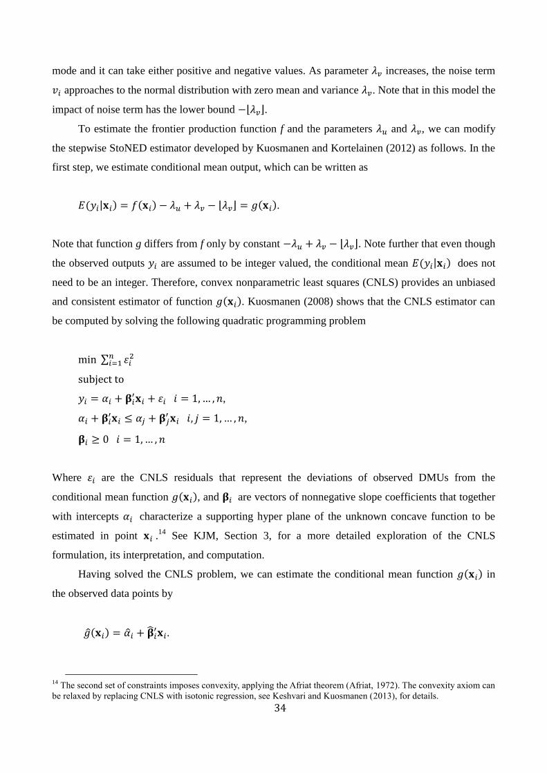
To estimate the frontier production function f and the parameters and , we can modify

the stepwise StoNED estimator developed by Kuosmanen and Kortelainen (2012) as follows. In the

first step, we estimate conditional mean output, which can be written as

( | ) ( ) ⌊ ⌋ ( ).

Note that function g differs from f only by constant ⌊ ⌋. Note further that even though

the observed outputs are assumed to be integer valued, the conditional mean ( | ) does not

need to be an integer. Therefore, convex nonparametric least squares (CNLS) provides an unbiased

and consistent estimator of function ( ). Kuosmanen (2008) shows that the CNLS estimator can

be computed by solving the following quadratic programming problem

∑

,

,

Where are the CNLS residuals that represent the deviations of observed DMUs from the

conditional mean function ( ), and are vectors of nonnegative slope coefficients that together

with intercepts characterize a supporting hyper plane of the unknown concave function to be

estimated in point .14

See KJM, Section 3, for a more detailed exploration of the CNLS

formulation, its interpretation, and computation.

Having solved the CNLS problem, we can estimate the conditional mean function ( ) in

the observed data points by

( ) .

14

The second set of constraints imposes convexity, applying the Afriat theorem (Afriat, 1972). The convexity axiom can

be relaxed by replacing CNLS with isotonic regression, see Keshvari and Kuosmanen (2013), for details.

35

Further, we have the CNLS residuals that are nonparametric estimators of

( ⌊ ⌋) ( ) ( ) ( ) ( ) ( ).

To estimate the parameters and , we can utilize the CNLS residuals and the assumption of

Poisson distributed inefficiency and noise.

Before proceeding to step two, consider random variable . Since is a difference

of two independent Poisson distributed random variables, it follows the Skellam distribution

(Skellam, 1946). The mean, variance and skewness of the Skellam distributed random variable are

related to the central moments of the distribution as follows. Define

, and

( )/2.

Using these notations, the variance and skewness of can be stated as

( ) ,

( ) ( ) .

Note that the CNLS residuals are consistent estimators of minus a constant. Therefore, we can

use the sample variance and skewness of CNLS residuals as estimators of ( ) and ( ), to

obtain estimates and .

Step 2 of the StoNED estimation is the following. Using the above moment equations, we

obtain the following estimators for parameters and :

( ( ) ( )( ( ))

) ,

( ( ) ( )( ( ))

),

Where ( ) and ( ) are the sample variance and skewness of the CNLS residuals,

respectively. Using the parameter estimates and , we can estimate the probability distributions

of inefficiency and noise terms. Recall that expected value of inefficiency is simply , and hence

we can use directly as the estimator of mean inefficiency. Note that in the stochastic frontier

model ( ) is generally expected to be negative. Therefore, negative skewness of residuals

36

increases the mean of the inefficiency term relative to that of the noise term in the Poisson model. If

skewness is zero, then . Positive skewness is also allowed: “wrong skewness” increases the

mean of the noise term compared to that of the inefficiency term. This is an attractive feature of the

Poisson model and the proposed method of moments estimator: wrong skewness does not cause

major problems in this framework.15

In step 3 we adjust the CNLS estimate of the conditional mean ( ) to estimate the frontier.

Note that we need to shift the CNLS estimator upward by the mean inefficiency, but in this case,

also the noise term may have non-zero mean (recall we assumed vi has zero mode, which does not

imply zero mean). Further, we need to take into account that values of the production function must

be integers. Using the equation of the conditional mean ( | ), the integer-valued StoNED

frontier estimator can be stated as

( ) ⌊ ( ) ⌊ ⌋⌋,

where symbol ⌊ ⌋ is denotes the largest integer less than or equal to . Function can be proved to

satisfy the axioms of natural convexity, natural disposability of output and integer-valued inputs,

free disposability of continuous inputs, and any RTS axioms postulated. Function does not

necessarily envelope all observed DMUs, and hence the StoNED frontier will typically lie below

the corresponding IDEA frontier. Note that enveloping noisy data will generally result as biased and

inconsistent estimates. Provided that the assumed doubly-Poisson model of inefficiency and noise is

correctly specified, the StoNED estimator described above can be shown to be statistically

consistent.

To obtain DMU specific efficiency estimates, we must first recognize that the observed

departures from the estimated frontier, that is, ( ) or ( ) , cannot be used directly for

measuring efficiency. We can write the observed distance from the estimated frontier as

( ) ( ( ) ) ( ) ( ( ) ( )) .

Even if our estimate is precise, that is ( ) ( ) , the distance to the estimated frontier

consists of two components: inefficiency and noise. To make DMU specific efficiency assessments,

15

See, e.g., Simar and Wilson (2010) for a more detailed discussion about the wrong skewness problem in stochastic

frontier estimation.

37

we need the conditional distribution of for a given level of ( ), analogous to Jondrow et

al. (1982).

In the discrete case of two Poisson distributed random variables, deriving the conditional

distribution of for given ( ) is relatively straightforward. Firstly, note that we can

calculate the unconditional probabilities ( ) for each , where k denotes the

index of possible values of , and K is the smallest integer that satisfies ( ) for some

pre-specified threshold probability (e.g., we can set 106). Secondly, we know that if ,

then the noise term must be equal to ( ) . Hence, we can calculate the

unconditional probabilities ( ( ) ) associated with each . Note that

if ( ) ⌊ ⌋, then the value of k falls below the minimum bound of noise , and

hence we need to set ( ( ) ) in such cases.

Having calculated the unconditional probability distributions of and for ,

we calculate the sum product

∑ ( ) ( ( ) ) ( ) ⌊ ⌋

.

The conditional distribution of for given ( ) is then obtained as

( | ( )) ( ) ( ( ) )

.

As a point estimator of , one could use the mean of the conditional distribution

( | ( )) ∑ ( | ( )) ,

following the common practice in the SFA literature. Another possibility is to use the median of the

conditional distribution. However, whichever point estimator might be used, it is important to keep

in mind that is essentially a random variable, and hence point estimation of a single realization of

this random variable may be a pointless exercise. We emphasize that the knowledge of the

conditional distribution of at given ( ) provides means for more useful statistical

inferences beyond computing point estimates for efficiency rankings. For example, one could apply

the conditional distributions for assessing the probability that DMU i is more efficient than another

DMU j, or the probability that a group of DMUs is more efficient than another group.

38

While the double-Poisson model and the associated StoNED estimator appear to be well

suited for estimating IDEA technology under noise, one important caveat is worth noting. We

assumed the observed outputs to be non-negative integers, and we would typically assume some

observed to be small, as large integers can be reasonably approximated as continuous variables.

While took the lower bound explicitly into account in the conditional distribution of , we

assumed parameters and to be constant at all input levels. This is not necessarily a realistic

assumption as the range of possible output values typically depends on the input levels, and hence

the variances represented by parameters and are not constant. Therefore, it would be

important to take heteroscedasticity of inefficiency and noise explicitly into account by modeling

these parameters explicitly as functions of inputs, that is, ( ) and ( ). However, we need to

walk before we can run. We leave explicit modeling of heteroscedasticity as an interesting topic for

future research, noting that there exists extensive econometric literature on this topic.16

7. Conclusion and directions for future research

The main insights of this chapter can be classified in three categories. First, a detailed examination

of the axioms of integer DEA and the associated MILP formulations was presented in order to

clarify some points of confusion prevailing in the literature. The key insight gained through this

analysis is the intimate connection between the axioms and the formulation of the MILP problem.

Without a proper understanding of explicitly stated axioms, the MILP formulation will likely

produce erroneous or misleading results. For example, we demonstrated that LV’s MILP

formulations fail to satisfy such axioms as free disposability of continuous inputs and outputs, and

natural divisibility of discrete inputs and outputs. We illustrated through simple numerical examples

that the MILP formulations by LV and KKM yield different results, in contrast to what KSM have

recently claimed. The numerical examples also explain how the differences arise from the

inconsistency of LV’s MILP formulations with their definition of IDEA technology. These

observations underline the critical importance of the sound axiomatic foundation.

Second, we examined alternative efficiency metrics available for integer DEA,

complementing the KKM and KMK formulations for the modified radial input oriented measure

with the modified versions of the radial output oriented measure and the directional distance

function. We also critically discussed the additive efficiency measures, demonstrating by simple

numerical examples that the optimal slacks are not necessarily unique. The non-uniqueness of

16

KJM, Section 8, discusses some of this literature in the context of StoNED estimation.

39

slacks can be particularly problematic for the slack based measures of efficiency in the context of

integer DEA.

Third, we introduced a new model of IDEA technology in the single output setting under

stochastic noise. Modeling both inefficiency and noise as Poisson distributed random variables, we

developed the first extension of the StoNED method to the discrete setting. We developed the

method of moments estimator for identifying the parameters of the double-Poisson model, and

discussed how the conditional distribution of inefficiency at the given distance from the estimated

frontier can be computed and applied for statistical inferences.

In conclusion, we hope that this chapter helps to clarify some issues that have caused

confusion, but also identify some interesting avenues for future research. The basic axioms of DEA

are already well understood in the context of IDEA, but there are other axioms such as weak

disposability (e.g., Kuosmanen, 2005) and selective proportionality (Podinovski, 2004) that deserve

to be examined in the context of IDEA technology. For real applications, probabilistic modeling of

noisy data appears to be the main challenge. In this chapter we presented the first attempt to

modeling stochastic noise in the discrete setting assuming Poisson distributed noise. Further work is

obviously needed to operationalize these ideas to be applicable to real applications. For example,

the truncated distribution of observed outputs above zero and the associated heteroskedasticity

deserve to be addressed explicitly.

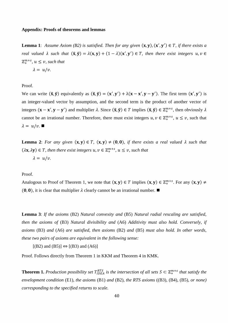
40

Appendix: Proofs of theorems and lemmas

Lemma 1: Assume Axiom (B2) is satisfied. Then for any given ( ) ( ) , if there exists a

real valued such that ( ) ( ) ( )( ) , then there exist integers

, , such that

.

Proof.

We can write ( ) equivalently as ( ) ( ) ( ). The first term ( ) is

an integer-valued vector by assumption, and the second term is the product of another vector of

integers ( ) and multiplier . Since ( ) implies ( ) , then obviously

cannot be an irrational number. Therefore, there must exist integers , , such that

.

Lemma 2: For any given ( ) , ( ) ( ), if there exists a real valued such that

( ) , then there exist integers , , such that

.

Proof.

Analogous to Proof of Theorem 1, we note that ( ) implies ( ) . For any ( )

( ), it is clear that multiplier clearly cannot be an irrational number.

Lemma 3: If the axioms (B2) Natural convexity and (B5) Natural radial rescaling are satisfied,

then the axioms of (B3) Natural divisibility and (A6) Additivity must also hold. Conversely, if

axioms (B3) and (A6) are satisfied, then axioms (B2) and (B5) must also hold. In other words,

these two pairs of axioms are equivalent in the following sense:

[(B2) and (B5)] ⇔ [(B3) and (A6)]

Proof. Follows directly from Theorem 1 in KKM and Theorem 4 in KMK.

Theorem 1. Production possibility set is the intersection of all sets

that satisfy the

envelopment condition (E1), the axioms (B1) and (B2), the RTS axioms ((B3), (B4), (B5), or none)

corresponding to the specified returns to scale.

41

Proof.

See KMK, Theorem 1 (VRS), Theorem 2 (NIRS), Theorem 3 (NDRS), and Theorem 4 (CRS),

proved in Appendix A.

Theorem 2. Production possibility set is the intersection of all sets S that satisfy the

envelopment (E1), axioms (A1) and (A2) for the subsets ( ), axioms (B1) and (B2) for the

subsets ( ), and the RTS axioms ((A3), (A4), (A5), or none for the subsets ( ), and (B3),

(B4), (B5), or none for for the subsets ( )) corresponding to the specified returns to scale.

Proof.

See KMK, Theorem 5 (VRS), Theorem 6 (NIRS), Theorem 7 (NDRS), and Theorem 8 (CRS),

proved in Appendix A.

42

References

Afriat, S.N., 1972. Efficiency Estimation of Production Functions. International Economic Review,

13(3), 568–598.

Aigner, D., Lovell, C.K. and Schmidt, P., 1977. Formulation and estimation of stochastic frontier

production function models. Journal of econometrics, 6, 21–37.

Alirezaee, M.-R., Sani, M.-R.R. 2011. An enumeration algorithm for integer-valued data

envelopment analysis, International Transactions in Operational Research 18(6), 729-740.

Andersen, P. and Petersen, N.C., 1993. A procedure for ranking efficient units in data envelopment

analysis. Management science, 39(10), 1261–1264.

Banker, R.D., Charnes, A. and Cooper, W.W., 1984. Some Models for Estimating Technical and

Scale Inefficiencies in Data Envelopment Analysis. Management Science, 30(9), 1078–1092.

Banker, R.D. and Morey, R.C., 1986. The use of categorical variables in data envelopment analysis.

Management science, 32(12), 1613–1627.

Bogetoft, P., 1994. Incentive efficient production frontiers: an agency perspective on DEA.

Management Science, 40(8), 959–968.

Chambers, R.G., Y.H. Chung, and R. Färe 1996. Benefit and distance functions, Journal of

Economic Theory 70(2), 407-419.

Chambers, R.G., Y.H. Chung, and R. Färe 1998. Profit, directional distance function, and Nerlovian

efficiency, Journal of Optimization Theory and Application 98(2), 351-364.

Charnes, A., W.W. Cooper, B. Golany, L.M. Seiford and J. Stutz 1985. Foundations of data

envelopment analysis for Pareto-Koopmans efficient empirical production functions. Journal

of Econometrics 30(1), 91–107.

Charnes, A., Cooper, W.W. and Rhodes, E., 1978. Measuring the efficiency of decision making

units. European journal of operational research, 2(6), 429–444.

Cherchye, L., Kuosmanen, T. and Post, T., 2001. Alternative treatments of congestion in DEA.

European Journal of Operational Research, 132, 75–80.

Chen, C.-M., Du, J., Huo, J., Zhu, J. 2012. Undesirable factors in integer-valued DEA: Evaluating

the operational efficiencies of city bus systems considering safety records, Decision Support

Systems 54(1), 330-335.

Chen, Y., Djamasbi, S., Du, J., Lim, S., 2013. Integer-valued DEA super-efficiency based on

directional distance function with an application of evaluating mood and its impact on

performance, International Journal of Production Economics 146(2), 550-556.

43

Cooper, W.W., Park, K.S. and Pastor, J.T., 1999. RAM: a range adjusted measure of inefficiency

for use with additive models, and relations to other models and measures in DEA. Journal of

Productivity Analysis, 11, 5–42.

Debreu, G., 1951. The Coefficient of Resource Utilization. Econometrica, 19(3), 273–292.

Deprins, D., Simar, L. and Tulkens, H., 1984. Measuring labor-efficiency in post offices. In M.

Marchand, P. Pestieau, and H. Tulkens, eds. The Performance of Public Enterprises, Concepts

and Measurement. North Holland, Amsterdam: Elsevier Science Ltd.

Du, J., Chen, C.-M., Chen, Y., Cook, W.D., Zhu, J. 2012. Additive super-efficiency in integer-

valued data envelopment analysis. European Journal of Operational Research, 218(1), 186–

192.

Farrell, M., 1957. The measurement of productive efficiency. Journal of the Royal Statistical

Society, Series A, 120(3), 253–290.

Färe, R. and Grosskopf, S., 2009. A Comment on Weak Disposability in Nonparametric Production

Analysis. American Journal of Agricultural Economics, 91(2), 535–538.

Jondrow, J., C.A.K. Lovell, I.S. Materov, and P. Schmidt 1982. On estimation of technical

inefficiency in the stochastic frontier production function model, Journal of Econometrics 19,

233-238.

Kamakura, W.A., 1988. A Note on “The Use of Categorical Variables in Data Envelopment

Analysis”. Management science 34(10), 1273–1276.

Kazemi Matin, R., Emrouznejad, A. 2011. An integer-valued data envelopment analysis model with

bounded outputs, International Transactions in Operational Research 18(6), 741-749.

Kazemi Matin, R. and Kuosmanen, T., 2009. Theory of integer-valued data envelopment analysis

under alternative returns to scale axioms. Omega, 37(5), 988–995.

Keshvari, A. and Kuosmanen, T., 2013. Stochastic non-convex envelopment of data: Applying

isotonic regression to frontier estimation. European Journal of Operational Research, 231(2),

481–491.

Khezrimotlagh, D., Salleh, S. and Mohsenpour, Z., 2012. A Comment on Theory of Integer-Valued

Data Envelopment Analysis. Applied Mathematical Sciences, 6(116), 5769–5774.

Khezrimotlagh, D., Salleh, S. and Mohsenpour, Z., 2013a. A new robust mixed integer-valued

model in DEA. Applied Mathematical Modelling, 37(24), 9885–9897.

Khezrimotlagh, D., Salleh, S., Mohsenpour, Z. 2013b. A note on integer-valued radial model in

DEA, Computers and Industrial Engineering 66(1), 199-200.

44

Koopmans, T.C., 1951. Analysis of production as an efficient combination of activities. In T. C.

Koopmans, ed. Activity analysis of production and allocation. New York: John Wiley and

Sons, Inc., 33–97.

Koopmans, T.C. (Ed.) 1951. Activity analysis of production and allocation, Cowles Commission

for Research in Economics, John Wiley & Sons, Inc., New York.

Kuosmanen, T. 2001. DEA with Efficiency Classification Preserving Conditional Convexity,

European Journal of Operational Research 132(2), 326-342.

Kuosmanen, T. 2003. Duality Theory of Non-convex Technologies, Journal of Productivity

Analysis 20, 273-304.

Kuosmanen, T., 2005. Weak disposability in nonparametric production analysis with undesirable

outputs. American Journal of Agricultural Economics, 87(November), 1077–1082.

Kuosmanen, T. (2008): Representation Theorem for Convex Nonparametric Least Squares,

Econometrics Journal 11, 308-325.

Kuosmanen, T., and A.L. Johnson 2010. Data Envelopment Analysis as Nonparametric Least

Squares Regression, Operations Research 58(1): 149-160.

Kuosmanen, T., A.L. Johnson, and A. Saastamoinen (2014) Stochastic nonparametric approach to

efficiency analysis: A unified framework, in J. Zhu (Eds) Handbook on Data Envelopment

Analysis Vol II, Springer.

Kuosmanen, T. and Kazemi Matin, R., 2009. Theory of integer-valued data envelopment analysis.

European Journal of Operational Research, 192(2), 658–667.

Kuosmanen, T., and M. Kortelainen (2012): Stochastic Non-Smooth Envelopment of Data: Semi-

Parametric Frontier Estimation Subject to Shape Constraints, Journal of Productivity Analysis

38(1), 11-28.

Kuosmanen, T. and Podinovski, V. V., 2009. Weak Disposability in Nonparametric Production

Analysis: Reply to Färe and Grosskopf. American Journal of Agricultural Economics, 91(2),

539–545.

Kuosmanen, T., G.T. Post and T. Sipiläinen 2004. Shadow Price Approach to Total Factor

Productivity Measurement: With an Application to Finnish Grass-Silage Production, Journal

of Productivity Analysis 22(1), 95-121.

Lozano, S. 2013. Using DEA to find the best partner for a horizontal cooperation, Computers and

Industrial Engineering 66(2), 286-292.

Lozano, S. and Villa, G., 2006. Data envelopment analysis of integer-valued inputs and outputs.

Computers and Operations Research, 33(10), 3004–3014.

45

Lozano, S. and Villa, G., 2007. Integer DEA models. In J. Zhu and W. D. Cook, eds. Modeling

Data Irregularities and Structural Complexities in Data Envelopment Analysis. New York:

Springer, 271–290.

Lozano, S., Villa, G., Canca, D. 2011. Application of centralised DEA approach to capital

budgeting in Spanish ports, Computers and Industrial Engineering 60(3), 455-465.

Meeusen, W. and Vanden Broeck, J., 1977. Efficiency estimation from Cobb-Douglas production

functions with composed error. International economic review, 18(2), 435–444.

Nöhren, M., Heinzl, A. 2012. Measuring the relative efficiency of global delivery models in IT

outsourcing, Lecture Notes in Business Information Processing 130, 61-75.

Pareto, V., 1909. Manuel d’Economie politique, Paris: V. Giard et E. Brière.

Podinovski, V. V., 2004. Bridging the gap between the constant and variable returns-to-scale

models: selective proportionality in data envelopment analysis. Journal of the Operational

Research Society, 55(3), 265–276.

Post, G.T., 2001. Transconcave data envelopment analysis, European Journal of Operational

Research 132(2), 374-389.

Rousseau, J.J. and Semple, J.H., 1993. Notes : Categorical Outputs Data Envelopment Analysis. ,

39(3), 384–386.

Shephard, R., 1970. Theory of Cost and Production Functions, Princeton: Princeton University

Press.

Simar, L., and P.W. Wilson 2010. Inferences from cross-sectional, stochastic frontier models.

Econometric Reviews 29(1), 62-98.

Skellam, J.G. 1946. The frequency distribution of the difference between two Poisson variates

belonging to different populations, Journal of the Royal Statistical Society Series A, 109(3),

296-296.

Tone, K., 2001. A slacks-based measure of efficiency in data envelopment analysis. European

Journal of Operational Research, 130, 498–509.

Tulkens, H., 1993. On FDH efficiency analysis: Some methodological issues and applications to

retail banking, courts, and urban transit. Journal of Productivity Analysis, 4, 183–210.

Von Neumann, J., 1945-1946. A Model of General Economic Equilibrium, Review of Economic

Studies 13(1), 1-9.

Wang, Y., S. Wang, C. Dang, and W. Ge 2014. Nonparametric quantile frontier estimation under

shape restriction. European Journal of Operational Research, 232(3), 671–678.

46

Wu, J., Zhou, Z. and Liang, L., 2009. Measuring the Performance of Nations at Beijing Summer

Olympics Using Integer-Valued DEA Model. Journal of Sports Economics, 11(5), 549–566.

Wu, J., Liang, L., Song, H. 2010. Measuring hotel performance using the integer DEA model,

Tourism Economics 16(4), 867-882.