Proceedings of the 2011 Conference on Empirical Methods in Natural Language Processing, pages 616–627,Edinburgh, Scotland, UK, July 27–31, 2011. c©2011 Association for Computational Linguistics

Discovering Morphological Paradigms from Plain TextUsing a Dirichlet Process Mixture Model

Markus Dreyer∗SDL Language Weaver

Los Angeles, CA 90045, USAmdreyer@sdl.com

Jason EisnerComputer Science Dept., Johns Hopkins University

Baltimore, MD 21218, USAjason@cs.jhu.edu

Abstract

We present an inference algorithm that orga-nizes observed words (tokens) into structuredinflectional paradigms (types). It also natu-rally predicts the spelling of unobserved formsthat are missing from these paradigms, and dis-covers inflectional principles (grammar) thatgeneralize to wholly unobserved words.

Our Bayesian generative model of the data ex-plicitly represents tokens, types, inflections,paradigms, and locally conditioned string edits.It assumes that inflected word tokens are gen-erated from an infinite mixture of inflectionalparadigms (string tuples). Each paradigm issampled all at once from a graphical model,whose potential functions are weighted finite-state transducers with language-specific param-eters to be learned. These assumptions natu-rally lead to an elegant empirical Bayes infer-ence procedure that exploits Monte Carlo EM,belief propagation, and dynamic programming.Given 50–100 seed paradigms, adding a 10-million-word corpus reduces prediction errorfor morphological inflections by up to 10%.

1 Introduction1.1 Motivation

Statistical NLP can be difficult for morphologicallyrich languages. Morphological transformations onwords increase the size of the observed vocabulary,which unfortunately masks important generalizations.In Polish, for example, each lexical verb has literally100 inflected forms (Janecki, 2000). That is, a singlelexeme may be realized in a corpus as many differentword types, which are differently inflected for person,number, gender, tense, mood, etc.

∗ This research was done at Johns Hopkins University aspart of the first author’s dissertation work. It was supported bythe Human Language Technology Center of Excellence and bythe National Science Foundation under Grant No. 0347822.

All this makes lexical features even sparser thanthey would be otherwise. In machine translationor text generation, it is difficult to learn separatelyhow to translate, or when to generate, each of thesemany word types. In text analysis, it is difficult tolearn lexical features (as cues to predict topic, syntax,semantics, or the next word), because one must learna separate feature for each word form, rather thangeneralizing across inflections.

Our engineering goal is to address these problemsby mostly-unsupervised learning of morphology. Ourlinguistic goal is to build a generative probabilisticmodel that directly captures the basic representationsand relationships assumed by morphologists. Thismodel suffices to define a posterior distribution overanalyses of any given collection of type and/or tokendata. Thus we obtain scientific data interpretation asprobabilistic inference (Jaynes, 2003). Our computa-tional goal is to estimate this posterior distribution.

1.2 What is EstimatedOur inference algorithm jointly reconstructs token,type, and grammar information about a language’smorphology. This has not previously been attempted.

Tokens: We will tag each word token in a corpuswith (1) a part-of-speech (POS) tag,1 (2) an inflection,and (3) a lexeme. A token of brokenmight be taggedas (1) a VERB and more specifically as (2) the pastparticiple inflection of (3) the abstract lexeme �b&r��a�k.2

Reconstructing the latent lexemes and inflectionsallows the features of other statistical models to con-sider them. A parser may care that broken is apast participle; a search engine or question answer-ing system may care that it is a form of �b&r��a�k; and atranslation system may care about both facts.

1POS tagging may be done as part of our Bayesian model orbeforehand, as a preprocessing step. Our experiments chose thelatter option, and then analyzed only the verbs (see section 8).

2We use cursive font for abstract lexemes to emphasize thatthey are atomic objects that do not decompose into letters.

616

singular pluralpresent 1st-person breche brechen

2nd-person brichst brecht3rd-person bricht brechen

past 1st-person brach brachen2nd-person brachst bracht3rd-person brach brachen

Table 1: Part of a morphological paradigm in German,showing the spellings of some inflections of the lexeme�b&r��a�k (whose lemma is brechen), organized in a grid.

Types: In carrying out the above, we will recon-struct specific morphological paradigms of the lan-guage. A paradigm is a grid of all the inflected formsof some lexeme, as illustrated in Table 1. Our recon-structed paradigms will include our predictions ofinflected forms that were never observed in the cor-pus. This tabular information about the types (ratherthan the tokens) of the language may be separatelyuseful, for example in translation and other genera-tion tasks, and we will evaluate its accuracy.

Grammar: We estimate parameters ~θ that de-scribe general patterns in the language. We learna prior distribution over inflectional paradigms bylearning (e.g.) how a verb’s suffix or stem voweltends to change when it is pluralized. We also learn(e.g.) whether singular or plural forms are more com-mon. Our basic strategy is Monte Carlo EM, so theseparameters tell us how to guess the paradigms (MonteCarlo E step), then these reconstructed paradigms tellus how to reestimate the parameters (M step), and soon iteratively. We use a few supervised paradigms toinitialize the parameters and help reestimate them.

2 Overview of the Model

We begin by sketching the main ideas of our model,first reviewing components that we introduced inearlier papers. Sections 5–7 will give more formaldetails. Full details and more discussion can be foundin the first author’s dissertation (Dreyer, 2011).

2.1 Modeling Morphological Alternations

We begin with a family of joint distributions p(x, y)over string pairs, parameterized by ~θ. For example,to model just the semi-systematic relation between aGerman lemma and its 3rd-person singular presentform, one could train ~θ to maximize the likelihoodof (x, y) pairs such as (brechen, bricht). Then,given a lemma x, one could predict its inflected form

y via p(y | x), and vice-versa.Dreyer et al. (2008) define such a family via a

log-linear model with latent alignments,

p(x, y) =∑

a

p(x, y, a) ∝∑

a

exp(~θ · ~f(x, y, a))

Here a ranges over monotonic 1-to-1 character align-ments between x and y. ∝means “proportional to” (pis normalized to sum to 1). ~f extracts a vector of localfeatures from the aligned pair by examining trigramwindows. Thus ~θ can reward or penalize specificfeatures—e.g., insertions, deletions, or substitutionsin specific contexts, as well as trigram features of xand y separately.3 Inference and training are done bydynamic programming on finite-state transducers.

2.2 Modeling Morphological ParadigmsA paradigm such as Table 1 describes how some ab-stract lexeme (�b&r��a�k) is expressed in German.4 Weevaluate whole paradigms as linguistic objects, fol-lowing word-and-paradigm or realizational morphol-ogy (Matthews, 1972; Stump, 2001). That is, we pre-sume that some language-specific distribution p(π)defines whether a paradigm π is a grammatical—anda priori likely—way for a lexeme to express itselfin the language. Learning p(π) helps us reconstructparadigms, as described at the end of section 1.2.

Let π = (x1, x2, . . .). In Dreyer and Eisner (2009),we showed how to model p(π) as a renormalizedproduct of many pairwise distributions prs(xr, xs),each having the log-linear form of section 2.1:

p(π) ∝∏

r,s

prs(xr, xs) ∝ exp(∑

r,s

~θ·−→frs(xr, xs, ars))

This is an undirected graphical model (MRF) overstring-valued random variables xs; each factor prsevaluates the relationship between some pair ofstrings. Note that it is still a log-linear model, and pa-rameters in ~θ can be reused across different rs pairs.

To guess at unknown strings in the paradigm,Dreyer and Eisner (2009) show how to perform ap-proximate inference on such an MRF by loopy belief

3Dreyer et al. (2008) devise additional helpful features basedon enriching the aligned pair with additional latent information,but our present experiments drop those for speed.

4Our present experiments focus on orthographic forms, be-cause we are learning from a written corpus. But it would benatural to use phonological forms instead, or to include both inthe paradigm so as to model their interrelationships.

617

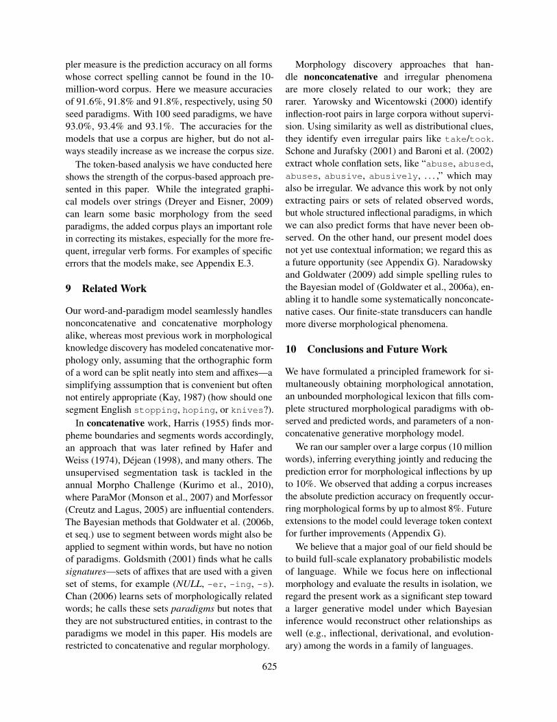
X1pl

X2pl

X3pl

XLem

X1sg

X2sg

X3sg

brichenbrechen ... ? brichen

brechen ... ?

brichtbrecht ... ?

brichebreche ... ?

brichstbrechst ... ?

bricht brechen

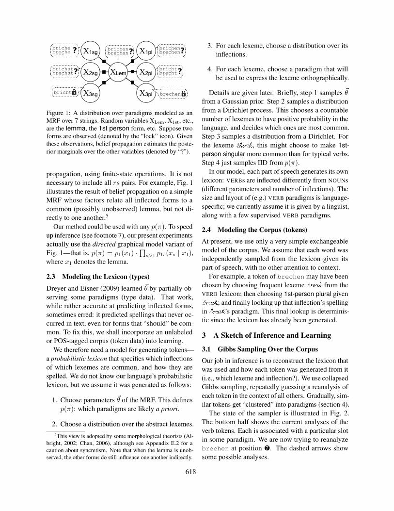
Figure 1: A distribution over paradigms modeled as anMRF over 7 strings. Random variables XLem, X1st, etc.,are the lemma, the 1st person form, etc. Suppose twoforms are observed (denoted by the “lock” icon). Giventhese observations, belief propagation estimates the poste-rior marginals over the other variables (denoted by “?”).

propagation, using finite-state operations. It is notnecessary to include all rs pairs. For example, Fig. 1illustrates the result of belief propagation on a simpleMRF whose factors relate all inflected forms to acommon (possibly unobserved) lemma, but not di-rectly to one another.5

Our method could be used with any p(π). To speedup inference (see footnote 7), our present experimentsactually use the directed graphical model variant ofFig. 1—that is, p(π) = p1(x1) ·

∏s>1 p1s(xs | x1),

where x1 denotes the lemma.

2.3 Modeling the Lexicon (types)

Dreyer and Eisner (2009) learned ~θ by partially ob-serving some paradigms (type data). That work,while rather accurate at predicting inflected forms,sometimes erred: it predicted spellings that never oc-curred in text, even for forms that “should” be com-mon. To fix this, we shall incorporate an unlabeledor POS-tagged corpus (token data) into learning.

We therefore need a model for generating tokens—a probabilistic lexicon that specifies which inflectionsof which lexemes are common, and how they arespelled. We do not know our language’s probabilisticlexicon, but we assume it was generated as follows:

1. Choose parameters ~θ of the MRF. This definesp(π): which paradigms are likely a priori.

2. Choose a distribution over the abstract lexemes.5This view is adopted by some morphological theorists (Al-

bright, 2002; Chan, 2006), although see Appendix E.2 for acaution about syncretism. Note that when the lemma is unob-served, the other forms do still influence one another indirectly.

3. For each lexeme, choose a distribution over itsinflections.

4. For each lexeme, choose a paradigm that willbe used to express the lexeme orthographically.

Details are given later. Briefly, step 1 samples ~θfrom a Gaussian prior. Step 2 samples a distributionfrom a Dirichlet process. This chooses a countablenumber of lexemes to have positive probability in thelanguage, and decides which ones are most common.Step 3 samples a distribution from a Dirichlet. Forthe lexeme �t�h�i�n�k, this might choose to make 1st-person singular more common than for typical verbs.Step 4 just samples IID from p(π).

In our model, each part of speech generates its ownlexicon: VERBs are inflected differently from NOUNs(different parameters and number of inflections). Thesize and layout of (e.g.) VERB paradigms is language-specific; we currently assume it is given by a linguist,along with a few supervised VERB paradigms.

2.4 Modeling the Corpus (tokens)At present, we use only a very simple exchangeablemodel of the corpus. We assume that each word wasindependently sampled from the lexicon given itspart of speech, with no other attention to context.

For example, a token of brechen may have beenchosen by choosing frequent lexeme �b&r��a�k from theVERB lexicon; then choosing 1st-person plural given�b&r��a�k; and finally looking up that inflection’s spellingin �b&r��a�k’s paradigm. This final lookup is determinis-tic since the lexicon has already been generated.

3 A Sketch of Inference and Learning

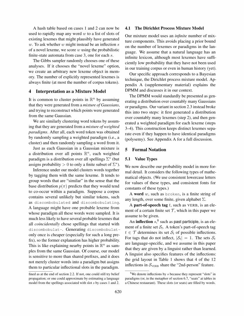
3.1 Gibbs Sampling Over the CorpusOur job in inference is to reconstruct the lexicon thatwas used and how each token was generated from it(i.e., which lexeme and inflection?). We use collapsedGibbs sampling, repeatedly guessing a reanalysis ofeach token in the context of all others. Gradually, sim-ilar tokens get “clustered” into paradigms (section 4).

The state of the sampler is illustrated in Fig. 2.The bottom half shows the current analyses of theverb tokens. Each is associated with a particular slotin some paradigm. We are now trying to reanalyzebrechen at position ¼. The dashed arrows showsome possible analyses.

618

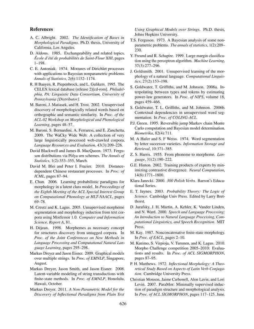
singular plural

1st

2nd

3rd bricht

brichstbrechst... ?

brichebreche... ?

brechen

brichtbrecht... ?

brichenbrechen... ?

springstsprengst... ?

springesprenge... ?

springtsprengt... ?

springensprengen...

springensprengen...

1 3

Index i 2PRON

4NOUN

6PREPPOS ti

Infl si

Spell wi

Lex �i

1VERB

3rd sg.bricht

5VERB

2nd pl.springt

3VERB

3rd pl.brechen

??

5

Lexicon

Corpus

?

...

?

?

springt

7VERB

1st pl.

...brechen... ... ...

3rd pl.

Figure 2: A state of the Gibbs sampler (note that theassumed generative process runs roughly top-to-bottom).Each corpus token i has been tagged with part of speech ti,lexeme `i and inflection si. Token ¶ has been tagged as�b&r��a�k and 3rd sg., which locked the corresponding typespelling in the paradigm to the spelling w1 = bricht;similarly for ¸ and º. Now w7 is about to be reanalyzed.

The key intuition is that the current analyses of theother verb tokens imply a posterior distribution overthe VERB lexicon, shown in the top half of the figure.

First, because of the current analyses of ¶ and ¸,the 3rd-person spellings of �b&r��a�k are already con-strained to match w1 and w3 (the “lock” icon).

Second, belief propagation as in Fig. 1 tells uswhich other inflections of �b&r��a�k (the “?” icon) areplausibly spelled as brechen, and how likely theyare to be spelled that way.

Finally, the fact that other tokens are associatedwith �b&r��a�k suggest that this is a popular lexeme, mak-ing it a plausible explanation of ¼ as well. (This isthe “rich get richer” property of the Chinese restau-rant process; see section 6.6.) Furthermore, certaininflections of �b&r��a�k appear to be especially popular.

In short, given the other analyses, we know whichinflected lexemes in the lexicon are likely, and howlikely each one is to be spelled as brechen. This letsus compute the relative probabilities of the possibleanalyses of token ¼, so that the Gibbs sampler canaccordingly choose one of these analyses at random.

3.2 Monte Carlo EM Training of ~θ

For a given ~θ, this Gibbs sampler converges to theposterior distribution over analyses of the full corpus.To improve our ~θ estimate, we periodically adjust ~θto maximize or increase the probability of the mostrecent sample(s). For example, having tagged w5 =

springt as s5 = 2nd-person plural may strengthenour estimated probability that 2nd-person spellingstend to end in -t. That revision to ~θ, in turn, willinfluence future moves of the sampler.

If the sampler is run long enough between calls tothe ~θ optimizer, this is a Monte Carlo EM procedure(see end of section 1.2). It uses the data to optimize alanguage-specific prior p(π) over paradigms—an em-pirical Bayes approach. (A fully Bayesian approachwould resample ~θ as part of the Gibbs sampler.)

3.3 Collapsed Representation of the Lexicon

The lexicon is collapsed out of our sampler, in thesense that we do not represent a single guess about theinfinitely many lexeme probabilities and paradigms.What we store about the lexicon is information aboutits full posterior distribution: the top half of Fig. 2.

Fig. 2 names its lexemes as �b&r��a�k and �j�u�m�p for ex-pository purposes, but of course the sampler cannotreconstruct such labels. Formally, these labels are col-lapsed out, and we represent lexemes as anonymousobjects. Tokens ¶ and ¸ are tagged with the sameanonymous lexeme (which will correspond to sittingat the same table in a Chinese restaurant process).

For each lexeme ` and inflection s, we maintainpointers to any tokens currently tagged with the slot(`, s). We also maintain an approximate marginaldistribution over the spelling of that slot:6

1. If (`, s) points to at least one token i, then weknow (`, s) is spelled as wi (with probability 1).

2. Otherwise, the spelling of (`, s) is not known.But if some spellings in `’s paradigm are known,store a truncated distribution that enumerates the25 most likely spellings for (`, s), according toloopy belief propagation within the paradigm.

3. Otherwise, we have observed nothing about `:it is currently unused. All such ` share the samemarginal distribution over spellings of (`, s):the marginal of the prior p(π). Here a 25-bestlist could not cover all plausible spellings. In-stead we store a probabilistic finite-state lan-guage model that approximates this marginal.7

6Cases 1 and 2 below must in general be updated whenevera slot switches between having 0 and more than 0 tokens. Cases2 and 3 must be updated when the parameters ~θ change.

7This character trigram model is fast to build if p(π) is de-

619

A hash table based on cases 1 and 2 can now beused to rapidly map any word w to a list of slots ofexisting lexemes that might plausibly have generatedw. To ask whether w might instead be an inflection sof a novel lexeme, we score w using the probabilisticfinite-state automata from case 3, one for each s.

The Gibbs sampler randomly chooses one of theseanalyses. If it chooses the “novel lexeme” option,we create an arbitrary new lexeme object in mem-ory. The number of explicitly represented lexemes isalways finite (at most the number of corpus tokens).

4 Interpretation as a Mixture Model

It is common to cluster points in Rn by assumingthat they were generated from a mixture of Gaussians,and trying to reconstruct which points were generatedfrom the same Gaussian.

We are similarly clustering word tokens by assum-ing that they are generated from a mixture of weightedparadigms. After all, each word token was obtainedby randomly sampling a weighted paradigm (i.e., acluster) and then randomly sampling a word from it.

Just as each Gaussian in a Gaussian mixture isa distribution over all points Rn, each weightedparadigm is a distribution over all spellings Σ∗ (butassigns probability > 0 to only a finite subset of Σ∗).

Inference under our model clusters words togetherby tagging them with the same lexeme. It tends togroup words that are “similar” in the sense that thebase distribution p(π) predicts that they would tendto co-occur within a paradigm. Suppose a corpuscontains several unlikely but similar tokens, suchas discombobulated and discombobulating.A language might have one probable lexeme fromwhose paradigm all these words were sampled. It ismuch less likely to have several probable lexemes thatall coincidentally chose spellings that started withdiscombobulat-. Generating discombobulat-

only once is cheaper (especially for such a long pre-fix), so the former explanation has higher probability.This is like explaining nearby points in Rn as sam-ples from the same Gaussian. Of course, our modelis sensitive to more than shared prefixes, and it doesnot merely cluster words into a paradigm but assignsthem to particular inflectional slots in the paradigm.fined as at the end of section 2.2. If not, one could still try beliefpropagation; or one could approximate by estimating a languagemodel from the spellings associated with slot s by cases 1 and 2.

4.1 The Dirichlet Process Mixture Model

Our mixture model uses an infinite number of mix-ture components. This avoids placing a prior boundon the number of lexemes or paradigms in the lan-guage. We assume that a natural language has aninfinite lexicon, although most lexemes have suffi-ciently low probability that they have not been usedin our training corpus or even in human history (yet).

Our specific approach corresponds to a Bayesiantechnique, the Dirichlet process mixture model. Ap-pendix A (supplementary material) explains theDPMM and discusses it in our context.

The DPMM would standardly be presented as gen-erating a distribution over countably many Gaussiansor paradigms. Our variant in section 2.3 instead brokethis into two steps: it first generated a distributionover countably many lexemes (step 2), and then gen-erated a weighted paradigm for each lexeme (steps3–4). This construction keeps distinct lexemes sepa-rate even if they happen to have identical paradigms(polysemy). See Appendix A for a full discussion.

5 Formal Notation

5.1 Value Types

We now describe our probability model in more for-mal detail. It considers the following types of mathe-matical objects. (We use consistent lowercase lettersfor values of these types, and consistent fonts forconstants of these types.)

A word w, such as broken, is a finite string ofany length, over some finite, given alphabet Σ.

A part-of-speech tag t, such as VERB, is an ele-ment of a certain finite set T , which in this paper weassume to be given.

An inflection s,8 such as past participle, is an ele-ment of a finite set St. A token’s part-of-speech tagt ∈ T determines its set St of possible inflections.For tags that do not inflect, |St| = 1. The sets Stare language-specific, and we assume in this paperthat they are given by a linguist rather than learned.A linguist also specifies features of the inflections:the grid layout in Table 1 shows that 4 of the 12inflections in SVERB share the “2nd-person” feature.

8We denote inflections by s because they represent “slots” inparadigms (or, in the metaphor of section 6.7, “seats” at tables ina Chinese restaurant). These slots (or seats) are filled by words.

620

A paradigm for t ∈ T is a mapping π : St → Σ∗,specifying a spelling for each inflection in St. Table 1shows one VERB paradigm.

A lexeme ` is an abstract element of some lexicalspace L. Lexemes have no internal semantic struc-ture: the only question we can ask about a lexeme iswhether it is equal to some other lexeme. There is noupper bound on how many lexemes can be discoveredin a text corpus; L is infinite.

5.2 Random Quantities

Our generative model of the corpus is a joint probabil-ity distribution over a collection of random variables.We describe them in the same order as section 1.2.

Tokens: The corpus is represented by token vari-ables. In our setting the sequence of words ~w =w1, . . . , wn ∈ Σ∗ is observed, along with n. Wemust recover the corresponding part-of-speech tags~t = t1, . . . , tn ∈ T , lexemes ~̀ = `1, . . . , `n ∈ L,and inflections ~s = s1, . . . , sn, where (∀i)si ∈ Sti .

Types: The lexicon is represented by typevariables. For each of the infinitely many lex-emes ` ∈ L, and each t ∈ T , the paradigmπt,` is a function St → Σ∗. For example,Table 1 shows a possible value πVERB,�b&r��a�k.The various spellings in the paradigm, such asπVERB,�b&r��a�k(1st-person sing. pres.)=breche, arestring-valued random variables that are correlatedwith one another.

Since the lexicon is to be probabilistic (section 2.3),Gt(`) denotes tag t’s distribution over lexemes ` ∈L, while Ht,`(s) denotes the tagged lexeme (t, `)’sdistribution over inflections s ∈ St.

Grammar: Global properties of the language arecaptured by grammar variables that cut across lex-ical entries: our parameters ~θ that describe typicalinflectional alternations, plus parameters ~φt, αt, α′t, ~τ(explained below). Their values control the overallshape of the probabilistic lexicon that is generated.

6 The Formal Generative Model

We now fully describe the generative process thatwas sketched in section 2. Step by step, it randomlychooses an assignment to all the random variables ofsection 5.2. Thus, a given assignment’s probability—which section 3’s algorithms consult in order to re-sample or improve the current assignment—is the

product of the probabilities of the individual choices,as described in the sections below. (Appendix Bprovides a drawing of this as a graphical model.)

6.1 Grammar Variables p(~θ), p(−→φt), p(αt), p(α′t)First select the grammar variables from a prior. (Wewill see below how these variables get used.) Ourexperiments used fairly flat priors. Each weight in ~θor−→φt is drawn IID from N (0, 10), and each αt or α′t

from a Gamma with mode 10 and variance 1000.

6.2 Paradigms p(πt,` | ~θ)For each t ∈ T , let Dt(π) denote the distributionover paradigms that was presented in section 2.2(where it was called p(π)). Dt is fully specified byour graphical model for paradigms of part of speecht, together with its parameters ~θ as generated above.

This is the linguistic core of our model. It consid-ers spellings: DVERB describes what verb paradigmstypically look like in the language (e.g., Table 1).

Parameters in ~θ may be shared across parts ofspeech t. These “backoff” parameters capture gen-eral phonotactics of the language, such as prohibitedletter bigrams or plausible vowel changes.

For each possible tagged lexeme (t, `), we nowdraw a paradigm πt,` fromDt. Most of these lexemeswill end up having probability 0 in the language.

6.3 Lexical Distributions p(Gt | αt)We now formalize section 2.3. For each t ∈ T , thelanguage has a distribution Gt(`) over lexemes. Wedraw Gt from a Dirichlet process DP(G,αt), whereG is the base distribution over L, and αt > 0 isa concentration parameter generated above. If αtis small, then Gt will tend to have the property thatmost of its probability mass falls on relatively fewof the lexemes in Lt def

= {` ∈ L : Gt(`) > 0}. Aclosed-class tag is one whose αt is especially small.

For G to be a uniform distribution over an infinitelexeme set L, we need L to be uncountable.9 How-ever, it turns out10 that with probability 1, each Ltis countably infinite, and all the Lt are disjoint. Soeach lexeme ` ∈ L is selected by at most one tag t.

9For example, L def= [0, 1], so that �b&r��a�k is merely a sugges-

tive nickname for a lexeme such as 0.2538159.10This can be seen by considering the stick-breaking construc-

tion of the Dirichlet process that (Sethuraman, 1994; Teh et al.,2006). A separate stick is broken for each Gt. See Appendix A.

621

6.4 Inflectional Distributions p(Ht,` |−→φt, α′t)

For each tagged lexeme (t, `), the language specifiessome distribution Ht,` over its inflections.

First we construct backoff distributions Ht that areindependent of `. For each tag t ∈ T , let Ht be somebase distribution over St. As St could be large insome languages, we exploit its grid structure (Table 1)to reduce the number of parameters of Ht. We takeHt to be a log-linear distribution with parameters

−→φt

that refer to features of inflections. E.g., the 2nd-person inflections might be systematically rare.

Now we model each Ht,` as an independent drawfrom a finite-dimensional Dirichlet distribution withmeanHt and concentration parameter α′t. E.g., �t�h�i�n�kmight be biased toward 1st-person sing. present.

6.5 Part-of-Speech Tag Sequence p(~t | ~τ)

In our current experiments, ~t is given. But in general,to discover tags and inflections simultaneously, wecan suppose that the tag sequence ~t (and its length n)are generated by a Markov model, with tag bigram ortrigram probabilities specified by some parameters ~τ .

6.6 Lexemes p(`i | Gti)We turn to section 2.4. A lexeme token depends onits tag: draw `i from Gti , so p(`i | Gti) = Gti(`i).

6.7 Inflections p(si | Hti,`i)

An inflection slot depends on its tagged lexeme: wedraw si from Hti,`i , so p(si | Hti,`i) = Hti,`i(si).

6.8 Spell-out p(wi | πti,`i(si))Finally, we generate the word wi through a determin-istic spell-out step.11 Given the tag, lexeme, and in-flection at position i, we generate the word wi simplyby looking up its spelling in the appropriate paradigm.So p(wi | πti,`i(si)) is 1 if wi = πti,`i(si), else 0.

6.9 Collapsing the AssignmentAgain, a full assignment’s probability is the productof all the above factors (see drawing in Appendix B).

11To account for typographical errors in the corpus, the spell-out process could easily be made nondeterministic, with theobserved word wi derived from the correct spelling πti,`i(si)by a noisy channel model (e.g., (Toutanova and Moore, 2002))represented as a WFST. This would make it possible to analyzebrkoen as a misspelling of a common or contextually likelyword, rather than treating it as an unpronounceable, irregularlyinflected neologism, which is presumably less likely.

But computationally, our sampler’s state leaves theGt unspecified. So its probability is the integral ofp(assignment) over all possible Gt. As Gt appearsonly in the factors from headings 6.3 and 6.6, we canjust integrate it out of their product, to get a collapsedsub-model that generates p(~̀ | ~t, ~α) directly:∫

GADJ

· · ·∫

GVERB

dG

(∏

t∈Tp(Gt | αt)

)(n∏

i=1

p(`i | Gti))

= p(~̀ | ~t, ~α) =n∏

i=1

p(`i | `1, . . . `i−1 ~t, ~α)

where it turns out that the factor that generates `i isproportional to |{j < i : `j = `i and tj = ti}| if thatinteger is positive, else proportional to αtiG(`i).

Metaphorically, each tag t is a Chinese restaurantwhose tables are labeled with lexemes. The tokensare hungry customers. Each customer i = 1, 2, . . . , nenters restaurant ti in turn, and `i denotes the labelof the table she joins. She picks an occupied tablewith probability proportional to the number of pre-vious customers already there, or with probabilityproportional to αti she starts a new table whose labelis drawn from G (it is novel with probability 1, sinceG gives infinitesimal probability to each old label).

Similarly, we integrate out the infinitely manylexeme-specific distributionsHt,` from the product of6.4 and 6.7, replacing it by the collapsed distribution

p(~s | ~̀,~t,−→φt,−→α′) [recall that

−→φt determines Ht]

=

n∏

i=1

p(si | s1, . . . si−1, ~̀,~t,−→φt,−→α′)

where the factor for si is proportional to |{j < i :sj = si and (tj , `j) = (ti, `i)}|+ α′tiHti(si).

Metaphorically, each table ` in Chinese restaurantt has a fixed, finite set of seats corresponding to theinflections s ∈ St. Each seat is really a bench thatcan hold any number of customers (tokens). Whencustomer i chooses to sit at table `i, she also choosesa seat si at that table (see Fig. 2), choosing either analready occupied seat with probability proportional tothe number of customers already in that seat, or elsea random seat (sampled from Hti and not necessarilyempty) with probability proportional to α′ti .

7 Inference and Learning

As section 3 explained, the learner alternates betweena Monte Carlo E step that uses Gibbs sampling to

622

sample from the posterior of (~s, ~̀,~t) given ~w and thegrammar variables, and an M step that adjusts thegrammar variables to maximize the probability of the(~w,~s, ~̀,~t) samples given those variables.

7.1 Block Gibbs SamplingAs in Gibbs sampling for the DPMM, our sampler’sbasic move is to reanalyze token i (see section 3).This corresponds to making customer i invisible andthen guessing where she is probably sitting—whichrestaurant t, table `, and seat s?—given knowledgeof wi and the locations of all other customers.12

Concretely, the sampler guesses location (ti, `i, si)with probability proportional to the product of• p(ti | ti−1, ti+1, ~τ) (from section 6.5)• the probability (from section 6.9) that a new cus-

tomer in restaurant ti chooses table `i, given theother customers in that restaurant (and αti)

13

• the probability (from section 6.9) that a newcustomer at table `i chooses seat si, given theother customers at that table (and

−→φti and α′ti)

13

• the probability (from section 3.3’s belief propa-gation) that πti,`i(si) = wi (given ~θ).

We sample only from the (ti, `i, si) candidates forwhich the last factor is non-negligible. These arefound with the hash tables and FSAs of section 3.3.

7.2 Semi-Supervised SamplingOur experiments also consider the semi-supervisedcase where a few seed paradigms—type data—arefully or partially observed. Our samples should alsobe conditioned on these observations. We assumethat our supervised list of observed paradigms wasgenerated by sampling from Gt.14 We can modifyour setup for this case: certain tables have a hostwho dictates the spelling of some seats and attractsappropriate customers to the table. See Appendix C.

7.3 Parameter GradientsAppendix D gives formulas for the M step gradients.

12Actually, to improve mixing time, we choose a currentlyactive lexeme ` uniformly at random, make all customers {i :`i = `} invisible, and sequentially guess where they are sitting.

13This is simple to find thanks to the exchangeability of theCRP, which lets us pretend that i entered the restaurant last.

14Implying that they are assigned to lexemes with non-negligible probability. We would learn nothing from a list ofmerely possible paradigms, since Lt is infinite and every con-ceivable paradigm is assigned to some ` ∈ Lt (in fact many!).

50 seed paradigms 100 seed paradigmsCorpus size 0 106 107 0 106 107

Accuracy 89.9 90.6 90.9 91.5 92.0 92.2Edit dist. 0.20 0.19 0.18 0.18 0.17 0.17

Table 2: Whole-word accuracy and edit distance of pre-dicted inflection forms given the lemma. Edit distance tothe correct form is measured in characters. Best numbersper set of seed paradigms in bold (statistically signifi-cant on our large test set under a paired permutation test,p < 0.05). Appendix E breaks down these results perinflection and gives an error analysis and other statistics.

8 Experiments

8.1 Experimental DesignWe evaluated how well our model learns Germanverbal morphology. As corpus we used the first 1million or 10 million words from WaCky (Baroniet al., 2009). For seed and test paradigms we usedverbal inflectional paradigms from the CELEX mor-phological database (Baayen et al., 1995). We fullyobserved the seed paradigms. For each test paradigm,we observed the lemma type (Appendix C) and eval-uated how well the system completed the other 21forms (see Appendix E.2) in the paradigm.

We simplified inference by fixing the POS tagsequence to the automatic tags delivered with theWaCky corpus. The result that we evaluated for eachvariable was the value whose probability, averagedover the entire Monte Carlo EM run,15 was highest.For more details, see (Dreyer, 2011).

All results are averaged over 10 different train-ing/test splits of the CELEX data. Each split sampled100 paradigms as seed data and used the remain-ing 5,415 paradigms for evaluation.16 From the 100paradigms, we also sampled 50 to obtain results withsmaller seed data.17

8.2 ResultsType-based Evaluation. Table 2 shows the resultsof predicting verb inflections, when running with nocorpus, versus with an unannotated corpus of size 106

and 107 words. Just using 50 seed paradigms, but

15This includes samples from before ~θ has converged, some-what like the voted perceptron (Freund and Schapire, 1999).

16100 further paradigms were held out for future use.17Since these seed paradigms are sampled uniformly from a

set of CELEX paradigms, most of them are regular. We actuallyonly used 90 and 40 for training, reserving 10 as developmentdata for sanity checks and for deciding when to stop.

623

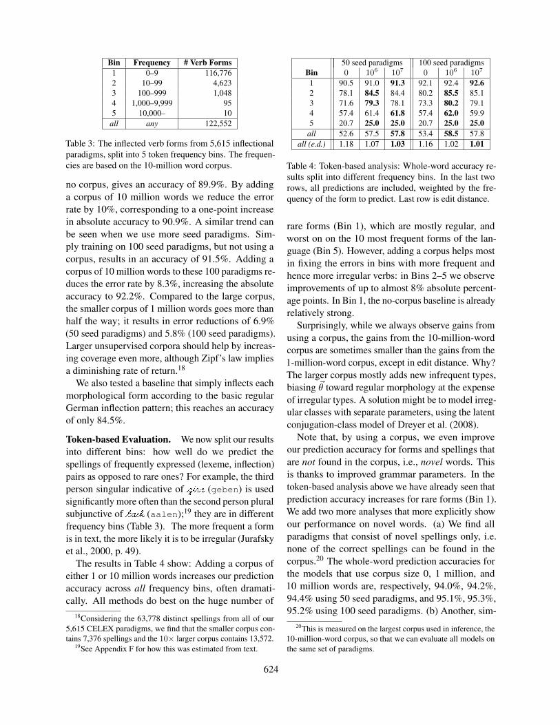
Bin Frequency # Verb Forms1 0–9 116,7762 10–99 4,6233 100–999 1,0484 1,000–9,999 955 10,000– 10

all any 122,552

Table 3: The inflected verb forms from 5,615 inflectionalparadigms, split into 5 token frequency bins. The frequen-cies are based on the 10-million word corpus.

no corpus, gives an accuracy of 89.9%. By addinga corpus of 10 million words we reduce the errorrate by 10%, corresponding to a one-point increasein absolute accuracy to 90.9%. A similar trend canbe seen when we use more seed paradigms. Sim-ply training on 100 seed paradigms, but not using acorpus, results in an accuracy of 91.5%. Adding acorpus of 10 million words to these 100 paradigms re-duces the error rate by 8.3%, increasing the absoluteaccuracy to 92.2%. Compared to the large corpus,the smaller corpus of 1 million words goes more thanhalf the way; it results in error reductions of 6.9%(50 seed paradigms) and 5.8% (100 seed paradigms).Larger unsupervised corpora should help by increas-ing coverage even more, although Zipf’s law impliesa diminishing rate of return.18

We also tested a baseline that simply inflects eachmorphological form according to the basic regularGerman inflection pattern; this reaches an accuracyof only 84.5%.

Token-based Evaluation. We now split our resultsinto different bins: how well do we predict thespellings of frequently expressed (lexeme, inflection)pairs as opposed to rare ones? For example, the thirdperson singular indicative of �g�i�v� (geben) is usedsignificantly more often than the second person pluralsubjunctive of �b$a�s�k (aalen);19 they are in differentfrequency bins (Table 3). The more frequent a formis in text, the more likely it is to be irregular (Jurafskyet al., 2000, p. 49).

The results in Table 4 show: Adding a corpus ofeither 1 or 10 million words increases our predictionaccuracy across all frequency bins, often dramati-cally. All methods do best on the huge number of

18Considering the 63,778 distinct spellings from all of our5,615 CELEX paradigms, we find that the smaller corpus con-tains 7,376 spellings and the 10× larger corpus contains 13,572.

19See Appendix F for how this was estimated from text.

50 seed paradigms 100 seed paradigmsBin 0 106 107 0 106 107

1 90.5 91.0 91.3 92.1 92.4 92.62 78.1 84.5 84.4 80.2 85.5 85.13 71.6 79.3 78.1 73.3 80.2 79.14 57.4 61.4 61.8 57.4 62.0 59.95 20.7 25.0 25.0 20.7 25.0 25.0

all 52.6 57.5 57.8 53.4 58.5 57.8all (e.d.) 1.18 1.07 1.03 1.16 1.02 1.01

Table 4: Token-based analysis: Whole-word accuracy re-sults split into different frequency bins. In the last tworows, all predictions are included, weighted by the fre-quency of the form to predict. Last row is edit distance.

rare forms (Bin 1), which are mostly regular, andworst on on the 10 most frequent forms of the lan-guage (Bin 5). However, adding a corpus helps mostin fixing the errors in bins with more frequent andhence more irregular verbs: in Bins 2–5 we observeimprovements of up to almost 8% absolute percent-age points. In Bin 1, the no-corpus baseline is alreadyrelatively strong.

Surprisingly, while we always observe gains fromusing a corpus, the gains from the 10-million-wordcorpus are sometimes smaller than the gains from the1-million-word corpus, except in edit distance. Why?The larger corpus mostly adds new infrequent types,biasing ~θ toward regular morphology at the expenseof irregular types. A solution might be to model irreg-ular classes with separate parameters, using the latentconjugation-class model of Dreyer et al. (2008).

Note that, by using a corpus, we even improveour prediction accuracy for forms and spellings thatare not found in the corpus, i.e., novel words. Thisis thanks to improved grammar parameters. In thetoken-based analysis above we have already seen thatprediction accuracy increases for rare forms (Bin 1).We add two more analyses that more explicitly showour performance on novel words. (a) We find allparadigms that consist of novel spellings only, i.e.none of the correct spellings can be found in thecorpus.20 The whole-word prediction accuracies forthe models that use corpus size 0, 1 million, and10 million words are, respectively, 94.0%, 94.2%,94.4% using 50 seed paradigms, and 95.1%, 95.3%,95.2% using 100 seed paradigms. (b) Another, sim-

20This is measured on the largest corpus used in inference, the10-million-word corpus, so that we can evaluate all models onthe same set of paradigms.

624

pler measure is the prediction accuracy on all formswhose correct spelling cannot be found in the 10-million-word corpus. Here we measure accuraciesof 91.6%, 91.8% and 91.8%, respectively, using 50seed paradigms. With 100 seed paradigms, we have93.0%, 93.4% and 93.1%. The accuracies for themodels that use a corpus are higher, but do not al-ways steadily increase as we increase the corpus size.

The token-based analysis we have conducted hereshows the strength of the corpus-based approach pre-sented in this paper. While the integrated graphi-cal models over strings (Dreyer and Eisner, 2009)can learn some basic morphology from the seedparadigms, the added corpus plays an important rolein correcting its mistakes, especially for the more fre-quent, irregular verb forms. For examples of specificerrors that the models make, see Appendix E.3.

9 Related Work

Our word-and-paradigm model seamlessly handlesnonconcatenative and concatenative morphologyalike, whereas most previous work in morphologicalknowledge discovery has modeled concatenative mor-phology only, assuming that the orthographic formof a word can be split neatly into stem and affixes—asimplifying asssumption that is convenient but oftennot entirely appropriate (Kay, 1987) (how should onesegment English stopping, hoping, or knives?).

In concatenative work, Harris (1955) finds mor-pheme boundaries and segments words accordingly,an approach that was later refined by Hafer andWeiss (1974), Déjean (1998), and many others. Theunsupervised segmentation task is tackled in theannual Morpho Challenge (Kurimo et al., 2010),where ParaMor (Monson et al., 2007) and Morfessor(Creutz and Lagus, 2005) are influential contenders.The Bayesian methods that Goldwater et al. (2006b,et seq.) use to segment between words might also beapplied to segment within words, but have no notionof paradigms. Goldsmith (2001) finds what he callssignatures—sets of affixes that are used with a givenset of stems, for example (NULL, -er, -ing, -s).Chan (2006) learns sets of morphologically relatedwords; he calls these sets paradigms but notes thatthey are not substructured entities, in contrast to theparadigms we model in this paper. His models arerestricted to concatenative and regular morphology.

Morphology discovery approaches that han-dle nonconcatenative and irregular phenomenaare more closely related to our work; they arerarer. Yarowsky and Wicentowski (2000) identifyinflection-root pairs in large corpora without supervi-sion. Using similarity as well as distributional clues,they identify even irregular pairs like take/took.Schone and Jurafsky (2001) and Baroni et al. (2002)extract whole conflation sets, like “abuse, abused,abuses, abusive, abusively, . . . ,” which mayalso be irregular. We advance this work by not onlyextracting pairs or sets of related observed words,but whole structured inflectional paradigms, in whichwe can also predict forms that have never been ob-served. On the other hand, our present model doesnot yet use contextual information; we regard this asa future opportunity (see Appendix G). Naradowskyand Goldwater (2009) add simple spelling rules tothe Bayesian model of (Goldwater et al., 2006a), en-abling it to handle some systematically nonconcate-native cases. Our finite-state transducers can handlemore diverse morphological phenomena.

10 Conclusions and Future Work

We have formulated a principled framework for si-multaneously obtaining morphological annotation,an unbounded morphological lexicon that fills com-plete structured morphological paradigms with ob-served and predicted words, and parameters of a non-concatenative generative morphology model.

We ran our sampler over a large corpus (10 millionwords), inferring everything jointly and reducing theprediction error for morphological inflections by upto 10%. We observed that adding a corpus increasesthe absolute prediction accuracy on frequently occur-ring morphological forms by up to almost 8%. Futureextensions to the model could leverage token contextfor further improvements (Appendix G).

We believe that a major goal of our field should beto build full-scale explanatory probabilistic modelsof language. While we focus here on inflectionalmorphology and evaluate the results in isolation, weregard the present work as a significant step towarda larger generative model under which Bayesianinference would reconstruct other relationships aswell (e.g., inflectional, derivational, and evolution-ary) among the words in a family of languages.

625

References

A. C. Albright. 2002. The Identification of Bases inMorphological Paradigms. Ph.D. thesis, University ofCalifornia, Los Angeles.

D. Aldous. 1985. Exchangeability and related topics.École d’été de probabilités de Saint-Flour XIII, pages1–198.

C. E. Antoniak. 1974. Mixtures of Dirichlet processeswith applications to Bayesian nonparametric problems.Annals of Statistics, 2(6):1152–1174.

R. H Baayen, R. Piepenbrock, and L. Gulikers. 1995. TheCELEX lexical database (release 2)[cd-rom]. Philadel-phia, PA: Linguistic Data Consortium, University ofPennsylvania [Distributor].

M. Baroni, J. Matiasek, and H. Trost. 2002. Unsuperviseddiscovery of morphologically related words based onorthographic and semantic similarity. In Proc. of theACL-02 Workshop on Morphological and PhonologicalLearning, pages 48–57.

M. Baroni, S. Bernardini, A. Ferraresi, and E. Zanchetta.2009. The WaCky Wide Web: A collection of verylarge linguistically processed web-crawled corpora.Language Resources and Evaluation, 43(3):209–226.

David Blackwell and James B. MacQueen. 1973. Fergu-son distributions via Pòlya urn schemes. The Annals ofStatistics, 1(2):353–355, March.

David M. Blei and Peter I. Frazier. 2010. Distance-dependent Chinese restaurant processes. In Proc. ofICML, pages 87–94.

E. Chan. 2006. Learning probabilistic paradigms formorphology in a latent class model. In Proceedings ofthe Eighth Meeting of the ACL Special Interest Groupon Computational Phonology at HLT-NAACL, pages69–78.

M. Creutz and K. Lagus. 2005. Unsupervised morphemesegmentation and morphology induction from text cor-pora using Morfessor 1.0. Computer and InformationScience, Report A, 81.

H. Déjean. 1998. Morphemes as necessary conceptfor structures discovery from untagged corpora. InProc. of the Joint Conferences on New Methods inLanguage Processing and Computational Natural Lan-guage Learning, pages 295–298.

Markus Dreyer and Jason Eisner. 2009. Graphical modelsover multiple strings. In Proc. of EMNLP, Singapore,August.

Markus Dreyer, Jason Smith, and Jason Eisner. 2008.Latent-variable modeling of string transductions withfinite-state methods. In Proc. of EMNLP, Honolulu,Hawaii, October.

Markus Dreyer. 2011. A Non-Parametric Model for theDiscovery of Inflectional Paradigms from Plain Text

Using Graphical Models over Strings. Ph.D. thesis,Johns Hopkins University.

T.S. Ferguson. 1973. A Bayesian analysis of some non-parametric problems. The annals of statistics, 1(2):209–230.

Y. Freund and R. Schapire. 1999. Large margin classifica-tion using the perceptron algorithm. Machine Learning,37(3):277–296.

J. Goldsmith. 2001. Unsupervised learning of the mor-phology of a natural language. Computational Linguis-tics, 27(2):153–198.

S. Goldwater, T. Griffiths, and M. Johnson. 2006a. In-terpolating between types and tokens by estimatingpower-law generators. In Proc. of NIPS, volume 18,pages 459–466.

S. Goldwater, T. L. Griffiths, and M. Johnson. 2006b.Contextual dependencies in unsupervised word seg-mentation. In Proc. of COLING-ACL.

P.J. Green. 1995. Reversible jump Markov chain MonteCarlo computation and Bayesian model determination.Biometrika, 82(4):711.

M. A Hafer and S. F Weiss. 1974. Word segmentationby letter successor varieties. Information Storage andRetrieval, 10:371–385.

Z. S. Harris. 1955. From phoneme to morpheme. Lan-guage, 31(2):190–222.

G.E. Hinton. 2002. Training products of experts by min-imizing contrastive divergence. Neural Computation,14(8):1771–1800.

Klara Janecki. 2000. 300 Polish Verbs. Barron’s Educa-tional Series.

E. T. Jaynes. 2003. Probability Theory: The Logic ofScience. Cambridge Univ Press. Edited by Larry Bret-thorst.

D. Jurafsky, J. H. Martin, A. Kehler, K. Vander Linden,and N. Ward. 2000. Speech and Language Processing:An Introduction to Natural Language Processing, Com-putational Linguistics, and Speech Recognition. MITPress.

M. Kay. 1987. Nonconcatenative finite-state morphology.In Proc. of EACL, pages 2–10.

M. Kurimo, S. Virpioja, V. Turunen, and K. Lagus. 2010.Morpho Challenge competition 2005–2010: Evalua-tions and results. In Proc. of ACL SIGMORPHON,pages 87–95.

P. H. Matthews. 1972. Inflectional Morphology: A Theo-retical Study Based on Aspects of Latin Verb Conjuga-tion. Cambridge University Press.

Christian Monson, Jaime Carbonell, Alon Lavie, and LoriLevin. 2007. ParaMor: Minimally supervised induc-tion of paradigm structure and morphological analysis.In Proc. of ACL SIGMORPHON, pages 117–125, June.

626

J. Naradowsky and S. Goldwater. 2009. Improving mor-phology induction by learning spelling rules. In Proc.of IJCAI, pages 1531–1536.

J. Pitman and M. Yor. 1997. The two-parameter Poisson-Dirichlet distribution derived from a stable subordinator.Annals of Probability, 25:855–900.

P. Schone and D. Jurafsky. 2001. Knowledge-free induc-tion of inflectional morphologies. In Proc. of NAACL,volume 183, pages 183–191.

J. Sethuraman. 1994. A constructive definition of Dirich-let priors. Statistica Sinica, 4(2):639–650.

N. A. Smith, D. A. Smith, and R. W. Tromble. 2005.Context-based morphological disambiguation with ran-dom fields. In Proceedings of HLT-EMNLP, pages475–482, October.

G. T. Stump. 2001. Inflectional Morphology: A Theory ofParadigm Structure. Cambridge University Press.

Y.W. Teh, M.I. Jordan, M.J. Beal, and D.M. Blei. 2006.Hierarchical Dirichlet processes. Journal of the Ameri-can Statistical Association, 101(476):1566–1581.

Yee Whye Teh. 2006. A hierarchical Bayesian languagemodel based on Pitman-Yor processes. In Proc. ofACL.

K. Toutanova and R.C. Moore. 2002. Pronunciationmodeling for improved spelling correction. In Proc. ofACL, pages 144–151.

D. Yarowsky and R. Wicentowski. 2000. Minimally su-pervised morphological analysis by multimodal align-ment. In Proc. of ACL, pages 207–216, October.

627