Discovering Higher Level Structure in Visual SLAM

980 IEEE TRANSACTIONS ON ROBOTICS, VOL. 24, NO. 5, OCTOBER 2008

Discovering Higher Level Structure in Visual SLAMAndrew P. Gee, Denis Chekhlov, Andrew Calway, and Walterio Mayol-Cuevas, Member, IEEE

Abstract—In this paper, we describe a novel method for discov-ering and incorporating higher level map structure in a real-timevisual simultaneous localization and mapping (SLAM) system. Pre-vious approaches use sparse maps populated by isolated featuressuch as 3-D points or edgelets. Although this facilitates efficientlocalization, it yields very limited scene representation and ignoresthe inherent redundancy among features resulting from physicalstructure in the scene. In this paper, higher level structure, in theform of lines and surfaces, is discovered concurrently with SLAMoperation, and then, incorporated into the map in a rigorous man-ner, attempting to maintain important cross-covariance informa-tion and allow consistent update of the feature parameters. Thisis achieved by using a bottom-up process, in which subsets of low-level features are “folded in” to a parameterization of an associatedhigher level feature, thus collapsing the state space as well as build-ing structure into the map. We demonstrate and analyze the effectsof the approach for the cases of line and plane discovery, both insimulation and within a real-time system operating with a hand-held camera in an office environment.

Index Terms—Higher level structure, Kalman filtering, machinevision, simultaneous localization and mapping (SLAM).

I. INTRODUCTION

V ISUAL simultaneous localization and mapping (SLAM)aims to use cameras to recover a representation of the en-

vironment that concurrently enables accurate pose estimation.Cameras are powerful additions to the range of sensors availablefor robotics, not only because of their small size and cost, butalso for their ability to provide a rich set of world features, suchas color, texture, motion, and structure. In mobile robotics, vi-sion has proved to be an effective companion for more traditionalsensing devices. For example, in [1], where vision is coupledwith laser ranging, the visual information is reliable enough toperform loop closure for an outdoor robot in a large sectionof an urban environment. Indeed, such is the utility of vision,that cameras have also been used as the main or only SLAMsensor, as demonstrated in the seminal work of Davison [2]–[4].

Manuscript received December 18, 2007; revised July 18, 2008. Firstpublished October 10, 2008; current version published October 31, 2008. Thispaper was recommended for publication by Associate Editor J. Leonard andEditor L. Parker upon evaluation of the reviewers, comments. The work ofA. P. Gee was supported by the Engineering and Physical Sciences ResearchCouncil (EPSRC) Equator Interdisciplinary Research Collaboration (IRC). Thework of D. Chekhlov was supported in part by the Overseas Research StudentsAwards Scheme (ORSAS), in part by the University of Bristol PostgraduateResearch Scholarship, and in part by the Leonard Wakeham Endowment.

The authors are with the Department of Computer Science, University of Bris-tol, Bristol BS8 1UB, U.K. (e-mail: [email protected]; [email protected];[email protected]; [email protected]).

This paper has supplementary downloadable material available athttp://ieeexplore.ieee.org provided by the authors. The supplementary multime-dia contains a set of four videos demonstrating the three different simulationsthat were run and the system in operation discovering planes in a real officeenvironment. Its size is 36 MB.

Color versions of one or more of the figures in this paper are available onlineat http://ieeexplore.ieee.org.

Digital Object Identifier 10.1109/TRO.2008.2004641

This enables applications for a wide range of moving platforms,where the main mapping sensor could be a single camera, suchas small domestic robots and a variety of personal devices. Forthese, visual SLAM offers the fundamental competence of be-ing spatially aware, a necessity for informed motion and taskplanning.

A. Motivation

Although there have been significant advances in visualSLAM, these have been primarily concerned with localization.In contrast, progress in developing mapping output has beensomewhat neglected. Systems have been based on maps con-sisting of sparse, isolated features, predominantly 3-D points[2], [5], [6], and also 3-D edges [7]–[9] and localized planarfacets [10]. Such minimal representations are attractive fromthe localization point of view. With judicious choice of features,image processing can be kept to a minimum, enabling real-timeoperation while maintaining good tracking performance. Re-cent work has further improved on localization to give betterrobustness by adopting different frameworks such as factoredsampling [11] by using more discriminative features [6], [12] orby incorporating relocalization methods for when normal track-ing fails [5]. While this has certainly improved the performancesignificantly, the information contained in the resulting maps isstill very limited in terms of the representation of the surround-ing environment. In this paper, we seek to address this issueby investigating mechanisms to discover, and then, incorporatehigher level map structure, such as lines and surfaces, in visualSLAM systems.

B. Related Work

The detection of higher level structure has been consideredbefore, using both visual and nonvisual sensors. In most cases,this happens after the map has been generated. For exam-ple, in [13] and [14], planes are fitted to clouds of mappedpoints determined from laser ranging. However, the discov-ered structures are not incorporated into the map as new fea-tures and so do not benefit from correlation with the rest of themap and must be refitted every time when the underlying mapchanges.

In other examples, higher level features are recovered beforethey are added into the map, such as those described in [15]–[17],where 2-D geometric primitives are fitted to sonar returns andthen used as features, and [18], [19] where 3-D planes are fittedto laser range data. The method described in [20] and [21] takesthis approach a stage further and fuses measurements from alaser range finder with vertical lines from a camera to discover2-D lines, semiplanes, and corners that can be treated togetheras single features. In [22], visual map features, such as lines,

1552-3098/$25.00 © 2008 IEEE

GEE et al.: DISCOVERING HIGHER LEVEL STRUCTURE IN VISUAL SLAM 981

walls, and points, are represented in a measurement subspacethat can vary its dimensions as more information is gatheredabout the feature.

In vision-based SLAM, maps have been enhanced by virtueof users providing annotations [23], [24], manually initializ-ing regions with geometric primitives [25], or by embeddingand recognizing known objects [26]. These systems requireuser intervention, and importantly, the structures are not ableto grow to include other features as the map continues toexpand.

C. Contribution

In contrast to the previous systems, we propose a system inwhich higher level structure is automatically introduced con-currently with SLAM operation, and importantly, the newlydiscovered structures become part of the map, coexisting seam-lessly with existing features. Moreover, this is done within asingle framework, maintaining full cross covariance betweenthe different feature types, thus enabling consistent update offeature parameters. This is achieved by augmenting the systemstate with parameters representing higher level structures in amanner similar to that described in [20] and [21]. The noveltyof the approach is that we use existing features in the map toinfer the existence of higher level structure, and then, proceedto “fold in” subsets of lower order features that already existin the system state and are consistent with the parameteriza-tion. This collapses the state space, reducing redundancy andcomputational demands, as well as giving a higher level scenedescription. The approach therefore differs both in the timingat which higher level structure is introduced and in the waythe newly discovered structure is maintained and continuallyextended.

The paper is organized as follows. We first introduce a genericSLAM framework, based around Kalman filtering, in whichhigher level structure can be incorporated into a map concur-rently with localization and mapping. This is followed by detailsof how this can be achieved for the cases of planes and lines,based on collapsing subsets of 3-D points and edgelets, respec-tively. Results of experiments in simulation and for real-timeoperation using a handheld camera within an office environ-ment are then presented, including an analysis of the differenttradeoffs within the formulation. The paper concludes with adiscussion on the directions for future work. Initial findings ofthe work were previously reported in [27].

II. VISUAL SLAM WITH HIGHER LEVEL STRUCTURE

We assume a calibrated camera moving with agile motionwhile viewing a static scene. The aim is to estimate the cam-era pose while simultaneously estimating the 3-D parameters ofstructural features, such as points, lines, or surfaces. This is doneusing a Kalman filter framework. The system state x = [v,m]T

has two partitions: one for the camera pose v = [q, t]T and onefor the structural features m = [m1 ,m2 , . . .]T . The camera ro-tation is represented by the quaternion q and t is its 3-D positionvector, both defined w.r.t. a world coordinate system. We adopt a

generalized framework for the structural partition to allow mul-tiple feature types to be mapped. Each mi denotes a parameteri-zation of a feature, for example, a position vector for a 3-D pointor the position and orientation of a planar surface. In general, weexpect the number and the types of features to vary as the cameraexplores the environment, with new features being added and oldones being removed so as to minimize computation and maintainstability.

A. Kalman Filter Formulation

The Kalman filter requires a process model and an observationmodel, encoding the assumed evolution of the state betweentime steps and the relationship between the state and the filtermeasurements, respectively [28]. Application of the filter toreal-time visual SLAM is well documented (see, e.g., [2], [29],and [6]); we, therefore, provide only a brief outline here. Weassume a constant position model for the camera motion, i.e., arandom walk, and since we are dealing with a static scene, thisgives the following process model:

xnew = f(x,w) = [∆q(wω ) ⊗ q, t + wτ ,m]T (1)

where w = [wω ,wτ ]T is a 6-D noise vector, assumed to befrom N(0,Q), ∆q(wω ) is the incremental quaternion corre-sponding to the Euler angles defined by wω , and ⊗ denotesquaternion multiplication. Note that the map parameters arepredicted to remain unchanged (we assume a static scene)and that the nonadditive noise component in the quaternionpart is necessary to give an unbiased distribution in rotationspace.

At each time step, we collect a set of measurements fromthe next frame obtained from the camera, z = [z1 , z2 , . . .]T ,where, in general, each zi will be related to the state via aseparate measurement function, i.e., zi = hi(x, e), where e isa multivariate noise vector from N(0,R). For example, whenmapping point features, the measurements are assumed to becorrupted 2-D positions of projected points and for the ithmeasurement

hi(x, e) = Π(y(v,mj )) + ei (2)

where mj is the 3-D position vector of the point associatedwith the measurement zi , y(v,mj ) denotes this position vectorin the camera coordinate system, Π denotes pinhole projec-tion for a calibrated camera, and ei is a 2-D noise vector fromN(0,Ri).

Application of the filter at each time step gives mean andcovariance estimates for the state based on the process and ob-servation models. Both of these are nonlinear, and thus, weuse the extended Kalman filter (EKF) formulation, in whichupdates are derived from linear approximations based on theJacobians of f and hi [28]. The role of the covariances withinthe filter is critical. Proper maintenance ensures that updatesare propagated among the state elements, particularly the struc-tural components, which are correlated through their mutual


dependence on the camera pose [30], [31]. This ensures con-sistency and stability of the filter. Propagation of the state co-variance through the observation model also allows for betterdata association, constraining the search for image features. Asdiscussed next, it is therefore crucial to ensure that covariancesare properly maintained for a successful filter operation.

B. Augmenting and Collapsing the State

We adopt a bottom-up process in order to incorporate higherlevel structure into a map. This works as follows. Given a mappopulated by isolated lower level features, we seek subsets thatsupport the existence of higher level structure such as linesor surfaces. With sufficient support, a parameterization of thehigher level feature is then augmented to the state with an initialestimate derived from the supporting features. Subsequently,lower level features consistent with the parameterization arelinked to that feature and transformed according to the constraintthat it imposes. This results in a collapsing of the state space,reducing redundancy. Details of how this is achieved in practiceare given in Section III.

A key aspect of the work described in this paper is that theearlier process is implemented in a rigorous manner within thefilter. For this, we draw on the procedures for transformingand expanding states [32], which also forms the basis for ini-tializing isolated features in existing systems [33]. Augmen-tation and collapsing of the state is done in such a way soas to preserve full correlation among existing and new fea-tures within the map. This ensures that parameter updatesare carried out in a consistent fashion. It can be formalizedas follows. Assume that we have an existing state estimatex = [v, m1 , . . . , mn ]T , where there are n features in the map,and that we wish to augment the state with a new (higherlevel) feature mn+1 based on an initialization measurementzo . In general, the initial estimate for the feature will be derivedfrom a combination of the measurement and the existing state,i.e., mn+1 = s(x, zo), and the augmented state covariance thenbecomes

Pnew = J[P 00 Ro

]JT (3)

J =

I

∇sv ∇sm 1 . . . ∇smn

∣∣∣∣∣∣0

∇szo

(4)

where Ro is the covariance of the measurement and ∇sv =∂s/∂v. Thus, the covariance matrix grows, as illustrated inFig. 1, and introduces the important correlations between thenew feature and the existing features in the map. For example,in the case of augmentation with a new planar feature derivedfrom a subset of point features, only the relevant Jacobians∇sm i

will be nonzero and the feature will be correlated withthe camera pose through that subset of points.

In a similar way, we can also transform an existing featureto a different representation, e.g., mnew

i = r(x), and then, the

Fig. 1. Collapsing the state space when introducing higher level structure intothe SLAM map. (Left) Map consists of point features. (Middle) Parameterizationof higher level line feature introduced into the map, expanding the state x andthe covariance Σ. (Right) State space collapses as points on the line are “foldedin” to the higher level feature.

covariance update is given by

Pnew = JPJT (5)

J =

I

∇rv . . .

0

∣∣∣∣∣∣∣∣∣

0

∇rm i

0

∣∣∣∣∣∣∣∣∣

0

. . . ∇rmn

I

(6)

where any change in the dimensions of the state is reflected inthe dimensions of the Jacobian J.

Both of the previous relationships allow us to introduce higherlevel features and collapse the state size while maintaining thecross correlations within the filter. For example, as illustratedin Fig. 1, consider a new feature mn+1 that represents a higherlevel structure and imposes a constraint on a subset of existingfeatures (a line and a set of points, respectively, in Fig. 1). Givenan initial estimate of mn+1 , we can introduce it into the systemusing (3) and the constraint can then be imposed by transform-ing the existing features into the new constrained representa-tion using (5). This collapses the state by removing redundantconstrained variables, while also maintaining the correlationsbetween the new features, the camera pose, and the remainderof the map.

III. BUILDING IN HIGHER LEVEL STRUCTURE

In practice, building higher level structure into a system maphas three distinct components: discovery—determining subsetsof isolated features that support the premise that a higher levelstructure is present; incorporation—initializing a parameteriza-tion of the higher level feature into the system state and linkingexisting features to it; and measurement—deriving measure-ments for the higher level feature in order that it and its linkedfeatures can be updated within the filter.


A. Discovery

The discovery component is essentially a segmentation taskamong existing features in a map, and we adopt a random sam-ple consensus (RANSAC) approach [34]. This involves gen-erating hypotheses from minimal sets of features randomlysampled from the subset of features having sufficient conver-gence, i.e., with variance less than some suitable thresholdσ2

RANSAC . Each hypothesis is then tested for consensus withthe rest of the set. Thus, given a minimal set of features,(m1 ,m2 , . . . ,mK ), we generate the parameters for a higherlevel feature via p = g(m1 ,m2 , . . . ,mK ), and a feature mi

is then deemed to be in consensus with the hypothesis if a dis-tance measure d(p,mi) from the hypothesized feature is lessthan some threshold dRANSAC . The choice of thresholds hereis important and essentially controls the system’s willingness tointroduce new structure into the map. We discuss this furtherand analyze the tradeoffs in Section V.

In practice, RANSAC search is not performed over the globalmap but uses a small local set of the N most recently observedfeatures. At the beginning of each search, a random feature fromthis set is chosen as a base reference and used to temporarilytransform the other features in the set and discover their relativeuncertainties using the technique described in [17]. The localcovariances of the features are used for thresholding, allowingthe discovery of local structure even when the global uncertaintyis large. We use a standard implementation of RANSAC and donot currently use the variance information within the algorithmitself, although this could be incorporated in the future, e.g.,by temporarily transforming features prior to a Mahalanobisdistance consensus test by using the hypothesized higher levelfeatures as a base frame of reference.

B. Incorporation

The hypothesis with the most consensus yields a set of inlyingfeatures from which “best-fit” parameters can be derived in orderto initialize the associated higher level feature. This marks thestart of the incorporation component.

First, a χ2 similarity test with 95% bounds is performed toensure that the proposed higher level structure is not too similarto any existing structures in the system. If the test is passed,then the state is augmented with the initial parameter estimatesand the covariance is then expanded according to (3), wheres(x, zo) denotes the derivation of the parameters from the setof inlying features. Note that since the parameters are derivedonly from the inliers, then both zo = 0 and ∇sv = 0, and weneed only to compute the Jacobians ∇sm i

. This ensures thatthe parameters are correlated with the rest of the SLAM statethrough the inlying features.

Having initialized a higher level feature, the system then seeksto link existing features to it and transform them according tothe constraint that it imposes. While we could immediately in-corporate all of the inlying features into the new structure, wechoose not to do this because the current RANSAC search doesnot fully take into account the uncertainty of the features, as dis-cussed in Section III-A. Instead, we gradually add features to the

structure, adopting the following procedure for each feature inthe map (or a local subset of features around the new structure).

1) Temporarily transform the feature using the new structureas a base reference [17] to give us the state and covariancerelative to the new structure.

2) Reject the feature if σ2max > σ2

T , where σmax is the maxi-mum standard deviation of the feature relative to the struc-ture and σT is a threshold standard deviation.

3) Reject the feature if d(p,mi) > dT , where d(p,mi) isa measure of the distance from the structure, e.g., theRANSAC consensus distance measure, and dT is a dis-tance threshold.

4) Accept the feature if its Mahalanobis distance from thestructure is less than the 95% χ2 threshold.

Features accepted for incorporation are transformed into anew representation, e.g., mnew

i = r(x), and the state covarianceupdated according to (5). This typically results in a collapsingof the state due to the constraint imposed by the higher levelfeature. For example, as described in the next section, 3-D pointfeatures linked to a planar feature are transformed into 2-Dpoints lying on the plane.

It is important to emphasize that once the higher level featureis added to the map, we are able to continue to seek for newfeatures to link to it, even if they were not initially used toestimate the higher level feature or were subsequently added tothe map after incorporation.

C. Measurement

The parameters for both the higher level feature and its linkedfeatures are updated in the usual manner within the filter. To doso, we require an observation function, linking the parameters tomeasurements obtained from the incoming image frames. Thedetails of this function will be dependent on the type of higherlevel features and specific examples are given in Section IV-A4and IV-B4 for the cases of planes and lines, respectively. Due tothe cross-covariance terms introduced between features and thehigher level structure, measurement of one will necessarily up-date the other. Therefore, it is possible to update the higher levelfeature even if we are unable to take direct measurements of it.

IV. PLANES AND LINES

In this section, we describe the specific cases of discoveringand incorporating planar and straight line structure within mapsconsisting of isolated 3-D points and edgelets, respectively. Themechanisms closely follow the steps described in Section III.We, therefore, only note the key differences and implementationdetails here.

A. 3-D Planes From Points

In the case of planes, we aim to discover the location, ex-tent, and orientation of planar structure formed by 3-D pointsbeing concurrently mapped. Once a plane has been initialized,3-D points deemed to be consistent with it are collapsed into2-D planar points, reducing the state size, and may even havetheir location on the plane fixed so that the point can be com-pletely removed from the state. However, note that since we are


interested in reducing redundancy in the system, we do not atpresent verify that the discovered planes correspond to physicalplanes in the scene (c.f. Section VII).

1) Representation: Since we want to use the plane as a co-ordinate frame for 2-D points that are “folded into” the plane,we need to parameterize the orientation of the plane aroundits normal direction as well as its origin. For convenience, weuse a nonminimal representation with a 9-D state vector sothat a new planar feature augmented to the state has the formmn+1 = [po , c1 , c2 ]T , where po is the plane origin and the ori-entation is defined by two orthonormal basis vectors, c1 and c2 ,which lie on the plane. The normal to the plane is then simply thecross product between the two basis vectors, i.e., n = c1 × c2 .A 3-D point in the map that is deemed to lie on the plane andwhose feature vector mi defines its 3-D position vector can thenbe transformed into a 2-D planar point using

mnewi = [(mi − po) · c1 , (mi − po) · c2 ]T (7)

where · denotes the dot product. Thus, for l such points on aplane, this gives a state size of 9 + 2l, compared with 3l, giving areduction in state size for l > 9. In the filter, the orthonormalityconstraint of the basis vectors is applied after every updateby displacing the mean to satisfy the constraint and updatingthe covariance to reflect this displacement (c.f. the “displOff”algorithm in [35]).

2) Discovery: The discovery of potential planar structureusing the RANSAC process is similar in approach to that usedin [36]. We require a minimum of three 3-D points to generatethe parameters for a plane hypothesis, i.e.,

po = m1 c1 = m2 − m1 c2 = m3 − m1 . (8)

Consensus for the hypothesis among other points is then de-termined using a distance measure based on a perpendicu-lar distance from the plane, i.e., for a point mi , the distanced = (mi − po) · n.

We also impose the additional criterion that the Euclidean dis-tance from the plane origin must be less than a second thresholddmax , which ensures that we only initialize planes with stronglocal support. This biases the system toward introducing planesthat are likely to match local physical structure, rather than fit-ting a geometric plane through a disperse set of points. Thisis beneficial because it is reasonable to assume that a physicalplane will contain other, currently undiscovered, coplanar pointsthat can be “folded in” to the plane in the future.

To determine the best-fit plane from the inliers resulting fromthe RANSAC process, we use a principal component approachsimilar to [19]. The origin is set to the mean and the orienta-tion parameters are determined from the principal components.Specifically, if the position vectors for l inlying points w.r.t. themean are stacked into an l × 3 matrix M, then the eigenvectorof MT M corresponding to the smallest eigenvalue gives thenormal to the plane and the other two eigenvectors give thebasis vectors within the plane. The smallest eigenvalue λmin isthe variance of the inliers in the normal direction and providesa convenient measure of the quality of the fit. It is possible forthis approach to return poorly conditioned eigenvectors if the

system is degenerate. This case can be tested by rejecting planeswith pairs of similar eigenvalues.

3) Incorporation: In order to avoid adding poor estimatesof planes to the system state, the best-fit plane generated by theRANSAC process is only initialized if l > lT and λmin < λT .The best-fit parameters are used to initialize a plane feature inthe state and the covariance is updated according to (3), wherethe Jacobian w.r.t. an inlying point feature mi is computed as

∇sm i=

[∂po

∂mi,

∂c1

∂mi,

∂c2

∂mi

]T

(9)

where ∂c1/∂mi and ∂c2/∂mj are the Jacobians of the twoeigenvectors computed using the method described in [37]. Thisensures that the plane parameters are correlated with the rest ofthe state through the inlying point features.

As an additional criterion for incorporation of the point ontothe plane, we reject the point if its distance from the plane originor any other point on the plane is greater than dmax . Again, thisis to bias the system toward accepting local planes.

4) Measurement: Here, we do not consider making a directobservation of the plane. Instead, we base the plane measure-ment on observations of the 2-D points linked to the plane. Themeasurement model for a 2-D planar point mi is very similar tothat of a standard 3-D point feature, but involves an additionalpreliminary step to convert it to a 3-D position vector p in theworld frame of reference prior to projection into the camera,i.e., from (7), we have

p = [c1 c2 ]mi + po . (10)

The predicted measurement for the planar point can then be ob-tained by passing p through the standard perspective projectionmodel in (2). The similarity between the measurement modelsmakes the implementation of planar points in the consideredEKF SLAM system very simple. The measurement Jacobianrequired by the EKF is almost the same as that for 3-D pointfeatures, except that we need to take account of the conversionin (10) when computing the Jacobian relating the observation tothe 2-D point feature, i.e.,

∂hi

∂mi=

∂hi

∂p∂p∂mi

(11)

where hi is the measurement function associated with a 3-Dpoint (2) and ∂p/∂mi is the Jacobian of the 3-D point w.r.t. the2-D planar point derived from (10). Finally, since the predictedobservation is also dependent on the position and orientation ofthe plane, a Jacobian ∂hi/∂mj relating hi to the relevant planefeature mj is also derived from (10).

5) Fixing Plane Points: If the maximum of the variances ofa 2-D planar point becomes very small relative to the plane,i.e., less than a threshold σfix , then we can consider furthercollapsing the state space by removing it completely from thestate. Instead of maintaining an estimate of its 2-D position onthe plane, we consider it as a fixed point in the plane and use itsmeasurements to update the associated planar feature directly.This leads to further reduction in the size of the state space.


B. 3-D Lines From Edgelets

Another natural option to enhance scene description beyondsparse points are edges. In this case, we consider edgelet fea-tures, which are locally straight sections of a gradient imageproposed in [7]. An edgelet is composed of a point in 3-D andits direction. By their nature, edgelets can be initialized along avariety of edge shapes by assuming that even curved edges canbe approximated by locally straight sections. In this case, we areinterested in discovering straight lines formed from collectionsof edgelets and perform a reduction in state size similar to thatof points incorporated into planes.

1) Representation: We parameterize an edgelet in 6-D, com-posed of its 3-D position ce , and unnormalized 3-D direc-tion vector de . Similarly, a 3-D line feature is defined bymn+1 = [cl ,dl ]T , where cl denotes its origin point and dl isits direction.

2) Discovery: In the RANSAC discovery component, weuse pairs of edgelets to generate line hypotheses, based on their3-D position vectors, which we found to give more reliableresults than using a single edgelet. The consensus distance mea-sure is then based on the perpendicular distance of an edgelet’s3-D position from the line and the difference in its 3-D orienta-tion. Principal components of the inlier set with most consensusthen provides an initial estimate of the line direction and themean 3-D position of the inliers is taken as the line origin.

3) Incorporation: After a line is put in the state, edgeletsdeemed to lie on the line are linked to it and transformed into1-D line points parameterized by their distance from the lineorigin. These 1-D edgelets can then be removed from the state,reducing the state size dramatically. Transforming directly fromthe 6-D edgelet representation to a fixed, 1-D representationon the line makes sense because the remaining degree of free-dom, which allows the edgelet to move along the line, is notobservable in the edgelet measurements [7], which only mea-sure perpendicular offset from the line. Also, the edgelet doesnot have a descriptor linking it to a specific point on the line,so small errors in position along the line will have no effecton the performance of the system. This is a marked contrast tothe case of points on a plane, where each point measurement isassociated through a visual descriptor to a specific feature in theimage. To transform the edgelet, we simply project it onto theline along the perpendicular direction.

4) Measurement: In contrast to the case with planes, we donot pass all of the individual observations of the line points intothe EKF. Instead, a single observation for the line is computed byprojecting each of its fixed edgelets into the image plane (with3-D orientation set to that of the line) and applying a RANSACline-fitting method to robustly fit a single line to individualedgelet measurements. The direction and position of this singleline in the image is passed into the EKF as the observationof the 3-D line. Measurement Jacobians for the EKF are thencomputed in a similar manner to (11).

This approach has two distinct benefits: 1) the number ofobservations that the EKF has to process each frame is signifi-cantly reduced and 2) the RANSAC line fitting ensures that weonly accept mutually compatible measurements of the edgelets

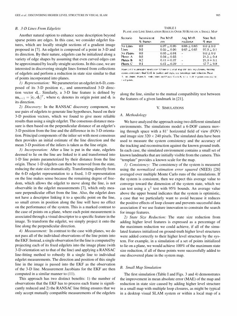
TABLE IPLANE AND LINE SIMULATION RESULTS OVER 50 RUNS ON A SMALL MAP

along the line, similar to the mutual compatibility test betweenthe features of a given landmark in [21].

V. SIMULATIONS

A. Methodology

We have analyzed the approach using two different simulatedenvironments. The simulations model a 6-DOF camera mov-ing through space with a 81◦ horizontal field of view (FOV)and image size 320× 240 pixels. The simulated data have beenused to measure the system consistency and the accuracy ofthe tracking and reconstruction against the known ground truth.In each case, the simulated environment contains a small set ofknown landmarks that are initially visible from the camera. This“template” provides a known scale for the map.

1) Consistency: The consistency of the system is measuredusing the normalized estimation error squared (NEES) [28]averaged over multiple Monte Carlo runs of the simulations. Ifthe system is consistent, then we expect this average value toconverge toward the dimension of the system state, which wecan test using a χ2 test with 95% bounds. An average valueabove the upper bound indicates that the system is optimistic,a case that we particularly want to avoid because it reducesthe positive effects of loop closure and prevents successful dataassociation if we use feature innovation to constrain the searchfor image features.

2) State Size Reduction: The state size reduction fromadding higher level features is expressed as a percentage ofthe maximum reduction we could achieve, if all of the simu-lated features initialized on ground-truth higher level structureswere added correctly to their higher level structure by the sys-tem. For example, in a simulation of a set of points initializedto lie on a plane, we would achieve 100% of the maximum statesize reduction, if all of these points were successfully added toone discovered plane in the system map.

B. Small Map Simulation

The first simulation (Table I and Figs. 3 and 4) demonstratesthe improvement in mean absolute error (MAE) of the map andreduction in state size caused by adding higher level structurein a small map with multiple loop closures, as might be typicalin a desktop visual SLAM system or within a local map of a


Fig. 2. Small map simulation results. (Top) Edgelet mapping and line dis-covery. (Bottom) Point mapping and plane discovery. A known template ofpoints/edgelets is positioned at the beginning and end of the wall to give aknown scale to the map and provide loop closure at each end. Covariance isdrawn as red ellipsoids. Ground-truth lines are drawn in pale red/cyan accordingto whether they are currently observed by the camera, and the estimated linesare superimposed on the top as thicker blue lines. The estimated plane is drawnusing a pale green bounding box around the included points. Full sequencevideos and a portable document format (PDF) version of this paper with colorimages are available in the IEEE Xplore.

submapping SLAM system. The environment contains ground-truth line or point features arranged randomly in a 4-m-longvolume and the camera translates along a sinusoidal path infront of them (Fig. 2). The positions of newly observed pointsand edgelets are initialized as 6-D inverse depth points [33] andconverted to 3-D points once their depth uncertainty becomesGaussian [38]. We assume perfect data association and Gaussianmeasurement noise of 0.5 pixel2 . Thresholds for the planes wereset at dT = 0.1 cm, σT = 1.0 cm, σRANSAC = 2σT , dmax =200 cm, and lT = 7. Thresholds for lines were set at dT =0.5 cm, 24◦, σT = 1.0 cm, 24◦, σRANSAC = σT , dmax = 120 cm,and lT = 4. The other thresholds were set in relation to thesefirst ones as dRANSAC = dT , λT = d2

T , and σfix = dT .In the line simulations, the values in Table I correspond to a

significant mean reduction in state size from 780 to 204. TheMAE in orientation and position is also improved by addinglines, as shown in Fig. 3. In particular, the relatively large co-variance on edgelet direction measurements and limited motionof the camera means that the edgelets do not quickly convergeto a good estimation on their own, so applying a line constrainthelps to overcome these limitations.

In the plane simulations, we also investigated adding clutteraround the plane by positioning 50% of the points randomlywithin ± 20 cm of the ground-truth plane (Planes B in Table I).When clutter points are prevented from being added to the planeusing ground-truth knowledge (Planes A), the results in Fig. 4show similar characteristics to the line experiments, demonstrat-ing reduction in MAE and state size, and no significant effect onconsistency of the camera or the map. When clutter points areallowed to be erroneously added to the plane (Planes B and C),this performance degrades due to the added inconsistency in themap that becomes visible at loop closure (around frame 750,Fig. 4). However, the system still achieves 0.4 cm accuracy overa 4-m map and is capable of respectable state size reductionswhen points are fixed on the plane.

Fig. 3. Small map simulation results for lines over 50 Monte Carlo runs.(Top-left) Average camera NEES remains below the upper threshold indicat-ing that the camera does not become inconsistent. (Top-right, bottom-left, andbottom-right) Evolution of MSE for the camera position, edgelet positions, andedgelet orientations respectively. Loop closure occurs around frame 750.

Fig. 4. Small map simulation results for planes over 50 Monte Carlo runs.(Top-left) Average camera NEES remains below the upper threshold indicatingthat the camera does not become inconsistent. (Top-right) Proportion of featuresthat are inconsistent increases after loop closure if outliers are erroneously addedto the plane. (Bottom-left, bottom-right) Evolution of MSE for the cameraposition and map, respectively. Loop closure occurs around frame 750.

C. Room Simulation

In the second simulation, the camera moves through a largerenvironment with 3-D points randomly arranged on and aroundthe walls of a 4-m square room (see Fig. 5). Clutter distributionand thresholds are left the same as for the previous experiments(c.f. Section V-B). The challenge in this simulation is that loopclosures occur less regularly and camera orientation error isgiven time to grow much larger.

When we allow the map to converge before adding higherlevel structure (Planes E), then consistency and MAE are com-parable to points only operation (no planes), as shown in Table IIand Fig. 6. However, we get the additional benefit of reducedstate size and improved understanding of the environment. Sim-ilar performance is achieved when we add planes to the map but


Fig. 5. Plane simulation results for Planes B. (Far-left) Initial point map-ping and plane discovery. (Center-left) Large covariance prior to loop closure.(Center-right) Covariance and map error reduction after loop closure. (Far-right)Further reduction in covariance and slight inconsistency after second loop. Pointand camera covariance shown in red and plane covariance in blue. Green linesdenote ground-truth walls and estimated planes shown as blue bounding boxesaround included points, with thickness indicating angle error. A full sequencevideo and a PDF version of this paper with color images is available in the IEEEXplore.

TABLE IIROOM SIMULATION RESULTS OVER 30 RUNS ON A ROOM MAP

Fig. 6. Consistency results over 30 Monte Carlo runs for the room simulation.(Left) Average NEES of the camera state, the horizontal lines indicate the 95%bounds on the average consistency, and the system is inconsistent if the NEESexceeds the upper bound. (Right) Proportion of points in the map with optimisticaverage consistency at each frame. Loop closure occurs around frames 2700 and5400.

do not incorporate points onto the plane (Planes D): consistencyand MAE are preserved, although in this case, the state sizeincreases since planes are added but no points are removed.

Differences in consistency only occur when the system at-tempts to incorporate points before loop closure (Planes B andC in Fig. 6). In these cases, the MAE is slightly larger but stillcomparable to the other cases. It seems as though the additionalinconsistency is caused by a combination of two factors: addingoutlier points to the plane and introducing errors when project-ing 3-D points onto the plane to enforce the planarity constraint.We intend to investigate this further in future work.

VI. REAL-WORLD EXPERIMENTS

A. Methodology

To illustrate the operation of the approach with real-worlddata, we present results obtained for plane discovery from pointswithin a real-time visual SLAM system. This operates with a

Fig. 7. Examples from a run of real-time visual SLAM with plane discoveryusing a handheld camera in an office environment. (Left) View of estimatedcamera position, 3-D mapped points, and planar features. (Right) Views throughthe camera with discovered planar features superimposed (boundaries in white)with converged 3-D points in black and 2-D planar points in white. A fullsequence video is available in the IEEE Xplore.

handheld camera and experiments were carried out in an of-fice environment containing textured planar surfaces. We use afirewire webcam with frames of size 320× 240 pixels and a 43◦

FOV. The system begins by mapping 3-D points, starting fromknown points on a calibration pattern [2]. As the camera movesaway, new points are initialized and added to the map, allowingtracking to continue as the camera explores the scene. Pointsare added using the inverse depth representation [33] and aug-mented to the state in a manner that maintains full covariancewith the rest of the map [39] (c.f. Section II-B). For measure-ments, we use the features from accelerated segment test (FAST)salient point detector [40] to identify potential features andscale-invariant feature transform (SIFT) style descriptors withscale prediction [12] for repeatable matching across frames.

B. Results

Fig. 7 shows results from an example run. On the left areexternal views of the estimated camera position and map esti-mates in terms of 3-D points and planes at different time frames.The images on the right show the view through the camera withmapped point and planar features superimposed. Note that thethree planes in the scene have been successfully discovered andincorporated into the map. The vast majority of mapped 3-Dpoints were transformed into 2-D points (except those on the cal-ibration pattern, which for fair comparison, we force to remain


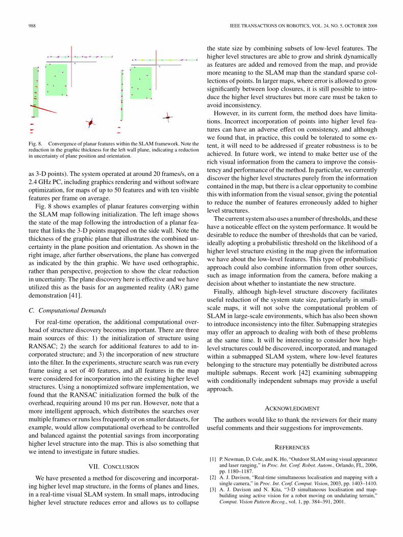
Fig. 8. Convergence of planar features within the SLAM framework. Note thereduction in the graphic thickness for the left wall plane, indicating a reductionin uncertainty of plane position and orientation.

as 3-D points). The system operated at around 20 frames/s, on a2.4 GHz PC, including graphics rendering and without softwareoptimization, for maps of up to 50 features and with ten visiblefeatures per frame on average.

Fig. 8 shows examples of planar features converging withinthe SLAM map following initialization. The left image showsthe state of the map following the introduction of a planar fea-ture that links the 3-D points mapped on the side wall. Note thethickness of the graphic plane that illustrates the combined un-certainty in the plane position and orientation. As shown in theright image, after further observations, the plane has convergedas indicated by the thin graphic. We have used orthographic,rather than perspective, projection to show the clear reductionin uncertainty. The plane discovery here is effective and we haveutilized this as the basis for an augmented reality (AR) gamedemonstration [41].

C. Computational Demands

For real-time operation, the additional computational over-head of structure discovery becomes important. There are threemain sources of this: 1) the initialization of structure usingRANSAC; 2) the search for additional features to add to in-corporated structure; and 3) the incorporation of new structureinto the filter. In the experiments, structure search was run everyframe using a set of 40 features, and all features in the mapwere considered for incorporation into the existing higher levelstructures. Using a nonoptimized software implementation, wefound that the RANSAC initialization formed the bulk of theoverhead, requiring around 10 ms per run. However, note that amore intelligent approach, which distributes the searches overmultiple frames or runs less frequently or on smaller datasets, forexample, would allow computational overhead to be controlledand balanced against the potential savings from incorporatinghigher level structure into the map. This is also something thatwe intend to investigate in future studies.

VII. CONCLUSION

We have presented a method for discovering and incorporat-ing higher level map structure, in the forms of planes and lines,in a real-time visual SLAM system. In small maps, introducinghigher level structure reduces error and allows us to collapse

the state size by combining subsets of low-level features. Thehigher level structures are able to grow and shrink dynamicallyas features are added and removed from the map, and providemore meaning to the SLAM map than the standard sparse col-lections of points. In larger maps, where error is allowed to growsignificantly between loop closures, it is still possible to intro-duce the higher level structures but more care must be taken toavoid inconsistency.

However, in its current form, the method does have limita-tions. Incorrect incorporation of points into higher level fea-tures can have an adverse effect on consistency, and althoughwe found that, in practice, this could be tolerated to some ex-tent, it will need to be addressed if greater robustness is to beachieved. In future work, we intend to make better use of therich visual information from the camera to improve the consis-tency and performance of the method. In particular, we currentlydiscover the higher level structures purely from the informationcontained in the map, but there is a clear opportunity to combinethis with information from the visual sensor, giving the potentialto reduce the number of features erroneously added to higherlevel structures.

The current system also uses a number of thresholds, and thesehave a noticeable effect on the system performance. It would bedesirable to reduce the number of thresholds that can be varied,ideally adopting a probabilistic threshold on the likelihood of ahigher level structure existing in the map given the informationwe have about the low-level features. This type of probabilisticapproach could also combine information from other sources,such as image information from the camera, before making adecision about whether to instantiate the new structure.

Finally, although high-level structure discovery facilitatesuseful reduction of the system state size, particularly in small-scale maps, it will not solve the computational problem ofSLAM in large-scale environments, which has also been shownto introduce inconsistency into the filter. Submapping strategiesmay offer an approach to dealing with both of these problemsat the same time. It will be interesting to consider how high-level structures could be discovered, incorporated, and managedwithin a submapped SLAM system, where low-level featuresbelonging to the structure may potentially be distributed acrossmultiple submaps. Recent work [42] examining submappingwith conditionally independent submaps may provide a usefulapproach.

ACKNOWLEDGMENT

The authors would like to thank the reviewers for their manyuseful comments and their suggestions for improvements.

REFERENCES

[1] P. Newman, D. Cole, and K. Ho, “Outdoor SLAM using visual appearanceand laser ranging,” in Proc. Int. Conf. Robot. Autom., Orlando, FL, 2006,pp. 1180–1187.

[2] A. J. Davison, “Real-time simultaneous localisation and mapping with asingle camera,” in Proc. Int. Conf. Comput. Vision, 2003, pp. 1403–1410.

[3] A. J. Davison and N. Kita, “3-D simultaneous localisation and map-building using active vision for a robot moving on undulating terrain,”Comput. Vision Pattern Recog., vol. 1, pp. 384–391, 2001.


[4] A. Davison and D. Murray, “Simultaneous localisation and map-buildingusing active vision,” IEEE Trans. Pattern Anal. Mach. Intell., vol. 24,no. 7, pp. 865–880, Jul. 2002.

[5] B. Williams, P. Smith, and I. Reid, “Automatic relocalisation for a single-camera simultaneous localisation and mapping system,” in Proc. Int. Conf.Robot. Autom., Rome, Italy, 2007, pp. 2784–2790.

[6] D. Chekhlov, M. Pupilli, W. Mayol, and A. Calway, “Robust real-timevisual SLAM using scale prediction and exemplar based feature descrip-tion,” in Proc. Int. Conf. Comput. Vision Pattern Recog., 2007, pp. 1–7.

[7] E. Eade and T. Drummond, “Edge landmarks in monocular SLAM,” pre-sented at the Brit. Mach. Vision Conf., 2006.

[8] P. Smith, I. Reid, and A. Davison, “Real-time monocular SLAM withstraight lines,” in Proc. Brit. Mach. Vision Conf., 2006, pp. 17–26.

[9] A. P. Gee and W. Mayol-Cuevas, “Real-time model-based SLAM usingline segments,” in Proc. Int. Symp. Visual Comput., 2006, pp. 354–363.

[10] N. Molton, I. Reid, and A. Davison, “Locally planar patch features for real-time structure from motion,” presented at the Brit. Mach. Vision Conf.,2004.

[11] E. Eade and T. Drummond, “Scalable monocular SLAM,” in Proc. Int.Conf. Comput. Vision Pattern Recog., 2006, pp. 469–476.

[12] D. Chekhlov, M. Pupilli, W. Mayol-Cuevas, and A. Calway, “Real-timeand robust monocular SLAM using predictive multi-resolution descrip-tors,” presented at the 2nd Int. Symp. Visual Comput., Nov. 2006.

[13] M. M. Nevado, J. G. Garcıa-Bermejo, and E. Zalama, “Obtaining 3-Dmodels of indoor environments with a mobile robot by estimating localsurface directions,” Robot. Auton. Syst., vol. 48, no. 2/3, pp. 131–143,Sept. 2004.

[14] D. Viejo and M. Cazorla, “3D plane-based egomotion for SLAM on semi-structured environment,” in Proc. IEEE Int. Conf. Intell. Robots Syst., SanDiego, CA, 2007, pp. 2761–2766.

[15] J. Lim and J. Leonard, “Mobile robot relocation from echolocation con-straints,” IEEE Trans. Pattern Anal. Mach. Intell., vol. 22, no. 9, pp. 1035–1041, Sept. 2000.

[16] J. J. Leonard, P. M. Newman, R. J. Rikoski, J. Neira, and J. D. Tardos,“Towards robust data association and feature modeling for concurrentmapping and localization,” in Proc. Tenth Int. Symp. Robot. Res., Lorne,Australia, Nov. 2001, pp. 9–12.

[17] J. Tardos, J. Neira, P. Newman, and J. Leonard, “Robust mapping andlocalization in indoor environments using sonar data,” Int. J. Robot. Res.,vol. 21, no. 4, pp. 311–330, 2002.

[18] J. Weingarten and R. Siegwart, “EKF-based 3D SLAM for structuredenvironment reconstruction,” in Proc. IEEE/RSJ Int. Conf. Intell. RobotsSyst., 2005, pp. 3834–3839.

[19] J. Weingarten, G. Gruener, and R. Siegwart, “Probabilistic plane fittingin 3-D and an application to robotic mapping,” in Proc. IEEE Int. Conf.Robot. Autom., New Orleans, LA, 2004, pp. 927–932.

[20] J. Castellanos and J. Tardos, Mobile Robot Localization and Map Building:A Multisensor Fusion Approach. Norwell, MA: Kluwer, 2000.

[21] J. Castellanos, J. Neira, and J. Tardos, “Multisensor fusion for simultane-ous localization and map building,” IEEE Trans. Robot. Autom., vol. 17,no. 6, pp. 908–914, Dec. 2001.

[22] J. Folkesson, P. Jensfelt, and H. Christensen, “Vision SLAM in themeasurement subspace,” in Proc. IEEE Int. Conf. Robot. Autom., 2005,Barcelona, Spain, pp. 30–35.

[23] W. Mayol, A. Davison, B. Tordoff, N. Molton, and D. Murray, “Interac-tion between hand and wearable camera in 2-D and 3-D environments,”presented at the Brit. Mach. Vision Conf., 2004.

[24] A. Davison, W. Mayol, and D. Murray, “Real-time localisation and map-ping with wearable active vision,” in Proc. IEEE ACM Int. Symp. MixedAugmented Reality, 2003, pp. 18–27.

[25] E. E. G. Reitmayr and T. Drummond, “Semi-automatic annotations inunknown environments,” in Proc. IEEE ACM Int. Symp. Mixed AugmentedReality, Nara, Japan, Nov. 2007, pp. 67–70.

[26] R. O. Castle, D. J. Gawley, G. Klein, and D. W. Murray, “Towards simul-taneous recognition, localization and mapping for hand-held and wearablecameras,” in Proc. Int. Conf. Robot. Autom., Roma, Italy, 2007, pp. 4102–4107.

[27] A. P. Gee, D. Chekhlov, W. Mayol, and A. Calway, “Discovering planesand collapsing the state space in visual SLAM,” presented at the Brit.Mach. Vision Conf., 2007.

[28] Y. Bar-Shalom, T. Kirubarajan, and X. Li, Estimation with Applicationsto Tracking and Navigation. New York: Wiley, 2002.

[29] A. Davison, I. Reid, N. Molton, and O. Stasse, “MonoSLAM: Real-timesingle camera SLAM,” IEEE Trans. Pattern Anal. Mach. Intell., vol. 29,no. 6, pp. 1052–1067, Jun. 2007.

[30] R. Smith, M. Self, and P. Cheeseman, “A stochastic map for uncertainspatial relationships,” presented at the Int. Symp. Robot. Res., 1987.

[31] H. Durrant-Whyte and T. Bailey, “Simultaneous localisation and mapping(SLAM): Part I—The essential algorithms,” IEEE Robot. Autom. Mag.,vol. 13, no. 2, pp. 99–110, Jun. 2006.

[32] T. Bailey and H. Durrant-Whyte, “Simultaneous localisation and mapping(SLAM): Part II—State of the art,” IEEE Robot. Autom. Mag., vol. 13,no. 3, pp. 108–117, Sept. 2006.

[33] J. Montiel, J. Civera, and A. Davison, “Unified inverse depth parametriza-tion for monocular SLAM,” in Proc. Robot.: Sci. Syst. Conf., 2006, pp. 16–19.

[34] M. Fischler and R. Bolles, “Random sample consensus: A paradigm formodel fitting with applications to image analysis and automated cartogra-phy,” Commun. ACM, vol. 24, no. 6, pp. 381–395, 1981.

[35] S. Julier and J. LaViola, “On Kalman filtering with nonlinear equalityconstraints,” IEEE Trans. Signal Process., vol. 55, no. 6, pp. 2774–2784,Jun. 2007.

[36] A. Bartoli, “A random sampling strategy for piecewise planar scene seg-mentation,” Comput. Vision Image Understanding, vol. 105, no. 1, pp. 42–59, 2007.

[37] T. Papadopoulo and M. Lourakis, “Estimating the jacobian of the singu-lar value decomposition: Theory and applications,” in Proc. Euro Conf.Comput. Vision, 2000, pp. 554–570.

[38] J. Civera, A. Davison, and J. Montiel, “Inverse depth to depth conversionfor monocular SLAM,” presented at the Int. Conf. Robot. Autom., 2007.

[39] T. Bailey, J. Nieto, J. Guivant, M. Stevens, and E. Nebot, “Consistency ofthe EKF-SLAM algorithm,” in Proc. Int. Conf. Intell. Robots Syst., 2006,pp. 3562–3568.

[40] E. Rosten and T. Drummond, “Machine learning for high-speed cornerdetection,” in Proc. Euro Conf. Comput. Vision, 2006, pp. 430–443.

[41] D. Chekhlov, A. P. Gee, A. Calway, and W. Mayol, “Ninja on a plane:Automatic discovery of physical planes for augmented reality using visualSLAM,” in Proc. Int. Symp. Mixed Augmented Reality (ISMAR), Nara,Japan, 2007, pp. 153–156.

[42] P. Pinies and J. Tardos, “Scalable SLAM building conditionally indepen-dent local maps,” presented at the IEE/RSJ Int. Conf. Intell. Robots Syst.,2007.

Andrew P. Gee received the M.Eng. degree in elec-trical and information sciences from Cambridge Uni-versity, Cambridge, U.K., in 2003. He is currentlyworking toward the Ph.D. degree with the Departmentof Computer Science, University of Bristol, Bristol,U.K.

His current research interests include computervision, wearable computing, and augmented reality.

Denis Chekhlov received the Masters degree in ap-plied mathematics from Belarusian State University,Minsk, Belarus, in 2004. He is currently working to-ward the Ph.D. degree in computer science with theUniversity of Bristol, Bristol, U.K.

His current research interests include computervision and robotics, in particular, robust real-timestructure-from-motion, and visual simultaneous lo-calization and mapping (SLAM).


Andrew Calway received the Ph.D. degree in com-puter science from Warwick University, Warwick,U.K., in 1989.

During 1989–1991, he was a Royal Society Visit-ing Researcher with the Computer Vision Laboratory,Linkoping University, Linkoping, Sweden. He alsoheld lecturing posts at Warwick and Cardiff Univer-sity, Cardiff, U.K. In 1998, he joined the University ofBristol, Bristol, U.K., where he is currently a SeniorLecturer with the Department of Computer Science.His current research interests include computer vi-

sion and image processing and stochastic techniques for structure from motionand 2-D and 3-D tracking, with applications in areas that include view interpo-lation and vision-guided location mapping.

Walterio Mayol-Cuevas (M’94) received the Gradu-ate degree in computer engineering from the NationalUniversity of Mexico (UNAM), Mexico City, Mexicoin 1999 and the Ph.D. degree in robotics from the Uni-versity of Oxford, St. Anne’s College, Oxford, U.K.,in 2005.

He was a founder member of the LINDA Re-search Group, UNAM. In September 2004, he wasappointed as a Lecturer (Assistant Professor) withthe Department of Computer Science, University ofBristol, Bristol, U.K., where he is currently engaged

in research on active vision and wearable computing and robotics.

Documents

Discovering Higher Level Structure in Visual SLAM