Embed Size (px)
Citation preview

Discontinuous Galerkin Finite Element Methods for
Compressible Flows
Jaap van der Vegt
Numerical Analysis and Computational Mechanics Group
Department of Applied Mathematics
University of Twente
Joint Work with
Sander Rhebergen, Onno Bokhove, Christiaan Klaij, Fedderik van der Bos
Toulouse, December 8, 2009

University of Twente - Chair Numerical Analysis and Computational Mechanics 1
Introduction
Motivation of research:
• Many important flow phenomena are modelled by nonconservative (hyperbolic)
partial differential equations, e.g. dispersed multiphase flows.
• Our aim is to develop space-time discontinuous Galerkin discretizations which are
suitable for both conservative and nonconservative partial differential equations

University of Twente - Chair Numerical Analysis and Computational Mechanics 2
Introduction
Motivation of research:
• Nonconservative hyperbolic partial differential equations contain nonconservative
products
∂xu + A(u)∂xu = 0
• The essential feature of nonconservative products is that A 6= Df , hence A is
not the Jacobian matrix of a flux function f .
• This causes problems once the solution becomes discontinuous, because the weak
solution in the classical sense of distributions then does not exist.
• This also complicates the derivation of discontinuous Galerkin discretizations since
there is no direct link with a Riemann problem.

University of Twente - Chair Numerical Analysis and Computational Mechanics 3
• Alternative: use the theory for nonconservative products from Dal Maso, LeFloch
and Murat (DLM)

University of Twente - Chair Numerical Analysis and Computational Mechanics 4
Overview of Presentation
• Overview of main results of the theory of Dal Maso, LeFloch and Murat for
nonconservative products
• Space-time DG discretization of nonconservative hyperbolic partial differential
equations
• Extension to the compressible Navier-Stokes equations
• Multigrid techniques for space-time DG discretizations
• Conclusions
University of Twente - Chair Numerical Analysis and Computational Mechanics 5
Nonconservative Products
• Consider the function u(x)
u(x) = uL + H(x − xd)(uR − uL), x, xd ∈]a, b[,
with H : R → R the Heaviside function.
• For any smooth function g : Rm → R
m the product g(u)∂xu is not defined at
x = xd since here |∂xu| → ∞.
• Introduce a smooth regularization uε of u. If the total variation of uε remains
uniformly bounded with respect to ε then Dal Maso, LeFloch and Murat (DLM)
showed that
g(u)du
dx≡ lim
ε→0g(u
ε)duε
dxgives a sense to the nonconservative product as a bounded measure.

University of Twente - Chair Numerical Analysis and Computational Mechanics 6
Effect of Path on Nonconservative Product
The limit of the regularized nonconservative product depends in general on the path
used in the regularization.
• Introduce a Lipschitz continuous path φ : [0, 1] → Rm, satisfying φ(0) = uL
and φ(1) = uR, connecting uL and uR in Rm.
• The following regularization uε for u then emerges:
uε(x) =
uL, if x ∈]a, xd − ε[,
φ(x−xd+ε
2ε ), if x ∈]xd − ε, xd + ε[, ε > 0.
uR, if x ∈]xd + ε, b[
University of Twente - Chair Numerical Analysis and Computational Mechanics 7
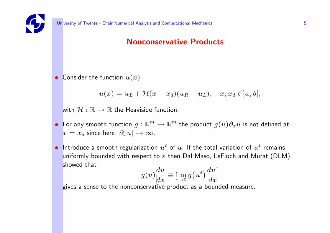
• When ε tends to zero, then:
g(uε)duε
dx Cδxd
, with C =
∫ 1
0
g(φ(τ))dφ
dτ(τ) dτ,
weakly in the sense of measures on ]a, b[, where δxdis the Dirac measure at xd.
• The limit of g(uε)∂xuε depends on the path φ.
• There is one exception, namely if an q : Rm → R exists with g = ∂uq. In this
case C = q(uR) − q(uL).

University of Twente - Chair Numerical Analysis and Computational Mechanics 8
DLM Theory
Dal Maso, LeFloch and Murat provided a general theory for nonconservative
hyperbolic pde’s.
• Introduce the Lipschitz continuous maps φ : [0, 1] × Rm × R
m → Rm which
satisfy the following properties:
(H1) φ(0; uL, uR) = uL, φ(1; uL, uR) = uR,
(H2) φ(τ ; uL, uL) = uL,
(H3)∣∣ ∂φ
∂τ (τ ; uL, uR)∣∣ ≤ K|uL − uR|, a.e. in [0, 1].

University of Twente - Chair Numerical Analysis and Computational Mechanics 9
• Theorem (DLM). Let u :]a, b[→ Rm be a function of bounded variation and
g : Rm → R
m a continuous function. Then, there exists a unique real-valued
bounded Borel measure µ on ]a, b[ with:
1. If u is continuous on a Borel set B ⊂]a, b[, then
µ(B) =
∫
B
g(u)du
dx
2. If u is discontinuous at a point xd of ]a, b[, then
µ(xd) =
∫ 1
0
g(φ(τ ; uL, uR))∂φ
∂τ(τ ; uL, uR) dτ.
By definition, this measure µ is the nonconservative product of g(u) by ∂xu and
denoted by µ =[g(u)du
dx
]φ
.

University of Twente - Chair Numerical Analysis and Computational Mechanics 10
Rankine-Hugoniot Relations
• For conservative hyperbolic system of pde’s, ∂xu + ∂xf(u) = 0 the
Rankine-Hugoniot relations across a jump with uL and uR and velocity v are
equal to
−v(uR − u
L) + f(u
R) − f(u
L) = 0.
• For a nonconservative hyperbolic pde ∂xu + A(u)∂xu = 0 the Rankine-Hugoniot
relations in the DLM theory are equal to
−v(uR − u
L) +
∫ 1
0
A(φD(s, uL, u
R))∂sφD(s; u
L, u
R)ds = 0
with φD a Lipschitz continuous path satisfying φD(0; uL, uR) = uL and
φD(1; uL, uR) = uR.
• The Rankine-Hugoniot relations are essential for the definition of the NCP flux
used in the DG discretization.

University of Twente - Chair Numerical Analysis and Computational Mechanics 11
Space-Time Discontinuous Galerkin Method
I nt n+1
tn
t0
Qn
Ω
Ω n
n+1
y
x
tK
• A time-dependent problem is considered directly in four dimensional space, with
time as the fourth dimension

University of Twente - Chair Numerical Analysis and Computational Mechanics 12
Key Features of Space-Time Discontinuous Galerkin Methods
• Simultaneous discretization in space and time: time is considered as a fourth
dimension.
• Discontinuous basis functions, both in space and time, with only a weak coupling
across element faces resulting in an extremely local, element based discretization.
• The space-time DG method is closely related to the Arbitrary Lagrangian Eulerian
(ALE) method.

University of Twente - Chair Numerical Analysis and Computational Mechanics 13
Benefits of Discontinuous Galerkin Methods
• Due to the extremely local discretization DG methods provide optimal flexibility for
I achieving higher order accuracy on unstructured meshes
I hp-mesh adaptation
I unstructured meshes containing different types of elements, such as tetrahedra,
hexahedra and prisms
I parallel computing
University of Twente - Chair Numerical Analysis and Computational Mechanics 14
Benefits of Space-Time Discontinuous Galerkin Methods
• A conservative discretization is obtained on moving and deforming meshes.
• No data interpolation or extrapolation is necessary on dynamic meshes, at free
boundaries and after mesh adaptation.

University of Twente - Chair Numerical Analysis and Computational Mechanics 15
Disadvantages of Space-(Time) Discontinuous Galerkin Methods
• Algorithms are generally rather complicated, in particular for elliptic and parabolic
partial differential equations
• On structured meshes DG methods are computationally more expensive than finite
difference and finite volume methods.

University of Twente - Chair Numerical Analysis and Computational Mechanics 16
Space-Time Domain
• Consider an open domain: E ⊂ Rd.
• The flow domain Ω(t) at time t is defined as:
Ω(t) := x ∈ E | x0 = t, t0 < t < T
• The space-time domain boundary ∂E consists of the hypersurfaces:
Ω(t0) :=x ∈ ∂E | x0 = t0,
Ω(T ) :=x ∈ ∂E | x0 = T,
Q :=x ∈ ∂E | t0 < x0 < T.
• The space-time domain is covered with a tessellation Th consisting of space-time
elements K.

University of Twente - Chair Numerical Analysis and Computational Mechanics 17
Discontinuous Finite Element Approximation
• The finite element space associated with the tessellation Th is given by:
Wh :=
W ∈ (L2(Eh))m : W |K GK ∈ (P k(K))m, ∀K ∈ Th
• The jump of f at an internal face S ∈ SnI in the direction k of a Cartesian
coordinate system is defined as:
[[f ]]k = fLnLk + fRnR
k ,
with nRk = −nL
k .
• The average of f at S ∈ SnI is defined as:
f = 12(f
L+ f
R).
University of Twente - Chair Numerical Analysis and Computational Mechanics 18
Space-Time DG Formulation of Nonconservative HyperbolicPDE’s
• Consider the nonlinear hyperbolic system of partial differential equations in
nonconservative form in multi-dimensions:
∂Ui
∂t+
∂Fik
∂xk
+ Gikr
∂Ur
∂xk
= 0, x ∈ Ω ⊂ Rq, t > 0,
with U ∈ Rm, F ∈ R
m × Rq, G ∈ R
m × Rq × R
m
• These equations model for instance bubbly flows, granular flows, shallow water
equations and many other physical systems.

University of Twente - Chair Numerical Analysis and Computational Mechanics 19
• Weak formulation for nonconservative hyperbolic system:
Find a U ∈ Vh, such that for V ∈ Vh the following relation is satisfied
∑
K∈Th
∫
KVi
(Ui,0 + Fik,k + GikrUr,k
)dK
+∑
K∈Th
( ∫
K(t−n+1)
Vi(URi − UL
i ) dK −∫
K(t+n )
Vi(URi − UL
i ) dK
)
+∑
S∈SI
∫
SVi
( ∫ 1
0
Gikr(φ(τ ; UL, U
R))
∂φr
∂τ(τ ; U
L, U
R) dτ n
Lk
)dS
−∑
S∈SI
∫
SVi[[Fik − vkUi]]k dS = 0

University of Twente - Chair Numerical Analysis and Computational Mechanics 20
Relation with Space-Time DG Formulation of ConservativeHyperbolic PDE’s
• Theorem 2. If the numerical flux V for the test function V is defined as:
V =
V at S ∈ SI,
0 at K(tn) ⊂ Ωh(tn) ∀n ≥ 0,
then the DG formulation will reduce to the conservative space-time DG formulation
when there exists a Q, such that Gikr = ∂Qik/∂Ur.

University of Twente - Chair Numerical Analysis and Computational Mechanics 21
• After the introduction of the numerical flux V we obtain the weak formulation:
∑
K∈Th
∫
K
(− Vi,0Ui − Vi,kFik + ViGikrUr,k
)dK
+∑
K∈Th
( ∫
K(t−n+1)
V Li UL
i dK −∫
K(t+n )
V Li UL
i dK
)
+∑
S∈SI
∫
S(V
Li − V
Ri )Fik − vkUin
Lk dS
+∑
S∈SB
∫
SV L
i (F Lik − vkU
Li )nL
k dS
+∑
S∈SI
∫
SVi
( ∫ 1
0
Gikr(φ(τ ; UL, U
R))
∂φr
∂τ(τ ; U
L, U
R) dτ n
Lk
)dS = 0

University of Twente - Chair Numerical Analysis and Computational Mechanics 22
Numerical Fluxes
• The fluxes at the element faces do not contain any stabilizing terms yet, both for
the conservative and nonconservative part
• At the time faces, the numerical flux is selected such that causality in time is
ensured
U =
UL at K(t−n+1)
UR at K(t+n )
.
• The space-time DG formulation is stabilized using the NCP (Non-Conservative
Product) flux
Pnci =
(Fik − vkUi + Pik
)n
Lk

University of Twente - Chair Numerical Analysis and Computational Mechanics 23
Nonconservative Product Flux
-
6
@@
@@
@@
@@
@@
@@
@@@
xL xR
x
t
SL SRSM
T
Ω1
(U = UL)
Ω4
(U = UR)
Ω2
(U = U∗
L)
Ω3
(U = U∗
R)
Wave pattern of the solution for the Riemann problem

University of Twente - Chair Numerical Analysis and Computational Mechanics 24
NCP Flux
Main steps in derivation of NCP flux:
• Consider the nonconservative hyperbolic system:
∂tU + ∂xF (U) + G(U)∂xU = 0,
• Introduce the averaged exact solution U∗LR(T ) as:
U∗LR(T ) =
1
T (SR − SL)
∫ TSR
TSL
U(x, T ) dx.
• Apply the Gauss theorem over each subdomain Ω1, · · · , Ω4 and connect each
subdomain using the generalized Rankine-Hugoniot relations.

University of Twente - Chair Numerical Analysis and Computational Mechanics 25
• The NCP-flux is then given by:
P nci (UL, UR, v, nL) =
F LiknL
k − 12
∫ 10 Gikr(φ(τ ; UL, UR))∂φr
∂τ (τ ; UL, UR) dτnLk
if SL > v,
FiknLk + 1
2
((SR − v)U∗
i + (SL − v)U∗i − SLUL
i − SRURi )
if SL < v < SR,
F RiknL
k + 12
∫ 10 Gikr(φ(τ ; UL, UR))∂φr
∂τ (τ ; UL, UR) dτnLk
if SR < v,
• Note, if G is the Jacobian of some flux function Q, then P nc(UL, UR, v, nL) is
exactly the HLL flux derived for moving grids in van der Vegt and van der Ven
(2002).
University of Twente - Chair Numerical Analysis and Computational Mechanics 26
Efficient Solution of Nonlinear Algebraic System
• The space-time DG discretization results in a large system of nonlinear algebraic
equations:
L(Un; Un−1) = 0
• This system is solved by marching to steady state using pseudo-time integration
and multigrid techniques:
∂U
∂τ= − 1
∆tL(U ; U
n−1)

University of Twente - Chair Numerical Analysis and Computational Mechanics 27
Depth averaged two-fluid model
• The dimensionless depth-averaged two fluid model of Pitman and Le, ignoring
source terms for simplicity, can be written as:
∂tU + ∂xF + G∂xU = 0,
where:
U =
h(1 − α)hαhαv
hu(1 − α)b
, F =
h(1 − α)uhαv
hαv2 + 12ε(1 − ρ)αxxgh2α
hu2 + 12εgh2
0
G(U) =
0 0 0 0 00 0 0 0 0
εραgh εραgh 0 0 ε(1 − ρ)αxxghα + εραgh
2u2α1−α − αu2 − εghα −εghα − αu2 u(α − 1) uα − 2uα
1−α (1 − α)εgh
0 0 0 0 0
.

University of Twente - Chair Numerical Analysis and Computational Mechanics 28
0 5 10 15 200
0.5
1
1.5
2
x
h(1−
α)+
b,hα
+b,
h+b,
b
h+bh(1−α)+bhα+bb
Steady-state solution for a subcritical two-phase flow (320 cells).
Total flow height h + b, flow height due to the fluid phase h(1 − α), flow height due
to solids phase hα and the topography b.

University of Twente - Chair Numerical Analysis and Computational Mechanics 29
STDGFEM
h(1 − α) + b hα + b
Ncells L2 error p Lmax error p L2 error p Lmax error p
40 0.8171 · 10−3 - 0.2308 · 10−2 - 0.1404 · 10−2 - 0.4194 · 10−2 -
80 0.2025 · 10−3 2.0 0.5584 · 10−3 2.0 0.3537 · 10−3 2.0 0.9903 · 10−3 2.1
160 0.4871 · 10−4 2.1 0.1322 · 10−3 2.1 0.8511 · 10−4 2.1 0.2306 · 10−3 2.1
320 0.9789 · 10−5 2.3 0.2651 · 10−4 2.3 0.1712 · 10−4 2.3 0.4597 · 10−4 2.3
hu(1 − α) hv(α)
Ncells L2 error p Lmax error p L2 error p Lmax error p
40 0.3672 · 10−4 - 0.1442 · 10−3 - 0.1212 · 10−4 - 0.3409 · 10−4 -
80 0.5911 · 10−5 2.6 0.3448 · 10−4 2.1 0.1791 · 10−5 2.8 0.8054 · 10−5 2.1
160 0.1049 · 10−5 2.5 0.8471 · 10−5 2.0 0.3807 · 10−6 2.2 0.2048 · 10−5 2.0
320 0.1723 · 10−6 2.6 0.2078 · 10−5 2.0 0.5115 · 10−7 2.9 0.4861 · 10−6 2.1
Error in h(1−α)+ b, hα+ b, hu(1−α) and hvα for subcritical flow over a bump.

University of Twente - Chair Numerical Analysis and Computational Mechanics 30
Two-phase dam break problem
0 0.5 10
0.5
1
1.5
2
2.5
3
3.5
x
h(1−
α),h
α,h
h(1−α) 10000hα 10000h 10000h(1−α) 128hα 128h 128
(a) Solution of h(1 − α), hα, band h.
0 0.5 1−0.5
−0.4
−0.3
−0.2
−0.1
0
0.1
0.2
0.3
x
hu(1
−α)
,hvα
hu(1−α) 10000hvα 10000hu(1−α) 128hvα 128
(b) Solution of hu(1−α) and hvα.
0 0.2 0.4 0.6 0.8 10
0.2
0.4
0.6
0.8
1
x
α
α 10000α 128
(c) Solution of α.
Two-phase dam break problem at time t = 0.175; mesh with 128 elements compared
to mesh with 10000 elements.
University of Twente - Chair Numerical Analysis and Computational Mechanics 31
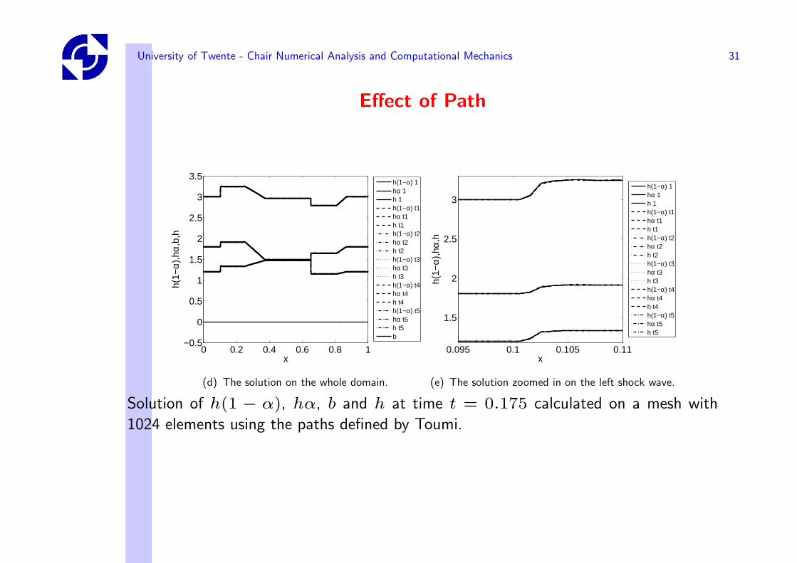
Effect of Path
0 0.2 0.4 0.6 0.8 1−0.5
0
0.5
1
1.5
2
2.5
3
3.5
x
h(1−
α),h
α,b,
h
h(1−α) 1hα 1h 1h(1−α) t1hα t1h t1h(1−α) t2hα t2h t2h(1−α) t3hα t3h t3h(1−α) t4hα t4h t4h(1−α) t5hα t5h t5b
(d) The solution on the whole domain.
0.095 0.1 0.105 0.11
1.5
2
2.5
3
x
h(1−
α),h
α,h
h(1−α) 1hα 1h 1h(1−α) t1hα t1h t1h(1−α) t2hα t2h t2h(1−α) t3hα t3h t3h(1−α) t4hα t4h t4h(1−α) t5hα t5h t5
(e) The solution zoomed in on the left shock wave.
Solution of h(1 − α), hα, b and h at time t = 0.175 calculated on a mesh with
1024 elements using the paths defined by Toumi.

University of Twente - Chair Numerical Analysis and Computational Mechanics 32
Flow Through a Contraction
x1
0
5
10
15
x2
-0.5
0
0.5
h1
Y
X
Z
h: 0.4 0.5 0.6 0.7 0.8 0.9 1 1.1 1.2 1.3 1.4 1.5
Flow depth h of water-sand mixture in a contraction
h/L = 0.01, ρf/ρs = 0.5, slope 10.

University of Twente - Chair Numerical Analysis and Computational Mechanics 33
Compressible Navier-Stokes Equations
• Compressible Navier-Stokes equations in space-time domain E :
∂Ui
∂x0
+∂F e
k(U)
∂xk
− ∂F ek(U,∇U)
∂xk
= 0
• Conservative variables U ∈ R5 and inviscid fluxes F e ∈ R
5×3
U =
ρ
ρuj
ρE
, F ek =
ρuk
ρujuk + pδjk
ρhuk
University of Twente - Chair Numerical Analysis and Computational Mechanics 34
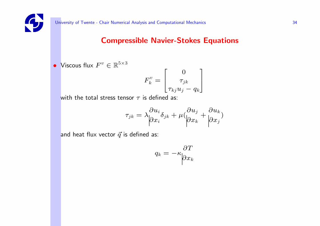
Compressible Navier-Stokes Equations
• Viscous flux F v ∈ R5×3
Fvk =
0
τjk
τkjuj − qk
with the total stress tensor τ is defined as:
τjk = λ∂ui
∂xi
δjk + µ(∂uj
∂xk
+∂uk
∂xj
)
and heat flux vector ~q is defined as:
qk = −κ∂T
∂xk

University of Twente - Chair Numerical Analysis and Computational Mechanics 35
Compressible Navier-Stokes Equations
• The viscous flux F v is homogeneous with respect to the gradient of the
conservative variables ∇U :
Fvik(U,∇U) = Aikrs(U)
∂Ur
∂xs
with the homogeneity tensor A ∈ R5×3×5×3 defined as:
Aikrs(U) :=∂F v
ik(U,∇U)
∂(∇U)
• The system is closed using the equations of state for an ideal gas.

University of Twente - Chair Numerical Analysis and Computational Mechanics 36
First Order System
• Rewrite the compressible Navier-Stokes equations as a first-order system using the
auxiliary variable Θ:
∂Ui
∂x0
+∂F e
ik(U)
∂xk
− ∂Θik(U)
∂xk
= 0,
Θik(U) − Aikrs(U)∂Ur
∂xs
= 0.
University of Twente - Chair Numerical Analysis and Computational Mechanics 37
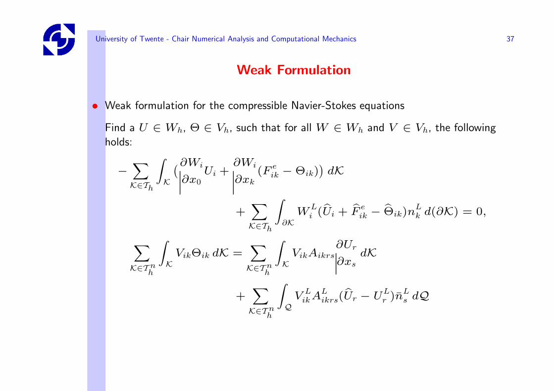
Weak Formulation
• Weak formulation for the compressible Navier-Stokes equations
Find a U ∈ Wh, Θ ∈ Vh, such that for all W ∈ Wh and V ∈ Vh, the following
holds:
−∑
K∈Th
∫
K
(∂Wi
∂x0
Ui +∂Wi
∂xk
(F eik − Θik)
)dK
+∑
K∈Th
∫
∂KW
Li (Ui + F
eik − Θik)n
Lk d(∂K) = 0,
∑
K∈T nh
∫
KVikΘik dK =
∑
K∈T nh
∫
KVikAikrs
∂Ur
∂xs
dK
+∑
K∈T nh
∫
QV L
ikALikrs(Ur − UL
r )nLs dQ

University of Twente - Chair Numerical Analysis and Computational Mechanics 38
Transformation to Arbitrary Lagrangian Eulerian form
• The space-time normal vector on a grid moving with velocity ~v is:
n =
(1, 0, 0, 0)T at K(t−n+1),
(−1, 0, 0, 0)T at K(t+n ),
(−vknk, n)T at Qn.
• The boundary integral then transforms into:
∑
K∈Th
∫
∂KW
Li (Ui + F
eik − Θik)n
Lk d(∂K)
=∑
K∈Th
( ∫
K(t−n+1)
W Li Ui dK +
∫
K(t+n )
W Li Ui dK
)
+∑
K∈Th
∫
QW
Li (F
eik − Uivk − Θik)n
Lk dQ

University of Twente - Chair Numerical Analysis and Computational Mechanics 39
Numerical Fluxes
• The numerical flux U at K(t−n+1) and K(t+n ) is defined as an upwind flux to
ensure causality in time:
U =
UL at K(t−n+1),
UR at K(t+n ),
• At the space-time faces Q we introduce the HLLC approximate Riemann solver as
numerical flux:
nk(Feik − Uivk)(U
L, UR) = HHLLCi (UL, UR, v, n)

University of Twente - Chair Numerical Analysis and Computational Mechanics 40
ALE Weak Formulation
• The ALE flux formulation of the compressible Navier-Stokes equations transforms
now into:
Find a U ∈ Wh, such that for all W ∈ Wh, the following holds:
−∑
K∈T nh
∫
K
(∂Wi
∂x0
Ui +∂Wi
∂xk
(Feik − Θik)
)dK
+∑
K∈T nh
( ∫
K(t−n+1)
WLi U
Li dK −
∫
K(t+n )
WLi U
Ri dK
)
+∑
K∈T nh
∫
QW L
i (HHLLCi (UL, UR, v, n) − Θikn
Lk ) dQ = 0.

University of Twente - Chair Numerical Analysis and Computational Mechanics 41
Lifting Operator
• Introduce the global lifting operator R ∈ R5×3, defined in a weak sense as:
Find an R ∈ Vh, such that for all V ∈ Vh:
∑
K∈T nh
∫
KVikRik dK =
∑
S∈SnI
∫
SVikAikrs[[Ur]]s dS
+∑
S∈SnB
∫
SV
LikA
Likrs(U
Lr − U
br)n
Ls dS.
• The weak formulation for the auxiliary variable is now transformed into
∑
K∈T nh
∫
KVikΘik dK =
∑
K∈T nh
∫
KVik(Aikrs
∂Ur
∂xs
− Rik) dK, ∀V ∈ Vh.

University of Twente - Chair Numerical Analysis and Computational Mechanics 42
Θ Equation
• The primal formulation can be obtained by eliminating the auxiliary variable Θ
using
Θik = Aikrs
∂Ur
∂xs
− Rik, a.e. in Enh
• Note, this is possible since ∇hWh ⊂ Vh

University of Twente - Chair Numerical Analysis and Computational Mechanics 43
ALE Weak Formulation for Primal Variables
• Recall the ALE flux formulation of the compressible Navier-Stokes equations:
Find a U ∈ Wh, such that for all W ∈ Wh, the following holds:
−∑
K∈T nh
∫
K
(∂Wi
∂x0
Ui +∂Wi
∂xk
(Feik − Θik)
)dK
+∑
K∈T nh
( ∫
K(t−n+1)
W Li UL
i dK −∫
K(t+n )
W Li UR
i dK)
+∑
K∈T nh
∫
QW L
i (HHLLCi (UL, UR, v, n) − Θikn
Lk ) dQ = 0.
University of Twente - Chair Numerical Analysis and Computational Mechanics 44
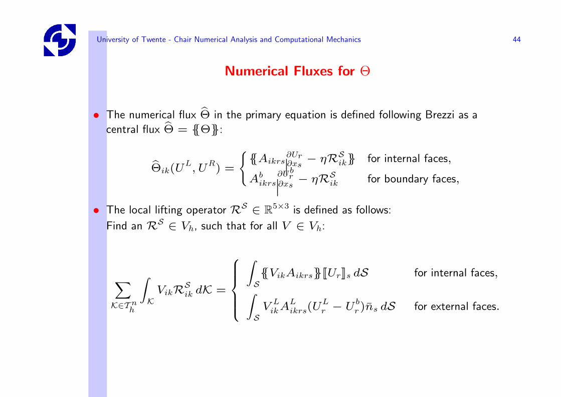
Numerical Fluxes for Θ
• The numerical flux Θ in the primary equation is defined following Brezzi as a
central flux Θ = Θ:
Θik(UL, UR) =
Aikrs
∂Ur∂xs
− ηRSik for internal faces,
Abikrs
∂Ubr
∂xs− ηRS
ik for boundary faces,
• The local lifting operator RS ∈ R5×3 is defined as follows:
Find an RS ∈ Vh, such that for all V ∈ Vh:
∑
K∈T nh
∫
KVikRS
ik dK =
∫
SVikAikrs[[Ur]]s dS for internal faces,
∫
SV L
ikALikrs(U
Lr − Ub
r)ns dS for external faces.

University of Twente - Chair Numerical Analysis and Computational Mechanics 45
Delta Wing Simulations
• Simulations of viscous flow about a delta wing with 85 sweep angle.
• Conditions
I Mach number M = 0.3
I Reynolds number Re = 40.000
I Angle of attack α = 12.5.
I Fine grid mesh 1.600.000 elements, 40.000.000 degrees of freedom
I Adapted mesh, initial mesh 208.896 elements, after four adaptations 286.416
elements

University of Twente - Chair Numerical Analysis and Computational Mechanics 46
Delta Wing Simulations
Streaklines and vorticity contours in various cross-sections

University of Twente - Chair Numerical Analysis and Computational Mechanics 47
Delta Wing Simulations
Impression of the vorticity based mesh adaptation

University of Twente - Chair Numerical Analysis and Computational Mechanics 48
Delta Wing Simulations
Large eddy simulation of turbulent flow about a delta wing

University of Twente - Chair Numerical Analysis and Computational Mechanics 49
Computational Efficiency
• Computational efficiency is the key factor limiting industrial applications of higher
order accurate discontinuous Galerkin methods in computational fluid dynamics.
• Multigrid methods are good candidates to increase computational efficiency, but
need significant improvements for higher order accurate DG discretizations.

University of Twente - Chair Numerical Analysis and Computational Mechanics 50
Objectives
• Perform a theoretical analysis of multigrid performance for advection dominated
flows, in particular for higher order accurate DG discretizations.
• Improve multigrid performance using theoretical analysis tools.
• Test multigrid performance on realistic problems.

University of Twente - Chair Numerical Analysis and Computational Mechanics 51
Main Components of h-Multigrid Algorithm
• Consider a finite sequence Nc of increasingly coarser meshes Mnh,
n ∈ 1, · · · , Nc
• Define operators to connect data on the different meshes:
I restriction operators
Rmhnh : Mnh → Mmh, 1 ≤ n < m ≤ Nc,
I prolongation operators
Pnhmh : Mmh → Mnh, 1 ≤ n < m ≤ Nc.

University of Twente - Chair Numerical Analysis and Computational Mechanics 52
• Use iterative solvers Snh to approximately solve the system of algebraic equations
on the various grid levels
Lnhvh = fnh on Mnh
• Since, the main effect of the multigrid algorithm should be the damping of high
frequency error components Snh is called a smoothing operator.
• Choose a cycling strategy between the different meshes, e.g. V- or W-cycle.

University of Twente - Chair Numerical Analysis and Computational Mechanics 53
Multigrid error transformation operator for linear problems
• In order to understand the performance of the multigrid algorithm we need to
investigate the multigrid error transformation operator.
• The multigrid error transformation operator shows how much the error in the
iterative solution of the algebraic system is reduced by one full multigrid cycle.
• We analyze three-level multigrid algorithms for 2D problems to obtain better
estimates for the convergence rate.
University of Twente - Chair Numerical Analysis and Computational Mechanics 54
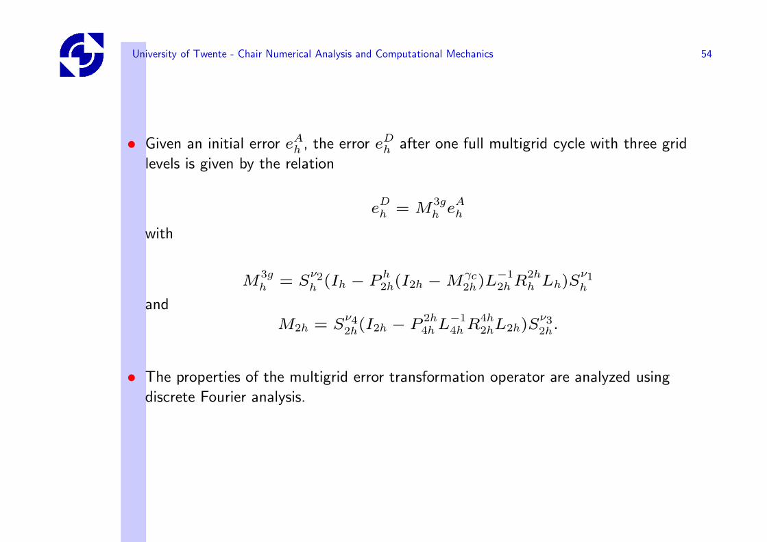
• Given an initial error eAh , the error eD
h after one full multigrid cycle with three grid
levels is given by the relation
eDh = M
3gh e
Ah
with
M3gh = S
ν2h (Ih − P
h2h(I2h − M
γc2h)L
−12h R
2hh Lh)S
ν1h
and
M2h = Sν42h(I2h − P 2h
4h L−14h R4h
2hL2h)Sν32h.
• The properties of the multigrid error transformation operator are analyzed using
discrete Fourier analysis.

University of Twente - Chair Numerical Analysis and Computational Mechanics 55
Three-grid Fourier analysis
−π −π/2 π/2 π0
0
π/2
π
−π/2
−π
θ2
θ1
π/4
−π/4
π/4
−π/4
Low, medium and high frequencies Fourier modes in three-level multigrid

University of Twente - Chair Numerical Analysis and Computational Mechanics 56
Multigrid Error Transformation Operator
• The discrete Fourier transform of the error transformation operator for a three-level
multigrid cycle M3gh (θ) ∈ C
16m×16m which is equal to
M3gh (θ) =
(S3g
h (θ))ν2
(I3g−P 3g
h (θ)U3g(θ; γc)Q3gh (θ)R3g
h (θ)L3gh (θ)
)(S3g
h (θ))ν1
∀θ ∈ Θ4h \ Ψ3g
The matrix U3g(θ; γc) is equal to
U3g(θ; γc) = I2g −(M2g
2h(2θβ))γc
.
with
M2g2h(2θβ) =
(S
2g2h(2θβ)
)ν4(
I2g−P
2g2h(2θβ)L
−14h (4θ
00)R
2g2h(2θβ)L
2g2h(2θβ)
)(S
2g2h(2θβ)
)ν3

University of Twente - Chair Numerical Analysis and Computational Mechanics 57
Asymptotic Convergence Rate
• The asymptotic convergence factor per cycle is defined as
µ = limm→∞
sup
e(0)h
6=0
‖e(m)h ‖`2(Gh)
‖e(0)h ‖`2(Gh)
1m
and can be rewritten into
µ = ρ(Mngh ).

University of Twente - Chair Numerical Analysis and Computational Mechanics 58
Optimization of multigrid performance
• The spectral radius of the error transformation operator can be used to optimize
the multigrid algorithm.
• In particular, the smoother is a good candidate for optimization since in general it
contains a number of free parameters.
• We will consider a Runge-Kutta type smoother.

University of Twente - Chair Numerical Analysis and Computational Mechanics 59
Analysis and Optimization of Runge-Kutta Smoothers for theAdvection-Diffusion Equation
• The advection-diffusion equation in the domain Ω is defined as
∂u
∂t+ a · ∇u = ∇ · (A∇u))
• The equations are discretized with a higher order accurate space-time
discontinuous Galerkin finite element method.
• The space-time discretizations are solved using a multigrid algorithm with a
Runge-Kutta type smoother.

University of Twente - Chair Numerical Analysis and Computational Mechanics 60
Pseudo-time Runge-Kutta smoothers
• Let the system of algebraic equations be denoted as
L(un, u
n−1) = 0.
• A pseudo time derivative is added to the system and integrated to steady-state in
pseudo-time
M ∂u∗
∂τ= −L(u∗, un−1),
• At steady state un = u∗.
• For the pseudo-time integration we consider 4- and 5-stage Runge-Kutta methods.

University of Twente - Chair Numerical Analysis and Computational Mechanics 61
• A four-stage Runge-Kutta scheme is given by:
(1 + β1λI)V 1 =V 0 − 1
∆x∆yα21λM−1L(V 0) + β1λV 0
(1 + β2λI)V2=V
0 − λM−1
∆x∆y
(α31L(V
0) + α32L(V
1))
+ β2λV1
(1 + β3λI)V 3 =V 0 − λM−1
∆x∆y
(α41L(V 0) + α42L(V 1) + α43L(V 2)
)+ β3λV 2
(1 + β4λI)V4=V
0 − λM−1
∆x∆y
(α51L(V
0) + α52L(V
1) + α53L(V
2) + α54L(V
3))
+β4λV3
• We require from the 4- and 5-stage Runge-Kutta schemes that they are second
order accurate
University of Twente - Chair Numerical Analysis and Computational Mechanics 62
Optimized Runge-Kutta smoothers for space-time DGFEM
• Optimization of the smoother coefficients for three-level multigrid algorithms
• Space-time DG discretization of the 2D advection-diffusion equation using
quadratic basis-functions
• For the optimization process, we fix the Reynolds numbers Rex = Rey = 100,
the flow angle γflow = π/4 and the aspect ratio AR = 1.
• For steady flows we fix CFL∆t = 100, while for unsteady flows CFL∆t = 1.

University of Twente - Chair Numerical Analysis and Computational Mechanics 63
• The optimization process has a big impact on the Runge-Kutta coefficients which
greatly differ per case.
• The Runge-Kutta coefficients are very different from commonly used schemes since
they are optimized for fast multigrid convergence and not for time accuracy.
• Finding a good balance between optimization and more generally applicable
algorithms is still an open question.
• In practice, the Runge-Kutta smoothers use local time stepping and this gives the
opportunity to apply locally the best smoother for the actual flow state.

University of Twente - Chair Numerical Analysis and Computational Mechanics 64
Optimized coefficients for dRK5 and fRK5 smoothers for 3-level multigrid (steady flow).
dRK5 p = 1 fRK5 p = 1 dRK5 p = 2 fRK5 p = 2α21 0.05768995298 0.0578331573 0.04865009589 0.04877436325α31 - -0.0002051554736 - -0.0002188348438
α32 0.1405960888 0.1403808301 0.130316854 0.1300906122α41 - 0.0003953470071 - 2.608884832e-05
α42 - -0.001195029164 - 2.444376496e-05α43 0.267958213 0.2681810517 0.2729621396 0.2734805705
α51 - 0.0001441249202 - -0.001250385487α52 - -0.0002608610327 - -0.0007838720635
α53 - -0.0003368070181 - -0.0004890887712α54 0.5 0.8473374098 0.5 4.412139367
α61 - 0.4115573097 - 0.8097217358α62 - -0.003144851878 - 0.08435089009
α63 - -0.0001096455683 - -0.01986799007α64 - 0.001555741114 - 0.01359815476
α65 1.0 0.5901414466 1.0 0.1121972094
CFLτ 0.8 0.8 0.4 0.4
ρS 0.98812 0.98914 0.98974 0.9896
ρMG 0.89151 0.81762 0.90049 0.89903
ρEXI−MG 167.06 - 124.02 -

University of Twente - Chair Numerical Analysis and Computational Mechanics 65
−10 −8 −6 −4 −2 0 2−5
−4
−3
−2
−1
0
1
2
3
4
5Stability domain of smoother
0.1
0.1
0.1
0.1
0.1
0.1
0.2
0.2
0.2
0.20.20.2
0.3
0.3
0.3
0.30.3
0.3
0.4
0.4
0.4
0.4
0.4
0.4
0.5
0.5
0.5
0.5
0.5
0.5
0.60.6
0.6
0.60.6
0.6
0.7
0.70.7
0.7
0.7
0.7
0.7
0.8
0.80.8
0.8
0.80.8
0.8
0.9
0.90.9
0.9
0.90.9
0.9
1
11
1
11
1
Re(z)
Im(z
)
(a) Stability domain dRK5.
−10 −8 −6 −4 −2 0 2−5
−4
−3
−2
−1
0
1
2
3
4
5
Re(z)
Im(z
)
Spectrum of L and stability domain of smoother
lowhigh
(b) Spectrum of Lh and stability domain dRK5.
Stability domain of dRK5 smoother and spectrum of a space-time DG discretization of
the 2D advection-diffusion equation using quadratic basis functions.

University of Twente - Chair Numerical Analysis and Computational Mechanics 66
−10 −8 −6 −4 −2 0 2−5
−4
−3
−2
−1
0
1
2
3
4
5Stability domain of smoother
0.1
0.1
0.1
0.1
0.1
0.1
0.2
0.2
0.2
0.2
0.20.2
0.3
0.3
0.3
0.3
0.30.3
0.4
0.4 0.4
0.4
0.4
0.4
0.5
0.5
0.5
0.5
0.5
0.5
0.60.6
0.6
0.60.6
0.6
0.7
0.70.7
0.7
0.70.7
0.8
0.80.8
0.8
0.80.8
0.8
0.9
0.90.9
0.9
0.90.9
0.9
1
1 1
1
11
1
Re(z)
Im(z
)
(a) Stability domain fRK5.
−10 −8 −6 −4 −2 0 2−5
−4
−3
−2
−1
0
1
2
3
4
5
Re(z)
Im(z
)
Spectrum of L and stability domain of smoother
lowhigh
(b) Spectrum of Lh and stability domain fRK5.
Stability domain of the fRK5 smoother and spectrum of a space-time DG discretization
of the 2D advection-diffusion equation using quadratic basis functions.

University of Twente - Chair Numerical Analysis and Computational Mechanics 67
−1 −0.5 0 0.5 1
−0.8
−0.6
−0.4
−0.2
0
0.2
0.4
0.6
0.8
Re
Im
Spectrum of smoother
lowhigh
(a) dRK5 smoother.
−1 −0.5 0 0.5 1
−0.8
−0.6
−0.4
−0.2
0
0.2
0.4
0.6
0.8
Re
Im
Spectrum of smoother
lowhigh
(b) fRK5 smoother.
−1 −0.5 0 0.5 1
−1
−0.8
−0.6
−0.4
−0.2
0
0.2
0.4
0.6
0.8
1
Re
Im
Spectrum of three−level operator
(c) 3-level MG with dRK5.
−1 −0.5 0 0.5 1
−1
−0.8
−0.6
−0.4
−0.2
0
0.2
0.4
0.6
0.8
1
Re
Im
Spectrum of three−level operator
(d) 3-level MG with fRK5.
Eigenvalue spectra for space-time DG discretizations of the 2D advection-diffusion
equation using quadratic basis functions.

University of Twente - Chair Numerical Analysis and Computational Mechanics 68
Testing multigrid performance
• In order to demonstrate the performance of the optimized algorithms we consider
the 2D advection-diffusion equation on a square.
• The exact steady state solution is
u(x1, x2) =1
2
(exp(a1/ν1) − exp(a1x1/ν1)
exp(a1/ν1) − 1+
exp(a2/ν2) − exp(a2x2/ν2)
exp(a2/ν2) − 1
).

University of Twente - Chair Numerical Analysis and Computational Mechanics 69
• The advection-diffusion equation is discretized using the space-time discontinuous
Galerkin discretization with quadratic basis functions.
• In the discretization we use a Shishkin mesh which is suitable for dealing with
boundary layers.
• In pseudo-time we apply a rescaling to reduce the effect of grid stretching.

University of Twente - Chair Numerical Analysis and Computational Mechanics 70
• The parameters in the tests are:
I ∆t = 100, a =√
2, νx = νy = 0.01, N1 = N2 = 32.
I Flow angle γflow = π/4.
I Depending on the stability of the smoother, we use different CFLτ and V Nτ
numbers.
I The EXV scheme was used when Rei ≤ 1 and the EXI scheme was used
otherwise.
I For the multigrid computations, ν1 = ν2 = ν3 = ν4 = 1, νC = 4 and γ = 1.
University of Twente - Chair Numerical Analysis and Computational Mechanics 71
Work units
L/L
0
500 1000 1500 2000 2500 300010-4
10-3
10-2
10-1
dRK5 coarse approx.fRK5 coarse approx.EXI/EXV coarse approx.dRK5 coarse exactfRK5 coarse exactEXI/EXV coarse exact
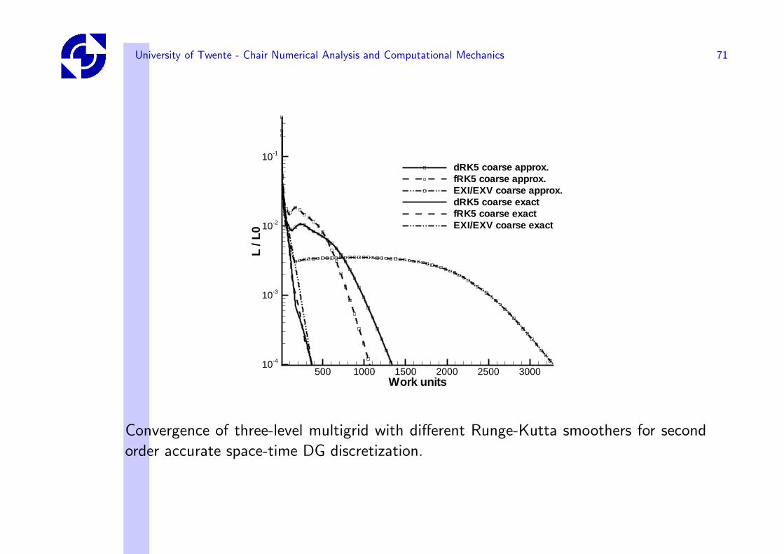
Convergence of three-level multigrid with different Runge-Kutta smoothers for second
order accurate space-time DG discretization.
University of Twente - Chair Numerical Analysis and Computational Mechanics 72
Work units
L/L
0
5000 10000 15000 2000010-4
10-3
10-2
10-1 dRK5 coarse approx.fRK5 coarse approx.EXI/EXV coarse approx.dRK5 coarse exactfRK5 coarse exactEXI/EXV coarse exact
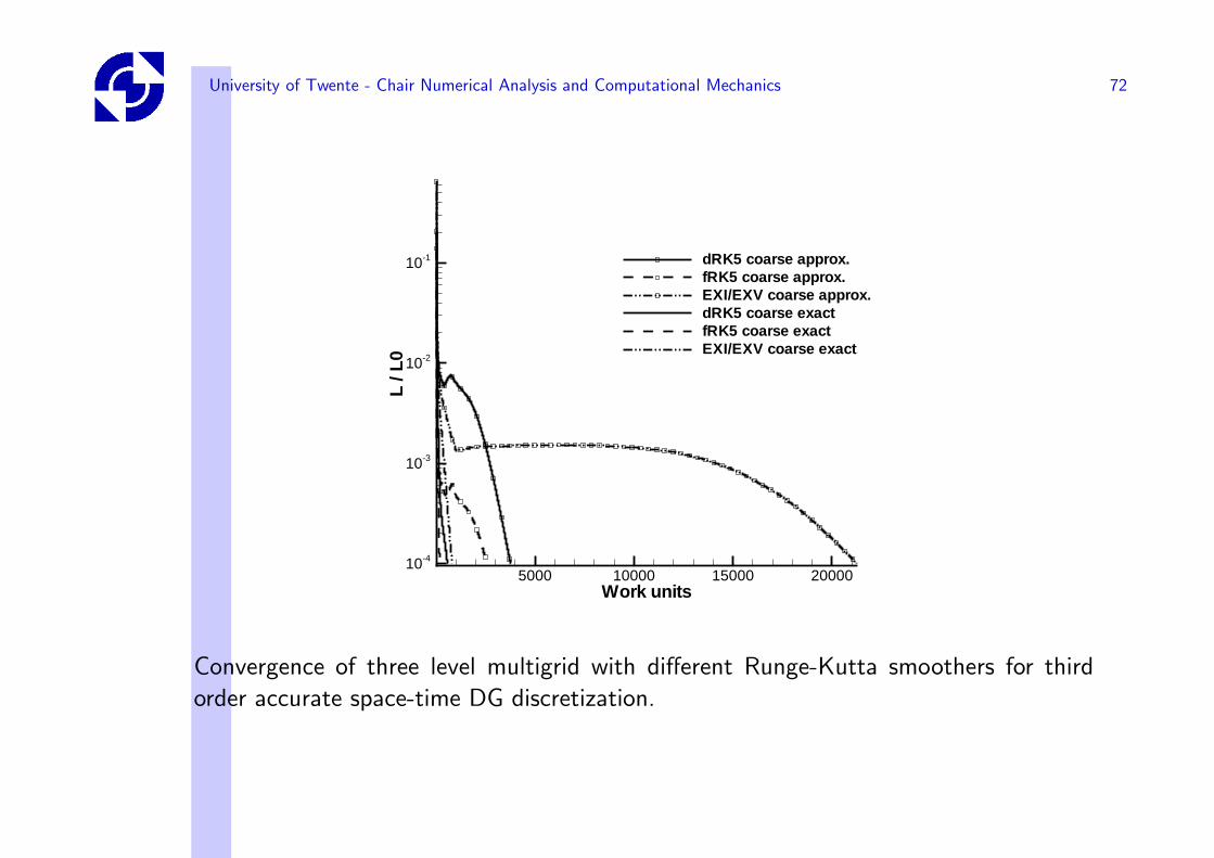
Convergence of three level multigrid with different Runge-Kutta smoothers for third
order accurate space-time DG discretization.

University of Twente - Chair Numerical Analysis and Computational Mechanics 73
We can draw the following conclusions:
• In all cases using the optimized Runge-Kutta smoothers a big improvement is
obtained over the original EXI-EXV smoother.
• For linear basis functions the number of multigrid work units to obtain 4 orders of
reduction in the residual is reduced from 3300 to 380.
• For quadratic basis functions the number of multigrid work units reduces from
22000 to 184.
• For linear basis functions the difference in convergence rate between Runge-Kutta
smoothers with only non-zero diagonal terms versus Runge-Kutta smoothers with
all coefficients non-zero is negligible.

University of Twente - Chair Numerical Analysis and Computational Mechanics 74
• For quadratic basis functions this difference is, however, significant.
• Using more Runge-Kutta coefficients enlarges the possibilities to optimize the
smoother, but the optimization process requires a significantly larger computing
time.
• In order to speed up the optimization process the coefficients of Runge-Kutta
schemes with only non-zero diagonal terms are used as initial values.

University of Twente - Chair Numerical Analysis and Computational Mechanics 75
• The effect of solving the equations on the coarsest mesh is very large.
• In particular, for nonlinear problems it is tempting to solve the algebraic system on
the coarsest mesh only approximately, but the effect is non-negligible.
• The flow angle has a small effect on the convergence rate. In general if the flow
angle is close to one of the mesh lines the convergence rate is the slowest.
• It is important not to extrapolate the results for the advection-diffusion equation
directly to the Euler and Navier-Stokes equations.

University of Twente - Chair Numerical Analysis and Computational Mechanics 76
Euler Equations
Amount of work per multigrid cycle differs single grid, p-, h-, and hp-multigrid:
work per cycle =
gpbp, SG,
(gpbp + gp−1bp−1)(νp1 + νp
2) + gp−2bp−2νpC, pMG,
gpbp((ch + ch−1)(νh
1 + νh2 ) + ch−2νh
C
), hMG,
ch(gpbp + gp−1bp−1)(νp1 + νp
2)+
gp−2bp−2((ch + ch−1)(νh1 + νh
2 ) + ch−2νhC), hpMG,
with gp and bp, respectively, the number of Gauss quadrature points and basis
functions in an element, and ch a weighting for the number of cells depending on the
grid-level h.
Coefficients: gp = 9, gp−1 = 4, gp−2 = 1, bp = 6, bp−1 = 4, bp−2 = 1, ch = 1,
ch−1 = 1/4 and ch−2 = 1/16.

University of Twente - Chair Numerical Analysis and Computational Mechanics 77
p-levels h-levels CF Lτ ρ work
1 1 1.0 0.99010 75006
3 1 1.0 0.74318 33370
3 3 1.0 0.73347 32091
1 3 1.0 0.66350 24098
1 3 0.5 0.80364 45360
Spectral radii and multigrid work units of different multigrid strategies.

University of Twente - Chair Numerical Analysis and Computational Mechanics 78
1e-10
1e-09
1e-08
1e-07
1e-06
1e-05
0.0001
0.001
0 200 400 600 800 1000 1200 1400 1600
L 2 to
tal
Work Units
SGhMG
hMG exactpMG
hpMG
Convergence history of different multigrid techniques for space-time DG discretization
for inviscid flow around a NACA0012 airfoil (MTC 1 test case, α = 2, Ma = 0.5,
448 × 64 elements).

University of Twente - Chair Numerical Analysis and Computational Mechanics 79
Conclusions
• A space-time DG discretization for nonconservative hyperbolic pde’s using the
DLM theory and the compressible Navier-Stokes has been developed.
• A new numerical flux for nonconservative hyperbolic pde’s has been developed,
which reduces to the HLLC flux for conservative pde’s.
• The effect of the choice of the path in phase space is in practice for nearly all cases
negligible.
• The algorithm has been successfully tested on a depth averaged two-phase flow
model and compressible flow simulations.

University of Twente - Chair Numerical Analysis and Computational Mechanics 80
Conclusions
• A detailed three-level multigrid analysis has been conducted for h-, p- and
hp-multigrid algorithms for the advection-diffusion and the linearized Euler
equations.
• The analysis provides the asymptotic convergence rate of the multigrid algorithms
which is used to optimize the multigrid smoothers.
• For the advection-diffusion equation the optimization results in a significant
improvement in the convergence rate in actual computations using the h-multigrid
algorithm.

University of Twente - Chair Numerical Analysis and Computational Mechanics 81
• For the Euler equations the optimized Runge-Kutta smoothers for h-, p- and
hp-multigrid show initially a significant improvement in convergence rate for
inviscid flow about a NACA 0012 airfoil, but asymptotically most algorithms have
the same convergence rate.
• Using an exact solution of the algebraic system on the coarsest mesh has a major
impact ion the convergence rate for the advection-diffusion equation, but not for
the Euler equations.