Embed Size (px)
Citation preview

Diss. ETH No. 20757
Discontinuous Galerkin FEM inComputer Graphics
A dissertation submitted to
ETH Zurich
for the Degree of
Doctor of Sciences
presented by
Peter KaufmannDipl. Informatik-Ing., ETH Zurich, Switzerlandborn February 13, 1980citizen of Meinisberg (BE), Switzerland
accepted on the recommendation of
Prof. Dr. Markus Gross, examinerProf. Dr. Olga Sorkine-Hornung, co-examinerProf. Dr. Mario Botsch, co-examiner
2013

ii

Abstract
The finite element method (FEM) is the method of choice for computing the nu-merical solution to many problems that can be formulated as partial differentialequations (PDEs) on irregular domains. Today, it is used in almost every field ofengineering and was also quickly adopted by computer graphics research where itis now heavily used in the areas of physically-based simulation and geometric mod-eling. In contrast to standard FEM, which we also refer to as continuous GalerkinFEM (CG FEM), discontinuous Galerkin FEM (DG FEM) allows its basis functionsto be discontinuous across elements. The lost coupling between elements is thenrestored by introducing penalty terms that act to reduce these discontinuities. Justlike CG FEM, DG FEM has a solid mathematical foundation and can be shown toconverge to the exact solution under certain conditions.
The reduced continuity requirements of DG FEM result in several advantages,which this thesis aims to exploit in the context of computer graphics: elementscan have arbitrary shapes; the creation of a valid element mesh as well as themodification of the mesh over time are simplified; each element is endowed withits own set of basis functions, and the quality of the approximation to the exactsolution can be chosen on a per-element basis. The work presented here appliesDG FEM in the context of physically-based simulation of deformable solids andshells, as well as image warping. The method is applied to linear as well as non-linear problems, defined through second and fourth order elliptic PDEs in twoand three spatial dimensions. In each of these applications, different aspects ofDG FEM are at the focus of attention. For the simulation of deformable solids, thearbitrary element shapes allow for topological changes without further elementremeshing. Combined with an exact integration scheme and corotated elasticity,this enables applications such as the efficient simulation of progressive cutting,dynamic mesh refinement, and a novel mesh generation approach. In the contextof shell simulations, a DG method for the Kirchhoff-Love shell equations is mergedwith the extended FEM (XFEM) to come up with a novel method for the simulationof highly detailed cutting and fracturing of shells through the use of enrichmenttextures. For image warping, DG FEM enables the generation of adaptive mesheswith higher order basis functions to make the problem of temporally consistentvideo warping more tractable.
iii

iv

Zusammenfassung
Die Methode der finiten Elemente (FEM) ist die bevorzugte Methode zur Sim-ulation vieler Probleme welche als partielle Differentialgleichungen in einem ir-regularen Gebiet formuliert werden konnen. Die Methode wird heute in praktischjedem Teilgebiet der Ingenieurwissenschaften eingesetzt und fand auch rasch imnoch relativ jungen Gebiet der Computergrafik Anwendung, dabei vorwiegendbei physikalisch basierten Simulationen sowie der geometrischen Modellierung.Im Gegensatz zur ublichen FEM, welche wir auch als continuous Galerkin FEM (CGFEM) bezeichnen, verwendet die discontinuous Galerkin FEM (DG FEM) Ansatz-funktionen, welche uber Elementgrenzen hinweg unstetig sein konnen. Diedadurch verlorene Kopplung der Elemente wird durch neu eingefuhrte Terme,welche die Diskontinuitaten penalisieren, wiederhergestellt. Ebenso wie CG FEMhat auch die DG FEM eine fundierte mathematische Basis, und es kann gezeigtwerden, dass die Methode unter gewissen Umstanden zur exakten analytischenLosung konvergiert.
Die reduzierten Stetigkeitsanforderungen der DG FEM fuhren zu einer Vielzahlvon Vorteilen, welche diese Dissertation im Kontext der Computergrafik anwendet:Elemente konnen beliebige Formen annehmen; Die Aufteilung eines Gebietes inElemente sowie die dynamische Anpassung dieser Aufteilung werden vereinfacht;Jedes Element hat seine eigenen Ansatzfunktionen und die Gute, mit welcherein Element die exakte Losung zu approximieren vermag, kann fur jedes Ele-ment einzeln gewahlt werden. Die vorliegende Arbeit verwendet DG FEM zurphysikalisch basierten Simulation von deformierbaren Festkorpern und Schalen,sowie dem Verformen von Bildern. Die Methode wird dabei auf lineare sowohlals auch nichtlineare Probleme angewendet, welche durch elliptische Differen-tialgleichungen zweiter und vierter Ordnung in zwei und drei Raumdimensio-nen definiert sind. Fur jede der gezeigten Anwendungen liegt der Schwerpunktwieder auf einem anderen Aspekte der DG FEM. Bei der Simulation von verform-baren Festkorpern wird es dank der beliebigen Elementformen moglich, topolo-gische Anderungen zu simulieren ohne dabei die zerschnittenen Elemente weiteraufteilen zu mussen. Kombiniert mit einem exakten Integrationsschema und ko-rotierter Elastizitat ermoglicht dies Anwendungen wie die effiziente Simulationder graduellen Zerschneidung von Objekten, eine dynamische Verfeinerung derElemente, sowie ein neuer Ansatz zur Erzeugung der initialen Elementaufteilung.
v

Im Kontext der Schalensimulationen wird eine DG Methode fur die Kirchhoff-LoveSchalengleichungen mit der erweiterten FEM (extended FEM) zusammengefuhrtum eine neue Methode zur Simulation von detaillierten Schnitten und Bruchenunter Verwendung von Anreicherungstexturen (enrichment textures) zu kreieren.Bei Anwendungen in der Bildverformung erlaubt DG FEM die Erzeugung vonadaptiven Elementaufteilungen mit Ansatzfunktionen hoherer Ordnung, welchedas Berechnen der zeitlich konsistenten Verformung von Videomaterial wenigeraufwandig machen.
vi

Acknowledgments
First and foremost, I want to thank my advisor Prof. Markus Gross for not givingup on convincing me that doing a Ph.D. in computer graphics is not such a badidea after all, and for introducing me to the fascinating topic of discontinuousGalerkin FEM. His broad knowledge in computer graphics and his vision of whatcould be achieved with the DG method were of great value and always driving meforward during my Ph.D.
I was very lucky to have Prof. Mario Botsch as a supervisor. He taught me the “dosand don’ts” of paper writing and I benefited tremendously from his guidance. Hisuncompromised attention to detail, his pragmatic way of approaching and solvinga problem, and the way he kept his desk completely uncluttered even during themost stressful deadlines had a lasting impression on me. I also thank Prof. EitanGrinspun for the continued collaborations, for showing us how to clearly formulatean idea and how to put that “spin” on a paper. Special thanks go to Dr. SebastianMartin, whom I had the pleasure of collaborating with on several projects. Havingsomeone like him to talk to about my projects, on a daily basis, proved to beinvaluable. Working together towards a deadline, the countless hours we spentfleshing out new ideas on the whiteboard, and the resulting “Eureka” momentswere clearly some of the most rewarding parts of my Ph.D. Big thanks to all theother people I had the chance of collaborating with and who also contributedin various ways to this thesis: Dr. Oliver Wang, Prof. Olga Sorkine-Hornung,Dr. Alex Sorkine-Hornung and Dr. Aljoscha Smolic. In addition I want to thankProf. Christoph Schwab, Prof. N. Sukumar and Prof. Max Wardetzky for theinspiring and helpful discussions.
Thanks to the past and present members of Disney Research Zurich, the ComputerGraphics Lab, the former Applied Geometry Group, and the Interactive GeometryLab for making Zurich not only one of the hotspots for graphics research, but alsoa great place to be and spend time with friends. I especially thank Dr. Gian-MarcoBaschera for his support and for contributing a lot toward the enjoyable workenvironment by being a great long term office mate.
I am also very grateful for the continuous support I received from my friendsand family, especially my parents who supported me in so many ways during mystudies.
vii

This thesis is dedicated to Elisabeth Maderthaner who taught me an awful lotabout discontinuities in real life. Lisi, I am proud of you and incredibly glad youfound your way back home again.
viii

Contents
Introduction 11.1 Overview . . . . . . . . . . . . . . . . . . . . . . . . . . . . . . . . . . 21.2 Principal Contributions . . . . . . . . . . . . . . . . . . . . . . . . . . 51.3 Thesis Outline . . . . . . . . . . . . . . . . . . . . . . . . . . . . . . . 61.4 Publications . . . . . . . . . . . . . . . . . . . . . . . . . . . . . . . . 7
Related Work 92.1 Discontinuous Galerkin FEM . . . . . . . . . . . . . . . . . . . . . . 102.2 Physically Based Simulation . . . . . . . . . . . . . . . . . . . . . . . 10
2.2.1 Simulation of Deformable Solids . . . . . . . . . . . . . . . . 112.2.2 Simulation of Thin Shells . . . . . . . . . . . . . . . . . . . . 13
2.3 Image Warping . . . . . . . . . . . . . . . . . . . . . . . . . . . . . . 14
Fundamentals 173.1 Introduction to DG FEM . . . . . . . . . . . . . . . . . . . . . . . . . 18
3.1.1 CG FEM . . . . . . . . . . . . . . . . . . . . . . . . . . . . . . 193.1.2 DG Primal Formulation . . . . . . . . . . . . . . . . . . . . . 213.1.3 DG Weak Form . . . . . . . . . . . . . . . . . . . . . . . . . . 24
3.2 DG FEM For Non-Linear Problems . . . . . . . . . . . . . . . . . . . 283.2.1 DG Derivative . . . . . . . . . . . . . . . . . . . . . . . . . . . 293.2.2 Choice of Fluxes . . . . . . . . . . . . . . . . . . . . . . . . . 313.2.3 Discretization and Lifting Operators . . . . . . . . . . . . . . 313.2.4 Stabilization . . . . . . . . . . . . . . . . . . . . . . . . . . . . 32
3.3 Non-Linear Elasticity . . . . . . . . . . . . . . . . . . . . . . . . . . . 323.3.1 Continuum Formulation . . . . . . . . . . . . . . . . . . . . . 333.3.2 Discretization and Solution . . . . . . . . . . . . . . . . . . . 36
3.4 Linear Elasticity . . . . . . . . . . . . . . . . . . . . . . . . . . . . . . 373.4.1 Continuum Formulation . . . . . . . . . . . . . . . . . . . . . 383.4.2 Discretization and Solution . . . . . . . . . . . . . . . . . . . 39
3.5 Kirchhoff-Love Shell Mechanics . . . . . . . . . . . . . . . . . . . . . 403.5.1 Shell Geometry . . . . . . . . . . . . . . . . . . . . . . . . . . 413.5.2 Shell Mechanics . . . . . . . . . . . . . . . . . . . . . . . . . . 42
3.6 Outlook . . . . . . . . . . . . . . . . . . . . . . . . . . . . . . . . . . . 44
ix

Contents
Simulation of Deformable Solids 474.1 Overview . . . . . . . . . . . . . . . . . . . . . . . . . . . . . . . . . . 484.2 Linear Elasticity using DG FEM . . . . . . . . . . . . . . . . . . . . . 49
4.2.1 DG Weak Form . . . . . . . . . . . . . . . . . . . . . . . . . . 494.2.2 Discretization and Matrix Assembly . . . . . . . . . . . . . . 51
4.3 Arbitrary Polyhedral Elements . . . . . . . . . . . . . . . . . . . . . 554.3.1 Divergence Theorem Integration . . . . . . . . . . . . . . . . 574.3.2 Integration Algorithm . . . . . . . . . . . . . . . . . . . . . . 604.3.3 Evaluation . . . . . . . . . . . . . . . . . . . . . . . . . . . . . 61
4.4 Stiffness Warping . . . . . . . . . . . . . . . . . . . . . . . . . . . . . 614.4.1 Element and Face Contributions . . . . . . . . . . . . . . . . 624.4.2 Non-Nodal Basis Functions . . . . . . . . . . . . . . . . . . . 634.4.3 Warped Assembly . . . . . . . . . . . . . . . . . . . . . . . . 63
4.5 MLS-Based Surface Embedding . . . . . . . . . . . . . . . . . . . . . 644.6 Collisions . . . . . . . . . . . . . . . . . . . . . . . . . . . . . . . . . . 664.7 Results . . . . . . . . . . . . . . . . . . . . . . . . . . . . . . . . . . . 684.8 Discussion and Outlook . . . . . . . . . . . . . . . . . . . . . . . . . 73
Enrichment Textures for Shells 755.1 Overview . . . . . . . . . . . . . . . . . . . . . . . . . . . . . . . . . . 765.2 Discontinuous Galerkin FEM Thin Shells . . . . . . . . . . . . . . . 77
5.2.1 Shell Model . . . . . . . . . . . . . . . . . . . . . . . . . . . . 775.2.2 Stiffness Matrix Assembly . . . . . . . . . . . . . . . . . . . . 795.2.3 Dynamic Simulation . . . . . . . . . . . . . . . . . . . . . . . 855.2.4 Corotational DG FEM Shells . . . . . . . . . . . . . . . . . . 85
5.3 XFEM Basics . . . . . . . . . . . . . . . . . . . . . . . . . . . . . . . . 875.4 Enrichment Textures . . . . . . . . . . . . . . . . . . . . . . . . . . . 89
5.4.1 Single Cut . . . . . . . . . . . . . . . . . . . . . . . . . . . . . 905.4.2 Multiple Cuts . . . . . . . . . . . . . . . . . . . . . . . . . . . 915.4.3 Rendering . . . . . . . . . . . . . . . . . . . . . . . . . . . . . 91
5.5 Progressive Cutting . . . . . . . . . . . . . . . . . . . . . . . . . . . . 945.5.1 Single Cut . . . . . . . . . . . . . . . . . . . . . . . . . . . . . 945.5.2 Multiple Cuts . . . . . . . . . . . . . . . . . . . . . . . . . . . 965.5.3 Multiple Elements . . . . . . . . . . . . . . . . . . . . . . . . 98
5.6 Results . . . . . . . . . . . . . . . . . . . . . . . . . . . . . . . . . . . 995.7 Discussion and Outlook . . . . . . . . . . . . . . . . . . . . . . . . . 105
Non-Linear Image Warping 1076.1 Overview . . . . . . . . . . . . . . . . . . . . . . . . . . . . . . . . . . 1086.2 FEM for Image Warping . . . . . . . . . . . . . . . . . . . . . . . . . 109
6.2.1 Continuous Warping . . . . . . . . . . . . . . . . . . . . . . . 1096.2.2 FEM Discretization . . . . . . . . . . . . . . . . . . . . . . . . 110
x

Contents
6.3 Application Specifics . . . . . . . . . . . . . . . . . . . . . . . . . . . 1126.3.1 Deformation Energy Densities . . . . . . . . . . . . . . . . . 1126.3.2 Basis Functions . . . . . . . . . . . . . . . . . . . . . . . . . . 1166.3.3 Mesh Construction . . . . . . . . . . . . . . . . . . . . . . . . 1186.3.4 Additional Constraints . . . . . . . . . . . . . . . . . . . . . . 118
6.4 Results . . . . . . . . . . . . . . . . . . . . . . . . . . . . . . . . . . . 1216.5 Discussion and Outlook . . . . . . . . . . . . . . . . . . . . . . . . . 123
Conclusion 1257.1 Discussion . . . . . . . . . . . . . . . . . . . . . . . . . . . . . . . . . 1257.2 Future Work . . . . . . . . . . . . . . . . . . . . . . . . . . . . . . . . 127
Derivations and Proofs 131A.1 Derivation of IP DG Weak Form for Linear Elasticity . . . . . . . . . 131
A.1.1 Strong Form . . . . . . . . . . . . . . . . . . . . . . . . . . . . 132A.1.2 Local Weak Form . . . . . . . . . . . . . . . . . . . . . . . . . 132A.1.3 Global Weak Form . . . . . . . . . . . . . . . . . . . . . . . . 133
A.2 Basis for Multiple Complete Cuts . . . . . . . . . . . . . . . . . . . . 135
Notation and Theorems 137B.1 Mathematical Notation . . . . . . . . . . . . . . . . . . . . . . . . . . 137B.2 Theorems . . . . . . . . . . . . . . . . . . . . . . . . . . . . . . . . . . 139
Bibliography 141
Curriculum Vitae 153
xi


C H A P T E R 1Introduction
Figure 1.1: The CG FEM (left) and DG FEM (right) solutions to a 2D elasticity problemusing three elements. One edge is constrained, while a force is applied to theopposite edge. Colors indicate the area influenced by each basis function.
Finite element methods (FEMs) have become an indispensable tool in com-puter graphics. Their primary use is for the physically-based simulation ofdeformable objects or fluids, with applications that range from computeranimation to surgery simulation. But thanks to their solid mathematical foun-dation, they find more and more applications in other areas where problemscan be formulated as partial differential equations (PDEs), such as in the fieldof geometric modeling. As with every tool, people tend to stretch the limitsof what is possible with FEM, which can lead to problems: meshes containingbadly shaped elements (slivers) cause numerical issues, or convergence may
1

Introduction
be slow in some situations (locking). However, FEMs are still an active fieldof research and new variants that address these issues are constantly beingdeveloped. This thesis focuses on one such method, namely the discontinuousGalerkin FEM (DG FEM) [Cockburn, 2003], and investigates its application toproblems in computer graphics.
DG FEM is a variant of the FEM that is characterized by its use of per-elementbasis functions. In standard continuous Galerkin FEM (CG FEM), each nodeof the element mesh is associated with a basis function, and a basis functionassumes non-zero values in all elements that share the node. In contrast, in atypical DG FEM, each basis function assumes non-zero values only withinexactly one element. As this inherently decouples the elements from eachother, a “glue” energy is introduced, defined through a so-called numericalflux, that ties the elements back together. This additional energy term can bederived mathematically and just like CG FEM, the DG formulation is accurate,in the sense that the approximation converges toward the exact solutionof the involved PDE under element refinement (while making additionalassumptions, for example on the quality of the element mesh).
In comparison to CG FEM, the use of DG FEM enables adaptive refinementof mesh elements (h-refinement) and of the basis functions’ polynomial degree(p-refinement) in a simple and efficient manner. Elements can assume arbitraryshapes and compared to CG FEM, the rules on mesh topology are less strict.The increased flexibility of DG FEM is what this thesis tries to exploit inseveral areas of computer graphics. Oftentimes additional advantages willemerge from the use of DG FEM: for the simulation of deformable solidobjects, it allows for the exact integration of basis functions over polyhedralelements. For thin shells, it simplifies the computation of additional basisfunctions that can be used to represent detailed cuts and fracture curves. Forimage warping, it enables a simple adaptive quad-tree meshing approach.
1.1 Overview
This thesis presents applications of DG FEM to three different areas of com-puter graphics: the adaptive simulation of deformable solids, simulation ofshell cutting and fracturing, and image warping with temporal consistency.
Simulation of Deformable Solids. In computer graphics, FEM simula-tions of deformable objects are mostly based on tetrahedral or hexahedralmeshes. While this allows for simple and efficient implementations, topo-logical changes of the simulation domain require complex and error-prone
2

1.1 Overview
remeshing to maintain a consistent simulation mesh. However, dynamicallyadjusting the mesh is of crucial importance in several simulation scenarios,including fracture, interactive cutting in medical applications, or adaptiverefinement of complex domains.
The use of more general polyhedral elements in FEM was shown to con-siderably simplify cutting and fracture simulations [Wicke et al., 2007;Martin et al., 2008]. However, the strict conformity constraints of standardFEM require comparatively complex shape functions for those elements. Ina slightly different context, the discontinuous element meshes of the PriMoframework enable adaptive mesh refinement for interactive shape deforma-tion [Botsch et al., 2006; 2007]. However, due to the missing physical accuracythis method is not directly useful for physically-based simulations.
This work proposes a flexible and efficient simulation technique for coro-tated linear elasticity based on the discontinuous Galerkin finite elementmethod. The presented approach conceptually generalizes the aforemen-tioned techniques, and overcomes their limitations by combining their respec-tive strengths: thanks to its convergence properties the DG FEM formulationis physically accurate and converges to the exact solution under element re-finement. Similar to PriMo, the DG approach supports arbitrary polyhedralelements and discontinuous meshes with weakly enforced continuity, therebyallowing for easy and flexible mesh restructuring.
Enrichment Textures for Shells. The simulation of thin-walled structures,i.e. shells, has a long-standing history in computer graphics. Not only do theyrequire a different mathematical treatment when compared to the simulationof solid objects, they also exhibit dramatic failure modes such as buckling,tearing, and fracturing. Simulating such phenomena requires identifyingthe location of discontinuities and predicting the response of neighboringmaterial, but even representing such discontinuities is a non-trivial task.Works in the graphics and mechanics communities have considered adaptiverefinement methods, which are well-suited for gradual variations in the scaleof relevant features, but require too many levels of refinement to sharplyresolve creases or fractures.
In an alternative point of departure, the extended finite element method(XFEM) enriches the representation with the specific basis functions requiredto capture the desired discontinuity. In doing so, XFEM introduces (unlikerefinement) only a negligible number of new unknowns, and keeps theoriginal mesh connectivity intact.
3

Introduction
In this work the XFEM is extended toward the goals of graphical simulationby representing the discontinuities in enrichment textures that allow for aresolution much higher than that of the simulation mesh. While the presentedmethod applies to arbitrary finite element methods in 2D and could evenbe extended to 3D, we focus on its application to shell simulations basedon DG FEM. There are two good reasons for using DG FEM in this context:on one hand, DG FEM is a convenient approach to shell simulation becauseit can circumvent the strict C1 continuity requirement imposed by the thinshell equations. On the other hand, the reduced continuity requirementsalso simplify the computation of the enrichment textures in our XFEM-basedmethod.
Non-Linear Image Warping. Content-aware warping has recently beenshown to be a powerful tool in a wide range of image editing applications.Warping techniques avoid difficult graphics problems such as reconstructinggeometry, global illumination, and animation, while still providing convinc-ing results. Such methods modify existing scenes by overlaying a mesh andsolving for an optimal, locally-varying deformation that minimizes someapplication-specific set of constraints.
In traditional solutions, the constraints are defined in terms of vertex finitedifferences computed on a regular grid, or by discretizing the image intoa quad mesh and computing per-quad energies from the distortion of gridedges. The error function is then minimized, generally by formulating it asa large sparse system of equations. However, these methods tightly coupleerror terms with the mesh structure, making it difficult to extend the problemformulation into new domains. Without carefully designing these errorterms, there is also no guarantee for convergence when increasing the meshresolution. Instead, this work introduces a unifying representation for a widerange of image editing tasks by using a finite element method that includesexisting finite difference metrics as a special case. A single robust mathematicalformulation of the general continuous image warping problem, combined witha finite element discretization, allows us to leverage deformation knowledgefrom mechanics and geometry communities.
Given this continuous framework, it becomes easier to validate and justifythe use of specific energy functions that drive the warping. This work dis-cusses how existing energy functions can be phrased in a continuous sense,and proposes simple novel energy functions with added benefits, such aseffective prevention of warp inversions without resorting to workarounds orincorporating inequality constraints that require quadratic programming tosolve.
4

1.2 Principal Contributions
In addition, this work presents a novel non-linear discontinuous GalerkinFEM formulation that allows working with meshes of arbitrary connectivity,with support for hanging nodes (edge nodes that do not belong to all elementsthat share the edge) that traditional FEMs cannot support. The DG FEMformulation also allows for higher order basis functions, where the order ofthe basis can be freely chosen on a per-element basis. This allows the samplingof high-resolution image information, while still performing a minimizationon a small number of elements, and it improves the smoothness of the resultswith fewer elements.
1.2 Principal Contributions
This thesis makes the following main contributions:
• A DG FEM-based simulation method for solids supporting arbi-trary polyhedral elements and topological changes. We present sev-eral extensions to the DG FEM that ultimately allow for the flexibleand efficient simulation of deformable models for computer graph-ics applications. One key problem is the integration of functionsover volumetric elements. While numerical integration is typicallyemployed here, this work presents a fast and accurate volumetricintegration technique for arbitrary polyhedral elements. To allowfor large deformations while only using a simple linear elasticitymodel, the stiffness warping approach is generalized to DG FEM. Toembed high-resolution surface meshes in coarse DG FEM meshesdespite the inherent discontinuous nature of their displacement fields,a smooth interpolation method based on moving least squares (MLS)interpolation is presented (Chapter 4).
• Harmonic Enrichment Textures. We present a unified XFEM frame-work based on harmonic enrichment functions, which allows for multi-ple, intersecting, and arbitrarily-shaped cuts per element, while beingeasy to define, compute, and use. Furthermore, a discrete representa-tion of the enrichment functions using enrichment textures simplifiesthe specification and computation of cuts and paves the way for thefuture incorporation of GPU-based techniques (Chapter 5).
• Enriched, Corotated DG FEM Thin Shells. The application of en-richment textures to thin shell simulations allows for the representa-tion of discontinuities such as creasing, tearing, cutting and fracture.Using a new corotational extension to Noels’s linear DG FEM thin
5

Introduction
shells, accurate simulations of the material’s dynamic response totime-varying discontinuities can be computed (Chapter 5).
• DG FEM Warping Framework. We propose a novel, general repre-sentation for continuous locally-varying image warping that modelsdeformation using a DG finite element method, offering advantagessuch as arbitrary mesh connectivity, a well defined, continuous prob-lem formulation, well behaved convergence properties, and supportfor higher order basis. These properties in turn allow for highly adap-tive meshes that reduce the number of degrees of freedom and makethe computation of temporally stable video retargeting solutions moretractable (Chapter 6).
• Continuous Warping Formulation. We formulate existing grid andcell-based image warping energies as continuous deformation energydensities. This allows us to relate them to material models knownfrom continuum mechanics and analyze their invariance to transla-tion, scaling and rotation. This approach further enables us to reuseprinciples from existing material models to find warp energies withcertain desirable properties such as lack of self-intersections (Chap-ter 6).
1.3 Thesis Outline
This thesis is organized as follows: Chapter 2 discusses related work in thefields of FEM, DG FEM, simulation of deformable solids, shells, and imagewarping. Chapter 3 provides an introduction to the discontinuous Galerkinfinite element method and its relation to standard (continuous) FEM for linearas well as non-linear elliptic problems. As this work focuses on the simulationof deformable objects, an introduction to non-linear elasticity theory is pro-vided, followed by its reduction to a fully linear theory. Finally, the volumetrictheory is applied to the special case of thin objects, which reproduces the stan-dard Kirchhoff-Love thin shell model. In Chapter 4, the DG FEM is applied tolinear elasticity and extended further to allow for large deformations throughcorotation. By using a novel analytic integration approach, the method canbe applied to arbitrary polyhedral elements, which allows for simple meshgeneration, adaptivity, and topological changes without re-meshing of thecut elements. Chapter 5 applies DG FEM to a corotated shell model to reducethe continuity requirements of the underlying basis functions. This, in turn,enables the development of a new method inspired by the extended finiteelement method (XFEM) which allows for the simulation of progressive cuts
6

1.4 Publications
and very detailed fracturing even when the underlying simulation mesh usesa coarse discretization. Chapter 6 applies the DG FEM in a slightly differentcontext, namely the computation of optimal image warps. A non-linear DGFEM formulation is used here, as it allows for the definition of warp energiesthat disallow element inversions and thus produce non-intersecting imagewarps. Chapter 7 concludes the thesis and discusses its main contributionsand potential future work. Additional material and proofs are given in theAppendices.
1.4 Publications
In the context of this thesis, the following publications have been accepted.
P. KAUFMANN, S. MARTIN, M. BOTSCH, and M. GROSS. Flexible Simulationof Deformable Models Using Discontinuous Galerkin FEM, Proceedings ofthe 2008 ACM SIGGRAPH/Eurographics Symposium on Computer Animation(Dublin, Ireland, July 7-9, 2008), pp. 105–115, 2008.
P. KAUFMANN, S. MARTIN, M. BOTSCH, and M. GROSS. Flexible Simulation ofDeformable Models Using Discontinuous Galerkin FEM, Journal of GraphicalModels, 2009, Special Issue of ACM SIGGRAPH / Eurographics Symposium onComputer Animation 2008, vol. 71, no. 4, pp. 153–167, 2009.
P. KAUFMANN, S. MARTIN, M. BOTSCH, E. GRINSPUN, and M. GROSS. Enrich-ment Textures for Detailed Cutting of Shells, Proceedings of ACM SIGGRAPH(New Orleans, USA, August 3-7, 2009), ACM Transactions on Graphics, vol. 28,no. 3, pp. 50:1–50:10, 2009.
P. KAUFMANN, O. WANG, A. HORNUNG, O. SORKINE, A. SMOLIC, and M.GROSS. Finite Element Image Warping, Proceedings of Eurographics (Girona,Spain, May 6-10, 2013), Computer Graphics Forum, vol. 32, no. 2, 2013
7

Introduction
8

C H A P T E R 2Related Work
Figure 2.1: Visualization of topics related to this thesis.
The finite element method has a long history in computer graphics. It hasbeen commonly used in domains such as physically based animation [Ter-zopoulos and Fleischer, 1988a], and remains the method of choice for thesimulation of deformable objects. Recent applications include geometricmodeling [Jacobson et al., 2010] and surface parameterization [Sharf et al.,2007]. One can distinguish between linear FEM where the correspondingenergy function is quadratic in the unknowns and its minimum can be foundby solving a sparse linear system, and the more general case of nonlinearFEM applicable to nonlinear minimization problems [Bonet and Wood, 1997].
9
Related Work
Next to the “standard textbook” FEM [Hughes, 2000], a number of variantsexist, including discontinuous Galerkin FEM (DG FEM) [Arnold et al., 2001],mixed FEM [Arnold, 1990], and extended FEM (XFEM) [Moes et al., 1999].
This chapter presents some of the related work on FEM relevant to computergraphics, with a focus on the physically based simulation of deformablesolids and shells. In their corresponding contexts, related work on alternativemethods such as finite difference approaches and meshless methods will bementioned as well.
2.1 Discontinuous Galerkin FEM
The discontinuous Galerkin finite element method was first proposed byReed and Hill [1973] as a method for solving neuron transport problems. Thebasic idea of DG FEM, i.e., employing discontinuous shape functions andweakly enforcing boundary constraints and inter-element continuity throughpenalty forces, is rather old [Babuska and Zlamal, 1973; Douglas and Dupont,1976]. In the last decade, however, DG FEM regained increasing attention inapplied mathematics [Arnold et al., 2001; Cockburn, 2003] and has since beensuccessfully applied to hyperbolic, parabolic, elliptic, and mixed problems.
The main strength of DG FEM is its support for irregular, non-conformingmeshes, and for shape functions of different polynomial degree, which incombination allows for flexible hp-refinement. In applied mathematics andmechanics, DG FEM has successfully been employed for linear and nonlinearelasticity [Lew et al., 2004; Ten Eyck and Lew, 2006; Wihler, 2006], whereit was shown to provide an accuracy similar to CG FEM at comparablecomputational cost. Another advantage of DG FEM is the absence of lockingeven for nearly incompressible deformable objects [Wihler, 2006]. The methodcan be customized for higher order continuity, such as weakly enforcing C1
continuity using only C0 continuous basis functions. This makes DG FEM apractical choice for the simulation of linear [Noels and Radovitzky, 2008] andnon-linear [Noels, 2009] shells. DG FEM can also be combined with othermethods. For example, a combination of DG FEM and extended FEM (XFEM)was studied by Gracie et al. [2008].
2.2 Physically Based Simulation
In computer graphics, Terzopoulos et al. [1987] pioneered the use physically-based methods for graphics application, and they have since been successfully
10

2.2 Physically Based Simulation
employed for the simulation of deformable solids [Muller et al., 2002], thinshells [Grinspun et al., 2003], cloth [Baraff and Witkin, 1998], and fluids [Stam,1999]. For the related work presented here, our focus is on the simulationof deformable solid objects and shells. In both cases, we also look at exist-ing approaches for the simulation of fracture, cutting, and mesh adaptivity.What these effects have in common is that they require changes to the under-lying discretization, which in turn is closely dependent on the underlyingsimulation method.
2.2.1 Simulation of Deformable Solids
Most real-world materials exhibit a highly non-linear deformation behaviorwhen put under stress, and the need to handle large rotational deformationsof objects leads to non-linear deformation models. However, since physicalaccuracy is not the primary goal in most graphics applications, one can oftenresort to the physically plausible, robust, and efficient corotated linear elastic-ity [Muller and Gross, 2004; Hauth and Strasser, 2004] instead of running afull non-linear simulation. To alleviate some of the problems associated withFEM simulations, such as locking for nearly incompressible materials, meth-ods have been introduced that automatically reduce the physical accuracy ofthe simulation when these problems occur [Irving et al., 2007]. For a moredetailed survey of this topic the reader may consult Nealen et al. [2006].
Cutting & Fracture of Solids. The simulation of cutting and fracture of de-formable objects dates back to the pioneering work of Terzopoulos et al. [1987;1988b], and was brought to the forefront by O’Brien and Hodgins [1999]in their work on brittle (and ductile [2002]) fracture of volumetric elastica.As an alternative to simulation, some have considered purely proceduralapproaches [Desbenoit et al., 2005]. However, we focus our discussion tophysically simulated material response in the presence of cuts and fracture.
When combined with FEM, the topological changes induced by cutting posetwo distinct challenges: first, to adapt basis functions, boundary conditions,and to update the stiffness matrix; second, to restructure the underlying meshconnectivity so as to represent the newly-created surfaces at a high resolution.Most research has focused on solid objects, where the problem of updatingmesh connectivity is particularly challenging.
Apart from simply removing the primitives of the underlying elementmesh touched by the cutting plane [Forest et al., 2002], fracturing of de-formable solids can efficiently be performed by restricting cuts to exist-
11

Related Work
ing element boundaries or predefined positions [Muller and Gross, 2004;Terzopoulos and Fleischer, 1988b]. However, these approaches are typ-ically not accurate enough for more sophisticated simulations. Splittingindividual elements allows for precise fracturing and cutting, but in turnrequires element decompositions [Bielser et al., 1999; Bielser and Gross, 2000;Bielser et al., 2003] and/or general remeshing [O’Brien and Hodgins, 1999;O’Brien et al., 2002; Steinemann et al., 2006a]. When accommodating thecrack surface, special care has to be taken to avoid numerically unstable sliverelements. Similarly, Bargteil et al. [2007] performed remeshing to removedegenerate elements during large plastic deformations.
Meshless approaches intrinsically avoid remeshing by using particles insteadof a simulation mesh [Muller et al., 2004a]. While this considerably simpli-fies the actual topological changes, the material distance, which controls themutual influence of simulation nodes, has to be adjusted. This can be accom-plished either by recomputing special shape functions [Pauly et al., 2005] orby updating a distance graph [Steinemann et al., 2006b]. Note, however, thatthese approaches still require resampling in order to guarantee a sufficientlydense discretization in the vicinity of cracks and cuts.
A mesh-based alternative to remeshing is the virtual node algorithm [Molinoet al., 2004], which, instead of splitting elements, duplicates them and embedsthe surface in both copies. While the original approach was limited to cuttingeach element at most three times, its generalization [Sifakis et al., 2007a;2007b] overcomes this restriction by embedding a high-resolution two-dimensional material boundary mesh in the coarser tetrahedral mesh. Thesetwo works served as the foundation for the efficient fracture of rigid materialsproposed by Bao et al. [2007].
Wicke et al. [2007] and Martin et al. [2008] avoid remeshing of cut elementsinto consistent tetrahedra by directly supporting general polyhedra in FEMsimulations. The drawback of their methods, however, is the comparativelycomplex computation and integration of the employed generalized barycen-tric shape functions.
Adaptive Simulation. The steadily growing complexity of geometric objectsas well as of physical models results in an increasing demand for adaptivesimulations, allowing to concentrate computing resources to interesting re-gions of the simulation domain [Debunne et al., 2001; Grinspun et al., 2002;Capell et al., 2002; Otaduy et al., 2007]. When adaptively refining the mesh,special care has to be taken to avoid or to properly handle hanging nodes.
12

2.2 Physically Based Simulation
This problem can be circumvented by subdividing basis functions instead ofelements [Grinspun et al., 2002; Capell et al., 2002]. However, in order to en-sure linear independence of basis functions, Grinspun et al. [2002] restrict therefinement to one level difference between neighboring elements. In contrast,the hybrid simulation [Sifakis et al., 2007b] allows for multi-level hangingnodes by constraining them to edges using either hard or soft constraints.
Another approach for reducing computational complexity is to embed a highresolution surface mesh into a coarser simulation mesh [Faloutsos et al., 1997;Capell et al., 2002; Molino et al., 2004; Muller and Gross, 2004; Muller et al.,2004b; James et al., 2004; Sifakis et al., 2007b]. The nodal displacements ofthe coarse mesh are then interpolated onto the surface mesh. A similar spacedeformation approach was employed for interactive shape deformation inBotsch et al. [2007], where furthermore a discontinuous mesh with “glue-like”continuity energies allowed for easy and flexible mesh refinement.
2.2.2 Simulation of Thin Shells
Shells were amongst the first objects to be simulated in computer graph-ics [Terzopoulos et al., 1987] and a huge variety of models is in use to-day. Approaches using explicit stretch, bending and shearing forces aretypically used for cloth simulations [Baraff and Witkin, 1998; Bridson etal., 2002]. More accurate models can be derived by applying geometricoperators over triangle meshes [Grinspun et al., 2003] that approximate aphysically-motivated thin shell deformation energy. Finite element basedshell models can directly be derived from the continuum formulation ofshell mechanics. However, they must use basis functions that are ableto reproduce C1 continuous displacements fields and finding such basisfunctions for irregular meshes is a non-trivial task. As a solution to thisproblem, some approaches introduce additional non-nodal degrees of free-dom such as derivatives at edge mid-points [Zienkiewicz and Taylor, 2000]while others circumvent the problem by increasing the support of basisfunctions over more elements [Cirak et al., 2000]. Further specializedmodels exist, for example to handle cloth with non-flat rest state [Brid-son et al., 2003] or inextensible cloth and shells [Goldenthal et al., 2007;English and Bridson, 2008].
Shell Cutting & Fracturing. The graphical simulation of shell cutting andfracture has recently received specific attention. Mesh-based methods suchas those of Boux de Casson and Laugier [2000], who tear discrete models ofcloth [Baraff and Witkin, 1998; Choi and Ko, 2002], and Gingold et al. [2004],
13

Related Work
who fracture discrete shells [Grinspun et al., 2003], split meshes along existingedges. Muller [2008] describes a fast method for simulating tearing clothusing position based dynamics. Guo et al. [2006] and Wicke et al. [2005]propose meshless methods so as not to be limited by mesh connectivity.The approach presented in this work differs in that it targets the widely-used mesh-based setting, but seeks to do so without restricting cuts to meshresolution by turning to basis enrichment in an FEM context.
Basis Enrichment & XFEM. An alternative way of implementing cuttingand fracture simulations is by directly modifying the underlying basis func-tions. The CHARMS framework enriches the FEM basis [Grinspun et al.,2002] and supports topological changes, but cutting and fracture are notconsidered. The XFEM method, introduced by Belytschko and Black [1999],explicitly targets fracture. Since XFEM has been explored over the pastdecade, a more comprehensive summary requires a thorough survey, such asthe one by Abdelaziz and Hamouine [2008]; only a couple of representativeworks are discussed in this section. Moes et al. [1999] explicitly considermultiple straight-line crack tips within one element. Moes et al. [2002] furtherstudied curved crack tips in three dimensions. Huang et al. [2003] simu-late multiple cracks, but the example problem (mudcracks) assumes thatcracks do not intersect. Stazi et al. [2003] consider higher-order elementsand quadratic cracks. In general, this body of work employs (in order toaccurately resolve strain) elemental radii orders of magnitude smaller thanthe characteristic radii of crack shapes; furthermore, for improved quadrature,they partition a split element into subdomains (sometimes with a hierarchicalconstruction). This makes it challenging to consider complex cut shapes. Thiswork considers the diametric opposite: finely-detailed cuts inside one or afew elements.
2.3 Image Warping
Traditional image-based warping is a long running and large area of re-search within computer graphics. Beier et al. [1992] present a classic exampleof mesh-based image warping that morphs between images by mappingfeatures. More recently, advances in computing power have allowed forcontent-aware image warping techniques that compute globally optimal dis-tortions of images. These methods have been successful in a wide range ofapplications, such as: media retargeting [Shamir and Sorkine, 2009], videostabilization [Liu et al., 2009], fish-eye lens distortion correction [Carroll et
14

2.3 Image Warping
al., 2009], perspective modification [Carroll et al., 2010], stereoscopic edit-ing [Lang et al., 2010], and image-based rendering [Chaurasia et al., 2011].
Discretizations. Most image warping solvers operate on a uniform grid,discretize their deformation energies using finite difference-type methods,and solve the resulting optimization problem using iterative methods [Shamirand Sorkine, 2009]. With the exception of a few methods, FEM has beenlargely ignored in the image warping domain. One such method proposesthe use of finite elements in medical image warping for registration [Gee,1994]. However, in this case, a simple linear finite element model is used.
Deformation Energies. Depending on the application, image warping ap-proaches use different energy terms to penalize different kinds of imagedistortion. One can either penalize all deformations except for transla-tions [Shamir and Sorkine, 2009], penalize rotations [Wang et al., 2008;Laffont et al., 2010], allow rotations but penalize scaling [Wang et al., 2010],or penalize all deformations except similarity transformations [Zhang et al.,2009]. More recently, Panozzo et al. [2012] demonstrated that very convinc-ing image warping results can be achieved in real time by only allowingaxis-aligned deformations.
Temporally Stable Video Retargeting. In the context of video retarget-ing, previous methods that compute solutions for full video sequenceshave had to choose between two options: representing videos with asparsely sampled mesh, which gives insufficient control over regions thatrequire high-frequency changes in distortion [Wang et al., 2010], or usinga dense representation, which quickly scales beyond reasonable computa-tion for video sequences. As a result, many methods have attempted toreduce the effects of temporal artifacts while solving for local deformationsby enforcing neighboring frame consistency on a frame-by-frame or win-dowed basis [Guttmann et al., 2009; Krahenbuhl et al., 2009; Greisen et al.,2012], or by introducing motion-aware importance maps [Wang et al., 2009;Niu et al., 2010]. Alternative methods entirely avoid a solve over the wholevideo cube by treating the spatial and temporal components of the videoretargeting problem independently [Wang et al., 2011]
In contrast to previous methods, this work presents a method that can solve afull sequence of frames at once without sacrificing accuracy, using an adaptiveFEM mesh to substantially reduce the total number of degrees of freedomof the problem without harming visual quality. Non-uniform meshes have
15

Related Work
previously been employed in the context of image warping. For example,using meshes with multiple levels of refinement for a content-aware zoomingapplication [Laffont et al., 2010]. In this case, a Delaunay triangulation createsan initial mesh with denser mesh levels created by triangle subdivision.However, this method can only use a combination of several fixed-resolutionmeshes.
16

C H A P T E R 3Fundamentals
Figure 3.1: DG FEM solutions of a 2D Poisson problem for different discretization levels.
This chapter provides an introduction to the discontinuous Galerkin finiteelement method (DG FEM) by first considering the ‘standard’ case of applyingcontinuous Galerkin (CG) FEM to a model problem, then showing how thederivation of DG methods differs from the more traditional approaches(Section 3.1). In Section 3.2, a more generic derivation for DG FEM is shown,which will also be applicable to non-linear problems.
One of the main applications of FEM in computer graphics is the dynamicsimulation of deformable objects, and the idea of applying DG FEM to thesame kind of problems follows naturally. In order to derive the correspond-ing partial differential equations (PDEs), we need a basic understandingof continuum mechanics for the non-linear and the simplified linear case(Section 3.3 and Section 3.4). The simulation of deformable objects that arethin in one spatial direction requires special treatment, and the derivation ofthe corresponding equations is shown in Section 3.5.
17

Fundamentals
3.1 Introduction to DG FEM
This section introduces the concepts of DG FEM and points out the maindifferences to standard CG FEM. More details on CG FEM can be found intextbooks such as Bathe [1995] and Hughes [2000], while the survey articlesof Arnold et al. [2001] and Cockburn [2003] provide a useful introduction toDG FEM.
Model Problem. In the following, both CG and DG FEM are discussedbased on a simple 2D Poisson problem with homogeneous Dirichlet boundaryconstraints
−∆u = f in Ω ⊂ IR2, u = 0 on ∂Ω, (3.1)
where u : Ω→ IR is an unknown function and f : Ω→ IR a given forcing term(see Fig. 3.2). Using index notation, the 2D Poisson problem can be written as
−∑i
u,ii = f in Ω,
with the coma denoting partial differentiation with respect to the indicatedspatial dimension, e.g. u,2 = ∂u/∂x2 = ∂u/∂y for x = (x1, x2)
T = (x,y)T.
Ω
𝜕Ω
𝑥1
𝑥2
Figure 3.2: Domain and boundary of a 2D Poisson problem.
Strong Form, Weak Form, Energy Minimization. The so-called strongform (3.1) of the problem, which defines the PDE for which we need tofind a solution, is not the only way of formulating the problem. Dependingon the context and the approach taken, other representations can seem morenatural and provide us with additional insights into the problem. For theproblems considered in this context, the solutions to the PDE are actuallyminimizers for a potential energy functional E[u]. When looking at elasticityproblems for example, this energy functional corresponds directly to thephysical deformation energy of the simulated system. To find a solution u forwhich the energy functional assumes a (local) minimum, one can require its
18

3.1 Introduction to DG FEM
first variation δE[u] to be equal to zero. This results in the so-called weak formwhich employs a test function v and plays a fundamental role in the FEM.Converting a problem from its strong form to the weak form (or the other wayaround) is a standard technique, but requires the involved functions to fulfillsome smoothness criteria. Also, the strong form can be recovered directlyfrom the energy functional by applying the Euler-Lagrange equation. Fig. 3.3shows the relations and transitions between these three representations.
One way of succinctly describing the FEM is by considering it to be a methodfor solving the discretized weak form (see Section 3.1.1). An alternativepoint of view is to directly discretize the energy, making fewer assumptionson the underlying problem and applying standard techniques for functionminimization (see Section 3.3). The classical FEM steps, such as computingper-element stiffness matrices and updating a global stiffness matrix, willemerge automatically as substeps of the minimization algorithm.
−Δ𝑢 = 𝑓 in Ω
Strong Form
𝐸 𝑢 =1
2∫Ω 𝛻𝑢 2 − ∫Ω𝑓𝑢
Variational Problem
Energy Functional
∫Ω𝛻𝑢 ⋅ 𝛻𝑣 = ∫Ω𝑓𝑣 ∀𝑣
Weak Form Euler-Lagrange
Equation
𝛿𝐸 𝑢 𝑣 = 0
1. Integration by parts
2. Fund. lemma of calculus
of variations
1. Test function v
2. Integration by parts
Figure 3.3: Relations between the strong form, weak form and energy minimizationproblem for the model problem.
3.1.1 CG FEM
The integration by parts identity states that for all scalar functions u,v ∈ H1(Ω)it holds that ∫
Ωu,i v =
∫∂Ω
u v ni −∫
Ωu v,i , (3.2)
where ni is the i-th component of the outward unit normal of ∂Ω. The Sobolevspace Hk(Ω) is defined as Hk(Ω) := w
∣∣w ∈ L2(Ω), . . . , Dkw ∈ L2(Ω), i.e. it
19

Fundamentals
contains all functions whose derivatives up to order k are square integrable,as L2(Ω) := w
∣∣∫Ω |w|2 < ∞.
The standard FEM approach is to multiply the above so-called strong form (3.1)by a suitable scalar test function v, resulting in
−∆u v = f v ∀v,
and performing an integration by parts using (3.2), yielding the weak form
aCG(u,v) :=∫
Ω∇u · ∇v =
∫Ω
f v, (3.3)
which is defined in terms of the bilinear form aCG(·, ·). The goal is to find afunction u, such that the weak form (3.3) holds for all suitable test functionsv vanishing on the boundary ∂Ω.
Discretization. In order to discretize (3.3) the domain Ω is partitioned intofinite elements K ∈ T (see Fig. 3.4). On top of this tessellation a set of basisfunctions N1, . . . , Nn with Ni : Ω→ IR is defined and used to approximateu as
u(x) ≈n
∑i=1
ui Ni(x) . (3.4)
For a weak form containing m’th partial derivatives, standard FEM requiresbasis functions Ni from the Sobolev space Hm(Ω). This in particular restrictsthe basis functions to be conforming, i.e., Cm continuous within and Cm−1
continuous across elements [Hughes, 2000]. For our Poisson example withweak form (3.3) the Ni therefore have to be C0 continuous across elements.
𝑥1
𝑥2
Figure 3.4: One possible tessellation of the domain Ω using triangular elements.
Approximating both u and v by the shape functions Ni and exploiting thebilinearity of a(·, ·) leads to
∑ij
viKijuj = ∑i
vi fi ∀vi
20

3.1 Introduction to DG FEM
Figure 3.5: Bilinear continuous basis functions (top row) and quadratic polynomialdiscontinuous basis functions (bottom row) associated with the corner elementof a regular 3× 3 quad mesh.
with Kij = aCG(
Ni, Nj)
and fi =∫
Ω f Ni. Choosing vi = δik for k = 1, . . . ,n,where δ denotes the Kronecker delta, leads to a system of n linear equationsthat can be written in matrix notation as
K ·
u1...
un
=
f1...fn
, (3.5)
where the matrix K consists of entries (K)ij = Kij. This linear system is solvedfor the unknown coefficients ui to find the discretized solution to the originalproblem.
3.1.2 DG Primal Formulation
In contrast to the above approach, DG FEM allows for non-conforming ordiscontinuous shape functions Ni (see Fig. 3.5), thereby resulting in discontin-uous approximations of u. The weak form will therefore first be formulatedfor each element K ∈ T individually, and those are to be combined by takingthe discontinuities across neighboring elements into account. Before doingso, the second order PDE of the strong form (3.1) is split into two first orderPDEs by introducing the helper function σ : Ω→ IR2:
σ =∇u , −∇ · σ = f (3.6)
or using index notation,
σ = (σ1,σ2)T = (u,1,u,2)
T , −∑i
σi,i = f .
21

Fundamentals
To derive the weak form of a single element K, these two equations aremultiplied by scalar- and vector-valued test functions v and τ, respectively.Integrating the result by parts over K yields additional boundary integralsover ∂K, leading to the local weak form of element K∫
Kσ · τ = −
∫K
u∇ · τ +∫
∂Ku τ · nK, (3.7)∫
Kσ · ∇v =
∫K
f v +∫
∂Kv σ · nK, (3.8)
where nK denotes the unit outward normal of K.
The global weak form, which integrates over the whole domain Ω, is built bysumming up the individual elements’ weak forms (3.7), (3.8). Note that in CGFEM the boundary integrals over interior edges would cancel out, eventuallyleading to (3.3). In the DG setting, however, u and σ are discontinuous acrosselements, hence requiring special attention to be paid to the integrals over∂K.
To account for that, the DG formulation replaces the functions u and σ inthose boundary integrals by their so-called numerical fluxes u and σ, respec-tively. The fluxes are responsible for “gluing together” the functions u andσ across element boundaries, which is achieved by some penalty term thatweakly enforces continuity. Concrete examples for the fluxes u and σ will bepresented later. For now they can be imagined as the average of the functionvalues from both sides of the edge. This yields the global weak form∫
Ωσ · τ = −
∫Ω
u∇ · τ + ∑K∈T
∫∂K
u τ · nK, (3.9)
∫Ω
σ · ∇v =∫
Ωf v + ∑
K∈T
∫∂K
v σ · nK. (3.10)
After introducing the fluxes u and σ, the helper function σ can be removedby choosing τ = ∇v in (3.9) and inserting the result into (3.10). Applyingintegration by parts once more then leads to∫
Ω∇u · ∇v + ∑
K∈T
∫∂K
((u− u)∇v− v σ) · nK =∫
Ωf v. (3.11)
In the above equations each interior edge e, shared by two elements K− andK+, is integrated over twice, since e ⊂ ∂K− and e ⊂ ∂K+. In order to exploitthis, let us for a function q on e denote by
q± := q|∂K±
22

3.1 Introduction to DG FEM
𝐾−
𝐾+
𝑒 𝐧−
𝐧+
𝑞+ 𝑞−
Figure 3.6: Adjacent elements K− and K+ sharing edge e along with their correspondingoutward unit normals n− and n+ and bi-valued function q± evaluated oneither side of the edge.
its function value taken from either ∂K+ or ∂K−, respectively (see Fig. 3.6).With this we define1 the average operator · and the jump operator J·K forscalar-valued functions u and vector-valued functions σ as
u :=12(u− + u+
), JuK := u−n− + u+n+, (3.12)
σ :=12(σ− + σ+
), JσK := σ− · n− + σ+ · n+,
with “ ·” denoting the vector dot product. Note that the average operatormaps scalars to scalars and vectors to vectors, whereas the jump operatorswaps these representations. With those operators, and with
Γ := ∪K∂K and Γ := Γ \ ∂Ω
denoting the set of all edges and all interior edges, respectively, we can avoidintegrating twice over interior edges and simplify (3.11) to
aDG(u,v) :=∫
Ω∇u · ∇v (3.13)
+∫
Γ(Ju− uK · ∇v − JvK · σ)
+∫
Γ(u− u · J∇vK− v · JσK)
=∫
Ωf v.
This equation is called the primal formulation, and is the DG equivalent to theCG weak form (3.3). It differs in the framed edge integrals only, which —with suitable fluxes u and σ — penalize the discontinuities across elements,as discussed in the following.
1Unfortunately, several conflicting definitions of these operators are used in the literature. In orderto stay consistent with existing work, slightly different definitions will have to be employed inother parts of this thesis.
23

Fundamentals
3.1.3 DG Weak Form
The actual choice of numerical fluxes is where the various DG FEM methodsdiffer, and it is an important design decision, since the fluxes determineimportant properties like consistency, symmetry, and stability of the finiteelement method. In the following, only two particular choices of fluxes willbe presented, along with a discussion of their consequences. For an in-depthdiscussion of different fluxes and their respective properties the reader isreferred to Arnold et al. [2001].
BZ Method. Since fluxes are responsible for weakly enforcing inter-elementcontinuity, i.e., for “gluing” neighboring elements, a straightforward ap-proach is to penalize the squared jump (u− − u+)2. This corresponds to themethod of Babuska and Zlamal [1973], denoted by BZ, which employs thefluxes
u := u|K , σ := −ηe JuK .
ηe is a penalty term that can assume different values for each edge e. Insertingthe fluxes into (3.13) and simplifying the resulting equations by exploitingthe identities
· = · , J·K = J·K , J·K = JJ·KK = 0,
leads to the weak form of the BZ method
aBZ(u,v) :=∫
Ω∇u · ∇v +
∫Γ
ηe JuK · JvK (3.14)
=∫
Ωf v,
which differs from the CG weak form (3.3) in the framed penalty term. Thisterm is weighted by a scalar function ηe = η ‖e‖−1 inversely proportional tothe edge length ‖e‖. Analyzing the internal energy
aBZ(u,u) =∫
Ω∇u · ∇u +
∫Γ
ηe JuK · JuK
reveals that the BZ method in fact penalizes the squared jumpJuK · JuK = (u− − u+)2.
Just as in CG FEM, approximating u and v by shape functions Ni as in (3.4)leads to a linear system equivalent to (3.5), with matrix entries determinedby Kij = aBZ
(Ni, Nj
). The important difference is the contribution of edges,
i.e., the framed integral over Γ in (3.14). Note that for continuous functions
24

3.1 Introduction to DG FEM
u and v, as in the case of CG FEM, this integral would vanish, since thenJuK = JvK = 0 and v = 0 on ∂Ω, thereby reproducing the CG weak form (3.3).
The BZ method is geometrically intuitive and easy to implement. Moreover,it is stable in the sense that the stiffness matrix K is positive definite for anyη > 0. However, as detailed in Arnold et al. [2001], the method is not consistent:A continuous solution u of the problem might not satisfy the BZ weak form(3.14). Consequently, the approximate solution u does in general not convergetoward the exact solution under element refinement.
Consistency Example. As a simple example showing that the BZ methodis not consistent, consider the continuous solution u = x2 and the resultingforcing term −∆u = f = −2. v can be chosen such that it is equal to oneinside an internal element K1 with positive area AK1 , and vanishes inside allother elements. As a result, ∇v = 0 inside each element and the first term in(3.14) vanishes. The second term vanishes because u is continuous and thusJuK = 0, resulting in aBZ = 0. However, the right-hand side of (3.14) is equalto∫
K1 f = −2AK1 < 0, and thus the weak form is not satisfied in this case.
IP Method. A more accurate alternative to the BZ method is the so-calledinterior penalty (IP) method [Douglas and Dupont, 1976], whose fluxes aredefined as
u := u , σ := ∇u − ηe JuK . (3.15)
Inserting them into (3.13) and simplifying terms yields the IP weak form
aIP(u,v) :=∫
Ω∇u · ∇v (3.16)
−∫
Γ(JvK ·∇u + JuK ·∇v − ηe JuK ·JvK)
=∫
Ωf v.
The IP method uses three individual penalty terms in the framed Γ-integral:
• The first term ensures consistency: Any continuous solution u of theproblem (3.1) also satisfies the DG weak form (3.16).
• The second term achieves symmetry of the bilinear form aIP(u,v), andthereby also of the stiffness matrix K.
• The last term ensures stability: For a sufficiently large penalty η itguarantees aIP(u,u) > 0, i.e., K to be positive definite.
25

Fundamentals
IP, η=1 BZ, η=1 BZ, η=100Figure 3.7: Solution of ∆u = 2, with Dirichlet boundary conditions corresponding to
u(x,y) = x2, using quadratic shape functions Ni on a 4× 4 quad mesh. Theconsistent IP method finds the exact solution x2 independently of the penaltyη, since x2 lies in the space of shape functions. This is not the case for theinconsistent BZ method, although increasing η improves the approximationby decreasing the jumps JuK.
The IP fluxes are one of few choices to yield a stable as well as consistent DGmethod. Consistency guarantees that if a continuous solution of either (3.3) or(3.16) exists in the space of shape functions Ni, then the IP method will findthis solution as a function u with JuK = 0 (see Fig. 3.7).
Consistency Example. In the previous section, we have shown that theBZ method is not consistent by applying it to a simple example using thecontinuous solution u = x2 with forcing term −∆u = f = −2. v was chosento be piecewise constant, assuming a value of 1 inside a particular element K1
and 0 everywhere else. Applying the IP weak form to this example, we findthat most of the terms in (3.16) vanish due to ∇v = 0 and JuK = 0, resultingin the equation
−∫
ΓJvK ·∇u =
∫Ω
f v.
Applying the definitions of the jump and average operators, and writing f asf = −∇ · ∇u, we get
−∫
Γ(v−n− + v+n+) · ∇u = −
∫Ω∇ · ∇u v.
If we now take into account that v = 1 only inside element K1, and v = 0everywhere else, this simplifies to∫
∂K1n · ∇u =
∫K1∇ · ∇u.
26

3.1 Introduction to DG FEM
CG bilinear
DG IP linear
DG IP quadratic
!""
!"!
!"#
!"$
!"%
!"&
!"!'
!"!&
!"!%
!"!$
!"!#
!"!!
!""
()*+,-
.#)/00+0
)
)
12)345/60)789:12);<6*06=4>)789:12)345/60)7?@:12);<6*06=4>)7?@:A2)B4345/60
100
101
102
103
104
105
100
101
102
103
104
105
106
107
# dofs
co
nd
itio
n n
um
be
r
DG linear (BZ)DG quadratic (BZ)DG linear (IP)DG quadratic (IP)CG bilinear
Figure 3.8: Solution of the Poisson equation −∆u = f on a regular quadrilateral grid ofresolutions 22, 42, 82, and 162, using CG FEM and DG FEM.
This equation, however, is nothing else but the divergence theorem appliedto ∇u (see Eq. (B.4)), so it holds true and shows that the IP method is in factconsistent for this particular example.
Polynomial Basis Functions. Furthermore, due to consistency and stabilitythe IP method converges under refinement towards the exact solution of thePDE, with a convergence rate determined by the degree of Ni [Arnold et al.,2001].
This leads to the main advantage of DG FEM: The missing conformity con-straints allow simple polynomials 1, x,y, x2, xy, . . . ,yk of degree k to be usedas basis functions for each element K. The convergence behavior of linear andquadratic DG basis functions is demonstrated in Fig. 3.8, which also showsbilinear CG FEM for comparison. As expected, the IP method convergesregularly, at a rate similar to CG for linear shape functions, and at a fasterrate for quadratic ones. By consequence, the jumps decrease under elementrefinement, eventually reconstructing the exact, continuous solution [Cock-burn, 2003]. For the same number of DOFs and basis functions of the samedegree, CG FEM can be observed to be more accurate than DG FEM by aconstant factor.
27

Fundamentals
CG bilinear
DG IP linear
DG IP quadratic
!""
!"!
!"#
!"$
!"%
!"&
!"!'
!"!&
!"!%
!"!$
!"!#
!"!!
!""
()*+,-
.#)/00+0
)
)
12)345/60)789:12);<6*06=4>)789:12)345/60)7?@:12);<6*06=4>)7?@:A2)B4345/60
100
101
102
103
104
105
100
101
102
103
104
105
106
107
# dofs
co
nd
itio
n n
um
be
r
DG linear (BZ)DG quadratic (BZ)DG linear (IP)DG quadratic (IP)CG bilinear
Figure 3.9: Error plots for the solution of the Poisson equation on a regular grid. The plotscompare the L2 errors ‖∆u + f ‖ and the condition numbers of the stiffnessmatrix K for the BZ and IP method using linear and quadratic basis functions,and also include bilinear CG FEM as a reference.
While the use of polynomial basis functions already simplifies simulations onregular 2D grids, the true value of this added flexibility will be demonstratedin Chapter 4, in the context of elasticity simulations on irregular 3D meshesof dynamically changing topology.
3.2 DG FEM For Non-Linear Problems
For the problems considered so far, the corresponding energy was alwaysquadratic in u and the weak form linear in u. Discretizing the weak form thenresulted in a linear system to be solved for the unknown degrees of freedom.However, many practical applications of the FEM such as the simulation ofsolids using accurate material models result in energy minimization problemsthat do not follow this simple form. This section shows how discontinuousGalerkin finite element methods can be derived for these kind of problems,following the derivations of Arnold et al. [2001] and Ten Eyck and Lew [2006].
Non-Linear Problem. In particular, we consider the problem of minimizingan energy functional of the form
E[u] =∫
ΩW(x,∇u)
where the energy density function W can non-linearly depend on the positionx and the first derivatives of u. Note that the forcing term
∫Ω f u has been
omitted for simplicity, but adding it back in would be trivial.
28

3.2 DG FEM For Non-Linear Problems
For the Poisson problem considered in the earlier derivations, the energydensity would correspond to
WPoisson(x,∇u) =12∇u · ∇u,
so we can still recover this example as a special case of the non-linear problem.We will however treat W as an arbitrary smooth function of x and ∇u fromnow on.
3.2.1 DG Derivative
Applying the integration by parts theorem Eq. (B.3) to a sufficiently smoothscalar valued function u and a vector valued function z over element K gives∫
K∇u · z =
∫∂K
u nK · z−∫
Ku∇ · z (3.17)
with nK denoting the outward unit normal of element K. This is sound as longas u and z are continuously differentiable on the closure of Ω. However, whatwe are actually interested in is the case where u is a bi-valued function on ∂Kand the integral over ∂K is using the numerical flux u, an approximation tothe bi-valued function, instead of u. Replacing u by the numerical flux u on∂K and replacing ∇u by the so-called DG derivative DDGu gives∫
KDDGu · z =
∫∂K
u nK · z−∫
Ku∇ · z. (3.18)
As will be shown later, given a numerical flux u, we can find a DG derivativeDDGu such that the above equation holds for all elements K. Note thatif u is continuous over all of Ω and u = u, we recover DDGu = ∇u. Fordiscontinuous u, DDGu will be an alternative version of the gradient of u thattakes into account the numerical fluxes on the element boundaries. We canthen use DDGu in place of ∇u in the energy minimization functional to get
E[u] =∫
ΩW(x, DDGu) = ∑
K
∫K
W(x, DDGu). (3.19)
This energy allows u to be discontinuous across elements, and after dis-cretizing u using finite element basis functions, can be minimized using aNewton method, see Section 3.3.2. What remains is the computation of theDG derivative DDGu given numerical fluxes u.
29

Fundamentals
Finding the DG Derivative. Computing the sum of Eq. (3.18) over all ele-ments K and making use of the definition of the jump and average operatorsas defined in (3.12) we get
∑K
∫K
DDGu · z =∫
ΓJuK · z+
∫Γu JzK−∑
K
∫K
u∇ · z.
Here, Γ is the union of all element edges and we assume the jump andaverage operators to be appropriately defined for edges on ∂Ω. Performingthe same summation for (3.17) gives
∑K
∫K∇u · z =
∫ΓJuK · z+
∫Γu JzK−∑
K
∫K
u∇ · z.
Subtracting these two equations results in
∑K
∫K(DDGu−∇u) · z =
∫ΓJu− uK · z+
∫Γu− u JzK .
Next, the linear lifting operators R and L are defined as∫Ω
R(u) · z = −∫
Γu · z
and ∫Ω
L(u) · z = −∫
Γu JzK .
The computation of these lifting operators will be shown when looking at thediscretization of the problem. For now, it is sufficient to know that they allowus to convert edge integrals to area integrals and thus allow us to write theabove equation as
∑K
∫K(DDGu−∇u−R(Ju− uK)− L(u− u)) · z = 0.
As z is arbitrary, this defines the DG derivative as
DDGu =∇u + R(Ju− uK) + L(u− u).
Note that as mentioned earlier, it follows from this definition that DDGu =∇uif u is continuous and u = u. Also note that this can be trivially extended tovector fields u, in which case DDGu is a two-tensor instead of a vector.
30

3.2 DG FEM For Non-Linear Problems
3.2.2 Choice of Fluxes
In the DG FEM derivation shown in Section 3.1.2, numerical fluxes had tobe defined for both the function u and its gradient σ. However in the moregeneric derivation shown in this section, we only need to define the flux of uwhile derivatives are automatically taken care of by the lifting operators.
One common choice of flux [Lew et al., 2004; Bassi and Rebay, 1997; Brezzi etal., 2000] is to set
u = uon interior edges. The DG derivative then simplifies to
DDGu =∇u + R(JuK). (3.20)
3.2.3 Discretization and Lifting Operators
Just as described in Section 3.1.2, the function u is discretized using per-element basis functions Ni that are sufficiently smooth within elements andassume non-zero values only within exactly one element:
u(x) =n
∑i=1
uiNi(x)
Recall that ui are the degrees of freedom of the problem.
In order to discretize the lifting operator, we need to define an additional setof per-element basis functions Lj which serve as a basis for the derivatives∇u. For example, when using linear per-element basis functions Ni, it issufficient to have one constant derivative basis function LK for each elementK which assumes a value of 1 in element K and vanishes in all other elements.
With this discretization, the lifting operator R becomes a linear transformationbetween the derivative basis Lj and the basis Ni and can be expressed usinga 3-tensor Radi as
R(nu) = R(n∑a
uaNa) = ∑a
uaR(nNa) = ∑a,d,i
uaeiLdRadi (3.21)
where ei is the i-th standard basis vector. Recalling the definition of the liftingoperator ∫
ΩR(u) · z = −
∫Γ
u · zand using u = nNa and z = eiL f while discretizing R we get
∑d
(∫Ω
LdL f
)Radi = −
∫Γ
Nani
L f
31

Fundamentals
where ni is the i-th component of the outward unit normal n. Radi can nowbe computed by inverting the mass matrix with entries Md f =
∫Ω LdL f . This
inversion can be computed efficiently because of the element-wise basis func-tions, causing the mass matrix to be block-diagonal. Note that the coefficientsRadi only depend on the discretization but not on the degrees of freedom, sothey can be precomputed and stored in the element for which Ld assumesnon-zero-values.
The total energy Eq. (3.19) can now be computed in terms of degrees offreedom ui using an appropriate definition of the DG derivative such asEq. (3.20) and by discretizing the lifting operator R with Eq. (3.21) using theprecomputed factors Radi.
3.2.4 Stabilization
For some non-linear problems, the stability of the DG discretization can beimproved by introducing a stabilization term [Ten Eyck and Lew, 2006]. Onepossible way of achieving this is by adding the following term (boxed) to theenergy E
E[u] = ∑K
∫K
W(x, DDGu) +β
h
∫ΓJu− uK · Ju− uK
where β is a positive penalty weight and h a measure of the mesh fineness.
3.3 Non-Linear Elasticity
One of the most common applications of FEM is the simulation of deformableobjects. The corresponding partial differential equations can be derived frombasic principles from continuum mechanics. In this section, the most simplecase of a hyperelastic material is considered. A material is termed hyperelasticif the work done by the stresses during a deformation process only dependson the initial state of the material and its current state, independently of thedeformation path [Bonet and Wood, 1997]. In particular, an object made outof a hyperelastic material will return to its undeformed rest state when theexternal forces and boundary conditions are removed (and if the dynamicsimulation is damped).
32
3.3 Non-Linear Elasticity
3.3.1 Continuum Formulation
Deformation Energy. Consider a 3D object with material coordinatesX = (X1, X2, X3)
T ∈Ω ⊂ IR3 with a deformation field ϕ : Ω→ IR3, mappinga point X to x = (x1, x2, x3)
T = ϕ(X). We are interested in finding the defor-mation energy E for a given deformation field ϕ. To this end, a deformationenergy density Ψ[ϕ](X) is defined, describing the deformation energy of aninfinitesimal material volume at position X. Note that we consider Ψ to bea functional at this point, so we do not have to specify yet how exactly itdepends on ϕ. The deformation energy density is integrated over the wholedomain Ω to get the total deformation energy functional
E[ϕ] =∫
ΩΨ[ϕ](X). (3.22)
The object is at rest if E is in a local minimum with respect to the deformationfield ϕ. To solve this problem, we have to find a configuration ϕ such that thefirst variation of E vanishes, i.e. δE[ϕ] = 0, given some boundary conditions.
Deformation Energy Densities. In order to define meaningful energy den-sities Ψ, and establish their dependency on ϕ, we first need to introducea couple of quantities describing the local deformation of an infinitesimalmaterial volume. The 3× 3 deformation gradient F with entries
(F(X))ij = Fij(X) =∂ϕi
∂Xj
∣∣∣∣X
measures the local (linearized) behavior of the deformation at position X. Inthe following, the dependency on X will not be stated explicitly but is tacitlyassumed. The symmetric right Cauchy-Green tensor C is defined as
C = FTF
and allows for the definition of the Green strain tensor E
E =12(C− I).
The deformation gradient F can be decomposed into a rotational componentR and a stretch component U as F = RU. The right Cauchy-Green tensor cannow be written as C = UTRTRU = UTU. In other words, C (and consequentlyalso E) is invariant under rotations.
As the energy density Ψ only depends on the local (linearized) deformationof the material and the local material properties, it is a function of the de-formation gradient F and the position X. However, assuming homogeneous
33

Fundamentals
material properties, and noting that for physical applications Ψ must beinvariant under rigid body motions, it can be simplified to be a functionof C only, i.e. Ψ(C). Additionally assuming that the material behavior isisotropic, i.e. identical in any direction, Ψ will only depend on the three scalarinvariants of the tensor C [Bonet and Wood, 1997]:
IC = tr CI IC = tr CC = ||C||2I I IC = detC = J2
where J = detF, so one can write Ψ(IC, I IC, I I IC).
Stresses. In an equilibrium configuration, the variation of the deformationenergy must vanish. Expressing this in terms of the Green strain gives
δE[ϕ] =∫
Ω
∂Ψ
∂E: δE[ϕ]. (3.23)
The colon operator “ :” denotes the tensor product between two matrices Aand B or between a matrix A and a 4-tensor C as
A :B := ∑ij
AijBij,
A :C := ∑ij
AijCijkl,
C :A := ∑kl
CijklAkl.
For energy densities that are expressed in terms of C, the partial derivativewith respect to E is trivial to compute as
∂Ψ
∂Eij= ∑
kl
∂Ψ
∂Ckl
∂Ckl∂Eij
= 2∂Ψ
∂Cij.
The term ∂Ψ/∂E actually has a physical meaning: it corresponds to thesecond Piola-Kirchhoff stress tensor and is usually denoted by the symbol S.When applied to an area element with undeformed unit normal vector N andundeformed area dA, it returns a non-physical force in the reference coordinatesystem. This can be expressed as
F−1f = SNdA,
where f is the actual physical force acting on the area element. The pair S, Eis said to be work conjugate, because their product corresponds to the work
34

3.3 Non-Linear Elasticity
per volume. The definition of stresses (such as the second Piola-Kirchhoffstress S) in terms of deformation measures (such as the right Cauchy-Greentensor C) is known as the constitutive equation of the material.
Another useful quantity is the first Piola-Kirchhoff stress denoted by P, whichrelates to the second Piola-Kirchhoff stress as S = F−1P. It returns the physicalforce when being applied to an undeformed area element:
f = PNdA.
Finally, the Cauchy stress σ relates the area element with deformed unit normalvector n and deformed area da to the physical force f:
f = σ nda.
Note that the first and second Piola-Kirchhoff stress and the Cauchy stressare merely different representations of the same physical stress, i.e. of a forceacting on an area element. They only differ in whether the deformed or theundeformed area element is considered, and whether the force is representedin deformed or undeformed coordinates.
Constitutive Equations. One particularly simple material model is the St.Venant-Kirchhoff material, whose energy density per unit volume, expressed inE, is
Ψ(E) =12
λ(trE)2 + µE : E.
Computing the derivative with respect to E gives the corresponding secondPiola-Kirchhoff stress
S = λ(trE)I + 2µE, (3.24)
with λ (Lame’s first parameter) and µ (shear modulus) denoting materialparameters. These can be expressed in terms of the materials Young’s modulusE, describing the stiffness of the material (not to be confused with the defor-mation energy E), and its Poisson’s ratio ν, describing how well the materialpreserves its volume under stress (to first order in the strain):
λ =νE
(1 + ν)(1− 2ν),
µ =E
2(1 + ν).
Note that with the constitutive equation (3.24), the second Piola-Kirchhoffstress turns out to be linear in E, a fact we will make use of when consideringlinear elasticity in the following section.
35

Fundamentals
3.3.2 Discretization and Solution
To find a deformation field ϕ that minimizes the total deformation energy(3.22), ϕ first needs to be discretized as a linear combination of basis functionsNi:
ϕ(X) ≈n
∑i=1
xiNi(X) with xi ∈ IR3.
This defines the deformation field in terms of n unknown vector degrees offreedom x1, . . . ,xn. For given DOF values, the deformation gradient F cannow be computed as
F(X) =∂ϕ
∂X
∣∣∣∣X=
n
∑i=1
xi
(∂Ni
∂X
∣∣∣∣X
)T
,
and from this the right Cauchy-Green tensor C = FTF can be expressed interms of the DOFs. Any deformation energy density depending only on Ccan now be expressed in terms of the DOFs as well. Introducing the vectord = (xT
1 , . . . ,xTn )
T = (d1, . . . ,d3n)T of length 3n containing all scalar DOFs, the
deformation energy can be explicitly computed as
E(d) =∫
ΩΨ(C(X,d)).
Non-Linear Optimization. To minimize this energy, a standard Newton-Raphson method can be employed [Nocedal and Wright, 2000]. Starting withan initial guess d for the DOFs, the increment ∆d of d is found by solving thelinear system
H(d)∆d = −f(d) (3.25)
where the 3n force vector f contains the first derivatives of the energy E withrespect to the DOFs as
(f(d))i =∂E∂di
∣∣∣∣d
and the sparse 3n× 3n Hessian matrix H contains the second derivatives ofE:
(H(d))ij =∂2E
∂di∂dj
∣∣∣∣d.
After the increment ∆d has been found, the DOFs are updated as
d← d + ∆d.
A few important details need to be considered at this point. First, for theincrement ∆d to point in a direction of decreasing energy E, H needs to be
36

3.4 Linear Elasticity
positive definite. As this may not always be the case when simulating elasticdeformations, a simple workaround consists in adding a multiple of theidentity matrix to H, i.e. modifying H to
H←H + βI
where β ≥ 0 is a small value, but large enough to render the updated Hpositive definite. In a practical implementation, one can use a direct solverbased on a sparse sparse Cholesky factorization [Chen et al., 2008; Schenk etal., 2001] to find the update ∆d. If H is not positive definite, the factorizationwill fail and β needs to be increased. Adding a multiple of the identity to Hcan be interpreted as letting the solution ∆d point more towards the directionof steepest descent, as for H = I, (3.25) would simplify to ∆d = −f(d).
Second, the increment ∆d, although pointing in a direction of decreasingenergy E, may be too large, resulting in an increase in energy. To guaranteethat a local minimum is found, the update should be changed to
d← d + α∆d
where α ≤ 1 is chosen such that E(d + α∆d) < E(d). This can be achieved bystarting with α = 1 and halving α until the criterion is met.
In Algorithm 3.1, LinSolve solves a system of linear equations. ApplyHardCon-straints modifies H and f such that for all constrained vector DOFs i, fi = 0,Hii = I and Hij = Hji = 0 for j 6= i. ComputeHf computes the first and secondderivatives of E with respect to the DOFs, which similarly to ComputeE canbe evaluated on a per-element basis when the algorithm is applied in thecontext of FEM problems.
3.4 Linear Elasticity
For small deformations, it suffices to consider a linearized version of elasticity,where the relationship between stress and strain is linear, and the strain islinear in the deformation. This simplification is well suited for computergraphics applications, because the resulting deformation behavior is alreadyquite plausible. However, as the strain is linear in the deformation, it is nolonger invariant under rotations, leading to artifacts whenever the object isrotated. To amend this, a so-called corotational approach is usually employed,which rotates the material elements back to their undeformed state beforecomputing stresses. This will be further detailed in Chapter 4 and only thepurely linear case is considered in this section.
37

Fundamentals
1 Solve(dinit)2 d← dinit3 do4 E← ComputeE(d)5 H,f← ComputeHf(d)6 H,f← ApplyHardConstraints(H, f)7 Find small β ≥ 0 s.t. H + βI is pos. def.8 ∆d← LinSolve((H + βI)∆d = −f)9 Find large α ≤ 1 s.t. ComputeE(d + α∆d) < E
10 d+= α∆d11 while ||f||2 > tol
12 return d13 end
Algorithm 3.1: Newton-Raphson solver minimizing the energy E.
Similar derivations of CG FEM for linear elasticity can be found inmany textbooks (e.g., Hughes [2000]) and also in the recent survey byNealen et al. [2006].
3.4.1 Continuum Formulation
Material Linearity. Writing the variation of the deformation energy (3.23)in terms of the second Piola-Kirchhoff stress S gives
δE[ϕ] =∫
ΩS : δE[ϕ].
Assuming the simple St. Venant-Kirchhoff material model (3.24), the secondPiola-Kirchhoff stress is linear in E and can be written as
Sij = ∑klCijklEkl
where the elasticity 4-tensor C emerges with entries
Cijkl = λδijδkl + µ(δikδjl + δilδjk). (3.26)
If we further assume that the initial state of the object corresponds to astress-free rest state, the deformation energy can be written as
E =∫
ΩE : C : E,
which is quadratic in the Green strain E. In the following, we will linearize Ewith respect to displacement DOFs, turning E into a quadratic function of theDOFs.
38

3.4 Linear Elasticity
Geometric Linearity. Defining the displacement field u as
u(X) =ϕ(X)− X
and linearizing the Green strain E in u results in the linear Cauchy strain tensorε with entries
εij =12(
∂ui
∂Xj+
∂uj
∂Xi).
Using vector notation, this is equivalent to
ε(u) =12
(∇u +∇uT
). (3.27)
Quadratic Energy and Strong Form. Using the linearized strain, the secondPiola-Kirchhoff stress then becomes S = C : ε and the quadratic deformationenergy is
E =∫
Ωε : C : ε.
Assuming small deformations u, the first and second Piola-Kirchhoff stressand the Cauchy stress are equivalent. In linear elasticity, one typically usesthe symbol σ to denote the linearized stress, and one writes
σ(u) = C : ε(u) , (3.28)
which is the definition of a Hookean material, where the Cauchy strain islinearly related to the stress through the symmetric 4-tensor C.
Another way of deriving the deformation energy is by considering the staticequilibrium between internal forces (due to linearized stresses) and externalforces f, which is expressed by
−∇ · σ(u) = f. (3.29)
This equation constitutes the strong form of the linear elasticity problem andcan be used as a starting point for finding the weak form and the deformationenergy. Conversely, the strong form is nothing else but the Euler-Lagrangeequation of the underlying energy minimization problem.
3.4.2 Discretization and Solution
Equations (3.28) and (3.29), in combination with suitable boundary constraintson ∂Ω, constitute the strong form of elastostatics. Multiplying them by test
39

Fundamentals
functions, integrating by parts over Ω, and combining the resulting equationsyields the weak form of CG FEM:
aCG(u,v) :=∫
Ωε(v) : C : ε(u) =
∫Ω
f · v, (3.30)
Analogous to (3.4) and (3.5), discretizing u as
u(X) ≈n
∑i=1
uiNi(X) with ui ∈ IR3 (3.31)
leads to a 3n× 3n linear system KU = F with
Kij = aCG(
Ni, Nj)· I3 ∈ IR3×3,
Ui = ui ∈ IR3,
Fi =∫
Ωf Ni ∈ IR3,
where I3 denotes the 3× 3 identity matrix.
3.5 Kirchhoff-Love Shell Mechanics
This section reviews the basic equations of the Kirchhoff-Love shell theoryin order to establish the required notation and introduce quantities that willbe referred to in subsequent chapters. A rather concise derivation of thethin-shell theory is given in Cirak et al. [2000], while the detailed derivationscan be found in Simo and Fox [1989].
The Kirchhoff-Love theory for thin shells makes two main assumptions[Wempner and Talaslidis, 2003]:
• The height of the shell is assumed to be small compared to its overallsize.
• A vector normal to the shell that is transformed according to thelocal deformation of the shell always remains normal to the shell andun-stretched.
The first assumption allows for first-order approximations in the directionnormal to the shell, while the second assumption results in shearing defor-mations being neglected.
40

3.5 Kirchhoff-Love Shell Mechanics
𝜉1 𝜉2
ℎ
𝜉1
𝜉2
ℎ 𝝋0,1 𝝋0,2 𝒕0
𝝋,1 𝝋,2 𝒕
𝑥1, 𝑋1
𝑥3, 𝑋3 𝑥2, 𝑋2
Figure 3.10: Undeformed (left) and deformed (right) configurations of a shell with localcoordinate systems at positions ϕ0(ξ
1,ξ2) and ϕ(ξ1,ξ2), respectively.
3.5.1 Shell Geometry
The deformation of a thin shell can be fully described by the deformation ofits mid-surface, which is a two-dimensional surface embedded in IR3. Theshell extends up to distance h/2 from the mid-surface, where h is the heightof the shell. The mid-surface is parameterized using curvilinear coordinates(ξ1,ξ2)T ∈Ω ⊂ IR2, which allows us to define the current (deformed) config-uration of the shell using a function ϕ(ξ1,ξ2) : Ω→ IR3. Similarly, the initial(undeformed) configuration of the shell is defined by a function ϕ0(ξ
1,ξ2).
The surface basis vectors (tangent vectors) of the deformed and unde-formed configuration, respectively, can be computed as ϕ,α(ξ1,ξ2) andϕ0,α(ξ
1,ξ2). Note that here and in the following, Greek indices indicatevalues 1 and 2, while a comma denotes partial differentiation. For example,
ϕ,α(ξ1,ξ2) = ∂ϕ(ξ1,ξ2)∂ξα . In the following, the explicit dependency of these quan-
tities on (ξ1,ξ2) will be dropped, so we simply write ϕ instead of ϕ(ξ1,ξ2).
As any normal to the shell surface will always stay normal to the shell underdeformation, the deformed surface normal vector t can be computed fromthe basis vectors as
t =ϕ,1 ×ϕ,2
‖ϕ,1 ×ϕ,2‖and similarly for the undeformed surface normal vector t0. The three vectorsϕ,1, ϕ,2 and t define a local coordinate system for a point (ξ1,ξ2)T on themid-surface of the shell (see Fig. 3.10).
The deformed configuration can also be described relatively to the unde-formed configuration, using a displacement field u : Ω→ IR3 that defines thedisplacement of each point on the mid-surface. The deformed configurationcan thus be written as
ϕ=ϕ0 + u. (3.32)
41

Fundamentals
3.5.2 Shell Mechanics
The Kirchhoff-Love shell equations can be derived from the volumetric elas-ticity theory as follows: introducing a third coordinate ξ3 extending into thenormal direction, we can parameterize any position X ∈ IR3 relative to themid-surface:
X(ξ1,ξ2,ξ3) =ϕ0(ξ1,ξ2) + ξ3t0(ξ
1,ξ2)
and the corresponding deformed position is
x(ξ1,ξ2,ξ3) =ϕ(ξ1,ξ2) + ξ3t(ξ1,ξ2).
The partial derivatives of the deformed position are
∂x∂ξ1 =ϕ,1 + ξ3t,1
∂x∂ξ2 =ϕ,2 + ξ3t,2
∂x∂ξ3 = t,
and correspondingly for the undeformed position X.
Recalling the definition of the Green strain from Section 3.3
E =12(FTF− I)
and noting that the deformation gradient F can be written as
F =∂x∂X
=∂x∂ξ
∂ξ
∂X=
∂x∂ξ
(∂X∂ξ
)−1
,
the Green strain E becomes
E =12(FTF− I) =
12
((∂X∂ξ
)−T(∂x∂ξ
)T ∂x∂ξ
(∂X∂ξ
−1)− I
)
=
(∂X∂ξ
)−TEξ
(∂X∂ξ
)−1
where
Eξ =12
((∂x∂ξ
)T ∂x∂ξ−(
∂X∂ξ
)T ∂X∂ξ
).
is the Green strain in the (ξ1,ξ2,ξ3)T coordinate system. The products ofpartial derivatives of x and X with respect to ξ are the metric tensors, andEξ is thus proportional to the difference between the metric tensor of theundeformed and the deformed configuration.
42

3.5 Kirchhoff-Love Shell Mechanics
To first order in the shell thickness direction ξ3, the strain Eξ decomposes intotwo tensors ε and ρ:
Eξij = εij + ξ3ρij.
From the assumption that the normal t is always normal to ϕ,1 and ϕ,2and t · t = 1, it follows that εi3 = ε3i = ρi3 = ρ3i = 0. The Green strain Eξ
can thus be represented as a 2× 2 matrix. Furthermore, using the identityϕ,α · t,β = −ϕ,αβ · t following from (t ·ϕ,α),β = 0, one can shown that ε corre-sponds to the difference between the first fundamental form of the undeformedand the deformed configuration, and ρ to the difference between the secondfundamental form of the undeformed and the deformed configuration. Thetensor ε only depends on the local basis vectors (i.e., first derivatives of ϕ)and is known as the stretching or membrane strain tensor, while the tensor ρ isreferred to as the bending strain tensor and also depends on derivatives of thebasis vectors, thus measuring the local change in curvature.
Describing the deformed configuration ϕ in terms of the displacement fieldu according to (3.32), to first order in u the membrane strain two-tensor ε
becomesεαβ(u) :=
12(ϕ0,α · u,β + u,α ·ϕ0,β) (3.33)
and the bending strain two-tensor ρ becomes
ραβ(u) := ϕ0,αβ · t01j0(u,1 · (ϕ0,2 × t0)− u,2 · (ϕ0,1 × t0))
+1j0(u,1 · (ϕ0,αβ ×ϕ0,2)− u,2 · (ϕ0,αβ ×ϕ0,1))
−u,αβ · t0. (3.34)
In the above equation, j0 is the determinant of the Jacobian of the undeformedmid-surface, defined as
j0 := ‖ϕ0,1 ×ϕ0,2‖. (3.35)
Note that quantities such as ϕ0, t0 and j0 depend on the undeformed configu-ration only and can thus be precomputed for any position (ξ1,ξ2)T.
Computing stresses from strains using a linear constitutive law, a formulationfor the deformation energy can be found, which, by applying the variationalprinciple, leads to the weak formulation
a(u,v) = f (v),
43

Fundamentals
which must hold for all test functions v : Ω→ IR3. The right-hand side frepresents external forces, and the weak form a(u,v) is defined as
a(u,v) :=∫
Ωεαβ(v)Hαβγδ
n εγδ(u)dS
+∫
Ωραβ(v)Hαβγδ
m ργδ(u)dS . (3.36)
Note that Einstein sum notation is in effect here, meaning that repeatedindices are summed over.
In the above weak form,Hn andHm define the constitutive relations betweenstress and strain. They are defined as
Hαβγδn :=
Eh1− ν2H
αβγδ, (3.37)
Hαβγδm :=
Eh3
12(1− ν2)Hαβγδ, (3.38)
where
H := ν(ϕ ,α0 ·ϕ
,β0 )(ϕ ,γ
0 ·ϕ ,δ0 )
+12(1− ν)(ϕ ,α
0 ·ϕ,γ0 )(ϕ ,δ
0 ·ϕ,β0 )
+12(1− ν)(ϕ ,α
0 ·ϕ ,δ0 )(ϕ ,γ
0 ·ϕ,β0 ).
ϕ ,10 and ϕ ,2
0 denote the contravariant basis vectors. Defining the symmetricmetric tensor G as
G :=[
ϕ0,1 ·ϕ0,1 ϕ0,1 ·ϕ0,2ϕ0,2 ·ϕ0,1 ϕ0,2 ·ϕ0,2
],
the contravariant basis vectors can be computed as | |ϕ ,1
0 ϕ ,20
| |
=
| |ϕ0,1 ϕ0,2| |
G−T. (3.39)
Note that the constitutive relations (3.37) and (3.38) also depend on theYoung’s modulus E and Poisson’s ratio ν of the material.
3.6 Outlook
After introducing the basics of PDEs and their related representations, thischapter presented the fundamental concepts of FEM and DG FEM, for linear
44

3.6 Outlook
as well as non-linear problems. It also discussed the basics of linear andnon-linear elasticity and a physically sound specialization to linear shellmechanics.
The following chapters will combine these theories, showing how DG FEMcan be applied in the context of linear and non-linear elasticity problems aswell as linear corotational shell simulations. In each of these areas, the focuswill be on different features of the DG FEM, and different aspects of DG FEMwill be taken advantage of to come up with solutions that improve over thestate of the art.
45

Fundamentals
46
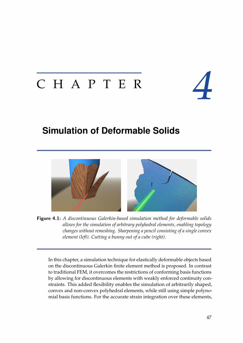
C H A P T E R 4Simulation of Deformable Solids
Figure 4.1: A discontinuous Galerkin-based simulation method for deformable solidsallows for the simulation of arbitrary polyhedral elements, enabling topologychanges without remeshing. Sharpening a pencil consisting of a single convexelement (left). Cutting a bunny out of a cube (right).
In this chapter, a simulation technique for elastically deformable objects basedon the discontinuous Galerkin finite element method is proposed. In contrastto traditional FEM, it overcomes the restrictions of conforming basis functionsby allowing for discontinuous elements with weakly enforced continuity con-straints. This added flexibility enables the simulation of arbitrarily shaped,convex and non-convex polyhedral elements, while still using simple polyno-mial basis functions. For the accurate strain integration over these elements,
47

Simulation of Deformable Solids
an analytic technique based on the divergence theorem is presented. Beingable to handle arbitrary elements eventually allows for simple and efficienttechniques for volumetric mesh generation, adaptive mesh refinement, androbust cutting. Furthermore, the presented DG method does not to sufferfrom locking artifacts even for nearly incompressible materials, a problemthat in standard FEM requires special handling.
After having introduced the main concepts of DG FEM based on a simple 2DPoisson problem in Section 3.1, this chapter shows how to derive equationsand techniques for 3D linear elasticity (Section 4.2). DG FEM is extended fur-ther by directly simulating arbitrary polyhedra (Section 4.3), by generalizingstiffness warping to DG FEM (Section 4.4), and by using embedded simula-tion (Section 4.5) with suitable collision handling (Section 4.6). Equipped withthose techniques, the versatility of the presented framework is demonstratedon a set of different applications in Section 4.7.
4.1 Overview
In computer graphics, FEM simulations of deformable objects are usuallybased on simple tetrahedral or hexahedral meshes. To simulate topologicalchanges due to cutting or fracturing of material, one has to split elements andperform a remeshing step in order to avoid ill-shaped elements and to main-tain a reasonable mesh quality. Due to the relaxed conformity constraints, aDG FEM-based approach allows for arbitrary convex and non-convex poly-hedral elements, which greatly simplifies the mesh restructuring step. In thecontext of cutting and fracturing the approach presented in this work is mostsimilar to Wicke et al. [2007] and Martin et al. [2008], but it is more flexibleand more efficient due to the use of simple polynomial shape functions.
Furthermore, in order to support flexible simulations of deformable mod-els for computer graphics applications, this work extends DG FEM by thefollowing components:
• The simulation of arbitrary polyhedral elements using simple and ef-ficient polynomial basis functions and a fast and accurate volumetricintegration technique (Section 4.3).
• A generalization of stiffness warping to discontinuous polyhedralelements, thereby allowing linear strain measures to be used even inthe presence of large deformations (Section 4.4).
• For embedded simulations: the reconstruction of a smooth displace-ment field from the discontinuous mesh, based on moving least
48

4.2 Linear Elasticity using DG FEM
squares (MLS) interpolation (Section 4.5), along with a suitable colli-sion handling technique (Section 4.6).
The versatility of the presented approach is demonstrated on several exam-ples, including slicing-based mesh generation, adaptive stress-based elementrefinement, flexible and efficient cutting, and locking analysis (Section 4.7).
4.2 Linear Elasticity using DG FEM
The basic concepts of DG FEM have been introduced on the 2D Poissonproblem in Section 3.1.2. Based on this introduction, this section shows howthe same approach can be applied to the simulation of 3D linearly elasticdeformations as presented in Section 3.4.
4.2.1 DG Weak Form
The derivation of the DG weak form for linear elasticity closely follows theprocedure presented in Sections 3.1.2 and 3.1.3, where the derivation of aDG method for the 2D Poisson problem has been shown. Equations (3.28)and (3.29), which constitute the strong form of elastostatics, are multiplied bytest functions and integrated over each element K, yielding the individualelements’ weak forms. Those are summed up, fluxes u and σ are introduced,and the two resulting equations are combined into one. The resulting equa-tion corresponds to (3.11) for the Poisson problem, and is to be simplifiedusing the average and jump operators.
Those, however, have to be slightly redefined for vector-valued functions uand matrix-valued functions σ on a face f shared by two elements K− andK+, such that the jump operator maps vectors to matrices and vice versa.Using the outer product u⊗ n := unT we define
u :=12(u− + u+
), JuK := u− ⊗ n− + u+ ⊗ n+,
σ :=12(σ− + σ+
), JσK := σ−n− + σ+n+.
BZ Method. Minimizing the jump JuK : JuK = ‖u− − u+‖2 by choosing thefluxes of Babuska and Zlamal [1973] leads to the weak form of the BZ method,which uses aBZ instead of aCG in (3.30):
aBZ(u,v) :=∫
Ωε(v) :C : ε(u) +
∫Γ
η f JuK : JvK . (4.1)
49

Simulation of Deformable Solids
Figure 4.2: Comparison between CG FEM (left), DG FEM (center), and the elasticallycoupled rigid cells of PriMo (right). The DG method conceptually spansthe whole space from CG to PriMo, since for sufficiently large penalties η itapproximates the CG results, and for an extremely stiff material and lowerpenalty η it reproduces the rigid cells of PriMo.
The penalty parameter η f is defined per face f according to Hansbo and Lar-son [2002]:
η f = η · area( f ) ·(
1vol(K−)
+1
vol(K+)
)(4.2)
using a global penalty parameter η > 0, which was typically in the order of101–102 for the simulations shown in this work.
The internal elastic energy of the deformed object can then be written as
aBZ(u,u) =∫
Ωσ(u) : ε(u) +
∫Γ
η f∥∥u− − u+
∥∥2 ,
which reveals an interesting connection to both CG FEM and the elasticallycoupled rigid cells of PriMo [Botsch et al., 2006]: CG computes elastic energieswithin elements only, using the Ω-integral, whereas PriMo employs only the“glue” energy between elements, represented by the Γ-integral.
Since BZ is based on both energy terms, with properly chosen penalty weightand material stiffness it can reproduce both methods, and can hence beconsidered as their generalization (see Fig. 4.2). As such, it combines thestrengths of both approaches, since it inherits the physical accuracy of CGFEM, as well as the flexibility in element shapes and meshing of PriMo [Botschet al., 2007], as will be demonstrated in Section 4.3.
The BZ penalty term is equivalent to both the glue energy of PriMo [Botsch etal., 2006] and the soft bindings employed by Sifakis et al. [2007b]. However,as already discussed in Section 3.1.3 and shown in Fig. 3.7, the BZ methodis not consistent and therefore does not provide any convergence guarantees.Our experiments have nevertheless shown the BZ method to be very wellsuited for applications aiming at physically plausible deformations only.
50

4.2 Linear Elasticity using DG FEM
IP Method. However, if physical accuracy is important, other DG fluxes,such as those of the IP method, should be chosen instead. For linear elasticity,the weak form of the IP method [Douglas and Dupont, 1976] is defined by
aIP(u,v) :=∫
Ωε(v) : C : ε(u) (4.3)
−∫
Γ
(JvK :σ(u)
+ JuK :σ(v) − η f JuK : JvK).
A detailed derivation of this weak form can be found in Section A.1.
Analogous to the Poisson problem (3.16), the three penalty terms ensure con-sistency, symmetry, and stability, and the method is guaranteed to convergeunder element refinement. Moreover, the IP method is still relatively easy toimplement (see Section 4.2.2). While other (more complex) numerical fluxesexist (e.g., Ten Eyck and Lew [2006], Wihler [2006]), for our applications theBZ and IP methods performed very well and have been fully sufficient.
4.2.2 Discretization and Matrix Assembly
Discretization. To implement DG FEM for linear elasticity, we discretize uand v using n basis functions and set up the stiffness matrix K:
u(x) ≈n
∑i=1
uiNi(x) with ui ∈ IR3, (4.4)
v(x) ≈n
∑i=1
viNi(x) with vi ∈ IR3. (4.5)
Note that in this context, x ∈Ω ⊂ IR3 denotes a position in the undeformedconfiguration. Since this is very similar to CG FEM, the reader is referredto Hughes [2000] and Nealen et al. [2006] for more details on the followingderivations.
Using a 3× 3n interpolation matrix H(x) built from the basis functions Ni(x)
H(x) =
N1(x) 0 0 N2(x) 0 00 N1(x) 0 0 N2(x) 0 . . .0 0 N1(x) 0 0 N2(x)
and a 3n vector U containing the unknown coefficients ui ∈ IR3, the discretiza-tion (4.4) of u can be written in matrix notation as u(x) =H(x)U. Equivalently,the test function v can be represented as v(x) = H(x)V.
51

Simulation of Deformable Solids
Moreover, using Voigt notation, stress and strain can be represented by 6Dvectors σ and ε composed of the independent entries of the symmetric 3× 3matrices σ and ε (defined in Equations (3.27) and (3.28)), respectively:
σ(u) = (σ11, σ22, σ33, σ23, σ13, σ12)T,
ε(u) = (ε11, ε22, ε33, 2ε23, 2ε13, 2ε12)T.
This leads to the matrix notation of the linear stress-strain relationship
σ(u(x)) = C ε(u(x)) = CB(x)U, (4.6)
with a constant symmetric 6× 6 matrix C built from the coefficients of theconstitutive tensor C (see Eq. (3.26)),
C =
2µ + λ λ λ 0 0 0λ 2µ + λ λ 0 0 0λ λ 2µ + λ 0 0 00 0 0 µ 0 00 0 0 0 µ 00 0 0 0 0 µ
,
and a 6× 3n matrix B(x) containing first derivatives of the basis functions Ni:
B(x) =
N1,1(x) 0 0 N2,1(x) 0 00 N1,2(x) 0 0 N2,2(x) 00 0 N1,3(x) 0 0 N2,3(x) . . .0 N1,3(x) N1,2(x) 0 N2,3(x) N2,2(x)
N1,3(x) 0 N1,1(x) N2,3(x) 0 N2,1(x)N1,2(x) N1,1(x) 0 N2,2(x) N2,1(x) 0
For the assembly of the stiffness matrix we use the above matrix notationsto write the IP weak form (4.3) in terms of element contributions (Ω-integrals)and face contributions (Γ-integrals). Note that for the BZ method (4.1) only thelast of the three face contributions in (4.3) is needed.
The element contributions are written in terms of element stiffness matricesKK as in CG FEM: ∫
Ωε(v) :C : ε(u) = ∑
K∈TVTKKU (4.7)
with KK =∫
KBT(x) CB(x) .
52

4.2 Linear Elasticity using DG FEM
After expanding the operators · and J·K, and exploiting n−= −n+, the firsttwo face contributions of f = K− ∩ K+ have the form
JvK :σ(u) =((
v+ − v−)⊗ n+
):
12(σ−(u) + σ+(u)
).
To write this in matrix notation, we need a 6× 3 matrix
N f :=
n+1 0 0 0 n+
3 n+2
0 n+2 0 n+
3 0 n+1
0 0 n+3 n+
2 n+1 0
T
,
and differences and averages of matrices B and H
HJKf :=
(H+
f −H−f)
, Bf :=12
(B+
f + B−f)
,
which themselves are defined through restrictions
B±f := B|K± , H±f := H|K± ,
containing only the entries of B or H corresponding to basis functions of K±.
With these matrices we can define three stiffness matrices K f 1, K f 2, and K f 3for each face f :
K f 1 =∫
f−HJK
fT
NTf CBf ,
K f 2 =∫
f−Bf
TCN f HJK
f ,
K f 3 =∫
fη f HJK
fT
HJKf .
The three face contributions in (4.3) can now be written in terms of these facestiffness matrices as
−∫
ΓJvK : σ(u) = ∑
f∈TVTK f 1 U, (4.8)
−∫
ΓJuK :σ(v) = ∑
f∈TVTK f 2 U, (4.9)
∫Γ
η f JuK : JvK = ∑f∈T
VTK f 3 U. (4.10)
The global 3n× 3n stiffness matrix K can therefore be assembled by doingone pass over all elements K ∈ T and accumulating their contributions KK,
53

Simulation of Deformable Solids
and a second pass over all faces f ∈ T that accumulates their contributionsK f i. Equivalently to CG, the external force vector F is assembled from theelements’ contributions
∫K H(x)T f. Note that even for linear basis functions
the integrands H(x) are not constant, requiring integration techniques asdiscussed in Section 4.3. The discretized weak form
VTKU = VTF
has to hold for all test functions v, i.e., all vectors V, leading to the linearsystem KU = F to be solved for the static solution U.
Assembly. The assembly of element and face stiffness matrices into theglobal stiffness matrix K can be formulated most easily in terms of individual3× 3 matrices. Let KK[i,j] denote the 3× 3 submatrix of KK corresponding tothe global stiffness matrix entry Kij. The matrices KK[i,j] can be precomputedfor all elements K using (4.7), and only those matrices that are non-zero needto be stored. Due to symmetry it holds that KK[i,j] = KK[j,i]
T, which furtherreduces the number of matrices to be precomputed. Similarly, K f 1[ij] andK f 3[ij] can be precomputed for all faces f . Note that K f 3[ij] = K f 3[ji]
T andK f 2[ij] = K f 1[ji]
T, so K f 2 does not need to be precomputed explicitly.
Kij can now be defined in terms of element and face contributions as follows:
Kij = ∑K
KK[ij] + ∑f
(K f 1[ij] + K f 1[ji]
T + K f 3[ij]
).
Using a notation where the operator ← denotes assembly into the globalstiffness matrix for all K, f , this can equivalently be written as:
Kij← KK[ij]
Kij← K f 1[ij]
Kji← K f 1[ij]T
Kij← K f 3[ij]
Boundary Conditions. Dirichlet boundary constraints can be prescribed inDG FEM as weak or strong constraints. The latter simply removes someDOFs from the system, i.e., fixes the coefficients ui for the corresponding Ni.Weak boundary conditions are imposed by appropriately defining averagesand jumps at boundary elements. For a prescribed displacement g this meansto define the function values on the “free” side of boundary faces f ∈ ∂Ω as
u− := g, σ−(u) := σ+(u) ,v− := 0, σ−(v) := σ+(v) .
54
4.3 Arbitrary Polyhedral Elements
Time Integration. Dynamic simulations of deformable objects with time-varying U(t) and F(t) require additional inertial and damping forces, result-ing in the governing equations
MU + DU + KU = F, (4.11)
with mass matrix M and damping matrix D, equivalent to CG FEM [Nealenet al., 2006]. The 3× 3 submatrices of the mass matrix M can be computed as
Mij = ρ∑K
∫K
Ni(x)Nj(x) I3,
where ρ is the uniform density of the object. The damping matrix D is usuallycomputed as a linear combination of the stiffness matrix K and the massmatrix M.
In order to guarantee stability a semi-implicit Euler time-integration isemployed: Integrating the system forward in time from state (Uk,Uk) to(Uk+1,Uk+1) using a time step size ∆t, the new DOFs and their accelerationare expressed in terms of the new velocities as
Uk+1 ≈ Uk + Uk+1∆t,
Uk+1 ≈Uk+1 − Uk
∆t,
resulting in Uk+1 being the only unknown for time step k + 1. Formulatingthe governing equations (4.11) for time step k + 1 and reordering the resultingterms gives the sparse, symmetric, positive definite linear system
(K∆t2 + D∆t + M) Uk+1 = (F−KUk)∆t + MUk (4.12)
to be solved for Uk+1 in each time step, from which in turn the values of theDOFs Uk+1 can be computed.
Two kinds of linear system solvers were applied to the resulting equations:preconditioned conjugate gradients [Saad and van der Vorst, 2000] and sparseCholesky factorization [Toledo et al., 2003]. While both worked well in allthe experiments performed, the Cholesky solver turned out to scale betterto larger problems thanks to its quasi-linear asymptotic complexity, as alsoobserved in Botsch et al. [2005].
4.3 Arbitrary Polyhedral Elements
The main advantage of DG FEM is the possibility to use non-conforming,discontinuous shape functions Ni. This added flexibility allows us to em-ploy simple degree-k polynomials 1, x,y,z, xy, . . . ,zk as (non-nodal) basis
55

Simulation of Deformable Solids
Figure 4.3: Examples of possible element shapes include the common tetrahedral andhexahedral elements (left), as well as arbitrary convex and non-convex poly-hedra (middle). It is even possible to treat the whole simulation domain asone single element (right).
functions within each element K. In this work, either 4 linear or 10 quadraticbasis functions were used per element. Notice that k should be ≥ 1, sincethen the DG method can exactly reproduce rigid motions, yielding a linear,continuous displacement function u without jumps [Cockburn, 2003].
In contrast to nodal basis functions, these non-nodal basis functions no longerdepend on the element shape, thereby enabling us to work with arbitrar-ily shaped elements. For practical reasons, however, element shapes arerestricted to convex or non-convex polyhedra (i.e., planar faces and linearedges, see Fig. 4.3), which still is considerably more flexible than the convexpolyhedra with triangulated faces of Wicke et al. [2007]. Compared to theharmonic shape functions of Martin et al. [2008], which also allow for non-convex elements, our polynomial basis functions are simpler and thereforemore efficient to compute.
For a practical implementation we have to accurately and efficiently computeintegrals of the form∫
KNaNb,
∫K
∂Na
∂xi
∂Nb∂xj
,∫
fNaNb,
∫f
∂Na
∂xiNb,
over elements K and faces f , since they are the building blocks for the matrixassembly described in Section 4.2.2. While tetrahedra or hexahedra canbe integrated analytically, general polyhedral elements with nodal basisfunctions typically require numerical integration, which trades accuracyfor performance [Wicke et al., 2007]. In contrast, as will be shown in thefollowing section, polynomial functions can be integrated analytically over apolyhedron. By using polynomial basis functions, all of the aforementionedelement integrals can thus be computed exactly up to numerical round-offerrors.
56

4.3 Arbitrary Polyhedral Elements
𝑝(𝒙)𝐾
= …𝑓𝑓∈𝜕𝐾
= …𝑒𝑒∈𝜕𝑓𝑓∈𝜕𝐾
= 𝑔(𝒑1,… , 𝒑𝑛)
Figure 4.4: The basic idea of divergence theorem-based volume integration: an integralover a polyhedron K is reduced to a sum of area integrals, a sum of lineintegrals, and finally becomes a function of the polyhedron’s nodal positions.
4.3.1 Divergence Theorem Integration
Using the divergence theorem, the volume integral of a degree-k polynomialp over an element K can be reduced to an area integral of a degree-(k + 1)polynomial q over its boundary ∂K, i.e., to a sum of integrals over its faces.Each face integral can in turn be reduced to line integrals over its edges e ∈ ∂ f ,which in the end results in degree-(k + 3) polynomials in the edge endpoints(see Fig. 4.4).
Divergence Theorem. For a function f : IR3→ IR and a constant 3-vector dthe following variant of the divergence theorem holds:∫
Ω∇ f · d dΩ =
∫Γ
f d · n dΓ, (4.13)
where Ω is a volume bounded by the surface Γ. (4.13) also holds if Ω is aplanar surface in IR3 and Γ is the boundary of that surface. In this case, dmust be orthogonal to the normal of the surface.
Volume Integration. We want to integrate a function p : IR3 → IR over apolyhedral volume element K
J =∫
Kp(x) dx
with x = (x1, x2, x3)T. Assuming the existence of a function q : IR3→ IR and a
non-zero vector d with the property p(x) =∇q(x) · d, the integrand can besubstituted. Applying the divergence theorem (4.13) gives
J =∫
K∇q(x) · d dx =
∫Γ
q(x) d · n dA = ∑f∈∂K
∫fq(x) dA d · n f (4.14)
57

Simulation of Deformable Solids
where n f is the outward unit normal vector of element face f . Using the (yetto be defined) function q and vector d, we are thus able to express the volumeintegral of a function p as a sum of surface integrals of a function q.
Surface Integration. To transition from surface integrals to line integrals,we start with the integral of a function q : IR3→ IR over a planar face f :
I =∫
fq(x) dA.
Let n f = (n f1 ,n f
2 ,n f3)
T be the unit normal of the face. We assume that theboundary of the face consists of m straight edges, where the e-th edge connectsnodes pe and pe+1, e ∈ 1, . . . ,m, and pm+1 := p1. The plane equation of f isx · n f − C = 0 with C := p1 · n f .
Following Mirtich’s [1996] approach of projecting surface integrals ontocoordinate planes, the face f is projected onto either the x1 = 0, x2 = 0 orx3 = 0 plane, depending on the face’s orientation. We want the projected faceto have non-zero area, thus it is reasonable to use the maximum componentof n f as the direction of projection, i.e. to project face f onto the xd = 0plane with d = argmaxi |n f
i |. Let the unit vector ed = (δ1d,δ2d,δ3d)T denote
the direction of projection where δij is the Kronecker delta.
A point x = (x1, x2, x3)T on f is projected to x = (x1, x2, x3)
T on f with
xi = (1− δid)xi.
Using the plane equation of f , the inverse mapping (from x to x) can be foundto be
xd =C− xd+1n f
d+1 − xd+2n fd+2
n fd
,
xd+1 = xd+1,xd+2 = xd+2,
where the indices of x and x are assumed to wrap around, i.e. x4 := x1,x5 := x2, and so on.
The integral I can now be computed as
I =1
|n fd |
∫fq(x) dx with q(x) := q(x(x)).
58

4.3 Arbitrary Polyhedral Elements
Assuming the existence of a function r : IR3 → IR and a non-zero vector dsatisfying q(x) =∇r(x) · d and ed · d = 0, the divergence theorem (4.13) canbe applied to the projected face f :
I =1
|n fd |
∫f∇r(x) · d dx =
1
|n fd |
∑e∈∂ f
∫er(x)ds d · ne.
Here, the integral over the boundary of f has been replaced by a sum overintegrals over the projected face’s edges e. ne is the outward unit normal ofedge e on the projection plane.
Line Integration. As all edges are assumed to be straight, they can beparameterized as
x(t) = pe(1− t) + pe+1t
with 0≤ t ≤ 1 and projected nodes pe. The integral becomes
I =1
|n fd |
∑e∈ f
le∫ 1
0r(x(t))dt d · ne
where le := ||pe+1 − pe|| is the length of the projected edge e. The normal ofthe projected edge e can be found to be
ne =1le
sign(n fd)(pe+1 − pe)× ed.
The factor sign(n fd) is required in order to ensure that the normal of the
projected edge is always pointing outwards. The integral now simplifies to
I =1
n fd
∑e∈ f
∫ 1
0r(x(t))dt (pe+1 − pe) · (ed × d) (4.15)
where we have made use of the fact that pe · (ed × d) = pe · (ed × d).
Volume to Nodal Positions. Using (4.15) to compute the face integral in(4.14) finally gives a closed form for the computation of J =
∫K p(x):
J = ∑f∈∂K
1
n fd
∑e∈ f
(∫ 1
0r(x(t))dt
)(pe+1 − pe) · (ed × d)(d · n f ) (4.16)
If p is a polynomial in x, q can be computed by integrating p in direction xd,then substituting x for x in q to get q. Integration of q in direction d givesr(x). Parameterizing x with t and analytically computing the integral
∫ 10 then
results in a polynomial in pe and pe+1. The integral (4.16) thus evaluates to apolynomial in the nodal positions of the polyhedral element K.
59

Simulation of Deformable Solids
4.3.2 Integration Algorithm
The following steps show how to compute∫
K p(x)dx for an arbitrary polyno-mial p(x) with x = (x1, x2, x3)
T.
1. Integrate p(x) formally to obtain the polynomial q(x) in x:
q(x)←∫
p(x)dx1
2. Perform the following three steps for i ∈ 1,2,3, with j and k definedas j = (i mod 3) + 1 and k = ((i + 1) mod 3) + 1.
a) Transform q(x) into the polynomial q(x,n) in x = (x1, x2, x3)T
with the symbolical constant n = (n1,n2,n3)T by performing the
following substitutions:
xi→1ni− xj
nj
ni− xk
nkni
,
xj→ xj,
xk→ xk
b) Integrate q(x,n) formally to obtain the polynomial r(x,n) in x:
r(x,n)←∫
q(x,n)dxj
c) Integrate formally over the edge connecting a = (a1, a2, a3)T and
b = (b1,b2,b3)T to get a polynomial in a and b:
Pi(a,b,n)← (bk − ak)∫ 1
0r(a (1− t) + b t,n)dt
3. The integral over the volume can now be computed as follows, wheren f = (n f
1 ,n f2 ,n f
3)T defines the plane of face f as x ∈ IR3|x · n f = 1.
d f ∈ 1,2,3 is the direction of projection for face f which must be
chosen such that n fd f6= 0. ae and be are the start and end points of
edge e. ∫K
p(x)dx = ∑f∈∂K
n f1
n fd f
∑e∈∂ f
Pd f(ae,be,n f )
In a practical implementation, a code generation tool would be used to createthe code for computing the polynomials Pi, i ∈ 1,2,3, for one particularpolynomial p(x).
60

4.4 Stiffness Warping
10−4
10−2
100
102
104
10−15
10−10
10−5
100
Duration [ms]
Err
or
Uniform SamplingMonte−Carlo IntegrationDivergence Theorem
Figure 4.5: Comparison of different numerical integration methods to the analytic methodbased on the divergence theorem. In this example the function f (x,y,z) = x2
was integrated over the corner-cut cube model shown on the right.
4.3.3 Evaluation
Fig. 4.5 compares the analytic integration to different numerical schemesin terms of accuracy and performance. While the method based on thedivergence theorem is exact up to round-off errors, it is also reasonablyefficient: a straightforward numerical integration still shows an error of about10−2 for the same computation time. Compared to CG FEM using the meanvalue polyhedral elements of Wicke et al. [2007], the exact integration methodis faster by an order of magnitude.
4.4 Stiffness Warping
Under large rotational deformations, linear FEM shows artifacts such as anunrealistic increase in volume. To avoid the cost of a full nonlinear simulationbut still get physically plausible deformations in these cases, a corotatedformulation can be employed, which computes elastic forces in a rotatedcoordinate frame defined for each element [Muller and Gross, 2004; Hauthand Strasser, 2004].
In linear CG FEM, the forces acting on the nodes of an element K are com-puted from nodal displacements U and the element stiffness matrix KK de-fined in (4.7) as follows:
FK = KKU = KK
(X− X0
), (4.17)
61

Simulation of Deformable Solids
with X and X0 denoting the deformed and undeformed nodal positions,respectively. In order to avoid the aforementioned rotational artifacts, thecorotational, or warped stiffness approach [Muller and Gross, 2004; Hauth andStrasser, 2004] first reverts the element’s rotation, computes displacementsand forces in the un-rotated state, and re-rotates the resulting forces:
FK = RK KK
(RT
KX− X0)
, (4.18)
where RK is a block-diagonal matrix containing the 3× 3 rotation matrix ofelement K on its diagonal.
This approach cannot be directly applied to DG for two reasons. First, thecontributions resulting from integrals over interior faces are associated withtwo elements and require special treatment. Second, in case non-nodal basisfunctions are used, we will no longer be solving for nodal displacements, andX0 in (4.17) needs to be generalized to a set of degrees of freedom definingthe undeformed state of the object in terms of the basis functions Ni.
4.4.1 Element and Face Contributions
Element contributions (4.7) can be treated just as in CG FEM using (4.18).We determine the rotations of general polyhedra by first fitting an affinetransformation to the nodal displacements in the least squares sense, and thenextracting its rotational component RK using polar decomposition [Hauthand Strasser, 2004].
Note that for face contributions (4.8), (4.9), (4.10) we cannot simply apply(4.18) using the face’s rotation, since that would lead to ghost forces andinstabilities similar to the per-vertex stiffness warping of [Muller et al., 2002].Moreover, the corotational method is only required to correct artifacts due tolinear strain ε = BU, and hence is not needed for (4.10).
For the face contributions (4.8) and (4.9) it is crucial that the strains B+f U and
B−f U, which constitute Bf , are computed consistently with the strains of theelement contributions (4.18) of K+ and K−. This requires to use the elements’rotations R+
f and R−f for correcting B+f U and B−f U, respectively. We therefore
have to split up the stiffness matrices K f 1 and K f 2 w.r.t. strain contributionsfrom either K+ or K−, yielding the four stiffness matrices
K±f 1 := −12
∫fHJK
fT
NTf CB±f ,
K±f 2 := −12
∫fB±f
TCN f HJKf ,
62

4.4 Stiffness Warping
where (·)± again denotes either (·)+ or (·)−. These stiffness matrices allowfor a consistent warping of a face f ’s contributions, such that we get fivecorotated contributions:
F±f 1 = R±f K±f 1
(R±f
TX− X0)
,
F±f 2 = R±f K±f 2
(R±f
TX− X0)
,
F f 3 = K f 3(X− X0) .
4.4.2 Non-Nodal Basis Functions
In order to use stiffness warping for non-nodal basis functions, we needto generalize the definition of the vector X0 representing the undeformedstate. To this end, we have to find x0 = (x0
1T, . . . ,x0
nT)T satisfying the identity
∑i X0i Ni(x) ≡ x. For nodal basis functions, this vector would contain the
nodal positions of the undeformed mesh. Since for each element K our non-nodal basis functions always contain the linear polynomials (see Section 4.3),finding X0 is trivial. For each element K, if its linear basis functions are
NiK(x) = x, NjK(x) = y, NkK(x) = z,
we simply set the corresponding coefficients to
x0iK = (1,0,0)T, x0
jK = (0,1,0)T, x0kK
= (0,0,1)T,
and use x0lK= (0,0,0)T for all its other basis functions. This results in a vector
X0 representing the undeformed state, based on which stiffness warping canbe performed just as for nodal basis functions.
Note that for quadratic or higher order basis functions, stiffness warpingonly removes the global element rotation, whereas local rotations due tobending might remain. While this was not a problem in all of the experimentsperformed, such cases can easily be detected and the respective elements canbe refined (see Section 4.7).
4.4.3 Warped Assembly
To formulate the assembly of the stiffness matrix (see Section 4.2.2) in thepresence of stiffness warping, we need to first split up (4.18) into a termproportional to U and a static force term as follows:
RK KK RTK U = FK + RK KK (I3n −RT
K)X0.
63

Simulation of Deformable Solids
Every time the element rotations change, the warped element contributionsare to be re-assembled as follows:
Kij← RK KK[ij] RTK
Fi← RK KK[ij] (I3 −RTK)X
0j
Note that contrary to the notation used previously, RK and R±f denote 3× 3rotation matrices here. The face contributions are assembled as follows:
Kij← R±f K±f 1[ij] R±f
T
Fi← R±f K±f 1[ij] (I3 −R±fT)X0
i
Kji← R±f K±f 1[ij]T R±f
T
Fj← R±f K±f 1[ij]T(I3 −R±f
T)X0
j
Kij← K f 3[ij]
4.5 MLS-Based Surface Embedding
When it comes to the simulation of complex models, a common approachfor keeping computation costs low is to embed a high resolution surfacemesh into a lower resolution simulation mesh. The latter can be simulatedefficiently, and its displacement field u(x) is used to deform the surface mesh[Faloutsos et al., 1997; Muller et al., 2004b; James et al., 2004; Sifakis et al.,2007b]. In DG FEM, the discontinuous displacement u cannot be applieddirectly to the high resolution surface, since it would lead to gaps and self-intersections.
In a first step, discontinuities are removed by stitching the simulationmesh. For each node x0
i ∈ T , the average of its different displacementsu|K(x0
i)
corresponding to its incident elements K ∈ Ni is computed, similarto Botsch et al. [2006]:
ui =1|Ni| ∑
K∈Ni
u|K(
x0i
). (4.19)
This results in a deformed, continuous simulation mesh, which is sufficientfor visualizing the simulation mesh itself.
The averaged nodal displacements have to be interpolated within elements inorder to deform the embedded mesh. For tetrahedral or hexahedral elementsthis amounts to simple linear or trilinear interpolation, respectively. For more
64

4.5 MLS-Based Surface Embedding
Figure 4.6: Comparison of embedding techniques. Stitching the discontinuous simula-tion mesh, followed by barycentric interpolation, leads to C0 artifacts (left). Incontrast, the presented smooth MLS-based embedding yields a considerablyhigher surface quality (right).
general convex or non-convex polyhedra, mean value coordinates [Floateret al., 2005; Ju et al., 2005] or harmonic coordinates [Joshi et al., 2007] canbe employed. All these methods, however, correspond to a non-smooth,generalized barycentric C0 interpolation, resulting in clearly visible shadingartifacts for coarse simulation meshes (see Fig. 4.6, left).
Botsch et al. [2007] employ globally supported radial basis functions for highquality interpolation, but the involved dense linear systems are prohibitive forcomplex simulation meshes. To overcome these limitations, and inspired bymeshless methods [Muller et al., 2004a; Pauly et al., 2005], this work proposesa smooth embedding based on moving-least-squares (MLS) interpolation.
If we denote by x0i the nodes of the undeformed simulation mesh, and by ui
their averaged displacements, then the displacement at a material point x iscomputed by fitting an affine transformation, which amounts to minimizingthe weighted least square error
Emls(x) =12 ∑
iθ(∥∥∥x− x0
i
∥∥∥) ∥∥∥C(x)T p(
x0i
)− ui
∥∥∥2, (4.20)
with p(x,y,z) = (1, x,y,z)T and θ(d) a (truncated) Gaussian weightfunction. Computing ∂Emls/∂p = 0 results in a 4 × 4 linear systemA(x)C(x) = b(x) that yields the coefficients C(x) for the interpolated dis-placement u(x) = C(x)T p(x) at the position x. This MLS-based embeddinghas several interesting properties:
• The smoothness of the interpolation is determined by the weightingkernels θ, resulting in a high quality embedding for our choice ofGaussian kernels (see Fig. 4.6, right).
65

Simulation of Deformable Solids
• The use of linear polynomials p(x), in combination with the parti-tion of unity property of MLS shape functions, guarantees the exactreproduction of linear displacements u, i.e., in particular of rigidmotions [Fries and Matthies, 2004].
• Since the approach is entirely meshless it can be used to interpolatewithin arbitrarily shaped elements. Choosing the support radius ofθ proportional to the local sampling density at x0
i (e.g., distances toone-ring neighbors), yields smooth interpolations even for irregularmeshes.
• An accurate approximation of higher order polynomial displacementsu only requires to add more samples (x0
i , ui) to (4.20), such as edge,face, or element midpoints.
• The interpolated displacement u(x) of a vertex x of the embeddedmesh linearly depends on C(x), which in turn linearly depends on theui used in (4.20), which finally linearly depend on ui through (4.19)and (4.4). Hence, by combining these linear relationships, the weightsθ(∥∥x− x0
i
∥∥) as well as the set N (x) of relevant basis functions Ni canbe precomputed, such that during the simulation only
u(x) = ∑i∈N(x)
θ(∥∥∥x− x0
i
∥∥∥)Ni(x)ui =: ∑i∈N(x)
Wi(x)ui (4.21)
has to be evaluated as a linear combination of the DOFs ui.
4.6 Collisions
Since collision handling is not the focus of this work, it has been restrictedto simple penalty-based collision response within the semi-implicit timeintegration. The basic approach is equivalent to CG FEM, therefore only thedifferences due to the discontinuous displacement field u are discussed here.
Suppose that in the current time step we detect a collision at a displacedmaterial point xc + u(xc). Since we use the interpolated displacement u of(4.21), xc can be an arbitrary embedded point, e.g., a vertex of the embeddedsurface mesh. Nodal collisions using the stitched displacement (4.19) is just aspecial case of this formulation.
For collision response a penalty force proportional to the penetration depth isadded to the system. Consider an oriented collision plane with outward unit
66

4.6 Collisions
Figure 4.7: Collision handling on the nodes of the simulation mesh (left) and the verticesof the embedded mesh (right).
normal vector n and p being an arbitrary point on the plane. The penetrationdepth d can be computed as
d = p · n− (xc + u(xc)) · n.
Defining a collision force proportional to the penetration depth yields
f(xc) = k dn = Au(xc) + b
with A =−k nnT and b = k nnT(p− xc), where k is the collision penalty. Thisforce is used in the semi-implicit solver whenever d > 0. The correspondingpenalty energy is
Ecoll(xc) =12
u(xc)T Au(xc) + u(xc)
T b,
which after inserting the definition of u in (4.21) becomes
12 ∑
i,juT
i Wi(xc)AWj(xc)uj + ∑i
uTi Wi(xc)b.
Since this collision energy corresponds to an external force, it has to be eithersubtracted from the internal potential energy 1
2UTKU or to be added to theexternal energy UTF. Hence, we can incorporate the collision energy Ecollinto the system (4.11) by updating 3× 3 blocks of the stiffness matrix K and3-vectors of the external force F (see Section 4.2.2):
Kij −= Wi(xc)AWj(xc) ,
Fi += bWi(xc) ,
for all i, j ∈ N (xc), i.e., the set of basis functions Wi, respectively Ni, influenc-ing the collision point xc (see (4.21)).
67

Simulation of Deformable Solids
Method Resolution #DOFs Spars. Int. Ass. SolveBZ lin. 10×10×10 12k 0.28% 532 22 656IP lin. 10×10×10 12k 0.62% 1437 87 734CG trilin. 15×15×15 12k 0.58% 3750 41 641BZ quad. 10×10×10 30k 0.28% 3062 152 7797IP quad. 10×10×10 30k 0.64% 8344 621 8484
Table 4.1: Comparison of BZ and IP with linear/quadratic basis functions to trilinearCG FEM for 3D elasticity. The mesh resolution is chosen to match the DOFsof DG and CG. The table lists matrix sparsity and timings (in ms) for volumeintegration, matrix assembly, and the solution of the linear system (taken onan Intel Core2 Duo 2.4 GHz).
If the simulation mesh is also used for visualization, simple nodal collisionsare sufficient in most cases, as for instance for the examples shown in Sec-tion 4.7. However, for embedded simulations collisions should be detectedand handled on the vertices of the embedded surface (see Fig. 4.7).
4.7 Results
This section demonstrates how the possibility to use arbitrary polyhedralelements and simple polynomial shape functions can be exploited to derivea versatile and efficient simulation technique. Before presenting specificexample applications, the general advantages and disadvantages of DG FEMcompared to CG FEM are discussed.
DG FEM versus CG FEM for Linear Elasticity. A quantitative comparisonbetween CG and DG using BZ/IP penalties and linear/quadratic basis func-tions, based on a 2D Poisson problem with analytically known solution hasalready been shown in Chapter 3, see Fig. 3.8. In addition, Table 4.1 givessome statistics and timings of the same five methods for 3D linear elasticity.Note that even for the same mesh and basis functions DG provides moredegrees of freedom (DOFs) than CG, since nodes can “split” due to discon-tinuous displacements. The plots and timings are therefore with respect toDOFs.
The only additional parameter compared to CG FEM is the penalty weightη in (4.2), (4.3), which has to be sufficiently high to guarantee stability. Onesimple strategy to find a suitable penalty is to start with a low value anddouble it until K is positive definite. This worked well for all experimentsperformed in the context of this work and typically leads to η in the order
68

4.7 Results
Figure 4.8: Intersecting the bunny with a hex-grid generates 41 elements (left). Closeupview of a non-convex element (right).
of 101–102. Note that η should not be too high, since otherwise the methodresembles CG and does not exploit its additional DOFs (Fig. 4.2).
The missing consistency terms of BZ (see (4.1), (4.3)) allow for sparser matri-ces and higher efficiency. Furthermore, the method is stable for any positivepenalty η. Although lacking theoretical convergence guarantees, BZ shows areasonable convergence behavior in practice and gives visually convincingresults. We therefore consider it well suited for typical graphics applica-tions requiring physically plausible deformations only. For more accuratesimulations the IP method is the better choice. Highly accurate results canbe achieved using more complex numerical fluxes in combinations withnonlinear strain measures [Ten Eyck and Lew, 2006].
As has been shown in Fig. 3.8, both DG methods lead to higher conditionnumbers of the linear systems, which, however, has not been a problem in allour examples, for both the conjugate gradients solver as well as the sparseCholesky factorization.
Since standard CG FEM is slightly more efficient than DG FEM for the samenumber of DOFs and basis functions of the same degree (Table 4.1) and alsoeasier to implement, it will stay the preferred method for many applications.However, as soon as topological changes of the simulation mesh are requiredor if complex element shapes have to be simulated, the higher flexibility ofDG FEM pays off, as for instance in the following examples.
Mesh Generation by Hexahedral Slicing. A challenge in simulating de-formable objects is the preservation of surface detail without introducingan excessive amount of simulation primitives. Commonly used approachesinclude voxelization of the object’s volume or tetrahedrization. While vox-elization is simple to implement and results in well-behaved elements, it
69

Simulation of Deformable Solids
Figure 4.9: A bar (36 hex-elements) is dynamically refined during bending. 1-to-8subdivision results in 274 elements (left), whereas 1-to-2 refinement yields 77elements (right).
cannot accurately represent surface details unless a high number of elementsis used. On the other hand, tetrahedral meshes can accurately representobjects defined by surface meshes, but result in a higher number of elements.
Using arbitrary elements in DG FEM gives rise to an interesting mesh genera-tion algorithm that decouples the number of elements (and thus the DOFs)from the resolution of the surface mesh. Combining the strengths of bothvoxelization and tetrahedrization, the simulation mesh is generated by in-tersecting the object with a hexahedral grid. Each intersected cell then corre-sponds to a finite element, resulting in hexahedral elements in the interiorand arbitrary polyhedra at the object’s surface (see Fig. 4.8). Note that thestrain energy is integrated over the exact volume of the object, whereas apure embedded simulation could in this case lead to an erroneous couplingof the bunny’s ears.
Dynamic Adaptivity. In order to make optimal use of the available compu-tational resources, it is often desirable to adaptively enhance the resolutionof a dynamic simulation around a specific area of interest. Using arbitraryelements in a DG framework allows for easy and flexible refinement.
We chose a simple criterion based on stress concentration, refining an elementwhen its largest absolute principal stress exceeds a given threshold. For theactual topological refinement, we can, e.g., perform a regular 1-to-8 subdivi-sion of hexahedral elements, conceptually similar to Grinspun et al. [2002].An interesting alternative is the more flexible 1-to-2 split along the plane per-pendicular to the principal stress direction, which generates fewer elementsfor the same refinement threshold (see Fig. 4.9).
70

4.7 Results
CG linear DG linear DG quadratic CG linear DG linear DG quadraticCG linear
Figure 4.10: A suspended cube consisting of 750 tetrahedra deforming under its ownweight, simulated with linear CG FEM and linear/quadratic DG FEM (IPmethod), using a Poisson’s ratio of ν = 0.3 (left) and ν = 0.499 (right).While DG gives the expected, symmetric solution, CG shows severe lockingartifacts in the nearly incompressible case, even after mesh refinement.
Note that the refinement of an element is in no way restricted by the refine-ment level of its neighbors. When splitting an element, one can simply copythe parent’s coefficients for displacement ui and velocity ui to its children.This heuristic causes slight popping artifacts in dynamic simulations, whichcould be avoided by a more sophisticated projection technique.
Cutting. Using DG FEM for cutting simulations has a couple of advantagesover existing methods. Being able to simulate arbitrary elements avoidscomplex remeshing of the simulation domain (see Fig. 4.1), similar in spiritto Molino et al. [2004], Wicke et al. [2007] and Sifakis et al. [2007a]. Further-more, thanks to the analytic integration the contributions of newly createdelements can be computed very efficiently and accurately, avoiding the needfor expensive numerical integration during the simulation. By storing andreusing individual edge and face integrals, after splitting an element we onlyneed to recompute integrals over edges and faces intersecting the cut plane.
Poorly shaped elements with negligible volume cause numerical problems,equivalently to CG FEM. However, those elements can effectively be avoidedby simply merging them with neighboring elements, exploiting the factthat our method is not restricted to convex elements. Note that also formesh generation and dynamic refinement we either prevent the generationof degenerate elements, or remove them by the mentioned sliver mergingtechnique.
Locking. In the case of nearly incompressible materials, as the Poisson’sratio ν approaches the limit value of 0.5, standard FEM is known to exhibitan overly stiff behavior termed locking.
71

Simulation of Deformable Solids
10−10
10−8
10−6
10−4
10−2
108
1010
1012
1014
1016
1018
1020
Volume
Con
ditio
n N
umbe
r
Figure 4.11: Mesh of nine elements. As the volume of the innermost tetrahedral elementdecreases, the condition number of the global stiffness matrix increases.
An intuitive explanation for this phenomenon is provided by the countingargument [Irving et al., 2007]: Each element introduces an additional volumeconstraint in order to preserve its volume locally. However, a continuousFEM mesh with n nodes has only 3n degrees of freedom, while in the specificcase of a tetrahedral mesh, the number of elements is at least 4n, resulting inan overconstrained system.
On the other hand, the additional degrees of freedom present in discontin-uous Galerkin FEM allow the method to effectively circumvent locking, asdemonstrated in Fig. 4.10. In this example, increasing the number of elementswill not prevent locking in the CG FEM case. Also note that the locking CGFEM solution is strongly influenced by the topology of the simulation mesh,resulting in an asymmetric solution, whereas the DG FEM solution is free ofsuch artifacts.
Sliver Elements. In standard FEM with nodal basis functions, the computa-tion of shape functions and their derivatives typically involves the inversionof a Jacobian matrix, causing numerical problems for ill-shaped elements.This affects the integration of basis functions over the element as well as otheruses of basis functions such as the interpolation of nodal quantities.
This particular problem can be avoided in DG FEM, as basis functions aredefined in global coordinates. However, elements of small volume still causeproblems in DG FEM. As stated in Shewchuck [2002], the condition numberof the stiffness matrix of a tetrahedral mesh is related to the ratio betweenthe volume of the largest and the smallest element. A similar behavior can beobserved in DG FEM, as shown in Fig. 4.11.
72
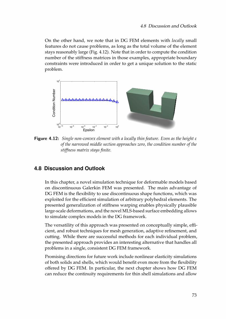
4.8 Discussion and Outlook
On the other hand, we note that in DG FEM elements with locally smallfeatures do not cause problems, as long as the total volume of the elementstays reasonably large (Fig. 4.12). Note that in order to compute the conditionnumber of the stiffness matrices in those examples, appropriate boundaryconstraints were introduced in order to get a unique solution to the staticproblem.
10−10
10−8
10−6
10−4
10−2
100
103
104
Epsilon
Con
ditio
n N
umbe
r
Figure 4.12: Single non-convex element with a locally thin feature. Even as the height ε
of the narrowed middle section approaches zero, the condition number of thestiffness matrix stays finite.
4.8 Discussion and Outlook
In this chapter, a novel simulation technique for deformable models basedon discontinuous Galerkin FEM was presented. The main advantage ofDG FEM is the flexibility to use discontinuous shape functions, which wasexploited for the efficient simulation of arbitrary polyhedral elements. Thepresented generalization of stiffness warping enables physically plausiblelarge-scale deformations, and the novel MLS-based surface embedding allowsto simulate complex models in the DG framework.
The versatility of this approach was presented on conceptually simple, effi-cient, and robust techniques for mesh generation, adaptive refinement, andcutting. While there are successful methods for each individual problem,the presented approach provides an interesting alternative that handles allproblems in a single, consistent DG FEM framework.
Promising directions for future work include nonlinear elasticity simulationsof both solids and shells, which would benefit even more from the flexibilityoffered by DG FEM. In particular, the next chapter shows how DG FEMcan reduce the continuity requirements for thin shell simulations and allow
73

Simulation of Deformable Solids
for the representation of small features and changing topology through themeans of enrichment textures.
74

C H A P T E R 5Enrichment Textures for Shells
Figure 5.1: Starting from a single shell element, the proposed method is able to capturecomplex deformations and topological changes by simply enriching the el-ement’s basis functions through texture maps (left). Fracturing a bunnytriangle mesh (right).
After having applied the discontinuous Galerkin finite element method to thesimulation of deformable solids as presented in the previous chapter, it onlyseems natural to think about how the simulation of thin objects, i.e. shells, canbenefit from the reduced continuity requirements offered by DG FEM. Withthat in mind, this chapter presents a method for simulating highly detailedcutting and fracturing of thin shells using low-resolution simulation meshes.
75

Enrichment Textures for Shells
Instead of refining or remeshing the underlying simulation domain to resolvecomplex cut paths, custom-designed basis functions are introduced thatenrich the approximation by accurately representing these detailed features.
The proposed approach generalizes the extended finite element method(XFEM) by storing the enrichment basis functions in enrichment textures,which allows for fracture and cutting discontinuities at a resolution muchfiner than the underlying mesh, similar to image textures for increased visualresolution. Furthermore, harmonic enrichment functions can handle multiple,intersecting, arbitrarily shaped, progressive cuts per element in a simple andunified framework.
By using an underlying shell simulation based on discontinuous GalerkinFEM, the restrictive requirement of C1 continuous shell basis functions isrelaxed and thus simpler, C0 continuous XFEM enrichment functions can beused. The DG shell method is further extended by a corotational formulationthat allows for the plausible simulation of large deformations while keepingthe computational cost low.
5.1 Overview
In order to simulate the deformation behavior of thin shells, it is not sufficientto formulate their mechanical behavior as described in Section 3.5. We alsoneed to provide an appropriate discretization, which due to the curvilinear co-ordinates and the involved differential equation (a fourth-order elliptic PDE)is non-trivial. Discontinuous Galerkin FEM provides a rather elegant way ofsolving this problem, by reducing the continuity requirements between ele-ments from C1 to C0. After presenting the DG FEM-based discretization andbasis functions for quad and triangle elements, corotation will be introducedsuch that large deformations can be simulated without the artifacts typicallyobserved for geometrically linear models.
The proposed method is then presented as a texture-based variant of theXFEM which is able to handle multiple cuts and partial cuts in a natural way,whereas traditional XFEM approaches need to handle those as special cases.The method is also able to cut through meshes consisting of several elementswhile keeping the support of the new basis functions local to the elementsintersected by the cut.
Next to shell simulation and topological changes, rendering is also an impor-tant aspect of the proposed method. The simulated features will be at thescale of a texture pixel rather than the size of a finite element, and simply
76

5.2 Discontinuous Galerkin FEM Thin Shells
tessellating the elements at a high resolution for rendering is not the best pos-sible approach. Instead, a renderer employing a geometry shader is proposedthat is able to resolve details at the texture level even for coarse tessellations.
5.2 Discontinuous Galerkin FEM Thin Shells
This section describes an implementation of the discontinuous Galerkin finiteelement method for thin shells presented by Noels and Radovitzky [2008].Building on the Kirchhoff-Love shell theory presented in Chapter 3, the DGweak form is reviewed and the assembly of the stiffness matrix is describedin detail. Extending on this previous work, a corotational extension to themethod is presented which allows for the simulation of large rotationaldeformations without the typical linearization artifacts of a linear shell model.
5.2.1 Shell Model
Eq. (5.1) shows again the weak form for the Kirchhoff-Love shell modelas it has already been presented in Section 3.5.2. This weak form couldbe discretized using a standard finite element approach [Hughes, 2000;Zienkiewicz and Taylor, 2000].
a(u,v) :=∫
Ωεαβ(v)Hαβγδ
n εγδ(u)dS
+∫
Ωραβ(v)Hαβγδ
m ργδ(u)dS (5.1)
However, a closer look at the weak form reveals that due to the second deriva-tives in the bending strain it represents a fourth order elliptic PDE, whichimplies that appropriate basis functions must lie in the Sobolev space H2(Ω),i.e. have square-integrable first and second order derivatives [Hughes, 2000].Unfortunately, constructing suitable shell functions on irregular meshes is arather complex task. A variety of approaches are in use, such as ignoring thecontinuity requirements or introducing additional variables, e.g. derivativesat edge mid-points [Zienkiewicz and Taylor, 2000]. Other approaches usenon-local interpolation schemes [Cirak et al., 2000].
A DG FEM approach for thin shells avoids the problem by only requiringbasis functions that are C0 across elements and enforcing C1 continuity ina weak sense. The formulation results in additional integrals over elementedges, which effectively introduce a deformation energy term which penal-izes discontinuities in the derivatives.
77

Enrichment Textures for Shells
In the case of DG FEM as described in Noels and Radovitzky [2008], the weakform becomes
aDG(u,v) := ∑K
aK(u,v) + ∑e
ae(u,v) (5.2)
for elements K and interior edges e (edges with neighboring elements on bothsides). aK corresponds to the weak form (3.36) evaluated on element K. ae isdefined on interior edges as follows:
ae(u,v) :=∫eJ∆t(v)K ·ϕ0,γν−δ Hm J∆t(u)K ·ϕ0,αν−β ηe dΓ
+∫
e
ραβ(v)Hmϕ0,γ
ν−δ · J∆t(u)K dΓ
+∫
eJ∆t(v)K ·
ραβ(u)Hmϕ0,γ
ν−δ dΓ. (5.3)
Considering an edge e, element K+ lies on the left-hand side of the directededge and element K− on the right-hand side. Quantities associated witheither element are superscripted with a − or +, respectively. J·K is the jumpoperator, defined in this context as
JvK := v+ − v−
and · the average operator, with its usual definition
v :=12(v+ + v−),
v :=12(v+ + v−)
for v ∈ IR3 and v ∈ IR. Note that the definitions of the jump and averageoperators used in the context of shells are different from the ones used inSection 3.1.2 for solid FEM. ηe is a penalty factor for edge e which dependson a global penalty parameter η and the local element size as follows:
ηe =η
he
where he is the characteristic size of the edge. The characteristic size iscomputed from the areas and circumferences of the two adjacent elementsusing
he = min( |A+||∂A+| ,
|A−||∂A−|
).
78

5.2 Discontinuous Galerkin FEM Thin Shells
In the above weak form, ∆t(u) is the change of the normal vector, which canbe computed as
∆t(u) =1j0
(ϕ0,1 × u,2 −ϕ0,2 × u,1
+ t0 u,1 · (t0 ×ϕ0,2)
− t0 u,2 · (t0 ×ϕ0,1)). (5.4)
ν− = (ν−1 ,ν−2 )T is the outer unit normal of K− represented in the conjugatebasis ϕ,α
0 , see (3.39).
Note that the first term in (5.3) penalizes the jump of the change of the normalvector t on the edge. In other words, J∆t(u)K is zero if the displacement field uchanges the normals t− and t+ on either side of the edge in the same way. Theother two terms in (5.3) are responsible for making the formulation consistentand symmetric, see Arnold et al. [2001].
5.2.2 Stiffness Matrix Assembly
This section describes in detail how the stiffness matrix K can be computedfrom element and edge contributions. Instead of following the formulation ofNoels and Radovitzky [2008], Voigt notation will be employed here in orderto avoid tensor notation and provide a more tangible implementation.
Basis Function Discretization. The undeformed shell surface is defined interms of basis functions Na : Ω→ IR as
ϕ0 = ∑a
NaXa0,
where Xa0 ∈ IR3 is the initial position of node a. It follows that the undeformed
surface basis vectors can be computed as
ϕ0,α = ∑a
Na,αXa
0,
by differentiating the basis functions Na with respect to ξ1 and ξ2. Similarly,the displacement field u is discretized as
u = ∑a
Naua
with nodal displacements ua. Representing the solution u as well as the testfunction v in terms of the basis functions Na results in a linear system
KU = F, with
Kij = aDG(I3Ni,I3N j)
Fi =∫
Ω f Ni, (5.5)
79

Enrichment Textures for Shells
which is solved for the degrees of freedom U = (u1T, . . . ,unT)T, given externalforces f.
Quad and Triangle Elements. As proposed in Noels and Radovitzky [2008],quadrangular elements with 8 nodes and bi-quadratic basis functions can beemployed. The basis functions are:
N1 = −14(−1 + ξ2)(−1 + ξ1)(ξ1 + ξ2 + 1)
N2 = −14(−1 + ξ2)(1 + ξ1)(ξ1 − ξ2 − 1)
N3 =14(1 + ξ2)(1 + ξ1)(ξ1 + ξ2 − 1)
N4 =14(1 + ξ2)(−1 + ξ1)(ξ1 − ξ2 + 1)
N5 =12(1− ξ1ξ1)(1− ξ2)
N6 =12(1− ξ2ξ2)(1 + ξ1)
N7 =12(1− ξ1ξ1)(1 + ξ2)
N8 =12(1− ξ2ξ2)(1− ξ1)
for element coordinates (ξ1,ξ2) with −1≤ ξ1,ξ2 ≤ 1.
When working with triangular 6-node elements, the following quadratic basisfunctions can be used
N1 = 1− 3ξ1 − 3ξ2 + 2ξ1ξ1 + 4ξ1ξ2 + 2ξ2ξ2
N2 = ξ1(2ξ1 − 1)N3 = ξ2(2ξ2 − 1)N4 = −4ξ1(−1 + ξ1 + ξ2)
N5 = 4ξ1ξ2
N6 = −4ξ2(−1 + ξ1 + ξ2)
where ξ1,ξ2 ≥ 0 and ξ1 + ξ2 ≤ 1. The node numbering for the two elementsis depicted in Fig. 5.2.
80

5.2 Discontinuous Galerkin FEM Thin Shells
Figure 5.2: Node numbering for the quadrangular (left) and triangular element (right).
Element Contributions. Similar to Cirak et al. [2000], the membrane straintwo-tensor can be represented in Voigt notation as
ε :=
ε11ε22
ε12 + ε21
.
The membrane strain in Voigt notation can then be computed as
ε = ∑a
Banua
where the 3× 3 matrix Ban is made up of three row vectors:
Ban :=
ban11
T
ban22
T
ban12
T + ban21
T
3×3
withba
nαβ :=ϕ0,αNa,β.
Similarly, the bending strain can be written in Voigt notation as
ρ :=
ρ11ρ22
2ρ12
,
which can be computed as
ρ = ∑a
Bamua
81

Enrichment Textures for Shells
where the 3× 3 matrix Bam is made up of three row vectors:
Ban :=
bam11
T
bam22
T
2bam12
T
3×3
with
bamαβ := ϕ0,αβ · t0
1j0
(Na
,1(ϕ0,2 × t0)− Na,2(ϕ0,1 × t0)
)+
1j0
(Na
,1(ϕ0,αβ ×ϕ0,2)− Na,2(ϕ0,αβ ×ϕ0,1)
)−Na
,αβt0. (5.6)
Next, we define the Voigt notation matrix H as
H :=
H1111 H1122 H1112
H2211 H2222 H2212
H1211 H1222 H1212
,
whereH is the constitutive tensor defined in (3.39). The constitutive tensorsfor membrane and bending stresses (in Voigt notation) can thus be defined as
Hn :=Eh
1− ν2 H
and
Hm :=Eh3
12(1− ν)2 H.
The assembly of an element’s membrane stiffness into the global stiffnessmatrix K can finally be written as
Kab+=∫
Ban
THnBbn dS , (5.7)
where Kab is the 3× 3 block of the stiffness matrix at position (a,b). Similarly,bending stiffness contributions are assembled using
Kab+=∫
Bam
THmBbm dS . (5.8)
During the element assembly, (5.7) and (5.8) are computed for all pairs ofelement basis functions a,b for all elements and added to the global stiffnessmatrix K as described above.
82
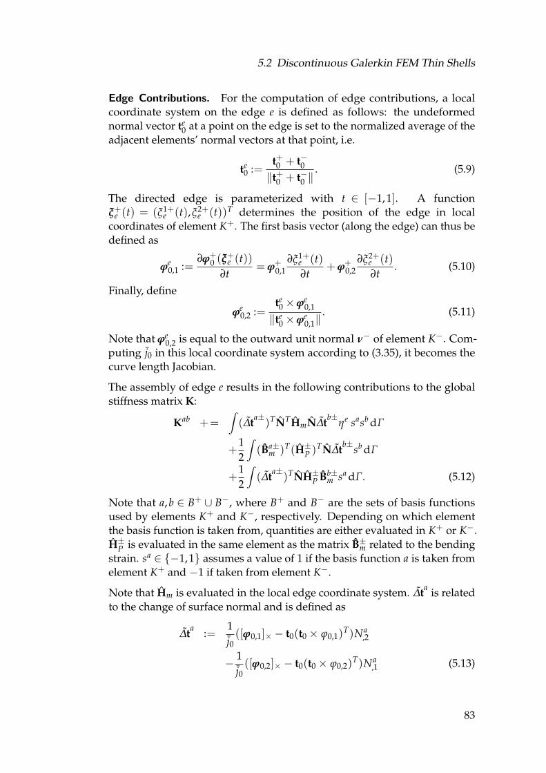
5.2 Discontinuous Galerkin FEM Thin Shells
Edge Contributions. For the computation of edge contributions, a localcoordinate system on the edge e is defined as follows: the undeformednormal vector te
0 at a point on the edge is set to the normalized average of theadjacent elements’ normal vectors at that point, i.e.
te0 :=
t+0 + t−0‖t+0 + t−0 ‖
. (5.9)
The directed edge is parameterized with t ∈ [−1,1]. A functionξ+e (t) = (ξ1+
e (t),ξ2+e (t))T determines the position of the edge in local
coordinates of element K+. The first basis vector (along the edge) can thus bedefined as
ϕe0,1 :=
∂ϕ+0 (ξ
+e (t))
∂t=ϕ+
0,1∂ξ1+
e (t)∂t
+ϕ+0,2
∂ξ2+e (t)∂t
. (5.10)
Finally, define
ϕe0,2 :=
te0 ×ϕe
0,1
‖te0 ×ϕe
0,1‖. (5.11)
Note that ϕe0,2 is equal to the outward unit normal ν− of element K−. Com-
puting j0 in this local coordinate system according to (3.35), it becomes thecurve length Jacobian.
The assembly of edge e results in the following contributions to the globalstiffness matrix K:
Kab +=∫(∆ta±
)TNTHmN∆tb±ηe sasb dΓ
+12
∫(Ba±
m )T(H±P )TN∆tb±sb dΓ
+12
∫(∆ta±
)TNH±P Bb±m sa dΓ. (5.12)
Note that a,b ∈ B+ ∪ B−, where B+ and B− are the sets of basis functionsused by elements K+ and K−, respectively. Depending on which elementthe basis function is taken from, quantities are either evaluated in K+ or K−.H±P is evaluated in the same element as the matrix B±m related to the bendingstrain. sa ∈ −1,1 assumes a value of 1 if the basis function a is taken fromelement K+ and −1 if taken from element K−.
Note that Hm is evaluated in the local edge coordinate system. ∆ta is relatedto the change of surface normal and is defined as
∆ta :=1j0([ϕ0,1]× − t0(t0 × ϕ0,1)
T)Na,2
− 1j0([ϕ0,2]× − t0(t0 × ϕ0,2)
T)Na,1 (5.13)
83

Enrichment Textures for Shells
with
[ϕ0,α]× :=
0 −ϕ30,α ϕ2
0,αϕ3
0,α 0 −ϕ10,α
−ϕ20,α ϕ1
0,α 0
. (5.14)
As the local edge coordinate system is orthogonal and ϕe0,2 = ν− and
‖ϕe0,2‖ = 1, it follows that ν−1 = 0 and ν−2 = 1. This fact can be used to
construct the matrix N as follows:
N :=
ϕ0,1Tν−1
ϕ0,2Tν−2
ϕ0,1Tν−2 +ϕ0,2
Tν−1
3×3
=
0T
ϕ0,2T
ϕ0,1T
3×3
. (5.15)
H±P represents the push-forward tensors and inverse transformation tensorscombined with the constitutive tensor and formulated as a 3× 3 matrix inVoigt notation:
H±P := (P±)TH±mP±p±, (5.16)
where
P± :=
P±1111 P±1122 P±1112P±2211 P±2222 P±2212
2P±1211 2P±1222 P±1212 + P±1221
(5.17)
withP±αβγδ := (ϕ,γ
0 ·ϕ±0,α)(ϕ,δ0 ·ϕ±0,β) (5.18)
and
p± :=
p±1111 p±1122 p±1112p±2211 p±2222 p±2212
2p±1211 2p±1222 p±1212 + p±1221
(5.19)
withp±αβγδ := (ϕ±,γ
0 ·ϕ0,α)(ϕ±,δ0 ·ϕ0,β). (5.20)
Assembly Algorithm. The three main equations for the assembly of theglobal stiffness matrix are (5.7), (5.8), and (5.12). Algorithm 5.1 shows themain assembly steps in pseudocode.
84

5.2 Discontinuous Galerkin FEM Thin Shells
1 Initialize global stiffness matrix K with zero2 for all elements K:3 for all a ∈ BK:4 for all b ∈ BK:5 Add membrane contribution (5.7) to Kab
6 Add bending contribution (5.8) to Kab
7 end8 end9 end
10 for all interior edges e:11 // Note: Elements adjacent to e are K+ and K−
12 for all a ∈ B+ ∪ B−:13 for all b ∈ B+ ∪ B−:14 Add edge contribution (5.12) to Kab
15 end16 end17 end
Algorithm 5.1: Summary of stiffness matrix assembly.
5.2.3 Dynamic Simulation
Given the stiffness matrix K, a dynamic simulation of time-varying forcesand displacements is governed by the equations
MU + DU + KU = F , (5.21)
which are solved by semi-implicit Euler integration. Note that instead oflumping element masses to nodes, the full mass matrix Mij =
∫Ω NiN j is
used, such that nodal basis functions and XFEM enrichment functions canlater be handled in a uniform way. Moreover, if an element will be split intomultiple parts, these will not only have the correct mass, but also the correctcenter of mass and moment of inertia.
5.2.4 Corotational DG FEM Shells
In its original formulation, the DG FEM treatment of Kirchhoff-Love shells ofNoels and Radovitzky [2008] is not suitable for most graphics applications,because it uses a geometrically linear strain, which results in artifacts in caseof large rotational deformations. We therefore propose a simple corotational
85

Enrichment Textures for Shells
extension that allows arbitrary rotational deformations while still keepingthe basic model linear in the displacements.
Following Muller and Gross [2004] and Thomaszewski et al. [2006], the strainis computed in an un-rotated coordinate frame and the resulting force rotatedback to its original orientation. As components of the same element candeform significantly differently as a shell element is bent, we apply the coro-tational formulation to each quadrature point i, similar to Mezger et al. [2008].For the assembly of element contributions into the global stiffness matrixK (Equations (5.7), (5.8)), numerical quadrature turns the integrals over theelements into per-quadrature point contributions Kabi
K :
Kab+= KabiK . (5.22)
Computing the strain in an un-rotated coordinate frame and rotating theresulting force back to its original orientation, the new contributions become
Kab += Ri KabiK RiT
, (5.23)
Fa += Ri KabiK (I−RiT
)Xb0. (5.24)
Note that a corrective term is added to the right-hand side F. Xb0 is the value
for basis function b that reproduces the undeformed configuration. For nodaldegrees of freedom, this corresponds to the undeformed position of node b.When combining this model with enrichment functions, non-nodal degreesof freedom will be introduced and appropriate values for Xb
0 must be definedfor them. This can be achieved by applying the same idea as described inSection 4.4.2 for the case of non-nodal basis functions for solid FEM. Ri is a3× 3 rotation matrix that describes the local rotation at quadrature point i. Itcan be computed by polar decomposition of the deformation gradient at thequadrature point [Thomaszewski et al., 2006].
The same steps are performed for the edge contributions Kabie , i.e., for the
penalty term that weakly enforces C1 continuity across edge e. This time,however, the rotation matrix is computed from the deformation gradient inthe edge coordinate frame.
Qualitative Evaluation. Fig. 5.3 shows an example of a nonlinear deforma-tion that would not be possible to simulate using a pure linear deformationmodel. The cylinder is fixed at both ends and slightly compressed, resultingin a typical buckling deformation. The mesh consists of 961 quad elementsand 2945 nodes, with a global stiffness matrix of size 8835× 8835.
86

5.3 XFEM Basics
Figure 5.3: Corotational DG FEM shells allow for the simulation of geometrically-nonlinear phenomena such as buckling (961 quad elements, 2945 nodes).
The DG FEM discretization of Kirchhoff-Love shells described so far allowsfor simple C0 basis functions and shows a plausible, geometrically nonlineardeformation behavior. However, to enable the simulation of highly detailedcuts or creases, as shown in Fig. 5.1, without excessively refining the underly-ing simulation mesh, we propose an XFEM approach that is described in thefollowing sections.
5.3 XFEM Basics
Introduced in Belytschko and Black [1999], the extended finite elementmethod (XFEM) builds up on the partition of unity concept [Melenk andBabuska, 1996]. The basic idea of XFEM consists in enriching an element bysplitting its basis functions along a desired discontinuity. This effectivelydoubles the element’s degrees of freedom and decouples the solutions oneither side of the discontinuity. In an elasticity simulation, this allows a singleelement to be cut or fractured into two independent parts.
Splitting the original basis functions along the discontinuity results in thecanonical basis, as shown for a 1D example in Fig. 5.4. We can define theenriched basis functions as the product of an original basis function Na(ξ)and a so-called enrichment function ψa(ξ). Arguably the simplest choice for theenrichment functions ψa(ξ) is the Heaviside function Hs(ξ), which assumesthe value of 0 on one side of the cut and 1 on the other side.
87

Enrichment Textures for Shells
(1! !1("))N1(")
(1! !2("))N2(")!2(")N2(")
!1(")N1(")N1(!)
N2(!)
!1 !2
!1 !2
!1 !2
!1 !2
!1 !2
!1 !2
Figure 5.4: The canonical basis: basis functions Na are split along the discontinuity tohandle both parts separately.
Note that the function space spanned by ψaNa and (1− ψa)Na is the same asthe one spanned by Na and ψaNa, and it does not depend on which side ofthe discontinuity we choose the Heaviside function to vanish. The splittingof the basis functions can therefore be realized by adding to the original basisfunctions Na the enrichment basis functions ψaNa with their correspondingdegrees of freedom aa. This yields the enriched displacement field
u(ξ) =n
∑a=1
Na(ξ)ua +n
∑a=1
ψa(ξ)Na(ξ)aa. (5.25)
XFEM therefore modifies the functional representation on a sub-element levelinstead of changing the topology of the element mesh. While traditionalmethods would have to divide existing elements into smaller elements inorder to resolve the geometry of the cut, XFEM achieves the same goalwithout complex remeshing.
Instead of the simple Heaviside function Hs(ξ), Zi and Belytschko [2003]proposed to use shifted enrichment functions
ψa(ξ) = Hg(ξ)− Hg(ξa), (5.26)
where Hg(ξ) = 2Hs(ξ) − 1 is the generalized Heaviside function (signumfunction), and ξa ∈Ω is the position of node a in parameter space. See Fig. 5.5for a 1D illustration. The shifted enrichment basis functions together with theoriginal basis functions span the same space as in the case of the unshiftedenrichment functions. They are thus equivalent to the canonical basis.
Defining the enrichment functions this way has two desirable properties.First, it keeps the enrichment local, in the sense that the enrichment basisfunctions are only supported within the cut element. Compare this to Fig. 5.4,where the enrichment basis functions extend to all elements incident to the
88

5.4 Enrichment Textures
!2(")N2(")
!1(")N1(")N1(!)
N2(!)!2(")
!1(")
=!
! =
!1 !2
!1 !2
!1
!1 !2
!1 !2
!1 !2
!2
Figure 5.5: Enrichment basis functions are obtained by multiplying the original basisfunctions by shifted Heaviside functions.
enriched node. This locality simplifies implementation and, according toJerabkova and Kuhlen [2009], also improves the stability of the simulation.
Second, shifting the enrichment functions recovers the Kronecker-delta prop-erty. The shifted enrichment function ψa vanishes at its associated node a, andas the nodal basis function Na vanishes at all nodes other than a, the enrich-ment basis functions ψaNa vanish at all nodal positions ξa. As a consequence,the displacement at each node a is fully defined by ua alone. This simplifiesthe implementation of Dirichlet boundary conditions, as the displacementof a node can be fixed to a specific value by constraining a single degree offreedom.
5.4 Enrichment Textures
Many researchers have considered various ways to generalize the Heavisidefunction Hg and the shifted enrichment functions ψa from 1D to 2D or 3D. Inmost approaches, discontinuities are represented by simple analytical func-tions, such as cutting planes for 3D elements and linear or quadratic cuttingpaths for 2D elements. This representation, however, is too restrictive forgraphics simulations, as it prevents us from having highly detailed, complexcuts through rather coarse elements of the simulation mesh.
To overcome this limitation, we represent the cut path as well as the gen-eralized Heaviside function as piecewise linear functions on a regular 2Dgrid, which will be referred to as enrichment texture in the following. Discon-tinuities will be represented as an edge path between texture pixels (texels).The texture values are interpreted as (samples of) the generalized Heavisidefunction H(ξ), and replaces Hg(ξ) in (5.26).
89

Enrichment Textures for Shells
Figure 5.6: A complete cut through a single element. The enrichment texture (128× 128)is a generalized Heaviside (left), taking on values of −1 (red) or +1 (blue) oneach side of the cut. A simulation of this enriched element is shown on theright.
Defining the enrichment function via a texture map has two important advan-tages. First, compared to analytic descriptions, it is better suited for modelingcomplex cutting paths, since the complexity of cuts is only limited by the tex-ture resolution. Second, when dealing with progressive cuts, partial cuts, ormultiple, intersecting cuts—required for cutting and fracturing simulations—it allows to handle the generation of the associated enrichment functions in astraightforward and uniform manner.
In this section we will focus on complete cuts, i.e., cuts that completely split anelement into two pieces, or into several pieces in case of multiple cuts. Themore complex problem of partial and progressive cuts will be discussed inSection 5.5.
5.4.1 Single Cut
In the simplest case, for a single, complete cut through an element, theenrichment texture stores a value of −1 or +1 for each texel, indicating whichside of the cut the texel lies on (see Fig. 5.6, left). This defines the HeavisideH(ξ), which we use to construct the enrichment functions ψa(ξ) as in (5.26).Multiplication with the original basis functions yields the enriched basisfunctions ψa(ξ)Na(ξ). Their partial derivatives can easily be computed byfinite differences on the regular texture grid. The functions and their gradientsare then integrated over the element to construct K and F, as shown in (5.5).To this end, the numerical integrator can simply sample the texture valuesat the quadrature points. These must be chosen densely enough so that allfeatures of the enrichment texture are captured. In the limit, this correspondsto one quadrature point per texel.
90

5.4 Enrichment Textures
Figure 5.7: Two complete, intersecting cuts through a single element, resulting in threeseparate connected components.
5.4.2 Multiple Cuts
When considering multiple cuts within a single element, a cut is called com-plete if it starts and ends either at the element’s boundary or at a junctionwith another cut. Multiple complete cuts therefore decompose the elementinto several connected components Ci.
The straightforward generalization of the canonical basis (see Fig. 5.4) is de-fined in terms of canonical Heaviside functions Hi
c(ξ), which are 1 within theircorresponding component Ci and 0 everywhere else. From these functionsone can construct the shifted enrichment functions and from there on proceedlike in the case of a single cut. Fig. 5.7 shows an example of two intersectingcomplete cuts, resulting in three physically independent surface components.
Note that thanks to our discrete texture representation the identificationof connected components can be done by a trivial flood fill algorithm. Incontrast, when representing cuts analytically, this task is more complex, suchthat often a hierarchical representation and classification of cuts has to beused.
5.4.3 Rendering
During a dynamic simulation, (4.11) is integrated in time, which in each timestep yields the displacement u(ξ) at the spatial resolution of the enrichmenttextures. For rendering the deformed and cut shell surface, we tessellate eachelement of the simulation mesh into a fine triangulation, in order to moreaccurately approximate the quadratic displacement function u(ξ) as well asthe high-resolution cuts. Note, however, that each element uses the samestatic triangulation, thereby minimizing storage and overhead.
91

Enrichment Textures for Shells
Figure 5.8: A cut triangle (left) is duplicated and rendered once for each side of the cut(right)
One option would be to generate a vertex for each texel, and have the tri-angulation implicitly defined by the regular texture grid, which would beconceptually similar to geometry images [Gu et al., 2002]. However, in orderto reduce the number of triangles, while still being able to resolve featuresat the texel level, we employ a geometry shader. This shader duplicatestriangles that have been cut: triangle vertices that lie on the opposite sideof the cut are linearly extrapolated, and the triangle is then rendered witha fragment shader that masks out texels on the opposite side of the cut (seeFig. 5.8). An edge of a triangle is considered to be cut if two criteria are
Figure 5.9: Visualization of the underlying triangle mesh (red wireframe). Note theduplication of triangles that are intersected by the cut.
met. First, the magnitude of the difference between the enrichment functionvalues at the edge’s vertices must exceed a certain threshold, and second,the sign of the enrichment function must be different at these two vertices.Fig. 5.6 shows an example of a complete cut through a single element, usingan enrichment texture of resolution 128× 128. Note that this approach limitsthe resolution of the cut to the texture resolution. Using texture filtering, the
92

5.4 Enrichment Textures
Figure 5.10: Comparison of rendering techniques. Removing triangles intersected by thecut (left), killing pixels close to the cut curve (middle), and duplicating cuttriangles while employing a geometry shader (right).
resulting aliasing artifacts can be mitigated to some degree. Fig. 5.9 visualizesthe underlying triangle mesh used to render an object consisting of a singleelement. To demonstrate the benefits of geometry shader based rendering,Fig. 5.10 compares simple triangle or pixel removal to the proposed approach,which is free of artifacts while keeping the width of the cut below the size ofone texture pixel.
Figure 5.11: Rendering each element independently highlights the discretization and C0
continuity (left), while a simple averaging of normals at element nodes canresult in a visually more pleasing representation (right).
Visual Surface Smoothness. As the initial surface as well as the deformedmesh are only required to be C0 continuous, a direct rendering of the physicalsimulation mesh can result in shading artifacts such as the creases in Fig. 5.11,left. If visual quality is more important than an accurate representation of the
93

Enrichment Textures for Shells
simulation geometry, vertex normals can be averaged between elements andinterpolated inside elements to get the shading of a C1 continuous surface asshown in Fig. 5.11, right.
5.5 Progressive Cutting
After showing the simplicity and flexibility of enrichment textures for completecuts, we now discuss the more interesting case of partial, progressive cuts. Inthis case, a cut does not (yet) fully separate the element into two independentcomponents.
For such configurations, works in the mechanics literature typically require toclassify a discontinuity into either a tip (partial cut), a complete cut, or a junction(intersecting cuts), and generate special enrichment functions depending onthe type of discontinuity. When furthermore allowing for multiple cuts withina single element, with cuts being either partial or complete, the combinatoricsof handling these different cases in a hierarchical representation inevitablyleads to rather complex implementations.
In this section we propose our harmonic enrichment approach, which is con-ceptually simpler, in that it uses only one kind of unified enrichment functionthat does not depend on the type of cut, and that generalizes to multiple,partial, progressive, and complete cuts in a natural and canonical manner. Weagain start with a single cut, then discuss multiple cuts within one element,and describe how to handle cuts that intersect multiple elements.
5.5.1 Single Cut
Since a partial cut does not fully split the element into two components,separation of material is only allowed along the curve covered by the cut sofar. However, as soon as a progressive cut has traversed the whole elementand hence became a complete cut, we want the parts on either side of thecut to be independent of each other, as shown in the previous section. Thistranslates into two conditions for the generalized Heaviside function:
• For a partial cut, the enrichment (and the Heaviside) should be dis-continuous along the cut but continuous everywhere else, allowingmaterial to separate at the cut only.
• If the progressive cut becomes a complete cut, the value of the enrich-ment function must be constant on either side of the cut, replicatingthe behavior of the Heaviside functions of the previous section.
94

5.5 Progressive Cutting
n
H = +1
H = !1
!H = 0
!H · n = 0
Figure 5.12: A partial cut in a single element: The corresponding Laplace problem(left), the resulting harmonic enrichment texture (center), and the elementbehavior in a simulation (right).
In mechanics, one of the classical crack tip functions is√
r sin(θ/2) [Be-lytschko and Black, 1999], where (θ,r) are polar coordinates centered atthe crack tip. This function takes on values of ±√r on either side of the crack.However, this function does not easily generalize to complex cut shapes andmultiple cuts within a single element. We therefore generalize the classicalenrichment function by observing that it is a harmonic function and definingharmonic enrichments as the solution to the Laplace equation
∆H(ξ) = 0, (5.27)
subject to suitable boundary conditions along the crack tip and the elementboundary. On the element boundary, we prescribe vanishing Neumannconstraints ∇H(ξ) · n(ξ) = 0 (see Fig. 5.12).
Along the crack, prescribing the Dirichlet conditions H(ξ) = ±√r recoversthe classical harmonic enrichment function
√r sin(θ/2) in the vicinity of the
crack tip as demonstrated in Fig. 5.13. In particular, since a harmonic recon-struction reproduces given boundary conditions (tautologically), it followsthat the influence of any other finitely-distant boundary can be ignored in asufficiently small neighborhood of the tip. As a simplification, we assumethat the
√r-decay is concentrated within the crack tip texel; thus, we pre-
scribe the Dirichlet conditions H(ξ) = ±1 on the texels incident to the cut.The simplified condition works well in our experiments; however, if adaptiverefinement of the enrichment texture is used, the
√r-decay should be explic-
itly considered, since the Dirichlet conditions ±1 are ill-posed in the smoothlimit.
Thanks to our texture representation, (5.27) can be discretized by a simplefinite difference scheme. As the cut corresponds to a series of connectededges between texels, the Dirichlet conditions set the texels incident to a cutedge to −1 or 1, respectively. The resulting sparse linear system has to be
95

Enrichment Textures for Shells
Figure 5.13: Comparison between the function√
r sin(θ/2) (left) and the finite differencesolution of ∆H(ξ) = 0 with Dirichlet boundary conditions H(ξ) = ±√ron the cut (right). The two solutions are identical up to discretization errors.
solved for the function values of H(ξ) at each texel, which we do using eithera multigrid solver or a sparse Cholesky factorization [Toledo et al., 2003].
As the solution of a Laplace equation, H(ξ) will be harmonic, i.e., continuousand smooth, everywhere except at the Dirichlet constraints, where it showsthe desired discontinuity. Hence, the first requirement is fulfilled. In thecase of a complete cut, the vanishing Neumann boundary conditions causeH(ξ) to replicate a Heaviside with constant ±1 on either side of the cut.Furthermore, as the cut approaches the element boundary, the enrichmentfunction converges to this Heaviside in a temporally smooth manner. As aconsequence, the second criterion is satisfied. The enrichment texture of thepartial cut in Fig. 5.12 would eventually converge to the one of the completecut shown in Fig. 5.6.
5.5.2 Multiple Cuts
With just a slight modification of the boundary constraints, the harmonicenrichment approach can be generalized from single cuts to multiple cutswithin an element. Consider n (partial or complete) cuts ci(ξ), 1≤ i ≤ n, inan element. We have to construct an enrichment function for each cut, i.e.,we have to find a generalized Heaviside Hi(ξ) for each cut ci(ξ). The tworequirements formulated for single cuts can be extended to multiple cuts asfollows:
• The enrichment function Hi(ξ) should be discontinuous across itscut ci(ξ), and continuous for unconstrained texels. Hi(ξ) might bediscontinuous across cj(ξ) for j 6= i.
• If all cuts are complete cuts, they partition the element into n + 1 sepa-rate components C1, . . . ,Cn+1. The original basis functions and their
96

5.5 Progressive Cutting
Figure 5.14: Multiple progressive cuts within an element: The harmonic enrichmenttextures Hi(ξ) for each of the cuts (left, center), and the resulting simulationbehavior (right).
n enriched versions should reproduce the behavior of the canonicalbasis (see Fig. 5.7), i.e., they should span the same function space.
We extend the definition of harmonic enrichment functions for multiple cutsas follows: each enrichment function Hi(ξ) is again defined as the solution of
∆Hi(ξ) = 0. (5.28)
As in the single cut case, the discontinuity across its corresponding cut ci(ξ)is enforced through Dirichlet conditions of ±1. However, now we enforcevanishing Neumann conditions not only on the element boundary, but alsoon all other cuts cj(ξ), j 6= i, i.e.
∇Hi(ξ) · n(ξ) = 0, (5.29)
where n is the normal of either the domain boundary or another cut cj(ξ)respectively. Note that there might be components with Neumann conditionsonly. These components are independent of the cut ci under consideration,and we therefore explicitly set the function values in these regions to zero. Theresulting Heaviside functions Hi(ξ) again trivially satisfy the first conditionby construction. A simple proof showing that the second condition is alsofulfilled is given in Appendix A.2. See Fig. 5.14 for an example of two partialcuts, which would eventually converge to the situation depicted in Fig. 5.7.
Harmonic enrichment textures therefore allow us to handle both single andmultiple cuts, as well as partial, progressive, and complete cuts in a simple,unified, and canonical manner. In contrast to existing work, we do not requirecuts to be classified into crack tips, joints, or complete cuts. Neither do weneed a complex hierarchical representation to keep track of multiple cuts andthe resulting connected components.
97

Enrichment Textures for Shells
5.5.3 Multiple Elements
So far, we described how to handle single or multiple, partial or complete cutswithin a single element. For realistic simulations, however, a simulation meshof more than one element is of course required. In this section we extendour enrichment approach to multiple elements partitioning the simulationdomain Ω. A 2D illustration of a multi-element mesh with two complete cutsc1, c2 and one partial cut c3 is shown in Fig. 5.15.
!
!3
!2
!1
c1
c2c3
Figure 5.15: Three cuts define nodes to be enriched (dots) and associated domains Ωion which the Hi are defined. Nodes in overlapping domains are enrichedmultiple times.
In order to model the discontinuities caused by a cut, all elements intersectedby this cut are enriched. This is achieved by enriching the nodal basis func-tions Na(ξ) of each of the element’s vertices a, resulting in ψa(ξ)Na(ξ). Thisexpression requires the enrichment function ψa, and therefore the HeavisideH (see (5.26)), to be defined on the whole support of Na, which in our case isjust the set of elements incident to vertex a. The (overlapping) colored regionsΩi in Fig. 5.15 highlight the elements that are enriched due to the respectivecuts ci, the dots represent the vertices to be enriched.
The main difference to the single element case is that the enrichment functionsof neighboring elements have to be C0 continuous across their shared edge,in order to guarantee the enrichment basis functions ψaNa, and thus theenriched displacement u (see (5.25)), to be C0, as required by our DG FEMformulation.
For complete cuts, such as c1 and c2 in Fig. 5.15, we can use the simple en-richment functions shown in Figs. 5.6 and 5.7 for the intersected elements,
98

5.6 Results
and constant enrichments of +1 or −1 for their neighboring elements. Theresulting enrichment functions will be C0 across mesh edges by construction.
The handling of partial cuts, such as c3 in Fig. 5.15, is slightly more involved.For the element containing the cut tip a harmonic enrichment is computed bysolving (5.27) or (5.28), as discussed in Section 5.5.2. The vanishing Neumannboundary conditions for this system can, however, not guarantee C0 conti-nuity to its neighboring elements (as Dirichlet boundary constraints coulddo).
In order to ensure continuity, we additionally have to take the incident ele-ments into account and solve the Laplace equation on this extended one-ringneighborhood (3× 3 region around the tip of c3 in Fig. 5.15). On the bound-ary edges of this region we prescribe the values of neighboring enrichmentfunctions, if they exist, as C0 Dirichlet constraints, or vanishing Neumannconditions otherwise. As the neighboring enrichment function values werecomputed in previous simulation steps, this construction is free of cycles.
In Fig. 5.15 we would therefore compute the enrichment function(s) H3 forthe nine elements around the cut tip by a single Laplace system, prescribing±1 Dirichlet constraints along c3, vanishing Neumann constraints along c1,C0 Dirichlet constraints on the boundary to the blue elements, and vanish-ing Neumann constraints on the other boundaries. In this 3× 3 region theenrichment function H1 for cut c1 also has to be computed through this sys-tem, by exchanging the roles of c1 and c3. With this slight modification ofthe domain and the constraints of the Laplace systems (5.27), (5.28), we areable to generalize the harmonic enrichment textures from single elements toarbitrary simulation meshes, including quad and triangle meshes throughthe definition of appropriate texel neighborhoods at the element boundaries.
Note that our DG FEM formulation considerably simplifies this generalizationas it only requires C0 continuity on element edges. On the other hand, con-forming thin shell discretizations using C1 basis functions [Cirak et al., 2000;Thomaszewski et al., 2006] would require C1 continuous enrichment func-tions, which cannot be computed through simple Laplace systems.
5.6 Results
We demonstrate our enrichment method on a variety of examples, includingsingle elements, more complex element meshes, single progressive cuts, cutsconsisting of multiple enrichments, and multiple cuts per element. Thesimulation meshes used consist of either 8-node bi-quadratic quadrilateral
99

Enrichment Textures for Shells
elements or 6-node quadratic triangular elements. All discontinuities wereprescribed as polylines and then rasterized to texel edges.
Complex Cut Lines. Our method allows us to represent discontinuities on afine sub-element level without the need to remesh. Fracture lines are a specialinstance of such discontinuity lines and are usually computed using localstrain or stress measurements to predict their evolution. We do not directlysimulate a complex fracturing model but generate the highly-detailed cutboundaries procedurally. Our approach is able to resolve the shells’ reactionto the fracture discontinuity at the sub-element level, as shown in Fig. 5.16.
Figure 5.16: A single textured quad element being fractured (left), and the underlyingdiscontinuous enrichment function (right).
Fig. 5.1, right, shows the same model applied to a non-trivial mesh with trian-gular quadratic elements. Note that the elements are shaded independentlyof each other in order to show the coarse resolution of the simulation mesh.To avoid these shading discontinuities, normals can be averaged at nodesand interpolated over the elements as described in Section 5.4.3.
Small Features. The presented approach allows us to simulate small scaledetails down to the resolution of the texture. In Fig. 5.17, left, a circular cutis applied to a planar shell mesh consisting of four quads. The method canrobustly handle the situation where the connection between the “hangingchad” and the rest of the element is only a few texels wide. Without requiringany special handling, the basis functions resulting from the harmonic enrich-ments introduce a specific additional mode of deformation, leading to theexpected result. Fig. 5.17, right, shows an example of a highly-detailed cutline demonstrating the capability to resolve small features.
100

5.6 Results
Figure 5.17: Simulation of a chad failing to completely separate from a punchcard (left).Highly detailed cut on a tissue (right).
Multiple Cuts. As described in Section 5.5.2, our method is also applicableto the case of multiple cuts per element. Fig. 5.1, left, shows a single quadelement that has been enriched 18 times, replicating a “paper accordion”. Inthis example, the boundary conditions on the cuts are not purely±1 on eitherside of the cuts, but instead are blended to zero towards both ends of eachcut to get an enrichment that better captures the desired deformation.
Figure 5.18: A quad element is cut by a helical line, using a single enrichment (left) andsix cut segments (right). The insets show the enrichment functions used.
For long progressive cuts with complex trajectories, a single enrichment willnot provide sufficient additional degrees of freedom to allow for the desireddeformation. Such cases can be handled consistently by tracking the lengthor integral angle of the cut and by initiating a new cut once a predefinedthreshold is exceeded. While this criterion is mathematically not rigorous, itworks very well in practice, and we employed it for our experiments.
This results in a series of connected cuts that together make up the desireddiscontinuity and add the required local degrees of freedom. Fig. 5.18 showsan example of a spiral cut enriched by a single enrichment texture (left),lacking the desired deformation, and the same curve divided into 6 cuts
101

Enrichment Textures for Shells
(right), resulting in a more plausible simulation. Applying the same principleto a less trivial mesh, a slinky is cut out of a cylinder in Fig. 5.19, left. Fig. 5.19,right, additionally shows an example of intersecting cuts. Note that once acut crosses another cut, it becomes a complete cut that ends at the point ofintersection and a new cut is started.
Figure 5.19: A cylinder represented by four quad elements is cut into a slinky, deformsunder gravity and uncoils (left). Simulation of intersecting cuts in a singleelement (right).
Material Textures. As an alternative application of textures besides cutting,we can define material properties at the texel level. In the case of Kirchhoff-Love shells, properties that can be modulated by such a material textureinclude the material’s Young’s modulus, Poisson’s ratio, as well as the localthickness of the shell. During the integration of an element’s stiffness matrix,the material texture is evaluated at the quadrature points. Fig. 5.20 shows anexample of a single shell element with locally reduced thickness, causing it toweaken and exhibit a stronger deformation under gravity. In this example,122 quadrature points were used to integrate the element’s stiffness matrix.
Figure 5.20: The thickness of a shell element (left) is modulated by a thickness textureand deforms accordingly (right).
102

5.6 Results
Figure 5.21: A C0 continuous enrichment texture with discontinuous first derivatives(left) allows adding a crease to an element (right).
Creases. So far, we have only considered enrichment textures with disconti-nuities, allowing for cutting and separating shells into multiple independentcomponents. However, we note that the concept of enrichment textures ismore general. In particular, it can also be used to model sharp creases, atwhich the shell is free to bend. Creases can be modeled by keeping the en-richment textures C0 continuous, but introducing discontinuities in the firstderivatives. Fig. 5.21, left, shows an example of an enrichment texture for acurved crease line. The enrichment function is computed as the geodesic dis-tance from the crease using a fast marching method [Sethian, 1999]. Applyingthis enrichment texture to a shell element allows the element to bend aroundthe crease, resulting in interesting states of minimal energy when externalforces are applied (see Fig. 5.21, right).
Model #Els. #Nodes #Enr. Tex. tenr tasm tsolChad 4 21 1 256 1433 16 3Spiral 1 1 8 1 256 274 1.8 0.1Spiral 6 1 8 6 256 1701 38 0.7Accordion 1 8 18 256 4785 313 8Bunny 552 1106 1 32 283 452 917Slinky 4 20 12 128 5207 513 22
Table 5.1: Comparison of timings for the computation of the enrichment functions (tenr),assembly of the global stiffness matrix (tasm), and solving the resulting linearsystem (tsol). Timings are in milliseconds and were taken on an Intel Core2Duo 2.4 GHz.
Timings. Table 5.1 shows the computation times per simulation step for arepresentative selection of examples. The times for computing the enrich-ments are peak values, while the assembly and solve times were averaged
103

Enrichment Textures for Shells
over the whole simulation. For solving the Laplace problem during thecomputation of the enrichment functions, we employ a sparse Choleskysolver [Toledo et al., 2003].
Comparison to Discrete Shells. For typical meshes the cost of cutting andenrichment is only a small percentage of the total simulation time, e.g., 7% forthe Bunny example. This percentage vanishes as mesh resolution increases,since the cost of dynamics increases while the texture area intersected by thecut decreases.
Focusing on the bulk of computational cost—simulating dynamics aftercutting—Table 5.2 compares our method to Discrete Shells [Grinspun et al.,2003] in terms of computational effort. We use the number of non-zero entriesin the stiffness matrix (NNZ) as a measure of complexity for solving the linearsystem during time integration. For Discrete Shells, the mesh resolutionswere chosen to match the NNZs of our enriched simulations.
For the Discrete Shells simulations, the mesh resolution might be sufficientto simulate the elastic behavior, but it is not enough to resolve the cuts insufficient detail, especially for highly detailed cuts. By contrast, our enrich-ment uses the same number of additional DOFs, whether the cut is highlyjagged or straight. The comparison shows that our method excels in settingscharacterized by a higher ratio of cut to deformation complexity.
Mesh (Method) #Els. #Nodes #DOFs #NNZBunny (our method) 552 1106 3318 243954Bunny (Discrete Shells) 4200 2102 6306 245934Spiral (our method) 1 8 168 28224Spiral (Discrete Shells) 385 274 822 32058Chad (our method) 1 8 48 2304Chad (Discrete Shells) 72 62 186 7254
Table 5.2: Comparison of our method to Discrete Shells with a comparable computationalbudget (non-zero stiffness matrix entries).
Limitations. The previous examples show that our method is able to rep-resent complex cut lines and small features in single elements and elementmeshes, and that multiple cuts per element can be handled consistently.
However, we note that our current implementation of the method lacks aproper projection step. When the basis functions change due to enrichment,we simply apply the previous solution to the new basis. In most situations
104

5.7 Discussion and Outlook
the introduced error is unnoticeable, since the enrichments change graduallyover time. However, in some scenarios it leads to obvious “popping” artifacts,e.g., in the multiply enriched spiral of Fig. 5.18, right. These artifacts may beeliminated by projecting the displacements and velocities onto the new basis,as proposed, e.g., in Rethore et al. [2005].
5.7 Discussion and Outlook
We presented a novel method for handling highly detailed discontinuityfeatures such as cutting or fracture lines using a versatile, texture-basedbasis enrichment approach. The method spends new degrees of freedomin an economical manner and supports a uniform and general treatment ofmultiple progressive or complete discontinuities. While the proposed methodfocuses on introducing material discontinuities, we hope that the presentedway of combining texture concepts with physical simulations opens excitingnew areas for future work.
A promising direction for future work is to generalize the modeling of creases,building on the preliminary results presented in this work. We would alsolike to explore the synergies of textures representing both geometric andphysical material properties. For example, a displacement texture map couldrepresent both the physical rest state of a shell as well as allow for highsurface detail while still only requiring a coarse simulation mesh.
We further note that most of the steps in the simulation pipeline are veryamenable to parallelization, making them ideal candidates for computationon the GPU. In particular, the computation of the enrichment functionscan be performed efficiently using a multigrid solver, whose pre- and post-smoothing steps can be interpreted as simple texture filtering operations [Bolzet al., 2003]. The corotated stiffness matrix integration could be computed onthe GPU, since it parallelizes trivially, leading to a highly accurate integrationat the texel level. At the rendering stage, the deformed geometry could easilybe constructed on the GPU as well, by computing the displacement field fromthe enrichment textures and the solution to the dynamic simulation.
The presented corotational extension of the linear discontinuous Galerkinshell method of Noels and Radovitzky [2008] allows for the simulation ofnonlinear phenomena while still being efficient to compute. The use of DGFEM in this context not only provides a practical solution to the C1 continu-ity problem of thin shells, it also simplifies the computation of enrichmenttextures for multi-element cuts.
105

Enrichment Textures for Shells
So far, we have only applied DG FEM to linear problems (with corotation).The next chapter will present an application where the method is used tosolve non-linear problems in the context of image warping.
106

C H A P T E R 6Non-Linear Image Warping
a b c d e
Figure 6.1: Our unifying representation of image warping supports efficient adaptivemeshing, high order basis functions, and more. a) Original image, b) auto-matic saliency map, c) aspect ratio change by uniform scaling, d) retargetingusing uniform grid (6767 vertices), e) similar quality results using an adap-tive mesh (1325 vertices).
After having applied the DG FEM to the simulation of deformable solids andshells in the previous two chapters, we now show that the method can alsobe used to solve content-aware image warping problems in a single unifyingframework that encompasses a wide range of image and video editing tasks.In this field, even standard FEM is not widely used yet. Instead, existingapproaches define error terms over mesh edges or vertex finite differences.As will be shown, these can be expressed as a special case of the proposedFEM model.
107

Non-Linear Image Warping
We exploit the full generality of FEMs, gaining important advantages, suchas: arbitrary mesh connectivity in the image domain, a well defined, continu-ous problem formulation, and well behaved convergence properties. Theseadvantages are then used to demonstrate support for adaptive meshing,allowing for efficient temporally stable solutions, and robust and simpleconstraint substitution, allowing for fine level control over warping results.An FEM representation also naturally supports higher order basis functions,allowing for smoother warps even with a small number of elements.
Through the use of DG FEM, per-element basis functions of varying degreeand complex mesh connectivity with hanging nodes can be used, which fur-ther increases the space of possibilities and simplifies the problem setup. Thecontinuous problem formulation allows us to clearly analyze existing imagewarping error functions, and propose improved ones. The utility of the pro-posed method is demonstrated by showing examples in adaptive, temporallyconsistent content-aware video resizing and camera stabilization applications,and by comparing our results to previous state of the art methods.
6.1 Overview
In order to formulate image warping problems in a generic 2D FEM frame-work, we first need to understand their underlying continuum equations. Itturns out that for most of the energy terms and constraints that have pre-viously been used in the image warping literature, this is a pretty straightforward task. While the FEM is more general in theory, we limit ourselvesto warp energies that are defined in terms of an energy density that onlydepends on position as well as first spatial derivatives of the warp. Thisallows us to directly apply the non-linear FEM theory presented in Section 3.2and Section 3.3.
Formulating all warp energies as energy density functions will allow us tocompare and classify them, and in some cases even to simplify them bycoming up with new energies that have similar properties but a simplermathematical formulation. The benefits of DG FEM will become obviousonce we look at the actual discretization of the problem: one of the generaladvantages of FEM over finite difference methods is that FEM allows foradaptivity, so degrees of freedom can be spent where they are most needed,i.e. in areas where the solution changes rapidly. With DG FEM, one caneven go one step further as the method naturally supports hanging nodes,which makes adaptive meshing (h-refinement) almost trivial. It additionallyallows for easily combining elements with different polynomial degrees
108

6.2 FEM for Image Warping
(p-refinement) to further adapt the distribution of DOFs to the underlyingproblem.
Finally, FEM image warping is demonstrated in the domain of media retar-geting, where the aspect ratio of images or videos is modified such that theshape of important content is preserved, as well as video stabilization, wherea smooth reconstruction of hand-held shaky videos is computed. For videoretargeting, adaptive solutions will be shown that allow us to solve a wholesequence of frames at once; a task that previously would be either compu-tationally intractable, or have only low resolution control due to excessivesubsampling.
6.2 FEM for Image Warping
In order to derive an FEM for image warping, we begin by formulatingthe general image warping problem in the continuous case, and then inSection 6.3 we will discuss application specific decisions. While previousapproaches first set up the discretization using finite differences, regularlyspaced grids, or triangle meshes, computing ad-hoc energy functions fromthe resulting primitives (vertices, edges), a continuous formulation allows usto study and compare the properties of various image warping energies inde-pendently of their discretization. We then perform the actual discretizationby means of finite elements as a second, independent step, where we are pre-sented with a multitude of choices, allowing us for example to trade accuracy(how well the continuous solution is approximated) for performance.
6.2.1 Continuous Warping
Consider the rectangular domain Ω = [0,1]× [0, h] ⊂ IR2 of an undeformedimage. The warping function ϕ : Ω→ IR2 maps a point X = (X1, X2)
T ∈ Ω
to a warped point x = (x1, x2)T = (ϕ1(X1, X2), ϕ2(X1, X2))
T = ϕ(X) (seeFigure 6.2). Following the notation introduced in Section 3.3, let the 2-dimensional deformation gradient be defined as the 2× 2 matrix F(X) withentries:
Fij(X) =∂ϕi
∂Xj
∣∣∣∣X
In order to define the cost of performing a certain warp ϕ, we again make useof a function Ψ that computes the deformation energy density (per undeformed
109

Non-Linear Image Warping
area in 2D) at any point X ∈Ω. The total deformation energy of a warp ϕ canthen be computed as:
E[ϕ] =∫
ΩΨ(F(X))
The optimal warp is the one that minimizes E, and respects a number ofproblem-specific boundary constraints defined in Section 6.3.
Ω
𝑥1 𝑋1
𝑋2 𝑥2
𝐗 𝐱
𝛗
Figure 6.2: Continuous mapping from the undeformed domain to the warped image usinga simple nonuniform scale warp.
6.2.2 FEM Discretization
Now that we have defined the continuous image warping problem, wediscretize the problem using the FEM in order to numerically compute theoptimal warp.
Basis Functions. As a first step, we proceed as described in Section 3.3.2and discretize the warping function ϕ into a linear combination of n basisfunctions Ni : Ω→ IR with associated weights xi = (xi
1, xi2)
T ∈ IR2:
ϕ(X) ≈n
∑i=1
xiNi(X) (6.1)
Once the shapes of the individual basis functions have been defined, thewarping function ϕ is fully determined through the values xi. The continuousproblem of finding a function ϕ reduces to finding the vectors x1, . . . ,xn thatminimize E. The xi are thus the degrees of freedom (DOF) of our optimizationproblem.
110

6.2 FEM for Image Warping
Mesh Representation. The domain Ω is represented as a mesh consistingof m elements K1, . . . ,Km, and q nodes at positions X1, . . . ,Xq. Computing thederivative of Eq. (6.1) with respect to X gives us F as a linear combination ofxi. The energy E can now be formulated as a sum over element integrals:
E =m
∑k=1
∫Kk
Ψ
(n
∑i=1
xi∂Ni
∂X
∣∣∣∣ T
X
)dX (6.2)
The per-element integrals can be approximated using a numerical quadraturerule. For implementation details, we refer to Hughes [2000]. What makes thiscomputation efficient is the fact that basis functions Ni are local: inside anyelement Kk, only a constant number of basis functions can be non-zero, andthe sum over i can be reduced to a sum over those basis functions.
If we treat each pixel of an image as an element with a single constantbasis function, and introduce some additional terms to handle the resultingdiscontinuities between elements, we are in fact able to recover the standardfinite difference scheme that is used in existing image warping methods.
Numerical Minimization. For general Ψ(F), Eq. (6.2) is a non-linear equa-tion in xi, and we can minimize it using a Newton method [Nocedal andWright, 2000]. The Newton-Raphson method presented in Section 3.3.2worked well in our experiments. For this, we need the first and secondderivatives of E with respect to the xi, which we compute using either a codegeneration tool or automatic differentiation (AD). The second derivatives ofE result in a sparse, symmetric matrix H, which may not be positive-definite.Merging all the vector DOFs xi into one big vector d of length 2n and denotingthe first derivative of E by f, a single Newton step computes the increment∆d of d by solving the linear system
H∆d = −f (6.3)
using a direct solver for sparse positive definite systems [Schenk et al., 2001].
The pseudocode function ComputeE defined in Algorithm 6.1 computes theenergy E for given DOF values d. It calls ComputePsi to evaluate the energydensity Ψ for the given deformation gradient F. ComputeBFunDeriv computesthe derivative of a basis function at a given position. EC computes the energyof constraint C for the given DOF values.
111

Non-Linear Image Warping
1 ComputeE( d = (x1T, . . . ,xnT)T )2 E← 03 for each element Kk:4 for each quadrature point qj with weight wj of Kk:5 F← 06 for each basis function Ni of Kk:7 b← ComputeBFunDeriv(i, qj)8 F+= xi bT
9 end10 E+= ComputePsi(F) wj
11 end12 end
13 for each soft constraint C:14 E+= EC(d)15 end
16 return E17 end
Algorithm 6.1: Computation of the energy E.
6.3 Application Specifics
We have now defined image warping in the continuous sense and presentedthe generic framework of non-linear FEM. At this point we still have to makea choice about the basis functions Ni, the mesh connectivity K1, . . . ,Km, andthe energy density function Ψ. Now we discuss how we may want to pickthese for different image warping applications.
6.3.1 Deformation Energy Densities
One of the main application-specific questions is what kind of energy densityfunctions Ψ we want. We look at several different possible formulations,showing how our continuous formulation allows us to not only reproduceexisting warping energies used in earlier work, but also more clearly under-stand their limitations and design new constraints. We start by defining someimportant quantities from continuum mechanics [Bonet and Wood, 1997].
Most of the commonly used deformation energy densities for image warp-ing can be computed from a combination of quantities derived from the
112

6.3 Application Specifics
deformation gradient F(X). F itself can also be useful here, as it tells us howan infinitesimal line segment dX at position X gets deformed under ϕ. Thedeformed line segment dx can be computed as dx = FdX. Another usefulquantity is the Jacobian determinant J defined as:
J(X) = det(F(X)) (6.4)
The Jacobian determinant tells us how an infinitesimal area changes underthe deformation ϕ. We will make frequent use of the right Cauchy-Greentensor C defined as
C(X) = F(X)TF(X), (6.5)
which is invariant under rotation and thus any energy density that can beexpressed in terms of C will inherit its rotational invariance. Analyzing theeigenvalues λ1,λ2 of C(X), one can see that
√λ1 and
√λ2 are the principal
stretches of the deformation at X, i.e. the minimum and maximum values forthe stretch that can be achieved for any direction dX at position X [Sander etal., 2001].
Translational Invariance. As shown in Shamir and Sorkine [2009], one sim-ple energy density for image warping is the one that penalizes all deforma-tions except for translations
ΨF = ‖F− I‖2F, (6.6)
where I denotes the 2× 2 identity matrix and ‖·‖F denotes the Frobeniusnorm of a matrix (see Appendix B). ΨF is only quadratic in derivatives of ϕ,so when using this energy density, the minimum of a discretized deformationenergy E can by found in a single Newton step.
Scaling Invariance. For energies that result in more complex optimiza-tion problems, existing methods usually employ alternating iterative meth-ods [Shamir and Sorkine, 2009] that solve a linear least-squares problemwhile fixing the values of some quantities, like a uniform scale. On the otherhand, once we have found the corresponding continuous formulation of suchenergies, our FEM framework can then solve the resulting non-linear problemin a consistent way.
For example, Wang et al. [2008] and Laffont et al. [2010] penalize all trans-formations other than translation and uniform scaling. The correspondingcontinuous energy density can be written as:
ΨF = ||F− J12 I||2 (6.7)
113

Non-Linear Image Warping
Rotation Invariance. The right Cauchy-Green tensor C is equal to the iden-tity matrix for pure rotations, a fact we can use to find an energy densitypenalizing only translations and rotations [Wang et al., 2010]:
ΨC = ||C− I||2 (6.8)
Similarity Invariance. The distortion energy used in Zhang et al. [2009] alsoallows for scaling invariance, permitting elements to undergo a similaritytransform (quadratic in derivatives of ϕ). Its corresponding energy density is:
ΨS = tr(C)− 2J (6.9)
Figure 6.3: Comparison between the energy densities ΨC − 2 (green) and ΨS (red) fornon-uniform scaling with F =
(s 00 1).
While this allows for an efficient minimization of E in a single Newton step,this energy density has the drawback of tolerating inversions. As can beseen in Figure 6.3, ΨS assumes a finite value when the stretch s in directionX1 becomes negative. Our continuous formulation allows us to design analternative energy density ΨC that possesses the same invariance to scalingand rotation but increases to infinity as s approaches zero, thus preventinginversions:
ΨC = J−2||C||2 (6.10)
For practical considerations, it helps to leave this energy density undefinedfor J ≤ 0. This will prevent the Newton solver from ever taking a step thatwould invert an element, and instead results in the line search finding anincrement ∆d such that J remains positive at every quadrature point.
114

6.3 Application Specifics
Input & sal. Linear ΨF (T) ΨF (T, S) ΨC (T, R) ΨS (T, S, R) ΨC (T, S, R)
Figure 6.4: Comparison between different deformation energy density functions in animage retargeting application, with indicated invariance to translation (T),scaling (S), and rotation (R). Note the self-intersection in the second rightimage, which is eliminated by our proposed energy density ΨC.
One can show that ||C||2 = λ21 + λ2
2 and J2 = λ1λ2, from which we derive analternative representation of ΨC,
ΨC =λ2
1 + λ22
λ1λ2=
(λ1 − λ2)2
λ1λ2+ κ, (6.11)
where the constant κ = 2 does not depend on the warp and can thus bedropped from the energy density function. The last equations show that ΨCessentially measures the difference between the squares of the minimum andmaximum stretches
√λ1,√
λ2 of the deformation, divided by J to achieveinvariance to uniform scaling. It thus measures the ‘non-uniformity’ of thescaling, while being invariant to rotations and uniform scaling.
Line Bending. One common energy term that comes up in image warp-ing methods prevents bending of mesh edges [Wang et al., 2008]. In theundeformed state, these edges are exactly horizontal and vertical, meaningthat this constraint is anisotropic and only works to preserve horizontal andvertical lines in an image. A straightforward application of the deformationgradient to the line segments (dS, 0)T and (0,dS)T leads to the correspondingcontinuous energy density:
Ψ = C11 − F11√
C11 + C22 − F22√
C22 (6.12)
However, the same effect can be achieved by using the simpler
ΨL = F212 + F2
21, (6.13)
which effectively penalizes shearing deformations along the main axes. This isidentical to the ‘edge preservation’ constraint used in Krahenbuhl et al. [2009]and Wolf et al. [2007].
115

Non-Linear Image Warping
𝑎 𝑎
0
1 1 𝑋
𝑋𝑌
𝑋2
𝑌
𝑌2
Figure 6.5: Values of nodal basis function Ni in a triangle mesh (left) and a quad mesh(middle), and the six basis functions used for quadratic DG FEM elements(right).
Visual Saliency. A key component of many content-aware image warpingmethods is the inclusion of a visual saliency term. The higher the saliency ofa region, the better should it be ‘preserved’ in the warp. This can be easilyincluded in our formulation by multiplying the energy density by somespatially varying saliency function γ(X) > 0. For the results shown here,γ was computed using a recent state-of-the art method from Goferman etal. [2010].
We have presented a small selection of possible energy density terms in orderto demonstrate how such terms can be created, and what their effects are onimage warping applications. By representing energy densities in these generalterms, not only can we replicate existing solutions, but it also allows us todiscover new insights and provide improvements, such as ΨC, an energy thatallows similarity transforms while explicitly preventing inversions. Figure 6.4shows a collection of these energy densities used in an image retargetingapplication.
6.3.2 Basis Functions
In standard FEM, nodal DOFs are used, meaning that q = n and every DOFis associated with a node: the DOF xi directly represents the solution of thewarp at node i. This implies that for all i, the basis function Ni(X) assumes avalue of 1 at position Xi, and a value of 0 at all Xj with i 6= j. The natural choicefor basis functions for simple triangle and quad elements are the linear andbi-linear basis functions, respectively (see Figure 6.5). These basis functionsare used in most prior work, and restrict the methods to averaging content(such as image saliency) within elements. With the FEM, saliency informationis sampled at multiple quadrature points during the numerical integrationallowing more accurate deformation penalties.
116

6.3 Application Specifics
Figure 6.6: Retargeted image using 81 bilinear quads (left, 100 DOFs) vs. 9 cubic quads(middle, 90 DOFs) and the corresponding deformed mesh (right). Usinghigher order basis functions yields smoother results.
DG FEM. In discontinuous Galerkin FEM, each element is endowed withits own set of basis functions. Using nodal basis functions is still possiblein this context, but in contrast to standard FEM, each element using thecorresponding node will have its own DOF associated with that node. Thebig advantage of the method is that we are no longer restricted to nodalbasis function but we can use simple polynomials of arbitrary order, wherethe order of polynomials can be chosen independently for each element.For example, the basis functions 1, X1, X2, X2
1, X1X2, X22 allow an element to
approximate the solution quadratically (see Figure 6.5).
To restore the coupling between elements, some additional terms are nec-essary. There are several possible ways to achieve this using DG FEM, butit all comes down to how the bi-valued function ϕ is replaced by the so-called numerical flux ϕ on the edges between elements. We proceed exactly asdescribed in Section 3.2, using the numerical flux of Bassi and Rebay [1997].
For rendering elements with higher-order basis functions, we triangulateeach element using a fine triangulation and compute the new positions of thetriangle mesh vertices by evaluating ϕ inside the element. A penalty term isused to reduce the size of gaps between elements. These gaps are then smallenough (sub-pixel size) to not cause artifacts in the warp and for renderingwe additionally average the values of ϕ on edges between elements.
Figure 6.6 shows where higher order basis functions are beneficial. Linearelements can result in visible ‘kinks’ between elements because they cannotrepresent bending, while higher order basis functions result in smoothertransitions between elements.
117

Non-Linear Image Warping
Figure 6.7: Error-based adaptivity for DG FEM with linear, quadratic and cubic quadelements (approx. 1024 DOFs each)
6.3.3 Mesh Construction
We take advantage of well behaved convergence properties of the FEM (seeFigure 6.8), and our mesh-independent formulation of the continuous imagewarping problem to propose an adaptive mesh. We can refine the mesh inimportant areas to achieve a high quality solution while drastically reducingthe number of DOFs, allowing for temporally stable solutions with a tractableproblem size.
While we can use any mesh subdivision technique, we demonstrate a coupleof simple choices. One method that we use is computed from a Delaunaytriangulation [Shewchuk, 1996] of a point set distributed according to variancein saliency, which allows for increased resolution in areas that are most likelyto contain changes in local deformation.
When using DG elements, we gain some additional freedom for mesh con-struction. In particular, the edges of neighboring elements are not requiredto coincide, creating hanging nodes. This allows for the use of adaptivequadtree meshes. Additionally, DG FEM gives rise to an error-based refine-ment scheme. As the amount of discontinuities between elements is a directindicator of the local error of the solution, refining the elements with thehighest discontinuities will reduce the global error in a greedy fashion andalso reduce the amount of visible gaps, resulting in a mesh where the functionvalues on edges can safely be averaged for rendering. See Figure 6.7 for anexample.
6.3.4 Additional Constraints
Boundary Conditions. Depending on the particular application, wemay want to constrain all nodes on the boundary of Ω such that(xa
1, xa2)
T = (Xa1s1, Xa
2s2)T if the image is stretched by (s1, s2)
T, or allow
118

6.3 Application Specifics
1E‐9
1E‐8
1E‐7
1E‐6
1E‐5
1E‐4
1E‐3
1E‐2
1E‐3 1E‐2 1E‐1 1E+0
error
h
Figure 6.8: Error∫
Ω ||ϕ− ϕ||2 with respect to a reference solution ϕ for meshes withdifferent element size h, showing nice convergence properties. The image onthe right shows the solution for h = 1/8. ΨF was used as the energy density.
nodes to slide on the boundary, by constraining xa1 = Xa
1s1 for nodes withXa
1 = 0 or Xa1 = 1 and similarly for the X2 direction. These constraints can
be implemented as hard constraints by modifying the first and secondderivatives of E such that the constrained DOFs do not get modified during aNewton step.
Weak Point Constraints. For certain applications like camera stabiliza-tion [Liu et al., 2009] and stereoscopic disparity editing [Lang et al., 2010],we want a weakly enforced point constraint such that PW gets warped to aspecific position pW . Such constraints can be realized by adding an energyterm for each point constraint:
EW = γW
12||ϕ(PW)− pW ||2 (6.14)
Line Constraints. We can also impose line constraints on the warp to weaklyenforce straight lines to remain straight after the warp [Krahenbuhl et al.,2009], or to warp initially curved lines to straight ones [Carroll et al., 2009].Similar to previous approaches, we parameterize the best-fitting straight lineas sin(α)x1 + cos(α)x2 + b = 0. For each line constraint, an additional energyterm is added to our minimization problem, computed as the integral of thesquared distance between the warped curve and the closest point on thefitted straight line, weighted by a penalty γL:
EL =12
γL
∫ l
0(sin(α)p1(s) + cos(α)p2(s) + b)2ds (6.15)
119

Non-Linear Image Warping
Figure 6.9: Frames from retargeted video sequences. Showing the input frame, linearscaling, FEM warping, and the corresponding mesh.
We use per-element quadrature to evaluate this integral. These kind ofconstraints can be incorporated seamlessly into our method: the two newunknowns α and b parameterizing the fitted straight line simply become twonew scalar DOFs of our non-linear problem, and no further special treatmentis necessary.
Temporal Stability. When dealing with video sequences, consistency ofoutput over time is important. Working with per-frame warps, we can for-mulate this as weak constraints that force an object to deform in a similarway in each frame of the video. Given a position Xt in frame t and a corre-sponding position Xt+1 in frame t + 1, our constraint tries to minimize thedifference between the deformation gradients at these points, taking intoaccount object and camera rotation and scaling represented as the matrix Gt.The corresponding energy is:
ET = γT
12||GtFt(Xt)G−1
t − Ft+1(Xt+1)||2 (6.16)
120

6.4 Results
a b c
Figure 6.10: Comparison of temporal stability in video retargeting on a syntheticdataset. Cropped results showing: a) original image, b) two frames fromKrahenbuhl et al. [2009] (note the difference in shape of the object), and c)same two frames from our method.
This constraint couples the otherwise independent DOFs of frames t andt + 1. One possibility of retrieving the correspondence between Xt and Xt+1
and the transformation Gt is by using SIFT feature tracking.
6.4 Results
While the presented framework itself is more general and could be appliedto any warping problem, this section shows results for two image warpingapplications.
Video Retargeting. For different video retargeting applications, we canchoose various energy density functions. Simple ones like ΨF, ΨS are attrac-tive for performance reasons, because the solution can be found in a singleNewton step. For difficult cases and extreme aspect ratio changes, one thatprevents inversions such as ΨC is preferable. To solve over a whole sequenceof frames and still keep the problem at a tractable size, we use an adaptivetriangle mesh and standard FEM. See Figure 6.9 for examples.
We compare the temporal stability of our method to prior work byKrahenbuhl et al. [2009] in Figure 6.10.
Video Stabilization. Warping-based video stabilization methods [Liu etal., 2009] consist of tracking feature points over time, reconstructing theirpositions and the camera in 3D space, then reprojecting feature points into anew, stabilized camera path. The input to the image warp consists of a set ofweighted feature points with source and (reprojected) target positions, whichguide the warp as weak point constraints. Additionally, we select an energy
121

Non-Linear Image Warping
Figure 6.11: Our image warping method applied to camera stabilization. Input framewith detected features (left), stabilized frame with FEM mesh (right).
Figure 6.12: Line constraints controlling the appearance of objects in a modified perspec-tive. Input image with triangle mesh and constrained lines shown in red(left), warp without line constraints (middle), warp with line constraints(right).
density function that is invariant to rotation. Good choices are ΨC or ΨC, butΨS works well, too, because the amount of deformation is typically low forthis particular application. There is no direct influence between the warpscomputed for individual frames, so each frame can be warped independentlyand a regular mesh of size 64× 36 as used in Liu et al. [2009] provides a goodquality-vs-performance trade-off. See Figure 6.11 for examples.
Other Applications. There are other methods that while we have not fullyreimplemented them, follow from our earlier definitions. For example, Fig-ure 6.12 shows an example of user line constraints, which are used as a meansof creating artistic perspective corrections [Carroll et al., 2010]. In addition, byusing our weak point constraints on stereo correspondences, we can performstereoscopic disparity editing [Lang et al., 2010].
122

6.5 Discussion and Outlook
Timing. We show the timing of our method on several examples in Table 6.1.These results were generated on an Intel Core i7 3.2 GHz, with a single-threaded application.
Example Ψ #Els #Frames #Newton tpre tHf tsolve
Fig. 6.1, right ΨC 2612 1 7 60 2 19Fig. 6.9, wakeboarder ΨF 111124 234 1 27820 600 6311Fig. 6.9, wind surfer ΨF 54249 117 1 14634 273 2537Fig. 6.11 ΨC 1152 1 2 31 2 4
Table 6.1: Problem complexity and timings (in ms) for precomputation (including meshgeneration), computation of H, f, and solving the linear system
Limitations. One limitation to our FEM approach is that it can be morecomplex to implement than traditional methods, especially when using DGFEM. However, this is a one-time cost, and when completed, the frameworkis very flexible, making application to novel problems and domains a muchsimpler task than before.
Our method supports high order basis functions. However, there is a trade-offwith using these. While fewer elements are needed, there are more degreesof freedom per element. In addition, it also results in denser systems to solve.However, the decisions to what kind of basis function should be used can bemade by the specific applications, weighting advantages and disadvantagesof either.
In addition, with non-linear image warping problems, it is difficult to proveconvergence guarantees, and it is possible with extreme warps the optimiza-tion method may result in a local minimum that does not correspond toour desired solution. However, this is true with existing methods as well,and we did not observe this behavior in any of our examples. Furthermore,our representation allows for easy substitution of energy densities, meshformulation, and minimization methods, potentially making dealing withlocal minima a simpler problem to resolve.
6.5 Discussion and Outlook
In conclusion, we have presented a novel, general representation for imagewarping that unifies a wide range of existing solutions. Our approach pro-vides a well defined continuous mathematical formulation that has multiple
123

Non-Linear Image Warping
real-world advantages. For one, a mathematical basis allows for energy densi-ties to be clearly defined and analyzed, allowing for improved understandingand design. Our representation is independent of the mesh formulation,which allows for simple extensions for adaptive meshing and temporallystable solutions, and naturally permits higher order basis functions, whichallow smoother warps using a small number of elements. However, probablymost significantly, there is a wide range of literature and ongoing researchabout FEM techniques in the mechanics and geometry communities, andby phrasing the image warping problem in the same context, both areas ofresearch have the potential to benefit tremendously from their combinedresearch efforts.
At this point, we have only scratched the surface of what the FEM could beused for in the context of image editing applications. Further insight intoFEM and related methods could provide additional capabilities, such as usingXFEM for discontinuous warping methods. Our representation is also notrestricted to 2D elements, and one extension could be a mesh subdivisionwith 3D elements, such as a video cube oct-tree, that may provide stabilityfor temporal solutions. In addition, it is possible that energies with higherorder derivatives could be useful, e.g. for the spherical distortion application.
124

C H A P T E R 7Conclusion
This chapter discusses the main contributions of this thesis and looks atpotential future work.
7.1 Discussion
While focusing on the simulation of deformable solids and shells as well asimage warping, this thesis has shown that DG FEM approaches can com-pete with, or even outperform, traditional finite element methods in certaincomputer graphics applications. Overall, the benefits of DG FEM did notso much turn out to be of a quantitative nature (resulting in significantlybetter performance or faster convergence). Instead, the application of DGFEM lead to elegant solutions to existing problems, with one method solvingseveral issues at once, and in some cases it turned out to allow for resultsthat simply were not possible using existing methods. As a by-product, someof the contributions made by this thesis go beyond, or are even orthogonalto DG FEM and may find broader applications in other areas of computergraphics. This includes for example the exact integration of polynomialsover polyhedra, the concept of enrichment textures, or the analysis of imagewarping energy terms using tools from material science.
Chapter 4 presented a simulation technique for deformable solids basedon DG FEM. The discontinuous shape functions of DG FEM allowed thesimulation of arbitrary polyhedral elements using simple polynomial basisfunctions that can even be integrated exactly (up to machine precision) within
125

Conclusion
elements. A corotational adaption of DG FEM allowed for large rotationaldeformations while still using a fast linear deformation model for elasticity.Smooth deformation fields computed using MLS allow for the embedding ofhigh resolution surface geometry, even in the presence of element separationand overlaps due to the discontinuous nature of DG FEM. As a consequence,mesh modifications become easier to handle in the proposed DG FEM frame-work, which was demonstrated through the simulation of progressive cutting,adaptive element refinement, and a novel mesh generation approach that canrepresent complex surface geometries with only a few elements.
In Chapter 5, a corotational extension of a linear DG FEM shell model waspresented, which allows for the simulation of nonlinear phenomena suchas buckling while still being efficient to compute. Making use of the factthat DG FEM can deal with C0 continuous basis functions for shell models,a novel basis function enrichment method has been presented that allowsfor the simulation of very detailed cut and fracture curves even on coarsesimulation meshes. These discontinuities are represented in what we termedenrichment textures, discretely sampled functions that modify the existingset of basis functions. In this framework, incomplete cuts, progressive cuts,the interplay of multiple cuts, and cuts extending over several elements canbe handled in a uniform way by solving a Laplace problem with suitableboundary conditions. To visualize the results of such simulations in real time,a novel rendering method based on a geometry shader was presented.
Applying DG FEM to image warping, Chapter 6 presented a unified frame-work that encompasses a wide range of existing warping approaches. Thanksto the underlying continuous mathematical formulation, existing energydensities can be analyzed and improved, and new energies with desirableproperties designed from scratch. The main benefit of FEM over alternativeapproaches is that it supports irregular domains and flexible meshing. Thisfeature allows for adaptively sampling the warp to concentrate DOFs wherethey are most needed, which in turn reduces the total number of DOFs with-out significantly reducing the accuracy of the computed solution. Thanksto this, large problems where a solve is computed over several images, suchas temporally stable video retargeting, now become tractable. The use ofDG FEM allowed for even more aggressive adaptivity by choosing higherpolynomial degrees in elements where the solution is expected to show amore non-linear behavior. Also, DG FEM simplifies the process of generatingan adaptive mesh. While a simple quad-tree would not be a valid mesh forCG FEM due to hanging nodes, DG FEM can handle such meshes withoutproblems. This is computationally easier and less error prone than computinga “nice” adaptive triangulation of the image domain.
126

7.2 Future Work
7.2 Future Work
While the focus of this work was on applying discontinuous Galerkin meth-ods to elliptic problems, there are certainly other problem types with relevantapplications in graphics, fluid simulations being the prime example. Infact, these were amongst the first problems to which DG FEM had been ap-plied [Bassi and Rebay, 1997]. Fluid simulation applications could potentiallybenefit from the adaptive meshing, or dynamic meshing to handle changingboundary conditions in the simulation of fluid-solid interaction.
Another exciting aspect of DG FEM that has not been considered in this thesisis space-time adaptivity [Altmann et al., 2010]. Just as a spatial element meshis allowed to have hanging nodes in DG FEM, a spatio-temporal mesh cancombine elements that have shorter or longer lifespans, and the interactionbetween these elements is automatically handled by the numerical fluxes.In computer graphics, this concept could again be applied to the simulationof deformable objects or fluids, resulting in dynamic simulations that au-tomatically, and locally, adapt the size of their time steps to reduce overallsimulation times.
Deformable Solids. One obvious extension to the proposed method forthe simulation of deformable solids is its application to nonlinear materialmodels. The same benefits as for linear models can be expected here, andadditionally, DG FEM may offer ways to handle degenerate cases moregracefully. Elements under stress that would otherwise get inverted could tosome degree be compensated by the discontinuities between elements.
Collision handling has been limited to simple point-plane collisions, butfull collision handling including self-collisions would be required for manypractical applications. For linear elements, existing techniques for collisiondetection and handling on triangle meshes could be used. Higher orderelements will bend under deformation and thus need special handling forcollision detection on polynomial surfaces, which could be an interestingtopic for future research.
One further advantage of DG FEM that has not been exploited in this workis that it can quite easily be parallelized [Devine et al., 1993; Noels andRadovitzky, 2006]. The simulation mesh can be partitioned in advance, andcomputations on each part can be performed in parallel. The only way theseparts exchange information is through the numerical fluxes on the elementboundaries. It could be interesting to investigate how well this idea wouldextend to the simulation of deformable objects, especially as today’s multi
127

Conclusion
core machines and highly parallel GPUs are indicators for how computingresources will have to be used in the future.
Enrichment Textures for Shells. The representation of material disconti-nuities as texture maps can be seen as a first example that may motivateinvestigation in other areas where physical simulations can be enhanced bythe use of texture concepts. Some preliminary work in this direction hasalready been shown: thickness textures can define shells with locally varyingthicknesses. Borrowing from existing uses of textures, e.g. displacementmaps or bump maps used in rendering, one could also think of displacingthe undeformed surface of a shell according to a texture map. This approachwould allow for coarse shell elements with highly detailed surfaces.
As shown in Section 5.6, enrichment textures can also be used to representcreases. The problem of how to compute physically motivated enrichmentfunctions for creases, especially in the presence of other discontinuities, re-mains an open problem. Solving the Laplace problem is still a bottleneckwhen simulating progressive cuts in our implementation. However, thiscomputation as well as the rest of the simulation pipeline can be expected tobe parallelizable on the GPU without too much effort, which would open upthe door to real-time applications such as games.
Image Warping. By formulating the warping problem in an FEM context,the doors are wide open to take advantage of the vast body of FEM researchand to apply the latest research results to problems in image warping. Ourwork has really only scratched the surface of what is possible. One interestingapproach could be to apply the XFEM and in particular enrichment texturesto image warping, to allow for discontinuous warps with details at the pixellevel, while still simulating only coarse elements. Additionally to what hasbeen shown in this work, there may be other concepts from the mechanicsand geometry communities that could be applied to image warping. Afterall, there is a close relationship between how real physical materials deformand how one expects a warped image to behave.
In this work, the warp energies and constraints have been limited to onlyinvolve first spatial derivatives. For some applications such as sphericaldistortion correction, the involved energies use higher order derivatives andit would be interesting to extend our method to support those as well. Finally,starting from the temporally stable video retargeting approach with adaptiveper-frame meshes, one obvious direction for future work is to look at the
128

7.2 Future Work
video cube as a three-dimensional domain and use 3D elements in an oct-tree fashion to approximate the solution. Elements would thus also have atemporal dimension, and the mesh would be adaptive in space as well astime, further reducing the total number of degrees of freedom of the problem.
129

Conclusion
130

A P P E N D I X ADerivations and Proofs
This appendix shows the details of derivations and proofs mentioned inearlier chapters.
A.1 Derivation of IP DG Weak Form for Linear Elasticity
This section shows the detailed derivation of the DG weak form for theinterior penalty method (see Equation (4.3)).
Notation. The average operator · has the same meaning for scalars andtensors as in Chapter 4. Additionally to the J·K jump operator mappingvectors to matrices and vice versa, the jump operator J·Ks maps vectors toscalars and vice versa as follows:
JuKs :=u− · n− + u+ · n+,JsKs :=s−n− + s+n+.
Identities. We will be making use of the following identities, where v andn represent vectors and σ represents a matrix.
Jv · σKs = JvK : σ+ v · JσK, (A.1)
J·K = JJ·KK = 0, (A.2)
131

Derivations and Proofs
J·Ks = JJ·KKs = 0, (A.3)
J·K = J·K, (A.4)
· = ·, (A.5)
v · σ · n = (v⊗ n) : σ. (A.6)
A.1.1 Strong Form
Recall the strong form of the linear elasticity PDE, formulated as two firstorder PDEs:
σ = C : ε(u), (A.7)∇ · σ = −f. (A.8)
A.1.2 Local Weak Form
The domain Ω gets triangulated into elements K. The space of the functionsu and σ is restricted to polynomials on each element (P(K) and Σ(K), respec-tively). Multiplying Equations (A.7) and (A.8) by a tensor test function τ andand a vector test function v, respectively, and integrating over element K,gives ∫
Kτ : σ =
∫K
τ : C : ε(u), ∀τ ∈ Σ(K), (A.9)∫K∇ · σ · v = −
∫K
f · v, ∀v ∈ P(K). (A.10)
Noting the identity∫Ω
σ : ε(v) = −∫
Ω∇ · σ · v +
∫∂Ω
v · σ · n (A.11)
and applying this to the right-hand side of (A.9) and the left-hand side of(A.10) results in the local weak form of element K:∫
Kτ : σ = −
∫K∇ · (τ : C) · u +
∫∂K
u · (τ : C) · n, ∀τ ∈ Σ(K), (A.12)∫K
σ : ε(v) =∫
Kf · v +
∫∂K
v · σ · n, ∀v ∈ P(K). (A.13)
132

A.1 Derivation of IP DG Weak Form for Linear Elasticity
Fluxes. Introducing fluxes u and σ in (A.12) and (A.13) to define the bi-valued functions u and σ on ∂K gives∫
Kτ : σ = −
∫K∇ · (τ : C) · u +
∫∂K
u · (τ : C) · n, ∀τ ∈ Σ(K), (A.14)∫K
σ : ε(v) =∫
Kf · v +
∫∂K
v · σ · n, ∀v ∈ P(K). (A.15)
A.1.3 Global Weak Form
Generalizing the flux definition from Arnold et al. [2000] to tensors, we getthe following fluxes for the IP method:
u = u,σ = C : ε(u) − η f JuK.
Sum Over Elements (First Part of Weak Form). The following equationsare to hold ∀τ and ∀v. Summing (A.14) over all elements K and inserting thepreviously defined IP flux we get
∑K
∫K
τ : σ = −∑K
∫K∇ · (τ : C) · u + ∑
e∈εh
∫eJu · (τ : C)Ks.
Note that εh denotes the set of all element edges, including ∂Ω and all edgesbetween elements. Using (A.11) this becomes
∑K
∫K
τ : σ = ∑K
∫K(τ : C) : ε(u)−∑
K
∫∂K
u · (τ : C) · n
+ ∑e∈εh
∫eJu · (τ : C)Ks
= ∑K
∫K(τ : C) : ε(u) + ∑
e∈εh
∫eJ(u − u) · (τ : C)Ks.
Using (A.1) we get
∑K
∫K
τ : σ = ∑K
∫K(τ : C) : ε(u)
+ ∑e∈εh
∫eJu − uK : τ : C+ u − u · Jτ : CK.
Because of (A.5) it holds that u − u = 0 and the above can be simplifiedto
∑K
∫K
τ : σ = ∑K
∫K(τ : C) : ε(u) + ∑
e∈εh
∫eJu − uK : τ : C.
133

Derivations and Proofs
Using (A.3) we finally get
∑K
∫K
τ : σ = ∑K
∫K(τ : C) : ε(u)− ∑
e∈εh
∫eJuK : τ : C. (A.16)
Sum Over Elements (Second Part of Weak Form). Summing (A.15) overall elements K and inserting the previously defined flux we get
∑K
∫K
σ : ε(v) =∫
Ωf · v + ∑
K
∫∂K
v · (C : ε(u) − η f JuK) · n
=∫
Ωf · v + ∑
e∈εh
∫eJv · (C : ε(u) − η f JuKKs.
Using (A.1) we get
∑K
∫K
σ : ε(v) =∫
Ωf · v+
∑e∈εh
∫eJvK : C : ε(u) − η f JuK+ v · JC : ε(u) − η f JuKK.
Because of (A.2) and (A.3), it holds that JC : ε(u) − η f JuKK = 0, so aftersome reordering the above simplifies to
∑K
∫K
σ : ε(v) (A.17)
− ∑e∈εh
∫eJvK : C : ε(u)+ ∑
e∈εh
∫eη f JvK : JuK =
∫Ω
f · v.
Eliminating σ. Using τ = ε(v) in (A.16) gives
∑K
∫K
ε(v) : σ = ∑K
∫K
ε(v) : C : ε(u)− ∑e∈εh
∫eJuK : C : ε(v). (A.18)
We can now insert (A.18) into (A.17) to get the primal formulation whichdoes not depend on σ:
∑K
∫K
ε(v) : C : ε(u) (A.19)
− ∑e∈εh
∫e
[JvK : C : ε(u)+ JuK : C : ε(v) − η f JvK : JuK
]=∫
Ωf · v.
Note that the left-hand side of the above equation is symmetric in u and v.
134

A.2 Basis for Multiple Complete Cuts
A.2 Basis for Multiple Complete Cuts
In this section we show for n complete cuts ci, the harmonic enrichmentfunctions Hi, obtained by solving ∆Hi = 0 for each cut ci as described inSection 5.5.2, span the same function space as the canonical basis for theresulting n + 1 components.
The canonical Heaviside functions Hic are the enrichment functions that produce
the canonical basis. Hic is 1 in component Ci and 0 otherwise. The canonical
enrichment basis of n + 1 components is
Cn+1 = H1c , . . . , Hn+1
c .
For an un-cut element, which is described by its original basis functions Na
only, the canonical enrichment function is H1c ≡ 1. In order to proof that our
enrichment basis functions span the same space as the canonical basis, itsuffices to show that the space
Hn+1 = 1, H1, . . . , Hn ,
spanned by our harmonic enrichment functions Hi and the constant 1 func-tion corresponding to the original basis, is equivalent to the space spannedby the canonical enrichment functions Cn+1.
This can be shown by induction as follows: For the case with n = 1 com-ponents, the constant 1 function is the only enrichment function and allenrichments are trivially equivalent to the canonical basis.
In the inductive step we assume that for n components the set of enrichmentfunctionsHn spans the same space as the canonical enrichments Cn. Hence,Hn spans an n-dimensional space and the Hi are linearly independent.
Then a new cut cn splits a component, say Cn, into two parts Cn and Cn+1, thusleading to n + 1 components. The spaceHn+1 is computed by solving (5.28)for each H1, . . . , Hn. Note that the i-th functions ofHn andHn+1 (1≤ i≤ n− 1)are not equal, since the new cut imposes additional Neumann conditionsat cn for (5.28). However, the additional Neumann conditions cannot turnthe new functions H1, . . . , Hn linearly dependent. Consequently,Hn+1 \ Hn
spans an n-dimensional subspace. The additional new function Hn is linearlyindependent ofHn+1 \ Hn, since it is the only Heaviside that can control bothsides of the new cut cn (i.e., Cn and Cn+1) independently. This means thatHn+1 must be a complete basis for an (n + 1)-dimensional space and thus isequivalent to the canonical basis Cn+1.
135

Derivations and Proofs
136

A P P E N D I X BNotation and Theorems
This appendix covers commonly used notation and summarizes relevanttheorems.
B.1 Mathematical Notation
Matrix Entries. The ‘bracket operator’ with subscript ij returns the entry atthe i-th row and j-th column of matrix A:
(A)ij := Aij
for
A =
A11 A12 · · ·A21 A22 · · ·· · · · · · . . .
.
Kronecker Delta. The Kronecker delta is defined as
δij :=
1 if i = j,0 otherwise.
137
Notation and Theorems
Scalar Product. The scalar product “·” between two n-dimensional vectorsa = (a1, . . . , an)T and b = (b1, . . . ,bn)T is defined as
a · b :=n
∑i=1
aibi.
Outer Product. The outer product “⊗” between two n-dimensional vectorsa and b is defined as
a⊗ b := abT.
Colon Operator. The colon operator “ :” denotes the tensor product be-tween two matrices A and B or between a matrix A and a 4-tensor C as
A :B := ∑ij
AijBij,
A :C := ∑ij
AijCijkl,
C :A := ∑kl
CijklAkl.
Matrix Operators. The trace of an n× n matrix A is defined as
tr(A) :=n
∑i=1
(A)ii
Norms. The 2-norm of a vector v is defined as
‖v‖ :=√
v · v.
The Frobenius norm of a matrix A is defined as
‖A‖F :=√
A :A.
Derivative Operators. A coma denotes partial differentiation. For a scalarfunction u : IRn→ IR:
u,i :=∂u∂xi
.
The gradient of a scalar function u : IRn→ IR is defined as
∇u := (∂u/∂x1, . . . ,∂u/∂xn)T.
138

B.2 Theorems
The divergence of a vector function v : IRn → IRn with v = (v1, . . . ,vn)T isdefined as
∇ · v = div v :=n
∑i=1
∂vi
∂xi
The Laplacian of a scalar function u : IRn→ IR is defined as
∆u =∇2u :=∇ · ∇u =n
∑i=1
∂2u∂x2
i.
DG Average and Jump. Unless specified otherwise, the average operator· and the jump operator J·K for scalar-valued functions u and vector-valuedfunctions v are defined as
u :=12(u− + u+
), JuK := u−n− + u+n+, (B.1)
v :=12(v− + v+
), JvK := v− · n− + v+ · n+
where n− =−n+ is the outward normal vector of the element on the ‘−’-sideof the edge.
B.2 Theorems
Integration by Parts (Higher Dimensions). For an open bounded subset Ω
of IRn with a piecewise smooth boundary ∂Ω and continuously differentiablefunctions u and v, it holds that∫
Ω
∂u∂xi
v =∫
∂Ωuvni −
∫Ω
u∂v∂xi
(B.2)
where ni is the i-th component of the outward unit normal vector n of Ω.
Integration by Parts (Vector Variant). Replacing v by vi in Eq. (B.2) andsumming over i results in the identity∫
Ω∇u · v =
∫∂Ω
u v · n−∫
Ωu∇ · v. (B.3)
Divergence Theorem. Setting u = 1 in Eq. (B.3) gives∫∂Ω
v · n =∫
Ω∇ · v. (B.4)
139
Notation and Theorems
Variant of the Divergence Theorem. Assuming v to be constant in Eq. (B.3),i.e. ∂vi/∂xj = 0, gives ∫
Ω∇u · v =
∫∂Ω
u v · n. (B.5)
Sum Over Edge Integrals. A common step in deriving DG FEM formu-lations is to rewrite sums over edge integrals using the average and jumpoperators. For a mesh consisting of elements K, a bi-valued scalar function uand a bi-valued vector function v, and n denoting the outward normal of theelement, the following identity holds:
∑K
∫∂K
u n · v =∫
ΓJuK · v+
∫Γu JvK
where Γ is the set of all edges (including interior and exterior edges). Forconsistency, this assumes the following definitions of the outside (‘+’) valuesfor u and v on exterior edges:
v+ := v−,u+ := 0
which causes the average and jump operators to evaluate to the following onexterior edges of element K−:
JuK = u−n−,JvK = 0,v = v−.
140

Bibliography
[Abdelaziz and Hamouine, 2008] Yazid Abdelaziz and Abdelmadjid Hamouine.A survey of the extended finite element. Computers and Structures, 86(11–12):1141–1151, 2008.
[Altmann et al., 2010] Christoph Altmann, Gregor Gassner, and Claus-DieterMunz. An explicit space-time adaptive discontinuous galerkin scheme. InProceedings of ECCOMAS, 2010.
[Arnold et al., 2000] Douglas N. Arnold, Franco Brezzi, Bernardo Cockburn, andDonatella Marini. Discontinuous Galerkin methods for elliptic problems. InDiscontinuous Galerkin methods (Newport, RI, 1999), volume 11 of Lect. NotesComput. Sci. Eng., pages 89–101. Springer, Berlin, 2000.
[Arnold et al., 2001] Douglas N. Arnold, Franco Brezzi, Bernardo Cockburn, andDonatella Marini. Unified analysis of discontinuous Galerkin methods forelliptic problems. SIAM J. Numer. Anal., 39(5):1749–1779, 2001.
[Arnold, 1990] Douglas N. Arnold. Mixed finite element methods for ellipticproblems. Comput. Meth. Appl. Mech. Engrg, pages 281–300, 1990.
[Babuska and Zlamal, 1973] Ivo Babuska and Milos Zlamal. Nonconforming ele-ments in the finite element method with penalty. SIAM J. Numer. Anal., 10:863–875, 1973.
[Bao et al., 2007] Zhaosheng Bao, Jeong mo Hong, J. Teran, and Ron Fedkiw. Frac-turing rigid materials. IEEE Transactions on Visualization and Computer Graphics,13(2):370–378, 2007.
Bibliography
[Baraff and Witkin, 1998] David Baraff and Andrew Witkin. Large steps in clothsimulation. In Proceedings of ACM SIGGRAPH, pages 43–54, 1998.
[Bargteil et al., 2007] Adam W. Bargteil, Chris Wojtan, Jessica K. Hodgins, andGreg Turk. A finite element method for animating large viscoplastic flow. ACMTrans. on Graphics, 26(3):16.1–16.8, 2007.
[Bassi and Rebay, 1997] Francesco Bassi and Stefano Rebay. A high-order accuratediscontinuous finite element method for the numerical solution of the compress-ible navier-stokes equations. J. Comput. Phys., 131:267–279, 1997.
[Bathe, 1995] Klaus-Jurgen Bathe. Finite Element Procedures. Prentice Hall, 1995.
[Beier and Neely, 1992] Thaddeus Beier and Shawn Neely. Feature-based imagemetamorphosis. In SIGGRAPH, pages 35–42, 1992.
[Belytschko and Black, 1999] Ted Belytschko and Tom Black. Elastic crack growthin finite elements with minimal remeshing. Int. J. Numer. Methods Eng., 45(5):601–620, 1999.
[Bielser and Gross, 2000] Daniel Bielser and Markus Gross. Interactive simulationof surgical cuts. In Proceedings of Pacific Graphics, pages 116–125, 2000.
[Bielser et al., 1999] Daniel Bielser, Volker A. Maiwald, and Markus Gross. Interac-tive cuts through 3-dimensional soft tissue. Computer Graphics Forum (Proceedingsof Eurographics), 18(3):31–38, 1999.
[Bielser et al., 2003] Daniel Bielser, Pascal Glardon, Matthias Teschner, and MarkusGross. A state machine for real-time cutting of tetrahedral meshes. In Proceedingsof Pacific Graphics, pages 377–386, 2003.
[Bolz et al., 2003] Jeffrey Bolz, Ian Farmer, Eitan Grinspun, and Peter Schroder.Sparse matrix solvers on the GPU: conjugate gradients and multigrid. ACMTransactions on Graphics (Proceedings of SIGGRAPH), 22(3):917–924, 2003.
[Bonet and Wood, 1997] Javier Bonet and Richard D. Wood. Nonlinear ContinuumMechanics for Finite Element Analysis. Cambridge University Press, 1997.
[Botsch et al., 2005] Mario Botsch, David Bommes, and Leif Kobbelt. Efficientlinear system solvers for geometry processing. In 11th IMA conference on theMathematics of Surfaces, pages 62–83, 2005.
[Botsch et al., 2006] Mario Botsch, Mark Pauly, Markus Gross, and Leif Kobbelt.PriMo: Coupled prisms for intuitive surface modeling. In Proc. of Symp. onGeometry Processing, pages 11–20, 2006.
142

Bibliography
[Botsch et al., 2007] Mario Botsch, Mark Pauly, Martin Wicke, and Markus Gross.Adaptive space deformations based on rigid cells. Computer Graphics Forum(Proceedings of Eurographics), 26(3):339–347, 2007.
[Brezzi et al., 2000] Franco Brezzi, Gianmarco Manzini, Donatella Marini, PaolaPietra, and Alessandro Russo. Discontinuous galerkin approximations forelliptic problems. Numerical Methods for Partial Differential Equations, 16:365–378,2000.
[Bridson et al., 2002] Robert Bridson, Ron Fedkiw, and John Anderson. Robusttreatment of collisions, contact, and friction for cloth animation. ACM Trans. onGraphics, 21(3):594–603, 2002.
[Bridson et al., 2003] Robert Bridson, Sebastian Marino, and Ron Fedkiw. Simula-tion of clothing with folds and wrinkles. In Proc. of Symp. on Computer Animation,pages 28–36, 2003.
[Capell et al., 2002] Steve Capell, Seth Green, Brian Curless, Tom Duchamp, andZoran Popovic. A multiresolution framework for dynamic deformations. InProc. of Symp. on Computer Animation’02, pages 41–47, 2002.
[Carroll et al., 2009] Robert Carroll, Maneesh Agrawala, and Aseem Agarwala.Optimizing content-preserving projections for wide-angle images. ACM Trans-actions on Graphics, 28(3), 2009.
[Carroll et al., 2010] Robert Carroll, Aseem Agarwala, and Maneesh Agrawala.Image warps for artistic perspective manipulation. ACM Transactions on Graphics,29(4), 2010.
[Chaurasia et al., 2011] Gaurav Chaurasia, Olga Sorkine, and George Drettakis.Silhouette-aware warping for image-based rendering. Computer Graphics Forum(Proceedings of the Eurographics Symposium on Rendering), 30(4):1223–1232, 2011.
[Chen et al., 2008] Yanqing Chen, Timothy A. Davis, William W. Hager, andSivasankaran Rajamanickam. Algorithm 887: CHOLMOD, supernodal sparsecholesky factorization and update/downdate. ACM Trans. Math. Softw., 35(3):1–14, 2008.
[Choi and Ko, 2002] Kwang-Jin Choi and Hyeong-Seok Ko. Stable but responsivecloth. ACM Transactions on Graphics (Proceedings of SIGGRAPH), 21(3):604–611,2002.
[Cirak et al., 2000] Fehmi Cirak, Michael Ortiz, and Peter Schroder. Subdivisionsurfaces: A new paradigm for thin-shell finite-element analysis. Int. J. Numer.Methods Eng., 47(12):2039–2072, 2000.
143
Bibliography
[Cockburn, 2003] Bernardo Cockburn. Discontinuous Galerkin methods. Z. Angew.Math. Mech., 83(11):731–754, 2003.
[de Casson and Laugier, 2000] Francois Boux de Casson and Christian Laugier.Simulating 2D tearing phenomena for interactive medical surgery simulators.In Computer Animation 2000, pages 9–14, May 2000.
[Debunne et al., 2001] Gilles Debunne, Mathieu Desbrun, Marie-Paule Cani, andAlan H. Barr. Dynamic real-time deformations using space and time adaptivesampling. In Proceedings of ACM SIGGRAPH, pages 31–36, 2001.
[Desbenoit et al., 2005] Brett Desbenoit, Eric Galin, and Samir Akkouche. Model-ing cracks and fractures. The Visual Computer, 21(8-10):717–726, 2005.
[Devine et al., 1993] Karen D. Devine, Joseph E. Flaherty, Stephen R. Wheat, andArthur B. Maccabe. A massively parallel adaptive finite element method withdynamic load balancing. In Supercomputing ’93. Proceedings, pages 2 – 11, Novem-ber 1993.
[Douglas and Dupont, 1976] Jim Douglas and Todd Dupont. Interior penalty pro-cedures for elliptic and parabolic Galerkin methods. Computing Methods inApplied Science, Lecture Notes in Physics, 58, 1976.
[English and Bridson, 2008] Elliot English and Robert Bridson. Animating devel-opable surfaces using nonconforming elements. ACM Transactions on Graphics(Proceedings of SIGGRAPH), 27(3):1–5, 2008.
[Faloutsos et al., 1997] Petros Faloutsos, Michiel van de Panne, and Demetri Ter-zopoulos. Dynamic free-form deformations for animation synthesis. IEEETransactions on Visualization and Computer Graphics, 3(3):201–214, 1997.
[Floater et al., 2005] Michael S. Floater, Geza Kos, and Martin Reimers. Meanvalue coordinates in 3D. Computer Aided Geometric Design, 22(7):623–631, 2005.
[Forest et al., 2002] Clement Forest, Herve Delingette, and Nicholas Ayache. Re-moving tetrahedra from a manifold mesh. In Proceedings of IEEE ComputerAnimation, pages 225–229, 2002.
[Fries and Matthies, 2004] Thomas-Peter Fries and Hermann-Georg Matthies.Classification and overview of meshfree methods. Informatikbericht 2003-03,revised 2004, Institute of Scientific Computing, Technical University Braun-schweig, 2004.
[Gee, 1994] James C. Gee. Finite element approach to warping of brain images.Proceedings of SPIE, pages 327–337, 1994.
[Gingold et al., 2004] Yotam Gingold, Adrian Secord, Jefferson Y. Han, Eitan Grin-spun, and Denis Zorin. A discrete model for inelastic deformation of thin
144

Bibliography
shells. Technical report, Courant Institute of Mathematical Sciences, New YorkUniversity, 2004.
[Goferman et al., 2010] Stas Goferman, Lihi Zelnik-Manor, and Ayellet Tal.Context-aware saliency detection. In CVPR, pages 2376–2383, 2010.
[Goldenthal et al., 2007] Rony Goldenthal, David Harmon, Raanan Fattal, MichelBercovier, and Eitan Grinspun. Efficient simulation of inextensible cloth. ACMTransactions on Graphics (Proceedings of SIGGRAPH), 26(3):49:1–49:7, 2007.
[Gracie et al., 2008] Robert Gracie, Hongwu Wang, and Ted Belytschko. Blendingin the extended finite element method by discontinuous Galerkin and assumedstrain methods. Int. J. Numer. Methods Eng., 74(11):1645–1669, 2008.
[Greisen et al., 2012] Pierre Greisen, Manuel Lang, Simon Heinzle, and AljoschaSmolic. Algorithm and vlsi architecture for real-time 1080p60 video retargeting.Eurographics / ACM SIGGRAPH Symposium on High Performance Graphics, pages57–66, June 2012.
[Grinspun et al., 2002] Eitan Grinspun, Petr Krysl, and Peter Schroder. CHARMS:A simple framework for adaptive simulation. ACM Transactions on Graphics(Proceedings of SIGGRAPH), 21(3):281–290, 2002.
[Grinspun et al., 2003] Eitan Grinspun, Anil N. Hirani, Mathieu Desbrun, andPeter Schroder. Discrete shells. In Proc. of Symp. on Computer Animation, pages62–67, 2003.
[Gu et al., 2002] Xianfeng Gu, Steven J. Gortler, and Hugues Hoppe. Geometryimages. ACM Transactions on Graphics (Proceedings SIGGRAPH), 21(3):355–361,2002.
[Guo et al., 2006] Xiaohu Guo, Xin Li, Yunfan Bao, Xianfeng Gu, and Hong Qin.Meshless thin-shell simulation based on global conformal parameterization.IEEE Trans. on Visualization and Computer Graphics, 12(3):375–385, 2006.
[Guttmann et al., 2009] Moshe Guttmann, Lior Wolf, and Daniel Cohen-Or. Semi-automatic stereo extraction from video footage. In Computer Vision, 2009 IEEE12th International Conference on, pages 136 –142, Oct 2009.
[Hansbo and Larson, 2002] Peter Hansbo and Mats G. Larson. DiscontinuousGalerkin methods for incompressible and nearly incompressible elasticity byNitsche’s method. Comput. Methods Appl. Mech. Eng., 191(17):1895–1908, 2002.
[Hauth and Strasser, 2004] Michael Hauth and Wolfgang Strasser. Corotationalsimulation of deformable solids. In Proceedings of WSCG, pages 137–145, 2004.
145

Bibliography
[Huang et al., 2003] Rui Huang, N. Sukumar, and Jean Prevost. Modeling quasi-static crack growth with the extended finite element method – Part II. Int. J. ofSolids and Structures, 40(26):7539–7552, 2003.
[Hughes, 2000] Thomas J. R. Hughes. The Finite Element Method. Linear Static andDynamic Finite Element Analysis. Dover Publications, 2000.
[Irving et al., 2007] Geoffrey Irving, Craig Schroeder, and Ron Fedkiw. Volumeconserving finite element simulations of deformable models. ACM Trans. onGraphics, 26(3):13.1–13.6, 2007.
[Jacobson et al., 2010] Alec Jacobson, Elif Tosun, Olga Sorkine, and Denis Zorin.Mixed finite elements for variational surface modeling. Computer Graphics Forum,29(5):1467–8659, 2010.
[James et al., 2004] Doug James, Jernej Barbic, and Christopher Twigg. Squashingcubes: Automating deformable model construction for graphics. In Proceedingsof SIGGRAPH ’04 Sketches and Applications, 2004.
[Jerabkova and Kuhlen, 2009] Lenka Jerabkova and Torsten Kuhlen. Stable cuttingof deformable objects in virtual environments using the XFEM. IEEE ComputerGraphics and Applications, 29(2):61–71, 2009.
[Joshi et al., 2007] Pushkar Joshi, Mark Meyer, Tony DeRose, Brian Green, andTom Sanocki. Harmonic coordinates for character articulation. ACM Transactionson Graphics (Proceedings of SIGGRAPH), 26(3), 2007.
[Ju et al., 2005] Tao Ju, Scott Schaefer, and Joe Warren. Mean value coordinatesfor closed triangular meshes. ACM Transactions on Graphics (Proceedings ofSIGGRAPH), 24(3):561–566, 2005.
[Krahenbuhl et al., 2009] Philipp Krahenbuhl, Manuel Lang, Alexander Hornung,and Markus Gross. A system for retargeting of streaming video. ACM Transac-tions on Graphics, 28(5), 2009.
[Laffont et al., 2010] Pierre-Yves Laffont, Jon Yun Jun, Christian Wolf, Yu-Wing Tai,Khalid Idrissi, George Drettakis, and Sung eui Yoon. Interactive content-awarezooming. In David Mould and Sylvie Noel, editors, Proceedings of the GraphicsInterface 2010 Conference, pages 79–87, 2010.
[Lang et al., 2010] Manuel Lang, Alexander Hornung, Oliver Wang, StevenPoulakos, Aljoscha Smolic, and Markus Gross. Nonlinear disparity mapping forstereoscopic 3d. ACM Transactions on Graphics, 29(4), 2010.
[Lew et al., 2004] Adrian Lew, Patrizio Neff, Deborah Sulsky, and Michael Ortiz.Optimal BV estimates for a discontinuous Galerkin method in linear elasticity.Applied Mathematics Research Express, 2004(3):73–106, 2004.
146

Bibliography
[Liu et al., 2009] Feng Liu, Michael Gleicher, Hailin Jin, and Aseem Agarwala.Content-preserving warps for 3d video stabilization. ACM Transactions onGraphics, 28(3), 2009.
[Martin et al., 2008] Sebastian Martin, Peter Kaufmann, Mario Botsch, MartinWicke, and Markus Gross. Polyhedral finite elements using harmonic basisfunctions. Computer Graphics Forum (Proceedings of Symposium on Geometry Pro-cessing), 27(5):1521–1529, 2008.
[Melenk and Babuska, 1996] Jens Markus Melenk and Ivo Babuska. The partitionof unity finite element method: Basic theory and applications. Comput. Meth.Appl. Mech. Eng., 139:289–314, 1996.
[Mezger et al., 2008] Johannes Mezger, Bernhard Thomaszewski, Simon Pabst,and Wolfgang Straßer. Interactive physically-based shape editing. In Proceedingsof ACM Symposium on Solid and Physical Modeling, pages 79–89, 2008.
[Mirtich, 1996] Brian Mirtich. Fast and accurate computation of polyhedral massproperties. Journal of Graphics Tools, 1(2):31–50, 1996.
[Moes et al., 1999] Nicolas Moes, John Dolbow, and Ted Belytschko. A finite ele-ment method for crack growth without remeshing. Int. J. Numer. Methods Eng.,46(1):131–150, 1999.
[Moes et al., 2002] Nicolas Moes, Anthony Gravouil, and Ted Belytschko. Non-planar 3d crack growth by the extended finite element and level sets - Part I. Int.J. Numer. Methods Eng., 53(11):2549–2568, 2002.
[Molino et al., 2004] Neil Molino, Zhaosheng Bao, and Ron Fedkiw. A virtualnode algorithm for changing mesh topology during simulation. ACM Trans. onGraphics, 23(3):385–392, 2004.
[Muller and Gross, 2004] Matthias Muller and Markus Gross. Interactive virtualmaterials. In Proceedings of Graphics Interface, pages 239–246, 2004.
[Muller et al., 2002] Matthias Muller, Julie Dorsey, Leonard McMillan, Robert Jag-now, and Barbara Cutler. Stable real-time deformations. In Proc. of Symp. onComputer Animation, pages 163–170, 2002.
[Muller et al., 2004a] Matthias Muller, Richard Keiser, Andrew Nealen, MarkPauly, Markus Gross, and Marc Alexa. Point-based animation of elastic, plasticand melting objects. In Proc. of Symp. on Computer Animation, pages 141–151,2004.
[Muller et al., 2004b] Matthias Muller, Matthias Teschner, and Markus Gross. Phys-ically based simulation of objects represented by surface meshes. In Proceedingsof Computer Graphics International, pages 26–33, 2004.
147

Bibliography
[Muller, 2008] Matthias Muller. Hierarchical position based dynamics. In Proceed-ings of Virtual Reality Interactions and Physical Simulations, Grenoble, 2008.
[Nealen et al., 2006] Andrew Nealen, Matthias Muller, Richard Keiser, Eddy Box-erman, and Mark Carlson. Physically based deformable models in computergraphics. Computer Graphics Forum, 25(4):809–836, 2006.
[Niu et al., 2010] Yuzhen Niu, Feng Liu, Xueqing Li, and Michael Gleicher. Warppropagation for video resizing. In CVPR, pages 537–544, 2010.
[Nocedal and Wright, 2000] Jorge Nocedal and Stephen J. Wright. Numerical Opti-mization. Springer, August 2000.
[Noels and Radovitzky, 2006] Ludovic Noels and Raul Radovitzky. A general dis-continuous galerkin method for finite hyperelasticity. formulation and numericalapplications. Int. J. Numer. Meth. Engng., 68:64–97, 2006.
[Noels and Radovitzky, 2008] Ludovic Noels and Raul Radovitzky. A new discon-tinuous Galerkin method for Kirchhoff-Love shells. Computer Methods in AppliedMechanics and Engineering, 197:2901–2929, 2008.
[Noels, 2009] Ludovic Noels. A discontinuous Galerkin formulation of non-linearKirchhoff-Love shells. Int. J. Numer. Methods Eng., 78(3):296–323, 2009.
[O’Brien and Hodgins, 1999] James F. O’Brien and Jessica K. Hodgins. Graphicalmodeling and animation of brittle fracture. In Proceedings of ACM SIGGRAPH,pages 137–146, 1999.
[O’Brien et al., 2002] James F. O’Brien, Adam W. Bargteil, and Jessica K. Hodgins.Graphical modeling and animation of ductile fracture. ACM Trans. on Graphics,21(3):291–294, 2002.
[Otaduy et al., 2007] Miguel A. Otaduy, Daniel Germann, Stephane Redon, andMarkus Gross. Adaptive deformations with fast tight bounds. In Proc. of Symp.on Computer Animation’07, pages 181–190, 2007.
[Panozzo et al., 2012] Daniele Panozzo, Ofir Weber, and Olga Sorkine. Robustimage retargeting via axis-aligned deformation. Computer Graphics Forum (Pro-ceedings of Eurographics), 31(2pt1):229–236, May 2012.
[Pauly et al., 2005] Mark Pauly, Richard Keiser, Bart Adams, Philip Dutre, MarkusGross, and Leonidas J. Guibas. Meshless animation of fracturing solids. ACMTrans. on Graphics, 24(3):957–964, 2005.
[Reed and Hill, 1973] Wilmer H. Reed and Timothy R. Hill. Triangular meshmethods for the neutron transport equation. Technical Report LA-UR-73-479,Los Alamos Scientific Laboratory, 1973.
148

Bibliography
[Rethore et al., 2005] Julien Rethore, Anthony Gravouil, and Alain Combescure.An energy-conserving scheme for dynamic crack growth using the extendedfinite element method. Int. J. Numer. Methods Eng., 63(5):631–659, 2005.
[Saad and van der Vorst, 2000] Yousef Saad and Henk A. van der Vorst. Iterativesolution of linear systems in the 20th century. J. Comput. Appl. Math., 123(1-2):1–33, 2000.
[Sander et al., 2001] Pedro V. Sander, John Snyder, Steven J. Gortler, and HuguesHoppe. Texture mapping progressive meshes. In Proceedings of the 28th annualconference on Computer graphics and interactive techniques, SIGGRAPH ’01, pages409–416. ACM, 2001.
[Schenk et al., 2001] Olaf Schenk, Klaus Gartner, Wolfgang Fichtner, and AndreasStricker. PARDISO: a high-performance serial and parallel sparse linear solver insemiconductor device simulation. Future Generation Computer Systems, 18(1):69–78, 2001.
[Sethian, 1999] James Sethian. Level Set Methods and Fast Marching Methods. Cam-bridge University Press, 1999.
[Shamir and Sorkine, 2009] Ariel Shamir and Olga Sorkine. Visual media retarget-ing. In SIGGRAPH ASIA Courses, 2009.
[Sharf et al., 2007] Andrei Sharf, Thomas Lewiner, Gil Shklarski, Sivan Toledo,and Daniel Cohen-Or. Interactive topology-aware surface reconstruction. ACMTransactions on Graphics, 26(3):43, 2007.
[Shewchuck, 2002] Jonathan Shewchuck. What is a good linear finite element?interpolation, conditioning, and quality measures. In Proceedings of the 11thInternational Meshing Roundtable, pages 115–126, 2002.
[Shewchuk, 1996] Jonathan Shewchuk. Triangle: Engineering a 2D Quality MeshGenerator and Delaunay Triangulator. In Applied Computational Geometry: To-wards Geometric Engineering, volume 1148, pages 203–222. Springer-Verlag, May1996.
[Sifakis et al., 2007a] Eftychios Sifakis, Kevin G. Der, and Ron Fedkiw. Arbitrarycutting of deformable tetrahedralized objects. In Proc. of Symp. on ComputerAnimation, pages 73–80, 2007.
[Sifakis et al., 2007b] Eftychios Sifakis, Tamar Shinar, Geoffrey Irving, and RonFedkiw. Hybrid simulation of deformable solids. In Proc. of Symp. on ComputerAnimation, pages 81–90, 2007.
149

Bibliography
[Simo and Fox, 1989] Juan C. Simo and David D. Fox. On stress resultant geomet-rically exact shell model – Part I. Comput. Meth. Appl. Mech. Eng., 72(3):267–304,1989.
[Stam, 1999] Jos Stam. Stable fluids. In Proceedings of the 26th annual conference onComputer graphics and interactive techniques, SIGGRAPH ’99, pages 121–128, NewYork, NY, USA, 1999. ACM Press/Addison-Wesley Publishing Co.
[Stazi et al., 2003] Furio L. Stazi, Elisa Budyn, Jack Chessa, and Ted Belytschko. Anextended finite element method with higher-order elements for curved cracks.Comput. Mech., 31(1):38–48, 2003.
[Steinemann et al., 2006a] Denis Steinemann, Matthias Harders, Markus Gross,and Gabor Szekely. Hybrid cutting of deformable solids. In Proceedings of IEEEVR, pages 35–42, 2006.
[Steinemann et al., 2006b] Denis Steinemann, Miguel A. Otaduy, and MarkusGross. Fast arbitrary splitting of deforming objects. In Proc. of Symp. on ComputerAnimation, pages 63–72, 2006.
[Ten Eyck and Lew, 2006] Alex Ten Eyck and Adrian Lew. Discontinuous Galerkinmethods for non-linear elasticity. Int. J. Numer. Methods Eng., 67(9):1204–1243,2006.
[Terzopoulos and Fleischer, 1988a] Demetri Terzopoulos and Kurt Fleischer. De-formable models. The Visual Computer, 4:306–331, 1988.
[Terzopoulos and Fleischer, 1988b] Demetri Terzopoulos and Kurt Fleischer. Mod-eling inelastic deformation: Viscoelasticity, plasticity, fracture. In Proceedings ofACM SIGGRAPH, pages 269–278, 1988.
[Terzopoulos et al., 1987] Demetri Terzopoulos, John Platt, Alan Barr, and KurtFleischer. Elastically deformable models. In Proceedings of ACM SIGGRAPH,pages 205–214, 1987.
[Thomaszewski et al., 2006] Bernhard Thomaszewski, Markus Wacker, and Wolf-gang Straßer. A consistent bending model for cloth simulation with corotationalsubdivision finite elements. In Proc. of Symp. on Computer Animation, pages107–116, 2006.
[Toledo et al., 2003] Sivan Toledo, Doron Chen, and Vladimir Rotkin. Taucs: Alibrary of sparse linear solvers. http://www.tau.ac.il/∼stoledo/taucs, 2003.
[Wang et al., 2008] Yu-Shuen Wang, Chiew-Lan Tai, Olga Sorkine, and Tong-YeeLee. Optimized scale-and-stretch for image resizing. In ACM SIGGRAPH Asia2008 papers, SIGGRAPH Asia ’08, pages 118:1–118:8. ACM, 2008.
150
Bibliography
[Wang et al., 2009] Yu-Shuen Wang, Hongbo Fu, Olga Sorkine, Tong-Yee Lee, andHans-Peter Seidel. Motion-aware temporal coherence for video resizing. ACMTransactions on Graphics, 28(5), 2009.
[Wang et al., 2010] Yu-Shuen Wang, Hui-Chih Lin, Olga Sorkine, and Tong-YeeLee. Motion-based video retargeting with optimized crop-and-warp. ACMTrans. Graph., 29(4), 2010.
[Wang et al., 2011] Yu-Shuen Wang, Jen-Hung Hsiao, Olga Sorkine, and Tong-YeeLee. Scalable and coherent video resizing with per-frame optimization. ACMTransactions on Graphics (Proceedings of ACM SIGGRAPH), 30(4):88:1–88:8, 2011.
[Wempner and Talaslidis, 2003] Gerald Wempner and Demosthenes Talaslidis.Mechanics of solids and shells: theories and approximations. CRC Press, 2003.
[Wicke et al., 2005] Martin Wicke, Denis Steinemann, and Markus Gross. Efficientanimation of point-sampled thin shells. Computer Graphics Forum, 24:667–676,2005.
[Wicke et al., 2007] Martin Wicke, Mario Botsch, and Markus Gross. A finite el-ement method on convex polyhedra. Computer Graphics Forum (Proceedings ofEurographics), 26(3):355–364, 2007.
[Wihler, 2006] Thomas P. Wihler. Locking-free adaptive discontinuous GalerkinFEM for linear elasticity problems. Mathematics of Computation, 75(255):1087–1102, 2006.
[Wolf et al., 2007] Lior Wolf, Moshe Guttmann, and Daniel Cohen-Or. Non-homogeneous content-driven video-retargeting. In ICCV 2007. IEEE 11th Inter-national Conference on Computer Vision, pages 1–6, Oct. 2007.
[Zhang et al., 2009] Guo-Xin Zhang, Ming-Ming Cheng, Shi-Min Hu, and Ralph R.Martin. A shape-preserving approach to image resizing. Computer GraphicsForum, 28(7):1897–1906, 2009.
[Zi and Belytschko, 2003] Goangseup Zi and Ted Belytschko. New crack-tip ele-ments for XFEM and applications to cohesive cracks. Int. J. Numer. Methods Eng.,57(15):2221–2240, 2003.
[Zienkiewicz and Taylor, 2000] Olgierd C. Zienkiewicz and Robert L. Taylor. TheFinite Element Method. Butterworth-Heinemann, 2000.
151

Bibliography
152

Curriculum Vitae
Peter Kaufmann
Personal Data
Feb. 13, 1980 Born in Baden, SwitzerlandNationality Swiss
Education
Dec. 21, 2012 Ph.D. defense
May 2007 – April 2011 Research assistant and Ph.D. student at the Computer GraphicsLaboratory of the Swiss Federal Institute of Technology (ETH)Zurich, Prof. Markus Gross.
Oct. 2005 Diploma degree in Computer Science (mit Auszeichnung).Oct. 2000 – Oct. 2005 Diploma studies of Computer Science, ETH Zurich, Switzerland.
Specialization: Computational Sciences; Complementary studies:Signal Processing.

Curriculum Vitae
Awards
October 2005 ETH Medal, Diploma Thesis “Holography-Pipeline: From theWave Front Generation to an Image”.
Scientific Publications
P. KAUFMANN, O. WANG, A. HORNUNG, O. SORKINE, A. SMOLIC, and M. GROSS.Finite Element Image Warping, Proceedings of Eurographics (Girona, Spain, May 6-10, 2013),Computer Graphics Forum, vol. 32, no. 2, 2013.
B. BICKEL, P. KAUFMANN, M. SKOURAS, B. THOMASZEWSKI, D. BRADLEY, T. BEELER, P.JACKSON, S. MARSCHNER, W. MATUSIK, and M. GROSS. Physical Face Cloning, Proceed-ings of ACM SIGGRAPH (Los Angeles, USA, August 5-9, 2012), ACM Transactions on Graphics,vol. 31, no. 3, pp. 118:1–118:10, 2012.
S. MARTIN, P. KAUFMANN, M. BOTSCH, E. GRINSPUN, and M. GROSS. Unified Simulationof Elastic Rods, Shells and Solids: Implementation Notes, Technical Report No. 721,Institute of Visual Computing, ETH Zurich, 2011.
S. MARTIN, P. KAUFMANN, M. BOTSCH, E. GRINSPUN, and M. GROSS. Unified Simulationof Elastic Rods, Shells, and Solids, Proceedings of ACM SIGGRAPH (Los Angeles, USA, July25-29, 2010), ACM Transactions on Graphics, vol. 29, no. 3, pp. 39:1–39:10, 2010.
S. MARTIN, C. HUBER, P. KAUFMANN, and M. GROSS. Shape-Preserving Animation ofDeformable Objects, Proceedings of Vision, Modeling, and Visualization (VMV) (Braunschweig,Germany, November 16-18, 2009), pp. 65–72, 2009.
P. KAUFMANN, S. MARTIN, M. BOTSCH, and M. GROSS. Implementation of DiscontinuousGalerkin Kirchhoff-Lovee Shells, Technical Report No. 622, Institute of Visual Computing,ETH Zurich, 2009.
P. KAUFMANN, S. MARTIN, M. BOTSCH, E. GRINSPUN, and M. GROSS. EnrichmentTextures for Detailed Cutting of Shells, Proceedings of ACM SIGGRAPH (New Orleans, USA,August 3-7, 2009), ACM Transactions on Graphics, vol. 28, no. 3, pp. 50:1–50:10, 2009.
P. KAUFMANN, S. MARTIN, M. BOTSCH, and M. GROSS. Flexible Simulation of DeformableModels Using Discontinuous Galerkin FEM, Journal of Graphical Models, 2009, Special Issueof ACM SIGGRAPH / Eurographics Symposium on Computer Animation 2008, vol. 71, no. 4,pp. 153–167, 2009.
S. MARTIN, P. KAUFMANN, M. BOTSCH, and M. GROSS. Polyhedral Finite Elements UsingHarmonic Basis Functions, Proceedings of Eurographics Symposium on Geometry Processing2008 (Copenhagen, Denmark, July 2-4, 2008), Computer Graphics Forum, vol. 27, no. 5, pp.1521–1529, 2008. (Best Student Paper Award)
P. KAUFMANN, S. MARTIN, M. BOTSCH, and M. GROSS. Flexible Simulation of De-formable Models Using Discontinuous Galerkin FEM, Proceedings of the 2008 ACM SIG-GRAPH/Eurographics Symposium on Computer Animation (Dublin, Ireland, July 7-9, 2008), pp.105–115, 2008.
154

R. ZIEGLER, P. KAUFMANN, and M. GROSS. A Framework for Holographic Scene Repre-sentation and Image Synthesis, IEEE Transactions on Visualization and Computer Graphics,vol. 13, no. 2, pp. 403–415, 2007.
R. ZIEGLER, P. KAUFMANN, and M. GROSS. A Framework for Holographic Scene Repre-sentation and Image Synthesis, In SIGGRAPH ’06: Material presented at the ACM SIGGRAPH2006 conference (New York, NY, USA, 2006), ACM Press, p. 108, 2006.
S. WURMLIN, E. LAMBORAY, M. WASCHBUSCH, P. KAUFMANN, A. SMOLIC, and M.GROSS. Image-space Free-viewpoint Video, Proceedings of Vision, Modeling, Visualization(VMV) (Erlangen, Germany, November 16-18, 2005), pp. 453–460, 2005.
Patents
B. BICKEL, P. KAUFMANN, B. THOMASZEWSKI, D. BRADLEY, P. JACKSON, S. MARSCHNER,W. MATUSIK, M. GROSS, and T. BEELER. Physical Face Cloning, U.S. Patent 2012/0185218A1, filed October 18, 2011
.
MPEG Contributions
S. WURMLIN, M. WASCHBUSCH, E. LAMBORAY, P. KAUFMANN, A. SMOLIC, and M.GROSS. Image-space Free-viewpoint Video, ISO/IEC JTC1/SC29/WG11, MPEG04/M10894,Redmond, WA, USA, July 2004).
Employment
From May 2011 Research scientist at The Walt Disney Company Schweiz AG,Disney Research, Zurich.
May 2007 – April 2011 Research assistant at ETH Zurich, Zurich, Switzerland.
Oct. 2005 – April 2007 Software engineer at Green Hippo Ltd, London, UK.
Oct. 2004 – Feb. 2005 Internship at Cyfex AG, Oerlikon, Switzerland.
155

Curriculum Vitae
156


![Discontinuous Galerkin Methods - [Groupe Calcul]](https://img.dokumen.tips/doc/110x75/61fb86042e268c58cd5f2ee4/discontinuous-galerkin-methods-groupe-calcul.jpg)


