A Dis ontinuous Spe tral Element Method for theLevel Set EquationMark Sussman�M.Y. Hussaini25 April 2002

�Work supported by Florida State University �rst year assistant professor fellowship1

Running Head: Dis ontinuous spe tral element level set method

Proofs to be sent to:Mark SussmanDepartment of Mathemati sFlorida State UniversityTallahassee, FL 32306sussman�math.fsu.edu850-644-7194 (oÆ e)

2

1 Abstra tLevel set methodology is ru ially pertinent to tra king moving singular surfa es orthin fronts with steep gradients in the numeri al solutions of partial di�erential equa-tions governing omplex ow �elds. This methodology must be onsistent with thebasi solution te hnique for the partial di�erential equations. To this end, a dis ontin-uous spe tral element approa h is developed for level set adve tion and reinitializationas these methods are be oming in reasingly popular for the solution of the uid dy-nami problems. Example omputations are provided, whi h demonstrate the highorder a ura y of the method.Key words and phrases: level set, dis ontinuous Galerkin spe tral method, reinitial-ization2 Introdu tionThe level set approa h[17℄ has been used for omputing moving boundaries whi hare singular or extremely thin with sharp gradients. Examples in lude ame frontsin rea ting ows[25, 8℄, ra ks in materials[27℄, interfa ial boundaries in multi-phase ows[29℄, and et hes in photolithography [1, 9℄. A level set fun tion �(x; y; t) is de�nedto be a smooth fun tion whi h is positive in one region and negative in the other,with the zero level ontour of �(x; y; t) representing the urrent position of a movingboundary at time t. There are essentially two key steps in the level set methodology{ adve tion and reinitialization.When the underlying velo ity �eld u is spe i�ed, the adve tion step involves thesolution of the s alar transport equation for �,�t + u � r� = 0: (1)The adve tion of an interfa e with velo ity s(�)n � s(�) r�jr�j (e.g. ame propagation[17, 16℄), is governed by the equation,�t + s(�)jr�j = 0: (2)One an dis retize the adve tion equation by a �nite-di�eren e s heme[17℄, or thedis ontinuous Galerkin method[10℄ or various \hybrid" methods[7, 28℄.The reinitialization step modi�es the level set fun tion so that the zero level setremains un hanged, but the level set fun tion away from the zero level set representsthe signed distan e to the losest point on the zero level set. There are severalreinitialization routines either from the �nite di�eren e framework [29, 23℄ or fromthe �nite-element frame work[10, 5℄.Dis ontinuous Galerkin �nite-element methods or dis ontinuous spe tral element meth-ods [4, 6, 18, 11, 20, 2℄ have re ently attra ted in reasing attention in uid dynami appli ations [19, 26℄. Their popularity mainly stems from the fa t that they are highlya urate, ompa t, robust, trivially parallelizable, and easily amenable to a ommo-date omplex geometry. An obvious and attra tive way to extend their appli ations3

to omplex ows with moving fronts and interfa es, is to ouple them with a level setpro edure. With this purpose in mind, we develop a dis ontinuous spe tral elementapproa h for the level set equation in the ase of a s alar transport of a front. Wenote that the dis ontinuous Galerkin method of Hu and Shu[10℄ is geared to generalHamilton-Ja obi equations, and is not quite optimal for reinitialization or adve tion.For the adve tion equation, this algorithm updates r� and then performs a leastsquares approa h in order to re over �. This will prove to be less eÆ ient than thepresent algorithm for the adve tion equation. In addition, we have made our algo-rithm eÆ ient by implementing a \lo al level set" type approa h. Another high-orderreinitialization routine in the �nite-element framework, is due to Chopp[5℄, whi h ishowever not generalizable to an arbitrary order of a ura y. The present algorithm,based on the dis ontinuous spe tral element approa h, is \lo ally" high order a - urate, whi h permits, as we shall des ribe, the onstru tion of an arbitrarily highorder lo al level set method. In other words, we only need to ompute the adve tion,reinitialization, and extension operations in a thin strip about the zero level set.3 Dis ontinuous spe tral element methodGiven a physi al domain , we �rst partition it into IxJ subdomains denoted by ij;i = 0 : : : I � 1 and j = 0 : : : J � 1. We assume that ea h subdomain is bounded byfour distin t parametri urves. The simplest example would be if were the unitsquare and ij represented \sub-re tangles" with dimensions (1=I)x(1=J). On e thephysi al domain and its partitions are de�ned, we derive for ea h partition, ij, aone-one mapping from the unit square to ij. We assume that ea h of the four sides ofea h subdomain an be represented by the parametri urves, k(s) where 0 � s � 1and k = 1 : : : 4. On e k are de�ned we have the following blending formula[13℄ whi hmaps the unit square to ij:x(X; Y ) = (1� Y ) 1(X) + Y 3(X) + (1�X) 4(Y ) +X 2(Y )� (3)x1(1�X)(1� Y )� x2X(1� Y )� x3XY � x4(1�X)Y;where the xk's represent the lo ations of the orners of the subdomain ounted oun-ter lo kwise. On e a mapping is de�ned on ea h subdomain, whi h maps the om-putational subdomain (unit square) to the physi al subdomain, we then de�ne theJa obian matrix on ea h subdomain asJ ij(X; Y ) = �x=�X �x=�Y�y=�X �y=�Y ! : (4)and the inverse Ja obian,J�1ij (X; Y ) = 1jJ j �y=�Y ��x=�Y��y=�X �x=�X ! :The level set equation, on ea h subdomain, be omes,�(X; Y; t)t + ((J�1u) � r�(X; Y; t) = 0: (5)4

or, for motion with respe t to the normal,�(X; Y; t)t + s(�)j(J�1)Tr�(X; Y; t)j = 0: (6)Our level set approa h will be designed so that the level set fun tion is maintainedas a distan e fun tion relative to the \global" X; Y grid. i.e., given ea h subdomainmapping, xij(X; Y ), we onstru t a mapping from the square [0; 0℄x[I; J ℄ to . Given,x(X�; Y �) where 0 � X� � I and 0 � Y � � J , the global mapping x(X�; Y �) isde�ned as xij(X�� i; Y �� j) whenever (X�; Y �) lies in the square [i; j℄x[i+1; j +1℄.Sin e the level set fun tion �(X; Y; t) is a distan e fun tion relative to the X; Y grid,we shall be maintaining jr�(X; Y; t)j = 1 (derivative taken with respe t to X; Y ).On ea h omputational subdomain, [i; j℄x[i+ 1; j +1℄, we shall assume that the levelset fun tion �ij(X; Y; t) is expressed as the polynomial�ij(X; Y; t) = rXk=0 rXl=0 �(t)klijLk(X)Lj(Y ): (7)The underlying adve tive velo ity �eld shall be expressed asU ij(X; Y; t) = rXk=0 rXl=0Uupstream(t)klijLk(X)Ll(Y )!+ (8) rXk=0 rXl=0 s(t)klijLk(X)Ll(Y )! r�jr�j : (9)Lk(X) and Lj(y) orrespond to the Lagrange interpolating polynomials,Lk(X) = l=rYl=0;l 6=k X �XCGLlXCGLk �XCGLl : (10)The interpolatory points,XCGLl , orrespond to the \Chebyshev Gauss-Lobatto" pointsXCGLl = (1� os(�lr ))=2. r represents the order of a ura y of the method.3.1 Dis retization of the Ja obian matrixOn ea h omputational subdomain, [i; j℄x[i+1; j+1℄, we express the Ja obian matrixas the polynomial J ij(X; Y ) = r�1Xk=0 r�1Xl=0 JklijLJk (X)LJl (Y ): (11)LJk (X) and LJj (y) orrespond to the Lagrange interpolating polynomials,Lk(X) = l=r�1Yl=0;l 6=k X �XLGlXLGk �XLGl :The interpolatory nodes, XLGl , orrespond to the \Legendre Gauss" points (roots ofthe r degree Legendre polynomial appropriately transformed to [0; 1℄). In �gure 1,we give a diagram displaying the positioning of (XLGm ; Y LGn ) when r = 3.In order to dis retely onstru t J ij(X; Y ), we perform the following set of steps:5

1. For the four parametri fun tions 1(X), 2(Y ), 3(X) and 4(Y ) (see (3))de�ned on ij, we onstru t the r� 1th degree Lagrange interpolating polyno-mial thru the points Xm (or Ym) whi h represent the \Legendre Gauss" points(roots of the r degree Legendre polynomial).2. Sin e k in the previous step ea h represent a r � 1th degree polynomial, theresulting blending formula x(X; Y ) (3) is therefore represented as the followingpolynomial, xij(X; Y ) = rXk=0 rXl=0 xklijLk(X)Ll(Y ); (12)where Lk(X) and Lj(y) are de�ned by (10). By onstru tion, the blendingformula is ontinuous a ross subdomain boundaries. Furthermore, the tangen-tial derivatives of the blending formula are also ontinuous a ross subdomainboundaries.3. the dis rete Ja obian matrix (4) is now onstru ted by taking the derivativeswith respe t to X or Y of (12).Remarks:� for this paper, where we only fo us on the update of the level set equation, it isnot riti al as to where we hoose the interpolation points for J ij ((XLGm ; Y LGn )).But, in future work, where we also solve the asso iated onservation law equa-tions for density, momentum, and energy, it is important to have the inter-polation points lo ated at the \Legendre Gauss" points. The dis ontinuousGalerkin method for onservation law equations requires one to repeatedly nu-meri ally integrate over [i; j℄x[i+1; j+1℄ using 2rth order Gaussian quadrature.This quadrature step is mu h more eÆ ient if we already represent r � 1th de-gree polynomials by the interpolation fun tion that interpolates the \LegendreGauss" points. For more information, we refer the reader to the work of Koprivaet al. and Bla k[14, 3℄.� Also in future work related to onservation laws, it is important to represent theparametri urve fun tions, k, as r � 1 degree polynomials and the resultingblending formula (3), x(X; Y ) as an r degree polynomial. This insures \free-stream preservation" and onservation.� The order r an be allowed to vary from subdomain to subdomain; thus one an in rease the order a ura y at �ne features of the underlying ow �eld (e.g.boundary layers).3.2 Dis retization of the adve tive velo ity �eldOn ea h omputational subdomain, [i; j℄x[i + 1; j + 1℄, we express the underlyingvelo ity �eld as the polynomialU ij(X; Y; t) = rXk=0 rXl=0Uupstream(t)klijLk(X)Ll(Y )!+ (13)6

rXk=0 rXl=0 s(t)klijLk(X)Ll(Y )! r�jr�j : (14)Lk(X) and Lj(y) are de�ned by (10) and orrespond to the Lagrange interpolatingpolynomials asso iated with the \Chebyshev Gauss-Lobatto" interpolatory points(XCGLm ; Y CGLn ).In �gure 2, we give a diagram displaying the positioning of the adve tive velo ityinterpolatory points, (XCGLm ; Y CGLn ), when r = 3.Remarks:� for this paper, where we only fo us on the update of the level set equation, thevelo ity (14) is prespe i�ed. In future work, the velo ity shall be derived fromthe underlying ow �eld and shall take the form,U = Uupstream + s r�jr�j ;where Uupstream is derived from the momentum and s is derived from the jump onditions at the interfa ial dis ontinuity.� In future work, where we also solve the asso iated onservation law equations,it is important to have the onserved variables lo ated at the \Legendre Gauss"points. In this ase, we shall �rst onvert the onserved variables from the\Legendre Gauss" points to the \Chebyshev Gauss-Lobatto" points where thelevel set fun tion and adve tive velo ity are lo ated. The onversion pro essfrom the onserved variable lo ations to the level set/adve tive velo ity lo a-tions is performed only in a narrow strip about the zero level set. For moreinformation regarding the signi� an e of the \Legendre Gauss" points, we referthe reader to the work of Kopriva et al. and Bla k[14, 3℄. We remark, that ouralgorithm for level set adve tion is general enough that we do not rely on the onserved variables being lo ated at the \Legendre Gauss" points. For exam-ple, another ommon lo ation for the onserved variables are the \ChebyshevGauss-Lobatto" points (the \Chebyshev Gauss-Lobatto" points orrespond tothe roots of the derivative of the rth order Chebyshev polynomial, appropriatelytransformed to [0; 1℄ ombined with x = 0 and x = 1).� The order r an be allowed to vary from subdomain to subdomain; thus one an in rease the order a ura y at �ne features of the underlying ow �eld (e.g.boundary layers).3.3 Dis retization of the level set fun tionOn ea h omputational subdomain, [i; j℄x[i+1; j+1℄, we express the level set fun tion� as the polynomial,�ij(X; Y; t) = rXk=0 rXl=0 �(t)klijLk(X)Lj(Y ); (15)7

where Lk(X) and Lj(y) are de�ned by (10).The interpolatory points for the level set fun tion orrespond to the \ChebyshevGauss-Lobatto" points, XCGLl = (1 � os(�lr ))=2, as do the interpolatory points forthe adve tive velo ity �eld. In �gure 2, we give a diagram displaying the positioningof (XCGLm ; Y CGLn ) when r = 3.Remarks:� The positioning of the interpolatory points for the level set fun tion in ludeXCGL0 = 0 and XCGLr = 1:0. For a uniform mesh, this insures that the level setfun tion stays ontinuous a ross subdomain boundaries after the reinitializationstep. Also, for a ontinuous underlying velo ity �eld U , pla ing the level setinterpolative points at these values insure ontinuity after the dis rete level setadve tion step.� One must be very areful in hoosing the level set interpolatory points. A are-less hoi e of points may lead to the \Runge" phenomena for interfa es withsharp orners or degrade the spe tral a ura y of the level set reinitializationor adve tion algorithms. In hapter 2 of Canuto et al.[4℄, appropriate poly-nomial basis fun tions are des ribed whi h lead to methods that exhibit spe -tral a ura y (assuming that the fun tion being interpolated is analyti ). Our hoi e of interpolatory points, the \Chebyshev Gauss-Lobatto" points, exhibita relatively small \Lebesgue Constant" (Maximum norm of the interpolatoryoperator) in omparison to other hoi es of interpolatory points. An important hara teristi of the \Chebyshev Gauss-Lobatto" points is that they lusteraround the endpoints for large r. For more information regarding optimal in-terpolatory points, we refer the reader to [30℄ and the referen es therein.3.4 Dis retization of the reinitialization stepPrior to ea h adve tion step, one must perform a reinitialization step whi h repla esan existing level set fun tion � with its orresponding distan e fun tion. In otherwords, the new distan e fun tion has the same zero level set as the original levelset fun tion, but now ea h value of � represents the losest normal signed distan eto the zero level set. At the end of the reinitialization step, we shall also initializeX losest(X; Y ) whi h is the orresponding losest point on the zero level set to thepoint (X; Y ). As a remark, the values of X losest together with the lo al polynomialrepresentation of the velo ity u (or s(�)r�=jr�j) allows us to onstru t \spe trallya urate" extension velo ities.To start our dis ussion, suppose we are given the level set fun tion �; and for ea hsubdomain (i; j) we have a ag whi h is either \a tive" or \ina tive." The algorithmto �nd the signed normal distan e in a thin strip of K subdomains about the zerolevel set is as follows:1. Tag all subdomains (i; j) and all nodal points within ea h subdomain (i; j; i0; j 0)(i0 = 1 : : : r + 1, j 0 = 1 : : : r + 1). 8

2. For ea h \a tive" subdomain, and for ea h nodal point, (i; j; i0; j 0), i0 = 0 : : : r+1and j 0 = 0 : : : r + 1, \near" the \a tive" sub domain (i; j), he k to see if thelevel set fun tion hanges sign between the 4 nodes, (i; j; i0; j 0), (i; j; i0 + 1; j 0),(i; j; i0 + 1; j 0 + 1) and (i; j; i0; j 0 + 1). See Figure 3 as an example. For thosenodal points just outside the subdomain (i; j), we use the lo al polynomialrepresentation of � on (i; j) to initialize these \ghost" values.If the level set fun tion hanges sign then perform the following steps:(a) Constru t the height fun tion, eitherY = h(X); (16)or X = h(Y ):Details of this onstru tion are found in se tion 3.4.1. The height fun tionis de�ned for [(i0 � 1)=r � X � i0=r℄ ([(j 0 � 1)=r � Y � j 0=r℄). The heightfun tion is represented as an rth order polynomial; e.g.,h(X) = rXk=0hkLk(X);where Lk(X) orresponds to the kth Lagrange interpolating polynomial as-so iated with the \Chebyshev Gauss-Lobatto" points appropriately trans-lated and s aled to the interval [(i0 � 1)=r � X � i0=r℄.(b) Loop thru the nodes (�i; �j; �i0; �j 0) where ji � �ij � K, jj � �jj � K, and�i0 = 1 : : : r + 1, �j 0 = 1 : : : r + 1. For ea h node, (�i; �j; �i0; �j 0),i. �nd the losest point, (X�; Y �), (i0 � 1)=r � X� � i0=r ((j 0 � 1)=r �Y � � j 0=r) from the height fun tion (16) to (�i; �j; �i0; �j 0). We use Newtoniteration to �nd the losest point; details of this iteration is providedin se tion 3.4.2. Our losest point, (X�; Y �), shall be restri ted tobe inside or on the boundary of element (i; j). Let d represent the losest distan e between the node, (�i; �j; �i0; �j 0), and the height fun tion(restri ted to element (i; j)).ii. update the value of the level set fun tion at (�i; �j; �i0; �j 0), �, using d:� = ( sign(�)d if d < j�j or the node (�i; �j; �i0; �j 0) is tagged� otherwiseiii. Untag the node, (�i; �j; �i0; �j 0), also mark element (�i; �j) as \a tive."3. Elements (i; j) whi h still ontain some tagged nodes (i; j; i0; j 0), are marked as\ina tive".Remarks: 9

� This algorithm is generalizable to 3d. Instead of reating height fun tions ofthe form Y = h(X), we instead reate Z = h(X; Y ). The pro edure for reatingthe height fun tion extends seamlessly.� Although the zero level set may be arbitrarily omplex (e.g. the zero level setis self interse ting), the algorithm for onstru ting the height fun tion breaksdown \ni ely"; in the worst ase s enario, a se ond order re onstru tion of theheight fun tion is done in neighborhoods of sharp orners; instead of a spe trallya urate re onstru tion.� The time to do one reinitialization step is O(N) where N is the \number ofpoints" along the zero level set.� In our implementation, we have a \spe trally" high order \lo al level set method";the thi kness of our strip about the zero level set is K whi h is equal to two inour omputations.� The stru ture and eÆ ien y of our algorithm urrently relies on a logi allystru tured grid as des ribed in se tion 3. Ea h subdomain an be mapped to are tangular element and there is exa tly one neighbor that borders ea h side ofa subdomain. In a more general unstru tured setting, our algorithm must bemodi�ed so that the level set fun tion is made a distan e fun tion relative tothe physi al domain instead of the omputational domain. The pro edure for reating the height fun tion still remains the same, but an additional step mustbe taken in onverting from the height fun tion, de�ned on the omputationalgrid as Y = h(X), to a parameterization of the form y(t); x(t) (in 3d, x(t1; t2),y(t1; t2) and z(t1; t2)). The losest point on the interfa e is still found via theNewton iteration des ribed in se tion 3.4.2; ex ept that t is varied instead ofX. Only nodes ontained in subdomains whi h are neighbors, or neighbors ofneighbors are updated with a new distan e.3.4.1 Constru tion of spe trally a urate height fun tionIn this se tion, we des ribe how to form the rth order polynomial representation ofthe height fun tion, h(X) = rXk=0hkLk(X);where Lk(X) orresponds to the kth Lagrange interpolating polynomial asso iatedwith the \Chebyshev Gauss-Lobatto" points appropriately translated and s aled tothe interval [(i0 � 1)=r � X � i0=r℄.Suppose the level set fun tion hanges sign between the four nodal points,n1 = (i; j; i0; j 0)n2 = (i; j; i0 + 1; j 0)10

n3 = (i; j; i0 + 1; j 0 + 1)n4 = (i; j; i0; j 0 + 1)The height fun tion is reated as follows:1. Set, �X = (n2 + n3 � n1 � n4)=(XCGLi0+1 �XCGLi0 )�Y = (n4 + n3 � n1 � n2)=(Y CGLj0+1 � Y CGLj0 )if j�Y j > j�X j, then we onstru t Y = h(X), otherwise we onstru t X = h(Y ).Without loss of generality, we des ribe the pro edure for Y = h(X).2. Create a sten il of nodes about the four nodal points n1 thru n4; the sten il isgiven by, f(i�; j�)j1 � i� � r + 1 and jlo(i�) � j� � jhi(i�)g : (17)See Figure 3. For points in the sten il that lie outside of element (i; j) ordo not lie dire tly on existing nodes of element (i; j), we use the polynomialrepresentation of the level set fun tion in order to initialize these values.3. The bounds jlo(i�) are hosen so that the verti al olumn of points are enteredabout the point where the level set fun tion hanges sign, j rit(i�). i.e.�(i; j; i�; j rit(i�))�(i; j; i�; j rit(i�) + 1) � 0:In the ase that j rit(i�) does not exist, then we redu e the order of repre-sentation of the height fun tion from an rth order polynomial to a �rst orderpolynomial, h(X) = h0L0(X) + h1L1(X): (18)4. On e the sten il bounds are hosen, jlo(i�), jhi(i�), we use Newton iteration todetermine h(i�) for 1 � i� � r+1. As an initial guess for the Newton iteration,we use linear interpolation between j rit(i�) and j rit(i�) + 1 to predi t the �rstvalue of h(i�).5. On e we have al ulated h(i�) for 1 � i� � r + 1, we an form the unique rthorder polynomial representation for h(X).Remarks:� Our pro edure for onstru ting a height fun tion in element (i; j) only dependson the polynomial representation in element (i; j). In other words, our pro eduredoes not depend on the stru ture of neighboring elements and an be generalizedto unstru tured grids and/or grids in whi h the order of a ura y r is allowedto vary from subdomain to subdomain.11

� In three dimensions, instead of Y = h(X), we may have Z = h(X; Y ) (j�zj >j�xj, j�zj > j�yj). The three dimensional sten il is given by,f(i�; j�; k�)j1 � i� � r + 1 and 1 � j� � r + 1 and klo(i�; j�) � k� � khi(i�; j�)gThe same Newton iteration pro edure as for the two dimensional ase is usedto �nd h(i�; j�).3.4.2 Algorithm for �nding the losest distan e between a height fun tionand a pointSuppose we are given a polynomial representation for the height fun tion,y = h(X) = rXk=0hkLk(X); (19)where Lk(X) orresponds to the kth Lagrange interpolating polynomial asso iatedwith the \Chebyshev Gauss-Lobatto" points appropriately translated and s aled tothe interval [(i0 � 1)=r � X � i0=r℄.we des ribe the algorithm to �nd the distan e between the height fun tion, h(X), andsome node (�i; �j; �i0; �j 0); we shall denote the oordinants of this node point as (Xn; Yn).The point, (X; Y ), lying on the urve Y = h(X) whi h is losest to (Xn; Yn) is thepoint whi h minimizes,g(X) = q(X �Xn)2 + (h(X)� Yn)2; (20)subje t to the onstraint that,(i0 � 1)=r � X � i0=r:We minimize g(X) using Newton iteration,Xk+1 = Xk � g0(Xk)=g00(Xk): (21)The starting point, X0 is obtained as follows,1. Proje t h(X) to a �rst order polynomial and solve (21) to �nd X0; this is solveddire tly sin e h is linear.2. Proje t h(X) to a se ond order polynomial and solve (21) using X0 as an initialguess. Repeat this step, where we proje t h(X) onto su essively higher andhigher degree polynomials until we rea h degree of r.Remarks:� In general, our iteration pro edure onverges within 5 iterations. For problemsin whi h the zero level set has orners (e.g. a not hed disk), the Newton iteration(21) may not onverge at some points for polynomial representations h(X) ofdegree r > 1. This does not prove disaster for our algorithm though, sin ewe an use the solutions of (21) where h(X) was proje ted onto a polynomialof low order (less than r). Essentially, our algorithm redu es to a lower orderalgorithm near orners. 12

� In three dimensions, we minimize the following fun tion,g(X; Y ) = q(X �Xn)2 + (Y � Yn)2 + (h(X; Y )� Zn)2;subje t to the onstraints that,(i0 � 1)=r � X � i0=r; (22)and (j 0 � 1)=r � Y � j 0=r: (23)The two dimensional algorithm extends naturally to three dimensions ex eptthat we have to minimize the lower dimensional fun tion (20) at the boundariesof the region pres ribed by (22) and (23).� The losest point, (X�; Y �), from the height fun tion (19) to the node point(Xn; Yn) is restri ted to the element (i; j). Thus, we must also determinethe losest distan e between the node point (Xn; Yn) and the points along theboundaries of element (i; j) in whi h the polynomial representation of the levelset fun tion is zero. In order to do this, we determine the nodes along theboundaries of element (i; j) in whi h the level set fun tion hanges sign. Thenwe determine exa tly where the level set fun tion be omes zero using Newtoniteration similarly as what was used in se tion 3.4.1 to determine h(i�). In threedimensions, height fun tions of the form Y = h(X), Z = h(X), X = h(Z), . . . ,must be onstru ted along the boundaries of element (i; j) using the pro eduredes ribed in se tion 3.4.1. The losest point to the height fun tion is thendetermined as des ribed in se tion 3.4.2.3.5 Spe trally a urate dis retization of the adve tion stepWe des ribe the dis retization for either (1),�(x; y; t)t + u � r�(x; y; t) = 0;or (2), �(x; y; t)t + s(�)jr�(x; y; t)j = 0:In a frame of referen e with the omputational grid, (X; Y ), we an write either ofthe above equations in the form,�(X; Y; t)t + (J�1u) � r�(X; Y; t) = 0: (24)For normal adve tion, u is given as,u = s(�) (J�1)Tr�(X; Y; t)j(J�1)Tr�(X; Y; t)j13

In order to simplify the notation we de�ne,V (X; Y; t) � (u; v) � J�1u;and we write (24) as, �(X; Y; t)t + V � r�(X; Y; t) = 0: (25)We tra e the value of � along hara teristi s in order to solve (25) at the point( �X; �Y ). Consider the hara teristi (X(t); Y (t)) whi h satis�es X(tn+1) = �X andY (tn+1) = �Y . Then �( �X; �Y ; tn+1) = �(X(tn); Y (tn); tn);and, dX(t)=dt = u(X(t); Y (t); t) (26)dY (t)=dt = v(X(t); Y (t); t)In short, we use high order Runge-Kutta methods in order to integrate (26) ba kwardsin time to determine X(tn), Y (tn). Then we use our polynomial representation of �in order to interpolate, �(X(tn); Y (tn); tn):See Figure 4 for a diagram of what is going on.In detail, the adve tion algorithm is des ribed as follows:1. Reinitialize the level set fun tion �(X; Y; tn) (see se tion 3.4).2. For k = 1 : : : kmax where kmax represents the number of Runge-Kutta stages,3. For ea h \a tive" subdomain, and for ea h nodal point, nd = (i; j; i0; j 0), i0 =1 : : : r and j 0 = 1 : : : r, within the \a tive" sub domain (i; j),(a) if k = 1, initialize (Xnd0 ; Y nd0 ) to be equal to the oordinants of the nodalpoint nd = (i; j; i0; j 0), (XCGLi0 ; Y CGLj0 ).(b) Find V (Xndk�1; Y ndk�1; tn + dk�1�t). As long as the CFL ondition is met(27), the point (Xndk�1; Y ndk�1) must either lie in subdomain (i; j) or one ofits neighbors. Suppose the subdomain ontaining (Xndk�1; Y ndk�1) is ina tive,then we use the polynomial representation of V in subdomain (i; j) inorder to determine V (Xndk�1; Y ndk�1; tn + dk�1�t).( ) Update (Xndk ; Y ndk ),Xndk = k�1Xl=0 �klXndl � �kl�tu(Xndl ; Y ndl ; tn + dl�t)14

Y ndk = k�1Xl=0 �klY ndl � �kl�tu(Xndl ; Y ndl ; tn + dl�t):The oeÆ ients �kl, �kl and dl orrespond to the \TVD" preserving Runge-Kutta methods presented by Shu and Osher[24℄. e.g., for the se ond order ase, we have �10 = �10 = 1, �20 = �21 = �21 = 1=2, �20 = 0, d0 = 0 andd1 = 1.(d) Set �(XCGLi0 ; Y CGLj0 ; tn + dk�t) = �(Xndk ; Y ndk ; tn):As long as the CFL ondition is met (27), the point (Xndk ; Y ndk ) must eitherlie in subdomain (i; j) or one of its neighbors. Suppose the subdomain on-taining (Xndk ; Y ndk ) is ina tive, then we use the polynomial representationof � in subdomain (i; j) in order to determine �(Xndk ; Y ndk ; tn).Remarks:� The CFL ondition used in this paper is,�t < CFL 1jV j : (27)where 0 < CFL < 1. Unless otherwise spe i�ed, we used CFL = 1=2. In �gure7, we show results of the rotation of a not hed disk with CFL = 4=5.� For normal adve tion, V depends on r�(X; T; t). In order to determine,r�(X; T; t), we simply di�erentiate the polynomial representation of � (7).4 Validation4.1 ReinitializationIn Table 1, we measure the order of a ura y when r = 3; 4; 5 for the reinitializationof a ir le. The physi al domain is a 100x100 square and ontains a ir le of radius15 whose enter has oordinants (50; 75). We measure the error using L1 and L1estimates. The formulas for al ulating the error are,EL1 = hN Xj�exa tj<1=2 j�exa t � � omputej (28)EL1 = h maxj�exa tj<1=2 j�exa t � � omputejwhere N is, N = Xj�exa tj<1=2 1:15

The sums in the above equations are taken over ea h subdomain (i; j), and all thenodes i0 = 1 : : : r, j 0 = 1 : : : r within ea h subdomain. h represents the physi aldimension of ea h subdomain (i.e. h = �x = �y for our parti ular test). The fa torof h is needed sin e � ompute is a distan e fun tion relative to the omputational (X; Y )grid.In table 2, we show the relative error in urvature after reinitialization. The formulasfor al ulating the urvature error are,ECL1 = 1N Xj�exa tj<1=2 j(�exa t � �(� ompute))=�exa tj (29)ECL1 = maxj�exa tj<1=2 j(�exa t � �(� ompute))=�exa tj;where R is the radius of the ir le (R = 15), �exa t is given by,�exa t = 1R + �exa tand �(� ompute) is given by,�(� ompute) = r � r� omputejr� omputej : (30)The derivatives in (30) are omputed by di�erentiating the polynomial expression for� ompute (7).4.2 Adve tion with u spe i�edIn table 3 and table 4, we measure the a ura y of our method for the rotation of a ir le and for the rotation of a not hed disk (Zalesak's problem[31℄). See also Figures 5and 6 whi h display the zero level set after one full revolution of the not hed disk. Thephysi al domain has dimensions of 100x100. The ir le or not hed disk are initially entered at (50; 75) and have radii of 15. The underlying velo ity �eld is given as,u = �314(50� y)v = �314(x� 50):In table 5, we investigate the order of a ura y for the lo al urvature for the rotationof the ir le. The results of this test demonstrate the advantage of a dis ontinuousGalerkin approa h in that not only do we have a high order representation of inter-fa es, but also of quantities derived from interfa es. This fa t an be important whenthe level set fun tion is used to determine an underlying velo ity �eld.16

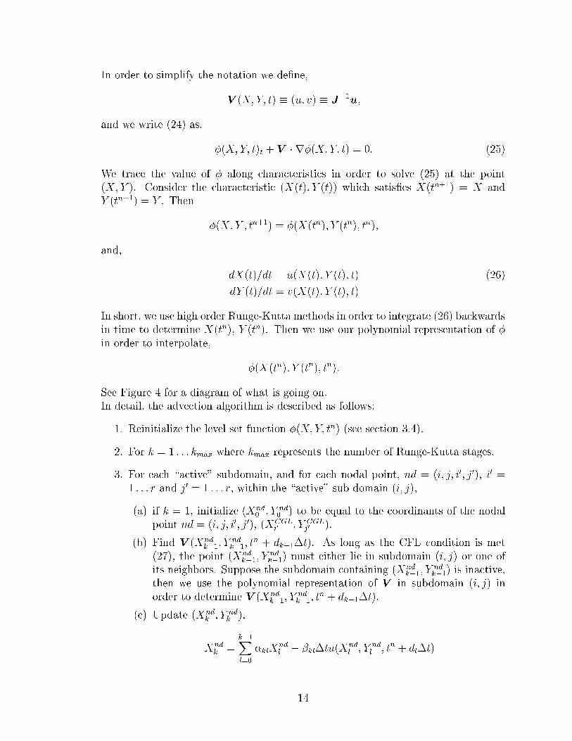
4.3 Normal Adve tionIn table 6 and table 7, we measure the a ura y of our method for normal adve tionof a ir le and normal adve tion of a square where we have s(�) = 1 (2). In Figure8, we display the results for outward normal adve tion of an initial square shape.The physi al domain has dimensions of 100x100. The ir le or square is initially entered at (50; 55). The ir le has a radius of 15 and the square has side of 30 units.5 Con lusionsA dis ontinuous spe tral element method for the level set equation is presented andvalidated. EÆ ien y is gained by implementing a \lo al level set" approa h. Expo-nential onvergen e (i.e., error behaves as Car) is demonstrated for both interfa ialadve tion and for the reinitialization step. Both the interfa e lo ation and urvature onverge exponentially with respe t to the order r (See Tables 1, 2, 3, and 5).Although the order of a ura y of our methodology is higher than onventional�nite di�eren e or �nite element approa hes for adve tion of interfa es, e.g. wedemonstrated fourth order a ura y for adve tion of a ir le, our results do not yetmat h those of front-tra king methods[12℄, parti le methods[22, 15, 21℄, or hybridparti le-level set methods[7℄ when there are sharp orners in the zero level set. Cur-rently, we are in the pro ess of applying this methodology to tra k singular interfa es(sho ks/ onta t dis ontinuities) in gas dynami s. In this framework, where we haveto ouple our adve tion algorithm to the physi s, it is important to have robust repre-sentations of interfa e quantities (e.g. normal and urvature) and it is also importantto be able to robustly extend quantities (e.g. velo ity) a ross interfa es.Sin e our approa h for reinitialization expli itly gives us the losest point on theinterfa e, and also sin e we have lo al polynomial representation of all our variables,we an eÆ iently and robustly derive \spe trally a urate" extension velo ities whi his not possible with urrently available parti le/front-tra king approa hes. Also, ourreinitialization approa h yields spe trally a urate interfa e normal and urvature.

17

Referen es[1℄ D. Adalsteinsson and J.A. Sethian. A level set approa h to a uni�ed modelfor et hing, deposition, and lithography, iii: Re-deposition and re-emission. J.Comput. Phys., 138:193{227, 1997.[2℄ T. Barth. Numeri al methods for gasdynami systems on unstru tured meshes.In Rohde Kroner, Ohlberger, editor, Le ture Notes in omputational s ien e andengineering, pages 195{284. Springer-Verlag, 1998.[3℄ K. Bla k. A onservative spe tral element method for the approximation of ompressible uid ow. Kybernetika, 35(1):133{146, 1999.[4℄ C. Canuto, M.Y. Hussaini, A. Quarteroni, and T.A. Zang. Spe tral methods in uid dynami s. Springer-Verlag, 1988.[5℄ D. Chopp. Some improvements of the fast mar hing method. SIAM J. S i.Comput., 23(1):230{244, 2001.[6℄ B. Co kburn and C.-W. Shu. Tvb runge-kutta lo al proje tion dis ontinuousgalerkin �nite element method for onservation laws ii: general framework. Math-emati s of Computation, 52(186):411{435, 1989.[7℄ D. Enright, R. Fedkiw, R. Ferziger, and I. Mit hell. A hybrid parti le level setmethod for improved interfa e apturing. J. Comp. Phys., 2002. (submitted).[8℄ R. Fedkiw, T. Aslam, and S. Xu. The ghost uid method for de agration anddetonation dis ontinuities. J. Comput. Phys., 154:393{427, 1999.[9℄ J. Helmsen, E.G. Pu kett, P. Colella, and M. Dorr. Two new methods for simu-lating photolithography development in 3d. In Pro eedings of SPIE Opti al/LaserMi rolithography IX, volume 2726, 1996.[10℄ C. Hu and C.-W. Shu. A dis ontinuous galerkin �nite element method forhamilton-ja obi equations. SIAM J. S i. Comput., 21(2):666{690, 1999.[11℄ F. Hu, M.Y. Hussaini, and P. Rasetarinera. An analysis of the dis ontinuousgalerkin method for wave propagation problems. J. Comput. Phys., 151:921{946, 1999.[12℄ D. Juri and G. Tryggvason. Computations of boiling ows. Te hni al ReportLA-UR-97-1145, Los Alamos National Laboratory, 1997.[13℄ D. Kopriva and J. Kolias. A onservative staggered-grid hebyshev multidomainmethod for ompressible ows. J. Comp. Phys., 125:244{261, 1996.[14℄ D. Kopriva, S. Woodru�, and M.Y. Hussaini. Computation of ele tromagnet s attering with a non- onforming dis ontinuous spe tral element method. Intl.Journal for numeri al methods in engineering, 53:105{122, 2002.18

[15℄ Douglas B. Kothe and William J. Rider. A omparison of interfa e tra kingmethods. (manus ript available via anonymous ftp from ), O tober 21 1994.[16℄ R.B. Milne. An adaptive level set method. LBNL te hni al report LBNL-39216,U. C. Berkeley Department of Mathemati s, 1995. PhD thesis.[17℄ S. Osher and J. A. Sethian. Fronts propagating with urvature-dependent speed:Algorithms based on hamilton-ja obi formulations. J. Comput. Phys., 79(1):12{49, 1988.[18℄ P. Rasetarinera and M.Y. Hussaini. An eÆ ient impli it dis ontinuous spe tralgalerkin method. J. Comp. Phys., 172:1{21, 2001.[19℄ P. Rasetarinera, D. Kopriva, and M.Y. Hussaini. Dis ontinuous spe tral elementsolution of a ousti radiation from thin airfoils. AIAA Journal, 39(11):2070{2075, 2001.[20℄ S. Rebay. EÆ ient unstru tured mesh generation by means of delaunay triangu-lation and bowyer-watson algorithm. J. Comput. Phys., 106:125{138, 1993.[21℄ William J. Rider and Douglas B. Kothe. Stret hing and tearing interfa e tra kingmethods. AIAA paper 95-1717, 1995.[22℄ W.J. Rider and D.B. Kothe. Re onstru ting volume tra king. J. Comput. Phys.,141:112{152, 1998.[23℄ J.A. Sethian. A mar hing level set method for monotoni ally advan ing fronts.In Pro . Nat. A ad. S i., volume 93, 1996.[24℄ C.W. Shu and S. Osher. EÆ ient implementation of essentially non-os illatorysho k apturing s hemes, ii. J. Comput. Phys., 83:32{78, 1989.[25℄ V. Smiljanovski, V. Moser, and R. Klein. A apturing-tra king hybrid s hemefor de agration dis ontinuities. Journal of Combustion Theory and Modeling,2(1):183{215, 1997.[26℄ D. Stanes u, M.Y. Hussaini, and F. Farassat. Air raft engine noise s attering-a dis ontinuous spe tral element approa h. In Pro eedings of AIAA, numberAIAA-2002-0800, Reno, NV, 2002.[27℄ N. Sukumar, D. Chopp, and B. Moran. Extended �nite element method andfast mar hing method for three-dimensional fatigue ra k propagation. J. of theMe hani s of Physi s and Solids, 2000. submitted.[28℄ M. Sussman and E.G. Pu kett. A oupled level set and volume of uid methodfor omputing 3d and axisymmetri in ompressible two-phase ows. J. Comp.Phys., 162:301{337, 2000.[29℄ M. Sussman, P. Smereka, and S.J. Osher. A level set approa h for omputingsolutions to in ompressible two-phase ow. J. Comput. Phys., 114:146{159, 1994.19

[30℄ M.A. Taylor, B.A. Wingate, and R.E. Vin ent. An algorithm for omputingfekete points in the triangle. SIAM J. Numer. Anal., 38(5):1707{1720, 2000.[31℄ S. T. Zalesak. Fully multidimensional ux- orre ted transport algorithms for uids. J. Comput. Phys., 31:335{362, 1979.

20

Table 1: Error after reinitialization of ir le.subdomains r EL1 order EL1 order25x25 3 3.5E-5 1.1E-450x50 3 2.6E-6 3.8 7.1E-6 4.0100x100 3 1.4E-7 4.2 8.5E-7 3.125x25 4 1.7E-6 7.9E-650x50 4 4.7E-8 5.2 2.3E-7 5.1100x100 4 1.6E-9 4.9 7.1E-9 5.025x25 5 8.9E-8 4.5E-750x50 5 1.2E-9 6.2 6.4E-9 6.1100x100 5 1.8E-11 6.1 9.1E-11 6.1

21

Table 2: Error in urvature after reinitialization of ir le.subdomains r ECL1 order ECL1 order25x25 3 7.6E-3 2.4E-250x50 3 1.9E-3 2.0 5.6E-3 2.1100x100 3 4.7E-4 2.0 1.3E-3 2.125x25 4 6.4E-4 3.4E-350x50 4 8.3E-5 2.9 4.0E-4 3.1100x100 4 9.8E-6 3.1 5.0E-5 3.025x25 5 4.8E-5 2.7E-450x50 5 3.0E-6 4.0 1.6E-5 4.1100x100 5 1.9E-7 4.0 8.6E-7 4.2

22

Table 3: Error for one full rotation of a ir le.subdomains r EL1 order EL1 order25x25 2 7.9E-2 2.4E-150x50 2 1.6E-2 2.3 4.3E-2 2.5100x100 2 4.0E-3 2.0 9.0E-3 2.325x25 3 2.0E-3 5.2E-350x50 3 2.8E-4 2.8 6.7E-4 3.0100x100 3 3.4E-5 3.0 7.8E-5 3.125x25 4 6.4E-5 1.9E-450x50 4 3.0E-6 4.4 1.0E-5 4.2100x100 4 1.7E-7 4.1 5.1E-7 4.3

23

Table 4: Error for one full rotation of not hed disk (Zalesak's problem).subdomains CFL r EL1 order EL1 order100x100 1/2 3 2.3E-2 N/A 1.1 N/A200x200 1/2 3 9.3E-3 1.3 0.59 0.9200x200 4/5 3 7.3E-3 0.54

24

Table 5: Error in urvature for one full rotation of a ir le.subdomains r ECL1 order ECL1 order25x25 2 9.3E-2 4.2E-150x50 2 4.2E-2 1.1 1.9E-1 1.1100x100 2 2.4E-2 0.8 8.9E-2 1.125x25 3 1.1E-2 5.1E-250x50 3 2.3E-3 2.3 1.1E-2 2.2100x100 3 5.6E-4 2.0 3.2E-3 1.825x25 4 9.9E-4 5.5E-350x50 4 1.2E-4 3.0 8.5E-4 2.7100x100 4 1.2E-5 3.3 1.0E-4 3.1

25

Table 6: Error at t = 15 for normal adve tion of a ir le.subdomains r EL1 order EL1 order25x25 3 1.2E-4 4.4E-450x50 3 1.2E-5 3.3 3.9E-5 3.5

26

Table 7: Error at t = 15 for normal adve tion of a square.subdomains r EL1 order EL1 order25x25 3 2.6E-1 1.450x50 3 6.3E-2 2.0 1.5E-1 3.2100x100 3 3.8E-2 0.7 1.3E-1 0.2200x200 3 1.8E-2 1.1 6.7E-2 1.0

27

List of Figures1 Interpolatory points for the Ja obian matrix orrespond to the \Leg-endre Gauss" points; r = 3. . . . . . . . . . . . . . . . . . . . . . . . 292 Positioning of the interpolatory points for the level set fun tion andfor the adve tive velo ity �eld when r = 3. The interpolatory pointsin this diagram orrespond to the \Chebyshev Gauss-Lobatto" pointswhi h overlap at subdomain boundaries. . . . . . . . . . . . . . . . . 303 Figure depi ting a sample sten il for reating the height fun tion. . . 314 Figure depi ting ba kwards tra ing of hara teristi s. . . . . . . . . 325 Dis ontinuous Galerkin solution to Zalesak's problem after one fullrevolution of not hed disk. CFL=1/2. Grid resolution is 100x100. . . 336 Dis ontinuous Galerkin solution to Zalesak's problem after one fullrevolution of not hed disk. CFL=1/2. Grid resolution is 200x200. . . 347 Dis ontinuous Galerkin solution to Zalesak's problem after one fullrevolution of not hed disk. CFL=4/5. Grid resolution is 200x200. . . 358 Dis ontinuous Galerkin solution to outward normal adve tion of asquare. Grid resolution is 50x50, r = 3. . . . . . . . . . . . . . . . . 36

28

f ff f ff f fff f fff ff fff ff f ff f fff ff f ff f fff ff f ff f fff ff f ff f fff f fff ff ff f f fff ff fff ff f ff f ff Figure 1:

29

h h h hhhhh hh hhh hhh h h h hhhhhhhhh hhh

hhhhhhh hhhhhhhh h

hhhhh hhhhh hhhhhh hhhhhhhhh hhhh h hhhh

hhhh h hhhhhhhhhhhhhhhhFigure 2:

30

Element (i,j)

LS>0 above y=h(x)

LS<0 below y=h(x)

(r+1,jlo(r+1))(2,jcrit(2))

(i,j), i’=3, j’=2

node (i’,j’) of element

(1,jlo(1))

Figure 3:

31

inactive

inactive inactive

y=h(x)

direction of flow

direction of flow

element (i,j)

characteristic traces backfrom (i-1,j-2,3,3) intothe inactive subdomain (i,j-2)

Characteristic traces backfrom (i,j-1,3,2) into subdomain(i+1,j-1)Figure 4:

32

t=628 100x100 Figure 5:33

t=628 200x200 Figure 6:34

t=628 200x200 Figure 7:35

t=15.0 50x50 Figure 8:36