Embed Size (px)
Citation preview


DISCLAIMER
United States Government. Neither the United States Government nor any agencythereof, nor Battelle Memorial Institute, nor any of their employees, makesanywarranty, express or implied, or assumes any legal liability or responsibilityfor the accuracy, completeness, or usefulness of any information, apparatus,product, or process disclosed, or represents that its use would not infringeprivately owned rights. Reference herein to any specific commercial product,process, or service by trade name, trademark, manufacturer, or otherwise doesnot necessarily constitute or imply its endorsement, recommendation, or favoringby the United States Government or any agency thereof, or Battelle MemorialInstitute. The views and opinions of authors expressed herein do not necessarilystate or reflect those of the United States Government or any agency thereof.
PACIFIC NORTHWEST NATIONAL LABORATORYoperated byBATTELLE
for theUNITED STATES DEPARTMENT OF ENERGY
under Contract DE-AC06-76RLO1830
Printed in the United States of America
Available to DOE and DOE contractors from theOffice of Scientific and Technical Information,
P.O. Box 62, Oak Ridge, TN 37831-0062;ph: (865) 576-8401fax: (865) 576-5728
email: [email protected]
Available to the public from the National Technical Information Service,U.S. Department of Commerce, 5285 Port Royal Rd., Springfield, VA 22161
ph: (800) 553-6847fax: (703) 605-6900
email: [email protected] ordering: http://www.ntis.gov/ordering.htm
This document was printed on recycled paper.(8/00)

PNNL-14779
Six-Degree-of-Freedom Sensor Fish Design:Governing Equations and Motion Modeling
Z. DengM. C. RichmondC. S. SimmonsT. J. Carlson
July 2004
Prepared for the U.S. Department of Energyunder Contract DE-AC06-76RL01830
Pacific Northwest National LaboratoryRichland, Washington 99352

Executive Summary
The Sensor Fish device is being used at Northwest hydropowerprojects to better understandthe conditions fish experience during passage through hydroturbines and other dam bypass alter-natives. Since its initial development in 1997, the Sensor Fish has undergone numerous designchanges to improve its function and extend the range of its use. The most recent Sensor Fish de-sign, the three degree of freedom (3DOF) device, has been used successfully to characterize theenvironment fish experience when passing through turbines,in spill, or in engineered fish bypassfacilities at dams.
Pacific Northwest National Laboratory (PNNL) is in the process of redesigning the current3DOF Sensor Fish device package to improve its field performance. Rate gyros will be added tothe new six degree of freedom (6DOF) device so that it will be possible to observe the six linearand angular accelerations of the Sensor Fish as it passes thedam. Before the 6DOF Sensor Fishdevice can be developed and deployed, governing equations of motion must be developed in orderto understand the design implications of instrument selection and placement within the body of thedevice.
In this report, we describe a fairly general formulation forthe coordinate systems, equations ofmotion, force and moment relationships necessary to simulate the the 6DOF movement of an un-derwater body. Some simplifications are made by consideringthe Sensor Fish device to be a rigid,axisymmetric body. The equations of motion are written in the body-fixed frame of reference.Transformations between the body-fixed and inertial reference frames are performed using a for-mulation based on quaternions. Force and moment relationships specific to the Sensor Fish bodyare currently not available. However, examples of the trajectory simulations using the 6DOF equa-tions are presented using existing low and high-Reynolds number force and moment correlations.Animation files for the test cases are provided in an attachedCD.
The next phase of the work will focus on the refinement and application of the 6DOF simulatordeveloped in this project. Experimental and computationalstudies are planned to develop a set offorce and moment relationships that are specific to the Sensor Fish body over the range of Reyn-olds numbers that it experiences. Lab testing of prototype 6DOF Sensor Fish will also allow forrefinement of the trajectory simulations through comparison with observations in test flumes. The6DOF simulator will also be an essential component in tools to analyze field data measured usingthe next generation Sensor Fish. The 6DOF simulator will be embedded in a moving-machinerycomputational fluid dynamics (CFD) model for hydroturbines to numerically simulate the 6DOFSensor Fish.
iii

Acknowledgments
The authors are grateful for the contributions and input of many people on this project. JohnSerkowski and Bill Perkins provided technical help preparing the manuscript. Georganne O’Connorand Jennifer Zohn were the technical editors for this document. Dennis Dauble’s involvement andoversight was also greatly appreciated. Finally, we would like to thank the U.S. Department ofEnergy’s Wind and Hydropower Program for funding this study.
v

Contents
Executive Summary. . . . . . . . . . . . . . . . . . . . . . . . . . . . . . . . . . . . . iii
Acknowledgments. . . . . . . . . . . . . . . . . . . . . . . . . . . . . . . . . . . . . . v
1.0 Introduction. . . . . . . . . . . . . . . . . . . . . . . . . . . . . . . . . . . . . . . 1
2.0 Governing Equations of Rigid Body Motion. . . . . . . . . . . . . . . . . . . . . . 3
2.1 Coordinate Systems and Transformations . . . . . . . . . . . . . .. . . . . . . . 3
2.2 Rigid-Body Dynamics . . . . . . . . . . . . . . . . . . . . . . . . . . . . . . . .6
3.0 Forces and Coefficients Evaluation. . . . . . . . . . . . . . . . . . . . . . . . . . . 11
3.1 Flow Field . . . . . . . . . . . . . . . . . . . . . . . . . . . . . . . . . . . . . . .11
3.2 Hydrostatics . . . . . . . . . . . . . . . . . . . . . . . . . . . . . . . . . . . .. . 13
3.3 Added Mass . . . . . . . . . . . . . . . . . . . . . . . . . . . . . . . . . . . . . .14
3.4 Drag Forces and Moments . . . . . . . . . . . . . . . . . . . . . . . . . . . .. . 17
3.4.1 Axial Drag Coefficients . . . . . . . . . . . . . . . . . . . . . . . . . . .17
3.4.2 Cross-Flow Drag Coefficients . . . . . . . . . . . . . . . . . . . . . . .. 18
3.4.3 Total Drag Forces and Moments . . . . . . . . . . . . . . . . . . . . .. . 19
3.5 Lift Forces and Moments . . . . . . . . . . . . . . . . . . . . . . . . . . . .. . . 20
3.6 Resultant Forces and Moments . . . . . . . . . . . . . . . . . . . . . . . .. . . . 21
4.0 Simulation . . . . . . . . . . . . . . . . . . . . . . . . . . . . . . . . . . . . . . . 23
4.1 Complete Equations of 6DOF Motion . . . . . . . . . . . . . . . . . . . .. . . . 23
4.2 Numerical Simulation . . . . . . . . . . . . . . . . . . . . . . . . . . . . .. . . . 24
4.3 Test Examples . . . . . . . . . . . . . . . . . . . . . . . . . . . . . . . . . . . .. 25
vii

4.3.1 Terminal Settling Velocity of a Falling Sphere in a Viscous Fluid . . . . . . 25
4.3.2 Motion of an Ellipsoid at Low Reynolds Numbers . . . . . . . .. . . . . 25
4.3.3 Six Degree of Freedom Motion of Sensor Fish . . . . . . . . . .. . . . . 29
5.0 Summary. . . . . . . . . . . . . . . . . . . . . . . . . . . . . . . . . . . . . . . . 37
6.0 References. . . . . . . . . . . . . . . . . . . . . . . . . . . . . . . . . . . . . . . 39
Appendix A: Ellipsoid Motion Equations for Low Reynolds Numbers . . . . . . . . . . . A.1
Appendix B: Nomenclature. . . . . . . . . . . . . . . . . . . . . . . . . . . . . . . . B.1
viii

Figures
2.1 Sensor Fish body-fixed and inertial coordinate systems .. . . . . . . . . . . . . . 4
3.1 Drag coefficients as a function of Reynolds number for a smooth cylinder andsphere: (a) plotted in log scale; (b) plotted in linear scale. . . . . . . . . . . . . . 19
4.1 Terminal velocity of a sphere at Re<< 1 . . . . . . . . . . . . . . . . . . . . . . 26
4.2 Trajectory of an ellipsoid in a 1-m-wide parabolic velocity field . . . . . . . . . . . 27
4.3 Ellipsoid Trajectory Components in 1-m-wide parabolic shear flow. Ellipsoid isinitially turned 45 degrees to the flow direction, toward theflow center. Rotationis about the inertial Z-axis. . . . . . . . . . . . . . . . . . . . . . . . . . .. . . . 28
4.4 Ellipsoid Trajectory Components in 10-m-wide parabolicshear flow. Ellipsoid isinitially turned 45 degrees into flow direction, toward the flow center. Rotation isabout the inertial Z-axis. . . . . . . . . . . . . . . . . . . . . . . . . . . . .. . . 28
4.5 Ellipsoid Trajectory Components in 10-m-wide parabolicshear flow. Ellipsoid isinitially turned 45 degrees into flow direction, toward the flow center. Rotation isabout the inertial Z-axis. With the direction of gravity points in the same directionof flow. . . . . . . . . . . . . . . . . . . . . . . . . . . . . . . . . . . . . . . . .29
4.6 Trajectory of Sensor Fish for case 1, (a) x(t), y(t), and z(t); (b) θ(t) . . . . . . . . . 31
4.7 A snapshot of 6DOF motion of Sensor Fish . . . . . . . . . . . . . . .. . . . . . 31
4.8 Trajectory of Sensor Fish for case 2 in one-dimensional uniform flow with an offsetbetween mass center and geometric center of Sensor Fish, (a)x(t), y(t), and z(t);(b) θ(t) . . . . . . . . . . . . . . . . . . . . . . . . . . . . . . . . . . . . . . . .32
4.9 Trajectory of Sensor Fish for case 3 in one-dimensional uniform flow with masscenter and geometric center of Sensor Fish overlapped, (a) x(t), y(t), and z(t); (b)θ(t) . . . . . . . . . . . . . . . . . . . . . . . . . . . . . . . . . . . . . . . . . .32
4.10 Trajectory of Sensor Fish for case 4 in two-dimensionaluniform flow with an offsetbetween mass center and geometric center of Sensor Fish, (a)x(t), y(t), and z(t);(b) θ(t) . . . . . . . . . . . . . . . . . . . . . . . . . . . . . . . . . . . . . . . .33
ix

4.11 Trajectory of Sensor Fish for case 5 in two-dimensionaluniform flow with masscenter and geometric center of Sensor Fish overlapped, (a) x(t), y(t), and z(t); (b)θ(t) . . . . . . . . . . . . . . . . . . . . . . . . . . . . . . . . . . . . . . . . . .33
4.12 Trajectory and angular velocity of Sensor Fish for case6 in parabolic flow fieldwith an offset between mass center and geometric center of Sensor Fish, (a) x(t),y(t), and z(t); (b) y(t); (c)θ(t); (d) p(t), q(t), r(t) . . . . . . . . . . . . . . . . . . . 34
4.13 Trajectory and angular velocity of Sensor Fish for case7 in parabolic flow fieldwith mass center and geometric center of Sensor Fish overlapped, (a) x(t), y(t),and z(t); (b) y(t); (c)θ(t); (d) p(t), q(t), r(t) . . . . . . . . . . . . . . . . . . . . . .35
x

1.0 Introduction
Hydropower is a major producer of renewable, non-carbon based, “green” electrical power.However, hydropower production impacts fish that live in or migrate through impounded riversystems. In the Pacific Northwest and elsewhere, improvement in the survival and reduction inthe injury rate for fish passing through turbines is being sought through changes in hydroturbinedesign and in hydroturbine operation. An additional goal isproduction of more electrical power athigher efficiency. Evidence to date indicates these goals are complementary.
The Sensor Fish device (Sensor Fish) is an autonomous devicebeing used to better understandthe physical conditions fish experience during passage through hydroturbines and other dam bypassalternatives. Sensor Fish development was initiated at Pacific Northwest National Laboratory in1997 as an internal development initiative. The product of the initiative was a functional prototypethat was field tested in spring 1999 and extensively used during winter 1999-2000 as part of anevaluation of the first minimum gap runner installed at Bonneville Dam’s first powerhouse on theColumbia River. The purpose of these field tests was to assess physical damage caused by turbinepassage and develop retrieval methods for the Sensor Fish from the tailrace. Since this initial use,the Sensor Fish has undergone numerous design changes to improve its function and extend therange of its use (Carlson et al. 2003; Carlson and Duncan 2003).
The most recent and ambitious extension of function of the Sensor Fish is the current projectto add rate gyros to the linear accelerometers which always have been an element of the SensorFish package. Adding the rate gyros will permit all six possible motions of the Sensor Fish (threecomponents of linear acceleration plus pitch, roll, and yawangles) to be observed.
In actual use, the Sensor Fish is only one part of a “system” necessary to acquire data onhydraulic forces. There are other requirements related to deploying and retrieving the Sensor Fish,downloading acquired data, and analyzing and interpretingdata. The new Sensor Fish will greatlyextend the capabilities of this “system” in many ways. The new sensor package will make itpossible for all six degrees of freedom (6DOF) required to describe the motion of a rigid body tobe obtained for the Sensor Fish during transit through a hydroturbine or other dam passage route.
The goals of the 6DOF Sensor Fish system project are to:
1. Redesign the 3DOF Sensor Fish to incrementally improve overall Sensor Fish field per-formance and add rate gyros to provide full 6DOF measurementcapability. Some moreimportant design changes include the following:
• increased analog to digital sampling frequency
• more non-volatile internal memory for data storage
• linear accelerometers with increased dynamic range
• software access to turn the battery on and off and to initiatea charging cycle
1

• rigid mounting of sensor packages on printed circuit cards
• pressure sensor with smaller external opening and greater sensitivity.
2. Implement a numerical model of the 6DOF Sensor Fish withina particle-tracking modulefor use with Computational Fluid Dynamics (CFD), moving machinery simulation of hydro-turbines.
3. Analyze Sensor Fish data sets and movement simulation software.
In order to achieve these goals, it is first necessary to develop governing equations for the6DOF motion for a rigid body. The 6DOF equations of motion (6DOF-EOM) described in thisreport will be used to achieve several critical steps in the design and implementation of the 6DOFSensor Fish. First, the 6DOF-EOM will be used to evaluate elements of the 6DOF Sensor Fishdesign. It is essential that the impact on the device motion caused by basic mechanical featuresof the 6DOF Sensor Fish, particularly the sensor’s mass distribution and buoyancy characteristics,are taken into account in the design process.
Second, the 6DOF-EOM will be incorporated into particle-tracking software to numericallysimulate the 6DOF Sensor Fish. This approach already has been used. The current 3DOF particle-tracking capability has been used byRichmond et al.(2004) to help analyze and understand 3DOFSensor Fish data sets and extend analysis of live fish data acquired to assess the biological perfor-mance of spill for fish passage at The Dalles Dam.
Third, the 6DOF-EOM will serve as the base of software developed to analyze 6DOF Sen-sor Fish data sets. Using the 6DOF-EOM in this way will optimize extraction of information forcharacterizing fish passage conditions from Sensor Fish data sets. In particular, improved data-analysis methods are needed to detect and describe Sensor Fish response to exposure conditions,such as strike, scraping, and shear, events which are the primary injury mechanisms for fish passingthrough turbines. These developments will permit better use of Sensor Fish data sets and provideimproved understanding of the location and dynamics of conditions deleterious to fish during tur-bine, spill, and bypass passage.
In Section 2 of this report, the equations of motion for an underwater body are written inthe body-fixed frame of reference. Section 3 presents force and moment relationships that, whilenot specifc to the Sensor Fish body, are useful approximations that are used in Section 4 to showexamples of the trajectory simulations using the 6DOF equations. Animation files for the test casesare provided in an attached CD.
2

2.0 Governing Equations of Rigid Body Motion
This chapter defines the coordinate systems and governing equations related to the motion ofSensor Fish. To simplify the derivation of the equations, itis assumed that Sensor Fish are rigid andcylindrical. Therefore, the terms “Sensor Fish” and “rigidbody” are interchangeable throughoutthe report, even though the formulation is general and can beapplied to other body shapes such assphere and ellipsoids.
2.1 Coordinate Systems and Transformations
“Body-fixed coordinate system (frame)” and “inertial coordinate system (frame)” are termsused in this report. The origin of the body-fixed coordinate system is located at the center ofbuoyancy (center of geometry). Figure2.1 illustrates the definition of the two systems. There arevarious ways to describe the general motion of a rigid body in6DOF. Conventional aerodynamicsdefinitions are used in the current investigation.
Suppose(x, y, z) and(φ, θ, ψ) are the position and orientation of Sensor Fish with respectto theinertial coordinate system. In aerodynamics, the Euler anglesφ, θ andψ are usually labeled as yaw,pitch, and roll angles, respectively, which can be determined by the following steps: (1) roll angleψ is obtained by rotating inertial system about its z-axis until its y-axis becomes perpendicular tothe plane of the inertial z-axis and the body-fixed x-axis; (2) pitch angleθ is obtained by rotatingthe new inertial system (created by step 1) about its new y-axis until its x-axis overlaps with thebody-fixed x-axis; (3) yaw angleφ is finally obtained by continuing to rotate the new inertial system(now created by step
2) about its new x-axis until its y-axis lines up with the body-fixed y-axis. The correspondinghomogeneous transformationA is defined as
A = R(z,ψ)R(y,θ)R(x,φ)
=
cosθcosψ sinψcosθ −sinθcosψsinθsinφ−sinψcosφ sinψsinθsinφ+cosψcosφ cosθsinφcosψsinθcosφ+sinψsinφ sinψsinθcosφ−cosψsinφ cosθcosφ
, (2.1)
which is orthogonal and transforms translational velocities between the inertial and body-fixedcoordinate systems by
xyz
= A−1
uvw
= AT
uvw
, (2.2)
where(u, v, w)T and(x, y, z)T are the translational velocity of Sensor Fish with respect to thebody-fixed coordinate system and the inertial system, respectively.
3

Figure 2.1. Sensor Fish body-fixed and inertial coordinate systems
Components of the angular velocity in the body-fixed system can be expressed in terms of theorientation angles and their derivatives
pqr
=
φ− ψsinθθcosφ+ ψsinφcosθψcosφcosθ− θsinφ
=
1 0 −sinθ0 cosφ sinφcosθ0 −sinφ cosφcosθ
φθψ
, (2.3)
where(p, q, r)T and(φ, θ, ψ)T are the rotational velocities of Sensor Fish with respect tothebody-fixed coordinate system and the inertial system, respectively. Therefore, by computing theinverse of the transformation matrix in Equation (2.3), we can define the transformation matrix ofangular velocity,J,
φθψ
= J
pqr
, (2.4)
4
where
J =
1 sinφ tanθ cosφ tanθ0 cosφ −sinφ0 sinφ/cosθ cosφ/cosθ
. (2.5)
For the second transformation matrixJ, there are singularities at cosθ = 0, that is, when theSensor Fish has a pitch angleθ = ±90, the coordinate transform based on roll, pitch, and yawangles doesn’t work anymore. This singlarity associated with the use of Euler angles is sometimesreferred to as “gimbal-lock”. To overcome this deficiency, the quaternion representation for rigidbody rotation is introduced.
Let four parametersε1, ε2, ε3, andε4 form the components of the quaternionε, as follows:
ε =
ε1ε2ε3ε4
. (2.6)
The general rotation of a rigid body has only three degrees offreedom, so the four componentsare not independent and satisfy the constraint equation
ε21 + ε2
2 + ε23 + ε2
4 = 1. (2.7)
The related transformation matrixQ in terms of quaternion components is given by
Q(ε) =
ε21− ε2
2− ε23 + ε2
4 2(ε1ε2 + ε3ε4) 2(ε1ε3− ε2ε4)2(ε1ε2− ε3ε4) −ε2
1 + ε22− ε2
3 + ε24 2(ε2ε3 + ε1ε4)
2(ε1ε3 + ε2ε4) 2(ε2ε3− ε1ε4) −ε21− ε2
2 + ε23 + ε2
4
=
1−2(ε22 + ε2
3) 2(ε1ε2 + ε3ε4) 2(ε1ε3− ε2ε4)2(ε1ε2− ε3ε4) 1−2(ε2
1 + ε23) 2(ε2ε3 + ε1ε4)
2(ε1ε3 + ε2ε4) 2(ε2ε3− ε1ε4) 1−2(ε21 + ε2
2)
. (2.8)
For a given homogeneous transformation matrixA as defined in Equation (2.1), quaternionεcan be computed from
A = Q(ε1, ε2, ε3, ε4) (2.9)
ε4 = ±12
√
1+A1,1 +A2,2 +A3,3, (2.10)
if ε4 6= 0, then
ε1 =1
4ε4(A2,3−A3,2)
ε2 =1
4ε4(A3,1−A1,3) (2.11)
ε3 =1
4ε4(A1,2−A2,1);
5

if ε4 = 0, then
ε1 =12
√
1+A1,1−A2,2−A3,3
ε2 =12
√
1−A3,3−2ε21 (2.12)
ε3 =12
√
1−A2,2−2ε21.
Note there is a sign ambiguity in the calculation of these components. As a result, there are atleast two sets of quaternion parameters. However, the equivalent transformation matrixQ(ε) is thesame becauseQ(ε) (see Equation [2.8]) is not affected by the simultaneous change of signs of thefour components.
The time derivative of the quaternion is related to the rotational velocities in the body-fixedframe,
ε1ε2ε3ε4
=
dε1/dtdε2/dtdε3/dtdε4/dt
=12
0 r −q p−r 0 p qq −p 0 r−p −q −r 0
ε1ε2ε3ε4
(2.13)
wheret is the time. Refer toHughes(1986) or Maxey and Riley(1983) for more details of quater-nion representation.
On the other hand, for a given quaternionε, the transformation matrixQ(ε) is computed fromEquation (2.8), and the related orientation angles can be obtained from
θ = arcsin(−Q1,3)
φ = arctanQ2,3
Q3,3(2.14)
ψ = arctanQ1,2
Q1,1
2.2 Rigid-Body Dynamics
Because most of the external forces and moments exerted on theSensor Fish are representedin the body-fixed system, all the governing equations of motion will be written in the body-fixedsystem as well.
Define
v =
uvw
, a =dvdt
=
uvw
, Ω =
pqr
,dΩdt
=
pqr
, (2.15)
rg =
xgygzg
, ∑F =
∑FX
∑FY
∑FZ
, ∑M =
∑MX
∑MY
∑MZ
, (2.16)
6
where(xg,yg,zg) is the center of mass in the body-fixed frame, that is, the offset of the center ofmass with respect to the center of buoyancy because the origin of the body-fixed frame is definedat the center of buoyancy;∑F and∑M are the total force and moment exerted on the body, and allthe components and operations are with respect to the body-fixed frame.
Use vector operation to compute the velocityvg and accelerationag at the center of mass in thebody-fixed frame, and note that the origin of body-fixed frameis defined at the center of buoyancy,
vg =drg
dt= v+Ω× rg, (2.17)
then,
ag =dvg
dt=
ddt
(v+Ω× rg)
=dvdt
+ddt
(Ω× rg)
=dvdt
+dΩdt
× rg +Ω× drg
dt
=dvdt
+dΩdt
× rg +Ω× (v+Ω× rg). (2.18)
Use Newton’s second law to relate the external forces to linear acceleration,
∑F = mag = m
(
dvdt
+dΩdt
× rg +Ω×v+Ω× (Ω× rg)
)
. (2.19)
Similarly, use Euler’s equation to relate the external moments to rotational motion of the rigidbody,
∑M = mrg× (dvdt
+Ω×v)+ I · dΩdt
+Ω× (I ·Ω), (2.20)
wherem is the mass of the rigid body, and
I =
Ixx −Ixy −Ixz−Ixy Iyy −Iyz−Ixz −Iyz Izz
(2.21)
is the inertial tensor, in which(Ixx, Iyy, Izz) are the moments of inertia and the other components areusually referred to as the products of inertia.
Expand Equations (2.19) and (2.20), and obtain the general governing equations of a rigid body
7

in the body-fixed frame with its origin located at the center of buoyancy:
∑FX = m[
u−vr +wq−xg(q2 + r2)+yg(pq− r)+zg(pr + q)
]
∑FY = m[
v−wp+ur−yg(p2 + r2)+zg(qr− p)+xg(pq+ r)]
∑Fz = m[
w−uq+vp−zg(p2 +q2)+xg(pr− q)+yg(qr + p)]
∑MX = Ixxp+(Izz− Iyy)qr− Ixz(r + pq)+ Iyz(r2−q2)+ Ixy(pr− q)
+m[yg(w−uq+vp)−zg(v−wp+ur)] (2.22)
∑MY = Iyyq+(Ixx− Izz)pr− Ixy(p+qr)+ Izx(p2− r2)+ Iyz(pq− r)
+m[zg(u−vr +wq)−xg(w−uq+vp)]
∑MZ = Izzr +(Iyy− Ixx)pq− Iyz(q+ pr)+ Ixy(q2− p2)+ Ixz(rq− p)
+m[xg(v−wp+ur)−yg(u−vr +wq)]
The governing equations can be re-written in a matrix form,
∑FX
∑FY
∑FZ
∑MX
∑MY
∑MZ
=
m 0 0 0 mzg −myg
0 m 0 −mzg 0 mxg
0 0 m myg −mxg 00 −mzg myg Ixx −Ixy −Ixz
mzg 0 −mxg −Ixy Iyy −Iyz
−myg mxg 0 −Ixz −Iyz Izz
·
uvwpqr
+
0 0 0 m(zgr +ygq) m(w−xgq) −m(v+xgr)0 0 0 m(w−ygp) m(zgr −ygq) m(u−ygr)0 0 0 −m(v+xgr) m(ygr −u) −m(xgp+ygq)
−m(ygq+zgr) m(w+ygp) m(zgp−v) 0 Izzr − Iyzq− Ixzp Iyzr + Ixxp− Iyyqm(xgq−w) −m(zgr +xgp) m(zgq+u) Iyzq+ Ixzp+ Izzr 0 Ixxp− Ixzr − Ixyqm(xgr +v) m(ygr −u) −m(xgp+ygq) Iyyq− Ixyp− Iyzr Ixyq+ Ixzr − Ixxp 0
·
uvwpqr
Normalize the equations with the mass of the rigid body, get
∑F ′X
∑F ′Y
∑F ′Z
∑M′X
∑M′Y
∑M′Z
=
1 0 0 0 zg −yg
0 1 0 −zg 0 xg
0 0 1 yg −xg 00 −zg yg I ′xx −I ′xy −I ′xz
zg 0 −xg −I ′xy I ′yy −I ′yz
−yg xg 0 −I ′xz −I ′yz I ′zz
·
uvwpqr
+
0 0 0 (zgr +ygq) (w−xgq) −(v+xgr)0 0 0 (w−ygp) (zgr −ygq) (u−ygr)0 0 0 −(v+xgr) (ygr −u) −(xgp+ygq)
−(ygq+zgr) (w+ygp) (zgp−v) 0 I ′zzr − I ′yzq− I ′xzp I′yzr + I ′xxp− I ′yyq(xgq−w) −(zgr +xgp) (zgq+u) I ′yzq+ I ′xzp+ I ′zzr 0 I ′xxp− I ′xzr − I ′xyq(xgr +v) (ygr −u) −(xgp+ygq) I ′yyq− I ′xyp− I ′yzr I ′xyq+ I ′xzr − I ′xxp 0
·
uvwpqr
8

where
∑F ′X
∑F ′Y
∑F ′Z
∑M′X
∑M′Y
∑M′Z
=
∑FX/m∑FY/m∑FZ/m∑MX/m∑MY/m∑MZ/m
(2.23)
and
I ′ =
I ′xx −I ′xy −I ′xz−I ′xy I ′yy −I ′yz−I ′xz −I ′yz I ′zz
= I/m=
Ixx/m −Ixy/m −Ixz/m−Ixy/m Iyy/m −Iyz/m−Ixz/m −Iyz/m Izz/m
(2.24)
9

3.0 Forces and Coefficients Evaluation
For the equations of a rigid-body motion in a water flow field, the total forces and moments are
∑F = FHS +FL +FD +FA +FP
∑M = MHS +ML +MD +MA +MP (3.1)
whereFHS andMHS are hydrostatic forces and moments,FL andML are body lift forces andmoments,FD and MD are body hydrodynamic drag forces and moments,FA and MA are thecorresponding forces and moments of added mass, andFP and MP are propulsion forces andmoments.
In the current investigation, no propulsion is assumed, i.e., MP = 0, FP = 0, so Equation (3.1)becomes
∑F = FHS +FL +FD +FA
∑M = MHS +ML +MD +MA (3.2)
3.1 Flow Field
Suppose the ambient flow field has velocity (Vx, Vy, Vz) in the inertial frame; then the angularvelocity is defined as
ωx = 12
(
∂Vz∂y − ∂Vy
∂z
)
ωy = 12
(
∂Vx∂z − ∂Vz
∂x
)
(3.3)
ωz = 12
(
∂Vy∂x − ∂Vx
∂y
)
In the body-fixed frame they are transformed to
V1(ε)V2(ε)V3(ε)
= Q(ε) ·
Vx
Vy
Vz
=
VxQ1,1(ε)+VyQ1,2(ε)+VzQ1,3(ε)VxQ2,1(ε)+VyQ2,2(ε)+VzQ2,3(ε)VxQ3,1(ε)+VyQ3,2(ε)+VzQ3,3(ε)
(3.4)
ω1(ε)ω2(ε)ω3(ε)
= Q(ε) ·
ωx
ωy
ωz
=
ωxQ1,1(ε)+ωyQ1,2(ε)+ωzQ1,3(ε)ωxQ2,1(ε)+ωyQ2,2(ε)+ωzQ2,3(ε)ωxQ3,1(ε)+ωyQ3,2(ε)+ωzQ3,3(ε)
(3.5)
11

where
V1(ε)V2(ε)V3(ε)
and
ω1(ε)ω2(ε)ω3(ε)
are the translational velocity and angular velocity of the ambient
flow field in the body-fixed frame.
Define gradient tensor of the ambient velocity in the inertial frame,
∇Ve =
∂Vx∂x
∂Vx∂y
∂Vx∂z
∂Vy∂x
∂Vy∂y
∂Vy∂z
∂Vz∂x
∂Vz∂y
∂Vz∂z
(3.6)
and in the body-fixed frame, it becomes
∇Vb = Q · (∇Ve) ·Q−1 (3.7)
where the subscripts b and e relate to the body-fixed frame andthe earth-fixed (inertial) frame,respectively.
The time derivative of the transformation matrixQ is
Qi, j =∂Qi, j
∂ε1ε1 +
∂Qi, j
∂ε2ε2 +
∂Qi, j
∂ε3ε3 +
∂Qi, j
∂ε4ε4, i, j = 1,2,3 (3.8)
where
ε1
ε2
ε3
ε4
=12
0 r −q p−r 0 p qq −p 0 r−p −q −r 0
ε1
ε2
ε3
ε4
(3.9)
Now evaluate the acceleration of the flow velocity in the body-fixed frame,
V1
V2
V3
= Q ·
Vx
Vy
Vz
+ Q ·
Vx
Vy
Vz
= Q ·
∇Ve ·
xyz
+∂∂t
Vx
Vy
Vz
+ Q ·
Vx
Vy
Vz
= Q · (∇Ve) ·Q−1 ·
uvw
+Q · ∂∂t
Vx
Vy
Vz
+ Q ·
Vx
Vy
Vz
(3.10)
= ∇Vb ·
uvw
+Q · ∂∂t
Vx
Vy
Vz
+ Q ·
Vx
Vy
Vz
(3.11)
Computing the rate of change of the flow angular velocity in thebody-fixed frame requiresdifferentiating∇Vb with respect to time. This will also require introducing second order spatial
12

partial derivatives of the flow velocity in the inertial frame. The time derivative is
d∇Vb
dt= Q ·∇Ve ·Q−1 +Q · d∇Ve
dt·Q−1 +Q ·∇Ve · (Q)−1 (3.12)
where
d∇Ve
dt=
(
∂∇Ve
∂x,∂∇Ve
∂y,∂∇Ve
∂z
)
·
xyz
+∂∇Ve
∂t(3.13)
Finally, the rate of change of the ambient angular velocity in the body-fixed frame is obtainedas follows:
ω1 =12
(
d(∇Vb)r,q
dt− d(∇Vb)q,r
dt
)
ω2 =12
(
d(∇Vb)p,r
dt− d(∇Vb)r,p
dt
)
(3.14)
ω3 =12
(
d(∇Vb)q,p
dt− d(∇Vb)p,q
dt
)
3.2 Hydrostatics
Hydrostatic forces include body weight(W) and buoyancy(B). In the inertial frame,
W =
00W
, B =
00B
(3.15)
Note the governing equations are with respect to body-fixed coordinate system and by applyingthe quaternion transformation matrix defined in Equation (2.8), express the hydrostatic forces andmoments in the body-fixed frame as
W(ε) = Q(ε) ·
00W
, B(ε) = Q(ε) ·
00B
(3.16)
FHS(ε) =
XHS(ε)YHS(ε)ZHS(ε)
= W(ε)−B(ε) =
(W−B)Q1,3(ε)(W−B)Q2,3(ε)(W−B)Q3,3(ε)
(3.17)
MHS(ε) =
KHS(ε)MHS(ε)NHS(ε)
=
xg
yg
zg
× W(ε)−
xb
yb
zb
× B(ε)
=
(ygW−ybB)Q3,3(ε)− (zgW−zbB)Q2,3(ε)(zgW−zbB)Q1,3(ε)− (xgW−xbB)Q3,3(ε)(xgW−xbB)Q2,3(ε)− (ygW−ybB)Q1,3(ε)
(3.18)
13

where(xb,yb,zb) is the center of buoyancy in the body-fixed frame.
As defined earlier, the origin of body-fixed coordinate system is at the center of buoyancy, thatis, xb = yb = zb = 0, so the final expressions for hydrostatic forces and moments are
(
FHS(ε)MHS(ε)
)
=
XHS(ε)YHS(ε)ZHS(ε)KHS(ε)MHS(ε)NHS(ε)
=
(W−B)Q1,3(ε)(W−B)Q2,3(ε)(W−B)Q3,3(ε)
ygWQ3,3(ε)−zgWQ2,3(ε)zgWQ1,3(ε)−xgWQ3,3(ε)xgWQ2,3(ε)−ygWQ1,3(ε)
(3.19)
3.3 Added Mass
When a rigid body accelerates within a fluid field, some amount of surrounding fluid moveswith the body. Added mass is a measure of this moving fluid and relates the linear and angularacceleration to the hydrodynamics forces exerted by the moving fluid. As noted byMougin andMagnaudet(2002) added-mass effects are independent of Reynolds number and whether the flowis steady or unsteady.Newman(1977) derived the forces and moments for ideal fluid due to theadded mass in a stationary flow field,
(FA) j = − ˙vimji − ε jkl viΩkmli
(MA) j = − ˙vimj+3,i − ε jkl viΩkml+3,i − ε jkl vkvimli (3.20)
i = 1,2,3,4,5,6
j,k, l = 1,2,3
whereε jkl is the alternating tensor which is equal to 1 when the indicesform an even permutationof (123), −1 when the indices form an odd permutation of (123), and zero if any two of theindices are equal;j, k, andl are the dummy indices as defined in summation convention (EinsteinConvention);mi j is the 6×6 added mass coefficients tensor;Ωk is the angular velocity vectorof Sensor Fish with respect to the body-fixed frame; ˜vi is the redundant notation of six velocitycomponents, defined as
v =
(
vΩ
)
=
uvwpqr
and ˙v =dvdt
=
uvwpqr
(3.21)
For a cylinder or ellipsoid, due to its symmetry, the added mass coefficients tensormi j becomes
mi j =
m1,1 0 0 0 0 00 m2,2 0 0 0 m2,6
0 0 m3,3 0 m3,5 00 0 0 m4,4 0 00 0 m5,3 0 m5,5 00 m6,2 0 0 0 m6,6
(3.22)
14

wherem2,2 = m3,3; m5,5 = m6,6; m2,6 = m6,2; m3,5 = m5,3; m2,6 = −m5,3.
Re-define the the nontrivial components in order to better relate to the forces and moments dueto the added mass,
mi j = −
XAu 0 0 0 0 00 YAv 0 0 0 NAv
0 0 ZAw 0 MAw 00 0 0 KAp 0 00 0 ZAq 0 MAq 00 YAr 0 0 0 NAr
(3.23)
Substituting Equation (3.23) into Equation (3.20) results in simplified expressions for forcesand moments induced by the added mass.
(
FAMA
)
=
XA
YA
ZA
KA
MA
NA
=
XAuu+ZAwwq+ZAqq2−YAvvr−YArr2
YAvv+YAr r +XAuur−ZAwwp−ZAqpqZAww+ZAqq−XAuuq+YAvvp+YArrp
KAppMAww+MAqq− (ZAw−XAu)uw−YArvp+(KAp−NAr)rp−ZAquqNAvv+NAr r − (XAu−YAv)uv+ZAqwp− (KAp−MAq)pq+YArur
(3.24)
The axial added mass can be estimated by approximating the rigid body as an ellipsoid. Anempirical formula was given byBlevins(1993),
XAu = −4αρπ3
(
L2
)2(d2
)2
(3.25)
whereα is an empirical parameter based on the ratio of the body length and diameter.
Newman(1977) computed the added mass on a rigid-body using strip theory and defined theadded mass per unit length of a single cylindrical slice
ma(x) = πρR(x)2, (3.26)
whereR(x) is the radius along body-fixed axial position.
The cross-flow added mass terms can be obtained by integrating Equation (3.26) from forward
15

position (xf ) to tail position (xt) of the rigid body:
YAv = −m2,2 = −∫ xf
xt
ma(x)dx
ZAw = −m3,3 = −m2,2 = YAv
MAw = −m3,5 =∫ xf
xt
xma(x)dx
NAv = −m2,6 = m3,5 = −MAw (3.27)
YAr = −m6,2 = −m2,6 = NAv
ZAq = −m5,3 = −m3,5 = MAw
MAq = −m5,5 = −∫ xf
xt
x2ma(x)dx
NAr = −m6,6 = −m5,5 = MAq
In the current investigation, Sensor Fish is assumed to be cylindrical, and
ma(x) = d/2, xf = −L/2, xt = L/2, (3.28)
from Equation (3.27), we have
m2,6 = m6,2 = m3,5 = m5,3 = 0, (3.29)
andmi j is reduced into a diagonal matrix. Equation (3.29) also holds for an ellipsoid becausema(x) = ma(−x) andxt = −xf .
Rolling added mass is acquired empirically. FromBlevins(1993),
KAp = −∫ xf
xt
2ρπ
(
d2
)4
dx. (3.30)
Define cross-terms,
XAwq = ZAw, XAqq = ZAq, XAvr = −YAv, XArr = −YAr
YAur = XAu, YAwp = −ZAw, YApq = −ZAq
ZAuq = −XAu, ZAvp = YAv, ZArp = YAr
MAuw = −(ZAw−XAu), MAvp = −YAr , MArp = (KAp−NAr), MAuq = −ZAq
NAuv = −(XAu−YAv), NAwp = ZAq, NApq = −(KAp−MAq), NAur = YAr
(3.31)
whereMAuw andNAuv represent the pure moment exerted on the body in an inviscid flow at anattach angle and are usually known as Munk Moment in marine hydrodynamics.
Substitute Equation (3.31) into Equation (3.24), and get the equation of the added mass for arigid body in a stationary flow field:
(
FAMA
)
=
XA
YA
ZA
KA
MA
NAA
=
XAuu+XAwqwq+XAqqq2 +XAvrvr +XArrr2
YAvv+YAr r +YAurur +YAwpwp+YApqpqZAww+ZAqq+ZAuquq+ZAvpvp+ZArprp
KAppMAww+MAqq+MAuwuw+MAvpvp+MArprp+MAuquq
NAvv+NAr r +NAuvuv+NAwpwp+NApqpq+NAurur
(3.32)
16

Take the ambient flow field into account, and obtain the final expressions for added mass:
(
FAMA
)
=(
XA YA ZA KA MA NA)T
XA = XAu(u−V1)+XAwq(w−V3)(q−ω2)+XAqq(q−ω2)2 +XAvr(v−V2)(r −ω3)+XArr(r −ω3)
2
YA = YAv(v−V2)+YAr(r − ω3)+YAur(u−V1)(r −ω3)+YAwp(w−V3)(p−ω1)+YApq(p−ω1)(q−ω2)
ZA = ZAw(w−V3)+ZAq(q− ω2)+ZAuq(u−V1)(q−ω2)+ZAvp(v−V2)(p−ω1)+ZArp(r −ω3)(p−ω1)
KA = KAp(p− ω1)
MA = MAw(w−V3)+MAq(q− ω2)+MAuw(u−V1)(w−V3)+ (3.33)
MAvp(v−V2)(p−ω1)+MArp(r −ω3)(p−ω1)+MAuq(u−V1)(q−ω2)
NA = NAv(v−V2)+NAr(r − ω3)+NAuv(u−V1)(v−V2)+NAwp(w−V3)(p−ω1)+
NApq(p−ω1)(q−ω2)+NAur(u−V1)(r −ω3)
3.4 Drag Forces and Moments
In general, the hydrodynamics damping forces and moments acting on an underwater movingrigid body are highly nonlinear and coupled (Fossen 1994). Because the principal component isskin friction due to the existence of the boundary layer on the body surface (Conte and Serrani1996), only viscous drag is taken into account. In addition, due to the highly non-linear nature ofhydrodynamics damping, only linear viscous effects are considered, and all damping terms higherthan second-order are neglected.
Reynolds number Re is defined as
Re=UslipL
ν(3.34)
whereUslip is the slip velocity of the rigid body, L is the length, andν is kinematic viscosity ofwater. For a typical case of Sensor Fish, letL = 10 cm, Uslip = 10 m/s, andν = 1.004× 10⁻⁶
m2/s, then Re= 106, which falls in the turbulent regime.
Unless pointed out specifically, the following formulationfor drag and lift coefficients appliesto high Reynolds numbers, i.e., turbulent regime. Low Reynolds number hydrodynamics wasexamined byHappel and Brenner(1983) and the corresponding motion of equations of an ellipsoidis derived separately in Section4.3.2and AppendixA. In addition, because there are no analyticalsolutions for turbulent flows, empirical formulae are generally used.
3.4.1 Axial Drag Coefficients
For axial drag, fromHoerner(1965),
XDuu = −(12
ρCDAf ) (3.35)
17

L/d CD
0.5 1.11.0 0.932.0 0.834.0 0.85
Table 3.1. Typical drag coefficients for cylinder parallel toflow at Re> 105
XD = XDuu(u−V1)|u−V1| = −(12
ρCDAf )(u−V1)|u−V1| (3.36)
whereAf is the front area of the rigid body,ρ is the density of water, andCD is the axial dragcoefficient.CD is obtained by either direct experimental measurement or empirical estimation,
CD =cssπAp
Af(1+60(
dL)3 +0.0025(
Ld)2)) (3.37)
wherecss is the Schoenherr’s value,Ap is the projected area of the rigid body, andd is the diameter.
Prestero(2001) found that the empirical formula (Equation [3.37]) underestimates the magni-tude of drag coefficient compared with experimental results. In his simulation of an underwatervehicle,CD was doubled to be comparable with direct experimental measurement.
In this study, a straightforward approach is taken due to therelatively simplicity of the shapeof Sensor Fish and availability of empirical data. Table 3.1is adapted fromMunson et al.(1999)and lists the axial drag coefficient of a cylinder with different configurations for Re> 105.
3.4.2 Cross-Flow Drag Coefficients
Apply slender body theory used for calculating added mass toestimate cross-flow drag coeffi-cients,
YDvv = ZDww = −12
ρcdc
∫ xf
xt
2R(x)dx
MDww = −NDvv =12
ρcdc
∫ xf
xt
2xR(x)dx
YDrr = −ZDqq = −12
ρcdc
∫ xf
xt
2x|x|R(x)dx (3.38)
MDqq = NDrr = −12
ρcdc
∫ xf
xt
2x2|x|R(x)dx
KDpp = 0
whereR(x) is the radius along body-fixed axial direction,xf is the axial forward position in thebody-fixed frame,xt is the axial tail position in the body-fixed frame,cdc is the drag coefficient
18

Re
CD
0 2.5E+06 5E+06 7.5E+06 1E+07
0.25
0.5
0.75
1(b)
Re
CD
10-1 100 101 102 103 104 105 106 107
10-1
100
101
102 Cylinder--EmpiricalCylinder--Curve-fittingSphere--EmpiricalSphere-Curve-fitting
(a)
Figure 3.1. Drag coefficients as a function of Reynolds number for a smooth cylinder and sphere:(a) plotted in log scale; (b) plotted in linear scale
of a cylinder which is equal to 1.1 according to the approximation by Hoerner(1965). In currentstudy, the rigid body is a cylinder, soR(x) = d/2.
Note that Equation (3.38) is based on the assumption that Reynolds number is larger than 105
and the flow is turbulent. For Re<< 1, i.e., creeping or Stokes flows, the flow field can be solvedanalytically (Batchelor 1967), and the correspond drag coefficient can be expressed as
CD =8π
Re ln(7.4/Re). (3.39)
To bridge the drag coefficients in different regimes, a general formula is developed based onEquation (3.38) for high Reynolds numbers, the empirical drag coefficient data for moderate Reyn-olds numbers (Munson et al. 1999), and the theoretical analysis for low Reynolds numbers (Equa-tion [3.39]). Figure3.1 shows the comparison of the simulated drag coefficients obtained via thegeneral formula to the empirical drag coefficient data.
3.4.3 Total Drag Forces and Moments
By combining the axial and cross-flow drag coefficients, we canexpress the hydrodynamicdrag forces and moments as
(
FDMD
)
=
XD
YD
ZD
KD
MD
ND
=
XDuu(u−V1)|u−V1|YDvv(v−V2)|v−V2|+YDrr (r −ω3)|r −ω3|
ZDww(w−V3)|w−V3|+ZDqq(q−ω2)|q−ω2|KDpp(p−ω1)|p−ω1|
MDww(w−V3)|w−V3|+MDqq(q−ω2)|q−ω2|NDvv(v−V2)|v−V2|+NDrr (r −ω3)|r −ω3|
(3.40)
19

3.5 Lift Forces and Moments
When a rigid body immersed in a fluid moves, an interaction between the fluid and the bodyoccurs, and the body experiences a resultant force. The component normal to the upstream ve-locity is termed the “lift.” Theoretically, it can be expressed in terms of “pressure” and “shearstresses” and obtained by integrating pressure and shear-stress distributions on the surface of thebody. However, it is usually extremely difficult to evaluatepressure and shear-stress distributions,especially shear-stress distribution. In cases where the contribution from the shear stress is rela-tively small compared with that from pressure, i.e., the resultant force mainly depends on pressuredistribution, lift can be obtained experimentally by measuring pressure distribution along the bodysurface directly. For this investigation, before reliableexperimental measurements are available,an empirical method is applied.
FromHoerner(1985), define Hoerner lift slope coefficient
cydβ = cyβ
(
Ld
)(
180π
)
(3.41)
where coefficientcyβ is determined empirically by the ratio of the length over diameter,L/d.
The corresponding lift coefficients are
YLuv = ZLuw = −12
ρd2cydβ (3.42)
and the resultant lift forces are
YL = YLuvuvZL = ZLuwuw
(3.43)
For lift moments,Hoerner(1965) found that the location of the resultant force is between 0.6and 0.7 of the body length away from the forward position. Define
xcp = −0.65L−xf (3.44)
wherexcp is the point of the resultant force, and the related lift moment coefficients and momentsare
MLuw = −NLuv = YLuvxcp = −12
ρd2cydβxcp (3.45)
ML = MLuwuwNL = NLuvuv
(3.46)
20

Include the flow field and rewrite the lift forces and moments in matrix form,
(
FLML
)
=
XL
YL
ZL
KL
ML
NL
=
0YLuv(u−V1)(v−V2)ZLuw(u−V1)(w−V3)
0MLuw(u−V1)(w−V3)NLuv(u−V1)(v−V2)
(3.47)
3.6 Resultant Forces and Moments
Substitute the final expressions for hydrostatics (Equation [3.19]), drag (Equation [3.40]),added mass (Equation [3.33]), and lift (Equation [3.47]) into Equation (3.2), and normalize itwith the object mass, then get
∑F ′X
∑F ′Y
∑F ′Z
∑M′X
∑M′Y
∑M′Z
=
∑FX/m∑FY/m∑FZ/m∑MX/m∑MY/m∑MZ/m
=1m
XHS+XD +XL +XA
YHS+YD +YL +YA
ZHS+ZD +ZL +ZA
KHS+KD +KL +KA
MHS+MD +ML +MA
NHS+ND +NL +NA
(3.48)
21

4.0 Simulation
This section provides simulation data and a test example describing five cases in which 6DOFmotion of Sensor Fish are simulated for condition and flow.
4.1 Complete Equations of 6DOF Motion
Combine the equations for all the forces and moments, substitute them into the normalizedequation of 6DOF motion for a rigid body (Equation [2.23]), and move acceleration terms of theadded mass to the left side of the equations,
1−XAu/m 0 0 0 zg −yg
0 1−YAv/m 0 −zg 0 xg−YAr/m0 0 1−ZAw/m yg −xg−ZAq/m 00 −zg yg I ′xx−KAp/m −I ′xy −I ′xzzg 0 −xg−MAw/m −I ′xy I ′yy−MAq/m −I ′yz−yg xg−NAv/m 0 −I ′xz −I ′yz I ′zz−NAr/m
uvwpqr
=
1m
XHS+XD +XL +XA−XAuuYHS+YD +YL +YA−YAvv−YAr r
ZHS+ZD +ZL +ZA−ZAww−ZAqqKHS+KD +KL +KA−KApp
MHS+MD +ML +MA−MAqq−MAwwNHS+ND +NL +NA−NAr r −NAvv
−
f1f2f3T1
T2
T3
=
∑F ′x −XAuu/m− f1
∑F ′y − (YAvv+YAr r)/m− f2
∑F ′z − (ZAww+ZAqq)/m− f3∑M′
x−KApp/m−T1
∑M′y− (MAqq+MAww)/m−T2
∑M′z− (NAr r +NAvv)/m−T3
(4.1)where
f1 = −vr +wq−xg(q2 + r2)+ygpq+zgpr
f2 = −wq+ur−yg(p2 + r2)+zgqr +xgpq
f3 = −uq+vp−zg(p2 +q2)+xgpr +ygqr (4.2)
T1 = (I ′zz− I ′yy)qr− I ′xzpq+ I ′yz(r2−q2)+ I ′xypr +yg(−uq+vp)−zg(−wp+ur))
T2 = (I ′xx− I ′zz)pr− I ′xyqr + I ′zx(p2− r2)+ I ′yzpq+zg(−vr +wq)−xg(−uq+vp))
T3 = (I ′yy− I ′xx)pq− I ′yzpr + I ′xy(q2− p2)+ I ′zxrq+xg(−wp+ur)−yg(−vr +wq))
23

Define
C =
1−XAu/m 0 0 0 zg −yg
0 1−YAv/m 0 −zg 0 xg−YAr/m0 0 1−ZAw/m yg −xg−ZAq/m 00 −zg yg I ′xx−KAp/m −I ′xy −I ′xzzg 0 −xg−MAw/m −I ′xy I ′yy−MAq/m −I ′yz−yg xg−NAv/m 0 −I ′xz −I ′yz I ′zz−NAr/m
(4.3)
and Equation (4.2) becomes
C
uvwpqr
=
∑F ′x −XAuu/m− f1
∑F ′y − (YAvv+YAr r)/m− f2
∑F ′z − (ZAww+ZAqq)/m− f3∑M′
x−KApp/m−T1
∑M′y− (MAqq+MAww)/m−T2
∑M′z− (NAr r +NAvv)/m−T3
. (4.4)
Let H = C−1 and include the properties of quaternion and transformation, then obtain the finalequations for simulation in matrix form:
ε1
ε2
ε3
ε4
=12
0 r −q p−r 0 p qq −p 0 r−p −q −r 0
ε1
ε2
ε3
ε4
(4.5)
uvwpqr
= H
∑F ′x −XAuu/m− f1
∑F ′y − (YAvv+YAr r)/m− f2
∑F ′z − (ZAww+ZAqq)/m− f3∑M′
x−KApp/m−T1
∑M′y− (MAqq+MAww)/m−T2
∑M′z− (NAr r +NAvv)/m−T3
(4.6)
xyz
= QT
uvw
. (4.7)
Note that in Equation (4.6) the acceleration terms on the right side of the equation arecancelled bythe corresponding terms of the added mass (see Equation [3.33]), that is, all the acceleration termsappear only on the left side of the equation.
4.2 Numerical Simulation
The final equation of 6DOF motion is a set of 13 first-order nonlinear different equations. Asnoted earlier, the acceleration terms on the right side of the differential equations for the veloci-ties are cancelled by the corresponding terms of the added mass, and all the forces and moments
24

coefficients are defined explicitly. Given initial values att = 0,
x(0) = x0 y(0) = y0 z(0) = z0
φ(0) = φ0 θ(0) = θ0 ψ(0) = ψ0
u(0) = u0 v(0) = v0 w(0) = w0
p(0) = p0 q(0) = q0 r(0) = r0
(4.8)
initial values for the quaternion componentsε(0) = (ε1(0),ε2(0),ε3(0),ε4(0))T are obtained viaEquations (2.1) and (2.10). Finally, the equation of motion is solved by an explicit Runge-Kutta(4,5) formula, the Dormand-Prince pair.
4.3 Test Examples
4.3.1 Terminal Settling Velocity of a Falling Sphere in a Viscous Fluid
The solver is validated by Stokes flow around a sphere. When a sphere reaches terminal veloc-ity,
W−B+FD = 0 (4.9)
W−B = (ρo−ρ)g(π6
d3) (4.10)
FD =12
ρU2ACD =12
ρU2(π4
d2)CD (4.11)
where W is the weight of sphere, B is buoyancy,FD is drag,CD is drag coefficient,ρo is the densityof the sphere,ρ is the density of water,U is the terminal velocity,A is the reference area, andd isthe diameter of the sphere.
For Stokes flow around a sphere, Re= UDρµ << 1 andCD = 24
Re, whereµ is the dynamicviscosity of water,
FD = 3πµUd (4.12)
then
U =(ρo−ρ)gd2
18µ(4.13)
Example:d = 0.1 mm,ρo = 1600kg/m3, ρ = 1000kg/m3, µ = 1.12×10⁻³N · s/m2. FromEquation (4.13), U is 2.917×10⁻³ m/s. For comparison, from simulation, the terminal velocity isalso 2.917×10⁻³ m/s, as shown in Figure4.1.
4.3.2 Motion of an Ellipsoid at Low Reynolds Numbers
Zhang et al. (2001) derived equations of motion for an ellipsoidal particle entrained by aturbulent flow velocity field. They used classical analytical expressions describing the forces andtorques acting on the body for low Reynolds number, as determined by the magnitude of therelative velocity between the flow field and the body. For these dynamic equations of motion, the
25

Time (second)
Vel
ocity
(m/s
)
0 0.002 0.004 0.006 0.0080
0.001
0.002
0.003
0.004
SimulationTerminal Velocity from analysis
Figure 4.1. Terminal velocity of a sphere at Re<< 1
slip velocity is assumed sufficiently small so the entrainment takes place in the so called “creepingflow regime.” In particular, for this regime of flow, the hydrodynamic drag and shear-induced lifttend to be directly proportional (linearly) to the velocitydifference between the flow and bodymotion.
In their investigation of ellipsoidal particles transport, Newton’s second law was solved in theinertial frame, while Euler’s motion equation of angular velocities was solved in the body-fixedframe. However, in our study, it was more convenient and efficient to write all the equations ofmotion in only the body-fixed frame. The details of derivation are included in AppendixA.
As a test example, a 5:1 ellipsoid, 5cm long by 1cm diameter, is simulated. The ellipsoiddensityρo is taken as 1,200kg/m3 compared with 1,000kg/m3 for water, so that it sinks. Theellipsoid’s geometric center coincides with the center of mass.
The parabolic velocity varies in the x direction, with the flow pointing negatively along they-axis. Thus, shear gradient is along the x direction. A constant velocity component acts along thez-axis as well, pointing in the negative direction. The acceleration of gravity is applied along they-axis for this example, in a positive direction in opposition to the parabolic velocity field, whilegravity is usually applied in positive inertial z-direction elsewhere in this report. The velocity fieldis specifically given as
Vx = 0
Vy = − 20Wf
x (1− xWf
) for 0 < x < W (4.14)
Vz = −1
whereWf is the width of the parabolic flow field and taken to be 1 and 10 m for two test cases.
26

-15
-10
-5
0
z(m
)
0
0.5
1 x (m)
-40
-30
-20
-10
0
y (m)
Starting point
Figure 4.2. Trajectory of an ellipsoid in a 1-m-wide parabolic velocity field
A typical trajectory for the 1-m-wide velocity field is shownin Figure4.2. The ellipsoid majoraxis is aligned with the flow initially, and turns very littleduring the simulation period of 15seconds. During this period, drag force overcomes gravity,and the ellipsoid moves with the flowin the negative y-direction. The ellipsoid is started atx = 0.25 and oscillates back and forth acrossthe velocity center line.
The motion is described in more detail by display of each component below (Figure4.3). Inthis case, the ellipsoid has an initial angle of 45 degrees with the flow direction. Its rotation rateabout its body-fixed Y-axis, which points parallel to the inertial z-axis is shown also, with theclockwise rotation being the positive direction. Its rotation indicates turning and then a reversal.The drag with flow in the negative y-direction overcomes the gravity in the opposite direction.Nevertheless, this still causes the velocity of the ellipsoid to be less than if fully entrained withoutgravity opposing. Note the ellipsoid initially turns inward toward the center of the flow, 45 degrees,is first turned outward passing over the centered direction.It continues past the center and returnsagain. Its direction appears to approach being parallel to the flow. Also, there is no turning out ofthe inertial x-y plane since the velocity component in the z-axis direction is uniform everywhere.
The case with velocity shear width of 10 m is plotted in Figure4.4. The period is increased to30 seconds to let the trajectory develop more. Clearly, the frequency of oscillation back and forthacross the shear is reduced substantially. In this case, thevertical excursions against gravity havegreater amplitude than for the 1 m shear. The pull of gravity is beginning to reverse the directionof movement in opposition to the flow drag. In fact, the ellipsoid path has reversed direction oftravel.
In both cases, the rotation begins so that the ellipsoid turns outward from the flow field center.This reduces the initial angle and turns the ellipsoid initially back into alignment with the flow
27

time (s)
x(t)
y(t)
0 5 10 150.2
0.4
0.6
0.8
-40
-30
-20
-10
0x(t)y(t)
(a)
time (s)
rota
tion
rate
(deg
ree/
s)
0 5 10 15-5
0
5
10
15
20
25
(b)
Figure 4.3. Ellipsoid Trajectory Components in 1-m-wide parabolic shear flow. Ellipsoid is ini-tially turned 45 degrees to the flow direction, toward the flowcenter. Rotation is about the inertialZ-axis.
time (s)
rota
tion
rate
(deg
ree/
s)
0 10 20 30
0
2
4
6
8(b)
time (s)
x(t)
y(t)
0 10 20 302
4
6
8
-20
-10
0
10
20
x(t)y(t)
(a)
Figure 4.4. Ellipsoid Trajectory Components in 10-m-wide parabolic shear flow. Ellipsoid isinitially turned 45 degrees into flow direction, toward the flow center. Rotation is about the inertialZ-axis.
28

time (s)
rota
tion
rate
(deg
ree/
s)
0 1 2 3 4
0
2
4
6
8
10
(b)
time (s)
x(t)
y(t)
0 1 2 3 40
1
2
3
4
5
-25
-20
-15
-10
-5
0
5
x(t)y(t)
(a)
Figure 4.5. Ellipsoid Trajectory Components in 10-m-wide parabolic shear flow. Ellipsoid isinitially turned 45 degrees into flow direction, toward the flow center. Rotation is about the inertialZ-axis. With the direction of gravity points in the same direction of flow.
direction. It overshoots alignment, and then turns back again.
It is noteworthy that when the ellipsoid starts at the centerof the shear field, it does not oscillateacross. Then, ideally, it remains at the center as it eventually travels in the positive y-direction,sinking down with gravity against the flow.
If instead, the direction of gravity points in the same direction of flow, negative y-direction, thenthe ellipsoid will not oscillate about the center line, but progresses toward the nearest boundary.For instance, as shown in Figure4.5, if started atx = 4 m for the 10-m-wide parabolic field, it willreachx = 0 in about 4 seconds. Starting with a 45 degree tilt as before,it turns back outward byabout 16 degrees in this period.
These figures and predicted behavior in a parabolic velocityfield tend to correspond to thesimilar trajectory behavior reported bySaffman(1965) and Feng and Josepth(1995). Similarcomplex motions have also been discussed byBroday et al.(1998). An issue, however, is whetherthe examples given here apply a velocity magnitude that causes the shear-lift formula to go outsidethe accepted range of Reynolds number. In any case, the predicted ellipsoid motion is at leastrepresentative.
4.3.3 Six Degree of Freedom Motion of Sensor Fish
Six degree of freedom motion of Sensor Fish were simulated for seven sets of initial conditionsand ambient flows, which are defined as cases 1 to 7. Note that the forces and moments are high-Reynolds number approximations based on available information. Additional experimental andcomputational work is planned to develop relationships that are specific to the Sensor Fish bodyand range of Reynolds numbers it experiences during field deployment.
29

Test cases 1 through 5 are in uniform flows and have the same initial conditions:
x(0) = 0 y(0) = 0 z(0) = 0φ(0) = 40 θ(0) = 30 ψ(0) = 20
u(0) = 0 v(0) = 0 w(0) = 0p(0) = 0 q(0) = 0 r(0) = 0.
(4.15)
Cases 6 and 7 are in parabolic flow field, and the initial position has been changed to
x(0) = 0 y(0) = 1 m z(0) = 0. (4.16)
For all the seven cases, the corresponding initial quaternion values are
ε1(0) = 0.2831 ε2(0) = 0.2969 ε3(0) = 0.07044 ε4(0) = 0.9093 (4.17)
In addition, supposeL = 10cm, d = 2 cm, and Sensor Fish is neutrally buoyant. Other parametersand animation movie files are listed in Table4.1. The movie files are included in the attached CD.
(xg,yg,zg),cm Vx,m/s Vy,m/s Vz,m/s Animation filenameCase 1 (2,0,0) 0 0 0 Case1.aviCase 2 (2,0,0) 2 0 0 Case2.aviCase 3 (0,0,0) 2 0 0 Case3.aviCase 4 (2,0,0) 2 1 0 Case4.aviCase 5 (0,0,0) 2 1 0 Case5.aviCase 6 (2,0,0) 4−y2 0 0.5 Case6.aviCase 7 (0,0,0) 4−y2 0 0.5 Case7.avi
Table 4.1. Simulation Parameters and animation movie files for the seven test cases
For case 1, there is no ambient flow, but due to initial angles and the offset of center of massfrom the geometric center, the resultant moment leads to therotation of Sensor Fish. As shown inFigure4.6, the rotation will die down due to the work of resistant drag,and there is slight motionon the z-direction due to the transition of rotational energy to translation energy. A snapshot of6DOF motion of Sensor Fish is shown in Figure4.7.
For cases 2 and 3, the ambient flow is an one-dimensional uniform flow field. As illustratedin Figures4.8and4.9, an offset of center of mass (case 2) increases rotation of Sensor Fish in thefirst two seconds. A side-by-side comparison animation movie (Case2-3side.avi) is included inthe enclosed animation CD.
When the ambient flow field changes to a two-dimensional uniform flow, as in cases 4 and 5shown in Figures4.10and4.11, and the side-by-side comparison movie (Case4-5side.avi), theSensor Fish displays similar behavior as in cases 2 and 3; an offset of the center of mass leads toan increase in Sensor Fish rotation.
30

t (s)
θ(o )
0 0.5 1 1.5 2-150
-100
-50
0
50
100
150
(b)
t (s)
x,y,
z(m
)
0 0.5 1 1.5 2-0.02
-0.01
0
0.01
0.02
xyz
(a)
Figure 4.6. Trajectory of Sensor Fish for case 1, (a) x(t), y(t), and z(t); (b) θ(t)
Figure 4.7. A snapshot of 6DOF motion of Sensor Fish
31

t (s)θ
(o )
0 0.5 1 1.5 2-150
-100
-50
0
50
100
150
(b)
t (s)
x,y,
z(m
)
0 0.5 1 1.5 2
0
1
2
3
4
xyz
(a)
Figure 4.8. Trajectory of Sensor Fish for case 2 in one-dimensional uniform flow with an offsetbetween mass center and geometric center of Sensor Fish, (a)x(t), y(t), and z(t); (b)θ(t)
t (s)
x,y,
z(m
)
0 0.5 1 1.5 2
0
1
2
3
4
xyz
(a)
t (s)
θ(o )
0 0.5 1 1.5 2-150
-100
-50
0
50
100
150
(b)
Figure 4.9. Trajectory of Sensor Fish for case 3 in one-dimensional uniform flow with mass centerand geometric center of Sensor Fish overlapped, (a) x(t), y(t), and z(t); (b)θ(t)
32

t (s)
x,y,
z(m
)
0 0.5 1 1.5 2
0
1
2
3
4
xyz
(a)
t (s)θ
(o )
0 0.5 1 1.5 2-150
-100
-50
0
50
100
150
(b)
Figure 4.10. Trajectory of Sensor Fish for case 4 in two-dimensional uniform flow with an offsetbetween mass center and geometric center of Sensor Fish, (a)x(t), y(t), and z(t); (b)θ(t)
t (s)
x,y,
z(m
)
0 0.5 1 1.5 2
0
1
2
3
4
xyz
(a)
t (s)
θ(o )
0 0.5 1 1.5 2
-150
-100
-50
0
50
100
150 (b)
Figure 4.11. Trajectory of Sensor Fish for case 5 in two-dimensional uniform flow with masscenter and geometric center of Sensor Fish overlapped, (a) x(t), y(t), and z(t); (b)θ(t)
33
t (s)
x,y,
z(m
)
0 0.5 1 1.5 20
1
2
3
4
5xyz
(a)
t (s)
y(m
)
0 0.5 1 1.5 21
1.02
1.04
1.06
1.08
1.1
1.12
y
(b)
t (s)
p,q,
r(r
ad/s
)
0 0.5 1 1.5 2
-10
0
10
20
30
40
pqr
(d)
t (s)
θ(o )
0 0.5 1 1.5 2
-150
-100
-50
0
50
100
150 (c)
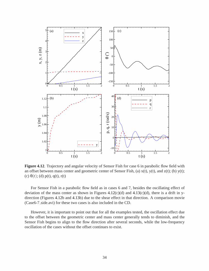
Figure 4.12. Trajectory and angular velocity of Sensor Fish for case 6 inparabolic flow field withan offset between mass center and geometric center of SensorFish, (a) x(t), y(t), and z(t); (b) y(t);(c) θ(t); (d) p(t), q(t), r(t)
For Sensor Fish in a parabolic flow field as in cases 6 and 7, besides the oscillating effect ofdeviation of the mass center as shown in Figures4.12(c)(d) and4.13(c)(d), there is a drift in y-direction (Figures4.12b and4.13b) due to the shear effect in that direction. A comparison movie(Case6-7side.avi) for these two cases is also included in the CD.
However, it is important to point out that for all the examples tested, the oscillation effect dueto the offset between the geometric center and mass center generally tends to diminish, and theSensor Fish begins to align to the flow direction after several seconds, while the low-frequencyoscillation of the cases without the offset continues to exist.
34

t (s)
x,y,
z(m
)
0 0.5 1 1.5 20
1
2
3
4
5xyz
(a)
t (s)
θ(o )
0 0.5 1 1.5 2
-150
-100
-50
0
50
100
150 (c)
t (s)
p,q,
r(r
ad/s
)
0 0.5 1 1.5 2
-10
0
10
20
30
40
pqr
(d)
t (s)
y(m
)
0 0.5 1 1.5 2
0.94
0.96
0.98
1
1.02
y
(b)
Figure 4.13. Trajectory and angular velocity of Sensor Fish for case 7 inparabolic flow field withmass center and geometric center of Sensor Fish overlapped,(a) x(t), y(t), and z(t); (b) y(t); (c)θ(t); (d) p(t), q(t), r(t)
35

5.0 Summary
As part of the process of redesigning the current 3DOF SensorFish device rate gyros will beadded to the new six degree of freedom (6DOF) device to measure each of the six linear and angularaccelerations. However, before the 6DOF Sensor Fish devicecan be developed and deployed,governing equations of motion must be developed in order to understand the design implicationsof instrument selection and placement within the body of thedevice.
As part of the initial steps in the design process, this report developed a fairly general formu-lation for the coordinate systems, equations of motion, force and moment relationships necessaryto simulate the the 6DOF movement of an underwater body. Somesimplifications are made byconsidering the Sensor Fish device to be a rigid, axisymmetric body. The equations of motion arewritten in the body-fixed frame of reference. Transformations between the body-fixed and iner-tial reference frames are performed using a formulation based on quaternions. Force and momentrelationships specific to the Sensor Fish body are currentlynot available. However, examples ofthe trajectory simulations using the 6DOF equations are presented using existing low and high-Reynolds number force and moment correlations. Animation files for the test cases are providedin an attached CD.
The next phase of the work will focus on the refinement and application of the 6DOF simulatordeveloped in this project. Experimental and computationalstudies are planned to develop a set offorce and moment relationships that are specific to the Sensor Fish body over the range of Reyn-olds numbers that it experiences. Lab testing of prototype 6DOF Sensor Fish will also allow forrefinement of the trajectory simulations through comparison with observations in test flumes. The6DOF simulator will also be an essential component in tools to analyze field data measured usingthe next generation Sensor Fish. The 6DOF simulator will be embedded in a moving-machinerycomputational fluid dynamics (CFD) model for hydroturbines to numerically simulate the 6DOFSensor Fish.
37

6.0 References
Batchelor GK. 1967.An Introduction to Fluid Dynamics. Cambridge University Press, Cam-bridge, United Kingdom.
Becker JM, CS Abernethy, and DD Dauble. 2003. “Identifying theEffects on Fish of Changes inWater Pressure During Turbine Passage.”Hydro Review5:32–42.
Blevins RD. 1993.Formulas for Natural Frequency and Mode Shape. Krieger Publishing Com-pany, Melbourne, Florida.
Broday D, M Fichman, M Shapiro, and C Gutfinger. 1998. “Motion of Spheroidal Particles inVertical Shear Flows.”Physics of Fluids10:86–100.
Carlson TJ. 2001.Proceedings of the Turbine Passage Survival Workshop, Portland, Oregon.PNNL-SA-33996, Pacific Northwest National Laboratory, Richland, Washington.
Carlson TJ and JP Duncan. 2003.Evolution of the Sensor Fish Device for Measuring PhysicalConditions in Severe Hydraulic Environments. DOE/ID-11079, U.S. Department of Energy IdahoOperations Office, Idaho Falls, Idaho.
Carlson TJ, JP Duncan, and TL Gilbride. 2003. “The Sensor Fish: Measuring Fish Passage inSevere Hydraulic Conditions.”Hydro ReviewXXII:62–69.
Cada GF. 1998. “Better Science Supports Fish-Friendly Turbine Designs.” Hydro ReviewXVII:52–61.
Cada GF. 2001. “The Development of Advanced Hydroelectirc Turbines to Improve Fish PassageSurvival.” Fishery26:14–23.
Conte G and A Serrani. 1996. “Modelling and Simulation of Underwater Vehicles.” InProceed-ings of the 1996 IEEE International Symmposium on Computer-Aided Control System Design,pp. 61–67. IEEE, Dearborn, Michigan.
Feng J and DD Josepth. 1995. “The Unsteady Motion of Solid Bodies in Creeping Flow.”Journalof Fluid Mechanics303:83–102.
Fossen TI. 1994.Guidance and Control of Ocean Vehicles. John Wiley & Sons, New York.
Happel J and H Brenner. 1983.Low Reynolds Number Hydrodynamics. Kluwer, Boston.
Harper EY and ID Chang. 1968. “Maximum Dissipation Resulting from Lift in a Slow ViscousShear Flow.”Journal of Fluid Mechanics33:209–225.
Hoerner SF. 1965.Fluid Dynamics Drag. Hoerner Fluid Dynamics, Brick Town, New Jersey.
Hoerner SF. 1985.Fluid Dynamics Lift. Hoerner Fluid Dynamics, Brick Town, New Jersey.
39

Hughes PC. 1986.Spacecraft Attitude Dynamics. John Wiley & Sons, New York.
Jeffery GB. 1922. “The Motion of Ellipsoid Particles Immersed in a Viscous Fluid.”Proceedingsof Royal Society102:161–179.
Maxey MR and JJ Riley. 1983. “Equation of Motion for a Small Rigid Sphere in a NonuniformFlow.” Physics of Fluids26:883–889.
Mougin G and J Magnaudet. 2002. “The Generalized Kirchhoff Equations and their Applica-tion to the Interaction Between a Rigid Body and an Arbitrary Time-Dependent Viscous Flow.”International Journal of Multiphase Flow28:1837–1851.
Munson BR, DF Young, and TH Okiishi. 1999.Fundamentals of Fluid Mechanics. John Wiley& Sons, New York.
Newman JN. 1977.Marine Hydrodynamics. MIT Press, Cambridge, Massachusetts.
Nietzel DA, MC Richmond, DD Dauble, RP Mueller, RA Moursund, CS Abernethy, GR Guen-sch, and GFCada. 2000.Laboratory Studies on the Effects of Shear on Fish: Final Report.DOE/ID-10822, U.S. Department of Energy Idaho Operations Office, Idaho Falls, Idaho.
Prestero T. 2001. “Verification of a Six-Degree of Freedom Simulation Model for the REMUSAutonomous Underwater Vehicle.” Master’s thesis, Massachusetts Institute of Technology, Cam-bridge, Massachusetts.
Richmond MC, TJ Carlson, JA Serkowski, CB Cook, and JP Duncan. 2004. “Characterizing theFish-Passage Environment at The Dalles Dam Spillway.” In2004 World Water and EnvironmentalResouces Congress. Salt Lake City, Utah.
Saffman PG. 1965. “The Lift on a Small Sphere in a Slow Shear Flow.” Journal of Fluid Mechan-ics 22:385–400.
Shi L, JM Doster, and CW Mayo. 1999. “Drag Coefficient for ReactorLoose Parts.”NuclearTechnology127:24–37.
Wertz JR. 1985.Spacecraft Attitude Determination and Control. D. Reidel Publishing Company,Boston.
Zhang H, G Ahmadi, F Fan, and JB McLaughlin. 2001. “Ellipsoidal Particles Transport andDeposition in Turbulent Channel Flows.”International Journal of Multiphase Flow27:971–1009.
40

Appendix A
Ellipsoid Motion Equations for Low ReynoldsNumbers

Appendix A: Ellipsoid Motion Equations for Low ReynoldsNumbers
Zhang et al. (2001) derived equations of motion for an ellipsoidal particle entrained in turbu-lent channel flows. The slip velocity is assumed sufficientlysmall so that the forces and torques(moments) acting on the body are obtained from the expressions for the low-Reynolds number orcreeping flow regime. In this flow regime, the hydrodynamic drag and shear-induced lift tend tobe directly proportional (linearly) to the slip velocity. They wrote the translational equations ofmotion, i.e., Newton’s law ofF = ma, in the inertial reference frame. However, the equations forrotational motion were given in terms of the body-fixed framewith angular velocity componentsaround this frame.
In the formulation of the motion equations presented in thisreport, all the forces and momentsare expressed in the body-fixed frame. To be consistent, we adapt the formulation of Zhang et al.(2001) accordingly. In addition, in this Appendix, the semi-major axis is Z-axis instead of X-axisas in the main report.
Recall that the flow field has (Vx, Vy, Vz) in the inertial frame and (V1, V2, V3) in the body-fixedframe as discussed in Chapter3.1(Page11), then in the body-fixed frame, the drag force becomes
FD = µπaK ·
V1−uV2−vV3−w
(A.1)
where a is the semi-minor axis of the ellipsoid of revolutionand
K =
kx 0 00 ky 00 0 kz
(A.2)
is called the translation dyadic. For the ellipsoid rotatedaround the Z-axis, it is determined byβ = b/a (ratio of semi-major axis to semi-minor axis)
kx = ky =16(β2−1)
(2β2−3)ln(β+
√(β2−1))√
(β2−1)+β
(A.3)
kz =8(β2−1)
(2β2−1)ln(β+
√(β2−1))√
(β2−1)−β
(A.4)
Note that the semi-major axis is aligned along the body-fixedZ-axis and
Q−1 ·K ·Q
A.1

is the dyadic in the inertial frame.
The shear-induced lift force for an arbitrary-shaped particle was obtained by Harper and Chang(1968) and the equation for it was re-stated by Zhang et al. (2001).
In the body-fixed frame, the lift force is
FL =µπ2a2√
ν·√
∣
∣
∣
∣
∂Vx
∂y
∣
∣
∣
∣
·S′x · (K ·D′
x ·K) ·
V1−uV2−vV3−w
(A.5)
whereD′
x = Q ·Dx ·Q−1 (A.6)
with
Dx =
0.0501 0.0329 00.0182 0.0173 0
0 0 0.0373
(A.7)
being a special matrix that remains fixed, and
S′x = Q ·Sx ·Q−1 (A.8)
with
Sx =
1 0 0
0 sign(
∂Vx∂y
)
0
0 0 1
(A.9)
This force applies only for a flow field in the x-direction withshear in only the orthogonaly-direction. For flow in the y-direction as well, with shear in the x-direction, a similar additionalforce would likely need to be superimposed. Then arrangement of elements inSx would need tobe changed to describe the orthogonal shear direction.
In particular, to find shear-lift in the orthogonal direction replaceDx by Dy given below andreplace the x-component flow velocity gradient with respectto y by the y-component velocitygradient with respect to x
D′y = Q ·Dy ·Q−1 (A.10)
and
Dy =
0.0173 0.0182 00.0329 0.0501 0
0 0 0.0373
(A.11)
Thus the orthogonal lift is
FL =µπ2a2√
ν·√
∣
∣
∣
∣
∂Vy
∂x
∣
∣
∣
∣
·S′y · (K ·D′
y ·K) ·
V1−uV2−vV3−w
(A.12)
A.2

whereS′
y = Q ·Sy ·Q−1 (A.13)
and
Sy =
sign(
∂Vy∂x
)
0 0
0 1 00 0 1
(A.14)
In general, the two force expressions for shear-lift are added together when flow is neither en-tirely in the x or y directions. In this trajectory model, shear in the vertical z-direction is presumednot to occur, or is presumed minor.
Zhang et al. (2001) pointed out that Jeffery (1922) originally derived the torque on an ellip-soid in a flow field having deformation and angular velocity (vorticity). To express the torquecomponents, it is necessary to calculate the flow velocity gradients in the body-fixed frame,
∇Vb = Q · (∇Ve) ·Q−1 and ∇Ve =
∂Vx∂x
∂Vx∂y
∂Vx∂z
∂Vy∂x
∂Vy∂y
∂Vy∂z
∂Vz∂x
∂Vz∂y
∂Vz∂z
(A.15)
where the subscripts b and e relate to the body-fixed frame andthe earth-fixed (inertial) frame,respectively.
The deformation rate and vorticity are
γ32 =12
[(∇Vb)3,2 +(∇Vb)2,3)] , γ13 = 12 [(∇Vb)1,3 +(∇Vb)3,1)] , (A.16)
ω1 =12
[(∇Vb)3,2− (∇Vb)2,3)] , ω2 = 12 [(∇Vb)1,3− (∇Vb)3,1)] , ω3 =
12
[(∇Vb)2,1− (∇Vb)1,2)] .
Notice that the vorticity in the body-fixed frame is the transformation of the same quantity in theinertial frame, as described in equation3.5(Page11).
The torque components are now given in the body-fixed frame by
∑MX =16πµa3β
3(βo +β2γo)
[
(1−β2)γ32+(1+β2)(ω1− p)]
∑MY =16πµa3β
3(βo +β2γo)
[
(β2−1)γ13+(1+β2)(ω2−q)]
(A.17)
∑MZ =32πµa3β3(βo +αo)
(ω3− r)
where
αo = βo =β2
β2−1+
β2(β2−1)3/2
ln
(
β−√
β2−1
β+√
β2−1
)
(A.18)
γo =−2
β2−1− β
2(β2−1)3/2ln
(
β−√
β2−1
β+√
β2−1
)
(A.19)
A.3

The trajectory equations for rotation assumed by Zhang et al. (2001) require the ellipsoidcenter of buoyancy and center of mass to coincide. In terms ofthe angular velocities, the equationsof rotational velocities are
Ixxp+(Izz− Iyy)qr = ∑MX
Iyyq+(Ixx− Izz)pr = ∑MY (A.20)
Izzr +(Iyy− Ixx)pq= ∑MZ
where moments of inertia are given for an ellipsoid as
m=43
πa3βρo, Ixx = Iyy =(1+β2)a2
5m, Izz=
2a2
5m (A.21)
In the context of the more general situation when center of mass is not located at the center ofthe ellipsoid. Let(0, 0, zg) indicate the location of center of mass relative to the ellipsoid center,the rotation would be expressed by the following
Ixxp+(Izz− Iyy)qr−mzg(v−wq+ur) = ∑MX −zgWQ2,3
Iyyq+(Ixx− Izz)pr +mzg(u−vr +wq) = ∑MY +zgWQ1,3 (A.22)
Izzr +(Iyy− Ixx)pq = ∑MZ
whereW is the weight of the particle. Note that moment of inertial need to be re-calculated due tothe offset of geometric center and mass center.
The final equations for simulation of an ellipsoidal particle are obtained by substituting equa-tions A.2, A.5, andA.12 into the equations of translational motion, and including the equationsof rotational motion (equationA.22 and the properties of quaternion representation (equations 4.5and4.7).
A.4

Appendix B
Nomenclature

Appendix B: Nomenclature
The following is a list of the symbols and their definitions used in this document. As a commonpractice, symbols in bold face are defined as vectors or tensors, and symbols dotted above are timederivative in their own coordinate systems.
A Homogeneous transform matrix given aset of roll, pitch, and yaw angles
Ai, j components of transform matrixA,i, j = 1,2,3
Af Frontal area of Sensor Fish,π(d/2)2
Ap Projected area of Sensor Fish,πdL
B Magnitude of buoyancy
C 6×6 matrix of coefficient on the left sideof 6DOF motion equations
CD axial drag coefficient
FA Resultant of forces due to added mass inbody-fixed frame
FD Resultant of drag forces in body-fixedframe
FHS Resultant of hydrostatic forces inbody-fixed frame
FL Resultant of lift forces in body-fixedframe
H Inverse of coefficient matrix C,C−1
I Inertial tensor of a rigid body
Ii j Components of inertial tensor inbody-fixed frame,i, j = x,y,z
I ′ Normalized inertial tensor of a rigidbody,I/m
I ′i j Components of normalized inertial tensorin body-fixed frame,I ′i j = Ii j /m, i, j = x,y,z
J Transform matrix for rotational velocitiesgiven a set of roll, pitch, and yaw angles
KA Resultant of moments due to added massalong body-fixed X-axis
KAp Coefficients of moments due to addedmass in body-fixed frame
KD Resultant of drag moments alongbody-fixed X-axis
KDww Drag moment coefficient in body-fixedframe
KHS Resultant of hydrostatic moments alongbody-fixed X-axis
KL Resultant of lift moments alongbody-fixed X-axis
L Length of Sensor Fish
MA Resultant of moments due to added massin body-fixed frame
MA Resultant of moments due to added massalong body-fixed Y-axis
MAi Coefficients of moments due to addedmass in body-fixed frame,i = w, q,uw,vp, rp,uq
MD Resultant of drag moments in body-fixedframe
MD Resultant of drag moments alongbody-fixed Y-axis
MDww Drag moment coefficient in body-fixed
B.1

frame
MDqq Drag moment coefficient in body-fixedframe
MHS Resultant of hydrostatic moments inbody-fixed frame
MHS Resultant of hydrostatic moments alongbody-fixed Y-axis
ML Resultant of lift moments in body-fixedframe
ML Resultant of lift moments alongbody-fixed Y-axis
MLuw Lift moment coefficient along body-fixedY-axis
NA Resultant of moments due to added massalong body-fixed Z-axis
NAi Coefficients of moments due to addedmass in body-fixed frame,i = v, r,uv,wp, pq,ur
ND Resultant of drag moments alongbody-fixed Z-axis
NDvv Drag moment coefficient in body-fixedframe
NDrr Drag moment coefficient in body-fixedframe
NHS Resultant of hydrostatic moments alongbody-fixed Z-axis
NL Resultant of lift moments alongbody-fixed Z-axis
NLuv Lift moment coefficient along body-fixedZ-axis
Q Transformation matrix in terms ofquaternion components
Qi, j Components of transform matrixQ,i, j = 1,2,3
Re Reynolds number based on slip velocity
of Sensor Fish,UslipL/ν
Ti Non-acceleration terms defined inEquation4.2, i = 1,2,3
Uslip Slip velocity of Sensor Fish
V1 Axial velocity (X-axis) of ambient flowfield in body-fixed frame
V1 Axial acceleration (X-axis) of ambientflow field in body-fixed frame,dV1
dt
V2 Spanwise velocity (Y-axis) of ambientflow field in body-fixed frame
V2 Spanwise acceleration (Y-axis) ofambient flow field in body-fixed frame,dV2dt
V3 Vertical velocity (Z-axis) of ambient flowfield in body-fixed frame
V3 Vertical acceleration (Z-axis) of ambientflow field in body-fixed frame,dV3
dt
Vx Axial velocity (x-axis) of ambient flowfield in inertial frame
Vx Axial acceleration (x-axis) of ambientflow field in inertial frame,dVx
dt
Vy Spanwise velocity (y-axis) of ambientflow field in inertial frame
Vy Spanwise acceleration (y-axis) of
ambient flow field in inertial frame,dVydt
Vz Vertical velocity (z-axis) of ambient flowfield in inertial frame
Vz Vertical acceleration (z-axis) of ambientflow field in inertial frame,dVz
dt
W Weight of Sensor Fish
XA Resultant of forces due to added massalong body-fixed X-axis
XAi Coefficients of forces due to added massin body-fixed frame,i = u,wq,qq,vr, rr
B.2
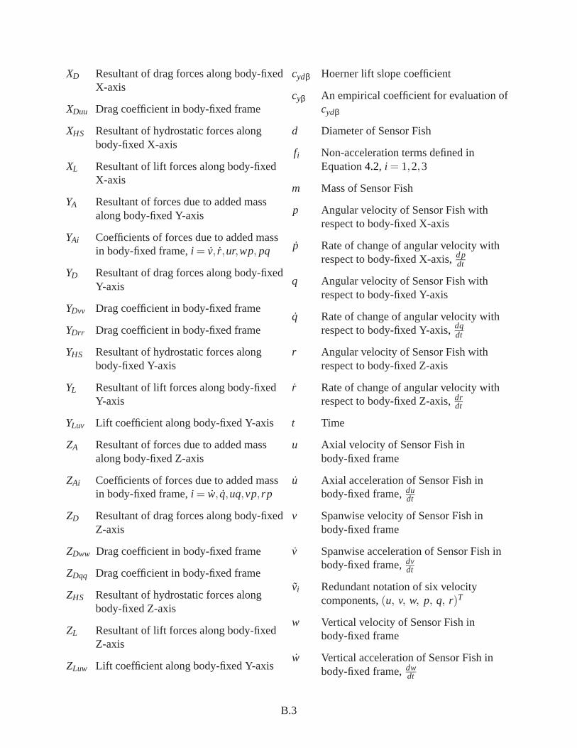
XD Resultant of drag forces along body-fixedX-axis
XDuu Drag coefficient in body-fixed frame
XHS Resultant of hydrostatic forces alongbody-fixed X-axis
XL Resultant of lift forces along body-fixedX-axis
YA Resultant of forces due to added massalong body-fixed Y-axis
YAi Coefficients of forces due to added massin body-fixed frame,i = v, r,ur,wp, pq
YD Resultant of drag forces along body-fixedY-axis
YDvv Drag coefficient in body-fixed frame
YDrr Drag coefficient in body-fixed frame
YHS Resultant of hydrostatic forces alongbody-fixed Y-axis
YL Resultant of lift forces along body-fixedY-axis
YLuv Lift coefficient along body-fixed Y-axis
ZA Resultant of forces due to added massalong body-fixed Z-axis
ZAi Coefficients of forces due to added massin body-fixed frame,i = w, q,uq,vp, rp
ZD Resultant of drag forces along body-fixedZ-axis
ZDww Drag coefficient in body-fixed frame
ZDqq Drag coefficient in body-fixed frame
ZHS Resultant of hydrostatic forces alongbody-fixed Z-axis
ZL Resultant of lift forces along body-fixedZ-axis
ZLuw Lift coefficient along body-fixed Y-axis
cydβ Hoerner lift slope coefficient
cyβ An empirical coefficient for evaluation ofcydβ
d Diameter of Sensor Fish
fi Non-acceleration terms defined inEquation4.2, i = 1,2,3
m Mass of Sensor Fish
p Angular velocity of Sensor Fish withrespect to body-fixed X-axis
p Rate of change of angular velocity withrespect to body-fixed X-axis,dp
dt
q Angular velocity of Sensor Fish withrespect to body-fixed Y-axis
q Rate of change of angular velocity withrespect to body-fixed Y-axis,dq
dt
r Angular velocity of Sensor Fish withrespect to body-fixed Z-axis
r Rate of change of angular velocity withrespect to body-fixed Z-axis,dr
dt
t Time
u Axial velocity of Sensor Fish inbody-fixed frame
u Axial acceleration of Sensor Fish inbody-fixed frame,du
dt
v Spanwise velocity of Sensor Fish inbody-fixed frame
v Spanwise acceleration of Sensor Fish inbody-fixed frame,dv
dt
vi Redundant notation of six velocitycomponents,(u, v, w, p, q, r)T
w Vertical velocity of Sensor Fish inbody-fixed frame
w Vertical acceleration of Sensor Fish inbody-fixed frame,dw
dt
B.3

x Axial position of Sensor Fish withrespect to inertial frame
x Axial velocity of Sensor Fish in inertialframe,dx
dt
xb Axial position of center of buoyancy inbody-fixed frame
xcp Location of resultant lift in body-fixedframe
xg Axial position of center of mass inbody-fixed frame
y Spanwise position of Sensor Fish withrespect to inertial frame
y Spanwise velocity of Sensor Fish ininertial frame,dy
dt
yb Spanwise position of center of buoyancyin body-fixed frame
yg Spanwise position of center of mass inbody-fixed frame
z Vertical position of Sensor Fish withrespect to inertial frame
z Vertical velocity of Sensor Fish in inertialframe,dz
dt
zb Vertical position of center of buoyancy inbody-fixed frame
zg Vertical position of center of mass inbody-fixed frame
ε Quaternion,(ε1,ε2,ε3,ε4)T
ε1 First component of quaternionε
ε2 Second component of quaternionε
ε3 Third component of quaternionε
ε4 Fourth component of quaternionε
θ Pitch angle of Sensor Fish with respect toinertial frame
θ Angular velocity of Sensor Fish with
respect to inertial y-axis,dθdt
ν Kinematic viscosity of water
ρ Density of water
ρo Density of Sensor Fish or the underwaterrigid-body
φ Roll angle of Sensor Fish with respect toinertial frame
φ Angular velocity of Sensor Fish withrespect to inertial x-axis,dφ
dt
ψ Yaw angle of Sensor Fish with respect toinertial frame
ψ Angular velocity of Sensor Fish withrespect to inertial z-axis,dψ
dt
Ω Angular velocity vector of Sensor Fishwith respect to body-fixed frame,(p, q, r)T
ω1 Angular velocity of ambient flow withrespect to body-fixed X-axis
ω1 Rate of change of ambient flow angularvelocity with respect to body-fixedX-axis, dω1
dt
ω2 Angular velocity of ambient flow withrespect to body-fixed Y-axis
ω2 Rate of change of ambient flow angularvelocity with respect to body-fixedY-axis, dω2
dt
ω3 Angular velocity of ambient flow withrespect to body-fixed Z-axis
ω3 Rate of change of ambient flow angularvelocity with respect to body-fixedZ-axis, dω3
dt
ωx Angular velocity of ambient flow withrespect to inertial x-axis
ωx Rate of change of ambient flow angularvelocity with respect to inertial x-axis,
B.4

dωxdt
ωy Angular velocity of ambient flow withrespect to inertial y-axis
ωy Rate of change of ambient flow angularvelocity with respect to inertial y-axis,dωydt
ωz Angular velocity of ambient flow withrespect to inertial z-axis
ωz Rate of change of ambient flow angularvelocity with respect to inertial z-axis,dωzdt
∇Vb Gradient tensor of ambient flow velocityin body-fixed frame
∇Ve Gradient tensor of ambient flow velocityin inertial frame
∑F Resultant of external forces in body-fixedframe
∑FX Resultant of external forces alongbody-fixed X-axis
∑F ′X Normalized resultant of external forces
along body-fixed X-axis,∑FX/m
∑FY Resultant of external forces alongbody-fixed Y-axis
∑F ′Y Normalized resultant of external forces
along body-fixed Y-axis,∑FY/m
∑FZ Resultant of external forces alongbody-fixed Z-axis
∑F ′Z Normalized resultant of external forces
along body-fixed Z-axis,∑FZ/m
∑M Resultant of external moments inbody-fixed frame
∑MX Resultant of external forces with respectto body-fixed X-axis
∑M′X Normalized resultant of external
moments with respect to body-fixedX-axis,∑MX/m
∑MY Resultant of external forces with respectto body-fixed Y-axis
∑M′X Normalized resultant of external
moments with respect to body-fixedY-axis,∑MY/m
∑MZ Resultant of external forces with respectto body-fixed Z-axis
∑M′Z Normalized resultant of external
moments with respect to body-fixedZ-axis,∑MZ/m
B.5