DISCLAIMER: © Copyright: 2014

DISCLAIMER: This publication is intended for EDUCATIONAL purposes only. The information contained herein is subject to change with no notice, and while a great deal of care has been taken to provide accurate and current information, UBC, their affiliates, authors, editors and staff (collectively, the "UBC Group") makes no claims, representations, or warranties as to accuracy, completeness, usefulness or adequacy of any of the information contained herein. Under no circumstances shall the UBC Group be liable for any losses or damages whatsoever, whether in contract, tort or otherwise, from the use of, or reliance on, the information contained herein. Further, the general principles and conclusions presented in this text are subject to local, provincial, and federal laws and regulations, court cases, and any revisions of the same. This publication is sold for educational purposes only and is not intended to provide, and does not constitute, legal, accounting, or other professional advice. Professional advice should be consulted regarding every specific circumstance before acting on the information presented in these materials. © Copyright: 2014 by the UBC Real Estate Division, Sauder School of Business, The University of British Columbia. Printed in Canada. ALL RIGHTS RESERVED. No part of this work covered by the copyright hereon may be reproduced, transcribed, modified, distributed, republished, or used in any form or by any means – graphic, electronic, or mechanical, including photocopying, recording, taping, web distribution, or used in any information storage and retrieval system – without the prior written permission of the publisher.

LESSON 1

Introduction to Excel – Orientation and Tools

Assigned Reading 1. UBC Real Estate Division. 2014. CPD 152 Financial Analysis with Excel. Vancouver: UBC Real Estate

Division. Lesson 1: Introduction to Excel: Orientation and Tools 2. UBC Real Estate Division. "Introduction to Excel – Screencast Video Series". A series of 14 videos

between 9 and 22 minutes long, providing orientation and instruction on how to use Excel. Sessions 1-6, 9, 10, 14: Orientation, formatting, basic functions Sessions 12-13: Financial calculations

Recommended Reading 1. Excel Tutorials:

• Microsoft: Various tutorials ranging from easy to advanced for Excel 2007, 2010, 2013, and Excel for Mac 2011.

• Learnfree.org: Provides quite basic instructions for various versions of Excel (2002, 2007, 2010, etc.) Explains the basics with screenshots and video tutorials. Some lessons include cell basics, creating complex formulas, formatting, and creating tables.

• SSC-Stat: Excel Add-in webpage. A free add-on for Excel, to allow much more in-depth statistical and graphical analysis capabilities.

• UBC Real Estate Division. "Introduction to Excel – Screencast Video Series". A series of 14 videos between 9 and 22 minutes long, providing orientation and instruction on how to use Excel. Sessions 7-8, 11: Statistical operations

Learning Objectives

After completing this lesson, the student should be able to:

1. identify and define the components of an Excel spreadsheet; 2. explain the basic types of data in an Excel spreadsheet; 3. calculate basic mathematical operations using Excel; 4. review the library of pre-programmed functions in Excel and insert a function using the specified inputs;

calculate common non-financial functions in Excel, such as sum, average, maximum, minimum, if, what if, and goal seek;

5. calculate the following financial functions in Excel: present value, future value, equivalent interest rates, payment, rate, amortization, outstanding balance, principal interest split, net present value, and internal rate of return;

6. copy and paste formulas with absolute and relative positioning; 7. work with multiple tabs and worksheets; and 8. hide and freeze columns and rows in an Excel spreadsheet.

Note: All readings can be found under Lesson 1 and Software Help on your course website

1.1

https://secure.sauder.ubc.ca/re_creditprogram/course_resources/courses/content/344/presentations/excelintro.cfm?cr_view=%23cr_view%23

http://www.reading.ac.uk/ssc/n/n_sscstat.htm

https://secure.sauder.ubc.ca/re_creditprogram/course_resources/courses/content/344/presentations/excelintro.cfm?cr_view=%23cr_view%23

Lesson 1

Instructor's Comments This lesson provides an introduction to the Microsoft Excel spreadsheet program. This is an indispensable tool in contemporary business practice. The goal of this lesson will be to provide orientation to the program and outline basic tools and functions. In Lesson 2, we will advance to look at case studies of specific applications for spreadsheets. It is strongly recommended that you have Excel running while you work through this lesson, as the best way to learn the tools and functions that Excel has to offer. You will find a series of "screen-cast" videos on the course website. These are an excellent learning resource that you should check out. They cover the basics of using Excel as well as more advanced financial and statistical functions. Introduction to Spreadsheets

A spreadsheet is the computer equivalent of a paper ledger sheet. It consists of a grid made from columns and rows. It is an environment that can make number manipulation easy and less painful.

The math that goes on behind the scenes on the paper ledger can be overwhelming. If you change the loan amount, you will have to start the math all over again. But let's take a closer look at the computer version. The previous two ledgers seem pretty evenly matched. Right? Wrong! The nice thing about using a computer spreadsheet is that you can experiment with numbers without having to re-do all the calculations. Let's change the interest rate and then the number of months. Let the computer do the calculations! Once we have the formulas set up, we can change the variables that are used in the formula and watch the changes. Change the Interest Rate Change the Number of Months

Much of this introductory material has been reprinted, with permission, from the Excel Tutorial on the TRIO program webpage of the University of South Dakota.

1.2


If you are doing this on paper, you will have to get your calculator back out, grab an eraser and hope you punched all the right keys and in the right order. A benefit of spreadsheets is that calculations are instantly updated if one of the referenced entries is changed. Furthermore, it is much easier to track down errors using a computer spreadsheet as the data is all stored in front you at one time. Spreadsheets can be very valuable tools in business. They are often used to play out a series of what-if scenarios (much like our car purchase here). Spreadsheet Components So let's get started digging into what makes a spreadsheet work. Spreadsheets are made up of:

• Columns • Rows • Cells (the intersections of columns and rows)

In each cell there may be the following types of information:

• Text labels: used to describe data • Number data (constants): used in calculations • Formulas: mathematical equations that utilize data to produce results

In a spreadsheet the column is defined as the vertical space that is going up and down the window. Letters are used to designate each column's location.

In the above diagram Column C is highlighted. The row is defined as the horizontal space that is going across the window. Numbers are used to designate each row's location.

1.3

Lesson 1

In the above diagram Row 4 is highlighted. The cell is defined as the space where a specified row and column intersect. Each cell is assigned a name according to its column letter and row number.

In the above diagram Cell B6 is highlighted. When referencing a cell, you should put the column first and the row second. In Excel there are limits to the number of rows and columns in a sheet…these limits in Excel 2013 are 16,384 columns and 1,048,576 rows. Columns are named from A to Z, then AA, AB, AC,…, to AZ, BA, BB,…,to ZZ, then AAA, AAB,… , to XFD. So the top leftmost cell is named A1 and the bottom rightmost cell (should you have that much data) is named XFD1048576. That is 17,179,869,184 cells (234).

1.4


Types of Data There are three basic types of data that can be entered in a spreadsheet:

• Labels (text with no numerical value) • Constants (just a number – constant value) • Formulas1 (a mathematical equation used to calculate)

Data types Examples Descriptions

LABEL NAME or WAGE or DAYS anything that is just text (could be any combination of alphanumeric characters usually used for titles or headings)

CONSTANT 5 or 3.75 or -7.4 any number

FORMULA =5+3 or =8*5+3 mathematical expression – must begin with an equal sign (=)

Labels are text entries. They do not have a value associated with them. We typically use labels to identify what we are talking about. In our first example, the labels were:

• computer ledger • car loan • interest • number of payments • monthly payment

Constants are entries that have a specific fixed value. If someone asks you how old you are, you would answer with a specific answer. Sure, other people will have different answers, but it is a fixed value for each person. In our first example, the constants were:

• $12,000 • 9.6% • 60

1 ALL formulas MUST begin with an equal sign (=).

1.5

Lesson 1

As you can see from these examples there may be different types of numbers. Sometimes constants are referring to dollars, sometimes referring to percentages, and other times referring to a number of items (in this case 60 months). These are typed into the spreadsheet with just the numbers and are changed to display their type of number by formatting (we will talk about this later). Formulas are entries that have an equation that calculates the value to display. We do not type in the numbers we are looking for; we type in the equation. The results of the equation will be updated upon the change or entry of any data that is referenced in the equation. When we are entering formulas into a spreadsheet we want to make as many references as possible to existing data. If we can reference that information we don't have to type it in again. More importantly, if that other information changes, we do not have to change the equations. For example, if you work for 23 hours and make $5.36 an hour, how much do you make? We can set up this situation using:

• Three labels • Two constants • One equation

Let's look at what could be in cell B4: =B1*B2 =23*5.36 $123.28

All three of these choices will produce the same answer, but one is much more useful than the other two. It is best if we can reference as much data as possible as opposed to typing in the answer or typing data into equations. In our last example, things were pretty straightforward. We had number of hours worked multiplied by wage per hour and we got our total pay. Once you have a working spreadsheet you can save your work and use it at a later time. If we referenced the actual cells, instead of typing in the answer or data into the equation, we could update the entire spreadsheet by just typing in the new hours worked.

Let's look at the new spreadsheet:

• Hours have been changed to 34 • Wage per hour is the same • Total Pay would have to be changed to either =34*5.36 or $182.24 • However, the formula would still be =B1*B2

If in cell B4 we had typed in either =23*5.36 or $123.28 the first time and just changed the hours worked here, Total Pay in cell B4 would still be $123.28, and we would have to retype what is in cell B4. Instead, we typed in references to the data that we wanted to use in the equation.

1.6


We typed in =B1*B2. These are the locations of the data that we want to use in our equation so Excel recalculates the Total Pay with the new values. Again, it is best if we can reference as much data as possible as opposed to typing data into equations or answers into the cell. Excel Formulas (Functions) Spreadsheets have many math functions built into them. Of the most basic operations are the standard multiply, divide, add, and subtract. These operations follow the order of operations (just like algebra). Let's look at some examples. For these following examples, consider the following data:

Operation Symbol Constant Data Referenced Cells Answer

Multiplication * =5*6 =A1*B3 30

Division / =8/4 =A3/B2 2

Addition + =4+7 =B2+A2 11

Subtraction – =8–3 =A3–B1 5

Selecting Cells Selecting cells is a very important concept of a spreadsheet. We need to know how to reference the data in other parts of the spreadsheet in order to specify the range of numbers that should be included in a formula or a graph. When entering your selection you may use the keyboard or the mouse. We can select several cells together if we can specify a starting cell and a stopping cell. This will select all the cells within this specified block of cells. Using the same data as before, we will look at various selection methods.

1.7

Lesson 1

Referring to the table below, if we wanted to add up the group of cells in the "To Add Up" column, you would insert the respective cell range found in the "Type In" column into the SUM formula, either by typing or clicking: =SUM(Type In) OR =SUM(Click On)

To Add Up Type In Click On

A1, A2, A3 A1:A3 A1, with button down drag to A3

A1, B1 A1:B1 A1, with button down drag to B1

A1, B3 A1, B3 A1, type in comma, B3

A1, A2, B1, B2 A1:B2 A1, with button down drag to B2

All Cells A1:B3 A1, with button down drag to B3

Accessing all the Functions While it is possible to type in every function in the keyboard, in Excel there is a help tool for functions called the Insert Function which will initiate the Function Wizard. There are three ways to access the function wizard:

1. If you look at the Standard Toolbar, the function wizard icon looks like . Clicking on the icon will open the Insert Function window.

2. Go to the Formulas tab, then Insert Function. 3. When you type in the "=" sign in a cell in order to start a formula, a menu of the most recent

functions used is available on the left.

1.8


Click on the arrow pointing down in order to open the menu and choose the function you want to use. If the function that you need does not appear on the pull down menu, click on "More Functions..." and the Insert Function window will appear. The Insert Function window appears with the function categories in a drop-down text box near the top with choices (such as Most Recently Used, All, Financial, and Statistical) and the functions in each category listed in the window below. Upon choosing the function and clicking OK, Excel will open a new window (Function Arguments) where you will input the data or cells or range of cells needed to complete the function. Mini descriptions are available for each of the functions. It is often necessary for you to understand the functions in order to be able to figure out these descriptions. In the window below, many functions needed to complete a statistics project are listed. You can access all of these functions by choosing the "Statistical" category and looking for the function name in the menu. Make sure that you choose the appropriate function! Many of the functions look similar, but have different properties (example: STDEV, STDEVA, STDEVP, STDEVPA). Read the brief description at the bottom of the window. Most of the time, you will be using the first type of the function listed (i.e. STDEV not STDEVA, STDEVP, not STDEVPA).

Some statistical measures do not have a corresponding function. For example, to calculate the coefficient of variation you will need to use the Excel functions to calculate the mean and the standard deviation and then use the coefficient of variation formula to calculate the statistic. Common Functions SUM Probably the most popular function in any spreadsheet is the SUM function. The SUM function takes all of the values in each of the specified cells and totals their values. The syntax is:

=SUM(first value, second value, …)

In the first and second spots you can enter any of the following (constant, cell, range of cells).

• Blank cells will return a value of zero to be added to the total. • Text cells cannot be added to a number and will produce an error.

1.9

Lesson 1

Notice that in A4 there is a text entry. This has no numeric value and cannot be included in a total or it will result in an error.

Example Cells to SUM Answer

=sum(A1:A3) A1, A2, A3 150

=sum(A1:A3, 100) A1, A2, A3, 100 250

=sum(A1+A4) A1, A4 #VALUE!

=sum(A1:A2, A5) A1, A2, A5 75

AVERAGE (MEAN) The AVERAGE function finds the arithmetic mean of the specified data. This is found by adding all of the indicated cells together and dividing by the total number of cells. The syntax is as follows:

=AVERAGE(first value, second value, …)

Text fields and blank entries are not included in the calculations of the Average function.

Example Cells to AVERAGE Answer

=average(A1:A4) A1, A2, A3, A4 62.5

=average(A1:A4, 300) A1, A2, A3, A4, 300 110

=average(A1:A5) A1, A2, A3, A4, A5 62.5

=average(A1:A2, A4) A1, A2, A4 58.33

MAXIMUM The next function we will discuss is MAX (Maximum). This will return the greatest (maximum) value in the selected range of cells. The syntax is as follows:

=MAX(first value, second value, …)

Text fields and blank entries are not included in the calculations of the Max Function.

MINIMUM The next function we will discuss is MIN (Minimum). This will return the lowest (minimum) value in the selected range of cells. The syntax is as follows:

=MIN(first value, second value, …)

Example of Max Cells to look at Answer

=max(A1:A4) A1, A2, A3, A4 30

=max(A1:A4,100) A1, A2, A3, A4, 100 100

=max(A1,A3) A1, A3 30

=max(A1, A5) A1, A5 10

1.10


Text fields and blank entries are not included in the calculations of the MIN Function.

Notice that there is no Range function in Excel. To find out the range of a sample, simply subtract the maximum value from the minimum value of the sample (try to do it by typing in an equation that will reference your Max and Min cell values). IF FUNCTION The IF function returns one value if a condition you specify is TRUE, and another value if that condition is FALSE. The formula is formatted as follows: =IF(logical_test, [value if true], [value if false]). Any value or expression that can be evaluated as either TRUE of FALSE can be placed in the logical test section. The most common logical tests are greater than (>), less than (<), or equal (=).

WHAT-IF ANALYSIS (Note: Do not confuse with IF function) Excel allows you to perform a basic sensitivity analysis of a change in a variable. The What-If analysis is a built in function that allows you to see the effect of a change in a key variable on a given outcome. In this example we will be using an NPV formula and changing the discount rate to see the varying outcomes (changes in NPV).

1. Set up the project's cash flows at the top of the page. Make sure to carefully enter positive or negative cash flows in each cell of the timeline. In this example the reversion is the sale price of the project.

Example of Min Cells to look at Answer

=min(A1:A4) A1, A2, A3, A4 10

=min(A2:A3,100) A2, A3, 100 20

=min(A1,A3) A1, A3 10

=min(A1,A5) A1, A5 (displays the least number) 10

Examples of IF Cells to look at Answer

=IF(A1>100,"Over 100","Under 100") A1 Under 100

=IF(A2>100,"Over 100","Under 100") A2 Over 100

=IF(A3+A1>100,"Over 100","Under 100") A3, A1 Over 100

=IF(A4-A2>100,"Over 100","Under 100") A4, A2 Under 100

1.11

Lesson 1

2. Create a dedicated cell for the discount rate (B8).

• Enter your NPV formula – type the equal sign followed by NPV and the open bracket.

• Then select the cell in which you have the discount rate (B8) followed by a comma.

• Next select each of your cash flow cells starting with period one (B5). Separate each entry with a comma. Note that the cash flow at period 5 is actually the sum of the $1,000 cash flow (F5) and the $40,000 reversion price (G5). This is because both occur at the same point in time.

• Close the brackets after the final year's cash flow. • Add in the cash flow occurring at time zero (A5).

• Press the enter key. You will notice that the cell now contains the NPV of the cash flows using a discount rate of 0.075.

3. Now it is time to construct the What-If worksheet.

• Enter the desired discount rates in a column, these will be the different rates used to test the NPV. Make sure the first cell in the worksheet corresponds to the rate that you used for your initial NPV calculation.

• In the cell to the right of the first value (B12) you will need to set it equal to the NPV formula. Click on the cell (B12) and press the = key, then click on the cell that contains the NPV formula (B7) and press the enter key. It should appear as the figure below:

1.12


• Now select the range of discount rates and the range of NPV values that you want to fill. Do this by clicking and dragging the mouse from the top left value to the bottom right value you want to select.

• At the toolbar at the top of the page, navigate to the Data tab.

• Click on the What-If Analysis button and then on the Data Table option from the drop down menu.

• A dialogue box will pop up on the screen. In the "Column input cell" dialogue box enter the location of the cell that held the original discount rate used in the NPV formula. In our example it is B8. The value can be entered in two ways, either by manually typing in $B$8 in the dialog box or by clicking on the discount rate cell.

• Click on the OK button and the table will be filled with different NPV values/outcomes for each corresponding discount rate.

The result of our sensitivity analysis is displayed above. Changing any cash flow value will automatically update the table.

1.13

Lesson 1

GOAL SEEK FUNCTION Prior to using the Goal Seek function, it must be installed on your computer as shown below.

1. Start by clicking on the MS Office button, then clicking Excel Options. (Note that these instructions and screenshots are from Excel 2007. In Excel 2003: Tools. In Excel 2013: File/Options.)

2. Then click Add-Ins located in the left pane, and then in the Manage box, select Excel Add-ins, and press Go. In the new window, check the Analysis ToolPak box, then click OK. (Excel 2003: Add-Ins/Analysis ToolPak/OK. Excel 2013: Add-ins/Excel Add-ins/Analysis ToolPak/OK.)

1.14


3. Navigate to the Data tab, and click on What-if Analysis, and then Goal Seek. (Excel 2003: Tools/Goal Seek. Excel 2013: Data/What-if Analysis/Goal Seek)

4. To fully utilize Goal Seek, you must set Excel to allow for a circular reference because Goal Seek's iterative analysis creates a circular reference. Normally Excel will not permit a circular reference unless permission for this condition is set in the control panel for the software. To do this, click on the MS Office button, then Excel options. Under the Formula tab, ensure that the Enable iterative calculation box is checked. (Excel 2003: Tools/Options/Calculation/ Enable iterative calculations. Excel 2013: File/Options/Formulas/Enable iterative calculation.)

1.15

Lesson 1

Once Goal Seek is installed, the Goal Seek function of Excel allows for a variable to be changed until the different outcomes match a defined outcome. We will now use it to solve for an NPV of zero, also known as the IRR. We will continue from the last example of creating a What-If worksheet.

1. Navigate to the Data tab found on the toolbar at the top of the page.

2. Click on the What-If Analysis button and then on the Goal Seek option from the drop down menu.

3. A dialogue box will appear on the screen. Place the cursor in the "Set cell" dialogue box and click

on the cell containing the NPV formula (B7) as we discussed in the previous section. Enter a value of zero in the "To value" dialogue box. Place the cursor in the "By changing cell" dialogue box and select the cell containing the discount rate (B8).

4. Click OK and OK again. Excel will change the NPV to zero and a new discount rate will be

displayed.

In this example we used Goal Seek to find a discount rate that resulted in an NPV of zero. While some might notice that this can also be achieved by using Excel's IRR function, the Goal Seek function allows the user to look for any target NPV.

1.16


Financial Functions Excel has all of the common financial formulas programmed into its functions, making it quite simple to solve financial problems. These financial functions are the most important tool in Excel for many business users. While these problems can be solved using mathematical formulas or a financial calculator, the spreadsheet speeds this up. The spreadsheet allows for quick iterative "what if" analysis, where you can change an input and see how it affects the outcome – a cumbersome process with a calculator. As well, once programmed, a spreadsheet can be re-used in many different circumstances, compounding its benefits indefinitely. In this section, we will illustrate each of the main financial functions in Excel. Note that Excel offers many more financial functions beyond these – see the Functions menu in the program for a comprehensive listing and instructions on how to use them. Illustration 1.1 A commercial enterprise has arranged for an interest accrual loan whereby the $10,000 amount borrowed is to be repaid in full at the end of one year. The borrower has agreed, in addition, to pay interest at the rate of 8% per annum, compounded annually on borrowed funds and this interest is to be calculated and paid at the end of the loan's one-year term. Calculate the amount of interest due and the total amount owing at the end of the term of the loan.

Solution

To obtain the interest (I), enter =B4*B3*B5 where B4 is $10,000, B3 is 8%, and B5 is 1 year. To obtain the future value, enter =B4+B7 where B7 is the total interest (I).

Note: you can also state cell B4 (8%) as 0.08; however, if you include the percentage sign, Excel will automatically switch from a percentage to a decimal.

The Power of Spreadsheets

By using a spreadsheet like Excel, we can solve financial problems either by programming in math formulas manually or by the use of Excel's pre-programmed financial formulas. For this simple example in Illustration 1.1, we identify the loan amount (PV), interest rate, and loan period, and then calculate the amount of interest and future value amount. If we specify the numbers in separate cells, and then program the cell coordinates into the formulas, it allows us the flexibility to easily change a number and then recalculate the future value. For example, if we change the loan amount to $5,000, we change that one cell (B4) from $10,000 to $5,000. Then the interest amount will change to $400 and future value to $5,400. This is a simple example of the dynamic nature of spreadsheets – which can be very useful in working with highly complex, sophisticated analyses.

Full solutions of all illustrations and exercises are provided in this lesson and are also available under Lesson 1 on your course website.

1.17

Lesson 1

Present Value You can solve for the present value of interest accrual loans in Excel by either using the math formula or the pre-programmed financial function. Recall that the formula for the present value of interest accrual loans and investments is as follows:

PV = FV × (1 + jm/m)-n

where

jm = nominal (annual rate of interest-j-) with a stated compounding frequency (m) PV = Present value FV = Future value after n periods n = Number of compounding or payment periods in the financial problem

The present value pre-programmed function in Excel calculates the present value for a loan or investment given the periodic rate, the number of periods, and the future value. The pre-programmed function for present value is =PV(RATE, NPER, PMT, FV, TYPE) where:

• RATE represents the periodic interest rate for the loan or investment • NPER represents the total number of payments • PMT represents the payment made or received each period (zero in this case) • FV represents the future value • TYPE represents when the payments are due (0 at the end of the period or omitted, 1 at the

beginning of the period) To calculate the PV using the pre-programmed Excel function, perform the following steps:

• Select the Formulas tab, then click Insert Function • Select Financial from the drop-down list, scroll down, then double-click on PV • State the cell reference for each of the associated components • Select OK and the result will display in the formula cell

Interest Rates: Percent or Decimal

The HP10BII/II+ financial calculators require interest rates to be entered in percent form, not decimals, and as a rate per year (nominal rate). When using math formulas directly, you must instead specify interest rates in decimal form, not percentage form, and as a rate per period. Excel similarly requires decimal expressions of interest rates in periodic form. For example, if the calculator uses 8% in nominal (annual) percentage format, Excel and the math formula solution would use 0.08. However, in Excel you may format the cells to show in "percentage" terms, in which case Excel will automatically switch to a decimal for the calculation. Be careful in Excel that you have specified your interest rates correctly … if you specify a rate as 8, but don't set it as a percent, Excel may translate this as 800%!

Pre-Programmed Mortgage Calculations with Excel

Similar to the calculator, Excel has pre-programmed financial functions to calculate the present value (PV), future value (FV), payment (PMT), amortization periods (NPER), and interest rate (RATE). In this section, we address the present value and future value of accrual loans and investments which involves single deposits or repayments (lump sums); therefore, the payment is always set to zero. In a later section, we will build payments into the analyses, but still use the same pre-programmed functions.

1.18


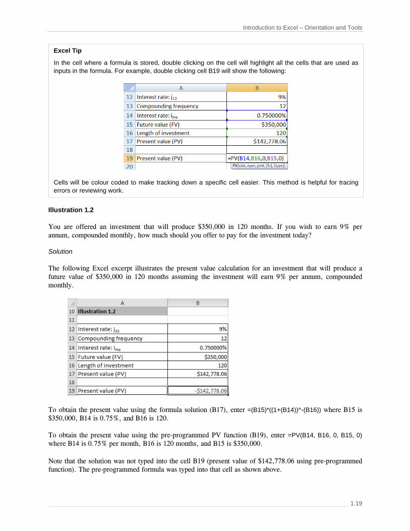
Illustration 1.2 You are offered an investment that will produce $350,000 in 120 months. If you wish to earn 9% per annum, compounded monthly, how much should you offer to pay for the investment today? Solution The following Excel excerpt illustrates the present value calculation for an investment that will produce a future value of $350,000 in 120 months assuming the investment will earn 9% per annum, compounded monthly.

To obtain the present value using the formula solution (B17), enter =(B15)*((1+(B14))^-(B16)) where B15 is $350,000, B14 is 0.75%, and B16 is 120. To obtain the present value using the pre-programmed PV function (B19), enter =PV(B14, B16, 0, B15, 0) where B14 is 0.75% per month, B16 is 120 months, and B15 is $350,000. Note that the solution was not typed into the cell B19 (present value of $142,778.06 using pre-programmed function). The pre-programmed formula was typed into that cell as shown above.

Excel Tip

In the cell where a formula is stored, double clicking on the cell will highlight all the cells that are used as inputs in the formula. For example, double clicking cell B19 will show the following:

Cells will be colour coded to make tracking down a specific cell easier. This method is helpful for tracing errors or reviewing work.

1.19

Lesson 1

Note that the compounding frequency of the interest rate must match the length of the loan or investment (NPER). In this example, the compounding frequency of the interest rate is monthly and the length of the investment is also in months. If the compounding frequency of the interest rate does not match the length of the loan, then an interest rate conversion is required … more on this topic in this next section. In addition, The TYPE of loan is a value representing the timing of the payment. If payments occur at the beginning of a period, the type is 1 and if at the end, the type is 0. Since there is no payment in this calculation, the type is 0 or can be omitted as 0 is the default option. Notice also that the result shows as a negative when we use the pre-programmed PV function. Since this illustration is examined from the investor's perspective, we enter the future value as a positive (cash inflow) and the present value produces a negative (cash outflow-amount invested). Note that if this illustration was examined from the borrower's perspective, we would enter the future value (amount to repay) as a negative (cash outflow) and the present value is a positive (cash inflow). There is no difference mathematically! You just have to recognize the timing of the cash flows from either the borrower or investor's perspective.

Positive and Negative Cash Flows: A Matter of Perspective

Financial calculators and spreadsheets, such as Excel, have the financial formulas programmed in, so that users need only specify the amounts and the computer does the math. However, a problem with any calculator/spreadsheet is in specifying positive and negative cash flows. For example, in a typical mortgage loan, the borrower receives loan funds at the beginning of the loan term (cash in, so a positive amount) and makes periodic payments during the loan term and an outstanding balance payment at the end of the loan term (cash out, so negative amounts). Excel requires opposite signs be used, so PV will be shown as positive, while PMT and FV will be shown as negatives. From the lender's perspective, this could be reversed with PV negative and PMT and FV positive; however, this difference has no mathematical impact. The need to specify negative cash flows or not will vary with every calculator and spreadsheet, depending on how it was programmed. You must be careful to ensure you are using your financial tool correctly, because one incorrect + or – and you will get incorrect answers.

"What If" Analysis

Similar to the calculator, in order to change an element, in this case, the future value, we only have to change the cell (B15) with a future value of $350,000 to $300,000; Excel will automatically recalculate the present value to $122,381.19.

Tips and Tricks: Excel Formulas

• Formulas OR Functions MUST BEGIN with an equal sign (=). • Don't type in the data itself into a function; instead, reference a cell where the data is specified, so that

you can easily change it later if you wish.

1.20


Future Value You can solve for the future value of interest accrual loans in Excel by either using the math formula or the pre-programmed financial function. Recall that the formula for the future value of interest accrual loans and investments is as follows:

FV = PV (1 + jm/m)n

where

jm = Nominal (annual rate of interest-j-) with a stated compounding frequency (m) PV = Present value FV = Future value after N periods n = Number of compounding or payment periods in the financial problem

The pre-programmed function in Excel calculates the future value for a loan or investment given the periodic rate, the number of periods, and the present value. The pre-programmed function for future value is =FV(RATE, NPER, PMT, PV, TYPE) where:

• RATE represents the periodic interest rate for the loan or investment • NPER represents the total number of payments • PMT represents the payment made or received each period (zero in this case) • PV represents the present value • TYPE represents when the payments are due (0 at the end of the period or omitted, 1 at the

beginning of the period)

Exercise 1.1 You are offered four investment opportunities that will produce the following amounts at the end of the term. The table below provides a summary of the investments. For each investment, calculate the amount to invest today in order to accumulate the desired future value.

Summary of Terms

Investment Term

(Years) Nominal Rate Amount Received at the End of Term

1 1 year j12 = 2% $2,000

2 5 years j2 = 7% $25,000

3 1.5 years j1 = 4% $3,500

4 8 years j4 = 10% $100,000 Abbreviated Solution 1. PV = $1,960.43 2. PV = $17,722.97 3. PV = $3,300.03 4. PV = $45,377.06

1.21

Lesson 1

Illustration 1.3 A commercial enterprise has arranged for an interest accrual loan whereby the $10,000 amount borrowed is to be repaid in full at the end of one year. The borrower has agreed, in addition, to pay interest at the rate of 8% per annum, compounded annually on borrowed funds and this interest is to be calculated and paid at the end of the loan's three-year term. Calculate the total amount owing at the end of the term of the loan. Solution The following Excel excerpt illustrates the future value calculation of an interest accrual loan of $10,000 at a rate of 8% per year, compounded annually for a 3-year term.

To obtain the future value using the formula (B27), enter =(B24)*((1+B23)^B25) where B24 is $10,000, B23 is 8%, and B25 is 3. To obtain the future value using the pre-programmed FV function (B29), enter =FV(B23, B25, 0, B24, 0) where B23 is 8%, B25 is 3 years, and B24 is $10,000. Again, notice that the compounding frequency of the interest rate must match the length of the loan or investment (NPER). In this example, if the compounding frequency was monthly and the length of the loan is three years, NPER must be entered as 36 (12 × 3). Notice also that the result shows as a negative when we use the pre-programmed FV function. Since this illustration is examined from the borrower's perspective, we enter the loan amount as a positive (cash inflow) and the future value is a negative (cash outflow-repayment of debt).

Outstanding Balance (OSB) Calculations in Excel

Note that we also use the pre-programmed FV function to determine OSB calculations of mortgage loans; this will involve a payment that represents the regular mortgage payment paid during the term of a mortgage loan. This topic is discussed in detail in a future section of this lesson.

1.22


Equivalent Interest Rates Two interest rates are equivalent if, for the same amount borrowed, over the same period of time, the same amount is owed at the end of the period. The nominal interest rate is an interest rate quoted as a rate per annum. The nominal rate is represented mathematically as "jm " where:

jm = nominal interest rate compounded "m" times per year m = number of compounding periods per annum i = interest rate per compounding period

The periodic interest rate represents the interest rate per compounding period. The nominal rate of interest compounded "m" times per year (jm) is equal to the periodic interest rate per compounding period (i) times the number of compounding periods per year (m). jm = i × m

Exercise 1.2 The table below provides a summary of four investment opportunities. For each investment, calculate the amount that will be received at the end of the term based on the amount invested, investment period, and interest rate earned.

Summary of Terms

Investment Amount to Invest

(Today) Terms (Years) Nominal Rate

1 $75,000 2 years j12 = 6%

2 $20,000 4 years j2 = 4%

3 $325,000 5 years j1 = 9.5%

4 $15,000 1.5 years j4 = 2% Abbreviated Solution 1. FV = $84,536.98 2. FV = $23,433.19 3. FV = $511,627.59 4. FV = $15,455.66

Rounding Rules Alert!

When calculating monetary amounts, numbers will have to be rounded off, since it is impossible to pay or receive an amount less than one cent. When rounding monetary amounts (e.g., PV, FV, or PMT), normal rounding rules are applied. This is the common mathematical rule which states:

• If the third decimal is 5 or greater, the number is rounded up: e.g. 8,955.436 would be rounded UP to $8,955.44 (because the third decimal is a 6).

• If the third decimal is less than 5, the number is rounded down: e.g. 8,955.433 would be rounded DOWN to $8,955.43 (because the third decimal is a 3).

Assume all monetary values are rounded to the nearest cent, unless instructed otherwise.

1.23

Lesson 1

And rearranging the formula, the periodic rate is equal to the nominal rate (j) divided by the compounding frequency (m) i = j ÷ m The effective annual interest rate (j1) is a nominal interest rate with yearly compounding. The effective rate is used to standardize interest rates to allow borrowers and lenders to compare different rates on a common basis.

Some problems may require "converting" between different interest compounding frequencies. For example, mortgage interest rates are nearly always stated as annual rates with semi-annual compounding (j2); however, most Canadian mortgage payment amounts are calculated on the basis of monthly payments. To be fully accurate in calculations, you need to account for the difference in the compounding for the stated rate and the rate needed for calculating payments.

Why Does Compounding Matter?

A part of "financial fluency" is being able to move between nominal, periodic, and effective rates effortlessly.

Consider a loan of $100,000 calling for monthly payments over 25 years at an interest rate of j2=12%. The monthly payments are $1,031.90. However, if the interest rate is incorrectly used as j12=12%, the monthly payments are $1,053.22. The $21.32 per month difference is not massive, but certainly a borrower would not want to pay any more extra interest than he or she has to, just as an investor would not want to give up any extra return to which the investor is entitled.

You may find that many practitioners simply ignore this impact of compounding differences and try to assume away the impact of compounding differences; e.g., assume that a j2=12% mortgage rate is simply a j12 and divide it by 12 to obtain the 1% monthly periodic rate. When working with a 30-year forecasted pro forma, with substantial future assumptions, this slight variation may not be significantly important. However, there is no question that it is mathematically sloppy (and inaccurate). If a more accurate number is available without substantial work, in our opinion it is a more sophisticated analysis, and a better showcase of your professionalism, to work with the most accurate numbers possible (rather than assume away the hard stuff…as the adage says “if it was that easy, what would they need you for!”

Equivalent Interest Rates

Two interest rates are equivalent if, for the same amount borrowed, over the same period of time, the same amount is owed at the end of the period.

You can solve for equivalent interest rates in Excel by programming in the mathematical formula:

Periodic Rate =((1+(Nominal Rate/Stated Frequency))^(Stated Frequency /Desired Frequency))-1

Or, you may use the pre-programmed functions, NOMINAL and EFFECT.

1.24


Illustration 1.4 Consider the following Excel excerpt where we change from a given rate of 6% per annum, compounded monthly (j12) to an equivalent nominal rate, compounded semi-annually (j2). Solution

To obtain the solution for the periodic rate (isa) using the mathematical formula, enter =((1+(B33/B34))^(B34/B35))-1 where B33 is 6%, B33 is 12, and B35 is 2. Note that the formula generates a semi-annual periodic rate of 3.037751%. To obtain the j2 equivalent of 6.075502%, we must multiply the semi-annual rate (B37) by the desired compounding frequency (B35) of 2. This mathematical formula solution can be used to solve any interest rate conversion problem. However, the syntax for this formula is difficult and prone to errors. A much simpler solution in Excel uses its pre-programmed functions, NOMINAL and EFFECT:

=NOMINAL(effective rate per year, N compounding periods per year) =EFFECT(nominal rate per year, N compounding periods per year)

These operate in much the same way as the NOM% and EFF% keys on the HP10BII/II+ calculator. Revising Illustration 1.4, we now use the Excel functions to find the periodic rate (isa) and the equivalent annual rate with semi-annual compounding (j2):

To obtain the equivalent j1 rate (B40), enter =EFFECT(B33,B34) where B33 is 6% and B34 is 12. The effective annual rate (j1) is 6.167781%. To obtain the j2 rate (B41), enter =NOMINAL(B40,B35) where B40 is 6.167781% and B35 is 2. The annual rate with semi-annual compounding (j2) is 6.075502%. To obtain the equivalent semi-annual rate (B42), enter =B41/B35 where B41 is 6.075502% and B35 is 2. The equivalent semi-annual rate (isa) is 3.037751%.

1.25

Lesson 1

Illustration 1.5 Consider an example where the interest rate of 9.6% is compounded semi-annually, that is, the interest rate given is semi-annual, while the payment period is monthly. Calculate the equivalent monthly interest rate (imo). Solution In order to find the equivalent monthly periodic rate, we have to first convert the interest rate to its effective (annual) rate, then convert it to its nominal interest rate with monthly compounding and finally divide by 12 to determine the monthly periodic rate. That is, we have to convert the j2 rate to the j12 rate, and then divide by 12 to find the periodic rate (imo). Using Excel to find the periodic rate, the solution is as follows:

To obtain the equivalent j1 rate (B48), enter =EFFECT(B46, B47) where B46 is 9.6% and B47 is 2. To obtain the equivalent j12 rate (B50), enter =NOMINAL(B48, B49) where B48 is 9.8034% and B49 is 12. To obtain the monthly interest rate (B51), enter =B50/B49 where B50 is 9.413447% and B49 is 12. Illustration 1.6 Consider another example where we want to change the interest rate from 4% per annum, compounded semi-annually (j2) to an equivalent monthly interest rate (imo). Solution The Excel excerpt is as follows:

To obtain the j1 equivalent rate of 4.04% (B57), enter =EFFECT(B55, B56) where B55 is 4% and B56 is 2. To obtain the j12 nominal rate (B59), enter =NOMINAL(B57, B58) where B57 is 4.04% and B58 is 12. To obtain the monthly interest rate (B60), enter =B59/B58 where B59 is 3.967068% and B58 is 12.

1.26


Exercise 1.3 The following table is comprised of three columns:

1. The first column specifies a nominal rate of interest with a given compounding frequency. 2. The second column provides the desired compounding frequency. 3. The third column presents an equivalent nominal interest rate with the desired frequency of

compounding.

Readers should ensure that they can use the nominal rates of interest and desired frequencies of compounding shown in the first two columns to calculate the equivalent nominal interest rate shown in the third column.

Nominal Interest Rate Desired number of

compounding periods per annum

Equivalent nominal interest rate with desired compounding

frequency

j12 = 4.50% j4 = 3.50% j4 = 7% j12 = 8.6% j2 = 6% j1 = 3%

1 12 2 365 12 2

j1 = 4.593983% j12 = 3.489841% j2 = 7.06125% j365 = 8.570336% j12 = 5.926346% j2 = 2.977831%

Exercise 1.4 The following table is comprised of three columns:

1. The first column specifies a periodic rate of interest with a given compounding frequency. 2. The second column provides the desired compounding frequency. 3. The third column presents an equivalent periodic interest rate with the desired frequency of

compounding.

Readers should ensure that they can use the periodic rates of interest and desired frequencies of compounding shown in the first two columns to calculate the equivalent periodic interest rate shown in the third column.

Periodic Interest Rate Desired number of

compounding periods per annum

Equivalent periodic interest rate with desired compounding

frequency

isa = 0.35% iq = 4.5% isa = 3.25% ia = 6.75% id = 0.0012% iw = 0.046%

52 12 4 365 2 1

iw = 0.013439% imo = 1.478046% iq = 1.612007% id= 0.017897% isa= 0.219239% ia= 2.420274%

1.27

Lesson 1

Payment We can easily add the payment element to the previous present value and future value calculations. In this section, we expand our discussion to incorporate a value for the payment. Using the pre-programmed PMT function, if we are determining mortgage loan payments, we enter the periodic rate, length of loan (NPER), present value, future value (0), and type (0). Note that we must match the payment frequency with the interest rate and the length of the loan. As a result, it may be necessary to calculate an equivalent interest rate using the EFFECT and NOMINAL functions. As we discussed previously, since we have cash flows going in and out, either the payment or the present value will be entered as a negative. Since mortgage calculations are typically examined from the borrower's perspective, we enter the loan amount as a positive and the payment will result in a negative. The PMT function in Excel calculates the monthly payment for a loan given the periodic interest rate, the number of periods to pay off the loan, and the amount of the loan. The pre-programmed function for PMT is =PMT(RATE, NPER, PV, FV, TYPE) where:

• RATE represents the periodic interest rate for the loan or investment • NPER represents the total number of payments • PV represents the principal or present value (negative value if you owe the money) • FV represents the future value • TYPE represents when the payments are due (0 at the end of the period or omitted, 1 at the

beginning of the period) NOTE: If you are not provided a FV or Type (as in the illustration below), you can omit them from your function. Illustration 1.7 A car loan for $12,000 is to be repaid by equal monthly payments over a 5-year period. The interest rate is 9.6% per annum, compounded monthly. Calculate the size of the required monthly payments. Solution Since the compounding frequency of the interest rate matches the payment frequency, the monthly payment can be calculated directly without determining an equivalent monthly payment.

To obtain the payment (B69), we enter =PMT(B66, B68*B65, B67, 0, 0) where B66 is 0.8%, B68 is 5 years, B65 is 12 months, and B67 is $12,000.

1.28


Since most of these mortgage loan illustrations are from the borrower's perspective, we enter the loan amount as a positive and the payment will result in a negative. The calculated monthly payments are $252.609168. Since borrowers cannot make payments which involve fractions of cents, the payments must be rounded to the nearest cent. It is standard practice, on a series of level payments, to round the payment amount to the nearest cent. Regular rounding rules will apply unless the facts indicate otherwise. Therefore, the payments on this loan would be $252.61. In this situation, this rounding shortens the actual amortization period of the loan slightly, which results in a reduced number of payments required and/or more typically a final payment on the loan which is smaller than the other payments.

To obtain the rounded payment (B70), enter =ROUND(B69, 2) where B69 is the unrounded payment of $252.609168 and 2 represents rounding to two decimal places.

This illustration may be slightly simplistic, since interest rates for mortgage loans in Canada are not typically quoted using monthly compounding, but as annual rates with semi-annual compounding (j2). Since borrowers prefer to make their payments monthly, interest rate conversions are often required when calculating the periodic payments of principal and interest to be made on a loan. If payments occur monthly, principal reductions occur monthly, and interest calculations must be made on a monthly basis. The nominal rate with semi-annual compounding must be converted to its equivalent rate with monthly compounding so that the amount of interest charged each month can be calculated. Illustration 1.8 calculates the equivalent nominal interest rates for a constant payment mortgage using the same method as outlined in previous illustrations.

Loan payments can be rounded up to any amount specified in a loan contract, for example to the next higher dollar, ten dollars, or even hundred dollars. Unless stated otherwise, round repeated payments to the nearest cent.

Rounding Payments in Excel

If payments are rounded to the nearest cent, you can use the pre-programmed ROUND function by indicating the values to be rounded and the number of digits to round. For dollar and cents rounding, choose 2 as the number of digits.

If payments are rounded up, you can use the pre-programmed ROUNDUP function by indicating the value to be rounded and the number of digits to round. To round up to the next higher dollar, enter 0 as the number of digits; to round up to the next higher ten dollars, choose -1 as the number of digits; and to round up to the next higher one hundred dollars, enter -2 as the number of digits.

With repeated payments that are rounded up, you can use the pre-programmed ROUNDUP function by indicating the value to be rounded and the number of digits to round. For dollars and cents rounding, choose 2 as the number of digits. To round up to the next higher dollar, enter 0 as the number of digits; to round up to the next higher ten dollars, choose -1 as the number of digits; and to round up to the next higher one hundred dollars, enter -2 as the number of digits.

1.29

Lesson 1

Illustration 1.8 A constant payment mortgage of $175,000 is to be repaid by monthly payments over a 25-year amortization period. The interest rate is 4% per annum, compounded semi-annually (j2 = 4%). What is the size of the required monthly payment to fully repay the loan? Solution Since the interest rate's compounding frequency does not match the payment frequency, we must first find an equivalent monthly interest rate and then we can calculate the monthly payment.

To obtain the payment (B82), enter =PMT(B79, B81*B77, B80, 0, 0) where B79 is 0.330589%, B81 is 25 years, B77 is 12, and B80 is $175,000. To obtain the rounded payment (B83), enter =ROUND(B82, 2) where B82 is the unrounded payment of $920.5354.

Exercise 1.5 A prospective borrower has contacted five lenders and has collected the information summarized below. Calculate, for each loan alternative, the required payment and round the payment to the nearest cent.

Loan Loan Amount Nominal Rate Amortization

Period Frequency of

Payment

1 $75,000 j2 = 4% 20 years monthly 2 $100,000 j1 = 7% 25 years quarterly 3 $51,125 j4 = 5% 240 months monthly 4 $60,000 j2 = 6.25% 25 years monthly 5 $260,000 j2 = 3.25% 25 years biweekly

Abbreviated Solution

1. N = 240 j12 = 3.967068% PV = $ 75,000 PMT = $453.18 2. N = 100 j4 = 6.823410% PV = $100,000 PMT = $2,091.14 3. N = 240 j12 = 4.979310% PV = $ 51,125 PMT = $336.82 4. N = 300 j12 = 6.170140% PV = $ 60,000 PMT = $392.85 5. N = 650 j26 = 3.225876% PV = $ 260,000 PMT = $582.98

1.30


Rate The pre-programmed RATE function in Excel calculates the interest rate per period on a loan or investment given the periodic rate, the number of periods, and the present value. The pre-programmed function for interest rates =RATE(NPER, PMT, PV, FV, and TYPE) where:

• NPER represents the total number of payments in the loan or investment • PMT represents the payment made or received each period • PV represents the present value • FV represents the future value • TYPE represents when the payments are due (0 at the end of the period or omitted, 1 at the

beginning of the period) Notice that the pre-programmed function works to solve for interest rates involving loans and investments with and without payments (interest accrual loans). Illustration 1.9 provides an example of a rate calculation on an interest accrual loan and Illustration 1.10 provides an example of a rate calculation involving regular payments. Illustration 1.9 An individual deposits $15,000 in an account bearing interest that will grow to $20,000 in five years. The investor intends to let the interest accrue on this deposit and then invest the total amount in real estate. If the funds are deposited for a five-year period and accumulate to the desired future value, what interest rate must the investor earn in order to accumulate this amount, expressed as an effective annual rate (j1)? Solution

To obtain the RATE (B90), we enter =RATE(B89, 0, -B87, B88, 0) where B89 is 5 years, B87 is $15,000, and B88 is $20,000. In this example, there is no payment and the calculated periodic rate (annual) is the desired rate (annual); therefore, no additional interest rate calculations are required. We must enter the PV or the FV amounts as a negative in order to obtain a solution. As previously discussed, from an investor's perspective, we enter the present value as a negative and the future value as a positive.

1.31

Lesson 1

Illustration 1.10 A mortgage calls for monthly payments of $8,469.44 over 25 years. If the original loan advanced was $1,400,000, calculate the annual rate of interest with semi-annual compounding (j2). Solution Since the loan calls for monthly payments, one must first determine the nominal rate of interest with monthly compounding (j12), and then convert this result to an equivalent nominal rate with semi-annual compounding (j2).

To obtain the periodic monthly interest rate (B100), we enter =RATE(B98*B96, -B95, B97, 0, 0) where B98 is 25 years, B96 is 12 months, B95 is $8,469.44, and B97 is $1,400,000. Note also that either the present value or payment must be entered as a negative in order to obtain a solution. Since this loan is created from the borrower's perspective, we enter the payment as a negative and the loan amount as a positive. Note that the interest rate calculated is a periodic rate (in this case monthly). Multiply by the original compounding frequency (12) and then use the EFFECT and NOMINAL functions to obtain the equivalent j2 rate. To obtain the j1 rate (B102), enter =EFFECT(B101, B96) where B101 is 5.346594% and B96 is 12. To obtain the equivalent j2 rate (B103), enter =NOMINAL(B102, B99) where B102 is 5.479579% and B99 is 2. The interest rate on this $1,400,000 loan with monthly payments of $8,469.44 over 25 years is j2 = 5.406503%.

1.32


Loan or Investment Period The pre-programmed NPER function in Excel calculates the number of periods for a loan or investment given the periodic rate, the payment, present value, and future value. The pre-programmed function for the length of the loan or investment =NPER(RATE, PMT, PV, FV, and TYPE) where:

• RATE represents the periodic interest rate for the loan or investment • PMT represents the payment made or received each period • PV represents the present value • FV represents the future value • TYPE represents when the payments are due (0 at the end of the period or omitted, 1 at the

beginning of the period) Notice that the pre-programmed function works to solve for number of periods involving loans and investments with and without payments (interest accrual loans). Illustration 1.11 provides an example of a NPER calculation on an interest accrual loan and Illustration 1.12 provides an example of a NPER calculation involving regular payments.

Exercise 1.6 A private investor is considering three alternative mortgage investments, each of which involves a $60,000 loan amount:

1. Under the first alternative, the investor will receive 60 monthly payments of $1,104.93 2. Under the second alternative, the investor will receive 66 monthly payments of $1,025.05 3. Under the third alternative, the investor will receive 54 monthly payments of $1,207.48

Assist the investor in choosing among these alternatives by calculating the yield, as a nominal rate with semi-annual compounding, in each case.


1. j12 = 3.997735%, j2 = 4.031179% 2. j12 = 4.395223%, j2 = 4.435666% 3. j12 = 3.684914%, j2 = 3.713319%

The investor should choose the second alternative since it provides the highest return (rate of interest).

The amortization period is the period of time that it takes to fully pay off a loan, given the required periodic payments. Most lenders will state the amortization period they require. The stated amortization period is then used to calculate the size of the required payments, i.e., to fully pay off the loan's principal plus all interest owing over this specified time period. The maximum amortization period for insured mortgages is 25 years. For uninsured mortgages, the maximum is typically 30-35 years, depending on the lender.

1.33

Lesson 1

Illustration 1.11 An individual has placed $5,000 in a long-term saving accounts that will grow to $6,500 at an effective annual rate of 3.5% (j1=3.5%). Calculate how many years the funds must be invested in order to accumulate at least the desired amount. Solution

To obtain the investment period (B111), enter =NPER(B107/B108, 0, -B109, B110, 0) where B107 is 3.5%, B108 is 1, B109 is $5,000, and B110 is $6,500. Note that we must enter either the PV or the FV amounts as a negative in order to obtain a solution. As previously discussed, from an investor's perspective, we enter the present value as a negative and the future value as a positive. In order to accumulate at least the desired amount, the funds must be invested for 8 years. Illustration 1.12 To facilitate the sale of his property, a seller has agreed to provide partial financing to a buyer. Under this mortgage, the seller will loan the buyer $50,000, at a rate of 8% per annum, compounded semi-annually (j2 = 8%). The required payments are $684.51 per month. What is the amortization period for this loan?

Solution

Since the contract rate is compounded semi-annually and the payments are made monthly, the stated interest rate must first be converted and expressed as an equivalent nominal rate with monthly compounding; then we can calculate the amortization period of the loan.

To obtain the amortization (B122), enter =NPER(B119/B118, -B121, B120, 0, 0) where B119 is 7.869836%, B118 is 12, B121 is $684.51, and B120 is $50,000.

1.34


Either the PV or FV must be entered as a negative in order to find a solution. The amortization will generate a solution in periodic (monthly) terms; in order to calculate the amortization in years (B123), we must divide the monthly amortization by 12 to obtain the amortization of 8.313058 years (=B122/B118 where B122 is 99.756695 months and B118 is 12). The amortization period is 99.756695 months (approximately 100 months or 8.3 years).

Outstanding Balance (OSB) The loan's outstanding balance (OSB), the amount of principal owing at a specific point in time, may need to be calculated for several reasons. The pre-programmed future value function in Excel calculates the outstanding balance on a loan given periodic rate, number of periods, payment, and present value. The pre-programmed function for an outstanding balance (future value) is =FV(RATE, NPER, PMT, PV, TYPE) where:

• RATE represents the periodic interest rate for the loan or investment • NPER represents the total number of payments • PMT represents the payment made or received each period • PV represents the present value • TYPE represents when the payments are due (0 at the end of the period or omitted, 1 at the


Exercise 1.7 For each set of loan terms below, calculate the appropriate amortization period.

Loan Loan Amount Nominal Rate Payment

1 $100,000 j12 = 5% $659.96 per month 2 $100,000 j2 = 6% $839.89 per month 3 $50,000 j1 = 10% $6,000.00 per year 4 $62,500 j2 = 11.5% $623.40 per month 5 $451,000 j2 = 5.5% $1,100 per month


1. j12= 5% N = 239.997341 months 2. j12= 5.926346% N = 179.997514 months 3. j1= 10% N = 18.799246 years 4. j12= 11.233783% N = 299.374382 months 5. j12= 5.438018% N = No Solution

For loan 5, try increasing the payments to find the point at which they are large enough to amortize the loan.

Error Messages

If the payment is not large enough to repay the loan amount, an error message, #NUM, appears in the cell. This error also occurs if the Excel user forgets to enter the correct sign for the PMT or PV.

Outstanding balance (OSB)

The amount of principal owing on a loan at a specific point in time.

1.35

Lesson 1

Illustration 1.13 A $60,000 mortgage loan, written at j12 = 6%, has a 3-year term and monthly payments based upon a 20-year amortization period. Payments are rounded to the nearest cent. What is the outstanding balance of the mortgage at the end of its term? i.e., what is the outstanding balance just after the 36th payment (OSB36) has been made? Solution In order to calculate the outstanding balance for a mortgage, we first calculate the regular payment, round the payment, and determine the outstanding balance based on the rounded payment.

To obtain the payment (B133), enter =PMT(B127/B129, B131*B129, B130, 0, 0) where B127 is 6%, B129 is 12, B131 is 20, and B130 is $60,000. To obtain the rounded payment (B134), enter =ROUND(B133, 2) where B133 is the unrounded payment of $429.8586. To obtain the outstanding owing at the end of the three-year term (B135), enter =FV(B127/B129, B132*B129, B134, B130, 0) where B127 is 6%, B129 is 12, B132 is 3 years, B134 is $429.86, and B130 is $60,000. Since this loan is partially amortized, the borrower will make 36 monthly payments of $429.86 and pay the remaining balance of $54,891.81 at the end of the 36th month.

Exercise 1.8 For each of the first four loans in Exercise 1.7, assume each loan has a two-year term and calculate the outstanding balance owing at the end of the term.


1. OSB = $93,872.43 2. OSB = $91,206.14 3. OSB = $47,900.00 4. OSB = $61,474.51

1.36


Principal and Interest Components of Payments In addition to the outstanding balance, it may be necessary to calculate the principal and interest components of payments on constant payment mortgages. These calculations are important because interest on payments can sometimes be deducted as an expense for income tax purposes. As well, borrowers like to know how much principal they have paid off in a single payment or over a series of payments. The pre-programmed functions, IPMT and PPMT, can be used to calculate the interest and principal portions of individual payments. The pre-programmed function for IPMT is =IPMT(RATE, PER, NPER, PV, FV, TYPE) and the pre-programmed function for PPMT is =PPMT(RATE, PER, NPER, PV, FV, TYPE) where:

• RATE represents the periodic interest rate for the loan or investment • PER represents the period that you want to find the interest or principal (between 1 and NPER) • NPER represents the total number of payments • PV represents the present value • FV represents the future value • TYPE represents when the payments are due (0 at the end of the period or omitted, 1 at the

beginning of the period) The pre-programmed functions, CUMIPMT and CUMPRINC, can be used to calculate the interest and principal paid or received over a period of time. The pre-programmed function for CUMIPMT is =CUMIPMT(RATE, NPER, PV, START PERIOD, END PERIOD, TYPE) and the pre-programmed function for CUMPRINC is =CUMPRINC(RATE, NPER, PV, START PERIOD, END PERIOD, TYPE) where:

• RATE represents the periodic interest rate for the loan or investment • NPER represents the total number of payments • PV represents the present value • START PERIOD represents the first period in the calculation • END PERIOD represents the last period in the calculation • TYPE represents when the payments are due (0 at the end of the period or omitted, 1 at the


Illustration 1.14 Three years ago, Tom and Nancy bought a house with a mortgage loan of $175,000, written at j2 = 9.5%, with a 25-year amortization, a 3-year term, and monthly payments rounded up to the next higher dollar. Tom and Nancy are about to make their 36th monthly payment, the last one in the loan=s term, and want to know the following information:

a. How much interest will they be paying with their 36th payment? b. How much principal will they be paying off with their 36th payment? c. What will the outstanding balance be immediately following the 36th payment, i.e., the amount they

will have to refinance after the 36th payment? d. How much interest did they pay over the entire 3-year term? e. How much principal did they pay off during the 3-year term? f. What is the total amount of interest paid during the second year of the loan?

Payment Rounding

Note that these functions calculate the payment, but do not account for rounding – as a result, answers will differ slightly. If you want maximum accuracy in determining the principal and interest components, for NPER you need to enter the revised amortization period found by rounding off the payment and then re-computing N.

1.37

Lesson 1

Solution

To obtain the interest portion of the 36th payment (B151), enter =IPMT(B143/B142, B146*B142, B149, B144, 0, 0) where B143 is j12 of 9.31726%, B142 is 12, B146 is 3 years, B149 is the revised amortization of 299.8413017 months, and B144 is $175,000. To obtain the principal portion of the 36th payment (B152), enter =PPMT(B143/B142, B146*B142, B149, B144, 0, 0) where B143 is j12 of 9.31726%, B142 is 12, B146 is 3 years, B149 is the revised amortization of 299.8413017 months, and B144 is $175,000.

Alternative Solution To obtain the interest portion of the 36th payment (B155), enter =(D155*B143/B142) where D155 is OSB35, B143 is j12 of 9.31726%, and B142 is 12. To obtain the principal portion of the 36th payment (B156), enter =(B148–B155) where B148 is the rounded up payment of $1,507 and B155 is the interest portion of the 36th payment of $1,312.68.

To obtain the interest paid over the term (B160), enter =CUMIPMT(B143/B142, B149, B144, 1, B146*B142, 0) where B143 is j12 of 9.31726%, B142 is 12, B149 is the revised amortization of 299.8413017 months, B144 is $175,000, and B146 is 3 years.

1.38


To obtain the principal paid over the term (B161), enter =CUMPRINC(B143/B142, B149, B144, 1, B146*B142, 0) where B143 is j12 of 9.31726%, B142 is 12, B149 is the revised amortization of 299.8413017 months, B144 is $175,000, and B146 is 3 years. To obtain the interest paid during year 2 (B163), enter =CUMIPMT(B143/B142, B149, B144, 13, 24, 0) where B143 is j12 of 9.31726%, B142 is 12, B149 is the revised amortization of 299.8413017 months, and B144 is $175,000. Note that 13 represents the first payment in the second year and 24 represents the final payment in the second year.

Net Present Value (NPV) The pre-programmed NPV function in Excel calculates the net present value of an investment given the periodic interest rate and values for the future cash flows. The pre-programmed function for net present value =NPV(RATE,VALUE 1…VALUE N) where RATE represents the periodic interest rate for the loan or investment and VALUES represent the future cash flows (positive or negative) equally spaced in time and occurring at the end of each period. In financial calculations, the net present value is used by investors to compare investment alternatives. The calculated NPV is a dollar figure representing the present value of benefits less the present value of costs at the investor's required rate of return. If the rate of return is 20%, a positive NPV means the return on the investment is greater than 20%, given the cash flows indicated. If the NPV is negative, then the return on the investment is less than 20%. A quirk in how Excel calculates NPV: the values specified start at the beginning of the first period, e.g., if the investment period is in years, then it assumes the first cash flow is at the end of Year 1. This is not realistic for most investments, as the initial capital expenditure is immediate, at the start of Year 1 (sometimes called Year 0), with the first cash flow returned at the end of Year 1.

Exercise 1.9 For each set of loan terms below, calculate the monthly payment, the interest paid in the 3rd month, the principal paid in the 29th month, and the total interest paid during the first year of the loan.

Loan Loan Amount Nominal Rate Amortization

1 $100,000 j12 = 5% 20 years

2 $200,000 j2 = 6% 25 years

3 $90,000 j1 = 9% 20 years

4 $375,000 j2 = 4.5% 25 years Abbreviated Solution

Loan Payment Interest Principal Interest Yr 1 1 $100,000 $659.96 $414.63 $273.33 $4,932.16 2 $200,000 $1,279.61 $984.83 $335.06 $11,755.97 3 $90,000 $789.54 $646.62 $172.26 $7,715.26 4 $375,000 $2,075.52 $1,388.17 $756.93 $16,549.54

Tips and Tricks

Rather than filling in each individual value, you can place the cursor in the textbox beside Value 2 and then use the mouse to select all of the individual cash flows.

1.39

Lesson 1

Illustration 1.15 For example, assume you have an investment that costs you $100 today, and pays you $10 in one year, $14 in two years, and then $120 in three years. The discount rate is an effective annual rate of 10%. Calculate the present value of the cash flows and the net present value of this investment. Solution

If you use the NPV function in Excel, the pre-programmed function is as follows: =NPV(B173, B169:B171) where B173 is 10% and B169-B171 represent the cash flows for years 1-3. This calculation produces a NPV of $110.82; this determines the present value of the future cash flows (Years 1-3) at a yield of 10%. However, this result does not consider the cost of the investment (paid at time 0). To obtain the net present of this investment, we take the calculated present value of the cash flows and subtract the initial cost. In Excel, the general solution is as follows:

=NPV(RATE, CF1:CFN)+CF0

For Illustration 1.15, the net present value (B176) is =NPV(B173, B169:B171)+ B168 where B173 is 10%, B169-B171 are the cash flows for Years 1-3, and B168 is the initial investment of -$100. Note that since B168 is shown as a negative on the spreadsheet, we add that negative value to the present value of the cash flows to obtain the correct net present value. The NPV is now correctly calculated to be $10.82.

NPV Function in Excel

There is an anomaly in Excel's NPV function, compared to how NPV is normally calculated. Excel's NPV function is actually calculating the present value of future cash flows only. The present value net of initial cost must be calculated manually by subtracting these initial costs from Excel's calculated (so-called) NPV. It is worth noting that the IRR function in Excel already takes this initial cost issue into account and correctly calculates the internal rate of return (IRR), which is discussed in the next section.

1.40


Illustration 1.16 A local real estate investment group is considering the acquisition of a real estate investment. The forecasted annual net cash flows are as follows:

Year Net Cash Flow

0 –$45,000

1 12,000

2 12,800

3 13,600

4 14,400

5 15,000 The investment group would like to earn at least 5% per annum, compounded annually, on their investment. Calculate the present value and the net present value of this investment. Solution

To obtain the present value of the investment (B196), enter =NPV(B194, B188:B192) where B194 is 5% and B188-B192 are the cash flows from years 1-5. To obtain the NPV of this investment (B199), enter NPV(B194, B188:B192) + B198) where B194 is 5%, B188-B192 are the cash flows from years 1-5, and B198 is the initial investment of $45,000 (negative).

Tips and Tricks

Rather than retyping a formula into another cell, such as the NPV formula in B199 in the above illustration, which is also typed in B196, you can enter the following in B199: =B196+B198. This will give you the same result – see Illustration 1.16 in the Excel file, "CPD 152 –- Lesson 1 Solutions" to see how this is entered.

1.41

Lesson 1

Internal Rate of Return Internal rate of return (IRR) is another important financial function in Excel. Where NPV calculates the present value dollar return given a discount rate, IRR will calculate the interest rate return on capital. The pre-programmed IRR function will have the following instructions:

Values Initial cost (negative) and subsequent periodic net cash flows

Guess 0.2 (rough estimate of IRR, to give software a starting point for its calculation)

Tip: rather than filling in each individual value, you can place the cursor in the Values blank space and then use the mouse to highlight all of the series of individual cash flows. Using Illustration 1.15, The IRR (expressed as percentage) is calculated as follows:

To obtain the IRR for this investment (B183), enter =IRR(B179:B182,10) where B179-B182 represent the cash flows beginning with the initial investment (as a negative) followed by all future cash flows and 10 represents a percentage guess for the IRR. Illustration 1.17 A local real estate investment group is considering the acquisition of a real estate investment. The forecasted annual net cash flows are as follows:

Year Net Cash Flow

0 –$275,000

1 $14,000

2 $20,000

3 $25,000

4 $25,000

5 $360,000 The investment group would like to earn at least 8% per annum, compounded annually, on their investment. Calculate the internal rate of return for this investment.

1.42


Solution

To obtain the IRR for this investment (B213), enter =IRR(B204: B209, 8) where B204 represents the initial investment (negative), B205-B09 represent the future cash flows, and 8 represents a guess for the IRR. The IRR of this investment is approximately 11.2%, greater than the investor's desired yield of 8%.

Exercise 1.10 A local real estate investment group is considering the acquisition of a real estate investment. The forecasted annual net cash flows for four potential investments are as follows:

Year Investment 1

Net Cash Flow Investment 2



Net Cash Flow

0 -$275,000 -$275,000 -$275,000 -$275,000

1 $12,000 $15,000 $10,000 $18,000

2 $18,000 $15,000 $20,000 $18,000

3 $20,000 $18,000 $20,000 $18,000

4 $22,000 $18,000 $25,000 $24,000

5 $300,000 $320,000 $375,000 $350,000

For each of the investment opportunities, calculate the IRR and the NPV at a yield of 6% per annum, compounded annually. Which is the best investment opportunity on the basis of NPV and IRR?


Investment 1: IRR = 6.908%; NPV = $10,736.59 Investment 2: IRR = 7.742%; NPV = $20,994.34 Investment 3: IRR = 11.3436%; NPV = $69,050.43 Investment 4: IRR = 10.3113%; NPV = $53,664.82

On the basis of NPV and IRR only, the best investment is Investment 3; generating the largest NPV and IRR.

1.43

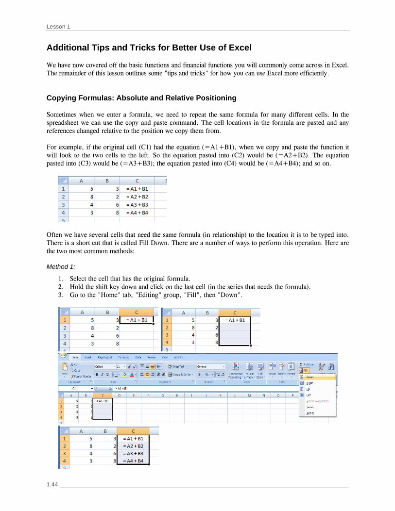
Lesson 1

Additional Tips and Tricks for Better Use of Excel We have now covered off the basic functions and financial functions you will commonly come across in Excel. The remainder of this lesson outlines some "tips and tricks" for how you can use Excel more efficiently. Copying Formulas: Absolute and Relative Positioning Sometimes when we enter a formula, we need to repeat the same formula for many different cells. In the spreadsheet we can use the copy and paste command. The cell locations in the formula are pasted and any references changed relative to the position we copy them from. For example, if the original cell (C1) had the equation (=A1+B1), when we copy and paste the function it will look to the two cells to the left. So the equation pasted into (C2) would be (=A2+B2). The equation pasted into (C3) would be (=A3+B3); the equation pasted into (C4) would be (=A4+B4); and so on.

Often we have several cells that need the same formula (in relationship) to the location it is to be typed into. There is a short cut that is called Fill Down. There are a number of ways to perform this operation. Here are the two most common methods: Method 1:

1. Select the cell that has the original formula. 2. Hold the shift key down and click on the last cell (in the series that needs the formula). 3. Go to the "Home" tab, "Editing" group, "Fill", then "Down".

1.44


Method 2:

1. Select the cell that has the original formula. 2. Hold your mouse on the dot on the right bottom corner of the cell. 3. Without releasing your mouse drag the cursor down to the last cell (in the series that needs the

formula). 4. Release the mouse.

Sometimes when you are copying a formula, it is necessary to keep a certain position that is not relative to the new cell location. For example, if you are producing an amortization table, you would want all the cells that calculate the payment to refer to a single set of data (i.e., the term or the interest rate) contained in one or more fixed cells. This is possible by inserting a $ before the column letter and/or a $ before the row number. This is called Absolute Referencing. Following our example, if we were to fill down with this formula we would have the exact same formula in all of the cells C1, C2, C3, and C4. The dollar signs lock the cell location to a fixed position. When it is copied and pasted it remains exactly the same (not relative).

We can also fill right. We must select the original cell (and the cells to the right) and select from the Edit menu–Fill and Right (Excel 2007: "Home" tab, "Editing" group, "Fill", then "Right").

1.45

Lesson 1

If we were to fill right from A1 to C1 we would get the formulas displayed in the table below. Notice that the second part of the equation is fixed or absolute reference, so always reference B3 which is 10.

Answers across Row 1 would be A1=16, B1=12, C1=15 (below).

Formatting Spreadsheets can be pretty dry, so we need some tools to dress them up a little. Adding colored text, borders, and highlighted cells can help organize information and make for a more visually appealing presentation. We can use most of the tricks in our word processor to do the formatting of text. We can use things like: bold face, italics, underline, different colors of both text and cell background, different alignments (left, right, centre), and changes in font size and font type, as well as setting the number of decimal places. We need to select the cell (or group of cells) that we wish to change the formatting and then use the "Home" tab; the "Font" group, "Alignment" group, and "Number" group all have various "quick formats" that you can use.

A scan across the ribbon shows in the "Font" group the font type and size, bold, italic, underline, borders, color fill, and text color; in the "Alignment" group vertical and horizontal alignment within cells, orientation, left and right indent, text wrapping and cell merging; and, in the "Number" group, style, currency, percentage, and comma formats, as well as increase or decrease the decimal.

1.46


If you want more options than those offered on the ribbon, click on the bottom-right corner of any of the three groups: "Font", "Alignment", or "Number". The following window will be displayed; there are several options beyond what is available on the ribbon.

As mentioned previously, we can change the format of numbers within cells. This means things like displaying the appropriate number of decimals, showing currency signs, percentage, even red numerals for negative dollars. It is best to keep numbers describing similar items as uniform as possible, and the count of decimal places reasonable…if all of your numbers are in dollars and cents, there is not much point in an interest rate being 15 decimal places. If we have the number 3.532626246724217, we would probably have to make the column wider and at the least bore most people. We need to set the number of decimal places to what is important. If this was a dollar figure that represented a calculated sales tax it should be formatted as $3.53. Below is a screen displaying what you would see if you select a cell (or group of cells) and then use the "Home" tab and click on the bottom-right corner of the "Number" group (or click on the Number tab shown on the Format Cells window previously). The first screen sample shows the General format (which is the default) and the second the Number format with choices for a thousands separator, red negative numbers, and number of decimal places.

1.47

Lesson 1

A question that everyone who has ever worked on a spreadsheet has asked at one time or another is, "Where did all my numbers go?" or a similar question, "Where did all of those ####### come from and why are they in my spreadsheet?" The problem is that the number trying to be displayed in a particular cell is too wide for the cell to display properly. To clear up the problem we just need to make the column wider. You can do this many ways. Here are three ways to change the column width:

1. Select the column (or columns) by clicking on their labels (letters), then on the "Home" tab, "Cells" group, then "Format". Click Column Width and type in a new number for the column width in the small window. The selected columns will have a new width. The example below changes the widths of Columns A, B, and C to 22 (from 8.43).

1.48


2. Move the mouse (arrow) to the right side of the column label (see the following figure) and click and drag the mouse to the right (to make wider) or left (to make smaller). Notice that the cursor changes to a vertical line with arrows pointing left and right. Let up on the mouse button when the column is wide enough.

3. You could also double click the mouse button between the column labels, as shown in the figure above. This will automatically resize your column so that it will be large enough to display the largest number or label in that column.

In many spreadsheets you can also change the vertical height of a row by moving the lower edge of the row title (number). If you have a spreadsheet designed and you forgot to include some important information, you can insert a column into an existing spreadsheet. What you must do is click on the column label (letter) and on the "Home" tab, "Cells" group, "Insert", then "Insert Sheet Columns". This will insert a column immediately left of the selected column. The following example will insert a new column between the current Columns B and C.

As you can see from this example, there was a blank column inserted into the spreadsheet… a new Column C. The old Column C is now Column D, the old Column D is now Column E, and the old Column E is now F. You might wonder if this will affect your referenced formulas. The referenced cells are changed to their new locations. For example: C4 =C3+B4 BECOMES C4 =D3+B4

1.49

Lesson 1

Likewise, we can also insert rows. With the row label (number) selected you must choose the "Insert Sheet Rows" from the Insert menu. Again, this will insert a row above the row you have selected. The following example will insert a new row between the current Rows 2 and 3.

The old Row 3 is now Row 4 and the old Row 4 is now Row 5. The formulas will be updated to their corresponding locations. C3 =C2+B3 BECOMES C4 =C2+B4

Multiple Worksheets Within Excel you can open and use multiple worksheets in one file. At the bottom of the Excel screen there are three tabs called "Sheet1", "Sheet2", and "Sheet3". You can click on a new tab to start working on a separate spreadsheet. You can also rename those tabs (Question 1, Question 2, etc.) by right clicking on the tab and selecting "Rename". Additionally, you can create further worksheets by clicking on the "Insert Worksheet" tab. When working on one spreadsheet you can link to a cell in another spreadsheet by clicking on the spreadsheet tab you want to go to, clicking the appropriate cell, and then returning to your original spreadsheet. NOTE: You should only link to cells within the same Excel file, otherwise, when you close the second file your functions will not work.

1.50


Hiding Columns and Rows Within Excel you can hide columns and rows if you want to simplify your spreadsheet. To hide a column, right click on the column header (B, for example) and select "Hide". To unhide your column, highlight the headers to the right and left of your hidden column (A and C, for example) and select "Unhide". The same applies for hiding and unhiding rows.

Freezing Rows and Columns In Excel, you can freeze panes to keep specific rows or columns visible when you scroll in the worksheet. For example, you might want to keep row and column headings visible when you scroll. In order to freeze rows or columns:

1. On the worksheet, do one of the following:

• To lock rows, select the row below the row or rows that you want to keep visible when you scroll.

• To lock columns, select the column to the right of the column or columns that you want to keep visible when you scroll.

• To lock both rows and columns, click the cell below and to the right of the rows and columns that you want to keep visible when you scroll. TIP: To cancel a selection of cells, click any cell on the worksheet

2. On the View tab, in the Window group, click the arrow below Freeze Panes.

3. Do one of the following:

• To lock one row only, click Freeze Top Row. • To lock one column only, click Freeze First Column. • To lock more than one row or column, or to lock both rows and columns at the same time, click

Freeze Panes. To unlock frozen columns or rows go to the View tab, in the Window group, and click "Unfreeze Panes".

1.51

Lesson 1

Summary This lesson has provided an orientation to the Microsoft Excel spreadsheet program. We examined the components of a spreadsheet, explained the types of data and calculated many of the basic mathematical and financial operations. The majority of the lesson was spent on the financial functions of Excel, with illustrations focusing on both financing and investment scenarios. We finished the lesson with a summary of some tips and tricks for using Excel to its maximum potential, both in terms of carrying out calculations and presenting them in a professional manner. In Lesson 2 we will build on this orientation by looking at the application of Excel in three practical real estate contexts: amortization schedules, discounted cash flow analysis, and reserve fund studies. All of these applications are built upon the tools introduced in Lesson 1.

1.52


Review and Discussion Questions 1. View the "Insert Function" menu in Excel (in Excel 2013, this is Formulas…Insert Function).

Investigate additional financial functions not covered in this lesson and test them out in Excel, using the examples provided in the lesson or your own examples.

Open and download the file found under Lesson 1 on the course website: "CPD 152 – Excel Practice Lesson 1". Here you will find all of the data pertaining to Questions 2 to 5. All of your work can be completed in this file. Furthermore, you will find a solution below each question. To maximize learning, solve the question on your own before consulting the solution.

2. a. Calculate the future value of the three interest accrual loans. Which loan produces the greatest

future value? b. Determine the payment and outstanding balance at the end of the term. (Hint: determine the

payment first). c. Determine the principal and interest components of the payment. d. Determine the IRR and NPV for the given investments. Which investment would you choose? 3. The real estate management firm you work for needs you to total all the rents from all of their

commercial properties over the past month. Provide a total for the rent of each property (Property totals), and a total of all rents from all properties (Portfolio Total).

4. You are analyzing recent sales transactions of single family homes in a small neighbourhood. Determine

the MEAN, MAXIMUM, and MINIMUM of the given sales data. 5. Write an IF formula so that if the number in the yellow highlighted cell is 200, then the cell containing

the IF formula will equal 1. If the number in the yellow highlighted cell is not 200, then the formula shows 0.

1.53

Documents

DISCLAIMER: © Copyright: 2014