direct displacement based design(DDBD)

ISSN: 0871-7869

Direct Displacement Based Design of a RC Frame – Case of Study

B. Massena; R. Bento; H. Degée

- Novembro de 2010 -

Relatório ICIST DTC nº 08/2010

Index

1.! Introduction ........................................................................................................................ 1!2.! Direct Displacement Based Design Method for Reinforced Concrete Frames .................. 1!

3.! Case of study- Reinforced Concrete Frame ...................................................................... 13!3.1. Direct Displacement Based Design for a peak ground Acceleration of 0.35g ................. 14!

3.2. Direct Displacement Based Design for a peak ground acceleration of 0.27g .................. 25!4.! Final remarks .................................................................................................................... 29!

5.! References ........................................................................................................................ 30!

1

1. Introduction

Over the last years, as the importance of displacements, rather than forces, has become better appreciated,

a growing interested appeared for methods based on displacements, in particular for what regards RC

structures. Several contributions were made towards the development of Displacement Based Design

(DBD) approaches, but it was only in the 1990’s that formal proposals were made to implement the

emerging ideas into formalized design procedures. One of these new design procedures is the Direct

Displacement Based Design, which was developed on the base of Priestley works [1, 2]. The central idea

of the Direct Displacement Based Design (DDBD) procedure is to design structures in order to achieve

displacements corresponding to a given seismic hazard level.

The objective of this study is to apply the Direct Displacement Based Design to a simple case of study, a

reinforced concrete frame building and to assess the applicability of the method and the needed of

develop an automatic design tool [3].

2. Direct Displacement Based Design Method for Reinforced Concrete Frames

The step by step DDBD procedure is listed in the following:

Step 1: Definition of the target displacement shape and amplitude of the MDOF structure on the base of

performance level considerations (material strain or drift limits) and then derive from there the design

displacement Δd of the substitute SDOF structure of the MDOF.

Fig.1 presents a simplified model of a multi-storey frame building, where is shown the required variables

in DDBD procedure.

Figure 1: Simplified model of a multi-storey building

where, δi is the normalised inelastic mode shape, mi are the masses at each significant storey i, me is the

equivalent mass of the SDOF, Hi is the height of each storey, Hn are the total height of the building, He is

the equivalent height and Δd is the equivalent SDOF design displacement.

2

- Displacement Shape

The normalised inelastic mode shape δi of the frame MDOF structure is defined in Ref. [2] and should be

obtained according to the number of stories, n, as:

n

ii HHnfor =≤ δ:4 (1)

!!"

#$$%

&−⋅!!

"

#$$%

&⋅=>

n

i

n

ii H

HHHnfor

41

34:4 δ (2)

The design storey displacements Δi are found using the shape vector δi, defined from Eq. (1) or Eq. (2),

scaled with respect to the critical storey displacement Δc and to the corresponding mode shape at the

critical storey level δc. According to Ref. [2], the design storey displacements for frame buildings will

normally be governed by drift limits in the lower storey of the building (i.e. in general Δc=Δ1 and δc=δ1).

Knowing the displacement of the critical storey (Δc) and the critical normalised inelastic mode shape (δc),

the design storey displacements of the individual masses are obtained from:

!!"

#$$%

& Δ⋅⋅=Δ

c

cii δδωθ

(3)

where, ωθ is a drift reduction factor to take into account the higher mode effects and is given by,

0.10034.015.1 ≤−= nHθω (Hn in m, see Fig.1).

- Design Displacement of the equivalent SDOF structure

The equivalent design displacement can be evaluated as:

( ) ( )∑∑==

ΔΔ=Δn

iii

n

iiid mm

11

2 / (4)

- Equivalent Mass of the SDOF structure

The mass of the substitute structure is given by the following equation:

d

n

iiin

i d

iie

mmm

Δ

Δ=""

#

$%%&

'

Δ

Δ=

∑∑ =

=

1

1

(5)

- Equivalent Height of the SDOF structure

The equivalent height (see Fig.1) of the SDOF substitute structure is given by:

( ) ( )∑∑==

ΔΔ=n

iii

n

iiiie mHmH

11/ (6)

3

Step 2: Estimation of the level of equivalent viscous damping ξ. To obtain the equivalent viscous

damping the displacement ductility µ must be known. The displacement ductility is the ratio between the

equivalent design displacement and the equivalent yield displacement Δy (see Fig.2). The equivalent yield

displacement is estimated according to the considered properties of the structural elements, for example

through the use of approximated equations proposed in Ref. [2], and based on the yield curvature.

- Displacement ductility of the SDOF structure

The SDOF design displacement ductility (see Fig.2) is given by Eq. (7) and is related to the equivalent

yield displacement Δy:

y

d

Δ

Δ=µ (7)

Displacement

Strength

Δd = µΔy

Fy

Fmax

Δy

rKini

Kini

Ke

Figure 2: Constitutive law of the equivalent SDOF system

- Equivalent yield displacement

The equivalent yield displacement is given by the following equation:

eyy Hθ=Δ (8)

where θy is the yield drift and for reinforced concrete frames is given by:

bjyy hL /5.0 1−= εθ (9)

where, εy is the yield strain of steel, Lj-1 is the beam length and hb is the beam section depth.

- Equivalent viscous damping

To take into account the inelastic behaviour of the real structure, hysteretic damping (ξhyst) is

combined with elastic damping (ξ0). Usually, for reinforced concrete structures the elastic damping is

taken equal to 0.05, related to critical damping. The equivalent viscous damping of the substitute

structure for frames could be defined according to Ref. [2] by the following equation:

4

!!"

#$$%

& −+=

µπµ

ξξ1565.00

(10)

Step 3: Determination of the effective period Te of the SDOF structure. The effective period of the SDOF

structure at peak displacement response is found from the design displacement spectrum for the

equivalent viscous damping ξ, i.e. entering the design displacement of the substitute SDOF structure Δd

and determining the effective period Te (see Fig.3).

The displacement spectra for other different levels of ξ than 5% can be found from the formulation

defined in Eurocode 8 [4], as:

2/1

%5,, 510

!!"

#$$%

&

+=

ξξ DD SS (11)

Figure: 3 Design Displacement Spectrum

Step 4: Derivation of the effective stiffness ke of the substitute structure from its effective mass and

effective period. Then it is possible to obtain the design base shear as the product of the effective stiffness

by the design displacement of the substitute SDOF structure.

- Effective stiffness of the substitute SDOF structure

2

24

e

ee T

mk π= (12)

- Design base shear force

debase kV Δ= (13)

ξ=5%

Δd

Te

5

- P-Δ effects in Direct Displacement-Based Design

As suggested in Ref.[2], for reinforced concrete structures P-Δ effects should be considered if the stability

index θΔ is greater than 0.10, with a maximum value of 0.33. The stability index compares the magnitude

of the P-Δ effect at expected maximum displacement (Δmax) to the design base moment capacity of the

structure (MD). The structural stability index is given by:

DM

P maxΔ=Δθ (14)

Substituting in Eq. (14) MD = OTM and Δmax=Δd , where OTM is the overturning moment at the base

given by Eq. (19) and Δd is the design displacement of the substitute SDOF structure. P is the axial force

due to gravity loads.

The design base shear force Vbase to take into account the P-Δ effects is given by:

e

ddebase H

PCkV Δ+Δ= (15)

where, ke is the effective stiffness and He is the equivalent height of the SDOF substitute structure. The C

parameter shall be taken as 0.5 for reinforced concrete buildings.

Therefore, the required base moment capacity is:

dedeB CPHKM Δ+Δ= (16)

After the determination/actualization of the design base shear force, this is distributed between the mass

elements of the MDOF structure as inertia forces.

Step 5: Distribution of the design base shear force Vbase to the locations of storey mass of the building

(MDOF structure).

The design base shear force is distributed to the storey levels as:

( )

( )∑=

Δ

Δ=< n

iii

iibasei

m

mVFnfor

1

10 (17)

( )

( )∑=

Δ

Δ+=≥ n

iii

iibaseti

m

mVFFnfor

1

9.010 (18)

where, Ft = 0.1Vbase at roof level, and Ft = 0 at all other storey levels.

Step 6: Evaluation of design moments at potential hinge locations. To this purpose the method of analysis

used is a simplified method based on equilibrium considerations (statically admissible distribution of

internal forces).

6

Beam Moments

The lateral seismic forces Fi obtained with Eq. (17) or Eq. (18) produce in each of the columns axial

forces (compression or tension) and column-base moments (Mcj). The seismic axial forces induced in

each of the columns (T for tension or C for compression) by the seismic beams shears are the sum of

seismic beam shears in each vertical alignment (∑ BiV ). In Fig.4 is shown a typical distribution of seismic

lateral forces Fi and the corresponding internal forces induced in a frame building. Considering the

equilibrium at base level, the total overturning moment is given by:

∑=

=n

iiiHFOTM

1

(19)

Knowing that equilibrium should be assured between internal and external forces, the total overturning

moment at the base of the structure, hence:

∑ ∑∑=

−=

−=

#$

%&'

(×*+

,-.

/+=m

jj

n

iiBj

m

jcj LVMOTM

21

1,1

1

(20)

where, Mcj are the column-base moments (m is the number of columns) and Lj-1 is the length of each span.

F5

F4

F3

F2

F1

ΣVB1,iΣVB1,i

ΣVB2,i ΣVB2,iΣVB3,i

VB1,i VB2,i VB3,i VB4,i

ΣVB3,iΣVB4,i

ΣVB4,i

VC1 VC2 VC3 VC4 VC5

5.0000 2.5000 3.0090 4.9910

Figure 4: Seismic Moments from DDBD [adapted from Ref. [2]]

From Fig.4 and considering only a parcel of OTM regarding the seismic axial forces (OTM*), the

corresponding overturning moment is given by:

∑∑∑∑∑ ∑=====

−=

− ×+×+×+×=×$%

&'(

)=

n

iiB

n

iiB

n

iiB

n

iiB

m

jj

n

iiBj LVLVLVLVLVOTM

14,4

13,3

12,2

11,1

21

1,1* (21)

Vbase

L1 L2 L3 L4

7

where, VB,1i, VB2,i, VB3,i and VB4,i are the seismic beam shears at level i for bay 1 to 4, respectively. The

seismic beam shears for each span is constant, thus, VBj-1,i = 2MBj-1,i /Lj-1, where MBj-1,i is beam moment of

each span at the storey i.

Replacing the seismic beam shears in Eq. (21), the overturning moment OTM* will be:

∑ ∑= =

"#

$%&

'=

m

j

n

iOTM

2 1i1,-jB M2* (22)

According to the example of Fig.4, OTM* is thus:

( )∑

=

+++=n

iiBiBiBiB MMMMOTM

1,4,3,2,12* (23)

Considering a relationship between beam moments as iBiB MM ,1,2 α= , iBiB MM ,1,3 β= and iBiB MM ,1,4 χ=

and replacing in turn in Eq. (23), the beam moments corresponding to the first span L1 are given by:

( )χβα +++=∑

= 12

*

1,1

OTMn

iiBM (24)

If α, β and χ are replaced in Eq. (24) and then∑=

n

iiBM

1,1 , the seismic beam shears for the first span is:

∑∑ ∑∑∑

∑∑=

= ===

==

""""

#

$

%%%%

&

'

+++==

n

in

i

n

iiB

n

iiBiB

n

iiB

n

iiB

n

iiB

iB

MMMM

M

LOTM

L

MV

1

1 1,4

1,3,2

1,1

1,1

11

1,1

,1*

2

(25)

Therefore, for each span the seismic beam shears due to OTM* are given by:

11

2 1,1

1,1

,1*

−=

= =−

=−

−∑∑∑

∑=

j

n

im

j

n

iiBj

n

iiBj

iBj LOTM

M

MV (26)

Combining Eq. (19) and Eq. (20) and replacing the parcel of seismic axial forces due to OTM* given by

Eq. (26), the total sum of seismic axial forces is defined as:

11 11

2 1,1

1,1

,1 / −= ==

= =−

=−

− ""#

$%%&

'−= ∑ ∑∑

∑∑

∑j

n

i

m

jcjii

n

im

j

n

iiBj

n

iiBj

iBj LMHFM

MV

(27)

All distribution of the total required beam shear that assures Eq. (27) will result in a statically admissible

equilibrium solution and can be chosen on the base of engineering judgment. However, in Ref. [2] it is

suggested that the distribution of the total beam shear force could be done in proportion to the storey

shears in the level below the beam under consideration as depicted in Fig.5.

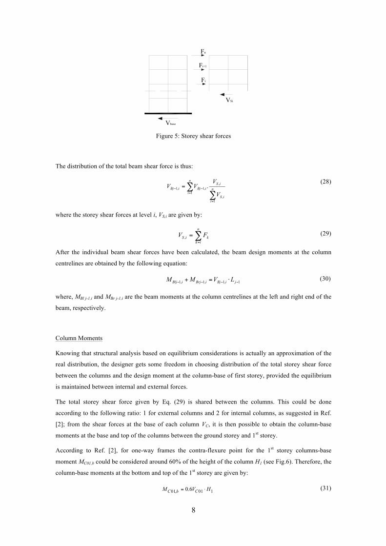
8

Vbase

VSi

Fn

Fi+1

Fi

Figure 5: Storey shear forces

The distribution of the total beam shear force is thus:

∑∑

=

=−− = n

iiS

iSn

iiBjiBj

V

VVV

1,

,

1,1,1 .

(28)

where the storey shear forces at level i, VS,i are given by:

∑=

=n

ikkiS FV ,

(29)

After the individual beam shear forces have been calculated, the beam design moments at the column

centrelines are obtained by the following equation:

1,1,1,1 −−−− ⋅=+ jiBjiBrjiBlj LVMM (30)

where, MBl j-1,i and MBr j-1,i are the beam moments at the column centrelines at the left and right end of the

beam, respectively.

Column Moments

Knowing that structural analysis based on equilibrium considerations is actually an approximation of the

real distribution, the designer gets some freedom in choosing distribution of the total storey shear force

between the columns and the design moment at the column-base of first storey, provided the equilibrium

is maintained between internal and external forces.

The total storey shear force given by Eq. (29) is shared between the columns. This could be done

according to the following ratio: 1 for external columns and 2 for internal columns, as suggested in Ref.

[2]; from the shear forces at the base of each column VC, it is then possible to obtain the column-base

moments at the base and top of the columns between the ground storey and 1st storey.

According to Ref. [2], for one-way frames the contra-flexure point for the 1st storey columns-base

moment MC01,b could be considered around 60% of the height of the column H1 (see Fig.6). Therefore, the

column-base moments at the bottom and top of the 1st storey are given by:

101,01 6.0 HVM CbC ⋅= (31)

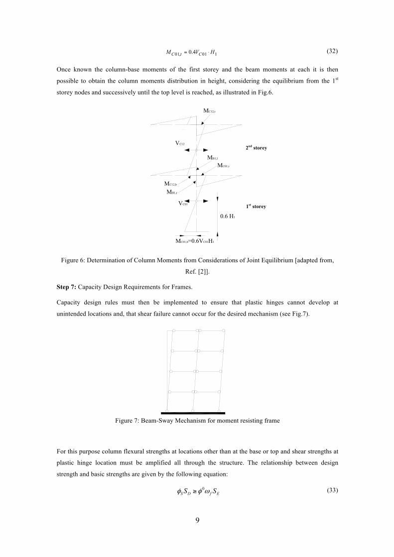
9

101,01 4.0 HVM CtC ⋅= (32)

Once known the column-base moments of the first storey and the beam moments at each it is then

possible to obtain the column moments distribution in height, considering the equilibrium from the 1st

storey nodes and successively until the top level is reached, as illustrated in Fig.6.

MC01,b=0.6VC01H1

VC01

VC12

0.6 H1

MC12,t

MB1,l

MC01,t

MC12,b

MB1,r

Figure 6: Determination of Column Moments from Considerations of Joint Equilibrium [adapted from,

Ref. [2]].

Step 7: Capacity Design Requirements for Frames.

Capacity design rules must then be implemented to ensure that plastic hinges cannot develop at

unintended locations and, that shear failure cannot occur for the desired mechanism (see Fig.7).

Figure 7: Beam-Sway Mechanism for moment resisting frame

For this purpose column flexural strengths at locations other than at the base or top and shear strengths at

plastic hinge location must be amplified all through the structure. The relationship between design

strength and basic strengths are given by the following equation:

EfDS SS ωφφ 0≥ (33)

1st storey

2nd storey

10

where, SD is the design strength defined according to the capacity design rules, φS is a strength reduction

factor relating dependable and design strengths of the action (φS = 1 should be adopted for flexural design

of plastic hinges and φS < 1 for other actions and locations), SE is the basic strength, i.e. the value

corresponding to the design lateral force distribution determined from the DDBD method, φ0 is an

overstrenght factor to account for the overcapacity at the plastic hinges and ωf is the amplification due to

higher mode effects. To apply capacity design rules an approximate method, as proposed in Ref. [2], is

used.

Beam Flexure:

According to the desired inelastic mode, depicted in Fig.7, the plastic hinges should form at beam ends.

For these regions the flexural design of plastic hinges is based on the larger of the moments due to

factored gravity loads or corresponding to the design lateral forces from DDBD procedure (seismic

moments).

For the regions between the beam plastic hinges, design moments are found from the combination of

reduced gravity loads applicable for the seismic design combination, and overstrenght moment capacity at

the beam hinges. Therefore, at a distance x from the left support, the total moment is given by:

( )22

2000,

0,

0,

xwx

LwLxMMMM GG

lErElEx −+×−+= (34)

where L is the beam span, M0E,l (=φ0(x)MBi,l) and M0

E,r (=φ0(x)MBi,l) are the moments at left and right of

column centrelines, respectively, and wG0 is the gravity load (dead and live) constant along the beam and

amplified of 30% of seismic gravity moments are considered to account for elastic vertical response of

the beam to vertical ground accelerations. Eq. (34) is defined taken into account that the beam moments

cannot exceed M0E, the overstrenght values at the beam plastic hinges; thus the design moments are

defined by adding the gravity moments for a simple supported beam to the seismic moments.

Beam Shears:

The seismic beam shears corresponding to the plastic hinges locations are constant along the beam. As

recommended in Ref. [2] the design shear force along the beam, should considerer the effects of beam

vertical response (combined seismic shears with reduced gravity shears applicable for seismic load

combinations), therefore:

( )xw

LwLMM

V GjG

j

lErEx

010

1

0,

0,

2−+

−= −

−

(35)

Column Flexure:

Column end moments, other than at the base or top, and shears forces are amplified for both potential

overstrenght capacity at beam plastic hinges (material strengths exceed the design values) and dynamic

amplification resulting for higher mode effects, which are not considered in the structural analysis.

11

The required column flexural strength according to DDBD capacity design rules is given by:

EfNf MM ωφφ 0≥ (36)

where, φf is the strength reduction factor;

MN is the design column moments;

φ0 is the overstrenght factor;

ωf is the dynamic amplification factor, defined in the following;

ME is the column moments resulting from lateral seismic forces (see Fig.4).

The overstrenght factor φ0 is the ratio of overstrenght moment capacity to required capacity of the plastic

hinges, as referred previously and could be obtained by moment-curvature analysis or using a default

value. The effort to obtain overstrenght factors by moment-curvature analysis maybe excessive for some

structures and as suggested in Ref. [2] a default value should be considered. It is possible to adopt two

values for different situations, if the design is based on a strain-hardening model for the flexural

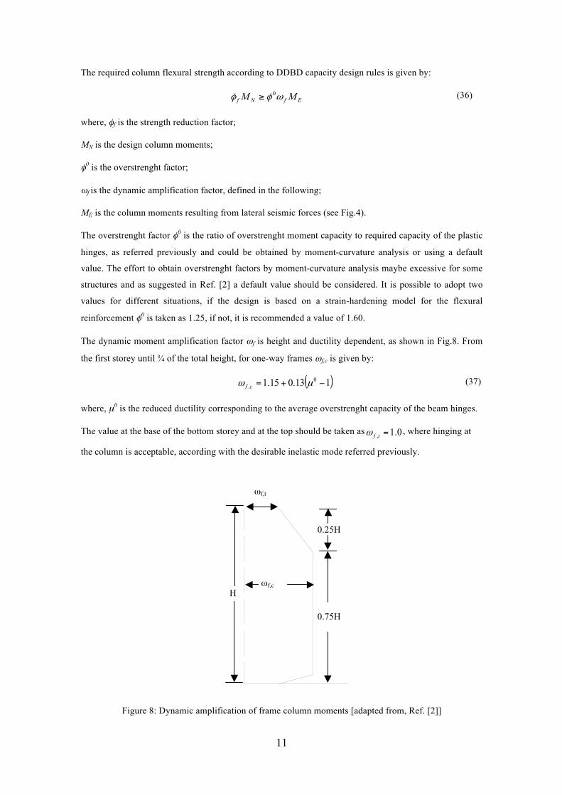
reinforcement φ0 is taken as 1.25, if not, it is recommended a value of 1.60.

The dynamic moment amplification factor ωf is height and ductility dependent, as shown in Fig.8. From

the first storey until ¾ of the total height, for one-way frames ωf,c is given by:

( )113.015.1 0, −+= µω cf

(37)

where, µ0 is the reduced ductility corresponding to the average overstrenght capacity of the beam hinges.

The value at the base of the bottom storey and at the top should be taken as 0.1, =tfω , where hinging at

the column is acceptable, according with the desirable inelastic mode referred previously.

Figure 8: Dynamic amplification of frame column moments [adapted from, Ref. [2]]

0.75H

ωf,c H

0.25H

ωf,t

12

Column Design Shear Forces:

According to Ref. [2] it has been stated that the dynamic amplification factor for column shear should be

obtained by a constant offset of shear demand above design-force envelope with height, given by:

Ci

bCitCibaseEENS H

MMVVV

0,

0,

,0 1.0

+≤+≥ µφφ (38)

where,

VE is the shear demands from lateral seismic forces;

VE, base is the VE value at the base of the column;

µ is the displacement ductility;

MCi,to and MCi,b

o are the moments at the top and bottom of the column, respectively, corresponding to

development of plastic hinging;

Hci is the clear height of the column.

13

3. Case of study- Reinforced Concrete Frame

The DDBD procedure is applied [5, 6] to the interior frame of the four-storey reinforced concrete

structure plotted as section A-A of Fig.9, with a global geometry (height and spans as well as beams and

columns cross-section dimensions) defined in the context of the “Cooperative Research on the Seismic

Response of the Reinforced Concrete Structures” [7]. The structure is irregular in terms of spans and the

lateral resistance is provided by one-way frame action. The slab thickness is equal to 0.15 m. The

reinforced concrete frames are made with concrete C25/30 (fcd = 16.7 MPa). The reinforcement steel is a

classical Tempcore steel B500 (fy =500 MPa). In addition to the self-weight of the beams and the slab, due

to floor finishing and partitions a distributed dead load of 2 kN/m2 is considered, as well as an imposed

live load with nominal value of 2 kN/m2.

Figure 9: General Layout [adapted from, Ref. [7]]

In a first stage, the frame building is designed according to the Direct Displacement Based Design

procedure considering being located in Continental Portugal (Algarve) seismic zone 1.1, as an ordinary

building, class of importance II. The seismic action was defined according to Eurocode 8 [4] and

Portuguese National Annex [8] with the elastic acceleration response spectrum Sa for subsoil class D. The

value of peak ground acceleration ag used in the definition of the response spectrum is 0.35g. The elastic

displacement spectrum SDe used for DDBD, shown in Fig.10, is the one defined in Eurocode 8 by:

2

2)()( !"

#$%

&=πTTSTS aDe

(39)

Figure 10: Design Displacement Spectrum

14

The second stage regards the application of the DDBD procedure when the displacement capacity

exceeds the spectral demand. For this purpose the DDBD procedure was applied again to the same case of

study but considering the building located in Continental Portugal (Lisbon) seismic zone 1.3, for a design

ground acceleration ag of 0.27g.

The seismic performance of the designed structure for peak ground acceleration (ag) of 0.35g was assess

by means of non-linear dynamic analyses and it is presented in Section 3.3.

3.1. Direct Displacement Based Design for a peak ground Acceleration of 0.35g

In this section is presented the frame design according to DDBD procedure and for ag equal to 0.35g. The

step-by-step procedure defined in section 2 is following in this case study.

Step 1: Definition of the design storey displacement, design displacement of the SDOF structure,

equivalent mass and equivalent height

The normalised inelastic mode shape of the MDOF frame structure for this case of study is given by Eq.

(1), with n=4. According to Ref. [2], for frame buildings the design displacement of the substitute SDOF

structure will usually be governed by a specified drift limit in the lower storeys of the building. This

shape implies that the maximum drift occurs between the ground and first storey. For design purpose and

according Ref. [2] the drift limit was considered as 2.5 %. The critical design storey displacement for the

first storey (H1= 3.275 m) is thus Δc = m0818.0275.3025.01 =×=Δ and the critical normalised inelastic

mode shape δc = δ1= 0.267.

The design storey displacement profile is found from Eq. (3), reproduced herein by convenience:

ii

c

ci δδ

δωθ 307.0

267.0082.00.1 =×=%%

&

'(()

* Δ=Δ (40)

where, ωθ is taken as 1.0.

Table 1 presents the calculations to obtain the design displacement of the equivalent SDOF structure and

equivalent height.

Table 1: Calculations to obtain design displacement of the SDOF structure

Storey, i Height, Hi (m) Mass, mi (ton) δi Δi (m) mi Δi mi Δi2 mi Δi Hi

4 12.275 46.59 1.00 0.307 14.30 4.39 175.51 3 9.275 46.59 0.76 0.232 10.80 2.51 100.21 2 6.275 46.59 0.51 0.157 7.31 1.15 45.87 1 3.275 46.95 0.27 0.082 3.84 0.31 12.59 Σ 36.26 8.35 334.18

In Fig.11 is depicted the design storey displacements profile according to the selected target drift limit,

where the top target displacement Δtarget (roof displacement) is equal to 0.307m.

15

Figure 11: Design storey displacements

From Eq. (4) to Eq. (6) and from the values presented in Table 1 it is possible to derive the design

displacement Δd, the equivalent mass me and equivalent height He of the SDOF structure. Therefore, the

design displacement of the SDOF structure is 0.23m, the equivalent mass is 157.34 tonne and the

equivalent height is 9.217m (75.1% of building height).

Step 2: Estimation of the level of equivalent viscous damping

The design displacement ductility is given by Eq. (7), reproduced herein by convenience:

y

d

Δ

Δ=µ (41)

The equivalent yield displacement is the product between the yield rotation (see Eq. (9)) and the

equivalent height of the SDOF structure. In this case of study, with beam depths for spans 1 and 2 hb1 =

hb2 = 450 mm, the yield rotation θy is given by:

ib

yiy hL,1

1,1 5.0 εθ ×= (42)

ib

ibyiy hL

,2

,2,2 5.0 εθ ×= (43)

The yield strain is thus:

00275.02000005001.1 =×== syey Efε (44)

where the design yield strength of steel is fye = 1.1 fy, according to the recommendations in Ref. [2] for

design material strengths for plastic hinge regions.

The equivalent yield displacement is given by:

mHMMMM

eii

iyiiyiy 141.0217.9

2012.0018.0

,2,1

,2,2,1,1 =×+

=⋅+

+=Δ

θθ (45)

16

The M1,i and M2,i are the contribution from both bays, and the considered relationship between them is

M1,i/ M2,i = 1.

Replacing in Eq. (41) the design displacement of the SDOF structure and the equivalent yield

displacement, the SDOF system design displacement ductility is µ=1.64.

The equivalent viscous damping of the SDOF structure was obtained by Eq. (10), reproduced herein by

convenience:

%99.111565.005.0 =!!"

#$$%

& −+=

µπµ

ξ (46)

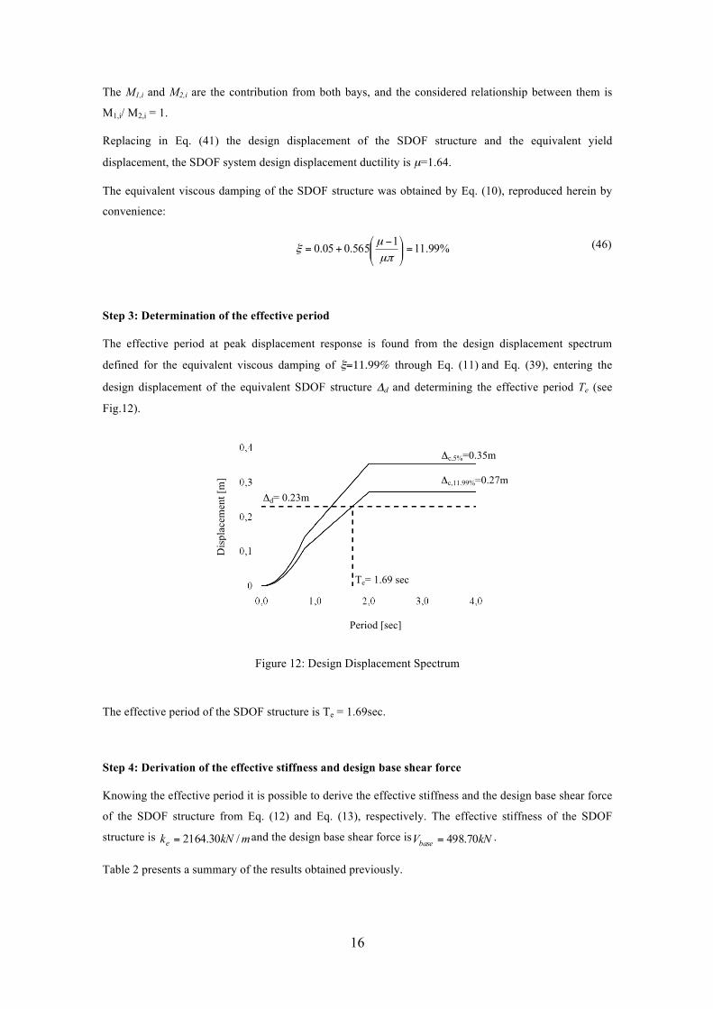
Step 3: Determination of the effective period

The effective period at peak displacement response is found from the design displacement spectrum

defined for the equivalent viscous damping of ξ=11.99% through Eq. (11) and Eq. (39), entering the

design displacement of the equivalent SDOF structure Δd and determining the effective period Te (see

Fig.12).


The effective period of the SDOF structure is Te = 1.69sec.

Step 4: Derivation of the effective stiffness and design base shear force

Knowing the effective period it is possible to derive the effective stiffness and the design base shear force

of the SDOF structure from Eq. (12) and Eq. (13), respectively. The effective stiffness of the SDOF

structure is mkNke /30.2164= and the design base shear force is kNVbase 70.498= .

Table 2 presents a summary of the results obtained previously.

Period [sec]

Dis

plac

emen

t [m

]

Te= 1.69 sec

Δc,5%=0.35m

Δc,11.99%=0.27m

Δd= 0.23m

17

Table 2: Results of DDBD in terms of displacement, equivalent yield displacement, ductility, effective

mass, effective period and design base shear force

Δtarget (m) Δd (m) Δy (m) µ me (tonne) ξ (%) Te (s) Vbase (kN) 0.307 0.230 0.141 1.64 157.34 11.99 1.69 498.70

Step 5: Distribution of the design base shear force

The next step of the DDBD procedure involves the distribution of the design base shear force obtained for

the SDOF structure in the real structure (MDOF structure), in a variation of the equivalent lateral force-

based. The distribution of the design base shear through the real structure was obtained by Eq. (17) and

the values presented in Table 3.

Step 6: Design actions for MDOF Structure

The real structure is then analyzed under these forces (defined in step 5) and then the design moments are

obtained.

Beam Moments

Table 3 shows the calculations to obtain the distribution of the design base shear through the real

structures, the value of column shear forces in each alignment (shared between the exterior and interior

columns in proportion 1:2 as suggested in Ref. [2]). Storey shear forces VSi obtained from Eq. (29) are

defined by summing the storey shear forces above the storey (see Fig.5). The last column of Table 3

presents the overturning moment OTM given by Eq. (20).

Table 3: Calculations

Storey, i Height, Hi (m) miΔi Fi (kN) VCi,1

Col 1 (kN) VCi,2

Col 2 (kN) VCi,3

Col 3 (kN) VS,i (kN) OTM (kNm)

4 12.275 14.30 196.69 49.17 98.34 49.17 196.69 0 3 9.275 10.80 148.62 37.15 74.31 37.15 345.30 590.06 2 6.275 7.31 100.55 25.14 50.27 25.14 445.85 1625.96 1 3.275 3.84 52.88 13.22 26.44 13.22 498.73 2963.49 0 0 0.00 0.00 0.00 4596.82

Sum 36.26 498.73 124.68 249.36 124.68 1486.56

- P-Δ!effects

According to Eq. (14) the stability index θΔ for this example is 0.094, therefore there is no need to consider

P-Δ effects, because θΔ < 0.10.

Thus, the value of the design base shear force Vbase to use in DDBD procedure is 498.73kN and the values

presented in Table 3 are used in further calculations.

Based on Eq. (31) the total resisting moment provided at the column base is thus:

∑ =××== kNmVHM basecj 0.980275.36.07.4986.0 1 (≈ 21.3% OTM) (47)

18

According to Eq. (27), beam seismic shears corresponding to design lateral forces, admitting a

relationship between beam moments MB1,i/MB2,i=1, for span 1 and 2, respectively, are given by:

( ) kNVn

iiB 4.3016/0.9808.459621

1,1 =−=∑

=

(48)

( ) kNVn

iiB 1.4524/0.9804596.821

1,2 =−=∑

=

(49)

These forces are distributed to the beams in proportion to the storey shears directly below the beams

considered according to Eq. (28) and Eq. (29).

iSiSiB VVV ,,,1 203.056.1486/4.301 =×= (50)

iSiSiB VVV ,,,2 304.056.1486/1.452 =×= (51)

The resulting seismic beam shears for each span is presented in Table 4.

Table 4: Calculations for seismic beam shears

Storey, i VB1,i (kN) VB2,i (kN) 4 39,90 59,80 3 70,00 105,00 2 90,40 135,60 1 101,10 151,70

The beam design moments at the column centrelines are given by Eq. (30) and at column faces by:

( ) 2/1,1,1 cjiBjiBj hLVM −= −−− (52)

In Tables 5 and 6 are presented the values of the seismic design beam moments at the centreline and at

the column face, respectively.

Table 5: Beam seismic moments at the centreline (ignoring gravity loads)

Span 1 (L1=6m) Span 2 (L2=4m) Storey, i MB1,i.l (kNm) MB1,i,r (kNm) MB2,i,l (kNm) MB2,i,r (kNm)

4 119.63 119.63 119.63 119.63 3 210.03 210.03 210.03 210.03 2 271.19 271.19 271.19 271.19 1 303.35 303.35 303.35 303.35

Table 6: Beam seismic moments at the face of the column (ignoring gravity loads)

Span 1 (L1=6m) Span 2 (L2=4m) Storey, i MB1,i.l (kNm) MB1,i,r (kNm) MB2,i,l (kNm) MB2,i,r (kNm)

4 111.66 -110.66 106.18 -107.67 3 196.03 -194.28 186.40 -189.03 2 253.11 -250.85 240.68 -244.07 1 283.13 -280.60 269.23 -273.02

According to Ref. [2] the flexural design of the beam plastic hinges is based on moments due to factored

gravity loads or seismic moments corresponding to the design lateral forces (seismic case). Both values

19

should be compared and the larger should be adopted for the design. Therefore, it is presented the

calculations for these two cases. The factored gravity moments were obtained considered three load cases:

1) the dead and live loads applied to both spans at the same time, 2) and 3) considering alternate live

loads acting in the spans. Fig.13 shows the larger beam moment from these three combinations.

Figure 13: Beam moment distribution due to factored gravity loads [units in kNm]

In Table 7 is presented the larger beam factored gravity moments for the three combinations.

Table 7: Beam moments due to factored-gravity loads [units in kNm]

Storey, i Span 1 Span 2 left end mid span right end left end mid span right end

4 153.38 129.57 212.52 128.03 46.55 59.82 3 191.91 114.96 205.11 94.06 47.24 87.12 2 184.85 114.96 207.73 102.23 47.00 80.31 1 175.07 118.32 212.31 112.56 46.73 70.50

The beam ends (plastic hinge locations) should be designed for the larger of the moments presented in

Table 6 and 7, respectively. In Table 8 is shown the design beam moments for plastic hinges locations;

the moments bold marked is due to factored gravity loads.

Table 8: Design beam moments [units in kNm]

Storey, i Span 1 Span 2 left end right end left end right end

4 153.38 212,52 128.03 -107.67 3 196.03 205.11 186.40 -189.03 2 253.11 250.85 240.68 -244.07 1 283.13 280.60 269.23 -273.02

212.31

207.73

205.11

212.52.

94.06

102.23

112.56

20

Column moments

The column moments presented in Table 9 corresponds to the design lateral forces and they were

obtained by equilibrium considerations as described previously in section 2.

Table 9: Column moments [units in kNm]

Storey, i Col 1 Col 2 Col 3

4 Top 119.63 239.30 119.63 bottom -27.90 -55.80 -27.90

3 Top 182.15 364.30 182.15 bottom -76.82 -153.64 -76.82

2 Top 194.40 388.72 194.40 bottom -140.02 -280.03 -140.02

1 Top 163.33 326.70 163.33 bottom -245.00 -490.00 -245.00

Step 7: Capacity design requirements for frames

In the following it is presented the application of the capacity design rules.

Beam Flexure

In DDBD procedure recommendations [2] the material design strengths for design locations of intended

plastic hinges, for concrete and reinforcement should be fće=1.3fć and fye =1.1fy, respectively. Where, f’c

is the specified (28 days) concrete compression strength, fće is the expected compression strength of

DDBD, f’y is the specified minimum characteristic yield strength of steel and fye is the expected yield

strength of steel for DDBD.

Thus, for a concrete C25/30 and reinforcement steel B500 the following values will apply:

• Concrete compression

MPafce 5.32253.1' =×= !! ! ! (53)!!!!!!!!!!!!!!!!!!!!!!!!!!!!!!!!!!!!!!!!!!!!!!!!

( )]10[5.17.21'

=== cc

cecd MPaff γ

γ (54)

MPaff cectm 3'30.0 )3/2( == (55)

!• Steel reinforcement

MPaf ye 5505001.1 =×= (56)

( )]10[15.15.478 === ss

yeyd MPa

ff γ

γ (57)

The required longitudinal reinforcement for beams ends is shown in Table 10. The longitudinal

reinforcement was obtained for simple flexure; the values of Table 8 are reproduced for convenience.

21

Table 10: Longitudinal reinforcement for beam plastic hinges (tension zone)

Design details:

b= 0.30m; d=0.42m b=width; d=effective depth

Storey, i Location Msd (kNm) µ ω As(cm2) φ Asprovided(cm2) ρ!(%)!

Span 1

1 left end 283.13 0.247 0.290 16.60 9φ16 18.10 1.44

right end 280.60 0.245 0.287 16.38 9φ16 18.10 1.44

2 left end 253.11 0.221 0.254 14.50 8φ16 16.08 1.28

right end 250.85 0.219 0.251 14.34 8φ16 16.08 1.28

3 left end 196.03 0.171 0.189 10.80 6φ16 12.06 0.96

right end 205.11 0.178 0.200 9.95 6φ16 12.06 0.96

4 left end 153.38 0.134 0.145 8.30 6φ16 12.06 0.96

right end 212.52 0.185 0.207 10.30 6φ16 12.06 0.96

Span 2

1 left end 269.23 0.235 0.273 15.57 8φ16 16.08 1.28

right end 273.02 0.238 0.277 15.83 8φ16 16.08 1.28

2 left end 240.68 0.210 0.239 13.64 8φ16 16.08 1.28

right end 244.07 0.213 0.243 13.90 8φ16 16.08 1.28

3 left end 186.40 0.163 0.179 10.22 6φ16 12.06 0.96

right end 189.03 0.165 0.181 10.40 6φ16 12.06 0.96

4 left end 128.03 0.112 0.119 6.80 6φ16 12.06 0.96

right end 107.67 0.094 0.100 5.70 6φ16 12.06 0.96

The reinforcement values for beams were obtained considering the requests specified in Eurocode 8 [4]

for Ductility Class Medium (DCM) structures at plastic hinges locations. To verify the local ductility

conditions according to EC8, the following requirements must be fulfilled:

• The value of the curvature ductility factor µφ shall be at least equal to:

CTTifq ≥−= 10 12φµ (58)

CTTifq <−+= 10 )1(21φµ (59)

in this case of study, ( )3513212 00 ==−×=−= qqφµ

• In the compression zone, reinforcement should be at least half of the reinforcement provided in

the tension, in addition to any compression reinforcement needed for the ULS verification of the

beam in the seismic design situation.

• The reinforcement ratio of the tension zone ρ does not exceed a value!ρmax equal to:!

%68.0´105.4780024.05

107.210018.0'.0018.0' 3

3

,max +=

×××××

+=+= ρρεµ

ρρφ yd

cd

yds ff

(60)

where,!ρ’!is the reinforcement ratio of the compression zone and εs, yd = 0.0024

!For this case of study the reinforcement of the compression zone will be equal to the reinforcement of the

tension zone.

Through the entire length of a primary seismic beam the reinforcement ratio of the tension zone!ρ shall be

not less than the following minimum value:!!

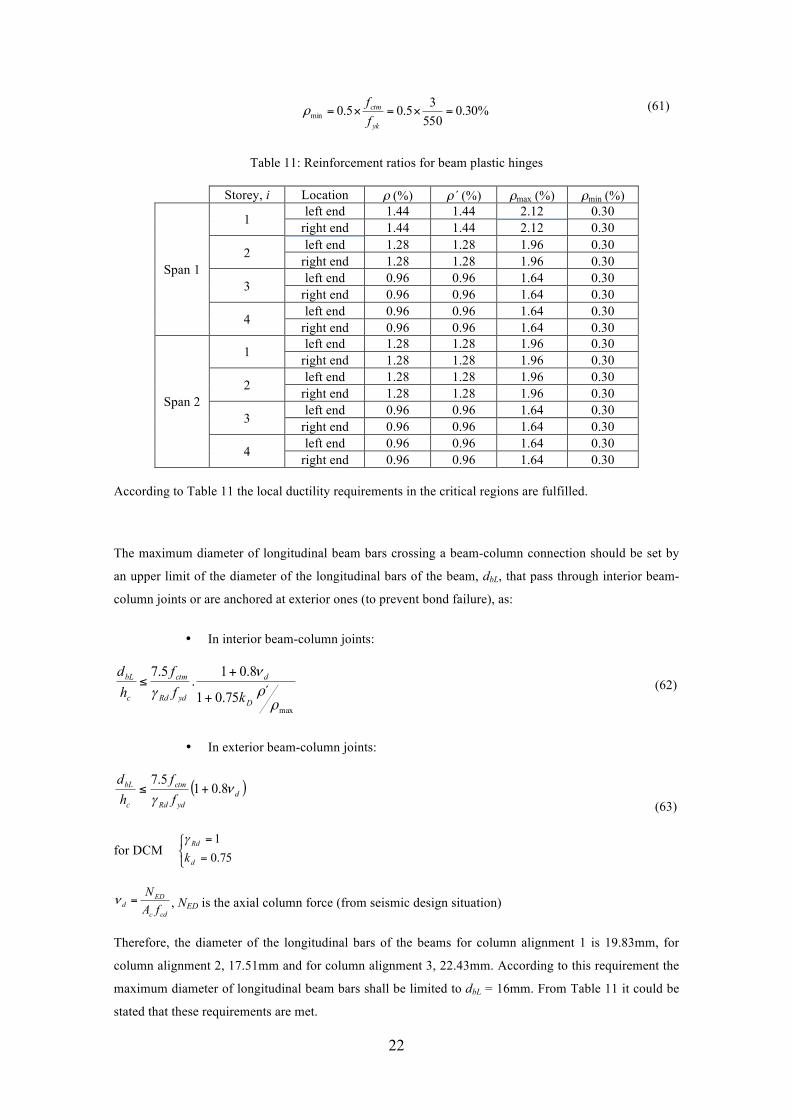
22

!!!!!!!!!!!!!!!!!!!!!!! !!!!!!!!!!!!!!!%30.0

55035.05.0min =×=×=

yk

ctm

ff

ρ!

(61)

Table 11: Reinforcement ratios for beam plastic hinges

Storey, i Location ρ!(%)! ρ´ (%) ρmax (%) ρmin!(%)

Span 1

1 left end 1.44 1.44 2.12 0.30 right end 1.44 1.44 2.12 0.30




Span 2





According to Table 11 the local ductility requirements in the critical regions are fulfilled.

The maximum diameter of longitudinal beam bars crossing a beam-column connection should be set by

an upper limit of the diameter of the longitudinal bars of the beam, dbL, that pass through interior beam-

column joints or are anchored at exterior ones (to prevent bond failure), as:

• In interior beam-column joints:

max

´75.01

8.01.

5.7

ρρν

γD

d

ydRd

ctm

c

bL

kff

hd

+

+≤ (62)

• In exterior beam-column joints:

( )dydRd

ctm

c

bL

ff

hd

νγ

8.015.7

+≤ (63)

for DCM !"#

=

=

75.01

d

Rd

kγ

cdc

EDd fA

N=ν , NED is the axial column force (from seismic design situation)

Therefore, the diameter of the longitudinal bars of the beams for column alignment 1 is 19.83mm, for

column alignment 2, 17.51mm and for column alignment 3, 22.43mm. According to this requirement the

maximum diameter of longitudinal beam bars shall be limited to dbL = 16mm. From Table 11 it could be

stated that these requirements are met.

23

The design beam moments at mid span due to seismic loads are given in Table 12 and the correspondent

beam longitudinal reinforcement at Table 13. These are obtained from the combination of reduced gravity

loads applicable for the design seismic combination, and overstrenght moment capacity at beam hinge

location, according to Eq. (34). The overstrenght factor φ0 is considered equal to 1.25. The design material

strengths used are the characteristic material strengths, without amplification.

Table 12: Design beam moments at mid span [units in kNm]

Storey, i Span 1 Span 2

4 216.16 214.60 3 216.63 213.89

2 216.95 213.42

1 217.11 213.16

Table 13: Beam longitudinal reinforcement for mid span

Design details:

Concrete C25/30 b= 0.30m; d=0.42m

Steel: A500 NR b=width; d= effective depth

Storey, i Msd (kNm)! µ ω As(cm2) φ As provided(cm2) ρ!(%)

Span 1

1 217.11 0.246 0.288 13.96 7φ16 14.07 1.12 2 216.95 0.245 0.288 13.96 7φ16 14.07 1.12 3 216.63 0.245 0.288 13.96 7φ16 14.07 1.12 4 216.16 0.244 0.287 13.88 7φ16 14.07 1.12

Span 2

1 213.16 0.241 0.282 13.63 7φ16 14.07 1.12 2 213.42 0.241 0.282 13.63 7φ16 14.07 1.12 3 213.89 0.242 0.283 13.70 7φ16 14.07 1.12 4 214.60 0.243 0.284 13.75 7φ16 14.07 1.12

Column Flexure

The required column flexural strength according to DDBD capacity design rules is given by Eq. (36),

reproduced herein by convenience.

EfNf MM ωφφ 0≥ (64)!

φ0 is the overstrenght factor considered as 1.25;

ωf is the dynamic amplification factor - Eq. (37);

ME is the column moments resulting from design forces (given in Table 9);

φf is the strength reduction factor considered as 0.9.

The design column moments and axial forces are shown in Table 14 and 15, respectively. Fig.14 presents

a scheme of the design column moments.

24

Table 14: Design column moments [units in kNm]

Storey , i Location ωf Col 1 Col 2 Col 3

4 Top 1 166.15 332.31 166.15

bottom 1 -45.92 -91.84 -45.92

3 Top 1.190 300.02 600.03 300.02 bottom 1.190 -126.99 -253.98 -126.99

2 Top 1.186 321.28 642.56 321.28

bottom 1.186 -231.45 -462.90 -231.45

1 Top 1 269.99 539.97 269.99 bottom 1 -306.24 -612.50 -306.24

-306.24

-231.45

-127.00

-45.92 -91.84

-253.98

-462.90

-612.50 -306.24

-45.92

-127.00

-231.45

166.15

270.00

321.28

300.02

332.31 166.15

300.02600.03

321.28642.56

539.97270.00

Figure 14: Design column moments distribution [units in kNm]

Table 15: Axial forces in columns [units in kN]

Storey, i Location Col 1 Col 2 Col 3

4 Top -99.90 -213.03 -153.00 bottom -99.90 -213.03 -153.00

3 Top -169.68 -410.99 -351.20 bottom -169.68 -410.99 -351.20

2 Top -219.06 -598.77 -579.98 bottom -219.06 -598.77 -579.98

1 Top -258.81 -782.97 -825.56

bottom -258.81 -782.97 -825.56

The required longitudinal reinforcement for the rectangular column sections was obtained considering

composed bending and it is presented in Table 16. The required longitudinal reinforcement was obtained

using simplified equations for rectangular cross sections with symmetric reinforcement [9]. The recover

rebar was considered as 3 cm.

The design material design strengths used are the characteristic ones, without amplification, except for the

column base, where it is expected the formation of plastic hinges (beam-sway mechanism).

25

Table 16: Longitudinal reinforcement bars /face

Design details:

Concrete C25/30 exterior col. b= 0.40m;h=0.40m

Steel: A500 NR interior col. b= 0.45m;h=0.45m Storey, i Col 1 Col 2 Col 3

4 3φ25 (14.73cm2)

3φ32 (24.13cm2)

3φ25 (14.73cm2)

3 4φ25 (19.63cm2)

4φ32 (32.17cm2)

4φ25 (19.63cm2)

2 4φ25 (19.63cm2)

4φ32 (32.17cm2)

4φ25 (19.63cm2)

1 4φ25 (19.63cm2)

4φ32 (32.17cm2)

4φ25 (19.63cm2)

Table 17: Reinforcement ratios (ρ (%))

Storey, i Col 1 (Ac=0.16m2)

Col 2 (Ac=0.2025m2)

Col 3 (Ac=0.16m2)

4 1.84 2.38 1.84 3 2.45 3.18 2.45 2 2.45 3.18 2.45 1 2.45 3.18 2.45

According to EC8 for a structure with a class ductility medium (DCM) the longitudinal reinforcement

ratio for columns should be greater than 0.01 (1%) and not less of 0.04 (4%). From Table 17 it can be

stated that these requirement are fulfilled.

3.2. Direct Displacement Based Design for a peak ground acceleration of 0.27g

The DDBD procedure is applied again to the same frame with the objective of illustrating the design

situation when the displacement capacity exceeds the maximum possible spectral displacement demand.

In this situation, the building was considered being located in Continental Portugal (Lisbon) seismic zone

1.3, as an ordinary building, class of importance II. The value of the peak ground acceleration ag used in

the definition of the response spectrum is 0.27g. Some of the results were obtained previously in section

3.1 and are herein reproduced for convenience. In Table 18 is presented a summary of the results obtained

previously from the DDBD procedure, steps 1 and 2.

Table 18: Results of DDBD in terms of design displacement, equivalent yield displacement, ductility,

effective mass and equivalent viscous damping

Δtarget (m) Δd (m) Δy (m) µ me (tonne) ξ (%) 0.307 0.230 0.141 1.64 157.34 11.99

26

The step 3 of the DDBD procedure involves the determination of the effective period at peak

displacement response and it is found from the design displacement spectrum as referred in section 3.1

(see Fig.15).


From Fig.15 it can be observed that the design displacement capacity for the SDOF structure exceeds the

maximum possible spectral displacement demand for the considered damping level. This design situation

can occur for very tall or flexible structures or when peak ground acceleration is too low. For these cases

two possibilities must be considered: a) equivalent yield displacement may exceed 5% damping corner

displacement, or b) equivalent yield displacement is less than 5% damping corner displacement, see

Fig.16 a) and b), respectively.

a) Δy> Δc,5% b) Δy< Δc,5%

Figure 16: Design situations when the displacement capacity exceeds the spectral demand

a) Yield displacement exceeds 5% damping value at the period corner (Δy > Δc,5%)

The structure will respond elastically and the response period Tel will be larger than the corner period

TD ( )Del TT > . As suggested in Ref. [2] the response displacement will be taken equal to %5,cΔ , thus the

required design base shear force is given by:

%5,celbase kV Δ×= (65)

ΔC,5%=0.27m

ΔC,11.99%=0.21m

Δd= 0.23m

Δd

Δc,5%

Δy

Δc,ξ

Δc,5%

Δc,ξ

Δd

Δy

27

where, kel is the elastic stiffness and %5,cΔ is the 5% damping elastic response displacement.

In this design situation the solution is not unique. In fact the stiffness kel depends on the elastic period,

which depends in turn, on the strength. This leads to an uncertainty in choosing an acceptable value for

the strength. Minimum strength requirements for P-Δ effects or gravity loads will governs the required

strength.

b) Yield displacement is less than 5% damping value at the period corner (Δy < Δc,5%) An inelastic response will occur but not at the level of ductility corresponding to the displacement or drift

capacity of the structure. As in the previous case there was not a unique solution and elastic stiffness

could correspond to any period larger than the period corner. Herein, the elastic period Tel is taken with

the value of the period corner TD, because if Tel is less than TD the displacement capacity value will be

incompatible with equivalent damping. An iterative method is required and the following procedure is

recommended in Ref. [2]:

a. Calculate displacement capacity, Δd, and the corresponding damping ξ.

b. Calculate approximately the final displacement response Δdf (one possibility to a first guess is to

consider Δdf = (Δc,ξ+ Δd)/2).

c. Calculate the displacement ductility demand corresponding to Δdf (µ =Δdf/Δy).

d. Calculate the damping ξ corresponding to ductility demand µ.

e. Calculate the displacement response Δc,ξ at TD corresponding to ξ.

f. Use this new value Δc,ξ as a new estimation of the final displacement Δdf, iteratively.

g. Cycle trough steps c. to f. until a stable solution it found.

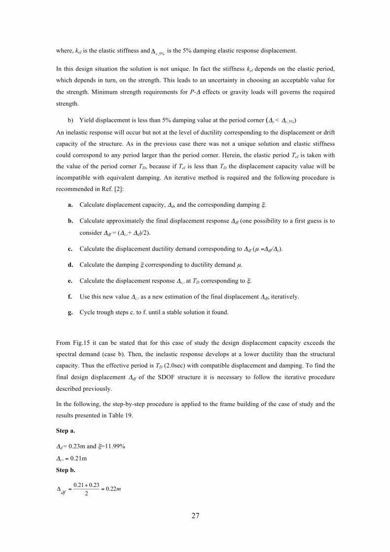
From Fig.15 it can be stated that for this case of study the design displacement capacity exceeds the

spectral demand (case b). Then, the inelastic response develops at a lower ductility than the structural

capacity. Thus the effective period is TD (2.0sec) with compatible displacement and damping. To find the

final design displacement Δdf of the SDOF structure it is necessary to follow the iterative procedure

described previously.

In the following, the step-by-step procedure is applied to the frame building of the case of study and the

results presented in Table 19.

Step a.

Δd = 0.23m and ξ=11.99%

Δc,ξ = 0.21m

Step b.

mdf

22.0223.021.0

=+

=Δ

28

Step c.

56.114.022.0

==Δ

Δ=

y

dfµ

Step d.

%47.1110 =!!

"

#$$%

& −+=

µπµ

ξξhyst

Step e.

m213.047.115

1027.05.0

)47.11,2( =!"

#$%

&+

=Δ

This will be a new estimate for the final displacement.

Step f.

go to step c. to f. until a stable solution is found (see Table 19).

Table 19: Iterative procedure results

Δdf (m) µ ξ (%) Δ(c.ξ) (m) 1º 0.220 1.57 11.47 0.213 2º 0.213 1.51 11.10 0.216 3º 0.216 1.53 11.23 0.215 4º 0.215 1.52 11.18 0.215

The final design displacement of the SDOF structure is 0.215m.

Fig.17 shows the design displacement spectrum for 5% damping and for the initial damping (ξ=11.99%),

as the initial (Δd = 0.230m) and final displacement response (Δdf = 0.215m).


The design base shear force is thus:

kNTmkVD

edeldbase 87.3334

2

2

=×Δ=×Δ=π (66)

Any value less than Vbase will satisfy the design assumption.

Te=TD=2.0sec

Δd=0.230m

Δc,5%=0.270m

Δdf=0.215m Δc,11.99%=0.210m

29

4. Final remarks

In this report has been presented a brief summary of the Direct Displacement Based Design (DDBD)

procedure. This design procedure was applied to a simple case of study, a reinforced concrete frame

building. Different seismic intensities were considered: peak ground accelerations of 0.35g and 0.27g

were adopted. For the peak ground acceleration of 0.35g, the design displacement capacity of the frame

structure obtained through the DDBD procedure is less than the maximum possible spectral displacement

demand for the considered damping level. For the low seismicity case (0.27g) the displacement capacity

exceeds the maximum possible spectral displacement demand.

It can be stated that the DDBD procedure leads to an easy design than the traditional force-based

procedures [3]. However, the DDBD procedure is based on hand calculations and throughout the design

process some design choices must be done based on engineering judgment. Moreover, the DDBD

procedure can be more difficult to apply, becoming an iterative procedure in some cases (for very flexible

structures or/and low seismic intensity - see section 3.2). Thus, it is herein suggested to develop an

automatic program.

30

5. References

[1] Priestley, M.N.J. and Kowalsky, M.J. (2000) “Direct Displacement-Based Seismic Design of

Concrete Buildings”, Bulletin of the New Zealand National Society for Earthquake Engineering,

Vol. 44(2). 145–165

[2] Priestley, M.N.J., Calvi, G.M. and Kowalsky, M.J. (2007) “Displacement-Based Seismic Design

of Structures”, IUSS Press, Pavia, Italy

[3] Powell, G.H. (2008) “Displacement-Based Seismic Design of Structures – Book Review”,

Earthquake Spectra, Vol.24. No.2

[4] EN 1998-1:2004 “Eurocode 8: Design of Structures for Earthquake Resistance - Part 1: General

Rules, Seismic Actions and Rules for Buildings”, CEN, Brussels, Belgium.

[5] Massena, B., Degée, H. and Bento, R. (2010) “Consequences of design choices in Direct

Displacement Based Design of RC frames”, 14th ECEE, Ohrid, Republic of Macedonia

[6] Massena, B., Bento, R. and Degée, H. (2010) “Implications of different design assumptions in

Direct Displacement Based Design of RC frames”, Sísmica 2010, Aveiro (Portugal).

[7] CRSRRCS 1992, Negro, P. Varzeletti, G., Magonette, G. E. and Pinto, A., V. (1995) “Tests on the

Four-Storey Full Scale Reinforced Concrete Frame with Masonry Infills: Preliminary Report”,

Joint Research Centre- Ispra, Italy

[8] NP EN 1998-1:2007, “Portuguese National Annex”

[9] D’Arga e Lima J. Monteiro and V. Mun M. (1996) “Betão Armado - Esforços Normais e de

Flexão”, LNEC, Lisboa, Portugal

Documents

direct displacement based design(DDBD)