DIRECT AND ITERATIVE METHODS

FOR BLOCK TRIDIAGONAL LINEAR SYSTEMS

Don Eric Heller

April 1977

Department of Computer Science

Carnegie-Mellon University

Pittsburgh, PA 15213

Submitted in partial fulfillment of the requirements for the degree

of Doctor of Philosophy at Carnegie-Mellon University.

This research was supported in part by the Office of Naval Research

under Contract N00014-76-C-0370, NR 044-422, by the National Science

Foundation under Grant MCS75-222-55, and by the National Aeronautics

and Space Administration under Grant NGR-47-102-001, while the author

was in residence at ICASE, NASA Langley Research Center.

ABSTRACT

Block tridiagonal systems of linear equations occur frequently in

scientific computations, often forming the core of more complicated prob-

lems. Numerical methods for solution of such systems are studied with

emphasis on efficient methods for a vector computer. A convergence theory

for direct methods under conditions of block diagonal dominance is developed,

demonstrating stability, convergence and approximation properties of direct

methods. Block elimination (LU factorization) is linear, cyclic odd-even

reduction is quadratic, and higher-order methods exist. The odd-even

methods are variations of the quadratic Newton iteration for the inverse

matrix, and are the only quadratic methods within a certain reasonable

class of algorithms. Semi-direct methods based on the quadratic conver-

gence of odd-even reduction prove useful in combination with linear itera-

tions for an approximate solution. An execution time analysis for a pipe-

line computer is given, with attention to storage requirements and the

effect of machine constraints on vector operations.

PREFACE

It is with many thanks that I acknowledge Professor J. F. Traub, for

my introduction to numerical mathematics and parallel computation, and for

his support and encouragement. Enlightening conversations with G. J. Fix,

S. H. Fuller, H. T. Kung and D. K. Stevenson have contributed to some of

the ideas presented in the thesis. A number of early results were obtained

while in residence at ICASE, NASA Langley Research Center; J. M. Ortega and

R. G. Voigt were most helpful in clarifying these results. The thesis was

completed while at the Pennsylvania State University, and P. C. Fischer

must be thanked for his forbearance.

Of course, the most important contribution has been that of my wife,

Molly, who has put up with more than her fair share.

ii

CONTENTS

pageI. Introduction .......................... I

A. Summary of Main Results ................... 5

B. Notation .......................... 8

2. Some Initial Remarks ...................... I0

A. Analytic Tools ....................... I0

B. Models of Parallel Computation ............... 14

3. Linear Methods ......................... 18

A. The LU Factorization .................... 18

I. Block Elimination .................... 18

2. Further Properties of Block Elimination ......... 25

3. Back Substitution .................... 30

4. Special Techniques ................... 31

B. Gauss-Jordan Elimination .................. 33

C. Parallel Computation .................... 36

4. Quadratic Methods ........................ 37

A. Odd-Even Elimination .................... 37

B. Variants of Odd-Even Elimination .............. 45

C. Odd-Even Reduction ..................... 48

I. The Basic Algorithm ................... 48

2. Relation to Block Elimination .............. 51

3. Back Substitution .................... 56

4. Storage Requirements .................. 58

5. Special Techniques ................... 59

D. Parallel Computation .................... 60

E. Summary ........................... 64

5. Unification: Iteration and Fill- In ............... 65

iii

6. Higher-Order Methods ....................... 71

A. p-Fold Reduction ....................... 71

B. Convergence Rates ....................... 75

C. Back Substitution ....................... 80

7. Semidirect Methods ........................ 83

A. Incomplete Elimination .................... 84

B. Incomplete Reduction ..................... 86

C. Applicability of the Methods ................. 90

8. Iterative Methods ......................... 92

A. Use of Elimination ...................... 92

B. Splittings .......................... 93

C. Multi- line Orderings ..................... 94

D. Spiral Orderings ....................... 97

E. Parallel Gauss ........................ I01

9. Applications .......................... 105

A. Curve Fitting ......................... 105

B. Finite Elements ........................ 106

I0. Implementation of Algorithms ................... Ii0

A. Choice of Algorithms (Generalities). ............. II0

B. Storage Requirements ..................... 113

C. Comparative Timing Analysis .................. 120

Appendix A. Vector Computer Instructions ............... 131

Appendix B. Summary of Algorithms and Timings ............ 136

References .............................. 156

iv

I. INTRODUCT ION

Block tridiagonal matrices are a special class of matrices which arise

in a variety of scientific and engineering computations, typically in the

numerical solution of differential equations. For now it is sufficient to

say that the matrix looks like

bI cI2 b2 c2

a3 b3 c3A _ • • • ,

aN-I bN-I _-I

aN bN/

where b is an n X n matrix and a c are dimensioned conformaIly• Thusi i i N i' i N

nj) × ( nj).the full matrix A has dimension (_j=l

In this thesis we study numerical methods for solution of a block tri-

diagonal linear system Ax = v, with emphasis on efficient methods for a

vector-oriented parallel computer (e.g., CDC STAR-100, llliac IV). Our

analysis primarily concerns numerical properties of the algorithms, with

discussion of their inherent parallelism and areas of application• For

this reason many of our results also apply to standard sequential algo-

rithms. A unifying analytic theme is that a wide variety of direct and

iterative methods can be viewed as special cases of a general matrix itera-

tion, and we make considerable use of a convergence theory for direct

methods. Algorithms are compared using execution time estimates for a

simplified model of the CDC STAR-100 and recommendations are made on this

basis.

There are two important subclasses of block tridiagonal matrices,

depending on whether the blocks are small and dense or large and sparse.

A computational method to solve the linear system Ax = v should take

into account the internal structure of the blocks in order to obtain

storage economy and a low operation count. Moreover, there are impor-

tant applications in which an approximate solution is satisfactory.

Such considerations often motivate iterative methods for large sparse

systems, especially when a direct method would be far more expensive.

Since 1965, however, there has been an increased interest in the

direct solution of special systems derived from two-dimenslonal elliptic

partial differential equations. With a standard five-point finite differ-

ence approximation on a rectangular grid, the ai, ci blocks are diagonal

and the b. blocks are tridiagonal, so A possesses a very regular sparsei

structure. By further specializing the differential equation more struc-

ture will be available. Indeed, the seminal paper for many of the impor-

tant developments dealt with the simplest possible elliptic equation. This

was Hockney's work [H5], based on an original suggestion by Golub, on the

use of Fourier transforms and the cyclic reduction algorithm for the solu-

tion of Poisson's equation on a rectangle. For an n X n square grid Hockney

was able to solve Ax = v in O(n 3) arithmetic operations, while ordinary band-

matrix methods required O(#) operations. Other O(n 3) methods for Poisson's

equation then extant had considerably larger asymptotic constants, and the

new method proved to be significantly less time-consuming in practice. S_b-

sequent discovery of the Fast Fourier Transform and Buneman's stable version

of cyclic reduction created fast (O(n2 log n) operations) and accurate

methods that attracted much attention from applications programmers and

numerical analysts [B20], [D2], [H6]. The Buneman algorithm has since

been extended to Poisson's equation on certain nonrectangular regions

and to general separable elliptic equations on a rectangle [$6], and well-

tested Fortran subroutine packages are available (e.g., [$8]). Other

recent work on these problems includes the Fourier-Toeplitz methods IF2],

and Bank's generalized marching algorithms [B5]. The latter methods work

by controlling a fast unstable method, and great care must be taken to

maintain stability.

Despite the success of fast direct methods for specialized problems

there is still no completely satisfactory direct method that applies to a

general nonseparable elliptic equation. The best direct method available

for this problem is George's nested dissection [GI], which is theoreti-

cally attractive but apparently hard to implement. Some interesting tech-

niqJes to improve this situation are discussed by Eisenstat, Schultz and

Sherman [Eli and Rose and Whitten [R5] among others. Nevertheless, in

present practice the nonseparable case is still frequently solved by an

iteration, and excellent methods based on direct solution of the separable

case have appeared (e.g., [C4], [C5]). The multi-level adaptive techniques

recently analyzed and considerably developed by Brandt [BI3] are a rather

different approach, successfully combining iteration and a sequence of dis-

cretization grids. Brandt discusses several methods suitable for parallel

computation and although his work has not been considered here, it will

undoubtedly play an important role in future studies. The state-of-the-art

for solution of partial differential equations on vector computers is sum-

marized by Ortega and Voigt [O1].

References include [BI9], [DI], [$5], [$7], [$9].

With the application area of partial differential equations in mind,

the major research $oal 0f this thesis is a seneral analysis of direct

block elimination methods, regardless of the sparsity of the blocks. As

a practical measure, however, the direct methods are best restricted to

cases where the blocks are small enough to be stored explicitly as full

matrices, or special enough to be handled by some storage-efficient im-

plicit representation. Proposed iterative methods for nonseparable ellip-

tic equations will be based on the ability to solve such systems efficiently.

Our investigation of direct methods includes the block LU factoriza-

tion, the cyclic reduction algorithm (called odd-even reduction here) and

Sweet's generalized cyclic reduction algorithms [SI0], along with varia-

tions on these basic themes. The methods are most easily described as a

sequence of matrix transformations applied to A in order to reduce it to

block diagonal form. We show that, under conditions of block diagonal

dominance, matrix norms describing the off-diagonal blocks relative to

the diagonal blocks will not increase, decrease quadratically, or decrease

at higher rates, for each basic algorithm, respectively. Thus the algo-

rithms are naturally classified by their convergence properties. For the

cyclic reduction algorithms, quadratic convergence leads to the defini-

tion of useful semi-direct methods to approximate the solution of Ax = v.

Some of our results in the area have previously appeared in [H2].

All of the algorithms discussed here can be run, with varying degrees

of efficiency, on a parallel computer that supports vector operations. By

this we mean an array processor, such as llliac IV, or a pipeline processor,

such as the CDC STAR-100 or the Texas Instruments ASC. These machines

fall within the single instruction stream-multiple data stream classifica-

tion of parallel computers, and have sufficiently many common features to

make a general comparison of algorithms possible. However, there are

also many special restrictions or capabilities that must be considered

when designing programs for a particular machine. Our comparisons for

a simplified model of STAR indicate how similar comparisons should be

made for other machines. For a general survey of parallel methods in

linear algebra plus background material, [H3] is recommended.

In almost every case, a solution method tailored to a particular

problem on a particular computer can be expected to be superior to a

general method naively applied to that problem and machine. However,

the costs of tailoring can be quite high. Observations about the behav-

ior of the general method can be used to guide the tailoring for a later

solution, and we believe that the results presented here will allow us

to move in that direction.

I.A. Summary of Main Results

Direct methods for solution of block tridiagonal linear systems are

discussed in Sections 3-6, semidirect methods in Section 7, and iterative

methods in Section 8. Preliminaries (analytic tools and models of paral-

lel computation) are in Section 2 and remarks on certain applications are

in Section 9. Implementation of algorithms on a parallel computer is

discussed in Section I0.

We consider direct methods as a sequence of transformations applied

to the linear system Ax = v with the intention of simplifying its struc-

ture. The matrix B[A] = I - (D[A])-IA, where DIAl is the block diagonal

part of A, is shown to be important for stability analysis, error propaga-

tion in back substitutions, and approximation errors in semidirect and

iterative methods. We appear to be the first to systematically exploit

B[A] in the analysis of direct and semidirect methods, though it has long

been used to analyze iterative methods.

Under the assumption IIB[A]II < I, when a direct method generates a

seq_aence of matrices M.lwith IIB[Mi+I]II _ IIB[M i]l, we classify the method

]2 12as linear, and if IIB[Mi+I]II < IIB[M i IIor IIB[Mi]I we say that it is

quadratic. The _-norm is used throughout; extension to other norms would

be desirable but proves quite difficult.

The block LU factorization and block Gauss-Jordan elimination are

shown to be linear methods, and their properties are investigated in Sec-

tion 3. Sample results are stability of the block factorization when

IIB[A]II < i, bounds on the condition numbers of the pivotal blocks, and

convergence to zero of portions of the matrix in the Gauss-Jordan algorithm.

The methods of odd-even elimination and odd-even reduction, which are

inherently parallel algorithms closely related to the fast Poisson solvers,

are shown to be quadratic, and are discussed in Section 4. Odd-even elim-

ination is seen to be a variation of the quadratic Newton iteration for

-iA , and odd-even reduction can be considered as a special case of Hageman

and Varga's general cyclic reduction technique [HI], as equivalent to

block elimination on a permuted system, and as a compact form of odd-even

elimination. We also discuss certain aspects of the fast Poisson solvers

as variations of the odd-even methods.

In Section 5 we show that the odd-even methods are the only quadratic

methods within a certain reasonable class of algorithms. This class in-

cludes all the previous methods as particular cases of a general matrix

iteration. The relationship between block fill-in and qJadratic conver-

gence is also discussed.

In Section 6 the quadratic methods are shown to be special cases of

families of higher-order methods, characterized by ]] B[Mi+ I]]] < ]] B[M i]]]p.

We note that the p-fold reduction (Sweet's generalized reduction IS10]) is

equivalent to a 2-fold reduction (odd-even) using a coarser partitioning

of A.

Semidirect methods based on the quadratic properties of the odd-even

algorithms are discussed in Section 7. Briefly, a semidirect method is a

direct method that is stopped before completion, producing an approximate

solution. We analyze the approximation error and its propagation vis-a-vis

rounding error in the back substitution of odd-even reduction. Practical

limitations of the semidirect methods are also considered.

In Section 8 we consider some iterative methods for systems arising

from differential equations, emphasizing their utility for parallel com-

puters. Fast Poisson solvers and general algorithms for systems with

small blocks form the basis for iterations using the natural, multi-line

and spiral orderings of a rectangular grid. We also remark on the use of

elimination and the applicability of the Parallel Gauss iteration [T2],

[H4].

A brief section on applications deals with two situations in which

the assumption I_A]II < 1 is not met, namely curve fitting and finite ele-

ments, and in the latter case we describe a modification to the system

Ax = v that will obtain IIB[A]II< I.

Methods for solution of block tridiagonal systems are compared in Sec-

tion i0 using a simplified model of a pipeline (vector) computer. We con-

elude that a combination of odd-even reduction and LU factorization is a

powerful direct method, and that a combination of semidirect and iterative

methods may provide limited savings if an approximate solution is desired.

A general discussion of storage requirements and the effect of machine

constraints on vector operations is included; these are essential con-

siderations for practical use of the algorithms•

I.B. Notation

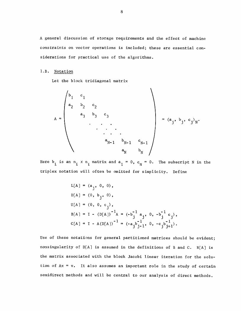
Let the block tridiagonal matrix

\a2 b2 c2

a3 b3 c3A =

= (aj, bj, cj)N.

aN- I bN- I CN- I

aN bN

Here b.1 is an n.1 × ni matrix and aI 0, cN 0. The subscript N in the

triplex notation will often be omitted for simplicity• Define

L[A] = (aj, 0, 0),

DIAl = (0, bj, 0),

U[A] = (0, 0, cj),

B[A] I (D[A])- IA (-b-I I= - = . a., 0, -b-J .] 3 cj) ,

C[A] = I- A(D[A]) i= (-a.b- 0 -c .j j_ , ,

Use of these notations for general partitioned matrices should be evident;

nonsingularity of DIAl is assumed in the definitions of B and C. B[A] is

the matrix associated with the block Jacobi linear iteration for the solu-

tion of Ax = v. It also assumes an important role in the study of certain

semidirect methods and will be central to our analysis of direct methods•

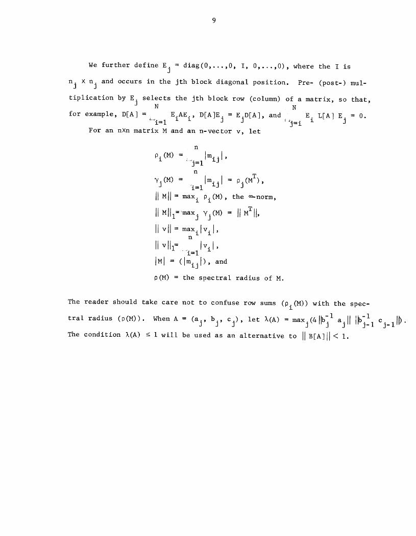
We further define E. = diag(0,...,0, I, 0,...,0), where the I isJ

n. × n. and occurs in the jth block diagonal position. Pre- (post-) mul-J J

tiplication by E. selects the jth block row (column) of a matrix, so that,J N N

for example, D[A] = E.AE D[A]Ej = E D[A], and E L[A] E = 0._i= I i i' J _]=i i j

For an n×n matrix M and an n-vector v, let

n

0i(M ) = Imij I,_j=l

n

_j(M) = Imijl - 0j(MT),_i=l

IIMII = max i 0i(M), the o_-norm,

IIMlll=_max o YO (M) = IIMTII,

IIvlJ = maxilvil,n

IIvli= l il,.....i=l

IMI = (Imijl), and

0(M) = the spectral radius of M.

The reader should take care not to confuse row sums (0i(M)) with the spec-

J -1

" = ' ' ' = _i aj j-I I "tral radius (0(M)) When A (aj bj cj) let X(A) maxj(4 I i II J_ cj_ I_

The condition X(A) _ i will be used as an alternative to IIB[A]II < I.

i0

2. SOME INITIAL REMARKS

2.A. Analytic Tools

Much of the analysis presented in later sections involves the matrix

B[A]. Why should we consider this matrix at all?

First, it is a reasonably invariant quantity which measures the diag-

onal dominance of A. That is, if E is any nonsingular block diagonal matrix

conforming with the partitioning of A, let A* =EA , so B* = B[A*] = I-D*-IA *

= I - (ED)-I(EA) = I - D-IA = B. Thus B[A] is invariant under block scal-

ings of the equations Ax = v. On the other hand, B is not invariant under

-Ia change of variables y = Ex, which induces A' = AE . We have

-iB' = B[A'] = EBE , and for general A and E only the spectral radius o(B)

is invariant. Similarly, C[A] measures the diagonal dominance of A by

columns, and is invariant under block diagonal change of variables but not

under block scaling of the equations.

Secondly, one simple class of parallel semidirect methods (Section 7)

can be created by transforming Ax = v into A*x = v*, A* = MA, v* = Mv for

some matrix M, where IiB[A*]II << IIB[A]II• This transformation typically

represents the initial stages of some direct method. An approximate solu-

tion y = D[A*]-Iv * is then computed with error x - y = B[A*]x, so I_[A*]II

measures the relative error. Thus we study the behavior of B[A] under

various matrix transformations.

Thirdly, B[A] is the matrix which determines the rate of convergence

of the block Jacobi iteration for Ax = v. This is a natural parallel itera-

tion, as are the faster semi-iterative methods based on it when A is posi-

tive definite. It is known that various matrix transformations can affect

the convergence rates of an iteration, so we study this property.

II

Finally, B[A] and C[A] arise naturally in the analysis of block elim-

ination methods to solve Ax = v. C represents multipliers used in elimina-

tion, and B represents similar quantities used in back substitution. In

order to place upper bounds on the size of these quantities we consider

the effects of elimination on JJB[A]JJ.

Since we will make frequent use of the condition JjB[A]JJ < i we now

discuss some conditions on A which will guarantee that it holds.

Lemma 2.1. Let J- Jl + J2 be order n, JJj = jJlJ + JJ2J , and suppose K

satisfies K = JlK + J2" Then jJJJJ< 1 implies Pi(K) _ pi(J) for 1 _ i _ n,

and IIKI IIJll

Proof. From JJlJ + jJ2J = JJj we have pi(Jl) + pi(J2) = pi(J) for 1 _ i _ n.

From K = JlK + J2 we have Pi(K) N Pi(Jl ) jjKJJ+ Pi(J2 )" Suppose JJKJJ _ I.

Then Pi(K) _ pi(Jl) JJKJJ+ pi(J2) JJKJJ = pi(j) JjKJJ _ JJjjJ JJKJJ,which implies

JJKJJ _ jJJjJ JJKJJ and ! _ JJJjJ, a contradiction. Thus JJKJJ < I and

Pi(K) < Pi(J I) + Pi(J2) = pi(J). QED.

We note that if pi(Jl) # 0 then we actually have Pi(K ) < pi(J ) and

if pi(Jl) = 0 then Pi(K) = pi(J2) = pi(J). It follows that if each row of

Jl contains a nonzero element then JJKJJ < JJJJJ. These conditions are rem-

iniscent of the Stein-Rosenberg Theorem (IV3], [H8]) which states that if

J is irreducible, Jl and J2 nonnegative, J2 # 0 and p(Jl ) < I then P(J) < I

implies p(K) < p(J) and P(J) = I implies o(K) = P(J)- There are also cor-

respondences to the theory of regular splittings IV3].

Lemma 2.2. Suppose J = (I - S)K + T is order n, JJj = J(l - S)KJ + JTJ,

Pi(S) _ Pi(T), I _ i _ n. Then JJJJJ< I implies Pi(K) _ pi(J), I _ i _ n,

and so H KJJ _ JJJJJ.

12

Proof. For I < i < n, Pi(T) K Pi(T) + pi((l- S)K) = 0i(J) < JJJJJ< I,

so Pi(T) < I. Now, I > pi(J) = pi((l - S)K) + Pi(T) > Pi(K) - Pi(S)JJ KJJ

+ Pi(T) > Pi(K ) + Pi(T)(I - JjKJJ ). Suppose jJKJJ = pj(K) > I. Then

I > oj(K) + pj(T)(l - pj(K)), and we have I < Oj(T), a contradiction.

Thus jJKJJ < I and Pi (J) _ Pi(K)- QED.

If S = r in Lemma 2.2 then K = SK + (J - S), JJJ = j(l - S)KJ + JSJ

= JJ - S J + iSJ, so by eemma 2.I we again conclude JJKJJ < JJJJJ.

Similar results hold for the 1-norm.

Lermna 2.3. Let J = Jl + J2' jJj = JJl j + JJ2 j' and suppose K satisfies

K = KJ I + J2" Then JJJ JJl< i implies JJKJJI _ JJJJJl"

Proof Since jT T r jjT r j + j T r T T and" = Jl + J2' J = JJl J2 j' KT = JlK + J2

JjMJJI = JjMTJJ, we have JJjTjj= jjJJJl< i, and by Lemma 2.1, JJKJJI = JJKTjj

< jjjTjj= jjJJJl" QED.

eemma 2.4. Suppose J = K(l- S) + T, JJj = JK(I- S)J + JTJ, _i(S) _ _i(r),

i _ i < n. Then JJJJJl< I implies JJKJJI _ JJJJJl"

Proof We have _i(M) Pi(MT) jT (I sT)KT + TT. = , = - , so by Lemma 2.2

jjKTJj _ jjjrjj, and the result follows. QED.

To investigate the condition JJB[A]JJ < I, we first note that if A is

strictly diagonally dominant by rows then JJB[A]JJ < I under any partition-

ing of A. Indeed, if we take J to be the point Jacobi linear iteration

matrix for A, J I diag(A)-IA = , = ,= " ' Jl D[J] J2 J- Jl then

JjJlJj< JJJJJ< i, JJj = JJlJ + jJmJ and B[A] = (I - Jl)-iJ2 , so

jJB[A]JJ < lJJJJ < I by use of Lemma 2.1.

13

Now, if we denote the partitioning of A by the vector H = (nl,n2,...,nN)

then the above remark may be generalized. Suppose _' = (ml,m2, ...,mM) rep-

resents another partitioning of A which refines H. That is, there are inte-.-1

PlgeTs I = P0 < Pl < "'" < PN = M+I such that n. = m.. If B[A] and

1 ....j=n.-- ]

B'[A] are defined by the two partitions and II B'[A][I_<IiI _hen [[ B[A]/l

< [[B'[A][ I. This is an instance of the more general rule for iterative

methods that "more implicitness means faster convergence" (cf. [H8, p. 107])

and will be useful in Section 6. Briefly, it shows that one simple way to

decrease [[B[A][[ is to use a coarser partition.

Let us consider a simple example to illustrate these ideas. Using

finite differences, the differential equation -u - u + %,i= f on [0,112 ,xx yy

% _> 0, with Dirichlet boundary conditions, gives rise to the matrix

A = (-I, M, -I), M = (-i, 4+_ 2, -i). By Lemma 2.1, [[B[A][I < [[J[A][[ =

4/(4+_h 2) < I. Actually, since B[A] is easily determined we can give the

better estimate [[B[A][[ = 2[[ M-Ill < 2/(2+_h2).

Indeed, many finite difference approximations to elliptic boundary

value problems will produce matrices A such that [IB[A][I < I [V3]; [[B[A]] I

will frequently be quite close to I. This condition need not hold for

certain finite element approximations, so a different analysis will be

needed in those cases. Varah [VI], [V2] has examples of this type of

analysis which are closely related to the original continuous problem. In

Section 9.B we consider another approach based on a change of variable.

[[B[A][] < I is a weaker condition than strict block diagonal dominance

relative to the _-norm, which for block tridiagonal matrices is the condi-

tion ([FI], [Wl]) [[bill[ ([[aj[ + [Icj[J ) < I, I < j _ N. The general

definition of block diagonal dominance allows the use of different norms,

so for completeness we should also consider theorems based on this

14

assumption. However, in order to keep the discussion reasonably concise

this will not always be done. It is sometimes stated that block diag-

onal dominance is the right assumption to use when analyzing block elimi-

nation, but we have found it more convenient and often more general to

deal with the assumption IIB[A]II < I.

Other concepts related to diagonal dominance are G- and H-matrices.

If J = I- diag(A)-IA = L + U, where L (U) is strictly lower (upper)trian-

gular, then A is strictly diagonally dominant if IIJIl< I, a G-matrix if

II(I- ILI)-IIuI II< i, and an H-matrix if p(IJl) < I. Ostrowski [02]

shows that A is an H-matrix iff there exists a nonsingular diagonal matrix

E such that AE is strictly diagonally dominant. Varga [V4] summarizes

recent results on H-matrices. Robert JR3] generalizes these definitions

to block diagonally dominant, block G- and block H-matrices using vector-

ial and matricial norms, and proves convergence of the classical iterative

methods for Ax = v. Again, for simplicity we will not be completely gen-

eral and will only consider some representative results.

2.B. Models of Parallel Computation

In order to read Sections 3-9 only a very loose conception of a vector-

oriented parallel computer is necessary. A more detailed description is

needed for the execution time comparison of methods in Section 10. This

subsection contains sufficient information for the initial part of the

text, while additional details may be found in Appendix A, [H3], [$3], and

the references given below.

Parallel computers fall into several general classes, of which we con-

sider the vector computers, namely those operating in a synchronous manner

and capable of performing efficient floating point vector operations.

15

Examples are the array processor llliac IV, with 64 parallel processing

elements [B6], [BI2]; the Cray-l, with eight 64-word vector registers [C8];

and the pipeline processors CDC STAR-100 [C2] and Texas Instruments ASC

[Wl], which can handle vectors of (essentially) arbitrary length. These

machines have become important tools for large scientific computations,

and there is much interest in algorithms able to make good use of special

machine capabilities. Details of operation vary widely, but there are suf-

ficiently many common features to make a general comparison of algorithms

possible.

An important parallel computer not being considered here is the asyn-

chronous Carnegie-Mellon University C.mmp [W4], with up to 16 minicomputer

processors. Baudet [B7] discusses the theory of asynchronous iterations

for linear and nonlinear systems of equations, plus results of tests on

C .mmp.

Instructions for our model of a vector computer consist of the usual

scalar operations and a special set of vector operations, some of which

will be described shortly. We shall consider a conceptual vector to be

simply an ordered set of storage locations, with no particular regard to

the details of storage. A machine vector is a more specialized set of

locations valid for use in a vector instruction, usually consisting of

locations in arithmetic progression. The CDC STAR restricts the progres-

sion to have increment = I, which often forces programs to perform extra

data manipulation in order to organize conceptual vectors into machine

vectors.

We denote vector operations by a parenthesized list of indices. Thus

the vector sum w = x+y is

16

wi x.l + yi' (I _ i _ N)

Nif the vectors are in R , the componentwise product would be

w.l = xi X Yi' (i _ i _ N),

and a matrix multiplication C = AB would be

N

= bkjcij _k=l aik , (I < i _ N; 1 _ j _ N).

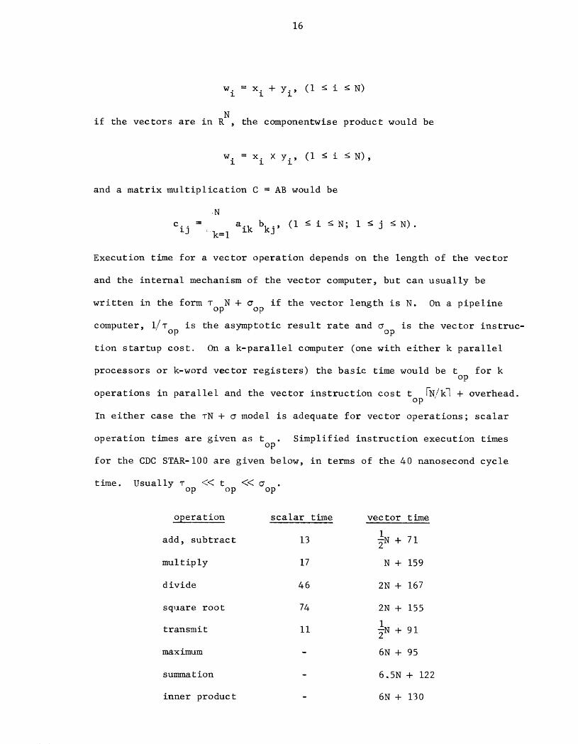
Execution time for a vector operation depends on the length of the vector

and the internal mechanism of the vector computer, but can usually be

written in the form • N + _ if the vector length is N. On a pipelineop op

computer, 1/T is the asymptotic result rate and _ is the vector instruc-op op

tion startup cost. On a k-parallel computer (one with either k parallel

processors or k-word vector registers) the basic time would be t for kop

operations in parallel and the vector instruction cost t FN/k_ + overhead.op

In either case the TN + _ model is adequate for vector operations; scalar

operation times are given as top. Simplified instruction execution times

for the CDC STAR-100 are given below, in terms of the 40 nanosecond cycle

time. Usually 'top << top << O'op.

operation scalar time vector time

I

add, subtract 13 _N + 71

multiply 17 N + 159

divide 46 2N + 167

square root 74 2N + 155

1

transmit II _N + 91

maximum - 6N + 95

summation - 6°5N + 122

inner product - 6N + 130

17

The use of long vectors is essential for effective use of a vector

computer, in order to take full advantage of increased result rates in

the vector operations. The rather large vector startup costs create a

severe penalty for operations on short vectors, and one must be careful

to design algorithms which keep startup costs to a minimum. Scalar opera-

tions can also be a source of inefficiency even when most of the code con-

sists of vector operations. Data manipulation is often an essential con-

sideration, especially when there are strong restrictions on machine vec-

tors. These issues and others are illustrated in our comparison of algo-

rithms in Section I0, which is based on information for the CDC STAR-100.

18

3. LINEAR METHODS

The simplest approach to direct solution of a block tridiagonal linear

system Ax = v is block elimination, which effectively computes an LU factor-

ization of A. We discuss the process in terms of block elimination on a

general partitioned matrix under the assumption IIB[A]II < I; the process is

shown to be linear and stable. Various properties of block elimination are

considered, such as pivoting requirements, bounds on the condition numbers

of the pivotal blocks, error propagation in the back substitution, and

special techniques for special systems. Gauss-Jordan elimination is studied

for its numerical properties, which foreshadow our analysis of the more impor-

tant odd-even elimination and reduction algorithms.

3.A. The LU Factorization

3.A.I. Block Elimination

The block tridiagonal LU factorization

A = (aj,bj,cj) N = (£j,l,0)N(0,dj,cj) N

is computed by

d =bI I

I

dj = bj - ajdi_ I Cj_l, j = 2,...,N,

_j = a.d -IJ J-l' j = 2, ...,N,

where the existence of d-Ij-I is assumed and will be demonstrated when IIB[A]II < i.

For the moment we are not concerned with the particular methods used to compute

-I

or avoid computing either _j or dj_ 1 cj_ 1•

19

Let A I = A and consider the matrix A2 which is obtained after the first

block elimination step. We have A2 = (_j,_j,Cj)N, E1 = dI = bl, _2 = 0,

92 = d2, _j = aj and _j = b° for 3 _ j < N. Let BI = B[AI] B2 = B[A2 ]-j

Note that BI and B2 differ only in the second block row; more specifically,

in the (2,1) and (2,3) positions.

Theorem 3.1. If IIB III< I then IIB211 _ IIBIII •

Proof. Let T = BIE I and let S = TB I. We have d2 = b2(l - b_la2b]Icl),--__

IIb21a2bllclll = I SII _ IIBill IIEIII IIBill = IIBII_ < I, so d21exists and

B2

is well-defined. Also, B I = (I- S)B 2 + T, IBII = I(I- S)B21 + Irl by con-

struction, and 0j(S) _ _o(T)II BIll < Pj(T). Thus eemma 2.2 applies, yielding

IIB211 < IIBIII • QED

Now, for any partitioned matrix the N stages of block elimination (no

block pivoting) can be described by the process

AI=A

for i = I,...,N-I

Ai+l = (I- L[Ai]EiD[Ai]-I)Ai= (I + L[C[Ai]]Ei)A i.

We transform Ai into Ai+ I by eliminating all the blocks of column i below the

diagonal; when A is block tridiagonal AN is the upper block triangular matrix

(0,dj,cj) N. The same effect can be had by eliminating the blocks individually

by the process

20

AI=A

for i = I,...,N-I

A (i)i+l =A. i

for j = i+l,...,N

iLA j) - (I (j-l) (j-l) I .(j-l)

i+l- - EjAi+I EiD[A ]"

i+l )Ai+l

(j-1)]Ei) (j-l)= (I + EjC[Ai+ I Ai+ I|

Ai+ I = A (N)i+l"

Each minor stage affects only block row j of the matrix. It is seen that

row j of A'J-lli+l_i_= block row j of Ai,block

block row i of A (j-l) = block row i of A ii+I

from which it follows that

j i.l EiD[A ] = EjAiEiD[Ai ] I,

so the major stages indeed generate the same sequence of matrices A.. Letl

Bi = B[Ai].

Corollary 3.1. If A is block tridiagonal and IIBIII< I then IIBi+lll < IIBill,

I _i <N-I.

The proof of Corollary 3.1 requires a bit more care than the proof of Theorem

3.1 would seem to indicate; this difficulty will be resolved in Theorem 3.2.

We should also note the trivial "error relations"

IIAi+ I - ANII < IIAi - ANII,

IIBi+ I - BNII _ IIBi - BNII.

21

These follow from the fact that, for block tridiagonal matrices,

i N

A = EjA N + E.Ai L-j=I z_j=i+I J I'

which holds regardless of the value of libIII.

Wilkinson [W3] has given a result for Gaussian elimination that is similar

to Corollary 3.1, namely that if A is strictly diagonally dominant by columns

then the same is true for all reduced matrices and IIAi+ I (reduced)III

IiA i (reduced)III. This actually applies to arbitrary matrices and not just

the block tridiagonal case. Brenner [B14] anticipated the result but in

a different context.

Our next two theorems, generalizing Corollary 3.1 and Wilkinson's observa-

tion, lead to the characterization of block elimination as a norm-non-increasing

projection method , and proves by bounding the growth factors that block

elimination is stable when lib[A]II< I. In addition, many special schemes for

block tridiagonal matrices are equivalent to block elimination on a permuted

matrix, so the result will be useful in some immediate applications.

Theorem 3.2. If libiiI< I then IIBi+ III < IIBill and IIAi+ Ill < IIAill for

I _i <N-I.

Proof. Suppose IIBill< i. We have

-I)Ai+ I = (I- L[Ai]EiD[Ai] Ai

= A i - L[Ai]E i + e[Ai]EiB i,

pj(Ai+l )_ pj(A i - L[Ai]E i) + pj(L[Ai]EiB i)

_ pj(A i - L[Ai]Ei) + 0j(L[Ai]Ei) llBill

The projections are onto spaces of matrices with zeros in appropriate positions.

22

0j(Ai - L[Ai]Ei) + 0j(L[Ai]E i)

= Pj (Ai),

SO IIAi. III_ IIA ill " Now let

Q = D[Ai]-IL[Ai]EiD[Ai]-IAi ,

so Ai+ 1 = Ai - D[Ai]Q, D[Ai+ I] -D[Ai](I- D[Q]).

Let S = D[Q]. Since

Q = (-L[Bi]Ei)(l- Bi) =-L[Bi] + L[Bi]EiB i,

S = D[L[Bi]EiBi] and IIEll < IIL[Bi]ll llEill IIBilI_ IIBill 2 < I. Thus-I

D[Ai+I] exists and Bi+ I is well-defined. It may be verified that

(I - S)Bi+ I B - S + Q. Let T = B - S + Q, J = S + T = B + Q. Sincel i I

D[Bi ] = D[Q - S] = 0, we have bIT] = 0 and IJl = ISI + ITI • Thus, by Lermna 2.I,

IIJll< I implies IIBi+ III _ IIJll • But we have, after some algebraic manipula-

tion,

J=B. +Ql

= _,k_ EkB1 i

+ EkBi(I - E + E Bi)=i+l i i '

and it follows from this expression that IIJll _ IIBill • QED

Although expressed in terms of the N-I major stages of block elimination,

it is clear that we also have, for Bi(j) --B[ iA(j)]' llBi(J)II-_ IIBi(J-1)IIand

IIA(j)iII-< IIA(J-l)iII" Moreover, as long as blocks below the diagonal are

eliminated such inequalities will hold regardless of the order of elimination.

23

We shall adopt the name "linear method" for any process which senerates

a sequence of matrices M.I such that IIB[Mi+I]II _ IIB[Mi]II, given that

IIB[M I] II< I. Thus block elimination is a linear method.

A result that is dual to Theorem 3.2 is the following.

Definition. Let_ be the reduced matrix consisting of the last N-i+l block

rows and columns of A.. (_ = A 1 = A)1

Theorem 3.3. If [[C[A][[1< 1 then [[C[_i+l][[ 1 _ [[C[_i]l[ 1, [[_i+1[] 1 _ [IQi[]1,

and IIn[Ci]Ei[[ I _ IIC[A]][l,Ci : C[Ai].

Remark. It is not true in general that [_i+lI[l < I]Cil[I if IIciIlI < i.

Proof. Let the blocks of C.l be Crop, i _ m, p _ N. Then C[_i] -(Cmp)i_n,p_N.

Let K = (Crop+ CmiCip)i+l_m,p_N

- (Cmp) i+l__ra,pNg + . (ci,i+l ... CiN).

\_Ni

Using Lemma 2.4, I[ c[_i+l][[ 1 _ [[ Ell 1 if [[ KIll < 1.

But N

yq (K) _ yq (_k= mk C_i ])i+l

+ [I " [11 Yq (El C[_i ])

\CNi

N

< yq (_ E k C_])k=i+l

+ I[C[_i][[ I _q(EiC[_i])

Ek C[_ i])5'q =i+l

24

+ _q (Ei C_ i]>

= Vq (C_ i])"

Thus IIKil I < IIc[ai]ll I < I and IIC[_i+l]ll I < IIC[_i]ll I • By construction

this implies llL[Ci]Eilll < IIC[A]II I for I _ i _ N. Now, let the blocks of A.i

be amp , I < m, p < N. Then_i+ I = (amp + Cmiaip)i+l_m,p_N , and

N

q(_+ I) _ 7q ( E ._ )%¢=i+I i l

+ II " lll_/q<Ei_2i)

N

meal)+ q(mii)_-i+l

II_i+llll< ll_illl"QED

We note that if A is symmetric then C[A] = B[A] T and Theorems 3.2 and 3.3

become nearly identical. Of course, B and C are always similar since C = DBD -I.

When A is positive definite, Cline [C3] has shown that the eigenvalues of_i

interlace those of _. . Actually the proof depends on use of the Choleskyl-i

factorization, but the reduced matrices are the same in both methods. In

consequence of Cline's result we have ll_i+ II12 < II_iI12 "

The statements of Theorems 3.2 and 3.3 depend heavily on the particular

norms that were used. It is not true in general, for example, that if

IIB[AI]III< I then IIB[Am]ll I < IIB[AI]II I or even IIB[_2]ll I _ IIB[_l]ll I" This

makes the extension to other norms quite difficult to determine.

25

3.A.2. Further Properties of Block Elimination

It is well-known that the block factorization A = LAU is given by

N

L = I- _ L[Cj]Ej=l J'

A = D[AN],N

U = I- BN = I- /'j=l Ej U[Bj].

We have therefore shown in Theorems 3.2 and 3.3 that if IIClllI < I then

IILill _ I + IICIllI < 2, IIEll _ I + Nnll CIllI, n = max.] n.,j and if IIBIll< I

then IIUil _ I + lIBl II< 2, IIUill _ 1 + Nnll BIll • (For block tridiagonal

matrices the factor N can be removed, so IILil _ 1 + nll Cllil, IIUilI _ I + rillBIll.)

Moreover, the factorization can be completed without permuting the block rows

of A. The purpose of block partial pivoting for arbitrary matrices is to

force the inequality IIL[Cj]Ejll _ i. Broyden [BI5] contains a number of

interesting results related to pivoting in Gaussian elimination. In particular

it is shown that partial pivoting has the effect of bounding the condition

number of L, though the bound and condition number can actually be quite

large in the general case. We will have some more comments on pivoting after

looking at some matrix properties that are invariant under block elimination

(cf. [BI1]).

Corollary 3.2. Block elimination preserves strict diagonal dominance.

Proof. It follows from Theorem 3.2 that Gaussian elimination preserves strict

diagonal dominance: simply partition A into IXI blocks. Now suppose we have

A i and are about to generate Ai+ I. This can be done either by one stage of

block elimination or by n. stages of Gaussian elimination, for both processesl

produce the same result when using exact arithmetic [H8, p. 130]. Thus if A.i

is strictly diagonally dominant, then so is Ai+ I. QED

26

It is shown in [B4] that Gaussian elimination maps G-matrices into

G-matrices. This can be extended in an obvious fashion to the case of block

elimination. We also have

Corollary 3.3. Block elimination maps H-matrices into H-matrices.

Proof. Recall that A is an H-matrix if and only if there exists a nonsingular

diagonal matrix E such that A' = AE is strictly diagonally dominant. Con-

sider the sequence

A{ = A' ,

A'i+l = (I- L[A_.]Ei D[A_.]'I)A_.

Clearly A I'= AIE; suppose that A'.l= AiE is strictly diagonally dominant. We

then have

A' = (I - L[A ]E E E-ID -I) °i+l i i [Ai ] A El

= (I- L[Ai]E i D[Ai]-I)Ai E

= Ai+IE,

!

so Ai+ I is an H-matrix since Ai+ I is strictly diagonally dominant by Corollary

3.2. QED

We have chosen to give this more concrete proof of Corollary 3.3 because

it allows us to estimate another norm of B[A] when A is an H-matrix. Define

IIMIIE = IIE-IMEII• Then since A' = AE implies B[A'] = E-IB[A]E it follows

that if A is an H-matrix then IIB[Ai+I]II E < IIB[Ai]IIE. Since the matrix E

will generally remain unknown this is in the nature of an existential proof.

The proof of Corollary 3.2 brings out an important interpretation of

Theorem 3.2. If block elimination is actually performed then our result

27

gives direct information about properties of the reduced matrices. If not,

and ordinary Gaussian elimination is used instead, then Theorem 3.2 pro-

vides information about the process after each n. steps. While we are notz

assured that pivoting will not be necessary, we do know that pivot selec-

tions for these n. steps will be limited to elements within the d. blocki l

for the block tridiagonal LU factorization. When A has been partitioned to

deal with mass storage hierarchies this will be important knowledge (see

Section 10.A).

One more consequence of Theorem 3.2 is

Corollary 3.4. In the block tridiagonal LU factorization, if IIB llj< I then

cond(dj) = JldjlJ IIdilll< 2 cond(bj) / (I- IIBIJI2).

Proof. Letting _j = b-la.d -I = b (I - c; ) iJ_jlJ <j j j-lCj -I' we have dj j J ,

IIBill IIBNIJ _ JlBIJ_ < i, so that IIdjJl _ Ilbjll (i + II_jIl) < 211 bjll, and

QED

It is important to have bounds on cond(dj) since systems involving d.J

must be solved during the factorization. Of course, a posteriori bounds on

IIdilll may be computed at a moderate cost. We note also that

cond(A) < max.j 2 cond(bj) / (I - lJBIll ) when IIBIII< i, and it is entirely

possible for the individual blocks b. and d. to be better-conditioned than A.J 3

The inequalities in Theorem 3.2 are the best possible under the condition

IIBIIJ < I. This is because, for example, the first block rows of B1 and B2

are identical. However, it is possible to derive stronger results by using

different assumptions about BI.

28

Theorem 3.4. [H4] For A = (aj,bj,cj), let %(A) = maxj(411 bjlajll l_]_llCj_lll),I

e. = b-ld.. If X(A) _ I then III - ejlI < (I - _)/2 and IIei II_ 2/(I + I_I-_)J J J

Some useful consequences of this theorem include better estimates for

IIBNII and a smaller upper bound on the condition numbers of the d.'S. For weJ

have BN = (0,0,-d-lc.)jJ = (0,0,-e-lb-lcj)'3J which implies that

IIBNII _ 211U[BI]II / (i + _f_). As an example, if A = (1,3,1) then Theorem

3.2 predicts only IIBNII < IIBIII= 2/3, while by Theorem 3.4 we obtain

IIBNII _ 2(I/3) / (I + ^/1-4/9) - 0.382. Also, IIdilll < IIdilbjll llbjIII=

I_iI] l_jlll_21_jlll, and l_jll <- l_j- doll+ l_jll= l_j(I " e-_ll+ l_jll _

ilboll III - ej]1+ IIb011 _ 311 bjl_2- It follows t_&t co_d(dj) = IIdilll l_jll <

3 con_(Dj). More precisely, cond(dj)_ (I + 2_(A)) cond(bj), _ = (I-^_)/(I+_).

This is further proof of the stability of the block LU factorization.

Theorem 3.4 has been used in the analysis of an iteration to compute the

block diagonal matrix (0,dj,0)N [H4]. Such methods are potentially useful

in the treatment of time-dependent problems, where good initial approximations

are available. This particular iteration is designed for use on a parallel

computer and has several remarkable properties; for details, see [H4] and

Section 8.E.

Two results on the block LU factorization for block tridiagonal matrices

were previously obtained by Varah.

Theorem 3.5. [VII If A is block diagonally dominant (IIb]111(l jll+I 011)i)

and ]]cj]] _ 0, then IId_ll] < 1]cj]r I, ]]£j]] < ]]ajl]/ ]]Cj_lll, and

IIdoll < IIboil+ IIajl"

29

In comparison to Theorem 3.2, the bound on IIdilll-' corresponds to theJ

bound IIdjlcjll < I, which follows from IIBNII < I, and the bound on [I djll

corresponds to the bound IIAN[I _ flAil- In contrast to Theorem 3.2, IIBIII< I

only allows us to conclude IId]l[l _ IIbjlll / (I - IIBIII2), and we can only

estimate II_jllin the weak form II_jCj_ll I< IIajll IId]_llCj_llI _< IIajlJ.

Varah's second result is

Theorem 3.6. [Vl] Let _. = (IIbila I 1/2j jll IIbi_l cj_lll ) , 2 _ j _ N, and sup-

pose _. # 0. Then the block LU factorization of A is numerically stableJ

(i.e., there exists a constant K(A) such that max(l I _jll ,IIdjll ) _ K(A)) if

(_j,l,_j_ I) is positive semidefinite.

We note that (_j,l,_j.l) is a symmetrization of (I[bilaj[l,l, IIbi Icjll )

and that X(A) _ 1 implies that it is positive definite. The actual bounds

on II%jll, IIdjll given by Varah IV1] for this case will not be important for

this discussion.

Since many block tridiagonal systems arise from the discretization of

differential equations, a number of results have been obtained under assump-

tions closely related to the original continuous problem. Rosser [R7] shows

that if the system Ax = v, A = (aj,bj,cj), satisfies a certain maximum

principle then A is nonsingular, the LU factorization exists (each d. is non-J

singular), BN is non-negative and IIBNII_ I. Improved bounds on BN are

obtained when A is defined by the nine-point difference approximation to

Poisson's equation. In particular there is the remarkable observation that

the spectral condition number of d. is less than 17/3. Such results dependJ

strongly on the particular matrix under consideration. For examples of

related work, see [BI8], [CI], [D2].

30

3.A.3. Back Substitution

So far we have only considered the elimination phase of the solution of

Ax = v. For block tridiagonal matrices A = (aj,bj,cj) N this consists of

the process

=b fl=Vldl I'

dj = bj - a.dl I i fJ-j j-lCj -I' fj = vj - ajd I-I I'

j = 2,...,N.

The back substitution phase consists of the process

-I

= d fN'XN N

= d-Ixj J (fj- cjxj+l), j = N-I,...,I.

In matrix terms these are the processes

AI = A, f(1) = v,

= Ci]Ei)Ai,Ai+ I (I + L[ i = I,...,N-I,

f(i+l)=(l + L[Ci]Ei)f (i) i = i N-I

g = x(N) = D[AN I-If(N),

x (i) x (i+l) i = N-I, I= g + EiBN , ..., ,

(I)X = X

An alternate form of back substitution is

x (N) = D[AN]-If (N) '

X (i)(I + BNE i+l)x (i+l)

= , i = N-I,...,I,

(1)X -" X

31

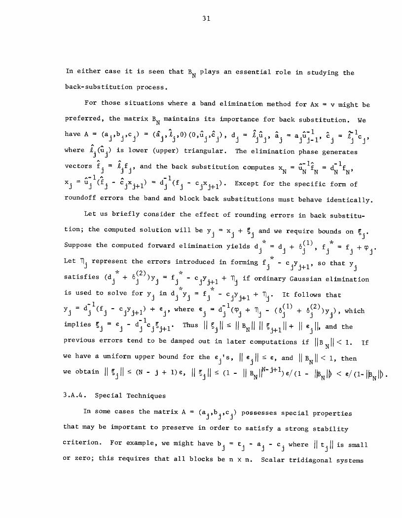
In either case it is seen that BN plays an essential role in studying the

back-substitution process.

For those situations where a band elimination method for Ax = v might be

preferred, the matrix BN maintains its importance for back substitution. We

^ _j ^ ^j) ^^ ^ ^-I _-Ihave A = (aj,bj,c.) = (a 0) (0 j, ' j J j' j ] j-l' j ] ]3 j, , ,u c d = _.u a = a.u c = _. c.,

where _.j(uj^ ) is lower (upper) triangular. The elimination phase generates

. ^ ^_I_- NIfNvectors f = %.f , and the back substitution computes xN UN fN d] ] J = = ,^--1 #% ^

x. = u. (f - c.x ) = d'l _] ] j J j+l j (fj cjxj+l). Except for the specific form of

roundoff errors the band and block back substitutions must behave identically.

Let us briefly consider the effect of rounding errors in back substitu-

tion; the computed solution will be yj = xj + _j and we require bounds on _j.* (I) *

Suppose the computed forward elimination yields d. = d. + 6.] _I .I ' f" = f +q0j] J "

2--

Let _j represent the errors introduced in forming fj - cjyj+l, so that yj* (2) *

satisfies (d.j + 6.j )yj = fj - cjyj+l + _j if ordinary Gaussian elimination

is used to solve for yj in dj yj = f.j - cjyj+ 1 + _j. It follows that

yj = d-l(fjj - cjyj+l) + Cj' where cj = d-l(_jj + _j - (8!1)J + 6(2))yj)j, which

implies _j = ej - d-lcj j_j+l" Thus II_jll _ IIBNII II_j+lll + IIcjll, and the

previous errors tend to be damped out in later computations if I;BNII< I. If

we have a uniform upper bound for the ¢.'sj, IIejll _ ¢, and IIBNII < I, then

we obtain II_jll _ (N - j + i)¢, II_jll < (I - IIBNI_-J+I)_/(I - I_NI_ < e/(l-l_Nl _.

3.A.4. Special Techniques

In some cases the matrix A = (aj,bj,cj) possesses special properties

that may be important to preserve in order to satisfy a strong stability

criterion. For example, we might have b.] = t.]- a.j - c.] where IIt011 is small

or zero; this requires that all blocks be n × n. Scalar tridiagonal systems

32

with this property arise from the discretization of second order ODE boundary

value problems. Babuska [BI-3] has discussed a combined LU - UL factoriza-

tion for such a matrix which allows a very effective backward error analysis

to the ODE and a stable numerical solution of a difficult singular pertur-

bation problem posed by Dorr [D3]. (See [H7] for a symbolic approach to

this problem.)

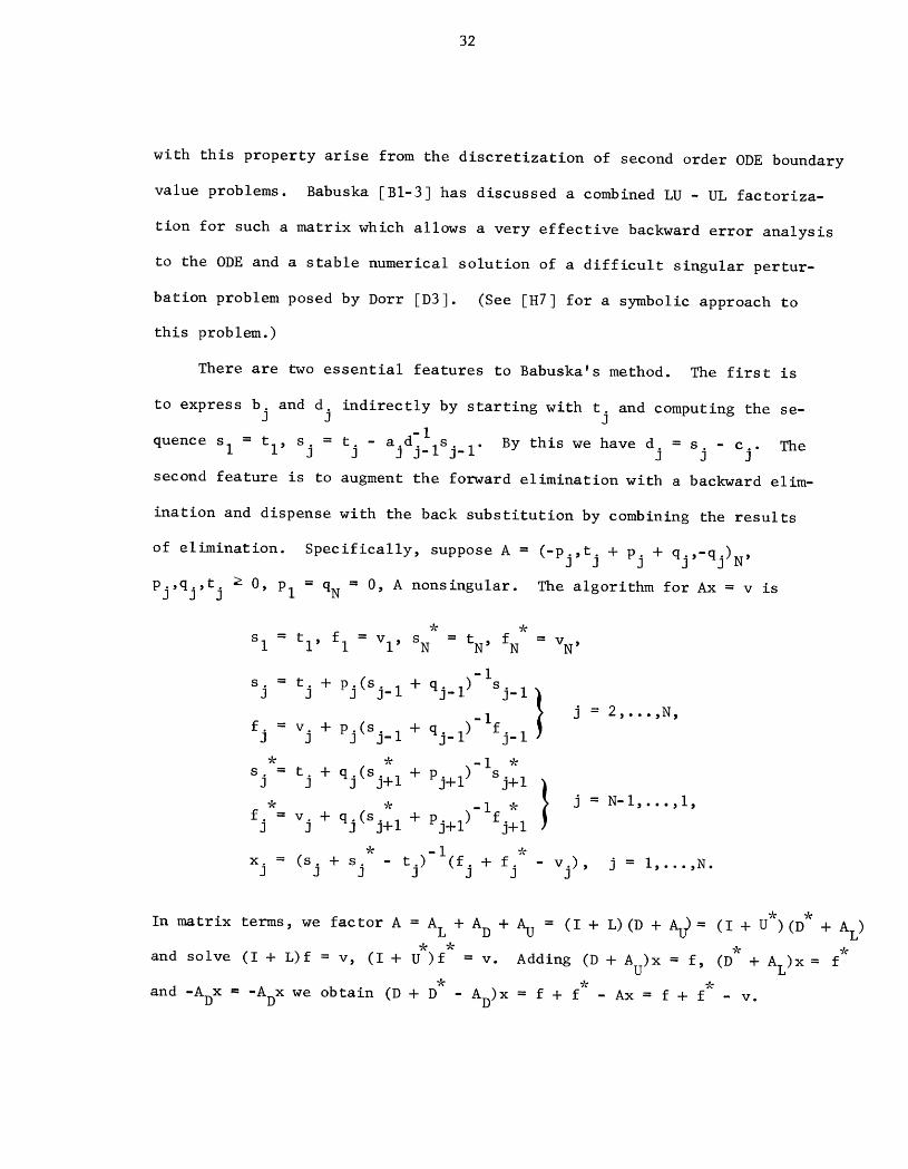
There are two essential features to Babuska's method. The first is

to express b. and d° indirectly by starting with t. and computing the se-J J J

= = - ajd_ lls j ....quence sI tl, sj tj _ _I By this we have dj = sj - cj. The

second feature is to augment the forward elimination with a backward elim-

ination and dispense with the back substitution by combining the results

of elimination. Specifically, suppose A = (-pj,tj + pj + qj'-qj)N'

0 Pl = qN = 0, A nonsingular. The algorithm for Ax = v ispj,qj,tj ,

= fNSl = tl' fl Vl' SN = tN' = VN'

-i

sj = tj + pj(sj_ I + qj_l ) Sj_l }fj = vj + pj(sj_ I + qj-I )-Ifj-I J = 2,...,N,

* * -I *

sj = tj + qj(sj+ I + Pj+l ) sj+ I

* (s * -I * I

J N-I,...,1,

fj = vj + qj j+l + Pj+I ) fj+l

* -I *

x°j = (sj + s.j - tj) (fj + fj - v.),j j = I,...,N.

In matrix terms, we factor A = AL + AD + AU = (I + L)(D + A_ = (I + U )(D + AL)

and solve (I + L)f = v, (I + U )f = v. Adding (D + Au)X = f, (D + AL)X = f

and -ADX ---ADX we obtain (D + D - AD)X_ = f + f - Ax = f + f - v.

33

Babuska's algorithm has some unusual round-off properties (cf. [M3])

and underflow is a problem though correctable by scaling. It handles small

row sums by taking account of dependent error distributions in the data,

and thus fits into Kahan's notion that "conserving confluence curbs ill-

condition" [KI].

To see how the method fits in with our results, we note that, for n = I,

d-lls _ t.. Thus the rowsince pj,qj,tj _ 0 we have sI _ 0, sj = tj + pj j_ j-I ]

sums can only increase during the factorization. On the other hand, they

-I

will not increase much since sj = tj + pj(sj_ I + qj_l ) sj. I < tj + Pj"

These are analogues of the results in Theorem 3.2.

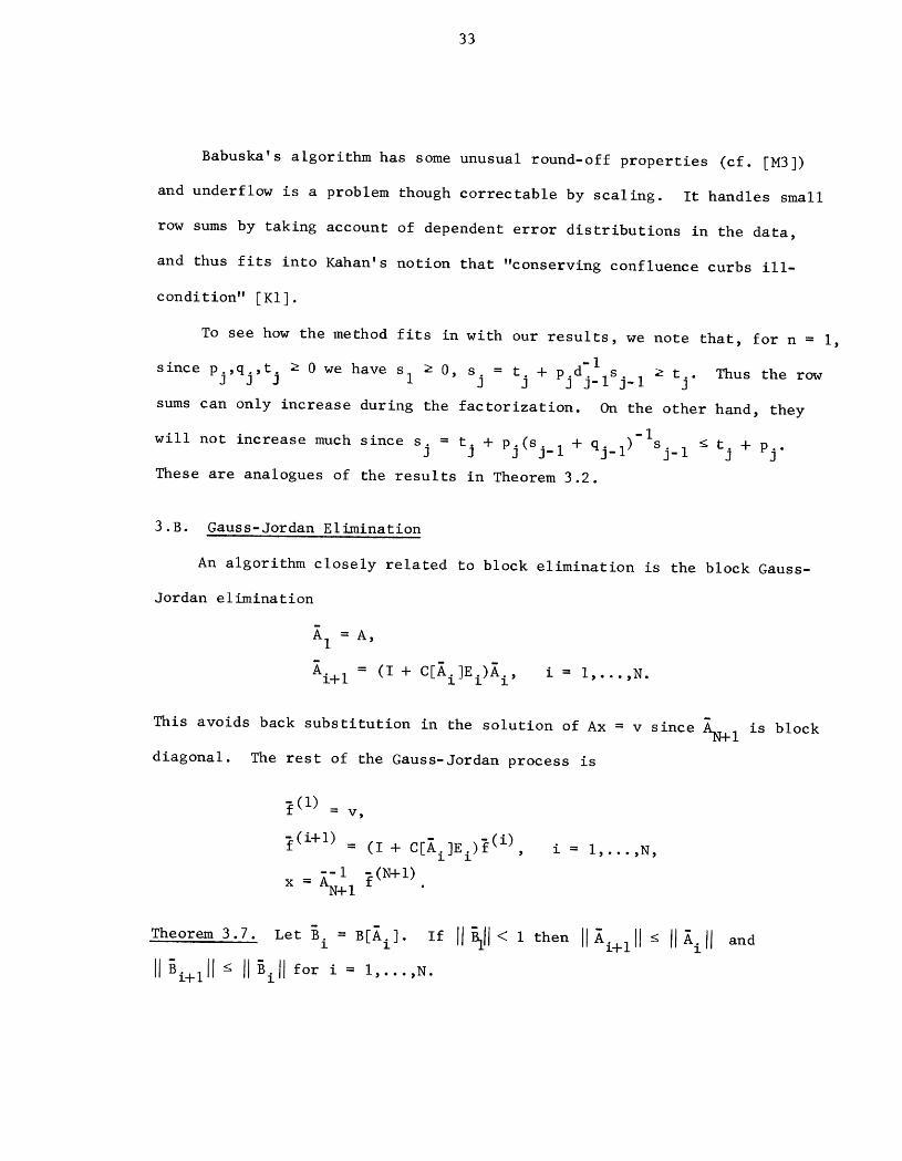
3.B. Gauss-Jordan Elimination

An algorithm closely related to block elimination is the block Gauss-

Jordan elimination

21 = A,

Ai+l = (I + C[Ai]Ei)Ai, i = I,...,N.

This avoids back substitution in the solution of Ax = v since _+I is block

diagonal. The rest of the Gauss-Jordan process is

2(1)= v,

_(i+l) = (I + C[Ai]Ei)f (i) i = I, ,N

--1 _(N+I)x = AN+ I

Theorem 3.7. Let Bi = B[Ai]" If II_II < I then IIAi+lll < IIAill and

IIBi+lll _ IIBill for i = I,...,N.

34

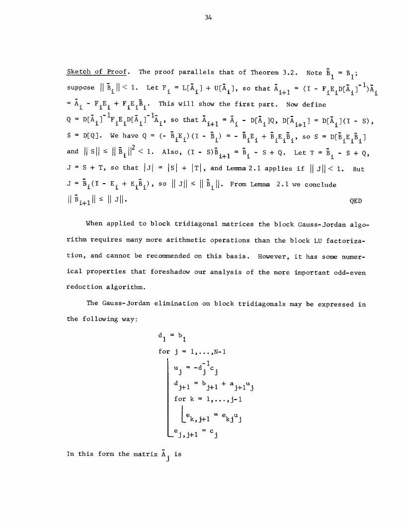
Sketch of Proof. The proof parallels that of Theorem 3.2. Note B = BI 1;

- _ - -l)i.suppose IIBill < I. Let Fi = L[Ai] + U[Ai] , so that Ai+ I - (I - FiEiD[Ai] l

= A. - F.E. + F.E.B.. This will show the first part Now definei i i i i i

Q = D[Ai]-IFimiD[Ai]-iEi , so that Ai+ I = Ei - D[Ai]Q, D[Ai+l] = D[Ai]( I _ S),

S = D[Q]. We have Q = (- BiEi )(I- Bi ) = - BiEi + BoE Bi' so S = D[BiE- ]i i i i

IISII _ IIBill2 < I. Also, (I - S)Bi+ I = B. - S + Q. Let T = B - S + Qand

i i '

J = S + T, so that IJl = ISl + ITI, and eemma2.1 applies if IIJll< I. But

J = Bi(l - E.z + E.B.)zz ' so I]Jl] < IIBill" From eemma 2.I we conclude

IIBi+lll _ ]IJll" QED

When applied to block tridiagonal matrices the block Gauss-Jordan algo-

rithm requires many more arithmetic operations than the block LU factoriza-

tion, and cannot be recommended on this basis. However, it has some numer-

ical properties that foreshadow our analysis of the more important odd-even

reduction algorithm.

The Gauss-Jordan elimination on block tridiagonals may be expressed in

the following way:

dI = bI

fo_ j = I,...,N-I

-Iu. =-d. c.J ] ]

dj+ I = bj+ I + aj+lU j

for k = l,...,j-I

Lek,j+ I = ekju j

ej,j+ I = c.]

In this form the matrix A. is]

35

elj

d2 e2j

d3 e3j

dj-I ej-l,j

0 d. c.J J

aj+l "'. bj+l aN...Cj+l DN''"//

-- m , _ • • • m -.with AN+ I - diag(d I d2 ,dN) = D[AN] , BN+ I 0.

-I

We observe that, for i < j <j +k < N, -dj ej,j+ k = ujuj+l...Uj+k_l,

k Thus we are able to refine Theorem 3 7which is the (j,j + k) block of BN.

by giving closer bounds on the first i-i block rows of B..l

Corollary 3.5• If JIBiij < I and (point) row _ is contained in block row

j with I _ j < i-l, then

P_(Bi ) < II-d-le i-jllj ji II< IIBN •

If (point) row £ is contained in block row j with i < j < N, then

0z(Bi ) = P_(B i) < IIBill •

This is our first result on the convergence to zero of portions of a

matrix during the reduction to a block diagonal matrix• It also provides

a rather different situation from Gauss-Jordan elimination with partial

pivoting applied to an arbitrary matrix [PI]. In that case the multipliers

above the main diagonal can be quite large, while we have seen for block

36

tridiagonal matrices with II B1 II < 1 that the multipliers actually decrease

in size.

3.C. Parallel Computation

We close this section with some remarks on the applications and inher-

ent parallelism of the methods; see also [H3]. When a small number of

parallel processors are available the block and band LU factorizations

are natural approaches. This is because the solution (or reduction to tri-

angular form) of the block system d.u. = -c. is naturally expressed inJ J J

terms of vector operations on rows of the augmented matrix (dj l-cj), and

these vector operations can be executed efficiently in parallel. However,

we often cannot make efficient use of a pipeline processor since the vec-

tor lengths might not be long enough to overcome the vector startup costs.

Our comparison of algorithms for a pipeline processor (Section 10.C) will

therefore consider the LU factorization executed in scalar mode. We also

note that the final stage of Babuska's LU-UL factorization is the solution

of a block diagonal system, which is entirely parallel.

On the other hand, the storage problems created by fill-in with these

methods when the blocks are originally sparse are well-known. For large

systems derived from elliptic equations this is often enough to disqualify

general elimination methods as competitive algorithms. The block elimina-

tion methods will be useful when the block sizes are small enough so that

they can be represented directly as full matrices, or when a stable implicit

representation can be used instead.

37

4. QUADRAT IC METHODS

In Section 3 we have outlined some properties of the block LU factor-

ization and block Gauss-Jordan elimination. The properties are character-

ized by the generation of a sequence of matrices M. such thatl

IIB[Mi+ I]II _ IIBIN i]ll" From this inequality we adopted the name "linear

methods". Now we consider some quadratic methods, which are characterized

by the inequality IIB[Mi+ l]II < IIB[M i]211"

There are two basic quadratic methods, odd-even elimination and odd-

even reduction. The latter usually goes under the name cyclic reduction,

and can be regarded as a compact version of the former. We will show that

odd-even elimination is a variation of the quadratic Newton iteration for

-iA , while odd-even reduction is a special case of the more general cyclic

reduction technique of Hageman and Varga [HI] and is equivalent to block

elimination on a permuted system. Both methods are ideally suited for use

on a parallel computer, as many of the quantities involved may be computed

independently of the others [H3]. Semidirect methods based on the quadratic

properties are discussed in Section 7.

4.A. Odd-Even Elimination

We first consider odd-even elimination. Pick three consecutive block

equations from the system Ax = v, A = (aj,bj,cj):

ak-IXk -2 + bk-lXk -I + Ck-lXk = Vk-I

(4.1) akXk_ I + bkX k + CkXk+ I = vk

ak+iXk + bk+iXk+ I + Ck+iXk+ 2 = Vk+ I

we multiply equation k-I by -akbkl kIIf

-i' equation k+l by -Ckb I' and add, the

result is

38

(-akbil Iak- i)Xk- 2

+ (bk - akbillCk_ I - Ckbkllak+l)X k

(4.2)

+ (-Ckbkl iCk+ I)Xk+ 2

= (vk - akbkllVk_ I - CkbkllVk+l)"

For k = I or N there are only two equations involved, and the necessary

modifications should be obvious. The name odd-even comes from the fact

that if k is even then the new equation has eliminated the odd unknowns

and left the even ones. This is not the only possible row operation to

achieve this effect, but others differ only by scaling and possible use of

a matrix commutativity condition.

By collecting the new equations into the block pentadiagonal system

(2) it is seen that the row eliminations have preserved the factH2x = v

that the matrix has only three non-zero diagonals, but they now are farther

apart. A similar set of operations may again be applied, combining equa-

tions k-2, k and k+2 of H2 to produce a new equation involving the unknowns

(3)Xk_ 4, xk and Xk+ 4. These new equations form the system H3x = v .

The transformations from one system to the next may be succinctly ex-

pressed in the following way. Let HI = A, v (I) = v, m = Flog2 N_, and define

Hi+ I = (I + C[Hi])Hi,

(i.l) i = 1,2 ,m.v = (I + C[Hi])v(i), ,...

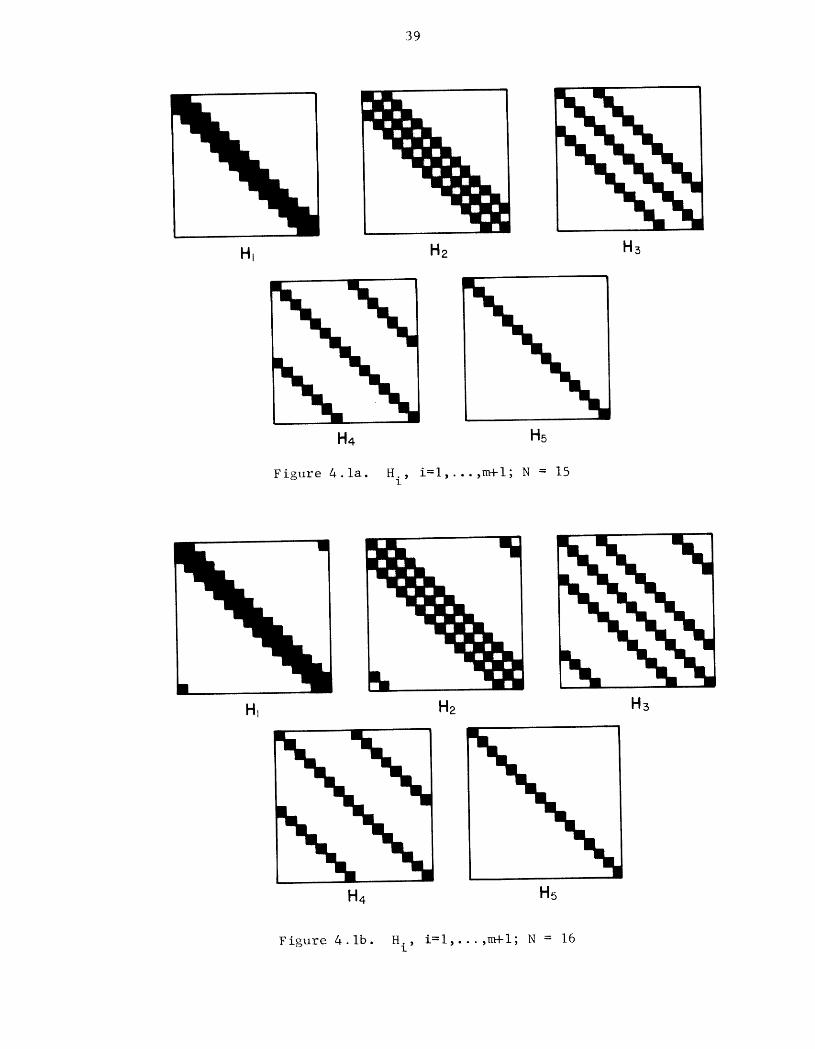
Block diagrams of the H sequence for N = 15 are shown in Figure 4. la. The

distance between the three non-zero diagonals doubles at each stage until

the block diagonal matrix Hm+ I is obtained; the solution x is then obtained

-I v(m+l)bY x = Mm+ I

39

Hi H2 H3

H4 H5

Figure 4.1a. H., i=l,...,m+l; N = 151

Figure 4.lb. H., i=l,...,m+l; N = 16l

40

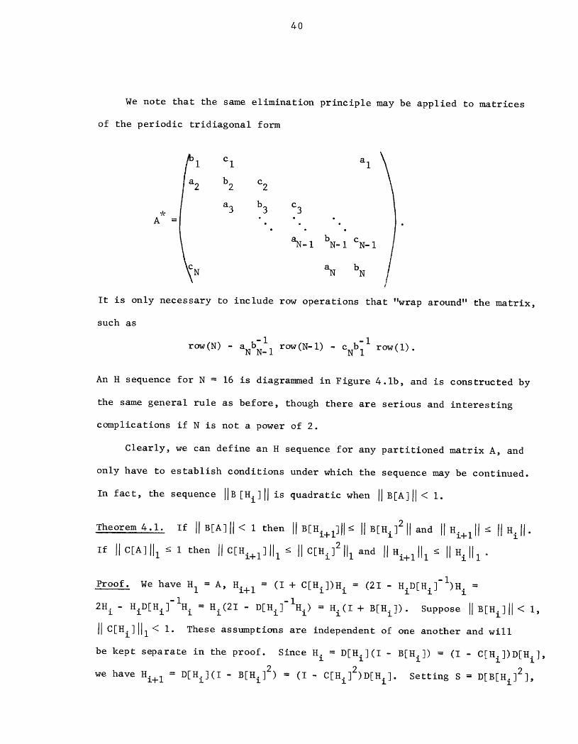
We note that the same elimination principle may be applied to n_trices

of the periodic tridiagonal form

1 Cl al

a2 b2 c2

a3 b3 c3

A ._. • • • • • • •

aN_ I bN_ I CN_ I

N aN bN

It is only necessary to include row operations that "wrap around" the matrix,

such as

row(N) - aNDNII_ row(N-l) -CNb:l row(l)•

An H sequence for N = 16 is diagrammed in Figure 4.1b, and is constructed by

the same general rule as before, though there are serious and interesting

complications if N is not a power of 2.

Clearly, we can define an H sequence for any partitioned matrix A, and

only have to establish conditions under which the sequence may be continued.

In fact, the sequence lIB[Hi]l[ is quadratic when [JB[A][ I< I.

Theorem 4•1. If lJB[A]II < I then IIB[Hi+I]II< JlB[Hi]211 and JlHi+llJ :< IIHilJ.

< ]2If IIC[A]III i then IIC[Hi+I]II I < IIC[H i III and IIHi+lllI _ IIHillI '

-1)Proof• We have H I = A, Hi+ I = (I + C[Hi])H i = (21 - HiD[Hi] H =I

2H i HiD[Hi]-IH = iHi ) .- i Hi(21 - D[Hi]- = Hi(l + B[Hi]) Suppose IIB[Hi]ll < I,

IIC[Hi]ll I < I. These assumptions are independent of one another and will

be kept separate in the proof• Since Hi = D[Hi](I - B[Hi] ) = (I - C[Hi])D[Hi] ,

= _ = ]2we have Hi+ I D[Hi](l- B[Hi ]2) = (I C[Hi]2)D[Hi ]. Setting S D[B[H i ],

41

]2T = D[C[H i ], we obtain D[Hi+I] = D[Hi](I- S) = (I- T)D[Hi]. Since

, _ IIC[Hi]211 < I, and D[Hi] is invertibleIISll < IIB[Hi]21; < 1 IITilI I

"iHi+it follows that D[Hi+I] is invertible. We have B[Hi+I] = I - D[Hi.I] i=

I (I - S)-ID ID[Hi 2- [Hi]- ](I- B[Hi]2), so B[Hi] = (I- S)B[Hi+I] + IS;

similarly C[Hi ]2 = C[Hi+I](I - T) + T. Now, S is block diagonal and the

block diagonal part of B[Hi+l] is null, so IB[Hi]21 = I(I- S)B[Hi+I] I + ISI.

Lemma 2.2 now applies, and we conclude IIB[Hi+ I]II < IIB[Hi ]211" Lemma 2.42

implies that IIC[Hi+I]II I < IIC[H i] III" To show IIHi+ill _ IIHill if-I

IIB[Hi]ll< I, write Hi+ I = D[Hi](I- D[H i] (D[Hi] - Hi)B[Hi]) = D[H i]N

\,

+ (H - D[Hi])B[Hi]. We then have for I < % _ n.,i ' _j=l J

0k(Hi+ 1) _ 0%(D[Hi]) + P_(H i - D[Hi])II B[Hi]II

p%(D[Hi]) + 0k(Hi - D[Hi])

= 0_(Hi) •

To show llHi+l}ll _ {lIIi{{lif {{C[Hi]{II < I, write Hi+ I = <I- C[Hi]<D[H i] - Hi) X

D[Hi]-I)D[Hi ] = D[Hi] + C[Hi](H i - D[Hi] ). We have

_(Hi+ I) _ 7%(D[H i]) + IIC[H i]ll 7_(H i " D[H i])

<__/%(D[Hi]) + _/%(Hi - D[H i])

= v£(H i) • QED

For a block tridiagonal matrix A we have B[Hm+I] = 0 since Hm+ I is

block diagonal; thus the process stops at this point. The proof of Theorem

4.1 implicitly uses the convexity-like formulae

Hi+ I = Hi B[H i] + D[Hi](I- B[Hi])

= C[Hi]Hi+ (I- C[Hi])D[Hi].

42

As with Theorems 3.2 and 3.3, it is not difficult to find counterexamples

to show that Theorem 4. I does not hold for arbitrary matrix norms. In

]2particular, it is not true that IIB[A]II2 < I implies IIgCH2]ll2 _ IIg[H I 112

or even that IIBIN 2]II2 < I.

The conclusions of Theorem 4.1 are that the matrix elements, considered

as a whole rather than individually, do not increase in size, and that the

off-diagonal blocks decrease in size relative to the diagonal blocks if

I{B[A]{I < I. The rate of decrease is quadratic, though if IIB[A]II is.very

close to I the actual decreases may be quite small initially. The relative

measure quantifies the diagonal dominance of Hi, and shows that the diagonal

elements will always be relatively larger than the off-diagonals. One con-

clusion that is not reached is that they will be large on an absolute scale.

Indeed, consider the matrix A = (-1,2+¢,-1), for which the non-zero diagonals

of H. areI

2

el = ¢' ek+l = 4ek + ek .

l-iFor small ¢ the off-diagonal elements will be about 2 and the main diagonal

2-i .elements about 2 in magnitude. While not a serious decrease in size,

periodic rescaling of the main diagonal to I would perhaps be desirable.

As already hinted in the above remarks, a more refined estimate of

IIB[Hi+l]II may be made when dealing with tridiagonal matrices with constant

diagonals [$2]. Let A = (a,b,a), so that

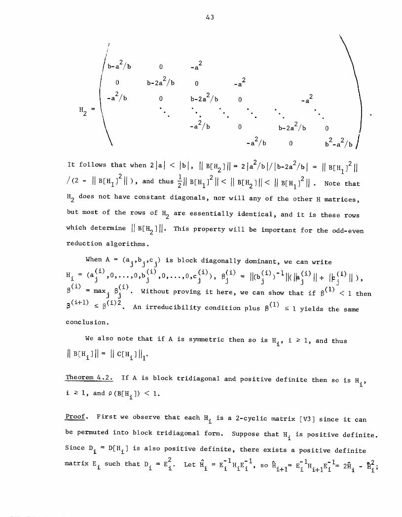
43

I/

/ 2b-a2/b 0 -a

0 b-2a2/b 0 -a2

-a2/b 0 b-2a2/b 0 -a2• • • • • •

H2 = .. ". ". ". ". ". •

, -a2/b 0 b-2a2/b 02 b2 /-a /b 0 -a2/b

It follows that when 21al < Ibl, IIB[H2]II = 21a2/bl/Ib-2a2/bl = IIB[H I]211

]2 i 2/(2- IIB[H I II), and thus _IIB[HI] II< IIB[H2]II< IIB[HI]211 . Note that

H2 does not have constant diagonals, nor will any of the other H matrices,

but most of the rows of H2 are essentially identical, and it is these rows

which determine IIB[H2]II" This property will be important for the odd-even

reduction algorithms•

When A = (aj,bj,cj) is block diagonally dominant, we can write

= a 0 0 0 0Hi ( j , , , , j , , , , j _j = II(b ) If( II+ l-j ,

_(i) = max. _!i) . Without proving it here, we can show that if _(I) < I thenJ J

_(i+l) _ _(i)2. An irreducibility condition plus 8(1) _ I yields the same

conc lus ion.

We also note that if A is symmetric then so is Hi, i e I, and thus

Jl B[Hi]II = IJ C[Hi]IJI"

Theorem 4.2. If A is block tridiagonal and positive definite then so is H.,l

i _ i, and p_ __(B[Hi]) < I.

Proof• First we observe that each H. is a 2-cyclic matrix IV3] since it canl

be permuted into block tridiagonal form. Suppose that Hi is positive definite.

Since Di = D[Hi ] is also positive definite, there exists a positive definite

2 E-IH-I so E IHi+IE-il= _ - "H.2matrix Ei such that Di = E_.l Let i = l iEi ' Hi+l = _ 2-i i

44

Hi and Hi+l are positive definite iff H.l and Hi+ I are positive definite.

Since H'l is a positive definite 2-cyclic matrix, we know from Corollary 2

of Theorem 3.6 and Corollary I of Theorem 4.3 of IV3] that P(Bi)< I B = I -' i i"

Since B I D- IH E" i^• = - = B.E it follows that p (Bi) < I also. Let X be1 l i 1 I i'

^ ^

an eigenvalue of H..l Then -I < I-X < I since P(Bi) < I, and so we have

0 < X < 2 and 0 < 2X- X2 < I. But 2X- X2 is an eigenvalue of H = 2H.-H2_i+l l i

which is therefore positive definite. QED

Any quadratic convergence result such as Theorem 4.1 calls to mind the

Newton iteration. If _<Y,Z) = Y(2I- ZY) = (2I- YZ)Y, y(0) is any matrix

with III - ZY (0) II < i for some norm II" II_, and y(i+l) = _(y(i),z) ' then

y(i) converges to Z-I if it exists and (I - ZY (i+l)) = (I- zY(i))2[H8].

It may be observed that Hi+ I = _(Hi,D[Hi ]-I) , so while the H sequence is not

a Newton sequence there is a close relation between the two. Nor is it

entirely unexpected that Newton's method should appear, cf. Yun [YI] and

Kung [K2] for other occurrences of Newton's method in algebraic computations.

Kung and Traub [K3] give a powerful unification of such techniques.

The Newton iteration y(i+l) = 9_(y(i),z) is effective because, in a

certain sense, it takes aim on the matrix Z-I and always proceeds towards it.

We have seen that odd-even elimination applied to a block tridiagonal matrix

eventually yields a block diagonal matrix. The general iteration

Hi+ I = 91(Hi,D[Hi ]-I) incorporates this idea by aiming the it-h step towards

the block diagonal matrix D[Hi]. Changing the goal of the iteration at each

step might be thought to destroy quadratic convergence, but we have seen

that it still holds in the sequence IIB[H i]ll"

45

4.B. Variants of Odd-Even Elimination

There are a number of variations of odd-even elimination, mostly dis-

cussed originally in terms of the odd-even reduction. For constant block

diagonals A = (a,b,a) with ab = ba, Hockney [H5] multiplies equation k-I

by -a, equation k by b, equation k+l by -a, and adds to obtain

(-a2)xk_2 + (b2 _ 2a2)xk + (-a2)xk+2 = (bvk - avk_ I - aVk.l).

This formulation is prone to numerical instability when applied to the dis-

crete form of the Poisson equation, and a stabilization has been given by

Buneman (see [B20] and the discussion below).

With Hockney's use of Fourier analysis the block tridiagonal system

Ax _ v is transformed into a collection of tridiagonal systems of the form

(-I,X,-I)(sj) = (tj), where X e 2 and often X >> 2. It was Hockney's obser-

vation that the reduction, which generates a sequence of Toeplitz tridiagonal

matrices (-I,X (i),-l), could be stopped when I/_ (i) fell below the machine pre-

cision. Then the tridiagonal system was essentially diagonal and could be

solved as such without damage to the solution of the Poisson equation.

Stone [$2], in recommending a variation of cyclic reduction for the

parallel solution of general tridiagonal systems, proved quadratic conver-

gence of the ratios I/X (i) and thus of the B matrices for the constant

diagonal case. Jordan [Jl], independently of our own work [H2], also extend-

ed Stone's result to general tridiagonals and the odd-even elimination algo-

rithm. The results given here apply to general block systems, and are not

restricted solely to the block tridiagonal case, though this will be the

major application.

46

We now show that quadratic convergence results hold for other formu-

lations of the odd-even elimination; we will see later how these results

carry over to odd-even reduction. In order to subsume several algorithms

into one, consider the sequences HI = A, v(I) = v,

Hi+l = Fi(2D[Hi] - Hi)GiHi'

v-(i+l) = Fi(2D[_i ] _ Hi)Giv(i )

where F., G. are nonsingular block diagonal matrices. The sequence H. cor-i l i

-i

responds to the choices F = I, G = D[Hi] .i i

In the Hockney-Buneman algorithm for Poisson's equation with Dirichlet

boundary conditions on a rectangle we have

T bT=bA = (a,b,a), ab = ba, a = a,

F. diag (b(i_ Hi ]-Ii = ,Gi= D[ ,

b (I) = b, b (i+l) = b(i)2 - 2a (i)2,

(i) (i+l) _ (i)2a = a, a - -a .

Sweet [SIll also uses these choices to develop an odd-even reduction algo-

rithm. We again note that the H. matrices lose the constant diagonal prop-i

erty for i m 2, but symmetry is preserved. Each block of H. may be repre-l

sented as a bivariate rational function of a and b; the scaling by F° en-i

i

sures that the blocks of block rows j2 of Hi+ I are actually polynomials in

a and b. In fact, the diagonal blocks of these rows will be b (i+l)_-and the

(i+l)non-zero off-diagonal blocks will be a

Swarztrauber [$6] describes a Buneman-style algorithm for separable

elliptic equations on a rectangle. This leads to A = (aj,bj,cj) where the

blocks are all n × n, and aj = _jln, bj = T + _jln, cj = Vjln. In this

case the blocks con_nute with each other and may be expressed as polynomials

47

in the tridiagonal matrix T. Swarztrauber's odd-even elimination essenti-

ally uses F = diag(LCM (i) b(i) * (i)i (bj_2i_ I, j+2i_l )) , bj = In for j _ 0 or

j _ N + I, G i = D[Hi ]-I. Stone [$2] considers a similar algorithm for tri-

(i) (i) = D[Hi]-idiagonal matrices (n = I) but with F i = diag(bj_2i_l bj+2i_l) , G i

Note that symmetry is not preserved.

In all three cases it may be shown by induction that Hi+l = Fi"" "FIHi+I

and v (i+l) = F .... F v (i+l)l I . These expressions signal the instability of

the basic method when Fj # I [B20]. However, in Section 2.A we showed that

the B matrices are invariant under premultiplication by block diagonal

matrices, so that B[Hi] = B[Hi].

The Buneman modifications for stability represent the v (i) sequence by

sequences p(i) q(i) with v (i) = D[Hi]p(i) + q(i) Defining D = D[i_i], • •

1

Qi = _'l - Hi' Si - D[QiGiQi] and assuming DiGiQ i = QiGiDi , we have

P(1) = 0, q(1) = v(1) = v,

P (i+l) (i) I (i) (i)= P + D-l (Qi p + q )

- (i+l)q(i+l) = Fi(_iGiq(i) + SiP ).

Theorem 4.3. Let PI = I, Pi = B[Hi-I]'''B[HI]' i a 2. Then p(i) = (I- Pi)x,(i)

m -- --

q = (DiPi Qi )x

Remark. Although not expressed in this form, Buzbee et al. [B20] prove spe-

cial cases of these formulae for the odd-even reduction applied to Poisson's

equation.

Proof. To begin the induction, p(1) = 0 = (I - Pl)X, q(1) = v = HI x

-- -- --" -- ' m °= (DIP I - Ql)X. Suppose p(i) (I P.)x q(i) _ (_._ _ _ )x. Then

LCM = least common multiple of the matrices considered as polynomials in T.

48

m m

p(i+l) = (I - Pl)X + D-I(Qi(ll - Pi )x + (DiPi - Qi )x)

= (I - Pi + D-.I- i-i Qi - Di QiPi + _-I_._ii i - _.l_i)x

= (I - B[H i]Pi)X

I

= (I - Pi+l )x

and q(i+l) = v(i+l) _ -Di+lp(i.l)

= i+lx - 5i+l(I->i+l)X1 I

= (Di+l" Qi+l - Di+l + Di+IPi+l )x1 i i

= (Di+iPi+l - Qi+l )x. QED

i-I

We note that when Gi = D[Hi ]-I and 8 = IIB[A]II < i then I_ill = 132 -i < I

and Pk(DiPi- Qi ) _ 0k(Di)II Pill+ pk(Qi ) < Pk(Di ) + 0k(Q i) = Pk(Hi ), so

IIDiPi - Qill _ IIHill • It also follows that IIx - p(i)II _ IIPill IIxll and

IIq(i) + _ixl I _ IIDiPill IIxll • Thus p(i) will be an approximation to x;

Buzbee [BI7 ] has taken advantage of this fact in a semidirect method for

Poisson's equation.

4.C. Odd-Even Reduction

4.C.I. The Basic Algorithm

The groundwork for the odd-even reduction algorithms has now been laid.

Returning to the original derivation of odd-even elimination in (4.1) and

(4.2), suppose we collect the even-numbered equations of (4.2) into a

linear system A(2)x (2) = w (2) where

-I -i -I -I

A(2) = (-a2jb2j-la2j-l'b2j" a2jb2j-lC2j -I - c2jb2j+la2j+l'-C2jb2j+ic2j+l)N2'

x (2) = (x2j)N2'

49

w(2) -i -I = (2)

= (v2j - a2jb2j_IV2j_l- c2jb2j+iv2j+l)N2 (v2j)N 2

N2 = _N/2j.

This is the reduction step, and it is clearly a reduction since A (2) is half

(2)the size of A (I) = A Once A(2)x (2) w has been solved for x (2)• = we can

compute the remaining components of x (I) = x by the back substitution

i

x2j_l = b2j_l(V2j_l - a2j_ix2j_2 - c2j_ix2j), j = I,..., FN/2_.

Since A (2)is block tridiagonal we can apply this procedure recursively

to obtain a sequence of systems A (i)x(i) = w(i), where A(1) = A, w(1) = v,

x (i) = (xj2i_l) N , NI = N, Ni+ I = _Ni/2j We write A (i) a(i) b(i) (i)i " = ( J , j ,cj )Ni,

x (i) Flog2J" = xj2i_ I. The reduction stops with A(m)x (m) = w(m) , m = N+I_

(note the change in notation) since A (m) consists of a single block. At

this point the back substitution begins, culminating in x (I) = x.

Before proceeding, we note that if N = 2m-I then N. = 2m+l-i - i. Thel

odd-even reduction algorithms have usually been restricted to this particular

choice of N, but in the general case this is not necessary• However, for

A = (a,b,a) N there are a number of important simplifications that can be

made if N = 2m-I [B20]. Typically these involve the special scalings men-

tioned earlier, which effectively avoid the inversion of the diagonal blocks

during the reduction•

It is also not necessary to continue the reduction recursively if

(k)A(k)x (k) = w can be solved more efficiently by some other method. This

leads to various polyalgorithms and the semidirect methods of Section 7.

By the way in which A (i) has been constructed, it is clear that it

consists of blocks taken from H i. For example, in Figure 4.1a, A (4) is

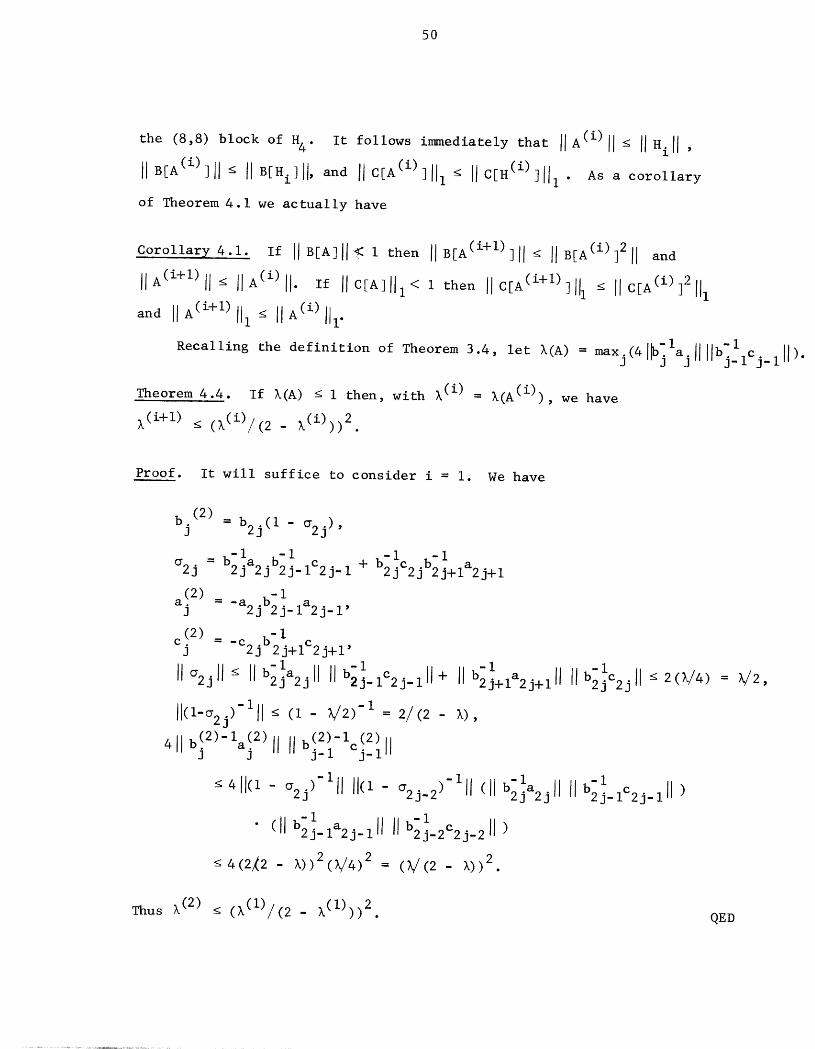
50

the (8,8) block of H4. It follows immediately that IIA(i) II< IIHill ,

IIB[A(i)]II _ IIB[Hi]II, and IIC[A(i)]III _ IIC[H(i)]II I • As a corollary

of Theorem 4. I we actually have

Corollary 4.1. If IIB[A]II _< I then IIB[A(i+I)]II _ IIB[A(i)]211 and

llA(i+l) l]_ ]IA(i) ll. If IIC[A]III < I then IIC[A(i+l)]Ill _ IIC[A(i) ]2111

and IIA(i+l)II 1 _ IIA(i) IIl-

Recalling the definition of Theorem 3.4, let %(A) --maxj(41_] lajllllb-llcj_lj II)

Theorem 4.4. If X(A) _ I then, with %(i) = %(A(i)), we have

%(i+I) _ (%(i)/(2 - _(i)))2.

Proof. It will suffice to consider i = I. We have

b (2)= b2 (i- _2j )J j '

_2j = b21 -i b21 -Ija2jb2j- IC2j-I + jc2jb2j+la2j+l

a(2) -Ij = -a2jb2j_ la2j_ I,

(2) -ljc o = -c2jb 2J +IC2j+l '

IIo2jll _ IIb21 IIIIb21jamj j_Icmj_lll + IIb21 -ij+la2j+lll llbmjC2jll < 2(_/4) = _2,

ll(l-_2j)-lll< (I- _2) -I = 2/(2- _),

411 b(2)-la(2)jj IIIIb(m)-l-(mj_lcj-_ II

< 411(1 - _2j)-lll II(I - _2j_2)-III (IIb21 ija2jll IIb2j_ic2j_lll )

I

• (IIb2j_la2j iii IIb21- j-2Cmj-2 II)

4(2_2 - _))2(_4)2 = (_(2 - _))2.

Thus _(2) _ (_(I)/(2 - _(I) 2)) • QED

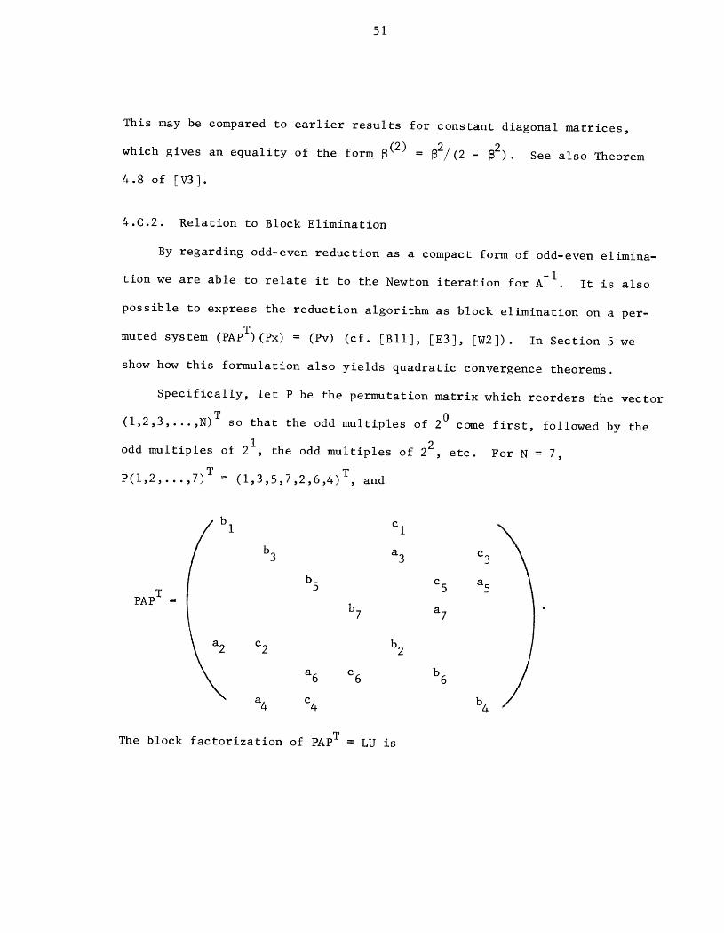
51

This may be compared to earlier results for constant diagonal matrices,

which gives an equality of the form _(2) = _2/(2 _ _2). See also Theorem

4.8 of IV3].

4.C.2. Relation to Block Elimination

By regarding odd-even reduction as a compact form of odd-even elimina-

-Ition we are able to relate it to the Newton iteration for A . It is also

possible to express the reduction algorithm as block elimination on a per-

muted system (PAPT) (Px) = (Pv) (cf. [BII], [E3], [W2]). In Section 5 we

show how this formulation also yields quadratic convergence theorems.

Specifically, let P be the permutation matrix which reorders the vector

T 0(1,2,3,...,N) so that the odd multiples of 2 come first, followed by the

odd multiples of 21 22, the odd multiples of , etc. For N = 7,

T TP(1,2,...,7) = (1,3,5,7,2,6,4) , and

b I cI

b3 a3 c3

b5 c5 a5

pAp T = b7 a7 •

c2 b2

a6 c6 b6

a4 c4 b4

The block factorization of PAP T = LU is

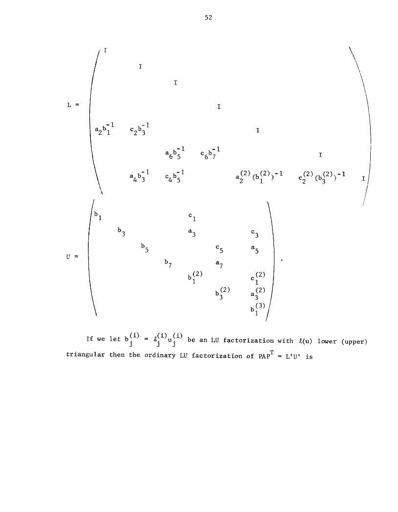
52

iI i 1L = I

a2bll c2b31 I

a6b51 c6b71 I

. a4b31 c4b51 a2(2)(b(2))-ll c2(2)(bJ2)'-l, I/

b3 a3 c3

b5 c5 a5U =

b7 a7 "

(2) _2)b I c

bJ2) aJ2)/

(i) _ _!i)u(i ) be an LU factorization with _(u) lower (upper)If we let bj - J J

triangular then the ordinary LU factorization of PAP T = L'U' is

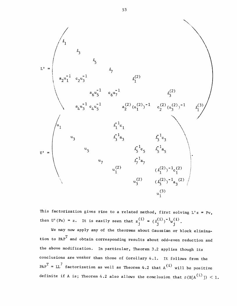
53

_3

L' = _7

1 a2ull c2u31 (2)i 4\ -1 -1 _(2)

a6u5 c6u7 _3

" - - c - %__\\ a4u31 c4u51 a_2)(u_2)) I _2)(u_2)) I

_llCl

u3 _la 3 _Ic 3

u5 _Ic 5 _la 5U' = i.

u7 _la 7

(2) 2,_2) -1 (2)Ul ( ) _1

...._ (2) _2) - I (2) _% u3 (_ ) a3 i

(3)u I

This factorization gives rise to a related method, first solving L'z = Pv,

Z (i) = (" -1_ (i)then U' (Px) = z. It is easily seen that (%7i)) w.

J 3 3

We may now apply any of the theorems about Gaussian or block elimina-

tion to PAP T and obtain corresponding results about odd-even reduction and

the above modification. In particular, Theorem 3.2 applies though its

conclusions are weaker than those of Corollary 4.1. It follows from the

pAp T = LL7 factorization as well as Theorem 4.2 that A (i) will be positive

definite if A is; Theorem 4.2 also allows the conclusion that p(B[A (i)]) < I.

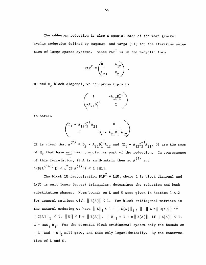
54

The odd-even reduction is also a special case of the more general

cyclic reduction defined by Hageman and Varga [HI] for the iterative solu-

tion of large sparse systems. Since PAPT is in the 2-cyclic form

_i AI2_

pAp T =

21 D2/

D1 and D2 block diagonal, we can premultiply by

2 IDI I

to obtain

1 - A12D2 A21

- 1A0 D2 - A21D 1

1D11A 12 - - 1A2It is clear that A (2) = D2 - A2 and (D 1 A12D 2 1' 0) are the rows

of tt2 that have not: been computed as part of the reduction. In consequence

of this formulation, if A is an M-matrix then so A (i) and

0(B[A (i+l)]) < p2(B[A(i)]) < 1 [H1].

The block LU factorization PAP T = L&U, where A is block diagonal and

L(U) is unit lower (upper) triangular, determines the reduction and back

substitution phases. Norm bounds on L and U were given in Section 3.A.2

for general matrices with IIB[A]I] < 1. For block tridiagonal matrices in

the natural ordering we have IILIIl < I + IIC[A]III, IILII <nll C[A]III if

IIC[A]III < i, IIUII _ I + IIB[A]II, IIUIII _ I + nll B[A]I I if IIB[A]II < I,

n = max. n.. For the permuted block tridiagonal system only the bounds onJ J

IILII and IIUIII will grow, and then only logarithmically. By the construc-

tion of L and U,

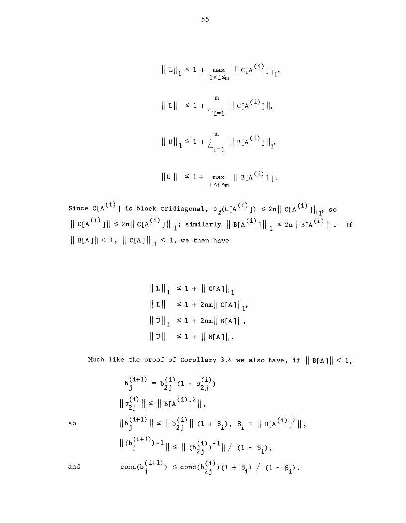
55

IILII__ _+ max IIC[A(_)lll_,1_i-<m

m

II_11_ _+ IIC[A(i)311,_i=l

m

I+ Li I IIBEA(i)]III'IIullI =

IluII _ _. max IIBEA(i)]II"l_i-_n

Since C[A (i)] is block tridiagonal, P%(C[A(i)]) _ 2nll C[A(i)]III' so

IIC[A(i) ]II_ 2nll C[A(i)]II I; similarly IIB[A(i) ]II i _ 2nll B[A(i)II • If

IIB[A]II < I, IIC[A]II I < I, we then have

IILII1 _ 1+ IIc[AllllII LII _ 1 + 2_ll CEA]II1,

IIulI1 _ 1+ 2nmllBEA]II,IIUII _ 1+ IIN[AIlI.

Mu=h_ikethep=oofof Co=o_=y3.4we_o h_ve,if IIB[AILI< _,

b(i+l) = b_ i) _)J j (i- )

;I_ i) II_ IIB[A(i)]211j

. h(i) = ,(i+l) II_ II-2j II(I + _i), _i IIB[A(i) ]211

II(b(i+l)) -I ib(i) IJ II_ II )-II/(_-_i)'2j

and cond(b!i+l)) _ c°nd(b_ ))(I + 8i) / (1- _i).3

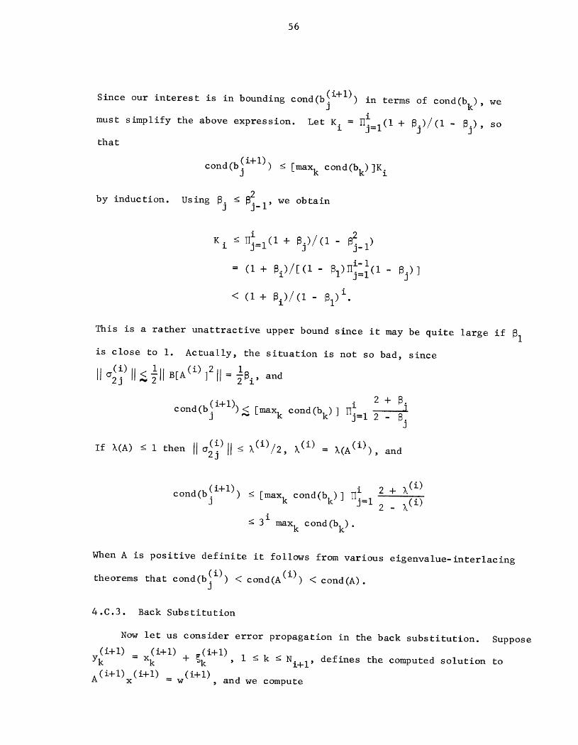
56

(i+l)) in terms of cond(b k) weSince our interest is in bounding cond(bj

must simplify the above expression• Let K. = iI _j=l (I + _j)/(l- 8j), so

that

cond(b_ i+l)) _ [max k cond(b k) ]K i

by induction Using Sj _ _2j.• I' we obtain

i 2

K i < _j=l(l + _j)/(l - _j_l )

i-i

= (I + _i)/[(l- _l)IIj=l(l- 8j)]

< (I + _i)/(l - _i)i.

This is a rather unattractive upper bound since it may be quite large: if 61

is close to I. Actually, the situation is not so bad, since

I (i) ]2 1II°2j-(i> II<_ _II B[A II= _8i' and

2+8cond (b (i+l)) J

j _< [max k cond(b k) ] Hi• j=l 2 - 8j

_i) %( (i) i)If X(A) < i then II_ j II_ i)/2, k = %(A ( ), and

i 2 +_ %_i_l_

c°nd(b_ i+l)) _ [maxk c°nd(bk)] _j=l 2 _(i)

i

< 3 max k cond(bk) .

When A is positive definite it follows from various eigenvalue-interlacing

theorems that cond(b_ i)) < cond(A (i)) < cond(A).

4.C.3. Back Substitution

Now let us consider error propagation in the back substitution. Suppose

(i+l) (i+l) (i+l)Yk = Xk + _k , I _ k _ hi+l, defines the computed solution to

A(i+l) (i+l) w (i+l) and we computeX -_

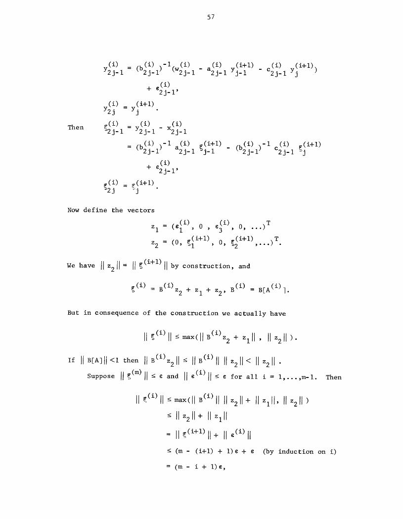
57

(i) = (b_i) l)-l(w_i) a(i) _ (i+l) c(i) (i+l))Y2j-I j- j-I- 2j-I Yj-! - 2j-I Yj

¢(i)+ 2j-l'

(i) = y_i+l)Y2j

Then F(i) = y_i) _ x_i)_2j-i j-i j-I

= (b_i) l)'I a(i) F(i+l) (b_!l)-I c (i) _(i+l)j- 2j-I =j-I " 2j-I j

+ ¢ j-l'

_i) (i+l)j = _j •

Now define the vectors

0E 1 ' , _ _ -..

= _(i+l) 0 _2(i+l),- ..)

T

z2 (0, hI , , • •

We have IIz211= II_(i+l)II by construction, and

_(i) = B(i) z2 + Zl + z2 ' B(i) = B[A(i)].

But in consequence of the construction we actually have

II_(i) ll< max(ll B(i)z2 + Zlll ' IIz211 )"

If 1[ B[A][[ <1 then [I B(i) z2[[ _ [[ B(i) II [[ z21[ < II z2[[ •

Suppose [[ _(m)I[ _ ¢ and ][ e (i) [[ < ¢ for all i = 1,...,m-1. Then

II_(i)II _ma_(I[B(i)[[IIz2[I+ IIz_II,IIz211)

[Iz2 II+ IIzIll

--II_(i+_)II+ II_(i)II

(m- (i+l) + I)¢ + ¢ (by induction on i)

= (m- i + I)¢,

58

and II_(I)II, the error in the computed solution of Ax = v, is bounded by

me, m = [log2 N + I]. This is certainly a satisfactory growth rate for

error propagation in the back substitution. In fact, it is a somewhat

pessimistic upper bound, and we can more practically expect that errors in

the solution of A(i+l)x(i+l) = w (i+l) will be damped out quickly owing to

the quadratic decreases in IIB(i)II •

4.C.4. Storage Requirements

On the matter of fill-in and storage requirements, we note that block

elimination in the natural ordering of A, as discussed in Section 3.A, re-

quires no additional block storage since there is no block fill-in. However,

it has already been seen that odd-even reduction does generate fill-in. The

(2) (m)amount of fill-in is the number of off-diagonal blocks of A ,...,A ,

m

which is 2(N i - i) < 2N. Since the matrix A requires 3N- 2 storage-Ji-2

blocks, this is not an excessive increase. Of course, we have not considered

the internal structure of the blocks, as this is highly dependent on the

specific system, nor have we considered temporary storage for intermediate

compu tat ions.

We do note, however, that if the factorization need not be saved, then

some economies may be achieved. For example, in the transition from A (I)

(2)to A (2) , the first equation of A(2)x (2) = w is generated from the first

three equations of A(1)x (I) = w (I). The first and third of these must be

saved for the back substitution, but there is no reason to save the second

once A(2)x (2) = w (2) is formed. Thus the first equation of A(2)x (2) = w (2)

(1)may overwrite the second equation of A(1)x (I) = w . Similar considera-

tions hold throughout the reduction, but some modifications are needed on

the CDC STAR-100 due to its restrictions on vector addressing (see Section 10.B).

59

The special scalings of odd-even reduction for systems derived from

separable elliptic PDE's allow implicit representation of the blocks of

A (i) as polynomials or rational functions of a single matrix variable.

Since the blocks of A are quite sparse this is necessary in order to limit

intermediate storage to a small multiple of the original storage. Unfor-

tunately, there does not seem to be a similar procedure that can be applied

to nonseparable PDE's. The only recourse is to store the blocks as dense

matrices, and on current computing systems this will limit them to small

sizes.

4.C.5. Special Techniques

Now suppose that A = (-pj,tj + pj + qj, -qj), pj,qj,tj _ 0, pl= qN= 0;

we would like to apply Babuska's tricks for the LU factorization (Section

3.A.4) to the factorization induced by odd-even reduction. This only par-

(2) t(2) + _(2) + q(2) (2))tially succeeds. First, we can represent A (2) = (-pj , J pj J ,_qj

where

(2) b21Pj = P2j j-i P2j-I'

t(2) -I b21 t2j = t2j + P2j b2j-I t2j-i + q2j j+l j+l'

(2) b21qj = q2j j+l q2j+l'

bk = tk + Pk + qk"

Note that t2j < t(2) _ b2 On the other hand the technique of avoidingj j"

the back substitution by combining the LU and UL factorizations of PAPT

pApT J- , ,will not work. Let A' = = (I + L)(D + U) = (I + U")(D + L ), (I + L)f= Pv,

(D + U)(Px) = f, (I + U )f = Pv, (D + L )(Px) = f , so that

* 2" *

(D + D - D[A' ])(Px) = f + f - (L + D[A' ] + U)(Px).

60

The only way to have A' = L + D[A' ] + U is if no fill-in occurs in

_,¢

either factorization, in which case L = L[A' ], U = U[A]. In particL,lar

fill-in occurs in odd-even reduction, so the method does not work in its

entirety. However, it will still be advantageous to do the reductions by

developing the t(i) sequences. (See [Sl] for some examples.)

Schr_der and Trottenberg [SI] also consider a method of "total reduc-

tion" for matrices drawn from PDE's and finite difference approximations

on a rectangular grid. Numerical stability and further developments are

discussed in [Sla]. The total reduction is similar to odd-even reduction

(which is derived in [Sl] by a "partial reduction"), but just different

enough to prevent the application of our techniques. Part of the problem

seems to be that total reduction is more closely related to the PDE than

to the matrix, though the algorithm is expressible in matrix form. Various

convergence results are undoubtedly obtainable, but we have not yet deter-

mined the proper setting for their analysis.

4.D. Parallel Computation

Finally, the utility of the odd-even methods for parallel or pipeline

computation has been demonstrated in several studies [H3]. Stone [$2],

Lambiotte and Voigt [L2], and Madsen and Rodrigue [MI] discuss odd-even

2'¢

reduction for tridiagonal systems, and conclude that it is the best method

to use when N is large (> 256). Jordan [Jl] considers odd-even elimination,

which is shown in [MI] to be most useful for middle ranges of N (64 <i N < 256)

on a particular pipeline computer, the CDC STAR-100. For small values of

N the sequential LU factorization is best, owing to the effect of lower order

terms engendered by the pipeline mechanism.

The basic method given here is a block analogue of the method examined in [L2].

61

The inherent parallelism of the odd-even methods is in formation of

the equations of A(i+l)x(i+l) - (i+l) (i.l)- w or Hi+ix = v and in the back

substitution for odd-even reduction. It is readily seen from (4.2) that

(1)H2 and v (2) may be computed from HI and v by

compute LU factors of bk, (I < k < N)

solve bk[a k _k Vk] = [ak Ck Vk]' (i _ k _ N)

bk(2) - bk - ak_k_ I - CkSk+ I, (I < k < N)

Vk(2) +-v k - akV_k_l- CkVk+ I, (I _ k < N)

ak(2) +- -akak-l' (3 _ k _ N)

k(2) ^c _- -CkCk+ I, (I < k _ N - 2)

(Special end conditions are handled by storing zeros strategically or by

(2)shortening vector lengths slightly. A (2) and w are computed by only gen-

erating new equations for even k; the back substitution is then rather

straightforward once x (2) is computed.

The algorithm for odd-even reduction, N = 2m-l, all blocks n X n,

N. = 2m+l-i - I, is as follows: for i = l,...,m-Il

LU factors of b(i) (0 _ k < N i)compute

2k+l' i+

(i) ^ ^ ra(i) c(i) w(i)solve b2k+l[a2k+l C2k+l W2k+l ] = L 2k+l 2k+l 2k+l ], (0 < k < Ni+l)

k - a C2k_l- c a2k+l, (I _ k < Ni+l)

^ i

wk(i+l) = W2(k)- a_k)W2k_l C_k)W2k+l , (I £ k < Ni+l)

ak(i+l) = _a2(k) ^ (2 < k <a2k- I' Ni.l)

ck(i+l) =-C_k) C2k+l' (I _ k < Ni+l - I)

62

solve b_m) x_m) = w_ m)

for i = m-1,...,l

solve h (i) (i) _ . (i) _(i) _ (i+l) - c(i) x(i+l)-2k+l X2k+l - (W2k+l - a2k+l Xk 2k+l k+l ), (0 < k < Ni+ I)

The ith reduction and corresponding back substitution uses

2 3 .(12 n + O(n2))Ni+l 12n3 arithmetic operations, and the total operation

count for the algorithm is (123N--- 12m)n 3 + O(n2N + n3). This may be com-

2 3

pared to 4_Nn + O(n2N + n3) operations for solution of Ax = v by the LU

factor iza tion.

,For a crude estimate of execution time on a pipeline computer, we

take TN + _, T << _, as the execution time for operations on vectors of

length N, and t, T << t << _, as the execution time for scalar operations

[H3]. The total execution time for odd-even reduction would then be

roughly (122n 3 + o(nm))(_N + om) + O(n3t) versus (42 n3N + o(nmN + nB))t

for the LU factorization done completely in scalar mode. A qualitative

comparison shows results similar to the more precise analysis given to

tridiagonal systems: for a fixed value of n, odd-even reduction will be-

come increasingly more effective than the LU factorization as N increases.

Odd-even elimination should maintain its utility for moderate values of N;

the factor TN + om is replaced by (_N + _)m, but data manipulation is often

much simpler than in odd-even reduction. The actual crossover points be-

tween algorithms are implementation dependent and will be considered to

a limited extent in Section 10.C.

A critical observation on the execution time of odd-even reduction is

that roughly 50_ of the total time is spent in the first reduction from

.2.I,

A more detailed timing analysis is in Section 10.C and Appendix B.

63

A (I) = A to A (2). Special efforts to optimize the algorithm by solving

the reduced systems differently must take this fact into account. Further-

more, in timing each reduction it is seen that roughly 60_ of the high-

order term n3N comes from the matrix multiplications used to compute A(i+l)

and 30_o from solving the 2n+l linear systems for a2k+l' etc. Relatively

little effort is used to factor the b! i)'s or to make back substitutionsJ

having saved the factorizations.

The use of a synchronous parallel computer creates some constraints

on implementation which are not so important on a sequential computer.

The first restriction in the interests of efficiency is that the blocks of

A should all be the same size. This allows simultaneous matrix operations

(factoring, etc.) to be programmed without resorting to numerous special

cases due to varying block sizes. In addition, pivoting causes ineffi-

ciencies when the pivot selections differ between the diagonal blocks.

As with the LU factorization, the assumption [[B[A][[ < I only guarantees

that no block pivoting is needed. If A is strictly diagonally dominant

or positive definite, then no pivoting within the blocks will be required.

Thirdly, the choice of data structures to represent the matrices and

vectors must conform to the machine's requirements for the parallel or

vector operations. This is an important problem on the CDC Star owing

to its limitations on vector addressing and allocation ILl]. When A is

restricted to having small blocks this is not as serious as it would be

otherwise. In the case of the llliac IV, the problem of data communica-

tion between processing elements must also be considered.

64

4. E. Summary

We now summarize the results of this section. The odd-even elimina-

tion and reduction algorithms may be safely applied to the solution of

certain block tridiagonal linear systems, and in some cases various impor-

tant quantities involved in the solution decrease quadratically to zero.

The quadratic convergence may be explained by expressing the methods as

Newton-like iterations to compute a block diagonal matrix. Variations of

the basic methods, which have important applications to PDE's, also dis-

play quadratic convergence. Parallel computation is a natural format for

these methods, although practicalities place some restrictions on the

type of system that can be solved efficiently.

65

5. UN IFICAT ION : ITERAT ION AND F ILL- IN

Having presented several linear and quadratic methods, we now treat

them in a unified manner as particular instances of a general nonstationary

iteration. We are also lead to an interpretation of quadratic convergence

in terms of matrix fill-in, and conclude that the odd-even methods are the

only instances of the general iteration which display quadratic convergence.

These results apply to arbitrary matrices satisfying I B[A]II < I and not

only to the block tridiagonal case.

Let us first collect the formulae for the block LU factorization,

block Gauss-Jordan, and odd-even elimination.

"I)A iLU: Ai+ I = (I- L[Ai]EiD[Ai] , A I = A.

GJ: Ai+l = (I - (e[Ai] + g[Ai])EiD[Ai]-l)Ai , AI = A.

OE: Hi+ I = (I - (L[Hi] + U[Hi])D[Hi]-l)Hi , H I = A.

Now consider the function F(X,Y,Z) = (21- XY)Z, and observe that

-i

Ai+ I = F(D[Ai] + L[Ai]E i, D[A i] , Ai)

Ai+l = F(D[Ai] + (L[Ai] + U[Ai])Ei' D[Ai ]-I' Ai )

-I

Hi+ I = F(Hi, D[H i] , H i)

Thus it is necessary to analyze sequences based on repeated applications

of F.

For fixed nonsingular Y we can define the residual matrices

r(M) = I- MY, s(M) = I - YM, so F(X,Y,Z) = (I + r(X))Z and

r(F(X,Y,Z)) = r(Z) - r(X) + r(X)r(Z),

s(F(X,Y,Z)) = s(Z) - s(X) + s(X)s(Z).

66

By taking X = Z and assuming that IIr(Z I) II< i or IIs(Z I) II< I, the sta-

-I

tionary iteration Zi+ I = F(Zi,Y,Zi) converges quadratically to Y . This

is, of course, the Newton iteration.

The related operator G(X,Y,Z) = Z + X(I - YZ) - Z + Xs(Z) has pre-

viously been studied as a means of solving linear systems [H8]. When

ZI = X, Zi+l = G(X'Y'Zi)' Bauer [B8] observes that r(Zi+l) = r(X)r(Zi) ,

s(Zi+l) = s(X)s(Zi)' Zi = (I- r(X) i)Y-I = Y-I(I- s(X) i), Zi+k = G(Zk'Y'Zi)'

and in particular Z2i = G(Zi'Y'Zi)" This last formula also leads to the

- (_i)2Newton iteration, for G(Z,Y,Z) = F(Z,Y,Z), s(Z2i ) = s

In this section we study the nonstationary iteration ZI = A,

-I

Zi+l = F(Xi'Yi'Zi)' where Y.I = D[Zi] and Xi consists of blocks taken

from Z., including the diagonal. The selection of blocks for IX. is al-l i

lowed to change from step to step, but we shall assume that the selection

sequence is predetermined and will not be altered adaptively. (The cost

of such an adaptive procedure, even on a highly parallel computer, would

be prohibitive. )

For the solution of a linear system Ax = v we take (Zl,V I) = (A,v),

(Zi+l, vi+ 1) = (21 - XiYi)(Zi,vi), with the sequence ending in or approach-* * * *-i*

ing (Z ,v ), where Z is block diagonal. Then x = Z v . One necessary

- = I + r (Xi) be nonsingular,condition for consistency is that 21 XiY i i

which holds if and only if P(ri(Xi)) < i. Since ri(X i) and si(Xi) = I - Y.X.i i

are similar we could also assume P(si(Xi)) < I. Using earlier notation,

ri(Xi) = C[Xi] , si(Xi) = B[Xi] ; the notation has been changed to provide

greater generality. In the context of an iteration converging to a block

diagonal matrix, the condition IIB[A]II < I (implying IISl(X I) II_ l_l(Z I) II< I)

states that A is sufficiently close to a particular block diagonal matrix,

namely D[A].

67

We first generalize earlier results on linear methods (llsi(Zi)II< I =

IISi+l(Zi+ I) II< IIsi(Z i) II) and then determine conditions under which we

obtain a quadratic method (IIsi(Z i) II< I = IISi+l(Zi+ I) II< IIsi(Z i) 112).

Theorem 5.1 In the sequence Zi+ I = F(Xi,Yi,Zi), suppose that

[(p,p) ]I _ p _ N] c T. c {(p,q)]I _ p,q < N} = Ul-I

Xi = _.EpZ.E , Y = D[Zi] ,i q ii

si(M)__ = I- Y.M.I

Then IIsI(ZI> II< I implies

IISi+l(Zi+ I) II_ IIsi(Zi+l> iI< IIsi(Zi> II•

Proof. Suppose IIsi(Z i) II< I. Define Q by Zi+ I = Zi " D[Zi ]Q' so

Q = -YiZi + Y1"XiY'Zli =-si(Xi) + si(Xi)si(Zi). Since D[si(Xi) ] = 0

S = D[Q] = D[si(Xi)si(Z i) ]. Since si(X i) = _i pIEs.(Zi)E q, IIsi(X i) II< llsi(Zi) II

and IISII _ IIsi(Z i) 112< i. Thus D[Zi+l] = D[Zi] (I - S), Yi+l = (I - S)'IYi ,

and si(Zi+ I) = (I- S)Si.l(Zi+ I) + S. Lemma 2.2 applies, so that I_i(Zi+l ) II< I

implies IISi+l(Zi. I) II_ IIsi(Zi+ I) If" But si(Zi+ I) = Si(Zi) + Q =

si(Z i) - si(X i) + si(Xi)si(Z i) = _T,EpSi(Zi)Eq + _.EpSi(Zi)EqSi(Zi),1 1

T' = U - T so1 i'

pj(si(Zi+l)) _ 0j(_,E si(Zi)E q)ri P

+ 0j(F-_liPiEs (Zi)Eq)II si(Zi)II

Oj (si(Zi)) •

Thus IIsi(Zi+l)II _ IIsi(zi) II< i. QED.

68

To see when the method is actually quadratic, we first establish that

at least some blocks of Si+l(Zi+l) are bounded in norm by I]si(Zi) ll2"

Corollary 5.1. With the hypotheses of Theorem 5.1,

_iEpSi+l(Zi+l)Eqll < IIsi(Z i) [I2 •

Proof. From

(5.1) (I- S) Si+l(Zi+ I) + S = si(Zi) - si(Xi) + si(Xi)si(Zi) ,

S = D[si(Xi)si(Zi) ],

and E (I- S) = (I- S)E , we obtainP P

(I - S) 7T.E p Si+l(Zi+l)Eq + Si

= _ E s (Zi)E - _ E s (Xi)Ei p i q ip i q

+ _ E s (Xi)si(Zi)E q. p iX

But _.Ep si(Zi)E = s (Xi) = _ E s (Xi)E qq i . p i 'I x

so (I- S) _iEp Si+l(Zi.l)Eq = _i pE si(Xi) si(Zi)Eq - S. By eemma 2.1,

E s (Xi)si(Zi)Eql I < [Isi(X i) i(Zi) [I_ l_i(Zi) 112[I_iEp Si+l(Zi+l)Eqll _ I[_i p i s .

QED

In certain cases Corollary 5. I provides no useful information, since

we could have _f.Ep Si+l(Zi+l)E = 0. Block elimination is one example1 q

where this occurs. However, it is seen that if we are to have llSi+l(Zi+l)II

[[si(Zi) 112 then we must have

(5.2) II_,.Ep Si+l(Zi+l)Eq[ I _ I[si(Z i) 112.l

This is certainly true if T _. is. the null set, in which case we are generating1

69

the H. sequence, so we shall assume that T' is non-empty and show thatl l

(5.2) will not hold in general.

We set one final condition on T. for notational purposes, though itl

turns out to have practical consequences: if it is true that E Z.E = 0p lq

for any starting matrix ZI, then (p,q) must be in T.. For example, wel

now write the Gauss-Jordan algorithm as

Ai+l --F(D[Ai'] + (L[Ai] + U[Ai ])(_i IE ) D[Ai ]-I' Ai )j= j ,

Inclusion in X. of all blocks in Z. known to be zero clearly will notl I

affect the sequence Zi+ I = F(Xi,Yi,Zi). With the additional condition

on T., it follows that if (p,q) _ T. then E Z.E can be zero only byi l p lq

accident, and not by design.

Corollary 5.2. With the hypotheses of Theorem 5.1 only the choice T' =' i

yields a quadratic method for arbitrary starting matrices ZI.

Proof. Suppose that T' _ _. Following the proof of Corollary 5.1 wel

obtain

(I- S) _,E s l)EP i+l (Zi+ q

= _,E si(Zi)E + _,.E s (Xi)s (Zi)Eip q ip i i q

which implies, by Lemma 2.1,

II_,.E s l)Eq IIp i+l (Zi+l

]I_,E s (Zi)E + S + _ Ep s (Xi)si(Zi)Epl Ip i q '. i "l l

The presence of nonzero Ist order terms (___M,E.ripSi(Zi )Eq) in general dominates

the 2nd order terms (S + _,Ep si(Xi)si(Zi)Eq) , and we cannot conclude thatl

(5.2) will hold for arbitrary ZI satisfying IISl(Z I) II< I. QED

70

Now let us consider what happens when block fill-in occurs, as it

will during the odd-even algorithms for block tridiagonals. For the off-

diagonal _,q) block, p # q, we have EpZ.EIq = 0 but EpZi+iEq # 0. Since

Zi. I = 2Z i - X.YIiZi' EpZi+IEq = EpXi(-YiZi )Eq = EpXi si(Zi)Eq' and

IIEpZi+IEqll < IIEpXill IIsi(Zi)Eqll- From (5.i) and E SE = 0 we haveP q '

(I- S) Ep Si+l(Zi.l )Eq = Ep si(Xi) si(Zi)Eq' which implies IIEp Si+l(Zi+l)Eql I

IIS + Ep si(X i) si(Zi)Eqll < IIsi(Zi ) II2. 0_e cannot conclude that

IIEp Si+l(Zi+l)Eql I_ IISi+l(Zi+l )II2, however.)

As shown by these inequalities, fill-in produces small off-diagonal

blocks of Zi+ I when IIsi(Zi) II< i, and the corresponding blocks of Si+l(Zi+l)

are quadratically small with respect to si(Zi). Thus one source of quadra-

tic convergence is from block fill-in during the process Zi+ I = F(Xi,Yi,Zi).

In summary, we now have two explanations for quadratic convergence in

the odd-even methods when applied to block tridiagonal matrices. The first

is that the method is a variation of the quadratic Newton iteration for

-I

A . The second is that, in going from Hi to Hi+l, all the non-zero off-

diagonal blocks of H. are eliminated and all the non-zero off-diagonali

blocks of Hi+ I arise from block fill-in. Each block of B[Hi+l] is there-

fore either zero or quadratic in B[Hi].

71

6. HIGHER-ORDER METHODS

For Poisson's equation, where A = (-I, b, -I), the choice N = 2m - I

leads to considerable simplification in the Buneman odd-even reduction

algorithm. The most important properties are A (i) = (-I, b (i) -I)

(constant block diagonals) and the expression of b (i) as a polynomial in

b. However, in some applications other choices of N are much more natural.

Sweet [SI0] therefore described a generalization of odd-even reduction

which could handle these cases and still preserve constant block diagonals

and a polynomial representation. Bank's generalized marching algorithm

[B5] for Poisson's equation uses one step of (very nearly the same) gen-

eralized reduction in order to control the stability of a fast marching

algorithm. This technique is analagous to multiple shooting methods for

ordinary differential equations.

In this section we analyze Sweet's method as yet another variation

of odd-even reduction, and show that it possesses higher-order convergence

properties. The algorithm actually considered here yields Sweet's method

through a suitable block diagonal scaling, and hence our results carry

through much as before. It must be emphasized, though, that the methods

of this section are not intended as practical methods for general block

tridiagonal systems. Rather, our purpose is to elaborate on the quadra-

tic properties of odd-even reduction by showing that they are special

cases of convergence properties for a family of methods.

6.A. p-Fold Reduction

The idea behind the generalization of odd-even reduction is to take

a block tridiagonal linear system involving the unknowns Xl,X2,..., and

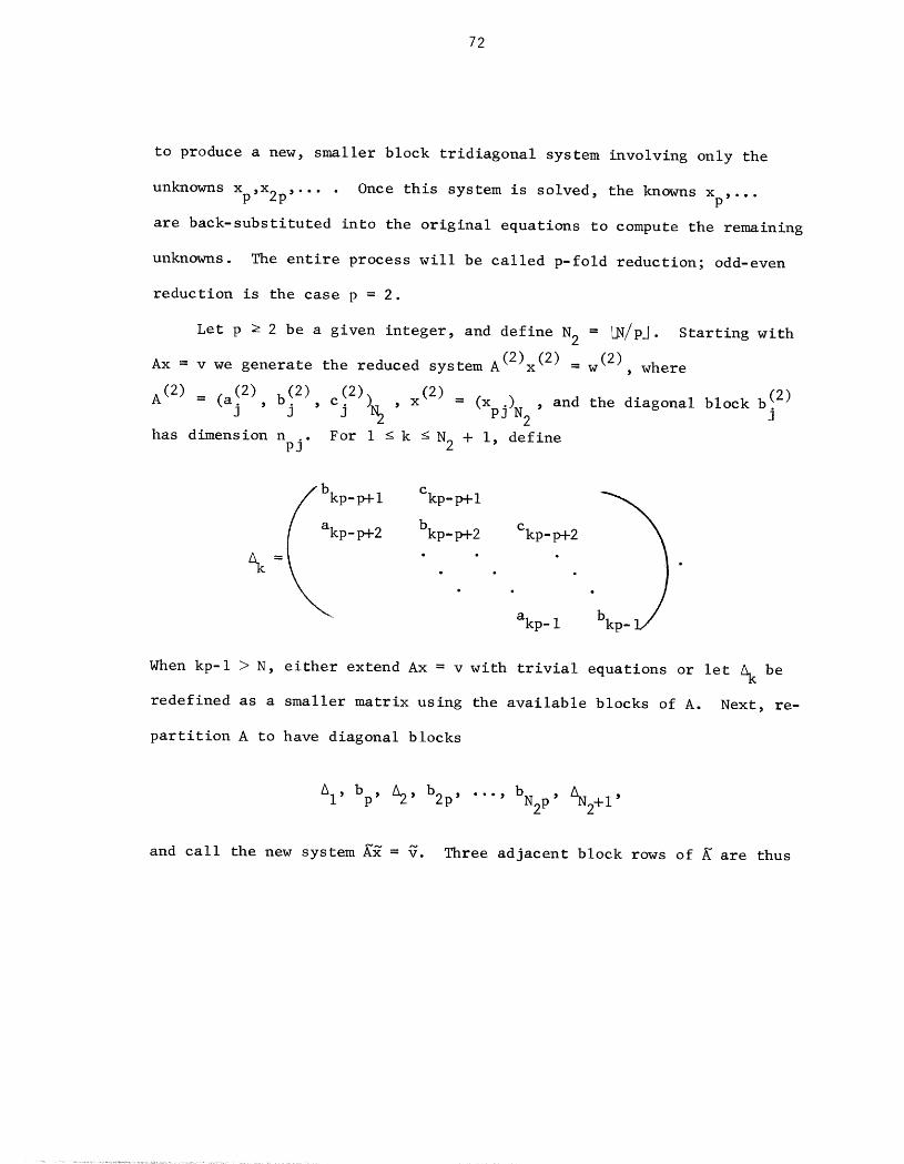
72

to produce a new, smaller block tridiagonal system involving only the

unknowns Xp,X2p, .... Once this system is solved, the knowns Xp,...

are back-substituted into the original equations to compute the remaining

unknowns. The entire process will be called p-fold reduction; odd-even

reduction is the case p = 2.

Let p _ 2 be a given integer, and define N2 = LN/pJ. Starting with

(2) whereAx = v we generate the reduced system A(2)x (2) = w ,

A (2) = (a(2)j, b(2)j, c(2))_j , x(2) = (Xpj)N2 , and the diagonal block b(2)j

has dimension n .. For I _ k _ N2 + i, definePJ

f bkp-p+l Ckp-p+l

ak_p- p+2 bkp-. p+2 . Ckp- p-t--2.akp- I

When kp-I > N, either extend Ax = v with trivial equations or let _ be

redefined as a smaller matrix using the available blocks of A. Next, re-

partition A to have diagonal blocks

AI, bp, _, b2p, ..., bN2 p, _2+i,

and call the new system K_ = v. Three adjacent block rows of K are thus

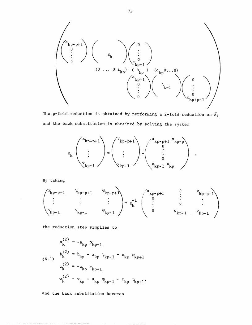
73

kSkp- I

(0 ... 0 akp) ( bkp ) (Ckp0...0)

p-

The p-fold reduction is obtained by performing a 2-fold reduction on A,

and the back substitution is obtained by solving the system

I i jakPp ixkP_-_ V_p_/ 0_ : -_o0 /_kp- I / _kp- I / kp- I Xkp

By taking

( 0/ kp- p+l :

,___ ___ ___ :_\i o_a_-_,_-_ %-_/ ___ v_._/the reduction step simplies to

ak2( ) = -akp _kp-I

bk(2) = bkp- akp _kp-I- Ckp _kp+l(6.1)

Ck2)" = -Ckp _kp+l

Wk(2) = Vkp - akp q°kp-I - Ckp _p+l'

and the back substitution becomes

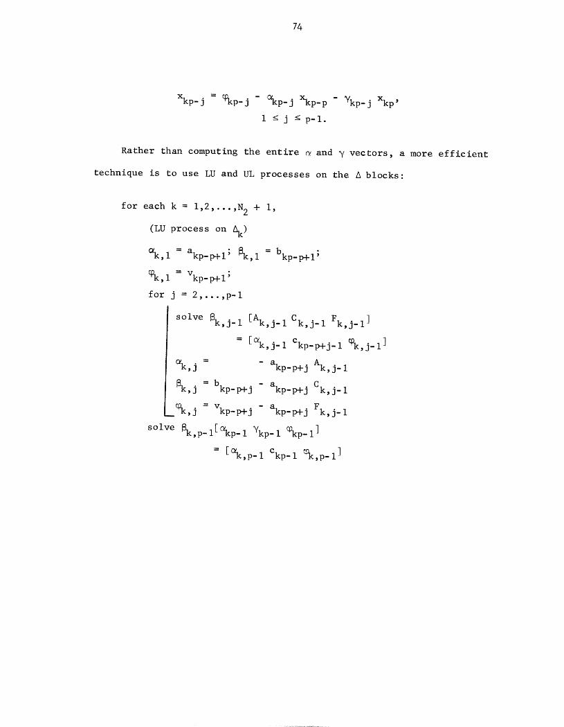
74

Xkp-j - _kp-j - _kp-j Xkp-p - _kp-j Xkp'

i <j <p-l.

Rather than computing the entire _ and _ vectors, a more efficient

technique is to use LU and UL processes on the A blocks:

for each k = 1,2,...,N 2 + I,

(LU process on _)

_k,l = akp-p+l; _k,l = bkp-p+l;

q°k,I = Vkp-p+l ;

for j = 2,...,p-I

solve Bk,j_ I [Ak,j. I Ck,j_ I Fk,j_ I]

= [_k,j-I Ckp-p+j-I q°k,j-l]

_k,j = - akp-p+j Ak,j-I

Bk,j = bkp-p+j - akp-p+j Ck,j-I

__k,j = Vkp-p+j - akp-p+j Fk,j- I

solve _k,p_l[_kp_l _fkp-I C°kp-l]

= [_k,p-I Ckp-I _k,p-I ]

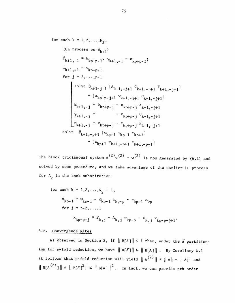
75

for each k = 1,2,...,N 2,

(UL process on _+i )

_k+l,- I = bkp+p- I; _k+l,- I = Ckp+p- I;

q°k+I,-I = Vkp+p- I

for j = 2,...,p-I

solve _k+l-j+l [Ak+l,-j+l Ck+l,-j+l Fk+l,-j+l]

= [akp+p-j+l _fk+l,-j+l _k+l,-j+l ]

_k+ I,-j - bkp+p- j kp+p- j Ak+ 1,-j+I

_fk+l,-j - - Ckp+p-j Ck+l,-j+l

.__°k+l,-j = Vkp+p- j - Ckp+p- j Fk+l,- j+l

solve _k+l,-p+l [_kp+l _fkp+l C_kp+l]

= [akp+l Yk+l,-p+l q°k+l,-p+l]

The block tridiagonal system A(2)x (2) = w (2) is now generated by (6.1) and

solved by some procedure, and we take advantage of the earlier LU process

for _ in the back substitution:

for each k = 1,2,...,N 2 + i,

Xkp-I = _°kp-I - _kp-I Xkp-p - _kp-I Xkp

for j = p-2,...,l

Xkp_p+j " Fk,j - Ak,j Xkp-p - Ck,j Xkp-p+j+l"

6.B. Convergence Rates

As observed in Section 2, if IIB[A]II < I then, under the _ partition-

ing for p-fold reduction, we have IIB[_]]I _ IIB[A]II • By Corollary 4.1

it follows that p-fold reduction will yield I]A(2) II< ]I_[II= IIAll and

IIB[A(2)]I I< IIB[_] 211 < IIB[A]II2" In fact, we can provide pth order

76

convergence, although our first result is somewhat weaker than mi_h_ _

expected in comparison to earlier results.

We will actually consider a natural generalization of odd-even elim-

ination. Let M be a nonsingular block (2p-l)-diagonal matrix,P

Mp = (mj,_p+l,...,mj,0,...,mj,p_l)N .

We want to pick M such thatP

M A =(rj, 0, ..., 0, s 0 ,0 tj)p j' , ... , •

p-I p-i

M A is a block (2p+l)-diagonal matrix; A _2_f_ is constructed by selectingP

the intersections of the block rows p,2p,..., and block columns p,2p, ....

Thus we have

(2) (2)a. = r b = s.J JP' J 3P

c(2) (2)= t.p,j w. = )J (MpV jpJ

Now, the jth block row of M A isP

vP-I

mj,k[block row (j+k) of A],_k--p+l

so that

r. = m. -p+l a3 J, j-p+l'

s. = m. cj_ + m b + m3 j,-I i j,0 j j,+l aj+l

t. =m. c .3 3,p-I j+p-I

We require that

mj,k_ I Cj+k_ I + mj, k bj+ k + mj,k+ I aj+k+ I = 0,

Ikl = 1,2,...,p-l,

77

where we take m° = 0, m. = 0.J,-P 3,P

The special case p = 2, Mp = (-ajbill_ l,-cjbi+-, i), has been considered

in Section 4.A. For p > 2, define

d. -- b

j,-p+l j-p+l

d =b - a di_j,-k j-k j-k -k-I Cj-k-l'

k = p-2,...,l

-I

_j,-k = -aj-k dj,-k-l'

k = p-2,...,0

d =bj,p-i j+p- I

dj,k = bj+k - cj+k dil,k+l aj+k+l'

k = p-2,...,l,

_j,k = -cJ +k dil,k+l'

k = p-2,...,0.

Then we may take

mj,_k = _j,0 _j,-I "'" _j,-k+l

mj, 0 = I

mj,k = _j,0 _j "'" _,I j,k-l'

k = 1,2,...,p-I.

! !

The dj,_k s are derived by an LU factorization process, and the dj,+k s

by a UL process. It follows from earlier results that if IIC[A]III < i

then IImj,+klIl _ IIC[A]IIkI ' so the diagonals of M decrease in size as one_ P

moves away from the main diagonal.

Our first theorem partially generalizes Theorem 4.1.

78

-I -I - icTheorem 6.1. Let J = (-sj rj, 0, ..., 0, -s.j t.),j B = (-bj aj,0,I -b-j j),

B = L + U, J = JL + Ju' IILII _ _, IIUll _ _, IIBII _ 2_ = _, with _ _i2"

Then IIJll _ _P, IIjLII _I_ p, lljull _I_ p.

Proof. Let R0 - 0, _ = L(I- Rk_I)'Iu, TO = 0, Tk = U(I- Tk_I)'IL,

k = l,...,p-l, S = R + T so thatp-I p-l'

(I - S)JL = L(I - Rp_2)'IL(I - R 3)-IL ... L(I - R0)-ILp-

(I - S)JU = U(I- T 2)'Iu -Iu -IUP- (I- T 3) ... U(I- TO) .p-

2 -I

Define _0 = 0, _k = _ (I - ,k_i) , so

II _ *k' IITkll*k'

I IIJ ll _/[<_ - 2_p_i)_-20 (i - ,k)],

IIJll _ I_P/[2p-I( 1 - 2,p_1)II_-20(1 - _'k) ].

= = - 26k_ so 6k det(_,l _)(k_l)×(k_l)> 0Define 60 0, 61 I, 6k+I - 6k - _ I' = '

_k = _26kI/6k+l' I - _k = 6k+2/6k+l' (i - 2,p_l )_-20(I - ,k) =2 2

(I - 2_p_l )6p = 6p+l - _ 6p_l. Define Tk = 6k+l - _ 6k-l' so T1 = I,

= _ 2 , (I 2-k+lT2 I - 22, Tk= Tk-I _ ¢k-2" By induction Tk ) = ,

dT ¢_=-2_k6k-i _ 0. But then, for _ < _, ¢k(_) e Tk ), so 2P-ITp(_) e 1.

Thus IIJll < _P and IIJLII , IIJUII _ l_p. QED.

i

Corollary 6.1. If IIB[A]]I< 1, IIL[B[A]]II, IIU[B[A]]il_711B[A]il, then

II B[A(2)]II _ IIB[A]II P.

In generalization of Theorem 4.4, there is the very surprising

Theorem 6.2. With X(i) = X(A(i)), X(I) _ I, _(i) = (l__/__x(i))/(l+_/l_X(i))_,

we have

79

2 I + _(i) "

Proof. It suffices to consider i = I, so we will drop the superscripts.

= b-I dj _j = b"IDefine cj,-k j-k ,-k' ,k j+k dj,k, k = 0,...,p-l, so that

_ I. m

_. = (-a. ¢-I i) -I aj_ ¢jl I e I I)] ] J,- (-bj_l I ,_2) ... (-bj_p+2 aj-p+2 j,-p+

X (bjlp+l. aj_p+l ),

(2) = ra. jp']

tj (-cj _._l)(-bjl I cj+ I _.I ) .. -I= " ,2 " (-bj+p_2 Cj+p_2 _ _p- 1)

-1

X (bj+p_l aj+p_l )'

c (2) = t ,] ]P

b (2) = s ,J JP

- - _-.1 b-1b - a. e 1 b j_1 c j_ - cs"=] j ] j,-I I I j j,l j+l aj+l

= b.(I- (_.).] ]

Now, II_'_p_l II--i, II_;l,kll _ (I - _II_.l,k+lll/4) -1 =. By defining E1 i,

Ek (I %Ek_ i/4) I I= - - , we have II_.,p_kll < Ek Similarly ;I¢ii• , ,_p+kll _ Ek.

This yields II(:jll_ XE 1/2 II(I - -ip_ qj) II_ 2/(2 - %E I) . To bound k(2), p- '

observe that

411 b(2)-la(2)II IIb(2)-I-(2)IIj j j-I cj-I

a IIII 111II II]p ]p jp p,- p-I ajp. l

xII II II IIIIuiljp,-2 "'" jp,-p+l p-p+l ajp'p+lll

- " c. II II _'p_p,lll II jp-p+l Cjp-p+lX II (I C_jp_p) Iii IIb'.]p_pl]P-P I b-I II

p-p,2 "'" p-p,p- 1 jp-I Cjp-I

4 XE (_)P iqp'l_ 3=i J "p-

80

Thus 4(2) is bounded by the above quantity. Suppose first that X = I,

which implies that _ = 1. Then E = 2n/(n+l), the bound simplifies ton

Xp, and we are done with this case. Now suppose that _ < I. It may be

n+l) ,shown by induction that E = (I + _)(I - _n)/(l - _ yieldingn

(2/(2 - XE 1))2= (i - X)'I((I - _P)/(I + _p))2 and with a little effortp- _

the bound simplifies to the desired result. QED

Note that we have not actually shown that %(i) < I implies x(i+l) < I.

This point is now to be resolved.

Corollary 6.2. If x(i) _ I then %(i+l) < %(i)p with strict inequality if

(i+l) (i)p_(i) < I, and _ -<_ .

Proof. The case %(i) = 1 was considered in Theorem 6.2. Suppose that

0 _ % < I, again considering only the case i = i. It is not hard to show

_/2J i

that ((I + _)/2)P(2/(I + _P)) = (_p(X))-l, where _p(X) = (Pi)(l - _) .i=0

Now, _p(1) = I, _p(X) < 0 for 0 _ _ < I, so he(X ) > i for 0 < _ < I and

X(2) < xp for this case. Assuming only _ _ I, and since _(I + _)2/4 = _,

we have 4(2) _ _P(2/(I + _p))2, which implies _(2) _ _p. QED

6.C. Back Substitution

Error propagation in the back substitution for p-fold reduction de-

pends on the particular implementation. In the simplest form

Xkp-j = q°kp-j - _kp-j Xkp-p - Ykp-j Xkp'

errors in Xkp_j depend on newly generated rounding errors and propagated

and . We can write the computed solution aserrors from Xkp_p Xkp

Ykp-j = Xkp-j + _kp-j to find

81

_kp-j = -_kp-j _kp-p - _kp-j _kp + ¢kp-j"

It follows from the analysis of the Gauss-Jordan algorithm (Corollary 3.5)

and from explicit formulae for _kp-j' _kp-j' that II_kp_jll < IIB[A]I_ -j,

II_kp_jll _ IIB[A]I_ if IIB[A]II < I, which leads to

II_kp-jll < IIB[A]I_-Jll _kp-pll + IIB[A]I_II _kpll+ IIekp_jll.

Errors in a newly computed component therefore depend most strongly on

errors in its closest back-substituted component, and the "influence"

decreases as the distance between components increases. Moreover, we

have

II_kp_jll _ IIB[_]II max(ll _kp.pll, II_kpll)+ IIekp_jli.

If e is a bound on errors introduced at each stage, it follows that errors

in the final computed result will be bounded by ¢ logp N.

Slightly different results prevail in the back substitution

Xkp-I = _kp-I - _kp-I Xkp-p - _kp-I Xkp

for j = 2,...,p-I

Xkp_j = Fk - Ak - Ck,p-j ,p-j Xkp-p ,p-j Xkp-j+l

Errors in the computed solution Ykp-j = Xkp-j + _kp-j obey the rule

_kp-I = -_kp-i _kp-p - Vkp-p _kp + ekp-I

for j = 2,...,p-I

_kp-j = -Ak,p-j _kp-p- Ck,p-j _kp-j+l + ekp-j'

and ratherso the errors in Xkp_j depend on propagation from Xkp_p Xkp_j+l

than Xkp_p and Xkp. This implies a linear growth as in the LU factorization

82

in conjunction with logarithmic growth as in odd-even reduction. If we

again suppose that IIekp_jll _ ¢, with I]_kp_pll, I[_kpl] _ _, it follows

that

II_kp-I [I_ IIB[K]II _ + ¢,

]]_kp_jl[ _ IIB[K]II max(_, I[gkp_j+ll[ ) + ¢

which leads to II_kp_jll _ _ + (p-l) e. The end result is that errors in

the final computed result will be bounded by cp logp N.

83

7. SEMIDIRECT METHODS

Briefly, a semidirect method is a direct method that is stopped be-

fore completion. In common usage, a direct method for the solution of

Ax = v computes x exactly in a finite number of steps if exact arithmetic

is used, while an iterative method computes a sequence of approximations

x (i) converging to x. The semidirect methods are intermediate on this

scale, producing an approximation to x in a finite number of steps,

while an additional finite number of steps could produce x exactly. During

the computation, intermediate results are generated which approximate the

solution. If the error is small enough then the algorithm is terminated

prematurely and an approximate solution is returned.

The method of conjugate gradients is an example of a semidirect

method since it can produce a good approximation long before its usual

termination [R2]. The accelerated Parallel Gauss iteration ([H4] and

Section 8.E) is another example, as is Malcolm and Palmer's convergent LU

factorization [M2] of A = (a,b,a), a and b positive definite with 0(b-la) < i.

Here we consider semidirect methods based on the quadratic conver-

gence properties of the odd-even methods. This will generalize various

results obtained by Hockney [H5], Stone [S2] and Jordan [Jl]. Buzbee [BI7]

discusses a similar technique based on the Buneman algorithm for Poisson's

equation (cf. Theorem 4.3).

The name semi-iterative has already been appropriated for other purposes

[V3]. Stone [$2] initiated the name semidirect.

84

7.A. Incomplete Elimination

Let us first consider odd-even elimination for Ax = v, which is the

process H I = A, v (I) = v, Hi+ I = (I + C[Hi])Hi, v(i+l)= (I + C[Hi])v(i).

In Theorem 4.1 we proved that if IIB[A]II < I then IIB[Hi+ I]II _ IIB[H i]211,

so that the off-diagonal blocks decrease quadratically in magnitude rela-

tive to the diagonal blocks. This motivates the approximate solution

Z (i)D[Hi]'Iv (i). Because we halt the process before completion, we

call this technique incomplete odd-even elimination.

Theorem 7.1. IIx - z(i) II/II xll < IIB[Hi]ll"

Proof. Since v(i) Hl= .x = D[Hi](l- B[Hi])x we have z(i) = D[Hi]-Iv (i) =

x - B[H i]x. QED

Thus the B matrix determines the relative error in the simple approxi-

mation z(i). If B = IIB[A]II < I, 0 < e < I, m = Flog2 hi, then

(7.I) k = I + max(0, min(m, °g2 _og----_ ))

I -20

guarantees IIB[Hk]II _ ¢. For example, if 8 = _, ¢ = 2 - 10-6 , then

k = 6 and we should have N > 32 for incomplete odd-even elimination to be

applied. In fact, IIB[H kill < 825 = 2.32 - I0-9"6, so the results of the

incomplete elimination would be much better than required.

In the case n = I, a. = c. = a, b. = b, we have IIB[Hi+l]ll =J J J

2 x 2 x 2]]B[Hi ]211/ (2 - IIB[Hi]211 ). Since x /2 < x2/(2 - ) < for 0 < x < I,

k must be larger than

(7.2) i + l°g211°gmog2(8/2(e/21

85

2k-Iin order to have IIB[Hk]II _ ¢. (By induction, B(k) > 2(B/2) , and if

2k-I2(_/2) > c then _(k) > ¢.) A more refined lower bound is obtained

by defining T 1 = _, Tn+ 1 = T2n/(2 - T2)n' and computing the largest k such

that

(7.3) Tk > ¢.

Since B[Hi] is the matrix associated with the block Jacobi iteration for

H.xl = v(i)' when IIB[Hk]II is small we can use this iteration to improve

g(k)In fact the choice z(k) = D[Hk ]-I is the iterate

the estimate

(k) (k,0)following the initial choice z = 0. If z is an approximation to

(k,i+l) (k i) -Iv(k )x and z = B[H k]z ' + D[Hk] then [[x - z(k'£) [[

(k,0)][B[Hk]_II [Ix - z I]• k and _ may now be chosen to minimize computa-

B2k- Ition time subject to the constraint _ _ e. Any of the other standard

iterative methods may be used in place of the Jacobi iteration; for related

results using the theory of non-negative matrices and regular splittings,

see [HI].

We have remarked earlier that if the tridiagonal matrix A = (aj, bj, cj)

is irreducibly diagonally dominant and _(i) = IIB[Hi]II then B(1) < I and

_(i+l) < B(i)2. This is a case of practical importance in differential

equations. However, the example A = (-I, 2, -I), for which _(i) = I,

I _ i < m-l, _(m) = 0, shows that strict inequality is necessary for incom-

plete elimination to be effective.

Indeed, when _(I) is very close to I, as will be the case for most

second-order boundary value problems, the fact that we have strict in-

equality does not imply that _(i) will be small for i < m. With regard

-I (i) (i)to the particular approximation z (i) = D[Hi] v , z. depends only onJ

v_, j - (2i-I - I) _ _ -<j + (2 i-I + I). Thus for N = 2m - I, i < m,

86

(i) ,

the center point Z2m_l will be independent of the boundary data. Al-

though this is not the only possible approximation, complete odd-even

elimination will be necessary to ensure convergence to the continuous

solution.

7.B. Incomplete Reduction

The incomplete odd-even reduction algorithm is analagous to incomplete

odd-even elimination. Complete reduction generates a sequence of block

tridiagonal systems A(i)x (i) (i)= w , i = l,...,m, m = Flog2 N + 17, solves

A(m)x (m) = w (m) exactly for x (m) , and back substitutes to finally obtain

x = x (I) . Incomplete reduction stops with A(k)x (k) = w (k) for some k be-

(k) x (k) and backtween 1 and m, solves this system approximately for y _ ,

(i) (i)substitutes y(k) to obtain y = y _ x .

We remind the reader of observations made in Section 4.D, especially

that roughly half the actual work is performed in the first reduction, one

quarter in the second, and so forth. Thus the savings in incomplete reduc-

tion would be much less than those in incomplete elimination, where the

work per step is roughly constant. For more details, see Section 10.C.

In contrast to incomplete elimination, the incomplete reduction must

deal with error propagation in the back substitution. We have already

shown that roundoff errors in complete reduction are well-behaved, and

can only grow at most logarithmically. But since the approximation errors

quite possibly might be larger than the roundoff errors, a different analy-

sis is needed. We will see that a number of interesting properties result,

including no growth of errors under certain assumptions about roundoff,

This observation is due to an anonymous referee of [H2].

87

and a superconvergence-like effect due to damping of errors•

(k)An initial approximation y(k) may be computed from A (k) and w ac-

cording to our analysis of incomplete elimination. The choice

(k) (k) - lw(k) (k) (k) (k)y = D[A ] is a simple one, and we have l_(k)-y IPI_ II< I_[A ]ll-

The parameter k should be determined both for computational economy and

for a suitable approximation• Here the quadratic decreases of B[A (i) ] are

important and useful in some (but certainly not all) situations.

(k) let us supposeRegardless of the source of the approximation y ,

y_k)- = x (k).+ 6(k).. In the back substitution, y(i) is computed fromthat

J J

y (i+l) by

i) (i+l)Y_j = Yj

y_i) = ib(i) -i. (i) a(i) (i+l) c(i) (i+l) (i)j-i " 2j-I ) tw2j-I- 2j-I Yj-I - 2j-I Yj ) + e2j-l'

with ¢ j-1 representing rounding errors, We then have

8(i) (i+l)2j = 6.J

6(i) = ¢_i) _ ib(i) l)-I o(i) $(i+I) + c_i) 6(i+I))2j-I j-I " 2j- (a_j-I -j-i j-i j "

Theorem 7.2. If II¢(i)II < (i - IIB[A(i) ]II> II6(i+I)II then I16(i) II: II6(i+I) II"

Proof. By construction,

o

i, •

88

As in the analysis of roundoff error propagation for complete odd-even

reduction, we have

II6(i) II_ max(ll 6(i+I)II, II¢(i)II+ IIB[A(i) ]II II6(i+i)II )"

From this expression and the hypothesis we have II6(i> II< II$(i+I)II •

But, also by construction, II8(i) II_ II6(i+i)II • QED

This theorem requires some explanation. First suppose that no round-

ing errors are committed, so that ¢(i) = 0 and all the error in y(1) is

(k)derived from the approximation error in y . It now follows from

IIB[A]II < I that this error will not grow during the back substitution.

(k) (k)From IIx(k) II< IIxll , we conclude that I_-Yll/I_II < l_(k)-Y II/l_ II°

In fact, it is easy to see that while IIx- Y ll= IIx(k) - y(k)If, many

vector components of x-y will be much smaller in size than IIx- Yll •

In Figure 7. I we illustrate the errors by component for the tridiagonal

system (-I, 4, -l)x = v, N = 31, k = m-I = 4, v chosen so that x. = I,J

and yj-(k)= b(k)-lw(k)jj . In the absence of rounding errors, the back sub-

stitution quickly damps out approximation errors, creating a very pleasing

super convergence- like effect.

Now suppose that rounding errors are committed and we have the upper

bound II¢(i)II < ¢- If II6(k) II< v¢ for some moderate constant _ then we

have essentially solved the system A(k)x (k) = w (k) exactly, and the error

propagation analysis is the same as for complete reduction. That is, we

have II8(i) II< (k - i + _)e, I < i _ k.

The remaining case is when II8(k) II>> ¢- Here the semidirect method

must be considered in competition with an iterative method. The hypoth-

esis of Theorem 7.2, II6(k) II(i - IIB[A(k)]ll) _ ¢, should be viewed as

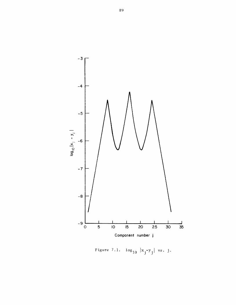
89

-3

-4

-5

m

I

._ _ 6

X

£)

¢=m0

-7

-8

-9 I I I i I J0 5 I0 15 20 25 30 35

Component number j

Figure 7.1. togl0 Ixj-yjl vs. j.

90

an attempt to formalize the condition II6(k) II>> ¢- As long as the hypoth-

esis remains true, the difference (in norm) between x (i) and y(i) can en-

tirely be attributed to the original approximation error. As soon as the

hypothesis is violated it is possible for the errors to grow, but we will

still be able to say that IIx - Yll = II6(k) II+ O(ke). Although the super-

convergence effect would be moderated somewhat by roundoff, its qualitative

effects will still be felt and we can expect this bound on accumulated er-

ror to be an overestimate.

7.C. Applicability of the Methods

We close with some remarks on the practical application of the qua-

dratic semidirect methods. In Buzbee's analysis [BI7] of the Buneman algo-

rithm for the differential equation (-A + d)u = f on a rectangle with

sides _I and _2' d a nonnegative constant, it is shown that if

i

_I 2 _2 ]_cq [d_2 + >> 1

then a truncated Buneman algorithm will be useful. Geometrically this re-

quires that the rectangle be long and thin if d is small, and hence the

block tridiagonal matrix will have small blocks when properly ordered.

By directly considering the finite difference approximation to Poisson's

equation on a rectangle with equal mesh spacing in both directions it is

possible to reach a similar conclusion; this also serves as a simple model

for more general elliptic equations. With M nodes in one direction and N

in the other, M < N, the matrix A is (-_, PM' -_)N' PM = (-I, 4, -I)M.

It is readily verified that IIB[A]II = 211 QMII , QM = PMI'

91

I D + D I-

_(I- m m-D ) _ n=2m'n

I_nll= 2DI m

"_'(1 - "_'), n = 2re+l,I1

DO =4 D =4 D - D .= I, D1 ' n n-I n-2

The following table gives IIB[A]II for M = 1(1)6, along with estimates

on the number of odd-even reductions needed to obtain IIB[A(i) ]II< 10"8"

k such that IIB[A(k) ]ll< I0-8

M IIB[A]II lower bounds upper bound(7.2) (7.3) (7.1)

w

II - = .5 5 5 6

2

2 2 -.67 6 6 73

3 6 .- = .86 6 7 87

I04 - .91 6 7 9

II

5 25 _ .96 6 8 I026

6 40 . .98 6 8 II41

These figures again lead to the conclusion that the best use of the semi-

direct methods for elliptic equations will be with long thin regions. In

the next section we consider some iterative methods which use matrix split-

tings and orderings to take advantage of this property.

92

8. ITERAT IVE METHODS

In this section we consider the iterative solution of a finite dif-

ference approximation to a general nonseparable elliptic equation. Of

particular interest will be methods which employ, as part of each itera-

tive step, the direct or semi-direct solution of a block tridiagonal

linear system. Continuing our emphasis on methods for a parallel computer,

we want this system to be such that the method already considered can be

used efficiently.

8.A. Use of Elimination

Let us first note that several of our theorems about block elimination

have applications to iterative methods. Consider the system Ax = v and

(i+l) ix(i) Ithe block Jacobi iteration x = B[A + D[A]- v. Suppose that

[[B[A][ I< I, so the iteration converges; this condition is satisfied for

many elliptic equations with suitable partitioning IV3]. If the structure

of A can be simplified by an elimination step, forming A'x = v', then

subsequent computations will be handled more efficiently, and since

IIB[A' ]II< IIB[A]II the iteration will not converge any slower.

Indeed, convergence of the block Jacobi iteration will often be quite

slow. When A is also positive definite the Jacobi semi-iterative method

(J - Sl or Chebychev acceleration) IV3]

(i+l) (B[A]x(i) -i (i- 1)) (i-l)x = _i+l + DIAl v- x + x ,

_I = I, v2 = 2/(2- 02),

Vi+ I (I - 02Vi/4) - I= , 0 = 0(B[A]),

will converge at a much faster rate and is a natural candidate for parallel

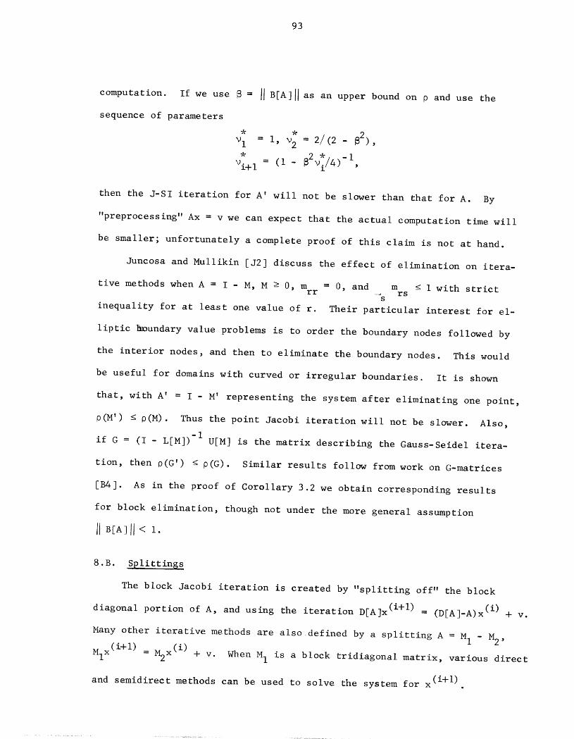
93

computation. If we use _ = IIB[A]II as an upper bound on P and use the

sequence of parameters

* * _2)Vl = I, v2 = 2/(2 - ,

* _2 * -_i+l = (I- vi/4 ) I,

then the J-SI iteration for A' will not be slower than that for A. By

"preprocessing" Ax = v we can expect that the actual computation time will

be smaller; unfortunately a complete proof of this claim is not at hand.

Juncosa and Mullikin [J2] discuss the effect of elimination on itera-

tive methods when A = I - M, M e 0, m = 0, and m _ I with strictrr .... rss

inequality for at least one value of r. Their particular interest for el-

liptic h_undary value problems is to order the boundary nodes followed by

the interior nodes, and then to eliminate the boundary nodes. This would

be useful for domains with curved or irregular boundaries. It is shown

that, with A' = I - M' representing the system after eliminating one point,

p(M') < 0(M). Thus the point Jacobi iteration will not be slower. Also,

-Iif G = (I - L[M]) U[M] is the matrix describing the Gauss-Seidel itera-

tion, then 0(G') < o(G). Similar results follow from work on G-matrices

[B4]. As in the proof of Corollary 3.2 we obtain corresponding results

for block elimination, though not under the more general assumption

IIB AIII<

8.B. Splittinss

The block Jacobi iteration is created by "splitting off" the block

diagonal portion of A, and using the iteration D[A]x (i+l) = (D[A]-A)x (i) + v.

Many other iterative methods are also defined by a splitting A = M 1 - M2,

MlX(i+l) = M2x(i) + v. When M 1 is a block tridiagonal matrix, various direct

(i+l)and semidireet methods can be used to solve the system for x

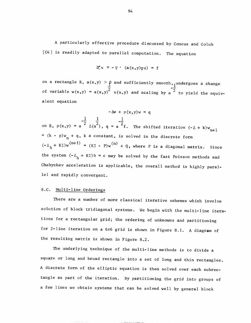
94

A particularly effective procedure discussed by Concus and Golub

[C4] is readily adapted to parallel computation. The equation

_u = -V " (a(x,y)vu) = f

on a rectangle R, a(x,y) > _ and sufficiently smooth,lundergoes a change

y)2 2of variable w(x,y) = a(x, u(x,y) and scaling by a to yield the equiv-

alent equation

-Aw + p(x,y)w = q

I i I

2 A(a2 2on R, p(x,y) = a ), q = a f. The shifted iteration (-A + k)Wn+ I

= (k - p)w n + q, k a constant, is solved in the discrete form

(-Ah+ Kl)w (n+l) = (KI - P)w (n) + Q, where P is a diagonal matrix. Since

the system (-A h + Kl)b = c may be solved by the fast Poisson methods and

Chebychev acceleration is applicable, the overall method is highly paral-

lel and rapidly convergent.

8.C. Multi- line Orderinss

There are a number of more classical iterative schemes which involve

solution of block tridiagonal systems. We begin with the multi-line itera-

tions for a rectangular grid; the ordering of unknowns and partitioning

for 2-1ine iteration on a 6×6 grid is shown in Figure 8.1. A diagram of

the resulting matrix is shown in Figure 8.2.

The underlying technique of the multi-line methods is to divide a

square or long and broad rectangle into a set of long and thin rectangles.

A discrete form of the elliptic equation is then solved over each subrec-

tangle as part of the iteration. By partitioning the grid into groups of

a few lines we obtain systems that can be solved well by general block

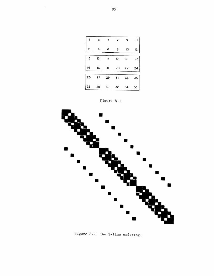
95

I 3 5 7 9 II /

J2 4 6 8 I0 12

13 15 17 19 21 23

14 16 18 20 22 24

25 27 29 31 33 35

26 28 30 32 34 36

Figure 8.1

1

I

I

1

1

1 1

1 1

1 1

1 1

1 1

1 1

1 1

11

1

1

1

Figure 8.2 The 2-1ine ordering.

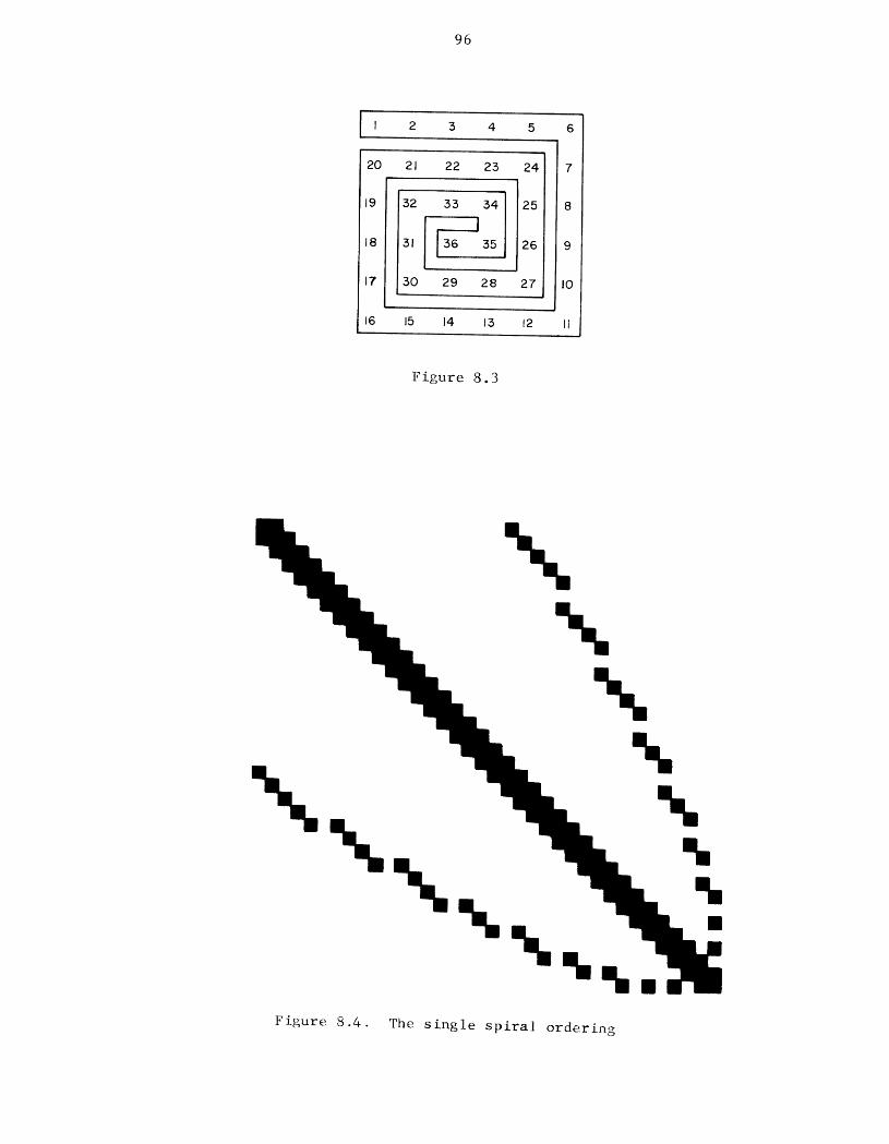
96

I 2 3 4 5 6

20 21 22 2.3 24

19 32 33 34 25r------'--I

I8 31 I 36_ 35 26

17 30 29 28 27

t6 15 14 13 12 II

Figure 8.3

Figure 8.4. The single spiral ordering

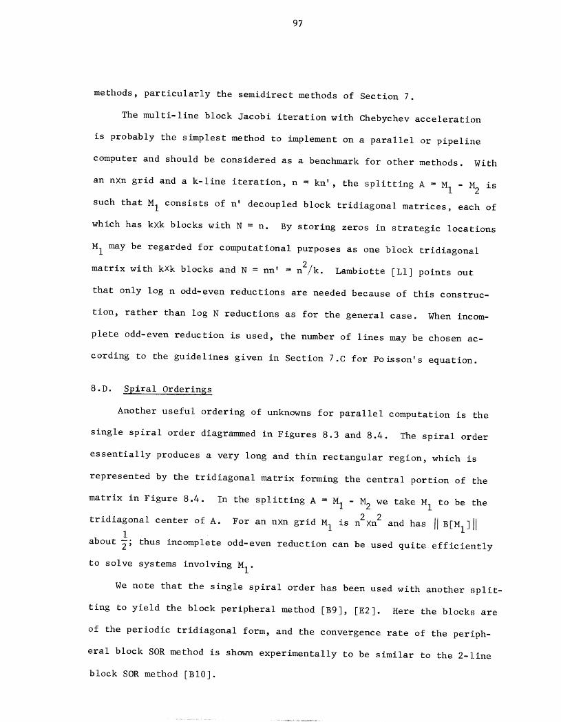
97

methods, particularly the semidirect methods of Section 7.

The multi-line block Jacobi iteration with Chebychev acceleration

is probably the simplest method to implement on a parallel or pipeline

computer and should be considered as a benchmark for other methods. With

an n×n grid and a k-line iteration, n = kn', the splitting A = MI - M2 is

such that M I consists of n' decoupled block tridiagonal matrices, each of

which has k×k blocks with N = n. By storing zeros in strategic locations

MI may be regarded for computational purposes as one block tridiagonal

matrix with k×k blocks and N = nn' = n2/k. Lambiotte ILl] points out

that only log n odd-even reductions are needed because of this construc-

tion, rather than log N reductions as for the general case. When incom-

plete odd-even reduction is used, the number of lines may be chosen ac-

cording to the guidelines given in Section 7.C for Poisson's equation.

8.D. Spiral Orderings

Another useful ordering of unknowns for parallel computation is the

single spiral order diagrammed in Figures 8.3 and 8.4. The spiral order

essentially produces a very long and thin rectangular region, which is

represented by the tridiagonal matrix forming the central portion of the

matrix in Figure 8.4. In the splitting A = MI - M2 we take MI to be the

2 2

tridiagonal center of A. For an nXn grid MI is n ×n and has IIB[MI]III

about _; thus incomplete odd-even reduction can be used quite efficiently

to solve systems involving MI.

We note that the single spiral order has been used with another split-

ting to yield the block peripheral method [B9], [E2]. Here the blocks are

of the periodic tridiagonal form, and the convergence rate of the periph-

eral block SOR method is shown experimentally to be similar to the 2-line

block SOR method [BI0].

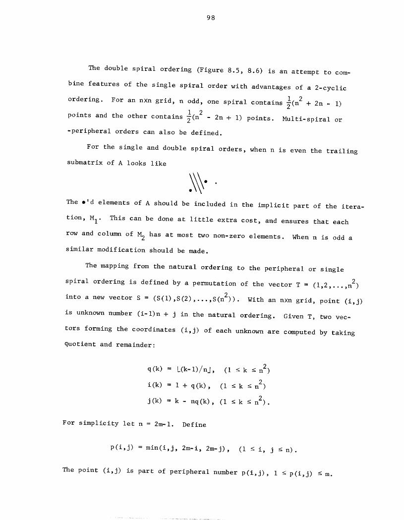
98

The double spiral ordering (Figure 8.5, 8.6) is an attempt to com-

bine features of the single spiral order with advantages of a 2-cyclic

1 2

ordering. For an n×n grid, n odd, one spiral contains _(n + 2n - I)1 2

points and the other contains _(n - 2n + I) points. Multi-spiral oi:

-peripheral orders can also be defined.

For the single and double spiral orders, when n is even the trailing

submatrix of A looks like

The e'd elements of A should be included in the implicit part of the itera-

tion, M I. This can be done at little extra cost, and ensures that each

row and column of M2 has at most two non-zero elements. When n is odd a

similar modification should be made.

The mapping from the natural ordering to the peripheral or single

spiral ordering is defined by a permutation of the vector T = (1,2,...,n 2)

into a new vector S = (S(1),S(2),...,S(n2)). With an n×n grid, point (i,j)

is unknown number (i-l)n + j in the natural ordering. Given T, two vec-

tors forming the coordinates (i,j) of each unknown are computed by taking

quotient and remainder:

q(k) = L(k-l)/nj, (I _ k < n2)

i(k) = I + q(k), (I _ k < n2)

j(k) = k - nq(k), (I _ k _ n2).

For simplicity let n = 2m-l. Define

p(i,j) = min(i,j, 2m-i, 2m-j), (i _ i, j < n).

The point (i,j) is part of peripheral number p(i,j), I _ p(i,j) _ m.

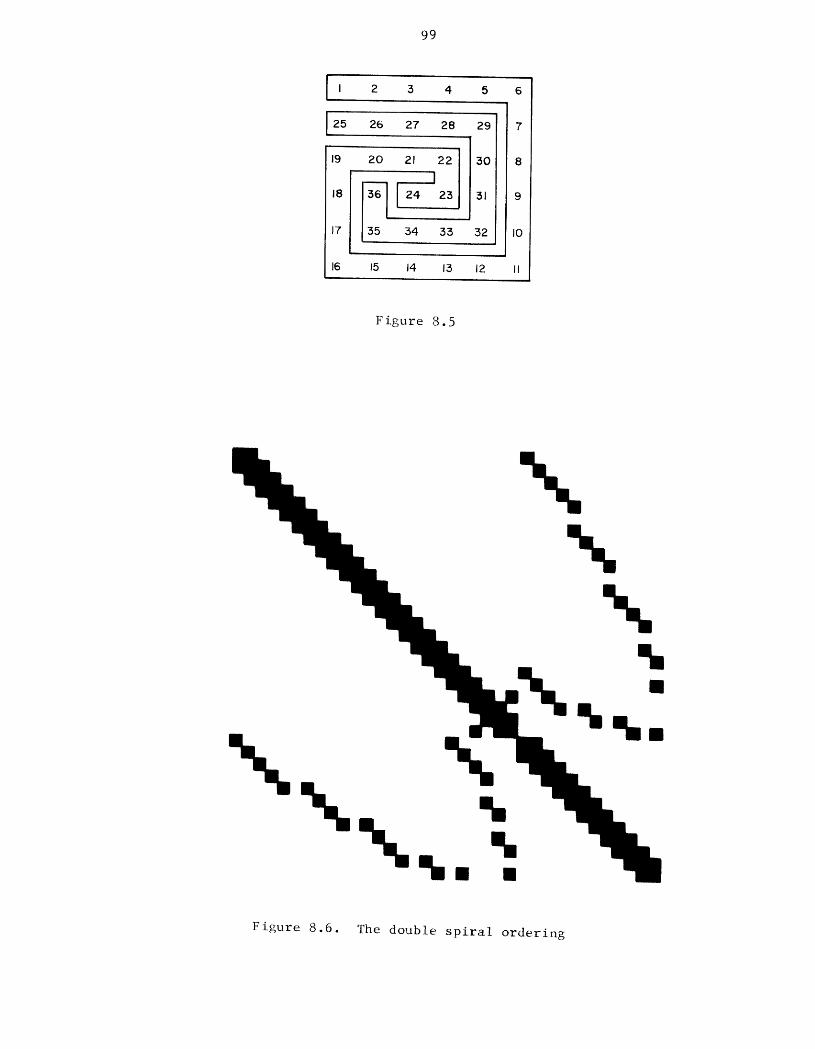
99

I 2 3 4 5 6

25 26 27 28 29 7

19 20 21 22 30 8

J

18 _]36 I I,, 24 2_ 31 9

17 1,35 I _4 33 32 I0

16 15 14 13 12 II

Figure 8.5

Figure 8.6. The double spiral ordering

IO0

Peripheral p has 8(m-p) points in it, except for peripheral m which con-

tains the single point (m,m) .

The peripheral ordering is per. I, per.2, ..., per. m, where each

peripheral is taken in clockwise order: top, rhs, bottom, lhs. Define

p-I

f(i,j) = _k=l 8(m-k) = 4(2m-p)(p-l),

the number of elements contained in peripherals 1,2,...,p(i,j) - I, and

g(i,j) = f(i,j) + I (i-p) + (j-p) + i if i < j,

8(m-p) - (i-p) - (j-p) + I if i > j

= 4p(2m-p) + I -8m + (if i _ j) (2p + i + j).

- (if i> j)

The vector S(k) = g(i,j) defines the necessary permutation, and can be

easily evaluated on a parallel or pipeline computer. The actual reordering

of a vector may be performed on the CDC STAR by using the built-in vector

permute instructions, though these should be used sparingly since they are

quite expensive. Once the vector S is generated, the elements of A and v

may be generated directly.

Of course, the implementation of an iterative method based on an

"unnatural" ordering involves much more developmental attention than is pre-

sented here. We only mean to show the potential for parallel computation.

A more complete comparison based on actual machine capabilities has not

been performed. For such a discussion of some other methods, see Lambiotte

ILl].

I01

8.E. Parallel Gauss

We close our section on iterative methods for block tridiagonal sys-

tems with some brief remarks on the Parallel Gauss iteration due to Traub

IT2] with extensions by Heller, Stevenson and Traub [H4]. For simplicity

we consider the normalized form A = (aj, I, cj).

In the block LU factorization A = (£j, I, 0)(0, dj, cj), let

D = diag(dl,...,dN). Since D = I - L[A]D-Iu[A], a natural parallel itera-

tion is D (i) = I- L[A](D(i'I))-Iu[A], where D (0) is some initial estimate

of D. This forms the first of three iterations making up the Parallel

Gauss method; the other two parts are Jacobi iterations for the L and U

block bidiagonal systems. It is shown in [H4] that, with k(A) < i,

_(A) = (I - _)/(I + _), we have ]ID- D (i) II_ _II D- D (i-l) II•

Techniques for reducing the constant _ are given in [H4]. As Stone [S2]

points out, this linear convergence is much less attractive than the qua-

dratic convergence of odd-even reduction. However, in certain situations

(parabolic equations or the multi-line iterations discussed here) it is

necessary to solve a sequence of related problems, and this would hope-

fully provide suitable initial estimates.

Let A' = (a'.],I, c')] and suppose that D' has already been computed

Since d' - d = a dj I cj - a'(d_ i) Ic'j j j -I -I j - j-l' by Theorem 3.4

]Id' - d I]< (_(_ 2 ) 4' 2 )j j + ^_ + (4"-)(I+ _F

i

: _ +

Thus ]ID' - DII : maxj] Id'.]- djlI -<I - }(_I_--_-%+ I-_-_F), and we may take D'

as an initial approximation to D. Now, the Parallel Gauss iteration is

102

most useful when X and X' are not too close to i, and in this case good

initial approximations will be available by the above bound on IID' - DII.

When X and X' are close to 1 the bound will be large, but in this case

the iteration should probably not be used due to slow convergence.

For tridiagonal matrices we have

dI = 0' _ dI

-I -I

d'.- d = a (d_ I) (dj. - d l)dj cjJ j j - I j- -I -I-I

- a'. c'. i)+ (d _i ) (aj cj_ I J J- ,

so that

]d' - d ] < I- _/_ d'. - d ,I+2

J J 1 + _,l-/Tf_ I J-1 j-1 1 + _ ]ajcj-1 - a'.c' I3 j-1 "

-a'c' ] _ (X + _')/4, 6j J JLet A = maxjlajcj_ 1 j j-I = Id'- d [,

a = (i - 1,,_-X)//(1 + Ji'_), b - 2/(1 + _/_--_) . Then hI - 0, 6j < a 8j_ 1 + b,

so by induction 6. < (1 + a + ... + aJ-2)b < b/(l-a) or 5 _ 2_/(^/_'-X + ,,_)J ' .J° •

By the intermediate value theorem (I_'X-X + ^/rf2"_)//2 ,_I-_X* for some k*= be-

tween _. and X' , so that 5. < A/_ . Again we have the situation where,J

if X is close to I, a large upper bound results, but here the iteration

should not be used. When X is not so close to I the bound may give more

complete information than the one derived for block tridiagonal systems•

Let us now consider the utility of the Parallel Gauss iteration for

= aUx) xthe parabolic equation ut ( , a = a(t,x) > 0, u = u(t,x), with

i0 _ x _ I, 0 < t, and u(0,x), u(t,0), u(t,l) specified• Let u. _u(ik,jh),

J

k = At, h = Ax, 0 = k/h 2. The Crank-Nicolson method for advancing to the

next time step must solve the tridiagonal system

P i+l) i+l 2_ i) i(I + _ P u = (I- P u ,

i i

pi = (_ a__i/_ a__I/2 + aj+I/2' " aj+I/2)"

103

We therefore have

i+l i+l /oA = (- 0ajit_/21 + p(ajit_/2 + aj+i/2)/2, , - paj+i/2/_);

let us now drop the superscript i.l for convenience.

A will always be strictly diagonally dominant because a(t,x) > 0,

and we would like to know when we also have %(A) < I. Using the mean value

theorem, define x. and _. by] ]

aj_I/2 + aj+i/2 = 2aj_i/2 + h bj,

bj = ax((i.l)k, xj),-

do_B/2 + aj_i/2 = 2aj_I/2 - h _j,

_j = ax((i+l)k, xj).~

After some algebraic manipulation it is seen that

%(A) = maxj(l + paj-I/21 (I + 2_ h bj)-)-i

x (I+ Ipaj_l/2 (1 - _2 h _j)) l.

In order to guarantee %(A) _ I it is sufficient to assume that h and k satis-

fy 2_ hlax(t,x) I < I. If m I = maxlax(t,x) I this becomes the condition

talk _ 2h.

Suppose we want the more stringent condition X(A) _ (I + c)-2, c > 0.

This may be satisfied if we choose h and k such that, for each j,

cpaj_i/2 _ i + phbj/2,

cpaj_l/2 < i - ph_j/2.

With m0 = max a(t,x), a sufficient condition is cpm 0 < 1 - phml/2 , or

104

(8.1) k _ 2h2/(2cm 0 + hml).

For c = 0, (8.1) reduces to the previous condition on h and k, while for

c = h we have k _ 2h/(2m 0 + ml) = O(h).

Now, one of the best features of the Crank-Nicolson method is that

k may be chosen to be O(h). We have seen that a small value of c still

allows this choice. Conversely, if k = rh satisfies (8.1) and rm I < 2,

then c < h(l - rml/2)/(rm0) = O(h). When we try to pick h and k so that

the Parallel Gauss method will be effective (c >> h) we are necessarily

restricted to small time steps. When h and k are chosen in the usual way

(k = O(h)), Parallel Gauss cannot be expected to be very effective since

X(A) will be close to I. Thus the method appears to be less attractive

for this particular application than originally believed, and odd-even

reduction would be preferred. Once several reductions have been performed,

and _ may be sufficiently small to warrant use of Parallel Gauss and its

variations.

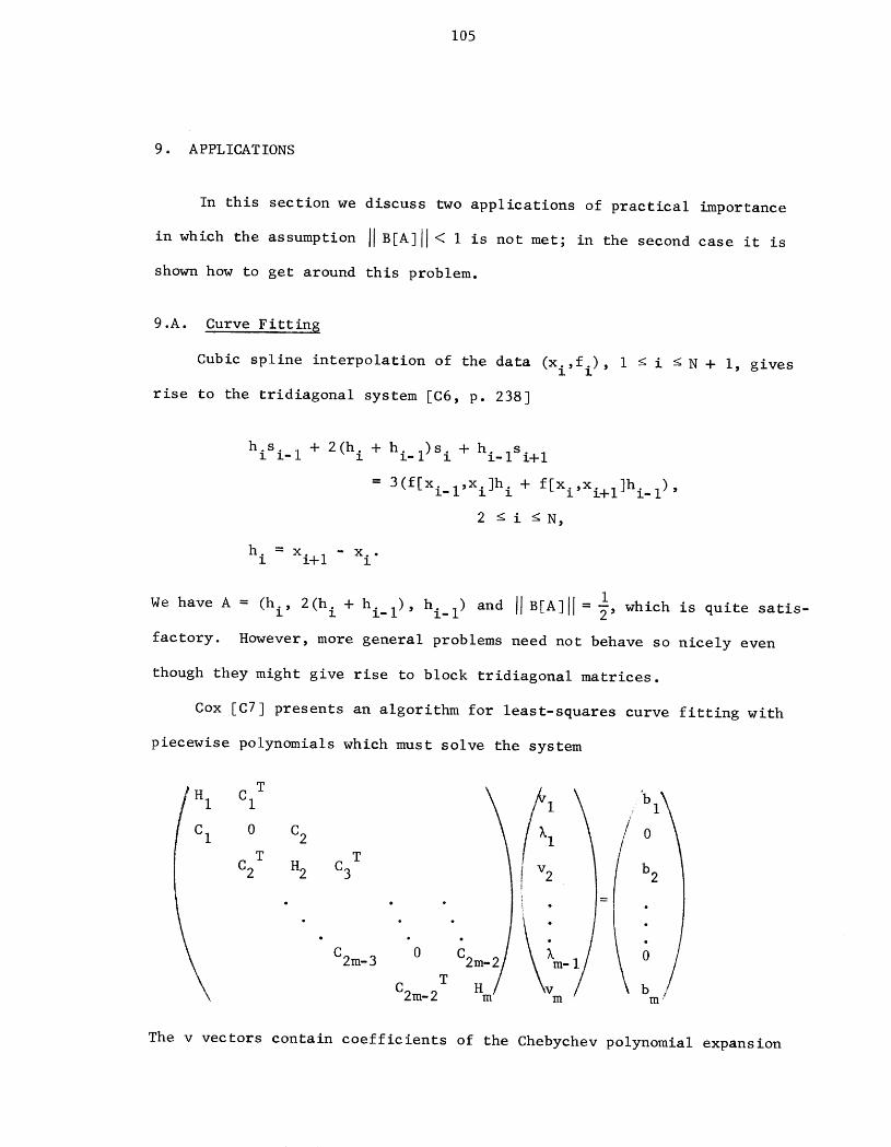
105

9 • APPLICATIONS

In this section we discuss two applications of practical importance

in which the assumption IIB[A]II < I is not met; in the second case it is

shown how to get around this problem•

9.A. Curve Fitt ins

Cubic spline interpolation of the data (xi,f i) , I _ i < N + i, gives

rise to the tridiagonal system [C6, p. 238]

hisi_ 1 + 2(h i + hi_l)S i + hi_isi+ I

= 3(f[xi_l,Xi]hi + f[xi,xi+l]hi_l),

2 _i _N,

----"X - X..hi i+l l

We have A = (hi, 2(h i + hi_l), hi_ 1) and IIB[A]I[ = 2' which is quite satis-

factory. However, more general problems need not behave so nicely even

though they might give rise to block tridiagonal matrices.

Cox [C7] presents an algorithm for least-squares curve fitting with

piecewise polynomials which must solve the system

HI CIT 1 1\

0 C2 I /

i. vb 2

•. "". !0 C2T

C2m- 2 m m"

The v vectors contain coefficients of the Chebychev polynomial expansion

106

of the piecewise polynomial, and the _ vectors contain Lagrange multipli-

ers derived through a constrained linear least-squares problem. The C o'S]

always have full rank, and if there are sufficiently many data points

between adjacent pairs of knots then the H o'S will all be positive defi-]

nite. In this case a straightforward band elimination may be used well

when the number of knots and data points is large. When insufficient data

is available the H.'s will not have full rank and pivoting is needed in]

the band elimination. It seems that the condition IIB[A]II < I will not

hold for any reasonable partitioning or data. Indeed, B[A] is not even .

defined for the most obvious partition.

9.B. Finite Elements

In Section 2.A we noted that matrices constructed from finite element

approximations to differential equations often do not satisfy assumptions

such as IIB[A]II < I. Thus some other technique must be used to establish

numerical stability in a direct method or convergence in an iterative

method. Usually it is shown that A is positive definite. The following

example, admittedly a simple one, shows how an easily implemented change

of variables can yield a new system A'x' = v' such that IIB[A' ]II< I.

Even if the change of variables is not actually made, this will show that

IIB[A]IIc_< i for some norm II" llc_,and also serves to establish numerical

stability.

Let us begin with the equation -u" = I on the unit interval. Using

Hermite cubics, Strang and Fix [$4, p. 59] derive the 4th order accurate

finite element equations

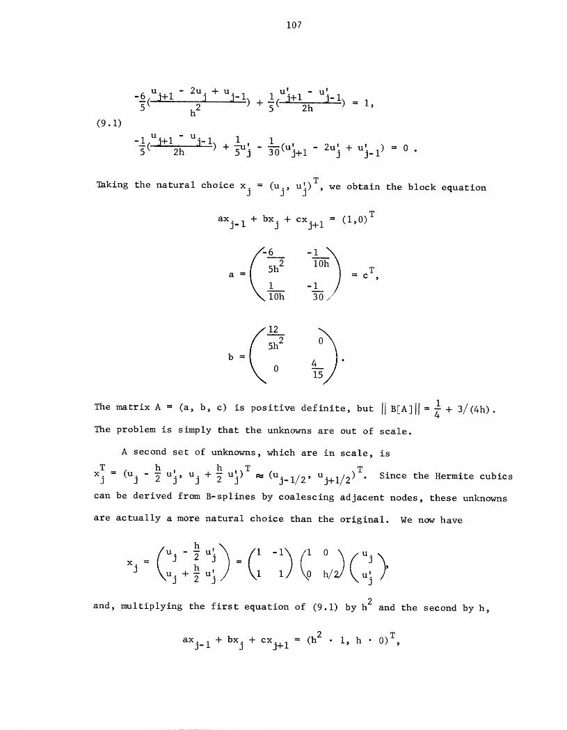
107

u - 2u + u u' - u'.

-6( j+l h2j j-I) +_I( J+12h J'l) = I,

(9.1)

u. - Uj_l) (uJ+ I- ( ]+I I I

2h + _-u'5j ---30 ' - 2u'j+ u'j_l) = 0 .

Taking the natural choice x. = T(uj u_) , we obtain the block equation] ' ]

T

axj_ I + bxj + cxj+ I = (I,0)

h2 T0h Ta: =c ,

b = •

I

The matrix A : (a, b, c) is positive definite, but IIB[A]II : _ + 3/(4h).

The problem is simply that the unknowns are out of scale.

A second set of unknowns, which are in scale, is

T (uj h h u_ T (uj_x. : - ' + ) _ 1/2 uj+I/2 )T] _ uj, uj _ ] , . Since the Hermite cubics

can be derived from B-splines by coalescing adjacent nodes, these unknowns

are actually a more natural choice than the original• We now have

] uj+_ J ]

and, multiplying the first equation of (9.1) by h2 and the second by h,

= (h2axj i + bxj + cxj+ I • I, h • 0)T

108

a : _ /6 1/30/,

1(12/5 12/5_

(9.2) = _k-8/15 8/5 J,

I ,""'7/5 -16_7 __ I/30 -I/ "

The blocks are independent of h and we have IIBEA]II : I, with Pk(B[A]) < I

for the first and last block rows. (Actually, this assumes Dirichlet

boundary conditions; Neumann conditions give Pk(B[A]) = i.)

For the more general equation -u" + Qu = f, Q a constant, the follow-

ing equations are derived [S4, p. 59]:

i

30---h(-36 uj_ I - 3h u'j_l + 72 uj - 36 Uj+l + 3h u'j+l)

+ Qh (54 u + 13 h u' + 312 u + 54 u - 13h '420 j- I j-I j j+l Uj+l)

--" F °_J

I -h u' + 8h u' - 3 u -h '_(3 uj_ I j-I j j+l Uj+l)

+ Qh2(-13 u - 3h u' + 8h u' + 13 u - 3 h '420 j-I J-I j j+l Uj+l)

_---FI .

J

T h hu,o TAgain taking X o = (u - u' u + ) and suitably scaling the equa-3 J _ J' j _ J

tions, they become

T

dEj_ I + bxj + cxj+ I = (hFj,Fj)

where now the blocks are O(h 2) perturbations of the blocks in (9.2). Omit-

5

ting details, for h sufficiently small this gives IIB[A]II = I - _ Qh 2 + O(h4).

109

Since rescaling and change of variables in the linear system is equiv-

alent to a change of basis in the original function subspace, the process

should be applicable to more general differential equations solved by

finite element methods. The underlying technique is to prove something

for spline approximations, and show that the property carries over in the

collapse of nodal points yielding the Hermite cubic approximations.

Strictly in terms of modifying linear systems by a block diagonal

scaling, it is natural to ask if either of the following problems are

solvable in general:

I. Given an arbitrary block tridiagonal matrix A, find a block

diagonal matrix E such that IIB[AE]II < I.

2. In I., if IIB[A]II < I, find E such that IIB[AE]II < IIB[A]II.

These problems are closely related to the optimal diagonal scaling of

matrices to minimize condition numbers, and as such are outside the scope

of this thesis.

110

I0. IMPLEMENTAT ION OF ALGOR IT_IMS

This section contains some general remarks on the choice of algorithm

for particular applications, and a more detailed comparison of algorithms

for use on a vector computer. In the comparison we assume uniform nXn

block sizes, later specialized to n = 2. All algorithms will use the same

data layout, assumed to be core-contained, and the execution time compari-

son will be in two parts: first for a very simplified and idealized model

in which the machine vectors are defined as storage locations in arithmetic

progression, and second for a model in which the machine vectors are defined

as contiguous storage locations (arithmetic progression with increment = I).

The first model uses information for the CDC STAR-100 ignoring, among other

things, the fact that machine vectors on STAR must satisfy the conditions

for the second model. This double comparison allows us to pinpoint the

effect of data manipulation required by the stringent requirement on vec-

tor operands. For a description of STAR facilities necessary for this dis-

cussion, see Section 2.B and Appendix A. Implementation of algorithms for

tridiagonal linear systems, n = I, is adeq_aately discussed elsewhere ([H4],

[Jl], [L2], [MI], [$2]) and these references may be considered as back-

ground material for this section.

10.A. Choice of Algorithm (Generalities)

The salient point of our analysis has been that a number of algorithms

may be applied to block tridiagonal linear systems that are likely to arise

in practice. Sometimes it may be possible to take advantage of special

features in order to reduce computing costs or estimate error. When the

computing costs are high (such as one enormous problem or a large problem

solved repeatedly) an extra effort must be made to choose the most

III

efficient algorithm. This choice will be difficult to make in general,

but we feel that it is not at all difficult to choose good algorithms

in many cases.

Regardless of the computer involved, algorithms for three special

problems should be implemented before proceeding to algorithms for more

general problems. The first should deal with general block tridiagonal

matrices restricted to blocks of a small uniform size, say no more than

8×8. On a standard sequential computer, band or profile methods are ap-

propriate; on a k-parallel computer some form of block LU factorization

should be used, and on a vector computer a combination of odd-even reduc-

tion and LU factorization should be used. Storage allocation and access,

vector operations on a parallel or vector computer and implementation

issues in general can be greatly simplified under the block size restric-

tion. Options include implementation as a set of subroutines for specific

block sizes, insertion of tests for use as a semidirect method, and spe-

cial scalings or pivoting strategies for efficiency or stability. This

restricted class of algorithms may be applied directly to small-block

problems or used as a module in the iterative solution of large sparse

problems as indicated in Section 8. The experience gained may or may not

be useful for implementation of methods for moderate-sized blocks, which,

in our opinion, should be treated in a different manner.

The best choice of a parallel algorithm for moderate-sized blocks is

not clear at this time. These cases represent a cross-over between effi-

cient vector implementations of band/profile methods and the odd-even

methods. Either one is likely to be satisfactory. In Lambiotte's opinion

ILl] the band methods are better for the CDC STAR, but this choice is

heavily influenced by vector addressing restrictions on the STAR (cf. our

112

remarks in Section 10.B). Other parallel or vector computers may not

present such problems, and a more complete analysis is needed.

The third basic class of algorithms are the fast Poisson solvers,

including generalizations. Recent studies have shown that many finite dif-

ference approximations to elliptic equations can be computed very effi-

ciently by iterative or modification methods based on the Poisson solvers.

There are several kinds of algorithms to choose from, and all have consid-

erable inherent parallelism. Other algorithms are available for elliptic

eqoations, but flexibility and ease of implementation suggest that Poisson-

based algorithms should be among the first to be considered. Brandt's

multi-level adaptive methods [BI3] must also be seriously considered.

Finally, we note that matrix partitioning and block elimination is a

useful technique for dealing with matrices so large that secondary storage

must be used [R4]. Known as the hypermatrix scheme in other contexts, it

has been extensively exploited by theASKA system, a structural analysis

package developed at the University of Stuttgart IF3]. Noor and Voigt IN1]

discuss implementation of hypermatrix schemes on the CDC STAR-100. l_e

method works as follows: suppose a partition TT is given (see Section 2.A),

and let A be the matrix A partitioned accordingly. Block sizes in ASKATT

are chosen to optimize transfers between storage levels, while the choice

on STAR must also try to maximize vector lengths and hence minimize start-

up costs. The usual situation is that a few blocks of A will be in main

memory, while the bulk of A will be in secondary memory. For example, ifTT

_' is another partition such that _ refines _', we would perform block

elimination on ATT,XTT, = VTT,. When A is block tridiagonal so is ATT,TT

Since the data requirements for the LU or Cholesky factorization are then

highly localized, this is a natural procedure [E3]. Moreover, the diagonal

113

blocks of Am, will themselves be block tridiagonal, though possibly of low

order. As noted in Sections 2.A and 3.A.2, if IIB[A_]II < I then IIB[A, ]II

< IIBIAs]If, and pivoting will be restricted to those blocks of An, resi-

dent in main memory. This, of course, is precisely what is desired.

10.B. Storage Requirements

Data layout is an essential part of planning an algorithm's imple-

mentation on any parallel computer, since computational speed can be

severely decreased if data cannot be accessed conveniently. On a vector

computer this means that conceptual vectors must conform to the machine's

definition of a vector operand. We consider some consequences of this

requirement for implementation on the CDC STAR-100, assuming that the prob-

lem is core-contained.

Storage available on the STAR, for 64-bit words, consists of 256 reg-

isters and either 512K or IM words of main memory. A sizable secondary

disc storage is also available but will not be considered here. A vector

on STAR consists of s consecutive storage locations, I _ s < 64K.

Our data arrangement for block tridiagonal linear systems with uniform

n×n blocks is illustrated in fig. i0. i for the case n = 2, N = 7. Define

m = Flog2N], N* = 2m, and if N < N* then extend Ax = v with N* - N trivial

equations x. = 0. The matrix A and vector v can then be held in threel

storage vectors of length n2N * and one of length nN*. Taking the subdiag-

2

onal blocks as an example, the n components of ak are aij,k , I < i -_n,

I < j < n, I _ k _ N*, and the storage vector a is defined by

Thus a total of (3n2 + n)N* loca-a((i - l)N*n + (j - I)N* + k) = aij,k.

tions are needed to store the original system. We do not consider the

cost of setting up the storage vectors since each of our algorithms will

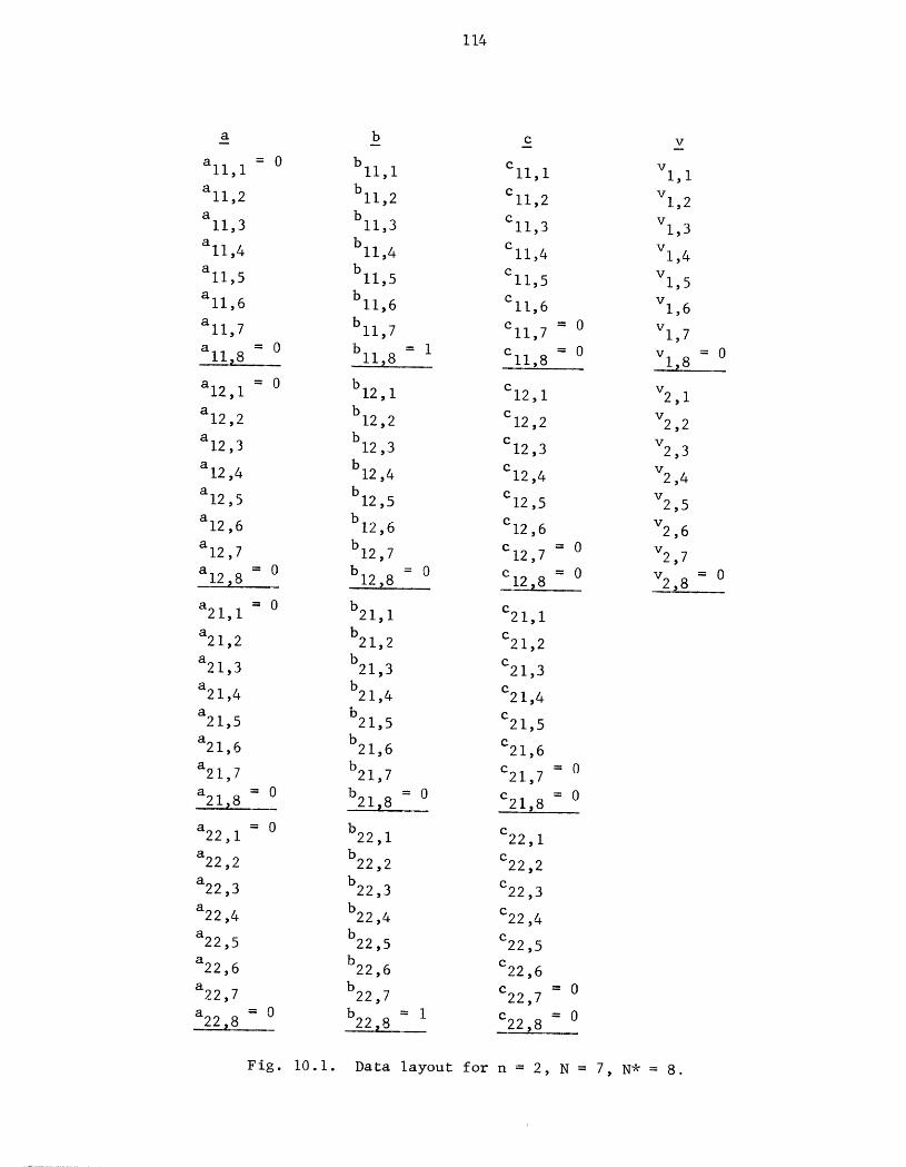
c _I,I

b c ii ,k

a b 3.1 ,I c II ,Z _ k,3

" = 0 bll,Z cll'3

b ,L_ cli'5 _%.,6

eL%I,L_ bll,5 cI_"6 _. 0 ,jl_.... "

S.ll,5 bll,6 cll''/ =. 0 I"b %..I,q c%_._.-._ v,2.,I

ai%,6 _ % v ,2b i_ c12,% Z

all,7 = 0 -I v ,3

_IZ ,k b 12,2 c 12,3 _Z ,a

a12,2 b _% ,3 cl, z ,a v Z,5",r2,6

a12,3 bl2'a cll'5 _2'7 _ 0

s.%.Z,6 blz'7 _ 0

b I?..._ c,ZI,I_'I2"'7 -_..0

a%__ 0 bll,l c?-1,2

a21, _ = b2.1,2 c'2.1'3b 2.%,3 c 2.%.,5

a?.l,Z bzl'_ c7_1,5alk,3 c21 6

bz%5 ' ._{3aZ%,a

all'5 bzl,6 c11'7 _ O

_.Z%..,6 b21,7 _ C) c_%.._bl_ clz ,l

aZl,7 ¢. O "I c ,l

= c12. ,3all ,I bzl ,l

alZ ,l bl1,3 cll '_"

a22,3 bzz ,L_ cz1,5

_'12, a bzz,5 c2z'6 -_. 0b22,6 cll,7 _.0

a,2.2 ,5 cZl_ _,.

aZl,7 b ll_% _ _ Z, _ _ 7,

Data layout £o_ 9-lO .I.

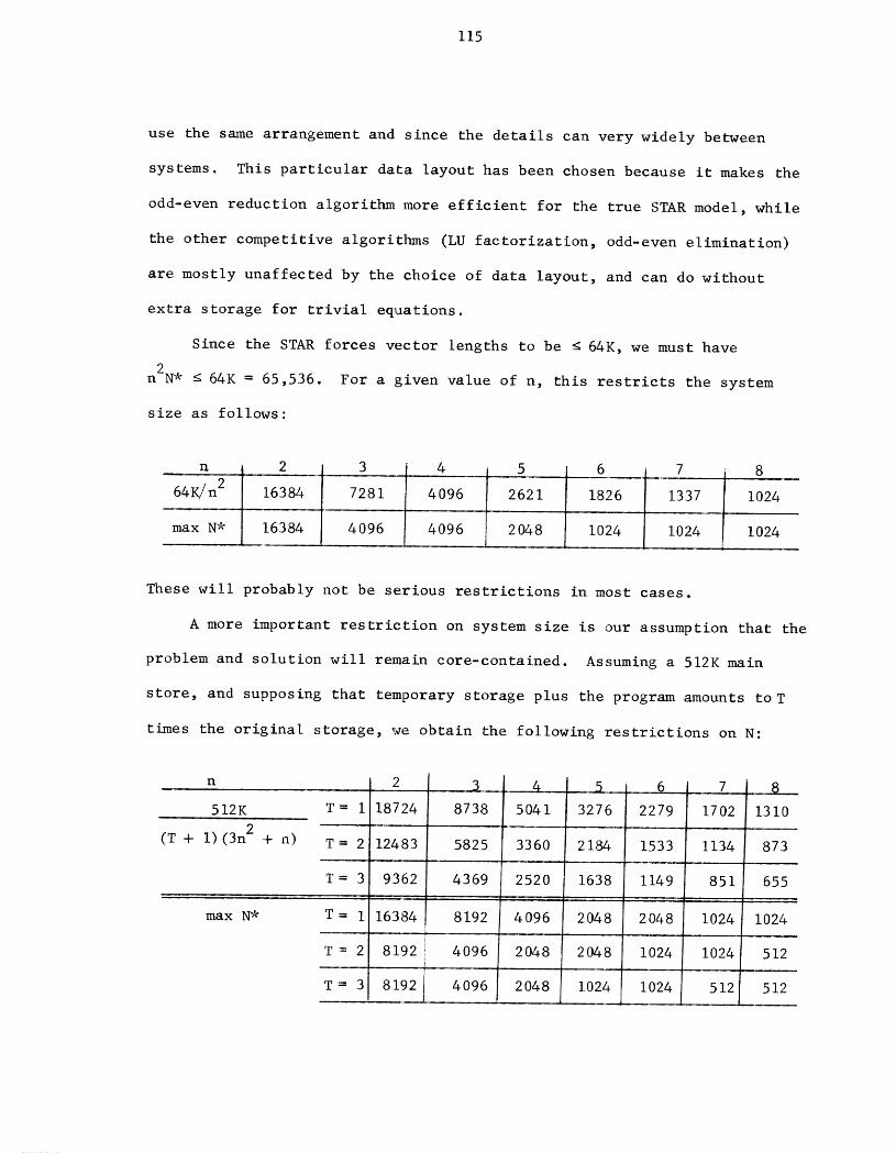
115

use the same arrangement and since the details can very widely between

systems. This particular data layout has been chosen because it makes the

odd-even reduction algorithm more efficient for the true STAR model, while

the other competitive algorithms (LU factorization, odd-even elimination)

are mostly unaffected by the choice of data layout, and can do without

extra storage for trivial equations.

Since the STAR forces vector lengths to be _ 64K, we must have

2

n N* < 64K = 65,536. For a given value of n, this restricts the system

size as follows:

n 2 3 4 5 6 7 8±---- I

64K/n 2 [6384 7281 4096 2621 1826 1337 1024

max N* [6384 4096 4096 2048 1024 1024 1024,

These will probably not be serious restrictions in most cases.

A more important restriction on system size is our assumption that the

problem and solution will remain core-contained. Assuming a 512K main

store, and supposing that temporary storage plus the program amounts to T

times the original storage, we obtain the following restrictions on N:

n 2 ....$__.. 4 5 6 7 $

512K T: 1 18724 8738 5041 3276 2279 1702 1310

(3n2(T + I) + n) T: 2 12483 5825 3360 2184 1533 1134 873

...._ :

T = 3 9362 4369 2520 1638 1149 851 655

max N* T= 1 16384 8192 4096 2048 2048 1024 1024

T = 2 8192! 4096 2048 2048 1024 1024 512

T = 3 8192 I 4096 2048 1024 1024 512 512L

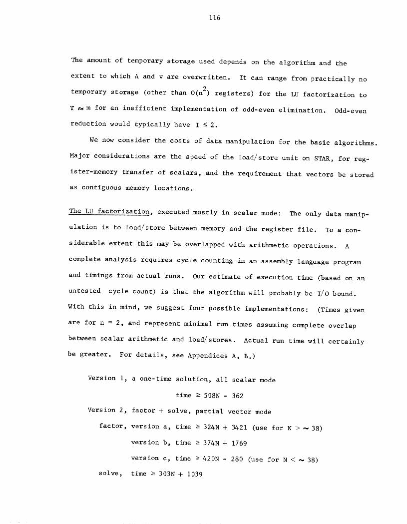
116

The amount of temporary storage used depends on the algorithm and the

extent to which A and v are overwritten. It can range from practically no

temporary storage (other than O(n 2) registers) for the LU factorization to

T _ m for an inefficient implementation of odd-even elimination. Odd-even

reduction would typically have T _ 2.

We now consider the costs of data manipulation for the basic algorithms.

Major considerations are the speed of the load/store unit on STAR, for reg-

ister-memory transfer of scalars, and the requirement that vectors be stored

as contiguous memory locations.

The LU factorization, executed mostly in scalar mode: The only data manip-

ulation is to load/store between memory and the register file. To a con-

siderable extent this may be overlapped with arithmetic operations. A

complete analysis requires cycle counting in an assembly language program

and timings from actual runs. Our estimate of execution time (based on an

untested cycle count) is that the algorithm will probably be I/0 bound.

With this in mind, we suggest four possible implementations: (Times given

are for n = 2, and represent minimal run times assuming complete overlap

between scalar arithmetic and load/stores. Actual run time will certainly

be greater. For details, see Appendices A, B.)

Version I, a one-time solution, all scalar mode

time > 508N - 362

Version 2, factor + solve, partial vector mode

factor, version a, time > 324N + 3421 (use for N > _ 38)

version b, time >-374N + 1769

version c, time _ 420N - 280 (use for N < -_ 38)

solve, time e 303N + 1039

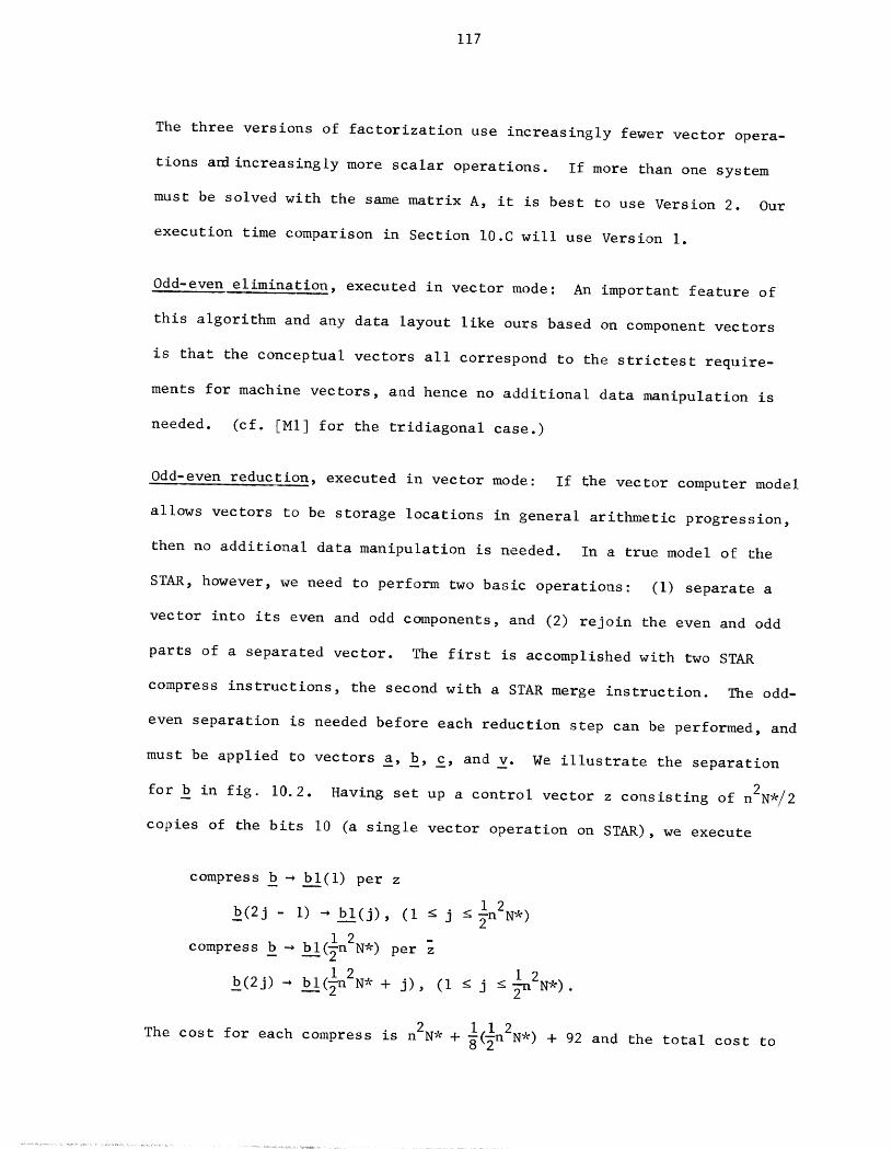
117

The three versions of factorization use increasingly fewer vector opera-

tions and increasingly more scalar operations. If more than one system

must be solved with the same matrix A, it is best to use Version 2. Our

execution time comparison in Section 10.C will use Version I.

Odd-even elimination, executed in vector mode: An important feature of

this algorithm and any data layout like ours based on component vectors

is that the conceptual vectors all correspond to the strictest require-

ments for machine vectors, and hence no additional data manipulation is

needed. (cf. [MI] for the tridiagonal case.)

Odd-even reduction, executed in vector mode: If the vector computer model

allows vectors to be storage locations in general arithmetic progression,

then no additional data manipulation is needed. In a true model of the

STAR, however, we need to perform two basic operations: (I) separate a

vector into its even and odd components, and (2) rejoin the even and odd

parts of a separated vector. The first is accomplished with two STAR

compress instructions, the second with a STAR merge instruction. The odd-

even separation is needed before each reduction step can be performed, and

must be applied to vectors a, _b, _c, and _v" We illustrate the separation

for b in fig. 10.2. Having set up a control vector z consisting of n2N*/2

copies of the bits I0 (a single vector operation on STAR), we execute

compress b _ b__l(1)per z

12

b(2j - I) _ bl(j), (I < j _n N*)

compress b _ bl(2n2N*)--perz

1 2 , 1 2.,_b(2j) _ b!l(_n N_ + j), (I K j _n i_j.

I.I 2 ..The cost for each compress is n2N * + _(_n N_) + 92 and the total cost to

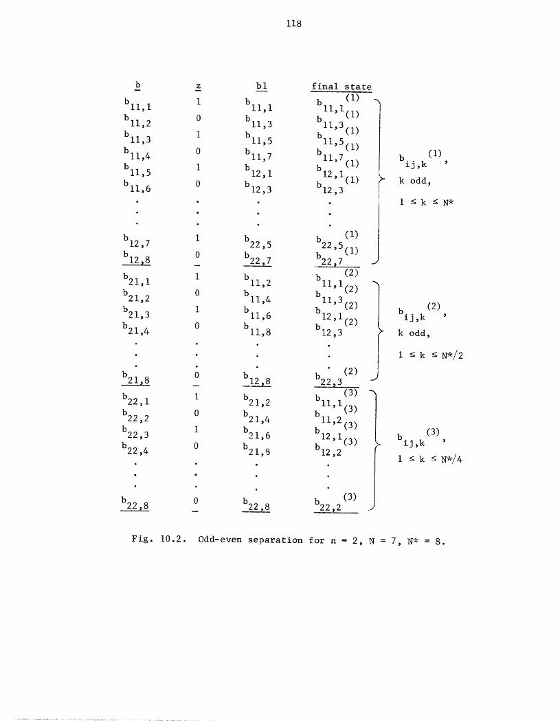
118

b z bl final state

bll,l I bll,l bll,l (I)

bll,2 0 bll,3 bll,3 (I)(1)

bll,3 I bll,5 bll,5(l )(1)

bll,4 0 bll,7 bll'7 (I) bij,k '

bll,5 1 b12,1 b12' 1(1) _" k odd,bll,6 0 bi2,3 b12,3

.... I _k <N*

(1)

b12,7 1 b22,5 b22,5(1)

b12,8 _0 b2_2 7 b22_7 J(2)

b21,1 1 bll,2 bll ' 1(2)

b21,2 0 bll,4 b11'3(2) bij, k(2) ,b21,3 1 b11,6 b12,1(2 )b21,4 0 bi1,8 bi2,3 k odd,

.... i _ k _ N*/2

b21_ 8 _ (2)0 b22_3, , , _

b22,1 i b21,2 bll,l (3) -_

b22,2 0 b21,4 bll, 2 (3)

(3) (3)

b22,3 I b21,6 b12' I(3) bij k 'b22,4 0 b21,8 b12,2 _ '

1 < k _ N*/4

b22_8 0 b22 8 b22 2(3)

Fig. 10.2. Odd-even separation for n = 2, N = 7, N* = 8.

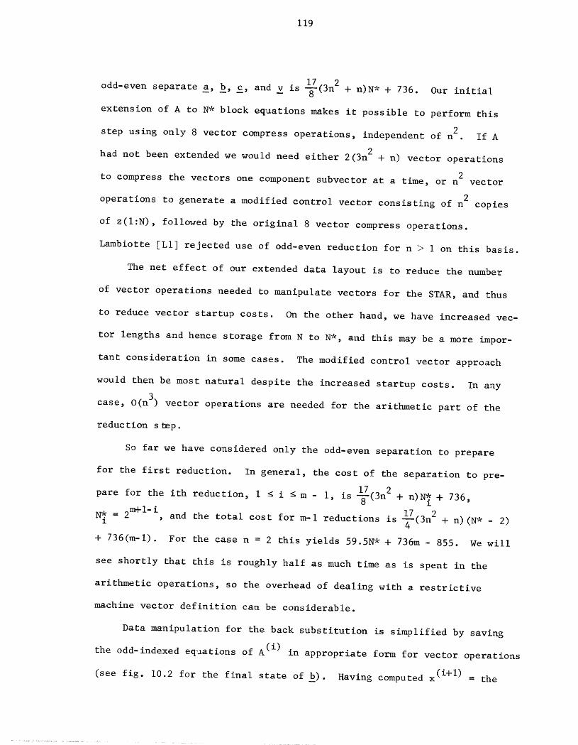
I19

separate a, _b, _c, and _v is 17_(3n2 + n)N* + 736. Our initialodd-even

extension of A to N* block equations makes it possible to perform this

2step using only 8 vector compress operations, independent of n . If A

had not been extended we would need either 2 (3n2 + n) vector operations

2to compress the vectors one component subvector at a time, or n vector

2operations to generate a modified control vector consisting of n copies

of z(l:N), followed by the original 8 vector compress operations.

Lambiotte ILl] rejected use of odd-even reduction for n > I on this basis.

The net effect of our extended data layout is to reduce the number

of vector operations needed to manipulate vectors for the STAR, and thus

to reduce vector startup costs. On the other hand, we have increased vec-

tor lengths and hence storage from N to N*, and this may be a more impor-

tant consideration in some cases. The modified control vector approach

would then be most natural despite the increased startup costs. In any

case, O(n 3) vector operations are needed for the arithmetic part of the

reduction step.

So far we have considered only the odd-even separation to prepare

for the first reduction. In general, the cost of the separation to pre-

17 (3n2pare for the ith reduction, I < i < m- I is -_ + n)N* + 736,

17 "

N*l = 2m+l-i' and the total cost for m-I reductions is _-(3n 2 + n)(N* - 2)

+ 736(m-I). For the case n = 2 this yields 59.5N* + 736m - 855. We will

see shortly that this is roughly half as much time as is spent in the

arithmetic operations, so the overhead of dealing with a restrictive

machine vector definition can be considerable.

Data manipulation for the back substitution is simplified by saving

the odd-indexed equations of A (i) in appropriate form for vector operations

(see fig. 10.2 for the final state of b). Having computed x (i+l) = the

120

even components of x(i) , we compute the odd components of x (i) and merge

the two sets into x (i). The merge operation on STAR is comparatively

more expensive than the compress operation, but we are only dealing with

the solution vector and not blocks of A. The cost of the merge operation

at stage i is 3nN.* + 123, and the total cost for m-I reductions isI

6n(N* - 2) + 123(m - i). For n = 2 this yields 12N* + 123m - 147.

p-fold reduction: Suitable data arrangement and use of control vectors

for p-fold reduction can readily be generalized from our discussion of

odd-even reduction. The odd-even separation generalizes to separation

into p vectors, which requires p compress instructions per storage vector;

the cost per reduction would be (p + l)(3n 2 + n)N * + 368p, N * = pm+l-ii i '

m = rlOgpN_. The back substitution requires merging p vectors into l,

using p-I merge instructions at cost of 3(_-- - l)nN*+ 123(p-I) to goP i

(i+l) (i)from x to x ° It is clear that these costs are minimized by

p=2.

Jacobi iterations: Data manipulation is unnecessary when A and v or B[A]

-iand DIAl v are stored according to our component subvector scheme.

10.C. Comparative Timing Analysis.

we close with an execution time comparison of algorithms for general

block tridiagonal systems with 2×2 blocks, based on timing information for

the CDC STAR-100. This will expand the crude comparison of the LU factor-

ization and odd-even reduction given in Section 4.D, and illustrates many

earlier statements concerning the cost of various methods. Essential con-

siderations include vector startup costs, creating a substantial penalty

for operations on short vectors, and data manipulation to deal with

121

restrictive definitions of vector operands. Section 10.B began our dis-

cussion of the latter problem.

Our initial simplified analysis is based on the following conven-

tions, which allow us to consider only arithmetic costs:

I. we assume

a. vector operands may be any sequence of storage locations

in arithmetic progression,

b. pivoting is never necessary;

2. we ignore

a. instruction overlap capabilities,

b. address calculations, loop control and termination tests,

c. load/store costs for scalar operands,

d. storage management costs, as a consequence of assumption l.a.

Our second, and more realistic analysis will demand that vector operands

consist of consecutive storage locations, so we must consider storage manage-

ment as explained in Section 10.B. Overlap, loop control and scalar load/

store will also be considered, but not address calculation or termination

of iterations. Algorithms and timing derivations are given in Appendix B;

here we present the main results and make comparisons.

Execution times for the basic direct methods are initially estimated

as follows (m = Flog2N]):

I. the block LU factorization, using scalar operations only (LU):

1012N- 784

2. odd-even elimination, using vector operations only (OEE):

94.5Nm + 12999m - 93.5N - 1901

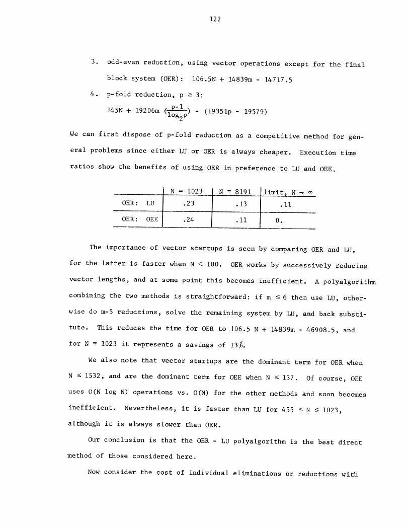
122

3. odd-even reduction, using vector operations except for the final

block system (OER): I06.5N + 14839m- 14717.5

4. p-fold reduction, p e 3:

145N + 19206m(log2p) - (19351p- 19579)

We can first dispose of p-fold reduction as a competitive method for gen-

eral problems since either LU or OER is always cheaper. Execution time

ratios show the benefits of using OER in preference to LU and OEE.

N = 1023 N......= 8191 l_it_ N _

OER: LU .23 .13 .II

OER: OEE .24 .II 0.

The importance of vector startups is seen by comparing OER and LU,

for the latter is faster when N < I00. OER works by successively reducing

vector lengths, and at some point this becomes inefficient. A polyalgorithm

combining the two methods is straightforward: if m _ 6 then use LU, other-

wise do m-5 reductions, solve the remaining system by LU, and back substi-

tute. This reduces the time for OER to 106.5 N + 14839m - 46908.5, and

for N = 1023 it represents a savings of 13_.

We also note that vector startups are the dominant te_n for OER when

N _ 1532, and are the dominant term for OEE when N _ 137. Of course, OEE

uses O(N log N) operations vs. O(N) for the other methods and soon becomes

inefficient. Nevertheless, it is faster than LU for 455 _ N < 1023,

although it is always slower than OER.

Our conclusion is that the OER- LU polyalgorithm is the best direct

method of those considered here.

Now consider the cost of individual eliminations or reductions with

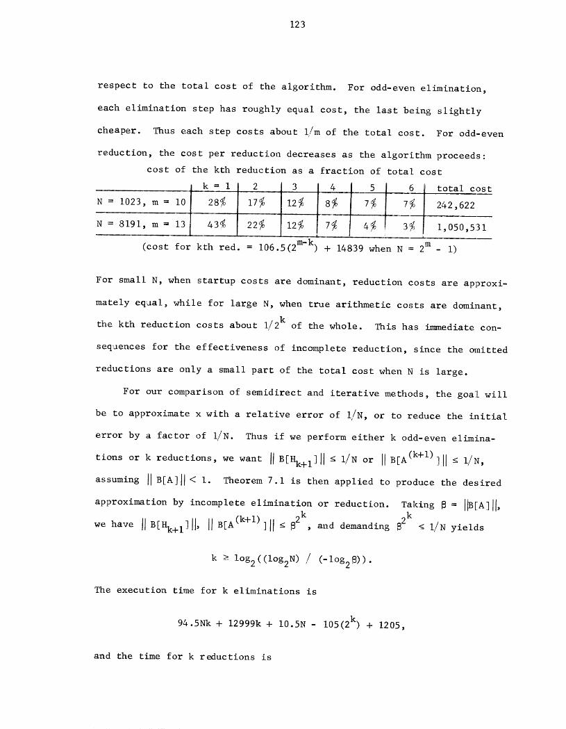
123

respect to the total cost of the algorithm. For odd-even elimination,

each elimination step has roughly equal cost, the last being slightly

cheaper. Thus each step costs about l,/mof the total cost. For odd-even

reduction, the cost per reduction decreases as the algorithm proceeds:

cost of the kth reduction as a fraction of total cost

N = 1023, m = I0 28_0 17¢ I 7¢ 242,622: , _

N 8191, m 13 434 22_ ] 12_ ! 7_ I 4_ ! 3_o 1,050,5:31i

(cost for kth red. = 106.5(2 m-k) + 14839 when N = 2m - i)

For small N, when startup costs are dominant, reduction costs are approxi-

mately equal, while for large N, when true arithmetic costs are dominant,

the kth reduction costs about i/2k of the whole. This has immediate con-

seqaences for the effectiveness of incomplete reduction, since the omitted

reductions are only a small part of the total cost when N is large.

For our comparison of semidirect and iterative methods, the goal will

be to approximate x with a relative error of l/N, or to reduce the initial

error by a factor of I/N. Thus if we perform either k odd-even elimina-

tions or k reductions, we want IIB[Hk+l]ll _ I/N or JlB[A(k+I)]II _ l/N,

assuming IIB[A]II < I. Theorem 7.1 is then applied to produce the desired

approximation by incomplete elimination or reduction. Taking 8 = I_[A]II,

we have IIB[Hk+ I]II, IiB[A(k+I) ]II _ 82k, and demanding 82k < I/N yields

k > log2((log2N ) / (-log 2B)).

The execution time for k eliminations is

94.5Nk + 12999k + 10.5N - I05(2k) + 1205,

and the time for k reductions is

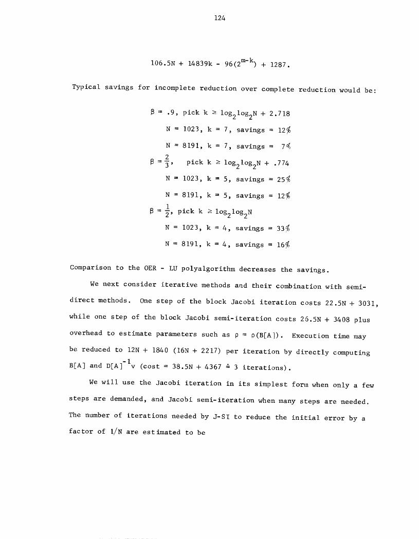
124

I06.5N + 14839k- 96(2m-k) + 1287.

Typical savings for incomplete reduction over complete reduction would be:

= .9, pick k >- log21og2N + 2.718

N = 1023, k = 7, savings = 12_

N = 8191, k = 7, savings = 7<

2

=_, pick k ->log21og2N + .774

N = 1023, k = 5, savings = 254

N = 8191, k = 5, savings = 12_

1

= _, pick k _ log21og2N

N = 1023, k = 4, savings = 33_

N = 8191, k = 4, savings = 16_

Comparison to the OER - LU polyalgorithm decreases the savings.

We next consider iterative methods and their combination with semi-

direct methods. One step of the block Jacobi iteration costs 22.5N + 3031,

while one step of the block Jacobi semi-iteration costs 26.5N + 3408 plus

overhead to estimate parameters such as p = p(B[A]). Execution time may

be reduced to 12N + 1840 (16N + 2217) per iteration by directly computing

B[A] and D[A]-Iv (cost = 38.5N + 4367 - 3 iterations).

We will use the Jacobi iteration in its simplest fo_n when only a few

steps are demanded, and Jacobi semi-iteration when many steps are needed.

The number of iterations needed by J-SI to reduce the initial error by a

factor of I/N are estimated to be

125

The LU factorization is always faster than OEE, and is faster than

OER for N < 312. Vector startup costs are dominant in OEE for N < 152,

and in OER for N _ 798. The OER-LU polyalgorithm should perform m-6 reduc-

tions, solve the remaining system by LU, and back substitute. The time is

183N + 16233m - 70677, yielding a 164 saving over OER for N = 1023 but only

a 3_ saving for N = 8191.

The execution time for odd-even elimination is allocated as follows:

N = 1023 N = 8191

arithmetic 96_ 96overhead 4_ 4

results 874 984vector startups 134 2_

Analysis of the total time for odd-even reduction shows the greater impor-

tance of overhead operations:

N = 1023 results startups

ar ithme tic 33_ 40_ 73_overhead 23< 4_ 27_

56_ 44_

N = 8191 results startups _

arithmetic 524 Ii_ 62__overhead 37_ I_ 38_

88_ 12_

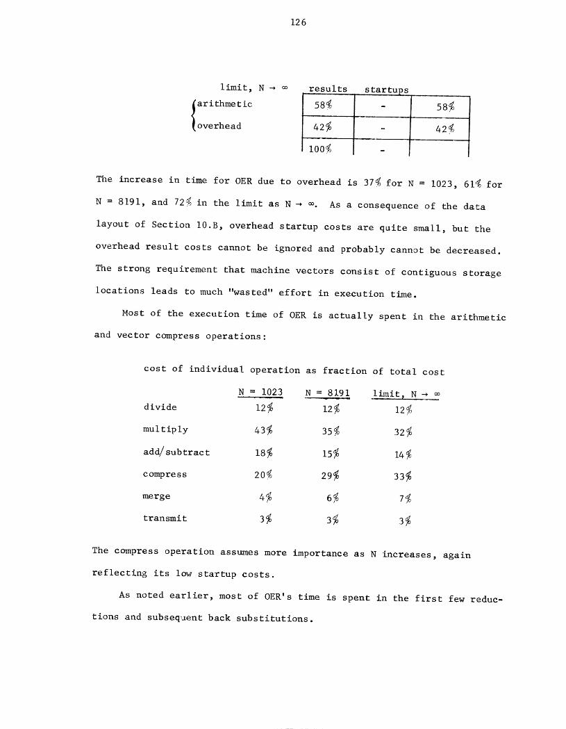
126

limit, N -_ _ results startups ........

arithmetic 58@o - 58__overhead 42_ - 42_

I00_

The increase in time for OER due to overhead is 37_ for N = 1023, 61_ for

N = 8191, and 724 in the limit as N-_ 0o. As a consequence of the data

layout of Section 10.B, overhead startup costs are quite small, but the

overhead result costs cannot be ignored and probably cannot be decreased.

The strong requirement that machine vectors consist of contiguous storage

locations leads to much "wasted" effort in execution time.

Most of the execution time of OER is actually spent in the arithmetic

and vector compress operations:

cost of individual operation as fraction of total cost

N = 1023 N = 8191 li_nit, N -_

divide 12_ 12_ 12_0

multiply 43_ 35_ 32_

add/subtract 18_ 15_ 14

compress 20_o 29_ 33_

merge 4_ 6_ 7

transmit 3_ 3_ 3_

The compress operation assumes more importance as N increases, again

reflecting its low startup costs.

As noted earlier, most of OER's time is spent in the first few reduc-

tions and subsequent back substitutions.

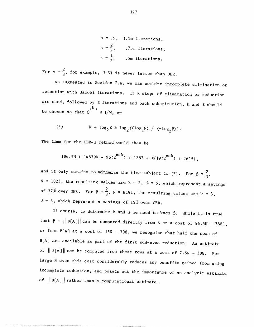
127

P = .9, 1.5m iterations,

2.75m iterations,p = --3'

I0 = --

2 ' .5m iterations.

2

For p = _, for example, J-SI is never faster than OER.

As suggested in Section 7.A, we can combine incomplete elimination or

reduction with Jacobi iterations. If k steps of elimination or reduction

are used, followed by _ iterations and back substitution, k and _ should

be chosen so that B2k_ < I/N, or

(*) k + iog2% >-log2((log2N) / (-log2B)).

The time for the OER-J method would then be

I06.5N + 14839k- 96(2m-k) + 1287 + _(19(2m-k) + 2615),

2

and it only remains to minimize the time subject to (*). For B = _,

N = 1023, the resulting values are k = 2, % = 5, which represent a savings

2

of 37°_ over OER. For _ = _, N = 8191, the resulting values are k = 3,

= 3, which represent a savings of 15_ over OER.

Of course, to determine k and _ we need to know _. While it is true

that _ = IIB[A][I can be computed directly from A at a cost of 46.5N + 3881,

or from B[A] at a cost of 15N + 308, we recognize that half the rows of

B[A] are available as part of the first odd-even reduction. An estimate

of IIB[A]II can be computed from these rows at a cost of 7.5N . 308. For

large N even this cost considerably reduces any benefits gained from using

incomplete reduction, and points out the importance of an analytic estimate

of IIB[A]II rather than a computational estimate.

128

This ends our initial comparison of algorithms. We now make the

assumption that vector operands are consecutive storage locations, allow

overlap of scalar operations, and consider the cost of loop control and

scalar load/store operations. The net effect is to lower the time esti-

mate for the LU factorization and raise the time estimate for odd-even

reduction. Odd-even elimination remains substantially unchanged. Rather

than simply recompute the figures presented earlier, which will be done in

a few cases, we try to indicate where the algorithms spend most of their

time.

Revised time estimates are given below. These should give a better

indication of actual runtime on STAR, but are probably all underestimates;

we note changes from the first set of timings, m = rlog2N].

i. LU factorization, (LU) 600N- 150

(a 40_ decrease due to use of instruction overlap)

2. Odd-even elimination, (OEE) 98.5Nm + 13403m - 101.5N - 2261

(a 4> increase due to overhead costs)

3. Odd-even reduction. (OER) 183N + 16233m - 16108

(a I0-70_ increase due to overhead costs; larger N incurs

larger increases).

Time ratios show the effect of decreasing the LU time and increasing the

OER time

N = 1023 N = 8191 limit, N -_ oo

OER :LU .54 .34 .31

OER :OEE .32 .17 0.

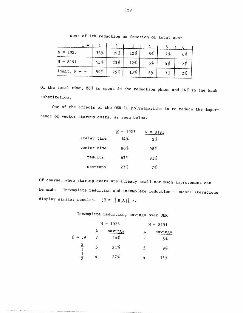
129

cost of ith reduction as fraction of total cost

i = 2 3 4 5 6

N = 1023 33_ 19_ 124 8_ 7_ 6_........ | J

N = 8191 45_ 23_ 12_ 6_ 4_ 2_

limit, N _ _ 5"0_ 25_ 13_ 6_ 3_ I--2_ -, .,

Of the total time, 86_ is spent in the reduction phase and 144 in the back

substitution.

One of the effects of the OER-LU polyalgorithm is to reduce the impor-

tance of vector startup costs, as seen below.

N = 1023 N = 8191

scalar time 14_ 2_

vector time 86_ 98_

results 634 91_

startups 23#0 7_0

Of course, when startup costs are already small not much improvement can

be made. Incomplete reduction and incomplete reduction + Jacobi iterations

display similar results. (8 = IIB[A]II )"

Incomplete reduction, savings over OER

N = 1023 N = 8191

k savings k savinss

8 = .9 7 I0_ 7 54

2 94o5 21_ 5

I

4 27_ 4 13_

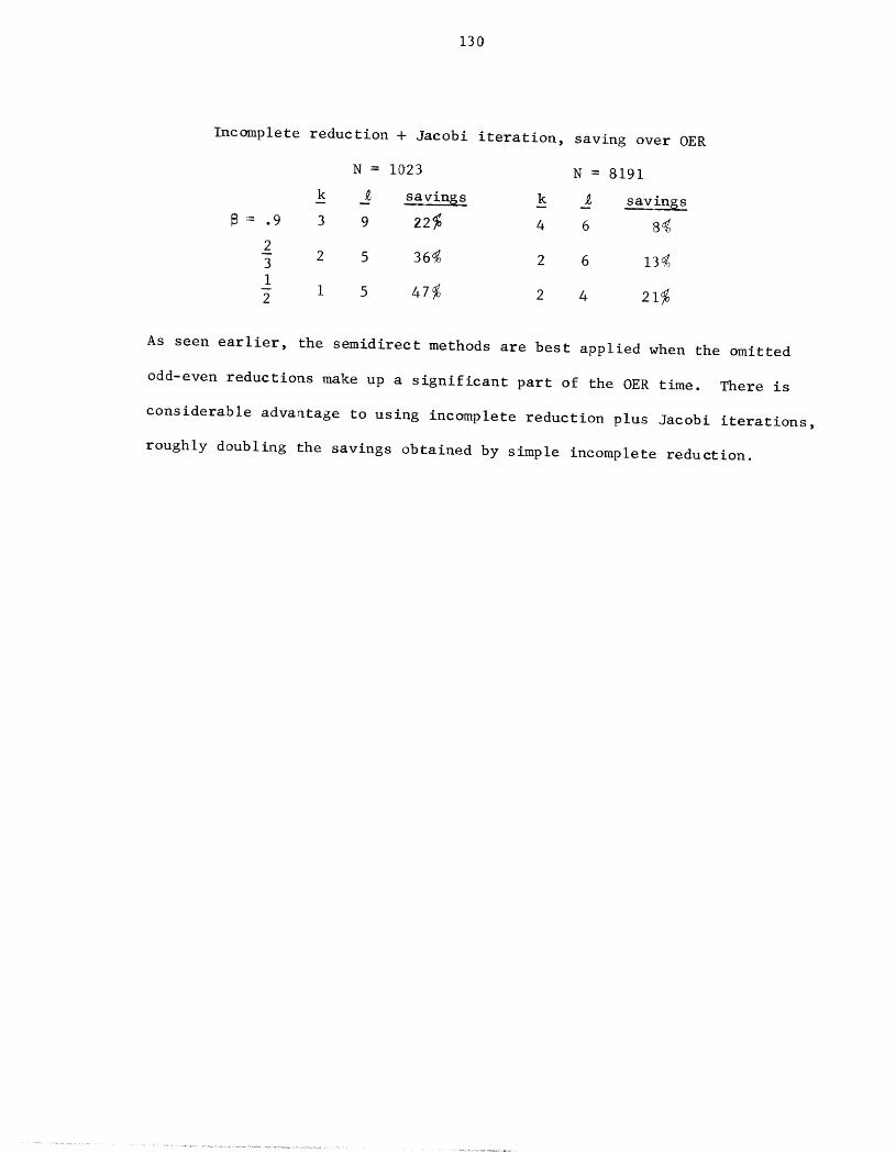
130

Incomplete reduction + Jacobi iteration, saving over OER

N- 1023 N = 8191

k 7 savings k __ sav_

= .9 3 9 22_ 4 6 8_o

2

2 5 364 2 6 13<i

I 5 47_ 2 4 21_2

As seen earlier, the semidirect methods are best applied when the omitted

odd-even reductions make up a significant part of the OER time. There is

considerable advantage to using incomplete reduction plus Jacobi iterations,

roughly doubling the savings obtained by simple incomplete reduction.

131

APPENDIX A

VECTOR COMPUTER INSTRUCTIONS

This section describes those features of the CDC STAR-100 needed for

our comparison of algorithms in Section I0. Information given here is

derived from CDC reference manuals and timing measurements made at Lawrence

Livermore Laboratory [C2], and by no means represents a complete discussion

of the STAR's facilities.

Execution times are for full-word (64 bit) floating point instructions,

given as the number of 40 nanosecond cycles needed for each instruction.

All times should be accurate to within 5_ except as noted, though actual

performance may be degraded somewhat due to memory conflicts.

A vector on STAR consists of N consecutive storage locations,

i < N < 65,536. The vect_length restriction is usually not serious, but

the need for consecutive storage is crucial. Other vector computers, the

TI ASC in particular, do not have this restriction. Both machines are

pipeline computers with the usual scalar instructions as well as vector

ins truc tions.

Useful features of vector instructions on STAR include:

broadcast constants - Most vector instructions allow a scalar (the broad-

cast constant, held in a register) to be transmitted repeatedly to form

one or both of the vector operands. Use of this facility decreases exe-

cution time in a few cases.

control vectors - Bit vectors can modify the effect of vector instructions,

such as suppressing storage to selected components of the result vector

or determining which operand components are to be used in an operation.

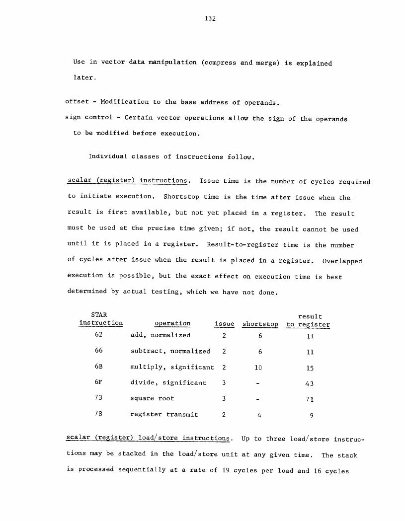
132

Use in vector data manipulation (compress and merge) is explained

later.

offset - Modification to the base address of operands.

sign control - Certain vector operations allow the sign of the operands

to be modified before execution.

Individual classes of instructions follow.

scalar (resister) instructions. Issue time is the number of cycles required

to initiate execution. Shortstop time is the time after issue when the

result is first available, but not yet placed in a register. The result

must be used at the precise time given; if not, the result cannot be used

until it is placed in a register. Result-to-register time is the number

of cycles after issue when the result is placed in a register. Overlapped

execution is possible, but the exact effect on execution time is best:

determined by actual testing, which we have not done.

STAR result

instruction o__peration issue shortstop to resister

62 add, normalized 2 6 II

66 subtract, normalized 2 6 II

6B multiply, significant 2 I0 15

6F divide, significant 3 - 43

73 square root 3 - 71

78 register transmit 2 4 9

scalar (register) load/store instructions. Up to three load/store instruc-

tions may be stacked in the load/store unit at any given time. The stack

is processed sequentially at a rate of 19 cycles per load and 16 cycles

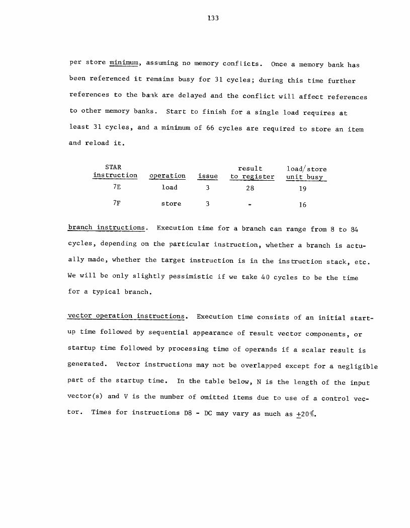
133

per store minimum, assuming no memory conflicts. Once a memory bank has

been referenced it remains busy for 31 cycles; during this time further

references to the ba_k are delayed and the conflict will affect references

to other memory banks. Start to finish for a single load requires at

least 31 cycles, and a minimum of 66 cycles are required to store an item

and reload it.

STAR result ioad/s tore

instruction operation issue to register unit bus__

7E load 3 28 19

7F store 3 - 16

branch instructions. Execution time for a branch can range from 8 to 84

cycles, depending on the particular instruction, whether a branch is actu-

ally made, whether the target instruction is in the instruction stack, etc.

We will be only slightly pessimistic if we take 40 cycles to be the time

for a typical branch.

vector operation instructions. Execution time consists of an initial start-

up time followed by sequential appearance of result vector components, or

startup time followed by processing time of operands if a scalar result is

generated. Vector instructions may not be overlapped except for a negligible

part of the startup time. In the table below, N is the length of the input

vector(s) and V is the number of omitted items due to use of a control vec-

tor. Times for instructions D8 - DC may vary as much as +204.

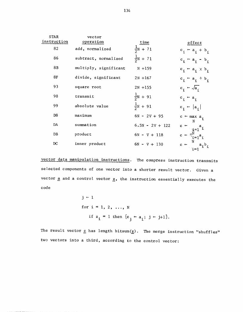
134

STAR vector

ins truc tion opera tion time effect

, normalized _N + 71 c. +- a. + b.82 addK. l l l

i

86 subtract, normalized _N + 71 c. +-a. -bl l i

8B multiply, significant N +159 c. +- a. × b.i i i

8F divide, significant 2N +167 c. +- a. + b.l i l

93 square root 2N +155 c. +-_.1 1

i98 transmit _N + 91 c. +- a.

l l

I

99 absolute value z_N + 91 c.I+- ''fail

D8 maximum 6N - 2V + 95 c +-max a.i

N

DA summation 6.5N- 2V + 122 c +- a.i-I l

N aDB product 6N - V + 118 c +- Hi= I i

NDC inner product 6N- V + 130 c +- a.bo

l l_i=I

vector data manipulation instructions. The compress instruction transmits

selected components of one vector into a shorter result vector. Giw_n a

vector _ and a control vector i, the instruction essentially executes the

code

j_l

for i = I, 2, ..., N

if z. = I then {c. +-a ; j +- j+l}I j i "

The result vector c has length bitsum_). The merge instruction "shuffles"

two vectors into a third, according to the control vector:

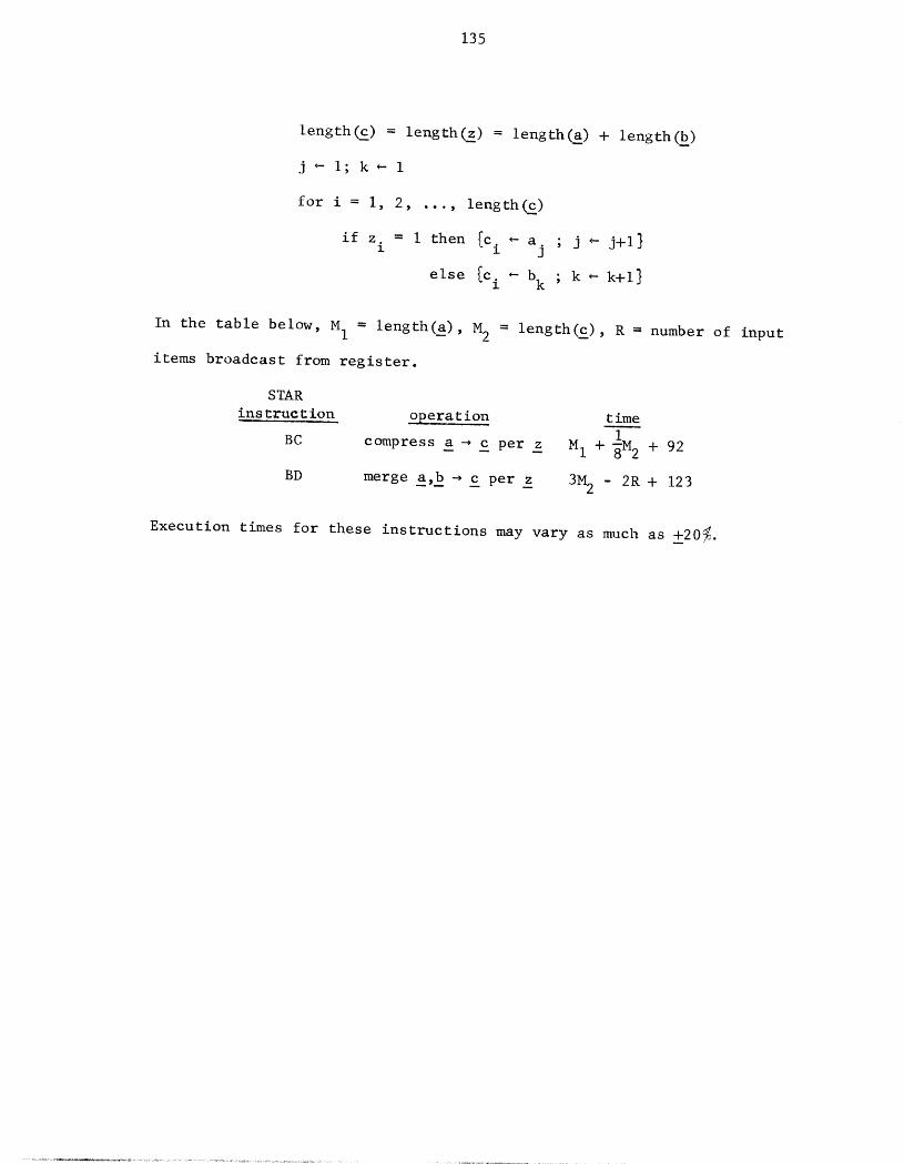
135

length(c) = length(z) = length(a) + length(b)

j_- i; k+-I

for i = I, 2, ..., length_)

if z. = I then [c. +- a ; j +- j+l}l l j

else _ci +- bk ; k _ k+l}

In the table below, MI -- lengthy), M2 = length(c), R = number of input

items broadcast from register.

STAR

ins t_uct ion opera tion timeI

BC compress a -_c per z M I + _M 2 + 92

BD merge a,b _ c per z 3M2 - 2R + 123

Execution times for these instructions may vary as much as +20_.

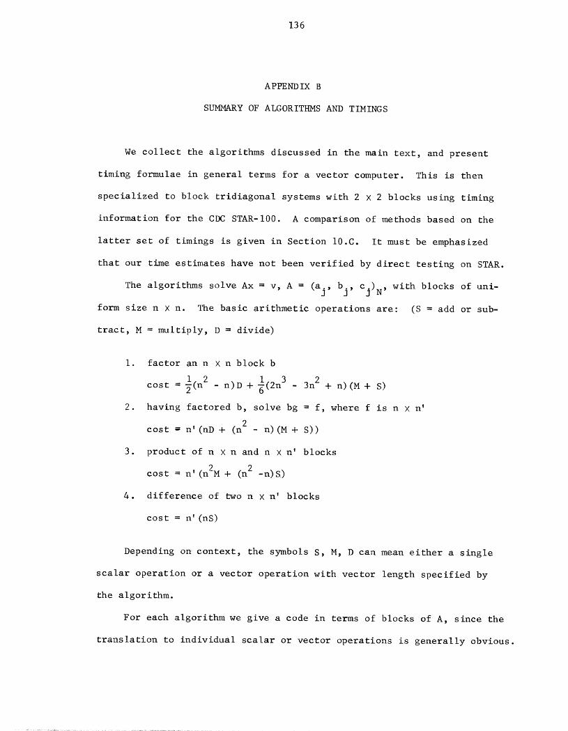
136

APPENDIX B

SUMMARY OF ALGORITHMS AND TIMINGS

We collect the algorithms discussed in the main text, and present

timing formulae in general terms for a vector computer. This is then

specialized to block tridiagonal systems with 2 × 2 blocks using timing

information for the CDC STAR-100. A comparison of methods based on the

latter set of timings is given in Section 10.C. It must be emphasized

that our time estimates have not been verified by direct testing on STAR.

The algorithms solve Ax = v, A = (aj, bj, Cj)N, with blocks of uni-

form size n × n. The basic arithmetic operations are: (S = add or sub-

tract, M = multiply, D = divide)

I. factor an n × n block b

i i 3

cost = _(n 2 - n)D + _(2n - 3n2 + n)(M + S)

2. having factored b, solve bg = f, where f is n × n'

cost _ n' (nD+ (n2 - n) (M + S))

3. product of n × n and n × n' blocks

cost = n' (n2M + (n2 -n)S)

4. difference of two n × n' blocks

cost = n' (nS)

Depending on context, the symbols S, M, D can mean either a single

scalar operation or a vector operation with vector length specified by

the algorithm.

For each algorithm we give a code in terms of blocks of A, since the

translation to individual scalar or vector operations is generally obvious.

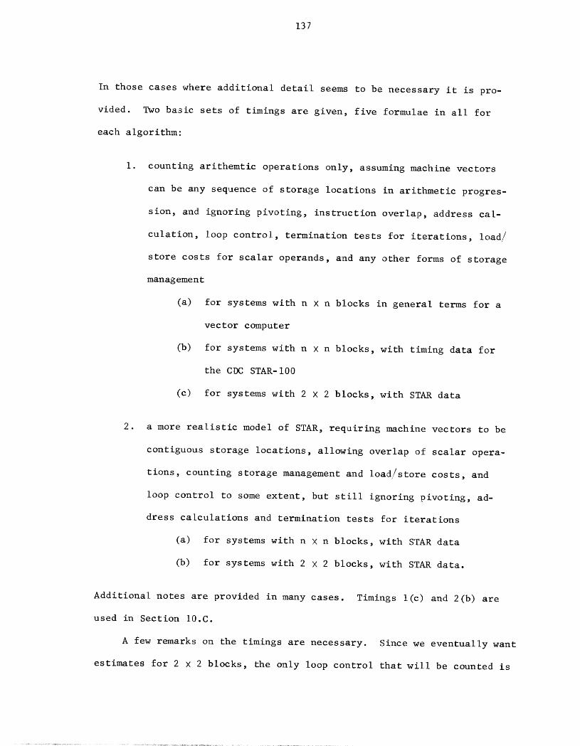
137

In those cases where additional detail seems to be necessary it is pro-

vided. Two basic sets of timings are given, five formulae in all for

each algorithm:

i. counting arithemtic operations only, assuming machine vectors

can be any sequence of storage locations in arithmetic progres-

sion, and ignoring pivoting, instruction overlap, address cal-

culation, loop control, termination tests for iterations, load/

store costs for scalar operands, and any other forms of storage

management

(a) for systems with n × n blocks in general terms for a

vector c_nputer

(b) for systems with n X n blocks, with timing data for

the CDC STAR-100

(c) for systems with 2 X 2 blocks, with STAR data

2. a more realistic model of STAR, requiring machine vectors to be

contiguous storage locations, allowing overlap of scalar opera-

tions, counting storage management and load/store costs, and

loop control to some extent, but still ignoring pivoting, ad-

dress calculations and termination tests for iterations

(a) for systems with n X n blocks, with STAR data

(b) for systems with 2 X 2 blocks, with STAR data.

Additional notes are provided in many cases. Timings l(c) and 2(b) are

used in Section 10.C.

A few remarks on the timings are necessary. Since we eventually want

estimates for 2 × 2 blocks, the only loop control that will be counted is

138

that on the main loops. Operations on n X n matrices or n-vectors are

assumed to be expanded into straightline code.

The address calculations that have been ignored here would be exe-

cuted in scalar mode, and probably can be completely overlapped with

scalar arithmetic operations in the LU factorization. Their effect on

the odd-even methods would be to increase the O(m) terms, m = Flog2N], but

this probably represents only a small relative increase since the O(m)

terms consist of vector startup costs and are already large. While scalar

operations can sometimes destroy the efficiency of a vector code, we be-

lieve that our basic conclusions will not be altered by including address

calculations.

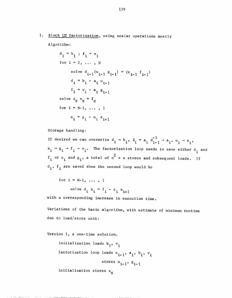
139

I. Block LU factorization, using scalar operations mostly

Algorithm:

dl = bl ; fl = Vl

for i = 2, ... , N

solve di_l(Ui_ I gi_l ) = (ci_ I fi_l )

d i = b i - ai ui_ I

fi = vi - ai gi-i

dN = fsolve xN N

for i = N-I, ... , I

xi gi ui Xi+l

Storage handling :

If desired we can overwrite d i -_ bi, 2. a d-I= -_ a i u -_ ci,l i i-i ' i

xi -_ gi -_ fi -_ vi. The factorization loop needs to save either di and2

f. or u° and gi' a total of n + n stores and subsequent loads. Ifi l

d., f. are saved then the second loop would bel l

for i = N-I, ... , i

solve di x i fi ci Xi.l

with a corresponding increase in execution time.

Variations of the basic algorithm, with estimate of minimum runtime

due to load/store unit:

Version I, a one-time solution.

initialization loads bl, v I

factorization loop loads Ci.l, ai, bi, vi

stores ui_ I, gi-I

initialization stores xN

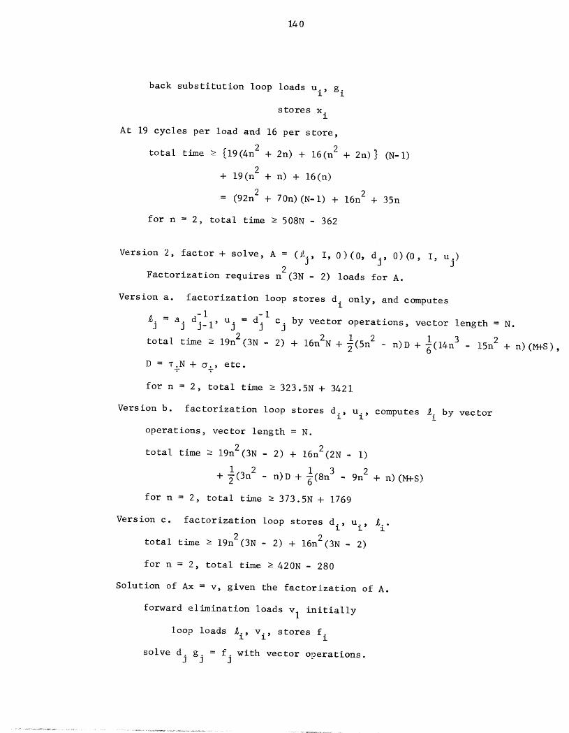
140

back substitution loop loads ui, gi

stores x.l

At 19 cycles per load and 16 per store,

total time _ {19(4n2 + 2n) + 16(n2 + 2n)} (N-l)

2+ 19(n + n) + 16(n)

= (92n2 + 70n)(N-1) + 16n2 + 35n

for n = 2, total time >-508N - 362

Version 2, factor + solve, A = (_j, I, 0)(0, dj, 0)(0, I, uj)2

Factorization requires n (3N- 2) loads for A.

Version a. factorization loop stores d. only, and computesi

-I -i

_j = aj dj_ I, uj = dj c.0 by vector operations, vector length = N.

I i 3total time _ 19n2(3N- 2) + 16n2N + (5n2 - n)D + _(14n - 15n2 + n)(M+S),

D = T.N + _., etc.

for n = 2, total time >-323.5N + 3421

Version b. factorization loop stores di, ui, computes %°Iby vector

operations, vector length = N.

total time >- 19n2(3N - 2) + 16n2(2N - I)

I _ i+ _(3n 2 n)D + _(8n 3 - 9n2 + n)(M+S)

for n = 2, total time _ 373.5N + 1769

Version c. factorization loop stores di, ui, _''l

total time >- 19n2(3N- 2) + 16n2(3N- 2)

for n = 2, total time > 420N - 280

Solution of Ax = v, given the factorization of A.

forward elimination loads vI initially

loop loads _i' vi' stores f.i

solve dj gj fj with vector o_erations.

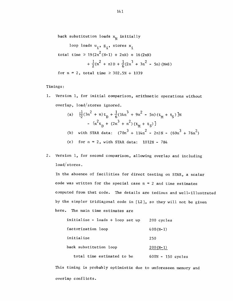
141

back substitution loads xN initially

loop loads ui, gi' stores x.l

total time e 19(2n 2(N-I) + 2nN) + 16(2nN)

1 2 1+ _(n + n)D + v(2n3 + 3n2 - 5n) (M+S)

for n --2, total time ->302.5N + 1039

Timings :

i. Version I, for initial comparison, arithmetic operations without

overlap, load/stores ignored.

(a) [I(3n2 + n)t D + I(14n3 + 9n2 - 5n)(t M + _)}N

- [n2tD + (2n3 + n2)(tM + ts) .}

(b) with STAR data: (70n3 + l14n2 - 2n)N - (60n3 + 76n 2)

(c) for n = 2, with STAR data: 1012N - 784

2. Version I, for second comparison, allowing overlap and including

load/s tores.

In the absence of facilities for direct testing on STAR, a scalar

code was written for the special case n = 2 and time estimates

computed from that code. The details are tedious and well-illustrated

by the simpler tridiagonal code in [L2], so they will not be given

here. The main time estimates are

initialize - loads + loop set up 200 cycles

factorization loop 400(N- I)

initialize 250

back substitution loop 200(N-I)

total time estimated to be 600N - 150 cycles

This timing is probably optimistic due to unforeseen memory and

overlap conflicts.

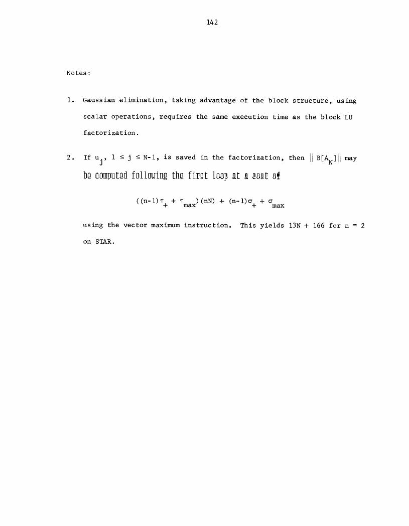
142

Notes :

I. Gaussian elimination, taking advantage of the block structure, using

scalar operations, requires the same execution time as the block LU

factor izat ion.

2. If u., 1 _ j _ N-I, is saved in the factorization, then ]]B[AN]I]..may

3

bna0mDutndf011ooin_thafirst18oDat n as_E 8_

((n-l)_+ + Tmax)(nN) + (n-l)_+ + ¢_max

using the vector maximum instruction. This yields 13N + 166 for n = 2

on STAR.

143

2. Odd-even elimination, using vector operations

We give the algorithm and timing for N = 2m - I, deriving formulae

solely in terms of N and m. Timing for other values of N is approximated

by setting m = rlog2N].

Algorithm: a (I) = a., etc.J J

for i = 1,2,...,m (r = 2i-i) vector

!ensthsfor each j = 1,2,...,N

solve b (i)(_j _(J q0j) - (a (i) (i) (i)• . c. v. ) N, N-rJ J 3 3

take ej = _{j 0, q0j 0 if j < 1 or j > N

b (i+l) b (i) (i) (i). = . - a. - c. N-r3 3 j _j-r j _j+r

v. (i+l) (i) (i) (i)= v. - a. e0. - c. N-rJ 3 j 3-r j _j+r(i+l) _ (i)

a. - -a. _. N-2rJ J j-r(i+l) (i)

cj = -c. N-2rj _j+r

for each j = 1,2,...,N

solve b (m+l) x = v (m+l)3 J 3

Storage handling: temporary vectors are needed for the factorization of

b.(i)j and for _j, _j, q0jcomputed at each stage, and we can overwrite

b (i+l)_, b (i) (i+l) (i)• , a. -* a. , etc.J ] 3 3

Timing :

i. arithmetic only

1(a) [l(5n2 + n)TD + _ (38n3 + 3n2 5n) TM

+ 6(38n3 - 9n2 - 5n) TS]Nm

1+ [I(5n2 + n)o D + _(38n 3 + 3n2 5n)_ M

+ _(38n Z 9n2 5n)_ S) ] m

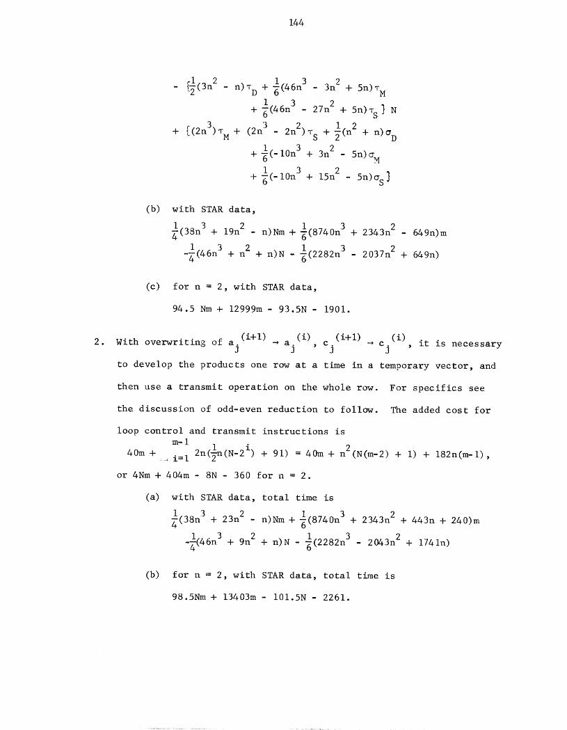
144

- [I(3n2 - n) TD + _(46n 3 3n2 + 5n) TM

I+ _(46n 3 27n 2 + 5n) TS} N

i

+ _(2nB) TM .+ (2n3 - 2n2) TS + _(n2 + n)_ D

1+ _(-10n 3 + 3n2 5n)_M

1_+_(-10n 3 + 15n2 5n)_ S }

(b) with STAR data,

I

I(38n34 + 19n2 " n)Nm + _(8740n 3 + 2343n 2 - 649n)m

i 2 I- (46n3 + n + n)N - _(2282n 3 - 2037n 2 + 649n)

(c) for n = 2, with STAR data,

94.5 Nm + 12999m- 93.5N- 1901.

(i+l) (i) (i+l) (i)2. With overwriting of a. -_a. , c. -_ c. , it is necessary

] ] ] ]

to develop the products one row at a time in a temporary vector, and

then use a transmit operation on the whole row. For specifics see

the discussion of odd-even reduction to follow. The added cost for

loop control and transmit instructions ism-I

I = n240m + ......i=1 2n(_n(N-2 i) + 91) 40m + (N(m-2) + I) + 182n(m-1),

or 4Nm + 404m - 8N - 360 for n = 2.

(a) with STAR data, total time is

1 23n 2 1_(38n 3 + - n)Nm + _(8740n 3 + + 443n + 240)m

2343n 2

-I(46n3- + 9n2 + n)N - --I(2282n3- 2043n 2 + 174 In)u

(b) for n = 2, with STAR data, total time is

98.5Nm + 13403m - 101.5N - 2261.

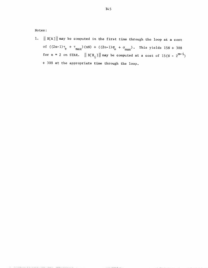
145

Notes :

I. I[B[A]II may be computed in the first time through the loop at a cost

of ((2n-l)_+ + Tmax) (nN) + ((2n-l)_+ + _nax ) . This yields 15N + 308

for n = 2 on STAR. IIB[Hi][l may be computed at a cost of 15(N- 2m-i)

+ 308 at the appropriate time through the loop.

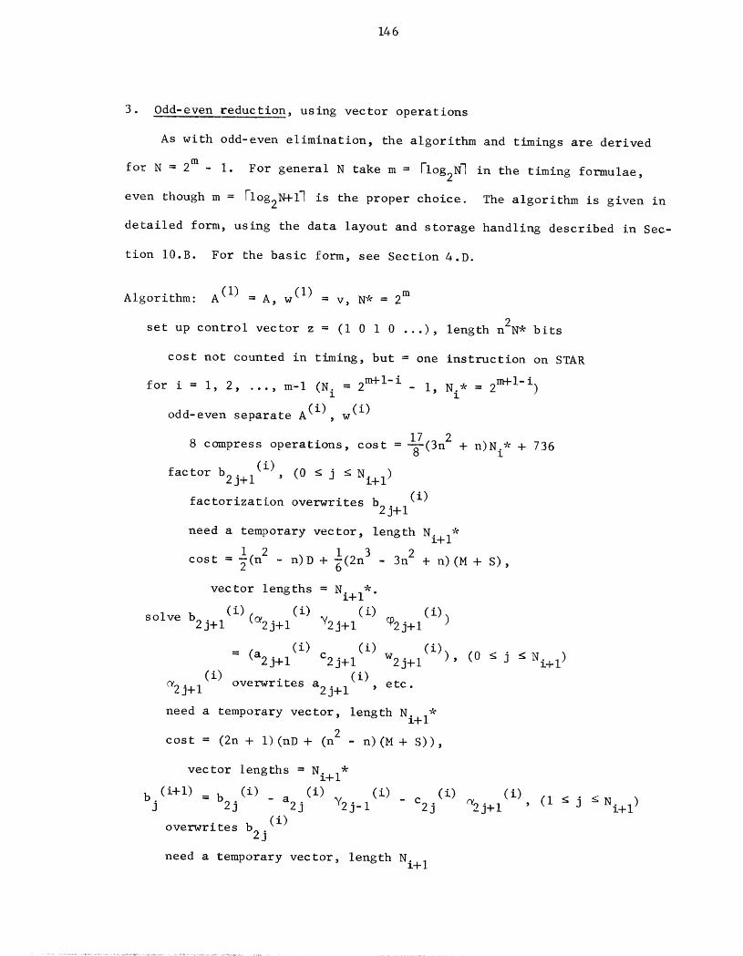
146

3. Odd-even reduction, using vector operations

As with odd-even elimination, the algorithm and timings are derived

for N - 2m - I. For general N take m = rlog2N_ in the timing formulae,

even though m = Flog2N+l] is the proper choice. The algorithm is given in

detailed form, using the data layout and storage handling described in Sec-

tion 10.B. For the basic form, see Section 4.D.

Algorithm: A (I) = A, w (I) = v, N* = 2m

set up control vector z = (i 0 1 0 ...), length n2N * bits

cost not counted in timing, but = one instruction on STAR

for i = I, 2, ..., m-I (Ni = 2m+l-i - I, Ni* = 2m+l-i)

odd-even separate A (i), w(i)

8 compress operations, cost = _(3n 2 + n)N.*l + 736

(i)factor b2j+l , (0 _ j _ Ni+ I)

(i)factorization overwrites b2j+l

need a temporary vector, length Ni+l*

1 2 I

cost = _(n - n) D + _(2n 3 - 3n2 + n)(M + S),

vector lengths - Ni+ 1 .

(i) (i) (i) (i)

solve b2j+l (_2 j+l V2j+I %°2j+l )

(i) (i) (i)

= (a2j+l c2j+l w2j+l ), (0 _ j _ Ni+ I)

(i) (i)

_2j+l overwrites a2j+l , etc.

need a temporary vector, length Ni+l*

cost = (2n + I) (nD + (n2 - n)(M + S)),

vector lengths = Ni+l*

b (i+l) (i) (i) (i) _ c2 (i) (i)j = b2j - a2j V2j-I j _2j+l , (I < j _Ni+ I)

overwrites b2j(i)

need a temporary vector, length Ni+ I

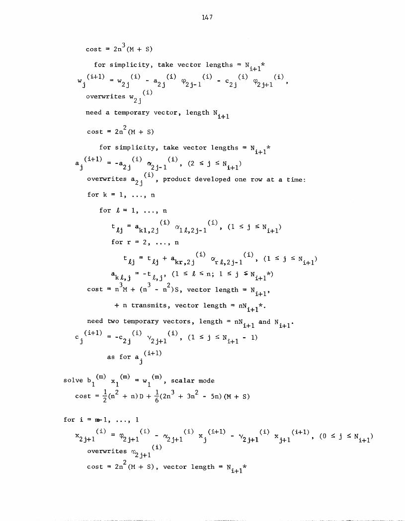
147

cost = 2n3(M + S)

for simplicity, take vector lengths = Ni+l*

(iq-l) (i) (i) (i) (i) (i)w. = w 2 - a2 - c2j j j q°2j- I j q02j+ i '

(i)overwrites w 2 j

need a temporary vector, length Ni+ I

cost = 2n 2(M + S)

for simplicity, take vector lengths = Ni+l*

a. (i+l) (i) (i)3 = -a2j _2j-I , (2 _ j _ Ni+ I)

(i) product developed one row at a time-overwrites a2j ,

for k = i, ..., n

for Z = I, ..., n

(i) _I (i) (I < j < Ni+ I)t%j = akl,2 j _,2j-I '

for r = 2, ..., n

= (i) @ (i)t_j t£j + akr,2 j r_,2j-i , (i < j < Ni+ I)

= -t (I _ _ _n; I _ j ¢ Ni+l *)ak£,j _,j'

3 (n3 2 Ni+lcost = n M + - n )S, vector length = ,

+ n transmits, vector length = nNi+ I .

need two temporary vectors, length = nNi+ I and Ni+ I.

c (i+l) =-c2 (i) (i) - i)J j V2j+ I , (I _ j _ Ni+ I

(i+l)as for a.

J

(m) xl(m) = wl(m) scalar modesolve b I

= I 2 Icost _(n + n)D + _(2n 3 + 3n 2 - 5n)(M + S)

for i = m-l, ..., 1

(i) (i) (i) (i+l) (i) (i+l)

x2j+l = _2j+l - _2j+l x.j - _2j+l Xj+l , (0 _ j < Ni+ I)(i)

overwrites ¢D2j+l

cost = 2n2(M + S), vector length - Ni+l*

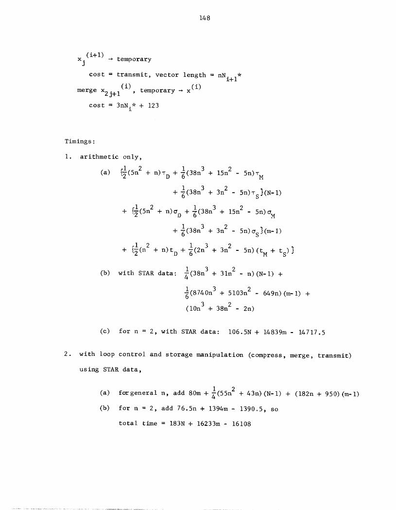
148

(i+1)x. -_ temporaryJ

cost = transmit, vector length = nNi+l*

(i) (i)

merge x2j+l , temporary _ x

cost = 3nNo* + 123i

Timings :

I. arithmetic only,

1

(a) _l(5n2 + n) TD + _(38n 3 + 15n2 - 5n) TM

I

+ _(38n 3 + 3n2 - 5n)Ts }(N-I)

I 2 6(38n3 + 15n2 5n)_M+ [_(5n + n)g D +

1

+ _(38n 3 + 3n2 _ 5n)_s}(m-l)

+ _l(n2 + n) tD + I(2n3 + 3n2 - 5n)(tM + ts) }

i

(b) with STAR data: _(38n 3 + 31n 2 - n)(N-I) +

_i6(8740n3 + 5103n 2 - 649n)(m-l) +

(10n3 + 38n 2 - 2n)

(c) for n = 2, with STAR data: I06.5N + 14839m- 14717.5

2. with loop control and storage manipulation (compress, merge, transmit)

using STAR data,

I

(a) forgeneral n, add 80m + _(55n 2 + 43n) (N-l) + (182n + 950) (m-I)

(b) for n = 2, add 76.5n + 1394m- 1390.5, so

total time = 183N + 16233m- 16108

149

Notes :

i. An estimate for IIB[A]II may be computed in the first time through the

first loop at a cost of ((2n-l)T+ + Tmax)(Nn/2) + ((2n-l)_+ + _max ).

This yields 7.5N + 308 for n = 2 on STAR. The estimate of IIB[A]II is

simply the maximum row sum taken over every other block row. The true

value of II[A]II could be found by computing the remaining rows of B[A],

but this is more expensive and defeats the purpose of odd-even reduction.

150

4. p-fold reduction

m

The algorithm and timings are given for N = p - I, p >-3. For general

m/log 2 - OgpN, take m = FlogpN] - p, m = rlog2N] ; m = rl N+I_ is actually the

proper choice.

m+l-i

Algorithm: (see Section 6.A for details), Ni = p - I.

for i = I, ..., m-I

for each k = I, ..., Ni+ I + I,

LU process on

for each k = I, ..., Ni+ I

UL process on _+I

generate A (i+l) w (i+l)

(m) (m)= wl(m)solve b I Xl

for i = m-l, ..., I

for each k = I, ..., Ni+ 1 + 1

back substitute for Xkp.j , 1 _ j _ p-I

Timing :

1

i. (a) for general n, _(5n2 + n)T D + _(26n 3 + 3n2 - 5n)TM

1 - -

+ _(26n 3 3n2 5n)_ S} (N-p+l)

I+ [5n2 + n)_ D + _(26n 3 + 3n2 5n)_ M

i+ _(26n 3 - 3n2 5n)_s}(m-l) (p-l)

I+ {l(n2 + n) tD + _(2n 3 + 3n2 5n)(tM+t S)}

I

(b) with STAR data, _(26n 3 + - n)(N - p + I)21n 2

+ I(5980n3 + 2769n 2 - 649n) (m-l)(p-l)

+ (10n3 + 38n 2 - 2n)

151

(c) using STAR data, n = 2: 145N + (19206m - 19351)(p-1) + 228

__)- (19351p - 19579)- 145N + 19206m °g2P

2. data manipulation costs are outlined in Section 10.B. We have not

derived the complete timing formulae, as the method is expected to be

too slow.

Notes :

I. In the arithmetic timing, for p e 3, p-fold reduction is always cheaper

than (p+l)-fold reduction for any n. Comparison of 2-fold (odd-even)

and 3-fold reduction yields an N(n) such that if N _ N(n)then odd-even

reduction is faster. Although we have not determined N(n), the block

LU factorization will probably be faster than either _eduction method

for N < N(n). Similar results should hold when overhead costs are

included in the time estimates.

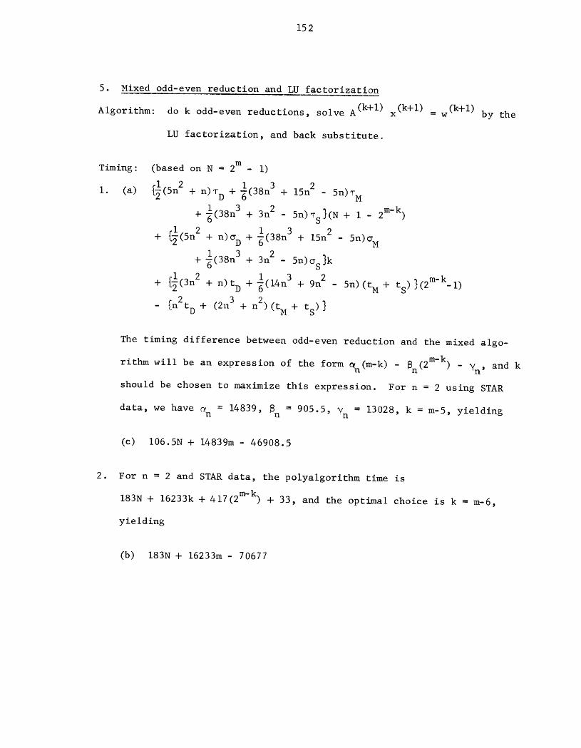
152

5. Mixed odd-even reduction and LU factorization

C ) (k+ i) (k+I)Algorithm- do k odd-even reductions, solve A -k+l- x = w by the

LU factorization, and back substitute.

Timing: (based on N = 2m - I)

i. (a) {I(5n2 + n)T D + I(38n3 + IDn2 - 5n)T M

i+ _(38n 3 + 3n2 5n) Ts}(N + I - 2m-k)

I+ {I(5n2 + n)G D + _(38n 3 + 15n2 5n)G M

I

+ _(38n 3 + 3n2 _ 5n)Gs}k

i+ {i(3n2 + n) tD + _(14n 3 + 9n2 - 5n)(t M + tS) }(2m-k i)

- {n2tD + (2113+ n2)(tM + tS)}

The timing difference between odd-even reduction and the mixed algo-

rithm will be an expression of the form _n(m-k) - _n(2m-k) - _n' and k

should be chosen to maximize this expression. For n = 2 using STAR

data, we have _ = 14839, _ = 905.5, v = 13028, k = m-5, yieldingn n n

(c) I06.5N + 14839m- 46908.5

2. For n = 2 and STAR data, the polyalgorithm time is

183N + 16233k + 417(2 m-k) + 33, and the optimal choice is k = m-6,

yielding

(b) 183N + 16233m - 70677

153

6. Incomplete reduction

[A(k+ (k+l)• (k+l)Algorithm: do k odd-even redmctions, solve D I)] Y = w , and

(I) (1)back substitute to obtain y = y _ x = x.

Timing: (based on N = 2m - I)

I. (a) _I(5n2 . n)TD + I(38n3 + 15n2 - 5n)TM

i

+ _(38n3 + 3n2 - 5n)T S} (N + i- 2re'k)

I+ _i(5n2 + n)_ D + _(38n 3 + 15n2 5n)_ M

I+ _(38n 3 + 3n2 5n)_s}k

1 I - I)+ (n2 + n)T D + _(2n 3 + 3n2 - 5n)(T M + TS) }(2m-k

I 3

+ _l(n2 + n)_ D + _(2n + 3n2 - 5n)(_ M + _S)}

(b) general n, STAR data:

i(38n 3 + 31n 2 - n)N + I(8740n3 + 5103n 2 - 649n)k

- (9n3 + 6n2)(2 m-k - i) + I(460n3 + l191n 2 - 649n)

(c) using STAR data, n = 2: I06.5N + 14839k - 96(2m-k) + 1287

2. (a) general n, STAR data:

I(38n 3 + 86n 2 + 42n)N + I(8740n 3 + 5103n 2 + 443n +5700) k

I

- _(36n 3 + 79n2 + 51n)(2 m'k - I)

I

+ _(460n 3 + l191n 2 - 1651n) + 80(k+l)

(b) n = 2, STAR data:

183N + 16233k- 176.5(2 m-k) + 1113.5

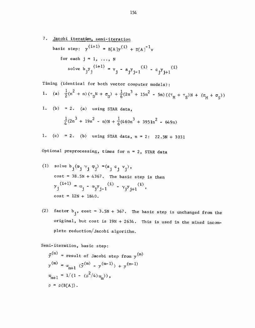
154

7. Jacobi iteration, semi-iteration

basic step: y(i+l) B[A]y(i) + D[A]-I-- V

for each j = I, ..., N

(i+l) _ (i) (i)

solve bjyj -vj - ajyj_ I - cjYj+I

Timing (identical for both vector computer models):

II. (a) _(n 2 + n)(TDN + _D) + 6(2n 3 + 15n2 5n)((T M + _s)N + (_M + _S ))

I. (b) = 2. (a) using STAR data,

l(2n 3 + 19n2 n)N + _(460n 3 + 3951n 2 649n)4

I. (c) = 2. (b) using STAR data, n = 2: 22.5N + 3031

Optional preprocessing, times for n = 2, STAR data

(I) solve bj(_j vj q0j) =(aj cj vj),

cost = 38.5N + 4367. The basic step is then

(i+l) _ (i) (i)

yj -e0j- _jYj-I - VjYj+I '

cost = 12N + 1840.

(2) factor bj, cost = 3.5N + 367. The basic step is unchanged from the

original, but cost is 19N + 2634. This is used in the mixed incom-

plete reduction/Jacobi algorithm.

Semi-iteration, basic step:

_(m) = result of Jacobi step from y(m)

(m-i) (m-I)y(m) = _m+l (9(m) _ Y ) + Y

Wm+ I = i/(I- (p2/4)_n)),

p = p(B[A]).

155

Timing, n = 2, using STAR data: 26.5N + 3408, or 16N + 2217 with the first

preprocessing.

Notes :

I. Varga IV3, p. 139] shows that for Jacobi semi-iteration,

,Ie(i),, < _+_b_(_b_ll--))ii/_" e(0)",

= +- P-----_ 1 ,

(i) (i)e =y - x.

A conservative estimate for the number of iterations needed to obtain

IIe(n) II< 1/Nil e(0) II is n - 21ogN / (-log(_b-l)). It follows that

the execution time for an iterative solution is O(N log N) vs. O(N)

for the better direct methods.

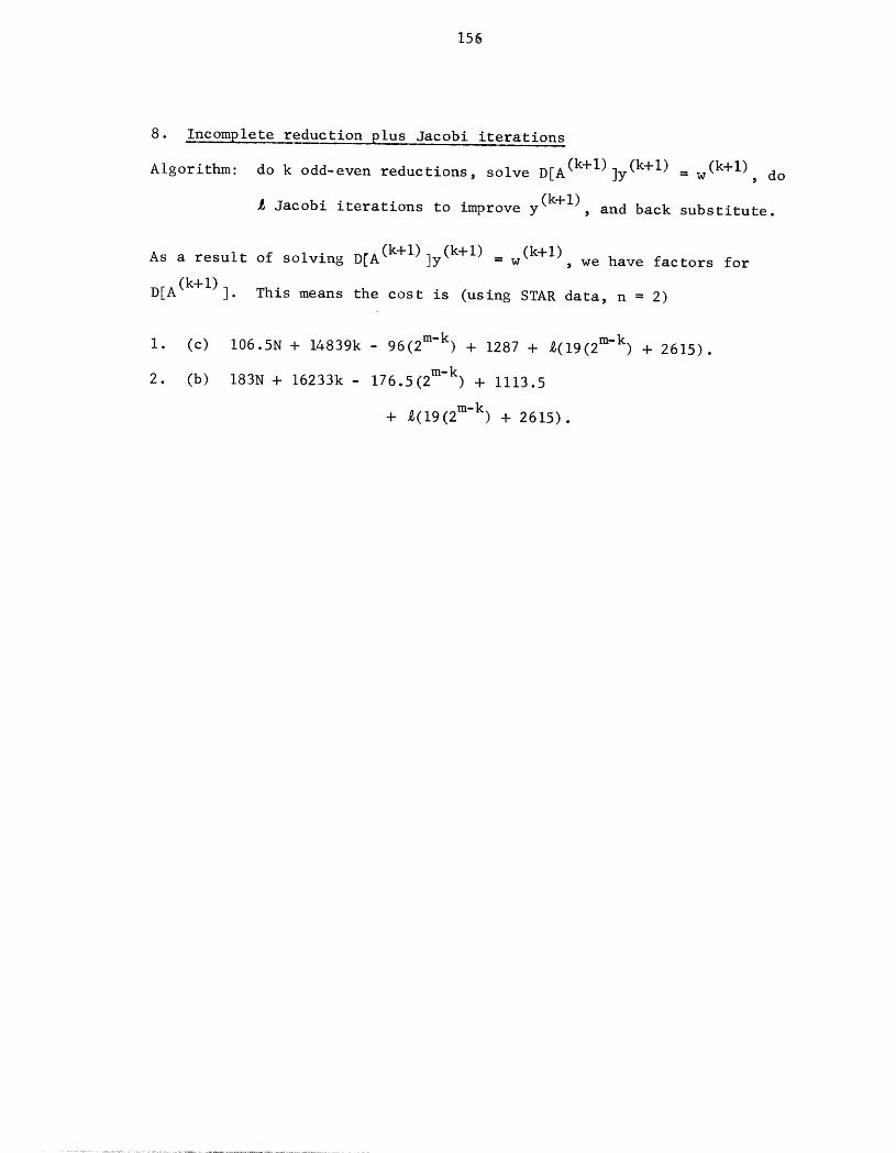
156

8. Incomplete reduction plus Jacobi iterations

(k+l) doAlgorithm: do k odd-even reductions, solve D[A (k+l)]y(k+l) = w ,

(k.l) and back substituteL Jacobi iterations to improve y ,

As a result of solving D[A (k+l) ]y(k+l) w(k+l)= , we have factors for

D[A (k+l) ]. This means the cost is (using STAR data, n = 2)

I. (c) I06.5N + 14839k- 96(2 m-k) + 1287 + %(19(2 m-k) + 2615).

2. (b) 183N + 16233k- 176.5(2 m-k) + 1113.5

+ _(19(2 m-k) + 2615).

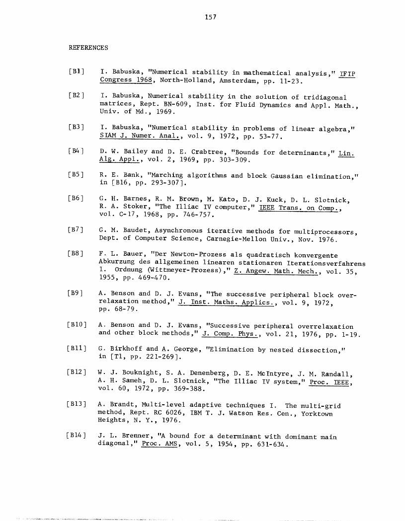
157

REFERENCE S

[BI] I. Babuska, "Numerical stability in mathematical analysis," IFIP

Consress 1968, North-Holland, Amsterdam, pp. 11-23.

[B2] I. Babuska, Numerical stability in the solution of tridiagonal

matrices, Rept. BN-609, Inst. for Fluid Dynamics and Appl. Math.,Univ. of Md., 1969.

[B3] I. Babuska, "Numerical stability in problems of linear algebra,"

SlAM J. Numer. Anal., vol. 9, 1972, pp. 53-77.

[B4] D.W. Bailey and D. E. Crabtree, "Bounds for determinants," Lin.Alg. Appl., vol. 2, 1969, pp. 303-309.

[B5] R.E. Bank, "Marching algorithms and block Gaussian elimination,"

in [BI6, pp. 293-307].

[B6] G.H. Barnes, R. M. Brown, M. Kato, D. J. Kuck, D. L. Slotnick,

R. A. Stoker, "The llliac IV computer," IEEE Trans. on Comp.,vol. C-17, 1968, pp. 746-757.

[B7] G.M. Baudet, Asynchronous iterative methods for multiprocessors,Dept. of Computer Science, Carnegie-Mellon Univ., Nov. 1976.

[B8] F.L. Bauer, "Der Newton-Prozess als quadratisch konvergenteAbkurzung des allgemeinen linearen stationaren Iterationsverfahrens

I. Ordnung (Wittmeyer-Prozess)," Z. Ansew. Math. Mech., vol. 35,1955, pp. 469-470.

[B9] A. Benson and D. J. Evans, "The successive peripheral block over-

relaxation method," J. Inst. Maths. Applics., vol. 9, 1972,pp. 68-79.

[BI0] A. Benson and D. J. Evans, "Successive peripheral overrelaxation

and other block methods," J. Comp. Phys., vol. 21, 1976, pp. 1-19.

[BIll G. Birkhoff and A. George, "Elimination by nested dissection,"

in [TI, pp. 221-269].

[BI2] W. J. Bouknight, S. A. Denenberg, D. E. Mclntyre, J. M, Randall,

A. H. Sameh, D. L. Slotnick, "The llliac IV system," Proc. IEEE,

vol. 60, 1972, pp. 369-388.

[BI3] A. Brandt, Multi-level adaptive techniques I. The multi-gridmethod, Rept. RC 6026, IBM T. J. Watson Res. Cen., Yorktown

Heights, N. Y., 1976.

[BI4] J.L. Brenner, "A bound for a determinant with dominant maindiagonal," Proc. AMS, vol. 5, 1954, pp. 631-634.

158

[BI5] C.G. Broyden, "Some condition number bounds for the Gaussian

elimination process," J. Inst. Maths. Applics., vol. 12, 1973,pp. 273-286.

[BI6] J.R. Bunch and D. J. Rose, eds., Sparse Matrix Computations,Academic Press, N. Y., 1976.

[BI7] B.L. Buzbee, Application of fast Poisson solvers to the numerical

approximation of parabolic problems, Rept. LA-4950-T, Los AlamosSci. Lab., 1972.

[BI8] B.L. Buzbee and A. Carasso, "On the numerical computation of para-

bolic problems for preceding times," Math. Comp., vol. 27, 1973,pp. 237-266.

[BI9] B.L. Buzbee, F. W. Dorr, J. A. George and G. H. Golub, "Thedirect solution of the discrete Poisson equation on irregular

regions," SIAM J. Numer. Anal., vol. 8, 1971, pp. 722-736.

[B20] B.L. Buzbee, G. H. Golub and C. W. Nielson, "On direct methods

for solving Poisson's equations," SlAM J. Numer. Anal., vol. 7,1970, pp. 627-656.

[CI] A. Carasso, "The abstract backward beam equation," SlAM J. Math.Anal., vol. 2, 1971, pp. 193-212.

[C2 ] Control Data Corporation, CDC STAR-100 Instruction execution times,Arden Hills, Minn., Jan. 1976; in conjunction with measurements

made at Lawrence Livermore Laboratory.

[C3] A.K. Cline, personal communication, 1974.

[C4] P. Concus and G. H. Golub, "Use of fast direct methods for the effi-

cient solution of nonseparable elliptic equations," SlAM J. Numer.Anal., vol. I0, 1973, pp. 1103-1120.

[C5] P. Concus, G. H. Golub and D. P. O'Leary, "A generalized conjugate

gradient method for the numerical solution of elliptic partial dif-ferential equations," in [BI6, pp. 309-332].

[C6] S.D. Conte and C. de Boor, Elementary Numerical Analysis, McGraw-Hill, N. Y., 1972.

[C7] M.G. Cox, "Curve fitting with piecewise polynomials," J. Inst.Maths. Applics., vol. 8, 1971, pp. 36-52.

[C8] Cray Research, Inc., "Cray-I Computer," Chippewa Falls, Wis., 1975.

[DI] M.A. Diamond and D. L. V. Ferreira, "On a cyclic reduction method

for the solution of Poisson's equations," SlAM J. Numer. Anal.,vol. 13, 1976, pp. 54-70.

[D2] F.W. Dorr, "The direct solution of the discrete Poisson equation

on a rectangle," SlAM Review, vol. 12, 1970, pp. 248-263.

159

[D3] F.W. Dorr, "An example of ill-conditioning in the numerical solu-

tion of singular perturbation problems," Math. Comp., vol. 25,1971, pp. 271-283.

[El] S.C. Eisenstat, M. H. Schultz and A. H. Sherman, "Applications of

an element model for Gaussian elimination," in [BI6, pp. 85-96].

[E2] D.J. Evans, "A new iterative method for the solution of sparse

systems of linear difference equations," in [R6, pp. 89-100].

[E3] R.K. Even and Y. Wallach, "On the direct solution of Dirichlet's

problem in two dimensions," Computing, vol. 5, 1970, pp. 45-56.

[FI] D.C. Feingold and R. S. Varga, "Block diagonally dominant matricesand generalizations of the Gerschgorin circle theorem," Pacific J.

Math., vol. 12, 1962, pp. 1241-1250.

[F2] D. Fischer, G. Golub, O. Hald, C. Leiva and O. Widlund, "On

Fourier-Toeplitz methods for separable elliptic problems," Math.

Comp., vol. 28, 1974, pp. 349-368.

IF3] G. von Fuchs, J. R. Roy and E. Schrem, "Hypermatrix solution of

large sets of symmetric positive definite linear equations," Comp.Math. in Appl. Mech. and Engng., vol. I, 1972, pp. 197-216.

[GI] J.A. George, "Nested dissection of a regular finite element mesh,"

SIAM J. Numer. Anal., vol. I0, 1973, pp. 345-363.

[HI] L.A. Hageman and R. S. Varga, "Block iterative methods for cyclic-

ally reduced matrix equations," Numer. Math., vol. 6, 1964, pp. 106-119.

[H2] D.E. Heller, "Some aspects of the cyclic reduction algorithm forblock tridiagonal linear systems," SlAM J. Numer. Anal., vol. 13,

1976, pp. 484-496.

[H3] D.E. Heller, A survey of parallel algorithms in numerical linearalgebra, Dept. of Comp. Sci., Carnegie-Mellon Univ., 1976; SlAM

Review, to appear.

[H4] D.E. Heller, D. K. Stevenson and J. F. Traub, "Accelerated itera-tive methods for the solution of tridiagonal systems on parallel

computers," J.ACM, vol. 23, 1976, pp. 636-654.

[H5] R.W. Hockney, "A fast direct solution of Poisson's equation using

Fourier analysis," J.ACM, vol. 12, 1965, pp. 95- 113.

[H6] R.W. Hockney, "The potential calculation and some applications,"

Methods in Computational Physics, vol. 9, 1970, pp. 135-211.

[H7 ] E. Horowitz, "The application of symbolic mathematics to a singularperturbation problem," Proc. ACM Annual Conf., 1972, vol. II,

pp. 816-825.

160

[H8] A.S. Householder, The Theory of Matrices in Numerical Analysis,Blaisdell, N. Y., 1964.

[Jl] T.L. Jordan, A new parallel algorithm for diagonally dominanttridiagonal matrices, Los Alamos Sci. Lab., 1974.

IJ2] M.L. Juncosa and T. W. Mullikin, "On the increase of convergencerates of relaxation procedures for elliptic partial differenceequations," J.ACM, vol. 7, 1960, pp. 29-36.

[KI] W. Kahan, Conserving confluence curbs ill-condition, Dept. of

Comp. Sci., Univ. of Calif., Berkeley, 1972.

"On computing reciprocals of power series,[K2] H.T. Kung, " Numer.

Math., vol. 22, 1974, pp. 341-348.

[K3] H.T. Kung and J. F. Traub, All algebraic functions can be computed

fast, Dept. of Comp. Sci., Carnegie-Mellon Univ., July 1976.

ILl] J.J. Lambiotte, Jr., The solution of linear systems of equations

on a vector computer, Dissertation, Univ. of Virginia, 1975.

[L2] J.J. Lambiotte, Jr. and R. G. Voigt, "The solution of tridiagonal" ACM Trans. Mathlinear systems on the CDC STAR-100 computer,

Software, vol. I, 1975, pp. 308-329.

[MI] N. Madsen and G. Rodrigue, A comparison of direct methods for tri-

diagonal systems on the CDC STAR-100, Lawrence Livermore Lab.:,1975.

[M2] M.A. Malcolm and J. Palmer, "A fast direct method for solving a

" CACM vol 17 1974 pp 14-class of tridiagonal linear systems, __, . , ,17.

• " ACM Trans. Math[M3] W Miller, "Software for roundoff analysis,Software, vol. I, 1975, pp. 108-128.

IN1] A.K. Noor and S. J. Voigt, "Hypermatrix scheme for finite element

" Computers and Structures, volsystems on CDC STAR-100 computer,5, 1975, pp. 287-296.

[01] J.M. Ortega and R. G. Voigt, Solution of partial differentia]:

equations on vector computers, ICASE, Hamton, Va., 1977.

[02] A.M. Ostrowski, "_ber die Determinanten mit _berwiegender Haupt-

diagonale," Comment. Math. Helv., vol. I0, 1937, pp. 69-96.

• "On the stability of Gauss-Jordan[PI] G Peters and J. H. Wilkinson,

elimination with pivoting," CACM, vol. 18, 1975, pp. 20-24.

JR1] J.K. Reid, ed., Larse Sparse Sets of Linear Equations, AcademicPress, London, 1970.

161

JR2 ] J.K. Reid, "On the method of conjugate gradients for the solu-

tion of large sparse systems of linear equations," in [RI,pp. 231-254 ].

[R3] F. Robert, "Blocks-H-matrices et convergence des methods itera-

tives classiques par blocks," Lin. Alg. Appl., vol. 2, 1960,pp. 223-265.

[R4] D.J. Rose and J. R. Bunch, "The role of partitioning in the numer-

ical solution of sparse systems," in JR6, pp. 177-187].

JR5] D.J. Rose and G. F. Whitten, "A recursive analysis of dissection

strategies," in [BI6, pp. 59-83].

[R6] D.J. Rose and R. A. Willoughby, eds., Sparse Matrices and TheirApplications, Plenum Press, N. Y., 1972.

JR7] J.B. Rosser, The direct solution of difference analogs of

Poisson's equation, rep. MRC-TSR-797, Math. Res. Cen., Madison,Wis., 1967.

[SI] J. Schr_der and U. Trottenberg, "Reduktionsverfahren fur Differ-

enzengleichungen bei Randwertaufgaben I," Numer. Math., vol. 22,1973, pp. 37-68.

[Sla] J. SchrSder, U. Trottenberg and H. Reutersberg, "Reduktionsver-

fahren f_r Differenzengleichungen bei Randwertaufgaben II," Numer.Math., vol. 16, 1976, pp. 429-459.

[$2] H.S. Stone, "Parallel tridiagonal equation solvers," ACM Trans.Math. Software, vol. I, 1975, pp. 289-307.

[$3] H.S. Stone, ed., Introduction to Computer Architecture, ScienceResearch Associates, Palo Alto, Calif., 1975.

[$4] G. Strang and G. J. Fix, An Analysis of the Finite Element Method,Prentice-Hail, Englewood Cliffs, N. J., 1973.

[$5] P.N. Swarztrauber, "The direct solution of the discrete Poisson

equation on the surface of a sphere," J. Comp. Phys., vol. 15,1974, pp. 46-54.

[$6] P.N. Swarztrauber, "A direct method for the discrete solution of

separable elliptic equations," SlAM J. Numer. Anal., vol. II,1974, pp. 1136- 1150.

[$7] P.N. Swarztrauber and R. A. Sweet, "The direct solution of the

discrete Poisson equation on a disc," SlAM J. Numer. Anal., vol.I0, 1973, pp. 900-907.

[$8] P. Swarztrauber and R. Sweet, Efficient FORTRAN subprograms for

the solution of elliptic partial differential equations, Rept.

NCAR-TN/IA-109, Nat. Cen. for Atmospheric Res., Boulder, Col.,1975.

162

[$9] R.A. Sweet, "Direct methods for the solution of Poisson's equa-

tion on a staggered grid," J. Comp. Phys., vol. 12, 1973, pp. 422-428.

[Sl0] R.A. Sweet, "A generalized cyclic reduction algorithm," SlAM J.

Numer. Anal., vol. II, 1974, pp. 506-520.

[SIll R.A. Sweet, "A cyclic reduction algorithm for block tridiagonal

systems of arbitrary dimension," contributed paper, Symp. onSparse Matrix Computations, Argonne Nat. Lab., Sept. 1975.

[TI] J.F. Traub, ed., Complexity of Sequential and Parallel NumericalAlgorithms, Academic Press, N. Y., 1973.

IT2] J.F. Traub, "Iterative solution of tridiagonal systems on parallelor vector computers," in [TI, pp. 49-82].

IT3] J.F. Traub, ed., Analytic Computational Complexity, Academic:Press, N. Y., 1976.

IV1] J.M. Varah, "On the solution of block tridiagonal systems arising

from certain finite difference equations," Math. Comp., vol. 26,

1972, pp. 859-868.

IV2 ] J.M. Varah, "A comparison of some numerical methods for two-pointboundary value problems," Math. Comp., vol. 28, 1974, pp. 743-755.

IV3] R.S. Varga, Matrix Iterative Analysis, Prentice-Hall, EnglewoodCliffs, N. J., 1962.

IV4] R.S. Varga, "On recurring theorems on diagonal dominance," Lin.Alg. Appl., vol. 13, 1976, pp. 1-9.

[WI] W.J. Watson, "The TI ASC, a highly modular and flexible super-computer architecture," AFIPS Fall 1972, AFIPS Press, Montvale,

N. J., vol. 41, pt. I, pp. 221-229.

[W2] O.B. Widlund, "On the use of fast methods for separable finitedifference equations for the solution of general elliptic problems,"

in JR6, pp. 121-131].

[W3] J.H. Wilkinson, "Error analysis of direct methods of matrix inver-sion," J.ACM, vol. 8, 1961, pp. 281-330.

[W4] W.A. Wulf and C. G. Bell, "C.mmp, a multi-mini-processor," AFIPSFall 1972, AFIPS Press, Montvale, N. J., vol. 41, pt. 2, pp. 765-777.

[yl] D.Y.Y. Yun, "Hensel meets Newton - algebraic constructions in an

analytic setting," in IT3, pp. 205-215].