Direct and Indirect use of Fossil Fuels in Farming: Cost of … 1. Introduction This paper focusses on the interaction between fossil fuels and farming in India, to capture total intensity

1

Direct and Indirect use of Fossil Fuels in Farming: Cost of

Fuel-price Rise for Indian Agriculture

Mukesh Anand

Working Paper No. 2014-132

February 2014

National Institute of Public Finance and Policy

New Delhi

http://www.nipfp.org.in

2

Direct and Indirect Use of Fossil

Fuels in Farming: Cost of Fuel-

price Rise for Indian Agriculture

Mukesh Anand

Abstract

A hornet’s nest could be an apt simile for fossil fuel prices in India. Over years

a policy maze has evolved around it, with sharply diverging influence on

disparate constituencies.1 We estimate the increase in total cost of farming as a

multiple of direct input costs of fossil fuels in farming. Over the period

between 1990-1 and 2010-1, direct use of fossil fuels on farms has risen and

there is also increasing indirect use of fossil fuels for non-energy purposes.

Consequently, for Indian agriculture both energy intensity and fossil fuel

intensity are rising. But, these are declining for the aggregate Indian economy.

Thus, revision of fossil fuel prices has acquired greater significance for Indian

agriculture than for the remainder of the economy. We validate these findings

by utilising an input-output table for the Indian economy to assess the impact

of fossil fuel price increase. We assess that fossil fuels sector has strong

forward linkages and increase in its price has a steep inflationary impact.

Using a three-sector I-O model for Indian economy, we estimate that a 10 per

cent increase in fossil fuel price could cause, mutatis mutandis, the wholesale

price index (WPI) to rise about 4.3 percentage points with 0.7 percentage

points being contributed by the farm sector alone.

Keywords: Agriculture, Fossil-fuel intensity, Inflation, Input-Output analysis

JEL Classification: C67, E31, Q12, Q43

Assistant Professor, National Institute of Public Finance and Policy (NIPFP), New Delhi,

India; [email protected]; The idea contained in this paper was presented at two

conferences, on (a) Fossil Fuels in Agriculture: Impact on India’s Farmers, at India

International Centre Annexe on March 26, 2013 organised by Bharat Krishak Samaj, and, (b)

Hydrocarbons: India’s Regulatory Dilemma: Too Much or Too Little?, 12th

Petro India 2013

at India International Centre, Multipurpose Hall on December 11, 2013 organised by India

Energy Forum. I thank Indira Rajaraman (member, Thirteenth Finance Commission) and

Rathin Roy (Director, NIPFP) for their suggestions on a draft version. 1 Formed along differing dimensions these constituencies may or may not overlap, like

agriculture, industry or services, upstream or downstream companies, public or private sector,

households or commercial consumers etc.

mailto:[email protected]

3

1. Introduction

This paper focusses on the interaction between fossil fuels and farming in

India, to capture total intensity of fossils in farming and offer some evidence

on inflationary impact of fossil fuel price increase in India.

Revision of fossil fuel2 prices in India continues to be a political hot potato.

This paper is motivated by the often repeated conjecture that, the increase in

prices of fossil fuels could have a significantly large indirect or later-round

impact than direct or first-round impact, on prices in general and food prices

in particular.3

A recent report on pricing diesel (Anand, 2012)4 in India, among other things

discussed very briefly the input cost of diesel / petroleum products. However,

it made only a passing reference to Indian agriculture with a couple of crop-

specific examples. Anand (op. cit.) concerned itself with direct use5 of only

diesel in farming,6 but indirect use of fossil-fuels for farming appears to be

significant.7

2 While fossil is a generic term signifying remains, the term fossil-fuels is often used to denote

products and by-products derived from coal, lignite, crude petroleum, and natural gas.

However, the term fuel is pertinent only when used for deriving energy from their combustion. 3 As per a newspaper report in August 2012, the then governor of Reserve Bank of India

(RBI) D. Subbarao conjectured, that elimination of fuel subsidy could cause a 2.6 per cent

spike in inflation (http://articles.economictimes.indiatimes.com/2012-08-

07/news/33083665_1_food-inflation-fuel-subsidy-governor-d-subbarao). RBI (2011, pp 641)

reports that,

“Empirical estimates show that every 10 per cent increase in global crude

prices, if fully passed-through to domestic prices, could have a direct

impact of 1 percentage point increase in overall WPI inflation and the total

impact could be about 2 percentage points over time as input cost increases

translate to higher output prices across sectors”. 4 Titled Diesel Pricing in India: Entangled in a Policy Maze, this report may be downloaded

from http://www.nipfp.org.in/newweb/sites/default/files/Diesel%20Price%20Reform.pdf;

Working Paper version at

http://www.nipfp.org.in/newweb/sites/default/files/WP_2012_108.pdf 5 Direct use (of fossil fuels) essentially concerns direct purchase of diesel by farmers.

6 See in particular, section 7.5 in Anand (2012).

7 The distinction between fuel and non-fuel (respectively, energy and non-energy) use of

fossils, while important, is not a core concern. Table 51, GoI (2012), pp 48, lists the major

end-uses of petroleum products. The ones relevant for farming and agriculture are (a) Naphtha

/ NGL (natural gas liquid): Feedstock / fuel for fertiliser units, feedstock for petrochemical

sector, and fuel for power plants; (b) HSD (high speed diesel): Fuel for transport sector

(railways / road), agriculture (tractor, pump sets, threshers, etc.), and captive power

generation; (c) LDO (light diesel oil): Fuel for agricultural pump sets, small industrial units,

start-up fuel for power generation; (d) FO / LSHS (fuel oil / low sulphur heavy stock):

Secondary fuel for thermal power plants, fuel / feedstock for fertilizer plants, industrial units.

http://www.nipfp.org.in/newweb/sites/default/files/Diesel%20Price%20Reform.pdf



4

Two important indirect linkages of fossil-fuels and farming are through use of

(a) fertilisers and (b) power or electricity. Natural gas (NG) and naphtha, apart

from furnace oil and other heavy distillates, are commonly used as feedstock

(raw material) in production of fertilisers.8 Coal, diesel, and liquefied NG

(LNG) are used as fuel for electricity (thermal-power) generation for supply to

(a) consumers including farmers, to power their irrigation pump-sets and other

farm-equipment and (b) industry, as input to produce those pump-sets, farm-

equipment, fertilisers, pesticides, and other inputs or raw-materials used on

farms.

In the next section, we briefly recapitulate fossil fuel use at the aggregate

economy level highlighting the proportion of final consumption in agriculture

sector.9 In section 3 we explore some rudimentary evidence on the (direct)

input cost of fossil fuels (essentially diesel) in farming. The available evidence

with some supporting assumptions are then used in section 4 to estimate the

direct impact of an increase in diesel prices on farming operations for differing

crops. The use of fossil-fuels as raw material for manufacture of fertilisers,

almost exclusively used on farms, is discussed in section 5. Use of fossils to

derive thermal energy that is consumed on farms, while energising irrigation

pump-sets and certain farm equipment, is estimated in section 6.10

The

disparate components from sections 3 to 6 are pieced together in section 7.

Next, the deep linkages between fossil fuels and farming are explored using an

alternative approach that employs an input-output (I-O)11

table for the Indian

economy. This is conducted at two levels.12

First, in section 8, a 130-sector

In the approach adopted in this paper direct use constitutes of b and c, while a and d constitute

indirect use. 8 This constitutes one of the non-energy or non-fuel uses of fossils. The euphemistically called

fossil-fuels may be put to non-energy (non-fuel) uses in several other processes. For example,

coal is used as feedstock in making steel as well as in some other industries. 9 There is almost total overlap between final consumption of fossil fuel in agriculture and

direct use of diesel on farms. 10

However, note that thermal power to energise the production processes in industries for

manufacture of fertilisers, pesticides, farm equipment or other such inputs used on farms, is

not estimated here. Although important, the complexity rises sharply with every level of detail

or, as one we go further back in value chain. In any case, this can only add to the total

intensity (of fossil fuels in agriculture) that we seek to estimate. 11

I-O tables for the Indian economy are prepared by the National Accounts Division (NAD)

of the Central Statistics Office (CSO) of the Ministry of Statistics and Programme

Implementation (MoSPI) of the Government of India (GoI). Starting with the publication of

the first I-O tables for 1968-9, the NAD has published a detailed I-O table almost every five

years. The latest in the series pertains to 2007-8 and was published in October, 2012. Until

1998-9 the detailed tables were constructed for 115 sectors classification, but the level of

detail was raised to 130 sectors in 2003-4. 12

It may be a useful exercise to decipher use of fossil fuels through input of power

(electricity) on farms to run farming equipment, or when used in industrial-production of

5

I-O table for Indian economy is aggregated into three sectors representing (i)

farming, (ii) fossil fuels, and (iii) rest of the economy. And second, in section

9, the farming sector is again disaggregated into 15 sectors to decipher the

varying impact of fossil fuel price change on differing crops. Finally, section

10 summarises the paper.

2. Aggregate energy consumption in India and direct use

(final consumption) of fossil-fuels (diesel) on Farms

Energy intensity, estimated as available commercial energy in kilogram of oil

equivalent (kgoe) per thousand Indian rupees (INR) of gross domestic product

(GDP),13

increased from 12.3 in 1980-1 to 14.9 in 1991-2. But since then, has

secularly declined to reach 10.9 in 2009-10.14

Such a situation may transpire

from a combination of the following, (a) the use of fossil fuels may be

displacing use of non-fossil fuels (like firewood, dung-cake), (b) heat energy

from burning of fossil-fuels may be easier to harness and redirect, and (c)

technological developments may raise the efficacy of energy derived from

fossil-fuels.

Data collated from the international energy agency (IEA) on energy balance

corroborates that energy intensity of GDP has declined to almost half its level

in 1990-1 (Column 4, Table 1). Estimates on total primary energy supply

(Column 2, Table 1) also depict a declining trend at the aggregate level. But

the proportion of fossil fuels in total primary energy supply has risen from

close to 50 per cent to above 75 per cent (cf. columns 2 and 3). In 1990-1,

energy intensity of agricultural GDP (cf. columns 4 & 5, Table 1) was only 7

per cent of that for the economy as a whole. But, in 2011-2, this ratio had risen

to 28 per cent and in absolute terms energy intensity of agricultural GDP is

those equipment as well as farm inputs like fertilisers, pesticides. However, this is not

attempted here as unlike in case of fertilisers that are almost exclusively used on farms, power

is an input into a much wider range of economic activities. 13

GDP at constant 2004-5 prices from http://mospi.nic.in/Mospi_New/upload/NAS13.htm. 14

As per GoI (2013, pp 42), energy intensity measured as amount of energy for generating

one unit of GDP (at 1999-2000 prices) increased from 0.128 KWh in 1970-1 to 0.165 KWh in

1985-6. This came down to 0.148 KWh (at 2004-5 prices) in 2011-2. It may however be noted

that because of differing base years for reporting GDP, energy intensity figures for 2011-2 are

not strictly comparable over the entire period as presented in GoI (2013). In another context,

energy intensity of GDP is also expressed as available commercial energy per unit of real

GDP (see, CMIE (2013), TERI (2012)). This is estimated using data on available commercial

energy in million tonnes of oil equivalent (MTOE) and GDP at factor cost at 2004-5 prices in

crore INR. Analogous interpretation is adopted while referring to diesel or petroleum-products

intensities of GDP.

http://mospi.nic.in/Mospi_New/upload/NAS13.htm

6

almost double its value in 1990-1. In India thus, energy intensity for aggregate

GDP is declining but energy intensity of agricultural GDP is rising.

Table 1: Energy Consumption and GDP in India

Year

Primary Energy

Supply in kgoOE per

1000 INR of GDP

Final Consumption of

Energy in kgoOE per 1000

INR of GDP of

GDP at

Constant 2004-

5 Prices at

Factor Cost

(crore INR)

Share of

Agriculture

in GDP at

2004-5 Prices,

(%) Total Fossil Fuels Economy Agriculture

(1) (2) (3) (4) (5) (6) (7)

1990-1 23.50 13.01 18.67 1.40 1347889 29.5

1998-9 20.22 12.81 14.49 2.37 2087828 24.4

2001-2 18.79 12.21 12.85 2.01 2472052 22.4

2007-8 15.52 10.75 10.29 2.40 3896636 16.8

2010-1 14.66 10.62 9.61 2.65 4937006 14.5

2011-2 14.29 10.33 9.39 2.64 5243582 14.1

Source: GDP data from http://mospi.nic.in/Mospi_New/upload/NAS13.htm;

Energy balance data from International Energy Agency

http://www.iea.org/statistics/statisticssearch/report/?country=INDIA&product=balan

ces&year=1990


ces&year=1998


ces&year=2001


ces&year=2007


ces&year=2011

Notes: kgoOE denotes kilogram of oil equivalent; INR denotes Indian rupee; One crore

equals 10 million or 100 lakhs. Column 5 does not include the non-energy use of

fossil fuels, say as feedstock for production of fertilisers, and energy utilised in

production of fertiliser, pesticides, farm equipment, and other farm inputs that are

likely accounted for under industry.

Data collated from alternative sources and presented in table 2 confirm the

above observation. Row 5, table 2 shows that GDP growth (6.72) is relatively

steeper than growth in consumption of fossil fuels, either as a group (5.12) or

individually. 15

Therefore, energy efficiency at the macro-aggregate level and

fossil-fuel intensity of GDP has improved.16

A sharply divergent assessment however, may be concluded if one were to

consider a relatively longer period starting from 1974-5.17

Between 1974-5

15

The decline in fossil fuel intensity is corroborated, but there are differences with respect to

the magnitudes. For example, the 1990-1 estimate for fossil fuels is 16.09 kgoOE per 1000

INR of GDP (against 13.01 as per IEA) and 13.25 for 2007-8 (against 10.75 as per IEA). 16

However, decline in energy-intensity or enhancement of thermal efficiency at the aggregate

level should not be an excuse for complacency in efforts to reduce fossil fuel consumption. 17

There is no ostensible reason for the choice of these initial years, except the ease of

availability of data in the case of former, and in the latter to allow a comparison with publicly


http://www.iea.org/statistics/statisticssearch/report/?country=INDIA&product=balances&year=1990


7

and 2010-1, real GDP (at constant 2004-5 prices) has grown at 5.71 per cent

per annum (Row 3, Column 8, Table 2). Over that period, fossil fuel

consumption consisting of coal, lignite, petroleum products and natural gas

grew at 5.78 per cent per annum (Row 3, Column 6, Table 2). It thus appears

that fossil fuel intensity of GDP may have risen or remained unchanged

between 1974-5 and the present.18

Table 2: Trend growth rates, in consumption of fuels and of GDP,

1970-1 to latest available Period Coal

Offtake

Lignite

Despatch

Petroleum

Products

Natural

Gas

Total

Fossil

Fuel

Diesel GDP at

constant

2004-5

prices

(1) (2) (3) (4) (5) (6) (7) (8)

1970-1 to Latest 5.50 7.44 5.47 11.86 5.75 - 5.52

1974-5 to Latest 5.50 7.68 5.51 11.32 5.78 6.19 5.78

1974-5 to 2010-1 5.50 7.57 5.63 11.56 5.78 6.25 5.71

1990-1 to Latest 5.00 4.49 5.02 5.93 5.12 4.64 6.80

1990-1 to 2010-1 5.00 4.41 5.26 5.96 5.12 4.38 6.72

Source: CMIE, MoSPI, MoPNG

Notes: One million tonne of coal equals 0.67 mtoe. One million tonne of lignite equals 0.33

mtoe. 1 billion cubic metres of natural gas equals 0.9 mtoe. One million tonne of all

refined petroleum products equals one mtoe. Data on ‘latest’ year pertains to (a)

2010-1 for coal and total fossil fuels; (b) 2011-2 for lignite, natural gas, and GDP; (c)

2012-3 for petroleum products, diesel, and GDP.

Further, while relative intensity of lignite and natural gas with respect to GDP

had risen, it declined on account of coal and petroleum products. However,

within the class of petroleum products diesel consumption grew at 6.25 per

cent per annum (Row 3, Column 7, Table 2). Consequently, diesel-intensity of

GDP appears to have risen significantly.19

This has found resonance elsewhere

available IEA data (as in table 1). Fortuitously, though 1990-1 and 1991-2 are often

considered as watershed years in Indian economic policy orientation. 18

This is not surprising, but often causes sharp differences in perception when assessing

policy outcome, especially in developing economies with evolving institutions. Over

relatively longer intervals, abrupt changes arise merely from differences in understanding,

definition or scope of variables. Often these changes are not systematically documented or

adequately evaluated. It thus appears that, the choice of terminal years, in turn determining the

length of the period, considered for analysis makes a significant difference to the conclusion

on direction of estimated trend on energy intensity. However, we believe that to adopt

appropriate policy response, it may be justifiable to accord higher significance to signals that

derive from relatively recent changes. 19

Consumption of middle-distillates and all petroleum products grew respectively at 5.21 and

5.58 per cent per annum over 1974-5 and 2011-2.

8

expressing concern over dieselisation (http://www.cseindia.org/dte-

supplement/air20040331/dieselised.htm).20

The introductory section noted that direct use of fossils on farms pertains to

use of diesel to run agricultural machinery (including tractors, harvesters,

combines etc.), water pumps, and generators. Table 3 presents the share of

diesel consumption (columns 3 to 7), juxtaposed to the changing structure of

GDP (columns 8 to 12).

Table 3:Sector-Wise Share of Total Diesel Consumed and GDP (per cent)

Sector Mode

Diesel Consumed GDP

1998

-9

2000

-1

2008

-9

2010

-1

2011

-2

1998-9 2000-1 2008-9

2010-

11 2011-2

(1) (2) (3) (4) (5) (6) (7) (8) (9) (10) (11) (12)

Transportation

Railways 3.8 3.8 4.2 4.0 1.0 1.0 1.0 1.0 1.0

Water 0.6 0.7 1.4 0.9

4.9 5.0 5.6 5.4 5.6 Aviation 0.1 0.1 Negligible

Road 53.0 53.9 59.6 60.4

Industry 10.4 9.9 8.3 8.2 15.4

(9.5)

15.5

(9.5)

15.8

(10.6)

16.2

(11.3)

15.7

(10.9)

Power Generation 6.9 6.8 8.4 8.2 2.3 2.2 2.0 1.9 1.9

Agriculture 19.2 19.8 11.9 12.2 24.4

(20.7)

22.3

(18.7)

15.8

(13.4)

14.5

(12.3)

14.1

(12.0)

Miscellaneous 6.1 6.7 4.3 3.8

Source: GDP by Economic Activity at Constant 2004-5 prices accessed at

http://mospi.nic.in/Mospi_New/upload/NAS_2012_25july12/statements(pdf)/S11.1

.pdf on September 20, 2012. Diesel consumption from

http://petroleum.nic.in/pngstat.pdf, GoI, 2012b.


http://economicoutlook.cmie.com/kommon/bin/sr.php?kall=wshreport&&repcode=

016017015010010010000000000000000000000000000&repnum=12932&prs=000

-999-999-00012930

Notes: GDP data in transportation services is available for ‘railways’ and ‘other transport

services’ the latter includes air and water transport; Share of Industry in GDP

pertains to ‘manufacturing’ (registered (shown in parenthesis) plus unregistered);

Share of Power in GDP relates to ‘electricity, gas and water supply’; Share of

agriculture in GDP includes ‘agriculture (shown in parenthesis), forestry and

fishing’.

20

There is rising rhetoric against risks from single-fuel predominance due to policy induced

technological choices or from dithering energy-price reforms. The number of units of

petroleum products to satisfy a unit increase in average final demand for all sectors, increased

by almost one-third, from 2.991 to 4.0461, between 1983-4 and 2003-4. Anand (op. cit, pp.

37) discussed the strong and intensifying forward linkage of petroleum products / diesel with

rest of the economy, endorsing the steep increase in weight on diesel in the wholesale price

index (WPI). The weight on diesel changed from 2.02034 in 1993-4 series to 4.67020 in 2004-

5 series. The weight on fuels as a group changed from 8.74254 to 11.45858. The weight on

power declined from 5.48369 to 3.45163 (see also table 12 in section 7).

http://petroleum.nic.in/pngstat.pdf


9

Between 1998-9 and 2010-1, the proportion of diesel consumed had risen

significantly in transportation, along with an equi-proportionate rise in its

contribution to GDP. In industry the proportion of diesel consumed has

declined but contribution to GDP has somewhat risen. In case of power the

proportion of diesel consumed has risen but contribution to GDP has

somewhat declined. But, in agriculture the proportion of diesel consumed has

declined and so has the contribution to GDP.

A sharper focus on only recent data indicates a reversal of above trends.

Between 2008-9 and 2010-1, agriculture is the only sector to portray a rise in

share of diesel consumed (from 11.9 to 12.2 per cent) and also a perceptible

decline in share of GDP (from 15.8 to 14.5 per cent). It appears that diesel-

intensity of GDP contributed by different sectors, may have grown differently.

Table 4 presents the relative diesel intensity, and it is observed that, between

1998-9 and 2000-1, relative diesel intensity of GDP increased for both power

and agriculture, but declined for industry and remained almost unchanged for

transportation sectors. In more recent years again, since 2008-9, while relative

diesel intensity of GDP has risen for all sectors, it has grown fastest for

agriculture sector GDP.

Table 4: Relative Diesel Intensity of Sectoral GDP

Year Transportation Industry Power Agriculture

1998-9 9.75 0.68 3.00 0.79

2000-1 9.75 0.64 3.09 0.89

2008-9 10.00 0.65 4.15 0.75

2010-1 10.20 0.65 4.32 0.84

Change During Period (per cent)

1998-9 to 2000-1 0.04 -5.42 3.03 12.84

2000-1 to 2008-9 2.56 1.07 34.26 -15.17

2008-9 to 2010-1 2.03 0.40 3.99 11.71

Source: Author’s own computation

Notes: Industry includes registered and unregistered manufacturing; Agriculture

includes forestry and fishing. Relative intensity is calculated using shares

instead of actual quantity / value and expressed as a ratio of the share of

diesel consumed in the sector to share of GDP contributed by the sector.

Acceleration in relative diesel-intensity of agriculture in comparison to non-

agriculture (including transportation), in part, is indicative of continual

mechanisation of farm labour. But more importantly, it perhaps signals

widespread disappointment with the power sector to satisfactorily address the

rising energy-demand from this sector.21

One may surmise that, in recent

years Indian agriculture is experiencing faster dieselisation than rest of the

21

This issue is revisited in section 6.

10

economy.22

Note the congruence with observations on agricultural sector from

table 1. Further, if correctives are not introduced earnestly, fossil-fuelisation

of Indian agriculture may rise alarmingly.

3. Cost of Agricultural Production

Over the last few years, food price inflation in India has continued to remain at

an elevated level (RBI, 2014). The dominant reason accorded to this persistent

increase in prices, especially of fruits and vegetables, is a demand pull factor

due to growth in incomes (Bandara, 2013). Further, income increase has also

raised the demand for finer cereals and protein-rich food (Ganguly and Gulati,

2013; RBI, 2011a; RBI 2011b). There could hardly be a case to dispute these

arguments.23

On supply side, the minimum support price (MSP) policy periodically

ratchets-up prices garnered by farmers / producers. However, the MSP policy

is necessarily geared to account for input costs incurred by farmers. In that

sense it could be a conduit for cost-push inflation. But, retail prices of several

farm inputs including power, fertilisers, and diesel are also administered (fixed

or influenced) by government policy. In the event of an increase in

international price of crude petroleum or other fossil fuels, the government is

faced with a choice to either allow their passage onto domestic retail prices or

continue to subsidise farm inputs, while compensating the (input) producers of

power, fertilisers, and diesel.

Several government of India (GoI) committees (GoI (2006, Rangarajan), GoI

(2010, Parikh), GoI (2013, Parikh)) constituted over years, have concluded

that in the long run it is desirable to decontrol fossil fuel prices.24

These

committee reports however, have neither indicated the timing for decontrol

nor spelt out the pre-conditions that warrant it. On the contrary, they cemented

the belief that the time (for decontrol) may not be ripe as yet.25

It is believed

22

However, this observation needs to be tempered considering the possibility of abrupt

changes in categorisation of data. The most recent example is the sweeping categorisation of

more than 85 per cent consumption of HSD under Miscellaneous Services for the year 2011-2

(see pg. 73, http://petroleum.nic.in/pngstat.pdf, January 2013). 23

Both, finer cereals and protein-rich food are normal goods at extant average income and

consumption level. 24

This author however opines that full ‘decontrol’ is a myth when the tax component in the

price is significant and in the case of some fossil fuels constitutes close to half of the prevalent

price. 25

This is also reflected in the hesitation of the empowered committee of state finance

secretaries to include all fossil fuels under the ambit of the proposed GST.


11

that while decontrol would lead to immediate increase in prices of essential

items (and hence general inflation), it may have a salubrious influence on long

term growth prospects and price stabilisation (RBI, Bhanumurthy et al (2012),

Bhattacharya and Batra (2009), Bhattacharya and Bhattacharya (2001).

Political constituency for decontrol is however weak, perhaps due to

inadequate mapping of (and therefore estimates for) economy-wide impact of

fossil fuel price revision. In particular, there is paucity of studies in the Indian

context, relating to impact of fossil fuel prices on agriculture. However,

reports of Commission for Agricultural Costs and Prices (CACP) collate costs

of production of several commodities. And, appendix II of GoI (2000)

describes the approaches adopted for estimating various costs under a

comprehensive scheme for studying the cost of cultivation of principal crops.

In one approach, cost data categorised into operational and fixed costs (per

hectare) is collated for specific crops. The operational cost is grouped into

labour (human, animal and machine), material (seeds, fertiliser, manure,

insecticides), and service (irrigation, interest) categories. But, a quick scan

reveals that expenditure incurred on direct purchase of fuels or on purchase of

power, is not shown separately.26

Apparently, operational cost of machine

labour includes costs incurred on fuel and lubricants for mechanised

agricultural implements and equipment including water-pumps. Although

entailing further assumptions, this structure appears convenient for our

purpose to estimate input cost of diesel for differing crops over years.

Cost incurred on purchase of fertilisers and insecticides are also presented, but

again these are retailed to farmers at subsidised rates. Consequently, the

transmission of fossil fuel price revision may not be reflected in farming costs.

The paper attempts to address this gap. It deciphers the direct (as diesel) and

indirect (as in production of fertilisers and power) use of fossil fuels on farms

and then focuses on the likely impact of change in fossil fuel prices on costs of

agricultural production.

26

There is an element of irrigation charges that essentially relates to payment to the irrigation

department for consumption of water on farms.

12

4. Operational cost of machine labour and cost of diesel in

total cost of production

Fortuitously, a one-off table (partly reproduced here as table 5), gives a rough

estimate of diesel cost as a proportion of operational cost of machine labour.27

One observes that diesel cost per hectare varies significantly among crops and

across provinces. This variation is on account of differences in (a) technology,

including adoption of high-yielding variety (HYV) of seeds, degree of

mechanisation, (b) extent of irrigation, (c) accessibility to alternative sources

of energy (mainly electric power), and even (d) price of diesel, that varies

significantly across provinces (mainly due to differences in provincial taxes on

diesel).28

On an average, however for the crops and provinces shown in table

5, diesel accounted for about 62 per cent of operational cost of machine

labour.

Table 5: Diesel Cost in Operational Cost of Machine Labour, INR per

Hectare, 1998-9

Crop Province Diesel

Cost

Op. Cost of

Mach. Lab.

col. 3 / col. 4

(per cent)

1 2 3 4 5

Wheat

Haryana 1044.8 1958.41 53

Punjab 978.4 2067.73 47

Madhya Pradesh 425.1 881.06 48

Rajasthan 1350.3 1537.52 88

Uttar Pradesh 1368.7 1571.99 87

Barley Rajasthan 1120.6 1189.56 94

Gram Madhya Pradesh 372.7 789.79 47

Rajasthan 381.8 622.18 61

Rapeseed &

Mustard

Haryana 551.6 1236.65 45

Rajasthan 711.8 1308.46 54

Source:Directorate of Economics and Statistics, Ministry of Agriculture,

http://cacp.dacnet.nic.in/ Reports on Price Policy, Compendium Reports, 2000-

1. Annexure 1, pp. 543.

As described, cost of diesel and petroleum products are imbedded in the

operational cost of machine labour. We collate this information for 23 crops

namely, sugarcane, jute, six rabi,29

and 15 kharif30

crops, for which details are

27

A search of other CACP reports on the web offered little succor. 28

Diesel price could differ for differing sets of consumers. For example, farmers in some

provinces (like, Punjab) face a lower tax and lower price for diesel as compared to other users

in the province, as well as farmers in certain other provinces. 29

These are sown during winter for harvest during spring and include wheat, barley, gram,

masur (lentil), rapeseed & mustard, and safflower.

http://cacp.dacnet.nic.in/

13

available in the reports of the Commission for Agricultural Costs and Prices

(CACP).

Table 6 gives the operational cost of machine labour as per cent of total cost of

production for two years31

for each of these crops. In the year 1998-9,32

the

lowest fraction for operational cost was reported as nil for nigerseed and

highest at 18.8 per cent for tobacco. For the latest year (pertaining to differing

years between 2008-9 and 2010-1)33

for which information is available jute

reported the lowest fraction of 1.9 per cent while tobacco continues to report

the highest at 19.1 per cent.

In 1998-9, the average operational cost of machine labour was 5.9 per cent of

total cost of production (averaged across all crops, in turn averaged across

reporting states). This average had risen to 8.1 per cent as per the latest data.

Note further from column 3 of table 6 that, for most crops for which data is

collected by CACP, a higher number of provinces are reporting data in the

later year as compared to 1998-9. And, for a large majority of crops (except

sugarcane, rapeseed & mustard, and cotton) the proportion for operational

cost of machine labour has also increased in the later year (see column 4).

Table 6: Operational Cost of Machine Labour for Different Crops as Per Cent

of Total Cost of Production per Hectare

Crop Year No. of

Pro.

Op. Cost

(%) Crop Year

No. of

Pro.

Op. Cost

(%)

1 2 3 4 1 2 3 4

Sugarcane 2010-1 7 3.0

Ragi 2009-10 4 2.2

1998-9 5 7.1 1998-9 3 1.9

Wheat 2010-1 13 13.5

Tur (Arhar) 2009-10 9 7.0

1998-9 6 10.5 1998-9 6 3.5

Barley 2010-1 2 12.8

Moong 2009-10 5 10.5

1998-9 2 10.6 1998-9 3 3.2

Gram 2010-1 10 11.0

Urad 2009-10 8 10.7

1999-00 4 9.1 1998-9 3 4.6

Lentil 2010-1 5 10.9

Groundnut 2009-10 6 4.6

1998-9 2 8.7 1998-9 3 2.0

Rapeseed & 2010-1 8 10.4 Soyabean 2009-10 3 11.8

30

These are sown during summer or monsoon for harvest during autumn and include paddy,

cotton, jowar, bajra, maize, ragi, tur (arhar), moong, urad, groundnut, soyabean, sunflower,

sesamum, nigerseed, and VFC tobacco. 31

The estimates pertain to 1998-9 and the latest year for which data is available at

http://cacp.dacnet.nic.in/ (last updated on Friday, July 05, 2013) when accessed on July 15,

2013. 32

Only the data on gram refers to 1999-2000. 33

Rabi crops for 2010-1 and VFC Tobacco for 2008-9, while all others for 2009-10.


14

Crop Year No. of

Pro.

Op. Cost

(%) Crop Year

No. of

Pro.

Op. Cost

(%)

1 2 3 4 1 2 3 4

Mustard 1998-9 6 11.1 1998-9 3 8.8

Safflower 2010-1 2 3.5

Sunflower 2009-10 3 7.4

1998-9 1 1.1 1998-9 3 4.9

Paddy 2009-10 18 8.5

Sesamum 2009-10 5 6.3

1998-9 9 5.1 1998-9 5 3.9

Cotton 2009-10 10 4.6

Nigerseed 2009-10 1 3.7

1998-9 4 6.6 1998-9 1 0.0

Jowar 2009-10 6 9.8

Jute 2009-10 3 2.2

1998-9 4 5.4 1998-9 3 2.0

Bajra 2009-10 6 10.9 VFC

Tobacco

2008-9 1 19.1

1998-9 4 7.4 1998-9 1 18.8

Maize

2009-10 10 7.7 ALL-

CROPS

AVERAGE

2009-10 8.1

1998-9 5 3.4 1998-9 5.9

Source: Author’s computation; Basic Data: Directorate of Economics and Statistics, Ministry

of Agriculture, http://cacp.dacnet.nic.in/ Reports on Price Policy.

Notes: Op. Cost: Operational cost shown in column 4 is maximum out of average and

median for the reporting provinces. For a large majority of crops, average

(operational cost) across provinces is more than the median. No. of Pro.: number of

reporting provinces. See also appendix table for more details on each crop; VFC

Tobacco: Virginia Flue Cured Tobacco.

The product of (a) the estimated proportion of operational cost of machine

labour in total cost of production, and (b) the estimated proportion of diesel

cost in operational cost of machine labour, gives an estimate of the proportion

of diesel cost in total cost of production. In 1998-9, the former averaged 5.9

per cent and the latter averaged 62 per cent (section 3). On average therefore,

diesel or direct use of fossils constituted 3.7 per cent of total cost of

production. An upward revision in diesel price by 10 per cent34

in 1998-9 then

would have raised the cost of agricultural production, on an average, by about

0.37 per cent.

In 2009-10, the average operational cost of machine labour was estimated at

8.1 per cent of total cost of production. Next, if the proportion of diesel cost in

operational costs is assumed as unchanged at 62 per cent even in 2009-10,

then a 10 per cent increase in price of diesel would have raised average cost of

farm production by about 0.5 per cent.

34

Anand (2012) concluded that pricing of diesel to eliminate all under-recovery would likely

entail an upward revision of about 25 per cent in then prevalent price.This relates to depot

price exclusive of dealer commission and taxes (union and provincial). For reasons elucidated

in that report, the extent of under-recovery may vary significantly with change in (dollar

denominated) international price of diesel and (INR-USD) exchange rate.


15

However, if one assumes that diesel price inflation may have exceeded

inflation in other input prices (see Table 11, Section 7), then diesel could

constitute about two-thirds of operational cost of machine labour.35

For such a

scenario, table 7 presents the likely impact of a 10 per cent increase in price of

diesel on cost of agricultural production. As expected, there is significant

variation across different crops, but on average, cost of farming could increase

by about 0.56 per cent.36

Table 7: Effect of 10 per Cent Increase in Cost of Diesel on Percentage

Increase in Cost Per Hectare (2009-10)

Crop Rise in

Total Cost Crop

Rise in Total

Cost

(1) (2) (1) (2)

Sugarcane 0.20 Ragi 0.14

Wheat 0.90 Tur (Arhar) 0.47

Barley 0.85 Moong 0.70

Gram 0.73 Urad 0.71

Lentil 0.73 Groundnut 0.31

Rapeseed & Mustard 0.69 Soyabean 0.79

Safflower 0.23 Sunflower 0.49

Paddy 0.57 Sesamum 0.42

Cotton 0.31 Nigerseed 0.25

Jowar 0.65 Jute 0.15

Bajra 0.73 VFC Tobacco 1.27

Maize 0.51 ALL-CROPS

AVERAGE 0.56

Source:Basic data from Reports of the CACP, GoI, 2010b.

Notes: It is assumed that diesel constitutes 67 per cent of operational cost of

machine labour.

Purchase of diesel constitutes direct use of fossil fuels on farms. An increase

in price of fossil fuels in general, and diesel in particular, thus has an

immediate or first round impact on cost of farm production (as estimated in

this section). But, to assess total impact of fossil-fuel price increase on

farming, its indirect use should also be accounted. We investigate this next,

and the following section focuses on use of fossil fuels as feedstock in

production of fertilisers.

35

That is, 67 per cent in 2009-10, as compared to an average of 62 per cent in 1998-9, see

Table 4. 36

As a pessimistic scenario, if the whole of operational cost of machine labour is assumed as

proxy for cost of fossil fuels (diesel), then a 10 per cent increase in price of diesel could cause

an average increase of 0.83 per cent in total cost of cultivation.

16

5. Fossil fuels as feedstock for fertilisers used in farming

Consumption of fertilisers (N, P2O5, K2O) grew almost 11 times, from 2.6 to

28.1 million tonnes between 1974-5 and 2011-2 (column 6, Table 8). But, this

was accompanied by a mere 20 per cent increase in total cropped area.

Consequently, per hectare fertiliser consumption in India has risen from 15.67

to 144.59 kilograms (column 7, Table 8). Per hectare fertiliser consumption

thus grew at 5.32 per cent per annum, portraying more than nine-fold rise in

average fertiliser-intensity37

of agricultural practice in India.

Table 8: Fossil Fuels Used as Feedstock in Fertiliser Production

Year

Thousand Tonnes of Oil Equivalent Total

Fertiliser

Consumption

‘000 Tonnes

Fertiliser

Consumption

Kgs. Per

Hectare

Fertiliser

Imports in

Availability*

(Share %) Natural

Gas Naphtha FO

Total

Feedstock

(1) (2) (3) (4) (5) (6) (7) (8)

1974-5 161 2573.3 15.67

1980-1 550 1847 1062 3459 5515.6 31.95 48

1985-6 2250 1509 8211.0 47.48 37

1990-1 5051 1980 2208 9239 11568.2 67.55 23

1995-6 6842 2869 2834 12545 13563.6 74.02 27

2000-1 7632 3889 2581 14102 18068.9 90.12 13

2005-6 6986 2418 1817 11221 18398.4 105.52 25

2009-10 11851 907 1611 14370 24909.3 137.81 37

2010-1 12086 959 1670 14715 26486.4 146.32 42

2011-2 10197 1034 1721 12952 28122.2 144.59 43

Source: Basic data from Fertiliser Statistics, FAI (2012)

Notes: FO includes furnace oil (FO), low sulphur heavy stock (LSHS), residual fuel oil

(RFO); *: Availability refers to the sum of opening stock, production and net

imports during the year.

Over years, consumption of fertilisers has significantly exceeded domestic

production. Imported fertilisers constituted close to half of all domestic

consumption in 1980-1 and about 43 per cent in 2011-2 (column 8, Table 8).

On average however, between 1984-5 and 2011-2, domestically produced

fertilisers constituted close to three-fourths of total fertiliser nutrients available

to Indian farmers.38

In particular, all potash fertilisers are imported, but

37

Intensity of fertiliser use varies significantly across crops and regions. 38

The figures range between 57 and 88 per cent for differing years between 1984-5 and 2011-

2. With the exception of a few years, total availability (domestic production plus imports) of

fertilisers in India has exceeded consumption by about five per cent during the period. The

share of imports fluctuated between 11 and 46 percent of consumption between 1990-1 and

2011-2, but the period average worked out to 27 per cent.

17

proportion of imports in total consumption of nitrogenous and phosphatic

fertilisers is relatively small.

Starting from 1980-1, only the first few years saw a rapid increase in use of

naphtha and heavier-distillates as feedstock for domestic production of

fertilisers. However, this trend was retarded very soon. There appears to be

significant variation in the composition of feedstock for fertiliser production

between 1990-1 and 2011-2, and use of naphtha and heavy-distillates declined

respectively at about 3 and 2.4 per cent per annum. But, use of natural gas as

feedstock grew steadily at about 3 per cent per annum almost doubling by the

end of the period.39

Columns 2, 3, and 4 in table 8 show the use of fossil fuels as feedstock for

fertiliser production. Converted into oil equivalent units, the composition of

aggregate feedstock in 1980-1 was in the ratio of 16:53:31 respectively for

gas: light distillate (naphtha): heavy distillates (FO, LSHS, RFO). However,

this composition had changed to 79:8:13, in 2011-2. Thus, not only was there

a sharp increase in intensity of fertiliser use in farming, but also a drastic

change in feedstock composition for fertiliser production, in favour of natural

gas. A larger proportion of gas in feedstock significantly raised the efficiency

of fertiliser production. In turn, this could have affected substantial savings in

total use of fossil fuels. But, the benefits were eroded by increase in intensity

of fertiliser use (column 7, Table 8).

Direct use of fossil fuels, chiefly diesel, in agriculture constituted only 1.3 per

cent of all diesel consumed in India in 1980-1 (about 0.14 out of 10.7 million

tonnes of oil equivalent (mtoe) (CMIE, 2013)). But indirect use, in that year,

of petroleum and natural gas based fossil fuels consumed as feedstock, in

domestic production of fertilisers, amounted close to 3.5 mtoe (column 5,

Table 8). Thus indirect fossil fuel use for agriculture, on account of

domestically produced fertilisers alone, was almost 25 times the direct use.

Rapid increase in use of machine labour and simultaneous reduction in use of

animal labour on farms raised the direct use of diesel in Indian agriculture.

Thus by 2010-1, consumption of diesel in agriculture grew to about 7.6 mtoe

and constituted more than 12.2 per cent of total diesel consumption (see

39

The analysis was undertaken after applying the appropriate conversion factors to denote all

fuel types in oil-equivalent terms. The conversion factors utilised are the following: (a) one

billion cubic meters of natural gas equals 0.9 million tonnes of oil equivalent; (b) one tonne of

diesel equals 1.035 tonnes of oil equivalent; (c) one tonne of naphtha equals 1.075 tonnes of

oil equivalent; and (d) one tonne of heavy distillates (furnace oil, LSHS / RFO) equals 0.985

tonnes of oil equivalent.

18

column 6, Table 3).40

Indirect use of fossil fuels has also grown, and in 2010-1

this amounted to about 14.7 mtoe on account of domestic production of

fertilisers (see column 5, Table 8). Thus the multiple for indirect to direct use

of fossil fuels may have fallen to less than two (from 25 in 1980-1). Adjusting

indirect use, from fossil fuels consumed in imported fertilisers could raise this

multiple to 2.6.41

But, the multiple could be yet higher if one includes fossil

fuels in grid-supplied power42

used on Indian farms.

6. Fossil fuels in power supplied to farms

The discussion in section 2 alluded to rise in relative diesel intensity, of Indian

agriculture especially in recent years, from direct use on farms to energise

irrigation pump-sets and mechanised farm equipment including tractors,

harvesters, threshers, combines. Tables 3 & 4 there related to use of only

diesel in Indian agriculture. But, diesel constitutes about two-fifths of all

petroleum products consumed in India (Anand, 2012, table 4, pg 10). We

therefore utilise information contained in the energy balance tables of

International Energy Agency (IEA) to decipher the direct use (final

consumption) of all petroleum products in agriculture (column 6 of table 9). It

is observed that, even on this metric, the proportion of petroleum products

consumed in agriculture (that includes forestry and fishing) has risen sharply,

and more than doubled between 1990 and 2011.43

40

Total diesel consumption amounted to about 67 mtoe in 2011-2. However, the fraction of

diesel used in agriculture is not reported. There is sharp change in fraction of diesel

consumption attributed to different sectors between 1996-7 and 1997-8. It appears that in

1997-8 there may have been some reclassification of diesel consumption into broad economic

sectors. Caution needs to be exercised that the proportion of diesel attributed to similarly

named sectors may not be strictly comparable over time. 41

Imported fertilisers constituted, on an average, one-quarter of consumption. In other words,

imported fertilisers amounted to one-third of domestic production. Assuming similar

efficiency in feedstock use for domestically produced and imported fertiliser, accounting for

the latter in domestic consumption is likely to raise the multiple, for indirect to direct use of

fossil fuels (in agriculture), by one-third. 42

Chiefly coal, but may also include diesel and natural gas used for generation of power for

grid-based electricity supply on farms. 43

Further, the magnitudes reported in tables 3 & 9 broadly corroborate the assumption

relating to diesel as the principal petroleum product used directly on farms. As per the IEA

energy balance tables, final consumption of natural gas in agriculture constituted less than six

per cent of all petroleum products in 1990 and by 2011 this had declined to less than two per

cent. Final consumption however does not include the non-energy use of natural gas and other

petroleum products (especially naphtha and furnace oil) as feedstock for production of

fertilisers which for the purpose of this paper constitutes an indirect use.

19

Table 9: Consumption of Power and Fossil-Fuels in Indian Agriculture

Year Final Consumption of Electricity (ktoe) Thermal

Power out of

Total

Electricity

Proportion of Final

Consumption of Oil

Products and

Natural Gas in

Agriculture (%)

Total Agriculture Proportion in

Agriculture (%)

(1) (2) (3) (4) (5) (6)

1990 18209 4328 23.8 89 2.1

1998 30180 8359 27.7 92 4.1

2001 32129 7024 21.9 92 4.0

2007 49775 8960 18.0 90 5.0

2009 56663 10276 18.1 91 4.8

2010 61193 11098 18.1 89 4.8

2011 66526 11495 17.3 87 4.8

Source: IEA, Energy Balances.


ces&year=1990


ces&year=1998


ces&year=2001


ces&year=2007


ces&year=2009


ces&year=2010


ces&year=2011

While the situation has improved significantly over years, several rural areas

with agricultural farms are still characterised by little or erratic power [give

reference]. The energy balance tables for India suggest that the proportion of

electricity consumed in agriculture has declined while the proportion of oil

products and natural gas may have increased between 1990 and 2011 (Table

9). This is in consonance with the remarks in section 2 between energy

demand of Indian agriculture and perceived disappointment with the power

sector.

The proportion of thermal power (column 5, table 9), essentially derived from

fossil-fuels, is also assumed to hold for the fraction of power consumed in

agriculture (columns 3 & 4, table 9). This is utilised to assess the element of

fossil-fuels in agriculture (all forms combined, that is solid, liquid, and gas),

due to use of power or electricity on farms. These estimates are collated in the

next section and presented along with the estimates for direct use and use as

feedstock in fertiliser production.





20

7. Piecing together the direct and indirect components of

fossil fuel inputs in farming

Table 10 summarises the relevant estimates on direct and indirect use of fossil-

fuel on farms. There are two estimates on direct use. The first (column 2) uses

data from Indian petroleum and natural gas statistics (GoI, 2013) and is also

reported by CMIE (Economic Outlook). The second (column 3) uses data from

energy balance tables of IEA.44

Table 10: Direct and Indirect Use of Fossil-fuel on Farms (in ktoe) Year Direct Use Indirect Use in (one stage

removed only) Total to

Direct

Multiple

(3+4+5+6)/

3

Power Fertilisers

Only Diesel

(CMIE)

(IEA) Domestic Imported

(1) (2) (3) (4) (5) (6) (7)

1990 329 1244 3852 9239 2813 13.8

1998 7400 3719 7690 14713 3441 7.9

2001 7480 4128 6462 13119 2235 6.3

2007 9657 6747 8064 12273 6521 5.0

2009 7068 7356 9302 14370 8401 4.4

2010 7594 7786 9877 14715 10854 5.6

2011 8022 10001 12952 9644 5.1

Source:

http://economicoutlook.cmie.com/kommon/bin/sr.php?kall=wshreport&repcode=01

6017015010010010000000000000000000000000000&repnum=12930; IEA (same

as in Table 9)

Notes: Indirect use in power estimated from data collated from IEA; Indirect use in

imported fertiliser estimated from data collated from Fertiliser Statistics;

In the introductory section (section 1) we described an assumption that diesel

is the only (or predominant) fossil fuel used directly on farms. This is

corroborated by GoI (2013, table V.2, pp 72-6) that provides estimates of

consumption of different petroleum products by type of user / sector. But,

reported data on consumption of high speed diesel by user (sector)

classification (see, section 2, table 3, columns 3-6), appears inconsistent over

years, as reflected from changes in some years for the proportion across

sectors.45

In turn this raises doubts relating to quality of data put forth by the

MoPNG. But, data sourced from energy balance tables of IEA appear

consistent and these are presented in column 3 of table 10. This includes both

petroleum products and natural gas. However, in 1990-1 natural gas 44

Note that, it is intended to assess use of fossil fuels in comparable units and not per se on

the type of product, although this may be critical to derive the full policy import. 45

In case of agriculture, the change is striking at two points between (a) 1996-7 and 1997-8

(from 1.66 to 19.1 per cent), and (b) 2007-8 and 2008-9 (from 19.57 to 11.9 per cent).

http://economicoutlook.cmie.com/kommon/bin/sr.php?kall=wshreport&repcode=016017015010010010000000000000000000000000000&repnum=12930

http://economicoutlook.cmie.com/kommon/bin/sr.php?kall=wshreport&repcode=016017015010010010000000000000000000000000000&repnum=12930

21

constituted less than six per cent of final consumption of fossil fuels in

agriculture and this proportion further declined to less than two per cent in

2011-2.46

Table 10 also reveals that indirect use of fossil fuels (to generate power

(column 4) and as feedstock in fertilisers (columns 5 and 6)) exceeds their

direct use on farms. In 1990-1, the multiple for total to direct use of fossils

fuels on farms was estimated at 13.8 (including fossil fuel content in imported

fertilisers). But, direct use of fossil fuels has been rising fast and the estimate

for the multiple stood at 5.1 in 2011-2. However, it may be fair to conclude

that despite reduction in magnitude of the (total to direct use) multiple over

years, fossil fuel use in farming is significantly higher than what may meet the

eye.

The cost or expenditure incurred on purchase of fuel is a product of (a)

number of units of fuel purchased and (b) price per unit of the fuel. The effect

on value therefore, is a function of quantity- and price-effects, and positively

co-related to both. The economic impact on the cost of a product or good or

service that uses fossil fuels as an input would also depend on the relative

price structure. If all prices increase at the same rate, then the relative price

structure remains unchanged and the proportion of fuel cost in the total cost of

a product remains unchanged. But, in case the price of inputs (fossil-fuels)

rises faster than the average price of output (farm produce), then the

proportion of input (fossil fuel) cost in total costs of a product rises. And, in

case the price of input (fossil fuels) rises but slower than the price of output,

then its proportion gets reduced.

Thus, in a comparative static exercise (for example, using input-output

transactions), the change in price of input (fuel and power) relative to price of

output (food articles) could depress or reinforce the impact of changes in

technical / quantity use of an input. Figure 1 charts the movement of crude

prices over last 25 years. It can be seen that crude prices in nominal terms

were at their lowest in 1998-9 and at their peak in 2007-8.

46

This may not suffice to confirm that diesel is the only or predominant petroleum product

directly used on farms. Fortuitously, more recent data reported by MoPNG (2010-1), appears

to be significantly close to that presented by IEA.

22

Figure 1

Source: http://www.oilnergy.com/1obrent.htm; downloaded on December 10, 2013.

In India however, nominal prices for fossil fuels have slowly ratcheted-up

under a controlled regime. Even so, one can observe from Table 11 that, with

1993-4 as the base year, the wholesale price index in 1998-9 for fuel and

power (column 6) group stood lower than that for food articles (column 4),

while, in 2007-8 the index for fuel and power was significantly higher than

that for food articles.47

Thus, in 1998-9 relative price of fuel and power would

have depressed the effect of the multiple for technical or quantity use of fossil

fuels in farm produce. But, in 2007-8, the relevant multiple would have been

significantly amplified.

Table 11: Annual Average Wholesale Price Index (1993-94 = 100)

Year AC PA FA NF F&P MP

(1) (2) (3) (4) (5) (6) (7)

1993-4 100.0 100.0 100.0 100.0 100.0 100.0

1998-9 140.7 156.2 159.4 151.8 148.5 133.6

2004-5 187.3 188.1 186.3 187.6 280.2 166.3

2007-8 218.4 233.0 230.2 214.6 338.9 188.6

2012-3 313.9 413.8 394.6 378.8 522.5 244.6

Source: Office of the Economic Adviser, Ministry of Commerce and Industry,

Government of India. Downloaded on December 12, 2013 from

47

As a corollary, total to direct multiple for price-effect of fossil fuels on farm prices may have

aggravated between 1998-9 and 2007-8. This also corroborates the view on extant relatively

weak substitution possibilities and therefore relatively low price-elasticity of fossil fuels.

http://www.oilnergy.com/1obrent.htm;%20downloaded%20on%20December%2010

23

http://www.rbi.org.in/scripts/PublicationsView.aspx?id=15160; Handbook of

Statistics on Indian Economy, 2012-3.

Notes: AC: all commodities; PA: primary articles; FA: food articles; NF: non-food articles;

F&P: fuel and power; MP: manufactured products

Consequently, in value terms in 1998-9, the total to direct multiple for fossil

fuels used in farming would be lower than the quantity / technical multiple

(7.9, column 7, table 10). While, in 2007-8 the value based multiple would be

higher than the quantity multiple (5.0, column 7, table 10) (cf. with estimates

for 1998-9 and 2007-8 using input-output transactions in section 8).

Estimates presented for 2009-10 / 2010-1 (table 7, section 4) suggest that the

direct or first-round impact of a 10 per cent increase in price of fossil fuels is

likely to raise cost of farm production by 0.56 per cent. But, assuming full pass

through of increase in costs of production from increase in input prices, the

total (direct plus indirect) impact of a 10 per cent upward revision in fossil

fuel prices could have led to at least (0.56 * 5.0=) 2.8 per cent increase in

agricultural costs of production.48

The piece-meal approach in sections 2 through 6 put together in this section,

to estimate direct and indirect use of fossil fuels in agriculture can be useful

to identify and assess the repercussion of an external stimulus namely, a

perturbation in price. In practice, full assessment of the indirect impact for the

later round effects could quickly grow in complexity.

For example, given the extant weight in WPI (Table 11), a 10 per cent

increase in price of diesel could raise WPI by 0.47 percentage points (Anand,

2012). Analogously, a 10 per cent increase in prices of all mineral oils could

translate to a first round increase of 0.94 percentage points in WPI inflation.

48

The multiple 5.0 is the average of 4.4 and 5.6 respectively for 2009-10 and 2010-1. The

direct or first round impact in 1998-9 was estimated as 0.37 per cent. Using the multiple for

that year as 7.9 (column 7, table 10) the total impact would have been at least (0.37*7.9=) 2.9

per cent, close to the figure estimated for 2009-10 / 2010-1.

http://www.rbi.org.in/scripts/PublicationsView.aspx?id=15160

24

Table 12: Weight in WPI of Major Groups (per cent)

Major Group / Commodities 2004-5

Primary Articles, of which 20.12

Food Articles 14.34

Non-Food Articles 4.26

Minerals 1.52

Fuel and Power, of which 14.91

Mineral Oils, of which 9.36

High Speed Diesel 4.67

Manufactured Products 64.97

Source: http://eaindustry.nic.in/WPI_Manual.pdf

Farm products (primary articles including food and non-food) carry a weight

of 18.6 (out of 100) in the WPI (Table 12). Then, a 10 per cent increase in fuel

prices that could raise average cost of farming by about 2.8 per cent or more,

could in turn raise the WPI by another 0.52 (=18.6*2.8/100) per cent or more,

and so on.

In the next section, we take a different approach and make use of input-output

(I-O) tables for the Indian economy for two differing years to assess the total

effect in an integrated system. This has an advantage in that it assesses the

overall impact of changes, both in (a) technical use and (b) relative prices.

8. Analysis of I-O transactions in India

We analyse I-O tables for a systematic approach to decipher some relevant

comparative statics for 1998-9 and 2007-8. The commodity * commodity I-O

tables, balanced under the industry technology assumption,49

are utilised to

assess the system-wide impact of an increase in price of fossil fuels. This

approach is relatively less inhibiting for short-term analysis, when rigidity of

production technology may be a fair assumption.50

In particular, the I-O tables

may be convenient for such mutatis mutandis analysis at an aggregated level.

The systems of quantity (output) and price (input) equations (relations) for

different sectors could be represented conveniently in a matrix form. However,

such representation often encounters less than ideal conditions of full (perfect)

information. In particular, data requirements could be overwhelming if

required to satisfy strict homogeneity of sector classification. In practice

49

See Appendix 2, at http://mospi.nic.in/Mospi_New/upload/iott-07-08_6nov12.htm for a

detailed description of the steps involved in creating such a table 50

In the long-term though, technological flexibility or availability of substitutes cannot be

ignored.

http://eaindustry.nic.in/WPI_Manual.pdf

http://mospi.nic.in/Mospi_New/upload/iott-07-08_6nov12.htm

25

therefore, the sector classification accommodates for wide divergence in prices

and quality of apparently similar products. Moreover, units of measurement

should be identical for ease of comparability across sectors. Thus, economy-

wide I-O tables are presented as value transactions {cij} among sectors and the

national currency is utilised as the numeraire or the comparative unit.

For example, the co-efficients {aij} in the Indian I-O transactions table are

derived by dividing the respective cell values {cij} with the corresponding

column total, that is,

∑

aij’s then represent the proportion of each input in every rupee worth of given

output. That is, aij is the fractional rupee worth of ith

commodity that goes into

every rupee worth of jth

commodity. Note that this representation is especially

convenient for current analysis.

Let, A = {aij}, where aij is the i, jth

element of the input-output co-efficient

matrix, when i is the row index and j is the column index (for all i, j: 1, 2, 3,

…., n), and aij is the input co-efficient of ith

commodity in the production of jth

commodity.51

Then, x = Ax + f denotes the output relations, where, x is the

output vector, Ax represents intermediate use, and f is the vector of final

demand. Rearranging the terms including x on LHS, and pre-multiplying with

[I – A]-1

, one gets, x = [I – A]- 1

f where, I is an identity matrix of order n.

Similarly, let p and ν respectively be vectors of producer prices and co-

efficients of value added for sectors of the Indian economy. Further, let ν

include the vector of indirect taxes.52

In particular, under a system of tax on

value-added with full forward shifting of taxes then, p' = p'A + ν' represent the

input relations. After rearrangement of terms containing p' on the LHS and

post-multiplication with [I – A]-1

, we have p' = ν'[I – A]-1

.

The matrix [I – A]-1

is the Leontief inverse matrix. Elements of the Leontief

inverse matrix capture both the direct and indirect effects of any change in the

exogenous vectors f and ν. Let [I – A]-1

= R = {rij}, where rij is the i, jth

element of the Leontief inverse. Because of strict linearity in quantity

relations, rij = δxi / δfj, that is the i, jth

element of the Leontief inverse is the

51

Upper case letters denote matrices, while small case letters denote column-vectors and

indices, ' denotes a row vector. ‘n’ equals 115 and 130 respectively in 1998-9 and 2007-8. 52

This could be alternatively, interpreted as the proportion of value added from government

factor.

26

partial derivative of xi with respect to fj. Similarly, because of strict linearity in

price equations, rij = δpj / δνi, that is the i, jth

element of the Leontief inverse is

the partial derivative of pj with respect to νi.

We utilise this mathematical construct in this exercise.53

Therefore, if νi

increases by one unit – say, on account of increase in tax on ith

commodity,

while taxes and value added in all other sectors remains unchanged – the total

effect on the productive system, or the increase in the price of all sectors, is

captured by the expression Σjrij.54

Thus the row sum of the Leontief inverse

shows the direct and indirect effects on the economy of a unit change in value

addition for the sector shown at the head of row. Similarly, Σirij, i.e. the

column sum of the Leontief inverse, shows the total effect on the jth

sector

when value added in each sector increases by unity.

The 2007-8 I-O tables are available for a 130-sector classification.55

But, for

our purpose, we collapse the 130 sectors onto three sectors representing (a)

farming,56

(b) fossil fuels,57

and (c) rest of economy.58

Table 13 gives the

matrices of coefficients for balanced 3-sector (commodity*commodity)

transactions and its Leontief inverse in 1998-9 (Panel A and B) and 2007-8

(Panel C and D) for the Indian economy.

53

An analogous interpretation may be offered for final demand and output analysis. 54

Recall that there is full-forward shifting of taxes. Alternatively, in case of commodities with

administered prices, this may be interpreted as a unit increase in administered price, in turn

affected by an increase in taxation of an equivalent magnitude. 55

The 1998-9 I-O tables were compiled for 115 sector classification. On concordance between

sectors of the I-O transaction tables for 1998-9 and 2007-8, please see Appendix 5 at

http://mospi.nic.in/Mospi_New/upload/iott-07-08_6nov12.htm 56

This consists of 26 (out of 130) sectors from 001 (paddy) to 026 (fishing). 57

There are five sectors in this group coal and lignite (023), natural gas (024), crude

petroleum (025), petroleum products including LPG (063), and coal tar products (064). 58

There are 99 sectors in rest of economy.

http://mospi.nic.in/Mospi_New/upload/iott-07-08_6nov12.htm

27

Table 13:Input-Output Co-efficients and Leontief Inverse Matrices

Panel A 1998-9 C*C Co-efficients (aij) Panel B 1998-9 Leontief Inverse (rij)

I - O

Sectors Farming

Fossil

Fuels Rest of

Economy I - O

Sectors Farming

Fossil

Fuels

Rest of

Economy

Farming 0.116896 0.000174 0.053981 Farming 1.146896 0.031834 0.105578

Fossil

Fuels

0.005173 0.355099 0.031049

Fossil

Fuels 0.020639 1.575709 0.083990

Rest of

Economy 0.119950 0.192566 0.404241

Rest of

Economy 0.237587 0.515724 1.726936

Panel C 2007-8 C*C Co-efficients (aij) Panel D 2007-8 Leontief Inverse (rij)

I - O

Sectors Farming

Fossil

Fuels Rest of

Economy I - O

Sectors Farming

Fossil

Fuels Rest of

Economy

Farming 0.190784 0.000354 0.043611 Farming 1.253891 0.027539 0.098558

Fossil

Fuels

0.009826 0.591782 0.043310

Fossil

Fuels 0.065810 2.502391 0.196230

Rest of

Economy 0.146087 0.109558 0.433067

Rest of

Economy 0.335819 0.490674 1.827193

Source: Authors own computations

As described, the element a21 (in the C * C co-efficient matrix) is the input of

fossil fuel in every rupee of farm produce. In the year 1998-9, this constituted

0.52 per cent of the total value of farm produce. This increased to nearly one

(0.98) per cent in 2007-8 (trace the downward directing vertical arrow in

Table 13).59

This resonates with the contention in section 4 that intensity of

direct use of fossil fuels on farms has increased over years. Thus, subject to

assumptions underlying sectoral aggregation, estimates from I-O analysis

suggest that intensity of fossil fuels used directly on farms may have grown

almost 1.9 (= 0.98 / 0.52) times between 1998-9 and 2007-8. Compare this

with close to 1.5 times increase (from 3.7 to 5.6 per cent) between 1998-9 and

2009-10 (estimated from Tables 6 & 7 in section 4).

From I-O analysis it appears that fossil fuels directly used as input into

farming has a significantly lower proportion than the simple average utilised

in the preceding sections. But, the rise in intensity over years is steeper. At

least two straight-forward reasons may be offered for this divergence, (a) the

all-crop averages in table 6 and 7 is a simple average for differing (selected)

crops,60

(b) the selected crops mentioned in tables 6 and 7 constitute less than

44 per cent of total farm output.61

There is also some resonance in results derived from I-O analysis depicted in

Table 13 and the discussion in section 7. Analysis of Leontief inverse matrix

59

The coefficients (aijs) are multiplied with 100 to convert them into percentage terms. 60

One could use a weighted average with output proportions as assigned weights for the

differing crops. 61

In 1998-9 these constituted less than 40 per cent of farm output.

28

in Table 13 (cf. Panel A and B) suggests that the multiple62

for total to direct

(rij / aij) effect of fossil fuel on value in farming was about 3.99 (= 0.020639 /

0.005173) in 1998-9 (trace the upper horizontal dashed arrow in Table 13).

This result is in consonance with the proposition in the preceding section that

the relatively slower price increase of fuel and power (compared to food

prices) should depress the technical or quantity multiple estimated at 7.9 for

1998-9.

In contrast, the price of fuel and power in 2007-8 had risen relatively more

steeply than price of food articles. This was expected to aggravate the

technical or quantity multiple of 5.0. As may be seen from table 13 (cf. Panel

C & D) the ratio for total to direct effect rose to 6.70 (= 0.065810 / 0.009826)

in 2007-8 (trace the lower horizontal dashed arrow in Table 13). This also

corroborates the assertion made in section 2 that, intensity63

of fossil fuels used

in farming has risen.

9. Crop-specific differences in total effects: Implications for

farm policies

This section supplements the aggregate-level analysis with a discussion on

crop-specific differences. The farming group is re-expanded into 15 sectors

while retaining the aggregate fossil fuel sector and rest of economy. Table 14

presents the direct input (column 2) and Leontief inverse (column 3)

coefficients for this 17-sector Indian economy. The ratio of the two

coefficients is shown as multiple in column 4.

62

This is estimated as the ratio of element in the Leontief matrix and the corresponding

element in the co-efficient matrix (that is, r21 / a21). 63

The proportion of value of a commodity contributed by the value of fossil fuels input.

29

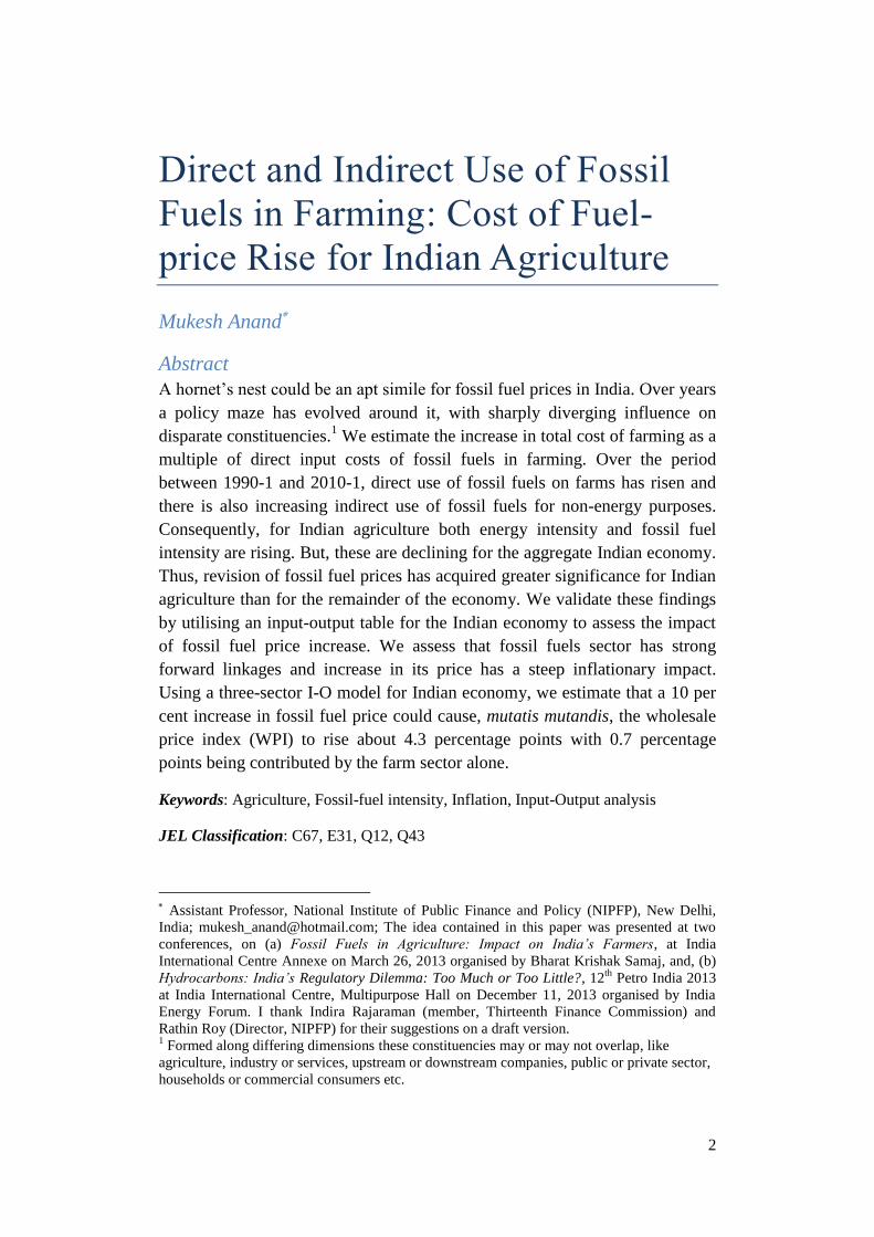
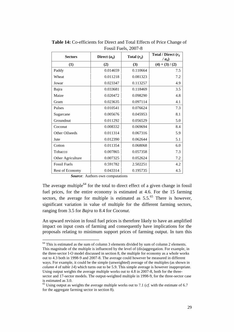
Table 14: Co-efficients for Direct and Total Effects of Price Change of

Fossil Fuels, 2007-8

Sectors Direct (aij) Total (rij) Total / Direct (rij

/ aij)

(1) (2) (3) (4) = (3) / (2)

Paddy 0.014659 0.110664 7.5

Wheat 0.011218 0.081323 7.2

Jowar 0.023347 0.113257 4.9

Bajra 0.033681 0.118469 3.5

Maize 0.020472 0.098290 4.8

Gram 0.023635 0.097114 4.1

Pulses 0.010541 0.076624 7.3

Sugarcane 0.005676 0.045953 8.1

Groundnut 0.011292 0.056529 5.0

Coconut 0.008332 0.069694 8.4

Other Oilseeds 0.011314 0.067316 5.9

Jute 0.012390 0.062644 5.1

Cotton 0.011354 0.068068 6.0

Tobacco 0.007865 0.057358 7.3

Other Agriculture 0.007325 0.052624 7.2

Fossil Fuels 0.591782 2.502251 4.2

Rest of Economy 0.043314 0.195735 4.5

Source: Authors own computations

The average multiple64

for the total to direct effect of a given change in fossil

fuel prices, for the entire economy is estimated at 4.6. For the 15 farming

sectors, the average for multiple is estimated as 5.5.65

There is however,

significant variation in value of multiple for the different farming sectors,

ranging from 3.5 for Bajra to 8.4 for Coconut.

An upward revision in fossil fuel prices is therefore likely to have an amplified

impact on input costs of farming and consequently have implications for the

proposals relating to minimum support prices of farming output. In turn this

64

This is estimated as the sum of column 3 elements divided by sum of column 2 elements.

This magnitude of the multiple is influenced by the level of (dis)aggregation. For example, in

the three-sector I-O model discussed in section 8, the multiple for economy as a whole works

out to 4.3 both in 1998-9 and 2007-8. The average could however be measured in different

ways. For example, it could be the simple (unweighted) average of the multiples (as shown in

column 4 of table 14) which turns out to be 5.9. This simple average is however inappropriate.

Using output weights the average multiple works out to 4.8 in 2007-8, both for the three-

sector and 17-sector models. The output-weighted multiple in 1998-9, for the three-sector case

is estimated as 3.0. 65

Using output as weights the average multiple works out to 7.1 (cf. with the estimate of 6.7

for the aggregate farming sector in section 8).

30

would influence the costs relating to the policy on food security and food

subsidy. This is however, beyond the scope of extant analysis.

10. Summary and conclusions

Inadequacy of extant evidence on the likely economic impact of an upward

revision in fossil fuel prices has emboldened a strong political opposition (or

fostered only a weak constituency). Utilising economy-wide linkages based on

input-output tables for the Indian economy, this paper musters some evidence

that the perception of strong adverse (inflationary) impact may not be

unfounded.

Production technology choices are shaped by the macro and micro policies. It

appears that the extant policy environment has intensified fossil fuel use, but

relatively more sharply in case of agriculture. This is likely to have continued

relevance for maintaining balance in the cross-subsidising scheme of pricing

fossil fuels.

Fossil fuels have strong forward linkages with the power and fertiliser sectors.

Increase in fossil fuel prices is likely to have strong implications for

continuing with the extant policies on fertiliser and power subsidies. These are

likely to aggravate the propagation of stress on public resources.

An increase of (say) 10 per cent in fossil fuel prices that may raise direct input

cost of farming, on an average by 0.56 per cent (table 7, section 4), could

impact total farming costs by about 3.75 (= 6.7 * 0.56) per cent. In turn, this

alone could add 0.70 percentage points to WPI based inflation. Estimates from

a three-sector model for the Indian economy suggest that the increase in WPI

based inflation could exceed 4.3 percentage points (cf. footnote 64).

Thus, rise in fossil fuel prices could manifest in higher inflation in farm-output

prices than what is normally portrayed in the literature. The cost-push effect

may be aggravated by the existence of demand-pull factors from growth in

incomes. It is likely to raise the cost of implementing the policy on food

subsidy and food security.

It is only appropriate to add a caveat that this is essentially a static exercise

based on input-output coefficients. Between 1998-9 and 2007-8, the forward

linkage of fossil fuels with the remainder of Indian economy has aggravated.

But, it could also weaken in future. Technological forecasting to enable such

analysis is far beyond the scope of this paper.

31

References

Anand M. K. (2012), Diesel Pricing in India: Entangled in Policy Maze,

National Institute of Public Finance and Policy, WP No. 2012-108, pg 41,

October 2012. http://www.nipfp.org.in/newweb/sites/default/files/WP_2012_108.pdf

Bandara, Jayatilleke S. (2013), What Is Driving India's Food Inflation? A

Survey of Recent Evidence, South Asia Economic Journal, March 2013,

14(1);127-56.

Bhanumurthy N. R., Surajit Das and Sukanya Bose (2012), Oil Price Shock,

Pass-through Policy and its Impact on India, NIPFP, Working Paper No.

2012-99, March 2012.

Bhattacharya, B.B. and A. Batra (2009). Fuel pricing policy reform in India:

Implications and Way Forward, Economic and Political Weekly, 49 (29).

Bhattacharya, Kaushik and Indranil Bhattacharyya (2001) Impact of Increase

in Oil Prices on Inflation and Output in India, Economic and Political

Weekly, 36(51);4735-4741 (Dec. 22-28).

Bulmer-Thomas V (1982), Input-Output Analysis in Developing Countries:

Sources, Methods and Applications, John Wiley and Sons Ltd, New York.

Centre for Monitoring Indian Economy (CMIE), 2013.

http://economicoutlook.cmie.com/kommon/bin/sr.php?kall=wshreport&&

repcode=016017015010010010000000000000000000000000000&repnu

m=12932&prs=000-999-999-00012930 Accessed on July 1, 2013.

Ganguly, Kavery, and Gulati, Ashok (2013), The political economy of food

price policy: The case study of India, pp. 28, World Institute for

Development Economic Research (UNU-WIDER), Working Papers:

UNU-WIDER Research Paper WP2013/034.

GoI (2006), Report of the Committee on Pricing and Taxation of Petroleum

Products, Chairman Dr. C. Rangarajan, February 2006.

GoI (2010), Report of the Expert Group on A Viable and Sustainable System

of Pricing of Petroleum Products, Chairman Dr. Kirit Parikh, February

2010.

http://web.ebscohost.com/ehost/viewarticle?data=dGJyMPPp44rp2%2fdV0%2bnjisfk5Ie45PFIrqeuUbWk63nn5Kx95uXxjL6nrUqxpbBIr6qeSbCwrlC4qa84v8OkjPDX7Ivf2fKB7eTnfLuttk62rbBOtKqkhN%2fk5VXj5KR84LPje%2byc8nnls79mpNfsVa%2bpt0i3q68%2b5OXwhd%2fqu37z4uqM4%2b7y&hid=4112

http://web.ebscohost.com/ehost/viewarticle?data=dGJyMPPp44rp2%2fdV0%2bnjisfk5Ie45PFIrqeuUbWk63nn5Kx95uXxjL6nrUqxpbBIr6qeSbCwrlC4qa84v8OkjPDX7Ivf2fKB7eTnfLuttk62rbBOtKqkhN%2fk5VXj5KR84LPje%2byc8nnls79mpNfsVa%2bpt0i3q68%2b5OXwhd%2fqu37z4uqM4%2b7y&hid=4112

http://economicoutlook.cmie.com/kommon/bin/sr.php?kall=wshreport&&repcode=016017015010010010000000000000000000000000000&repnum=12932&prs=000-999-999-00012930



http://web.ebscohost.com/ehost/viewarticle?data=dGJyMPPp44rp2%2fdV0%2bnjisfk5Ie45PFIrqeuUbWk63nn5Kx95uXxjL6nrUqxpbBIr6qeSbCwrlC4qa84v8OkjPDX7Ivf2fKB7eTnfLuttk62rbBOtKqkhN%2fk5VXj5KR84LPje%2byc8nnls79mpNfsVa%2bptVCxrLI%2b5OXwhd%2fqu37z4uqM4%2b7y&hid=4112

http://web.ebscohost.com/ehost/viewarticle?data=dGJyMPPp44rp2%2fdV0%2bnjisfk5Ie45PFIrqeuUbWk63nn5Kx95uXxjL6nrUqxpbBIr6qeSbCwrlC4qa84v8OkjPDX7Ivf2fKB7eTnfLuttk62rbBOtKqkhN%2fk5VXj5KR84LPje%2byc8nnls79mpNfsVa%2bptVCxrLI%2b5OXwhd%2fqu37z4uqM4%2b7y&hid=4112

32

GoI (2012), Basic Statistics on Indian Petroleum & Natural Gas, 2011-2,

Economic Division, Ministry of Petroleum & Natural Gas, Government of

India, New Delhi, September 2012.

GoI (2013), Energy Statistics, 2013 (Twentieth Issue), CSO, MoSPI, GoI,

New Delhi.

GoI (2013), Report of the Expert Group to Advise on Pricing Methodology of

Diesel, Domestic LPG, and PDS Kerosene, Chairman Dr. Kirit Parikh,

October 2013.

GoI (2013), Indian Petroleum and Natural Gas Statistics 2011-2, Economic

Division, Ministry of Petroleum and Natural Gas, Government of India,

New Delhi, January 2013.

http://mospi.nic.in/Mospi_New/upload/Energy_Statistics_2013.pdf

http://mospi.nic.in/Mospi_New/upload/NAS13.htm; Accessed on April 16,

2013

http://petroleum.nic.in/pngstat.pdf; Accessed on April 16, 2013

http://www.cseindia.org/dte-supplement/air20040331/dieselised.htm

http://www.iea.org/statistics/statisticssearch/report/?country=INDIA&product

=balances&year=1990


=balances&year=1998


=balances&year=2001


=balances&year=2007


=balances&year=2011

RBI (2011), Price Situation, Reserve Bank of India Monthly Bulletin, May

2011, pp 636-45.

RBI (2011a), The Challenge of Food Inflation, Presidential Address delivered

by Dr. Duvvuri Subbarao, Governor, Reserve Bank of India at the 25th



http://www.cseindia.org/dte-supplement/air20040331/dieselised.htm



33

Annual Conference of the Indian Society of Agricultural Marketing at

Hyderabad on November 22, 2011.

http://www.rbi.org.in/scripts/BS_SpeechesView.aspx?Id=630; Accessed

on January 27, 2014.

RBI (2011b), Food Inflation: This Time it's Different*, Kale Memorial

Lecture delivered by Dr. Subir Gokarn, Deputy Governor, Reserve Bank

of India at the Gokhale Institute of Politics and Economics, Pune on

December 9, 2011.



RBI (2014), Why is Recent Food Inflation in India so Persistent? Speech

delivered by Deepak Mohanty, Executive Director, Reserve Bank of

India, at the St. Xavier’s College, Mumbai on 13th January 2014.



TERI (The Energy and Resources Institute), 2012. The Energy Data Directory and

Yearbook (TEDDY), 2011/12, New Delhi: TERI.

http://www.rbi.org.in/scripts/BS_SpeechesView.aspx?Id=630

http://www.rbi.org.in/scripts/BS_SpeechesView.aspx?Id=638#st



34

Appendix

Table A:Operational Cost of Machine Labour for Different Crops, Maximum

of Average and Median for Reporting Provinces (in Per Cent of Total Cost

of Production per Hectare)

Crop Year Number

of States

Operational Cost of Machine Labour (per

cent)

Min. Max. Avg. Med. Max. of

6 & 7

1 2 3 4 5 6 7 8

Sugarcane 2010-1 7 1.0 8.7 3.0 2.2 3.0

1998-9 5 2.2 10.2 7.1 7.1 7.1

Wheat 2010-1 13 5.3 15.1 12.1 13.5 13.5

1998-9 6 7.0 11.2 9.7 10.5 10.5

Barley 2010-1 2 12.5 13.0 12.8 12.8 12.8

1998-9 2 10.3 10.8 10.6 10.6 10.6

Gram 2010-1 10 6.2 15.2 11.0 10.8 11.0

1999-00 4 4.7 12.1 8.7 9.1 9.1

Lentil 2010-1 5 3.5 19.7 10.7 10.9 10.9

1998-9 2 7.5 9.9 8.7 8.7 8.7

Rapeseed

& Mustard 2010-1 8 2.6 13.4 9.3 10.4 10.4

1998-9 6 0.2 14.8 10.1 11.1 11.1

Safflower 2010-1 2 0.2 6.8 3.5 3.5 3.5

1998-9 1 1.1 1.1 1.1 1.1 1.1

Paddy 2009-10 18 2.8 15.8 8.4 8.5 8.5

1998-9 9 1.0 11.3 5.1 5.1 5.1

Cotton 2009-10 10 1.5 8.4 4.6 4.6 4.6

1998-9 4 4.6 9.4 6.6 6.2 6.6

Jowar 2009-10 6 6.0 15.8 9.8 8.5 9.8

1998-9 4 2.4 11.8 5.4 3.7 5.4

Bajra 2009-10 6 7.8 13.0 10.9 10.9 10.9

1998-9 4 3.2 12.7 7.4 6.9 7.4

Maize 2009-10 10 0.0 12.5 7.6 7.7 7.7

1998-9 5 1.5 6.4 3.4 2.8 3.4

Ragi 2009-10 4 0.5 6.2 2.2 1.0 2.2

1998-9 3 0.0 4.1 1.9 1.6 1.9

Tur

(Arhar) 2009-10 9 0.9 10.5 7.0 7.0 7.0

1998-9 6 0.0 5.0 3.0 3.5 3.5

Moong 2009-10 5 1.1 14.9 8.1 10.5 10.5

1998-9 3 0.7 5.3 3.1 3.2 3.2

Urad 2009-10 8 1.0 21.1 10.7 9.8 10.7

1998-9 3 0.0 6.3 3.6 4.6 4.6

35

Crop Year Number

of States

Operational Cost of Machine Labour (per

cent)

Min. Max. Avg. Med. Max. of

6 & 7

1 2 3 4 5 6 7 8

Groundnut 2009-10 6 2.8 6.9 4.6 4.2 4.6

1998-9 3 0.1 4.5 2.0 1.8 2.0

Soyabean 2009-10 3 9.8 13.5 11.7 11.8 11.8

1998-9 3 4.9 11.1 8.3 8.8 8.8

Sunflower 2009-10 3 6.3 8.5 7.4 7.2 7.4

1998-9 3 3.2 7.2 4.9 4.4 4.9

Sesamum 2009-10 5 1.8 8.5 5.7 6.3 6.3

1998-9 5 0.0 7.2 3.7 3.9 3.9

Nigerseed 2009-10 1 3.7 3.7 3.7 3.7 3.7

1998-9 1 0.0 0.0 0.0 0.0 0.0

Jute 2009-10 3 0.4 3.1 1.9 2.2 2.2

1998-9 3 1.1 2.5 1.9 2.0 2.0

VFC

Tobacco 2008-9 1 19.1 19.1 19.1 19.1 19.1

1998-9 1 18.8 18.8 18.8 18.8 18.8

Documents

Direct and Indirect use of Fossil Fuels in Farming: Cost of … 1. Introduction This paper focusses on the interaction between fossil fuels and farming in India, to capture total intensity