Direct 2D simulation of small gas bubble clusters: from ...bruchon/articles/bruchon_fortin.pdf · 1 GIREF, D¶epartement de math¶ematiques et de statistique, Universit¶e Laval,

INTERNATIONAL JOURNAL FOR NUMERICAL METHODS IN FLUIDS

Int. J. Numer. Meth. Fluids 2006; 00:1–29 Prepared using fldauth.cls [Version: 2002/09/18 v1.01]

Direct 2D simulation of small gas bubble clusters: from theexpansion step to the equilibrium state

J. Bruchon1, A. Fortin1,∗ M. Bousmina2, K. Benmoussa1

1 GIREF, Departement de mathematiques et de statistique, Universite Laval, Quebec, Canada, G1K 7P42 Departement de genie chimique Universite Laval, Quebec, Canada, G1K 7P4

SUMMARY

A numerical strategy, based on an adaptive finite element method, is proposed for the direct two-

dimensional simulation of the expansion of small clusters of gas bubbles within a Newtonian liquid

matrix. The velocity and pressure fields in the liquid are first defined through the Stokes equations

and are subsequently extended to the gas bubbles. The liquid-gas coupling is imposed through the

stress exerted on the liquid by gas pressure (ruled by an ideal gas law) and by surface tension. A

level set method, combined with a mesh adaptation technique, is used to track liquid-gas interfaces.

Many numerical simulations are presented. The single bubble case allows to compare the simulations

to an analytical model. Simulations of the expansion of small clusters are then presented showing

the interaction and evolution of the gas bubbles to an equilibrium state, involving topological

rearrangements induced by Plateau’s rule. Copyright c© 2006 John Wiley & Sons, Ltd.

key words: Level set method, Mesh adaptation method, Liquid-gas coupling, Gas bubble cluster

expansion, Laplace’s rule, Plateau’s rule

∗Correspondence to: GIREF, Departement de mathematiques et de statistique, Universite Laval, Quebec,Canada, G1K 7P4

Contract/grant sponsor: NSERC

Received February 2006

Copyright c© 2006 John Wiley & Sons, Ltd. Revised

2 J. BRUCHON, A. FORTIN, M. BOUSMINA, K. BENMOUSSA

1. INTRODUCTION

The study of gas bubbles embedded into a liquid matrix is of great theoretical and industrial

interest, at the crossroads of engineering, physics and mathematics [1, 21]. The equilibrium

configuration of a bubble cluster is governed by surface tension through two laws: Laplace’s

law, which relates the curvature of the interface to the pressure difference inside and outside;

Plateau’s rule, which states that bubbles can meet only in groups of three, at angles of 120.

This last rule implies a minimal surface area property, leading to instabilities and topological

rearrangements into larger clusters. In the literature, such situations are investigated in the

framework of liquid foams (see [20, 10, 19]). Usual approaches for modeling and simulating

these phenomena are essentially based on minimal surface area criteria (see [15, 6]).

The present paper proposes a direct simulation, using a finite element method, of the

evolution of a set of bubbles into a Newtonian fluid. The first difficulty of this approach

is the liquid-gas coupling: the gas is a compressible fluid, having an inner pressure ruled by the

ideal gas law, and exerting a stress on the liquid matrix. When the pressure is not balanced

by surface tension forces (equilibrium is not yet reached), this stress allows for the expansion

of the gas (see [8]). The second difficulty is to obtain a good description of the interfaces:

bubbles interact between themselves and can adopt a wide variety of shapes. Furthermore,

the interfaces come very close to each other during the process. Consequently, if the numerical

method is not accurate enough, numerical diffusion can provoke a purely artificial (numerical)

coalescence of bubbles (see Fortin and Benmoussa [14]). The interface tracking method used

in the present work is the level set method coupled with an adaptive remeshing strategy which

is more completely described in Fortin and Benmoussa in [13].

The first section of this paper is devoted to the mathematical description of the expansion

Copyright c© 2006 John Wiley & Sons, Ltd. Int. J. Numer. Meth. Fluids 2006; 00:1–29

Prepared using fldauth.cls

DIRECT 2D SIMULATION OF SMALL GAS BUBBLE CLUSTERS 3

of a bubble cluster into a liquid matrix, and to its finite element discretization. In the second

section, the expansion of a single bubble is studied. The simulations are compared to an

analytical model when neglecting surface tension, and to the Laplace’s law otherwise. The

third section investigates the expansion of several bubbles: cases with three, four and nine

bubbles allow for the comparison between simulations and real cluster configurations.

2. MATHEMATICAL FORMULATION

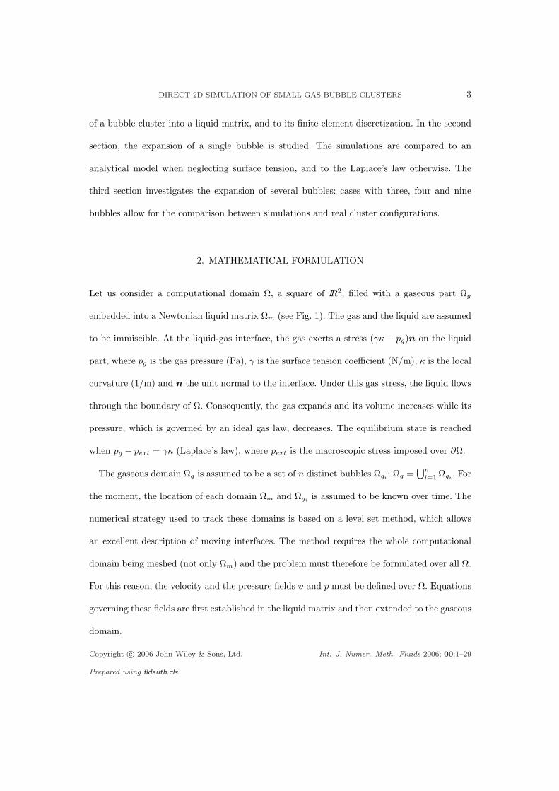
Let us consider a computational domain Ω, a square of IR2, filled with a gaseous part Ωg

embedded into a Newtonian liquid matrix Ωm (see Fig. 1). The gas and the liquid are assumed

to be immiscible. At the liquid-gas interface, the gas exerts a stress (γκ− pg)n on the liquid

part, where pg is the gas pressure (Pa), γ is the surface tension coefficient (N/m), κ is the local

curvature (1/m) and n the unit normal to the interface. Under this gas stress, the liquid flows

through the boundary of Ω. Consequently, the gas expands and its volume increases while its

pressure, which is governed by an ideal gas law, decreases. The equilibrium state is reached

when pg − pext = γκ (Laplace’s law), where pext is the macroscopic stress imposed over ∂Ω.

The gaseous domain Ωg is assumed to be a set of n distinct bubbles Ωgi : Ωg =⋃n

i=1 Ωgi . For

the moment, the location of each domain Ωm and Ωgi is assumed to be known over time. The

numerical strategy used to track these domains is based on a level set method, which allows

an excellent description of moving interfaces. The method requires the whole computational

domain being meshed (not only Ωm) and the problem must therefore be formulated over all Ω.

For this reason, the velocity and the pressure fields v and p must be defined over Ω. Equations

governing these fields are first established in the liquid matrix and then extended to the gaseous

domain.




2.1. Conservation and equilibrium equations in the liquid domain

In this work, the liquid matrix is assumed to be an incompressible Newtonian fluid in order

to focus only on surface tension effects and on liquid-gas coupling. The described numerical

method is however general and has been implemented in order to work equally well with shear-

thinning fluids governed by power or Carreau laws relating the liquid viscosity to the norm of

the strain rate tensor.

The Cauchy stress tensor σ in the fluid matrix is defined by σ = 2ηmε(v) − pI, where ηm

is the matrix viscosity. Influence of inertia can be evaluated through the Reynolds number

Re, which is obtained by balancing the inertia term with the viscosity term in the momentum

equation. Re can be defined by (see [12]):

Re =ρV

2/30 (p0

g − pext)η2

m

(1)

where ρ is the matrix density, V0 the initial bubble volume and p0g the initial gas

pressure. Following literature (see [16]), inertia is negligible in typical real 2D foam systems.

Consequently, inertia effects are neglected in the present paper and momentum and mass

conservation laws lead to the Stokes equations governing v and p:

∇ · [2ηmε(v)]−∇p = 0 in Ωm

∇ · v = 0 in Ωm

σn = (γκI + σgi)n on ∂Ωm ∩ ∂Ωgi

σn = −pextn on ∂Ωm ∩ ∂Ω

(2)

where σgi is the Cauchy stress tensor of the ith gas bubble.




2.2. Conservation and equilibrium equations in a gas bubble

The pressure pi in the bubble Ωgi and its volume |Ωgi | are governed by an ideal gas law which,

at constant temperature, gives:

pgi|Ωgi

| = constanti (3)

In this quasi-static model, the gas pressure is uniform in each bubble. Equation (3) does

not allow to describe the velocity field in the gas. However, the evolution of the volume of a

bubble depends only on the interface velocity. Hence, the velocity field already defined in Ωm,

is extended to Ωg in a way that does not perturb the interfacial velocity:

v ∈ C1(Ω)

∇ · [2ηgε(v)] = 0 in Ωg

(4)

where ηg is a (small) numerical parameter. Such an extension corresponds to the addition of a

viscosity term to the gas bubble Cauchy stress tensor: σgi = 2ηgε(v)−pgiI. In order to ensure

the consistency of the model, the parameter ηg must be chosen small enough so that:

2ηg‖ε(v)n‖IR2 ¿ pgi‖n‖IR2 = pgi (5)

on ∂Ωgi . Finally, the pressure field, already defined in Ωm, has also to be extended to Ωgi . A

natural extension is to set the pressure field p equal to the gas pressure into each bubble as in

Caboussat, Picasso and Rappaz [9]:

p = pgi in Ωgi (6)




However, the Cauchy stress tensor σgi is not related to the pressure field p, but is directly a

function of pgi, the bubble pressure. Hence, the value of p in Ωgi

does not appear in Eqs. (2),

and, consequently, can be chosen arbitrarily. This is why, in order to limit the perturbation of

the velocity and pressure fields already defined in Ωm, p is extended by zero in Ωg:

p = 0 in Ωg (7)

2.3. Velocity-pressure mixed variational formulation

Let us define the functional spaces V = (H1(Ω))2 and P = L2(Ω). The global mixed

formulation is obtained by adding the variational forms of (2), (4) and (7). The weak form of

(2) in the liquid domain is straightforward:

∫

Ωm

2ηmε(v) : ε(w)−∫

Ωm

p∇ ·w = −∫

∂Ω

pextn ·w

−∫

∂Ωg

γκn ·w −n∑

i=1

∫

∂Ωgi

σgin ·w∫

Ωm

q∇ · v = 0

(8)

∀(w, q) ∈ V × P. A similar formulation can be obtained in the gaseous part of the domain

from Eqs. (4) and (7):

∫

Ωg

2ηgε(v) : ε(w) =n∑

i=1

∫

∂Ωgi

(σgin + pgin) ·w∫

Ωg

p q = 0(9)

∀(w, q) ∈ V×P. In order to avoid dealing with surface integrals, these latter have to be turned

into volume integrals. The divergence theorem can directly be applied to the surface integral

involving the gas pressure. The surface tension term can be rewritten as a volumetric force as




in Brackbill et al. [5] and Beliveau et al. [4]. Assuming the interface ∂Ωg is smooth enough,

the following relation takes place in a distributional sense:

∇F = nδ∂Ωg (10)

where δ∂Ωg is the Dirac distribution associated to ∂Ωg and F , the characteristic function of

Ωg, is equal to 1 in Ωg and vanishes in Ωm. Relation (10) allows writing:

∫

∂Ωg

γκn ·w =∫

Ω

γκ∇F ·w (11)

To avoid the explicit computation of the local curvature κ, the following equality, proved in

[4] is considered:

∫

Ω

γκ∇F ·w =∫

Ω

γ

(∇F ⊗∇F − |∇F |2I|∇F |

): ∇w =:

∫

Ω

γT : ∇w (12)

The second order tensor γT will impose surface tension forces at the boundary of each gas

bubble. By adding Systems (8) and (9) and by taking into account relations (11) and (12), the

final mixed system is:




Find (v, p) ∈ V × P such that:

∫

Ωm

2ηmε(v) : ε(w) +∫

Ωg

2ηgε(v) : ε(w)−∫

Ωm

p∇ ·w =

−∫

∂Ω

pextw · n−∫

Ω

γT : ∇w +∫

Ω

pg∇ ·w

−∫

Ωm

q∇ · v − αp

∫

Ωg

p q = 0

∀(w, q) ∈ V × P

(13)

where the gas pressure pg equals pgi in Ωgi and vanishes in the liquid matrix Ωm and αp is

a numerical parameter, which allows to add the last equations of Systems (8) and (9), and

has the dimensions of the inverse of a viscosity. In the continuous case (13), Ωm ∩Ωg = ∅ and

the parameter αp is then arbitrary. However, in the discrete case, for a same given node, the

contributions to the mass matrix can be provided by both liquid and gaseous terms and αp

appears therefore as a weighting parameter. More precisely, it has to be chosen small enough

to ensure mass conservation in the liquid domain (αp = 10−5 in the presented simulations).

Before discussing the finite element implementation used for solving System (13), some

important points have to be outlined:

• The uniqueness of the solution of (13) is ensured by considering Dirichlet conditions for

the velocity v over a part of the boundary ∂Ω. These conditions will be defined in the

following for each considered case.

• The gas pressure field involved in (13) is calculated with n relations of the form (3). The

simulations require the volume of each bubble, and need a special treatment (see section

4).




• By construction, the velocity and the pressure fields (v, p) solution of (2), (4) and (7),

are also a solution of the weak mixed formulation (13). In turn, if v and p are solution

of (13), and if the gas boundary is smooth enough, then v and p are also solution of (2),

(4) and (7) (in a distributional sense) and satisfy the boundary and interface conditions

considered in (2).

In order to use a finite element method for solving System (13), the integrals defined over

Ωm and Ωgihave to be turned into integrals defined over Ω. Such an operation is performed

by considering the characteristic function F of the gaseous domain, and its complementary

function 1−F . Multiplying the integrand by F (or (1−F )) will restrict the integral to Ωg (or

Ωm):

∫

Ωg

fdΩ =∫

Ω

FfdΩ,

∫

Ωm

fdΩ =∫

Ω

(1− F )fdΩ.

The second order (O(h2)) Taylor-Hood finite element (quadratic velocity and linear

pressure) is then used to discretize the resulting mixed formulation. Finally, the finite element

implementation is achieved by computing the characteristic function F of the gaseous part

i.e., by computing the evolution of the bubble position over time.

2.4. Interface capturing

The methodology used to capture the interfaces is described in details in [13] and is based on

a finite element approach and a level set method. Let us consider a function φ : Ω× IR+ → IR

describing the gaseous domain Ωg. Since Ωg is convected by the velocity field v, φ is solution

of a pure advection equation [17]:




∂φ

∂t+ v · ∇φ = 0 ∀t > 0

φ(. , 0) = φ0 at t = 0(14)

Solving such a hyperbolic equation is a difficult numerical task [7], and may involve spurious

oscillations when using standard finite elements. The level set method, developed in [17], avoids

the development of steep gradients by convecting a smooth function φ. More precisely, φ is

the signed distance function to the interface ∂Ωg, which is positive into Ωg, vanishes over ∂Ωg

and is negative in Ωm. Using this approach, φ ∈ C1(Ω) and ‖∇φ‖IR2 = 1. Equation (14) can

then be solved by a classical SUPG method.

As in [13], the simulations presented in this paper have been performed by using such a

level set method, with quadratic polynomials for the space discretization of φ and an implicit

Euler scheme for the time derivative. Note that even though φ0 is initially a signed distance

function, the solution φ of Equation (14) does not generally conserve this property. Hence, steep

gradients may progressively appear near the interface which becomes irregular. Consequently,

after solving Equation (14), an additional re-initialization step is necessary, which consists in

modifying the solution for obtaining ‖∇φ‖IR2 = 1, without changing the isovalue zero, i.e.,

without perturbing the interface position (see Sussman and Fatemi [18]).

When solving a hyperbolic equation like (14), boundary conditions have to be imposed only

over the inflow part of the boundary ∂Ω. Since the velocity field v involved in (14) is the

expansion velocity field, solution of (13), ∂Ω is usually an outflow boundary. Consequently,

function φ does not verify any boundary condition.

In the discrete case, the gas characteristic function F has to be smoothed out and is thus

defined by:




F =

0 if φ ≥ ε

12 (1− φ

ε − 1π sin(π φ

ε )) if |φ| ≤ ε

1 if φ ≤ −ε

(15)

where ε is a regularization parameter. Hence, the effective computed interface has a width of

2ε. This smooth form of F allows to consider its gradient, which is used to express the surface

tension tensor T in relation (12): ∇F = dFdφ∇φ.

To improve the accuracy on the interface location, a mesh adaptation method is used (see

[2, 3]). This method is based on a hierarchical error estimator. It concentrates the mesh

elements in the vicinity of the interfaces and allows to chose very small values of ε and thus

very thin interfaces. Hence, a good description of the interfaces is obtained with an acceptable

number of mesh elements.

2.5. Units used in the simulations

Simulation results considered here are given in a dimensionless form. More precisely, let x be the

characteristic length of the computational domain, and let p be the characteristic pressure.

The corresponding characteristic time is t = ηm/p, the characteristic velocity is defined by

v = x/t.

Let us consider the following decompositions: x = x∗x, y = y∗y, t = t∗t, p = p∗p, v = v∗v,

γ = γ∗p × x where x∗, y∗, t∗, p∗, v∗ and γ∗ are dimensionless numbers. For instance, by

considering ηm = 1Pa.s, x = 10−2 m and p = 102 Pa, then t = 10−2 s, v = 1 m/s and γ = 1

N/m.

System (13) has been solved by using the dimensionless quantities. Hence, whatever the

physical quantity q considered here, it is always its dimensionless part q∗ which is given. The




physical value of q is then equal to q∗q.

3. DIRECT SIMULATION OF SINGLE BUBBLE EXPANSION

In this rather simple case, an analytical model is developed for the expansion of a single bubble.

This model provides an analytical expression for the radius of a circular gas bubble growing

into an infinite Newtonian matrix, when neglecting surface tension. Comparisons between this

theoretical model and our simulation will thus be possible allowing to test the efficiency of the

presented approach. Surface tension will then be introduced and its effect on the expansion

will be tested.

3.1. Analytical model

Let us consider the growth of a disk of radius R(t), within an infinite matrix of a Newtonian

liquid. Cylindrical coordinates (r, θ) are used with the origin O chosen at the bubble center.

The kinematics of the liquid matrix are ideally described by a purely radial velocity field which

depends, as the pressure, only on the r-component: v = (u(r), 0), p = p(r). The initial bubble

radius is denoted by R(0) = R0, with a corresponding area V0 and a bubble pressure p0g. The

incompressibility condition of the liquid leads to:

1r

d

dr(ru) = 0, r ≥ R (16)

The solution of this first order differential equation using the condition at the interface

u(R) = dR/dt = R leads to:

u(r) =RR

rr ≥ R (17)




Due to the radial symmetry, the momentum balance is described by one single scalar

equation:

dσrr

dr+

1r

(σrr − σθθ) = 0 (18)

which is completed with appropriate boundary conditions:

σrr(R) = −pg

σrr(+∞) = −pext

(19)

Considering expression (17), the strain rate tensor is of the form:

ε(v) =RR

r2

−1 0

0 1

(20)

and Eq. (18) becomes: dpdr = 0. Furthermore, Eqs. (19) and (20) imply that p(+∞) = pext.

The pressure is thus constant in the liquid:

p(r) = pext r > R (21)

Finally, by considering the first condition in Eq. (19) and the stress at r = R, the growth

velocity R can be expressed as:

R

R=

pg − pext

2ηm(22)

This analytical expression is very useful in order to understand the expansion of a bubble,

and the above results require some comments. First, note the absence of shear stress in (20).

Second, since the pressure is constant in the liquid matrix, the liquid-gas interface is a




discontinuity surface (or line in 2D) for the pressure but the normal stress is continuous

across this surface when surface tension is neglected. Furthermore, the local growth velocity,

expressed by Equation (22), depends only on the local pressure difference which corresponds

also to the global pressure difference.

In order to solve Equation (22), the gas pressure has to be related to the radius. Three cases

can be distinguished:

Constant gas pressure: pg(t) = p0g and

R(t) = R0 exp(

(pg − pext)t2ηm

)(23)

Ideal gas law: pgV = p0gV0, i.e. pg = p0

gR20/R2 and

if pext 6= 0, then:

R(t) = R0

[p0

g

pext+

(1− p0

g

pext

)exp

(−pextt

ηm

)]1/2

(24)

if pext = 0, then:

R(t) = R0

(1 +

p0gt

ηm

)1/2

(25)

3.2. Numerical results without surface tension

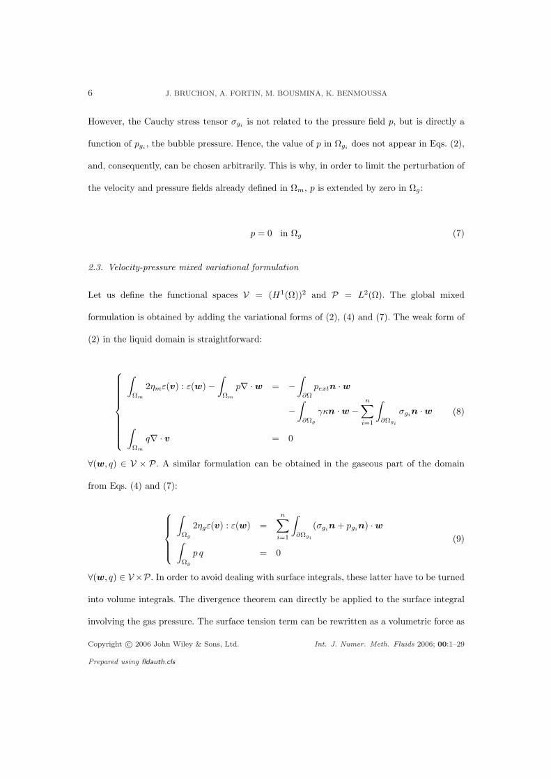
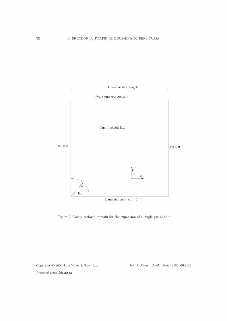
The presented simulations of the expansion of a single bubble have been performed in the

configuration shown in Figure 2. Symmetry considerations allow for considering only one

quarter of the bubble. Appropriate Dirichlet boundary conditions have therefore to be imposed

over symmetry axes: vx = 0 is enforced on x = 0, and vy = 0 on y = 0, with v = (vx, vy).

Surface tension is neglected (γ = 0) and the ambient pressure pext is taken equal to zero.




Hence, the bubble can grow indefinitely. The initial bubble pressure is p0g = 0.2, its initial

radius is R0 = 0.1, the matrix viscosity ηm is equal to 1, and the value of ηg is 10−3. These

parameters are expressed in the chosen units.

Regarding the ideal gas law (3), the bubble pressure is defined by: pb = p0gV0

|Ωg| , where

|Ωg| =∫

Ωg

1 dΩ =∫

φ<01 dΩ

The gas pressure field, involved in the mixed formulation (13) is then defined by: pg = pbF .

Figure 3 shows the liquid-gas interface superimposed on isovalues of the first component of

the computed velocity, at a fixed time. As expected, the obtained velocity field is characteristic

of an expansion. It reaches its maximal absolute values over the interface, because of the stress

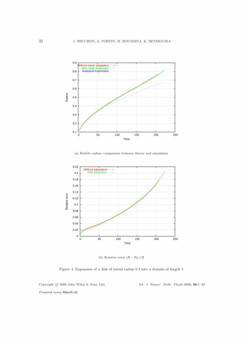
exerted by the gas. Figure 4(a) compares, over time, the radius Rh obtained by simulation

with the one calculated with the analytical expression (25). Figure 4(b) quantifies this study

by expressing the relative error committed on the radius: eh = |R − Rh|/R. Until t ' 50, the

agreement between simulations and theory is quite good, and the relative error is smaller than

4 %. Beyond this value, the error growth seems exponential. The change in the error occurs

when the bubble radius reaches one third of the computational domain length (here, Ω is the

unit square). These disappointing results are easily explained by boundary effects. Indeed, the

analytical model assumes that the expansion is taking place into an infinite domain, while

the computational domain is finite. This analysis is validated in Figure 5, which shows the

simulation results obtained by using a computational domain ten times larger than before. As

long as the radius is smaller than one third of the computational domain length, the agreement

between simulation and theory is excellent.

Finally, Figure 4 shows that mesh adaptation does not perturb the bubble’s expansion. The

mesh used to perform the simulations without adaptation has more than 20 000 elements, while




the different adapted meshes have between 2000 and 5000 elements. Furthermore, simulations

involving a computational domain having a characteristic length of 10, can be carried out

only by using mesh adaptation since the ratio between computational domain and bubble

characteristic lengths is equal to 100 and the number of mesh elements required without mesh

adaptation is too high.

3.3. Numerical results with surface tension

Expansion of a single bubble is simulated by considering the same configuration and the

same parameters as in section 3.2, except that surface tension is now taken into account. The

surface tension coefficient γ (from Equation (2)) is equal to 10−2. Since pext is still vanishing,

the bubble should grow until the gas pressure pb reaches γR . Considering the ideal gas law

pbR2 = p0

gR20, the corresponding equilibrium radius is:

Req =p0

gR20

γ(26)

Figure 6 presents the results of a simulation performed using a computational domain having

a characteristic length of 10. Since p0g = 0.2 and R0 = 0.1, the theoretical equilibrium radius

is Req = 0.2, and the associated equilibrium pressure is peq = 5 × 10−2. These equilibrium

values are exactly those reached by the simulation. The small oscillations observed in Figure

6 are due to the change in the time step, which increases over time.

4. DIRECT SIMULATION OF THE EXPANSION OF BUBBLE CLUSTERS

The previous simulations, involving only one bubble, have proved the accuracy of the

developed method for the liquid-gas coupling. They have also validated the approach for the




computation of the surface tension term. Dealing with a bubble cluster adds another degree

of complexity to the simulations. The bubbles will now interact between themselves and the

corresponding interfaces will get more complicated. Furthermore, due to surface tension effects,

the equilibrium configuration of a bubble cluster both satisfy Laplace’s law γκ = pg − pext

and Plateau’s rule [21]. This last one states, in a liquid foam framework, that bubbles meet

in cluster of three, forming angles of 120o. It has to be pointed out that the two different

parts composing Plateau’s rule are important. Firstly, ”clusters of three” means that the

configuration resulting from the meeting of four (or more) bubbles is unstable and leads to

topological changes to minimize the interfaces. Such events are depicted in Figure 7(a) for

the case involving four bubbles (see [11] and [15]). Secondly, the resulting angles of 120o (see

Figure 7(b)) are a simple consequence of the equilibrium of surface tension forces acting over

bubble surfaces. This subject will be detailed in the following.

Since the normal stress pext, enforced over the boundary of Ω, is constant, the pressure

within the liquid domain is constant and equal to pext (see paragraph 3.1). Hence, at the

equilibrium state, Laplace’s law states that for the ith bubble, pgi−γ/Ri = pext. But pgi being

uniform in the bubble, this relation implies that Ri is uniform and the bubble is spherical (or

circular) when reaching its equilibrium state.

To carry out simulations with several bubbles, it is necessary to avoid the ”numerical”

coalescence of two neighboring bubbles which can occur when the mesh is too coarse at the

interface between two bubbles. On a coarse mesh, the computation of the signed distance

function φ giving the interfaces position can suffer from excessive numerical diffusion leading

to an artificial coalescence of adjacent bubbles. Mesh adaptation plays a major role here. It

allows to concentrate the elements in a very narrow band of width 2ε along the interface.




In the following computations, ε is taken equal to 5 × 10−3, compared to an initial bubble

characteristic length of 0.1.

The computation of the bubble pressures is another key point of the cluster simulations.

From Equation (3), it is necessary to compute the volume of each bubble. If a signed distance

function φi is associated to each bubble Ωgi, the volume of this bubble is simply given by:

|Ωgi | =∫

φi<01 dΩ. The drawback of this approach is its computational cost since for n bubbles,

n distance functions have to be stored and n advection equations have to be solved. To avoid

this important cost, one single signed distance function φ is considered and an algorithm is

developed to rebuild the different bubble volumes.

4.1. Algorithm for bubble volume reconstruction

The liquid-gas coupling exposed in the present paper presents similarities with the one

developed in Caboussat, Picasso and Rappaz [9]. The algorithm proposed here is simpler: one

single loop over the mesh elements is necessary to number all the bubbles and to determine

their volumes. In [9], the numbering of the gas bubbles requires the solution of a Poisson

equation for each bubble. When the location of a bubble is identified, a loop over the mesh

elements enables to compute its volume.

Let EltV isited be a boolean array of length NbElt, the number of elements of the mesh

Th(Ω), whose values 0 or 1 correspond to the state of each element: not visited yet or already

visited. The aim of the algorithm is to construct BubbleTracker, an integer array, of length

NbElt, whose values indicate if an element belongs to the liquid (value 0), or to the ith bubble

(value i). Once this array exists, it is very easy to calculate the bubble volumes and the

pressure field pg involved in Equation (13). Hence, ∀K ∈ Th(Ω), ∀x ∈ K, pg |K(x) = F|K(x)pb,




where pb is the pressure of the bubble number BubbleTracker[K], computed by the ideal gas

law (3) (and pb = 0 if BubbleTracker[K] is equal to zero). This approach could be improved

by looking for the bubble number at quadrature points. However, the algorithm shows good

results without this improvement, which is not considered here. The algorithm is:

begin

integer i ← 0

boolean EltV isited[NbElt]

integer BubbleTracker[NbElt]

while (i < NbElt)

EltV isited[i] ← 0 \\ Initialization

BubbleTracker[i] ← 0

i ← i + 1

Integer NbBubbles ← 0 \\ The number of bubbles

i ← 0

while (i < NbElt)

if (EltV isited[i] == 0)

boolean GaseousElt = IsGas(i)

if (GaseousElt == 1) \\ New bubble

NbBubbles ← NbBubbles + 1

ExploreNewBubble(i,NbBubbles, EltV isited, BubbleTracker)

else EltV isited[i] ← 1




i ← i + 1

end

The function IsGas(i) evaluates the signed distance function φ over the mesh element i

and returns the value 1 if φ < 0 (the element is in the gas) and the value 0 otherwise.

The function ExploreNewBubble(i, NbBubbles, EltV isited, BubbleTracker) explores a new

bubble starting from the element i. More precisely, starting from i, this function constructs

a new bubble by adding gradually the neighbors of i, the neighbors of the neighbors, and

so on, while φ is found negative. For each element K added to the bubble, the function sets

EltV isited[K] = 1 and BubbleTracker[K] = NbBubbles.

Using this algorithm the number associated to a given bubble can vary from one time step

to the next. That is why an additional task is required to determine the number of the ith

bubble at the previous time step (and then to know what was its previous volume). Since

bubble coalescence or breakup is not allowed, each bubble is simply characterized through the

point X located inside this bubble minimizing φ. For example, the fact that X = (x, y) ∈ Ω1

at the time t1 and X ∈ Ω3 at the time t1 + ∆t, implies Ω1(t1) ≡ Ω3(t1 + ∆t), and then

p3(t1 + ∆t) =p1(t1)|Ω1(t1)||Ω3(t1 + ∆t)| .

4.2. Expansion of a three bubble cluster

The presented simulation has been carried out by taking pext = 0, p0gi|Ω0

gi| = 0.0314 and

R0i = R0 = 0.1, i = 1, 2, 3. The surface tension coefficient γ is equal to 10−2. Moreover, the




characteristic length of the computational domain is equal to 10. The initial bubble centers

are: (0.15,0), (-0.15,-0.05) and (0.03,0.25) (see Figure 8(a)). This initial configuration does not

respect the angles of 120o between the bubbles. To ensure the uniqueness of the solution of

system (13), Dirichlet boundary conditions must be considered: the velocity field is assumed to

vanish at the four corners of the squared computational domain. This condition is in agreement

with expression (17) of the velocity field: when being far enough from the bubbles, liquid

remains at rest. Furthermore, enforcing boundary conditions in the four corners of the domain

(and not only in one corner) avoid an additional dissymmetry in the system.

The complete evolution of the bubbles and the corresponding meshes are depicted in

Figures 8 and 9. By considering the form of the velocity field (Figures 10 and 12), the

expansion of the cluster depicted in Figure 8 can be divided into three different stages. Initially

(Figure 8(a)), bubbles have the same uniform curvature, equal to 1/R0. During the first stage

of the expansion (Figure 8(b)), bubbles interact between themselves, changing their shape and

then their local curvature. However, despite this local curvature change, the surface tension

term γκ has not a significative influence on the expansion. Hence, the velocity field plotted

in Figure 10(a) is similar to the one of an expansion without surface tension (see [8]). That

can be explained by two factors. The first one is the distance separating the bubble surfaces,

which is high enough to limit the effect of a curvature difference. The second factor is the small

contribution of the surface tension term (equal to 0.1 at t = 0) to the normal stress exerted

on the liquid, compared to the one of the gas pressure (equal to 1 at the beginning). However,

note that the gas pressure decreases as 1/R2, while the surface tension term decreases as 1/R.

During the second stage (Figures 8(c) and 8(d)), the bubble surfaces are close to each other

and the expansion is affected by the surface tension. Hence, during this period, the velocity




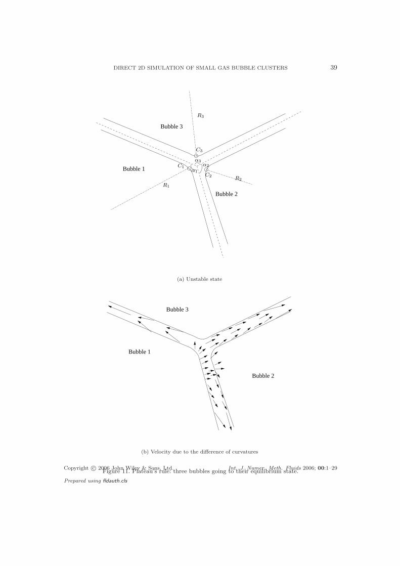
field (Figures 10(b) and 12(a)) shows a special orientation in the center of the cluster, due

to the differences between the local curvatures. For interpreting this velocity, let us consider

the Figure 11(a) describing the situation. First, by looking at Figure 13, note that the three

bubbles have approximatively the same volume, and then the same inner pressure pg, all along

their expansion. Since α1 > α2, 1/R1 < 1/R2, the norm |(pg − γ/R1)| of the normal stress

exerted by the bubble 1 on the liquid matrix, is higher than |pg−γ/R2|, the norm of the normal

stress induced by the bubble 2. Assuming α2 < α3 (as in the simulation), Figure 11(b) gives

a rough description of the velocity field resulting from the stress difference: bubble number 2

can not grow in the direction of bubbles number 1 and 3. Furthermore, such a velocity field

leads to a decrease of α1 and an increase of α2: this behavior is the one observed in Figure 8.

Finally, angles α1, α2 and α3 reach the value of 120, with a precision of more or less

three degrees (Figures 8(e) and 8(f)). This value appears to be an equilibrium value: since

the three bubbles have the same local curvature in the vicinity of the cluster center, their

relative positions do not evolve any more. Because the pressure in the matrix is uniform (and

equal to zero in the simulation), a bubble should reach a spherical shape at the equilibrium

(Laplace’s law). Hence, during the last period, the angles remain unchanged, but the bubbles

tend to recover a spherical shape. The bubble volume, plotted over the time in Figure 13

shows that the expansion stops at t = 600, approximately. The velocity field has the form

considered in Figure 12(b): the expansion is stopped, while small curvature differences provide

oscillations of the velocity into the cluster. Note that bubbles of Figure 8(f) have not reached

their equilibrium state yet. Their evolution toward the equilibrium proceeds very slowly.

To conclude, the evolution of the number of elements generated by the mesh adaptation is

plotted in Figure 14. This number is proportional to the length of the bubble boundary.




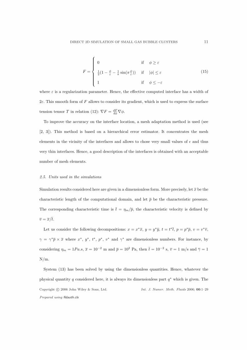
4.3. Expansion of a four bubble cluster

This simulation has been performed by considering: pext = 0, p0gi|Ω0

gi| = 0.2 and |Ωgi | ' 0.17,

i = 1, 2, 3, 4. The surface tension coefficient is γ = 2×10−2. The initial configuration, depicted

in Figures 15(a) and 17(b) is a pathological one: the bubbles are identical and are forming a

group of four meeting at angles of 90o. They are inscribed in a circle of radius 0.5, and spaced

by a distance of 0.05. As in previous case, the squared computational domain has a side length

of 10. The velocity field is forced to vanish in its four corners.

Figure 15 shows the expansion of the bubble cluster. Due to the closeness of the interfaces

in the initial configuration, the topological change depicted in Figure 7(a) occurs as soon as

the simulation starts (Figures 15(c) and 15(d)). The cluster reaches its stable configuration

at time t ' 100, forming two groups of three bubbles meeting at angles of 120o. During this

rearrangement, the bubble volumes become heterogeneous, as it can be seen in Figure 16.

Beyond t = 100, the bubbles continue to grow but remain in this stable configuration. At

t = 200, the two larger bubbles reach their equilibrium size: their expansion is stopped. The

two others evolve progressively toward this same equilibrium size.

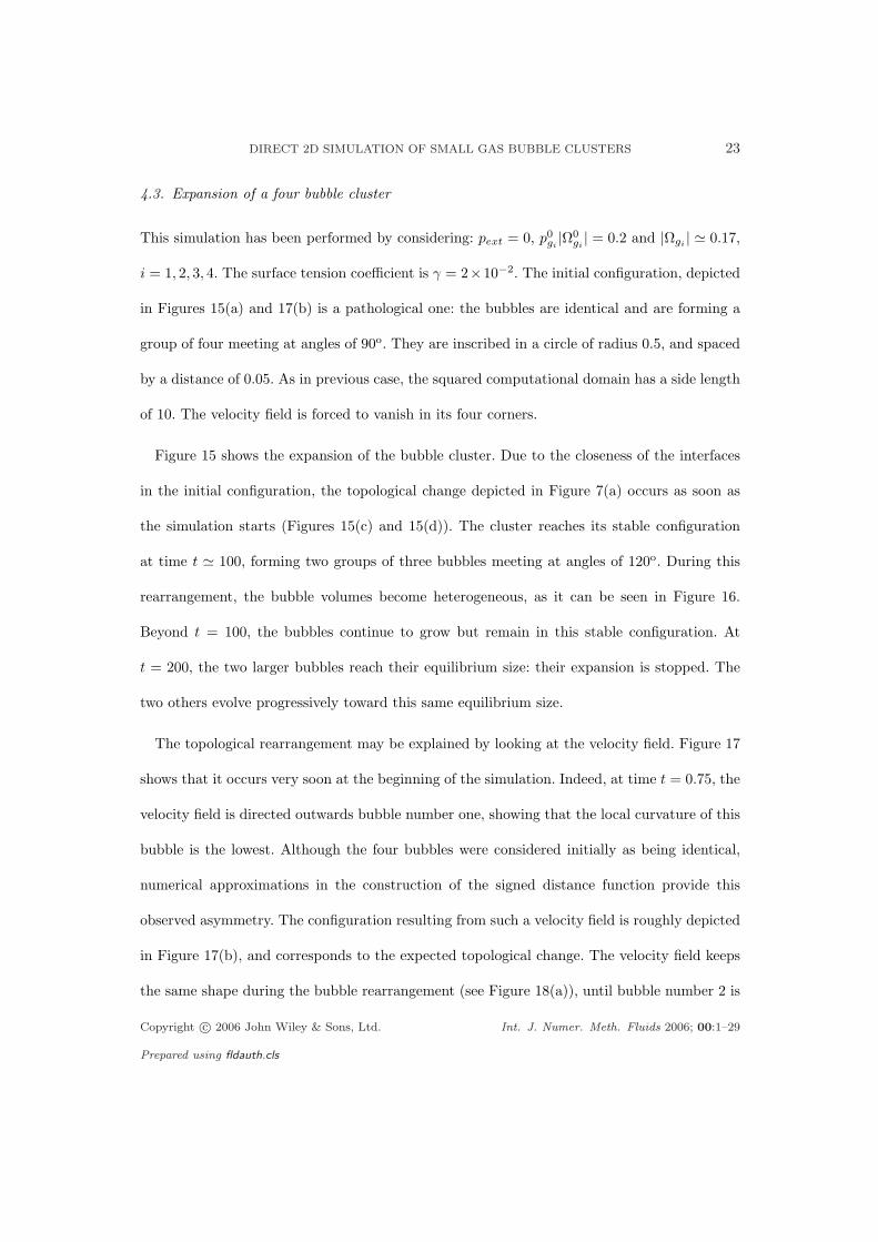
The topological rearrangement may be explained by looking at the velocity field. Figure 17

shows that it occurs very soon at the beginning of the simulation. Indeed, at time t = 0.75, the

velocity field is directed outwards bubble number one, showing that the local curvature of this

bubble is the lowest. Although the four bubbles were considered initially as being identical,

numerical approximations in the construction of the signed distance function provide this

observed asymmetry. The configuration resulting from such a velocity field is roughly depicted

in Figure 17(b), and corresponds to the expected topological change. The velocity field keeps

the same shape during the bubble rearrangement (see Figure 18(a)), until bubble number 2 is




far enough from bubble number 3. Then, the velocity field between bubbles number 1, 2 and 3

from one side, and between bubbles 2, 3 and 4 from the other side, is the same as in the three

bubble case of paragraph 4.2, as shown in Figure 18(b).

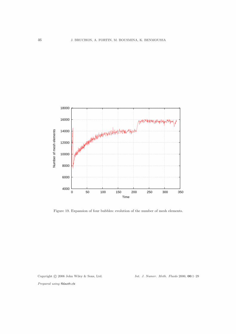
The number of elements provided by the mesh adaptation is plotted in Figure 19. It follows

the evolution of the length of interfaces. The first time steps of the simulation are more difficult

from an adaptation standpoint since the mesh has to reach a prescribed accuracy. This explains

the first jump in the number of elements. The second jump, at t ' 200, corresponds to a change

in the adaptation parameters.

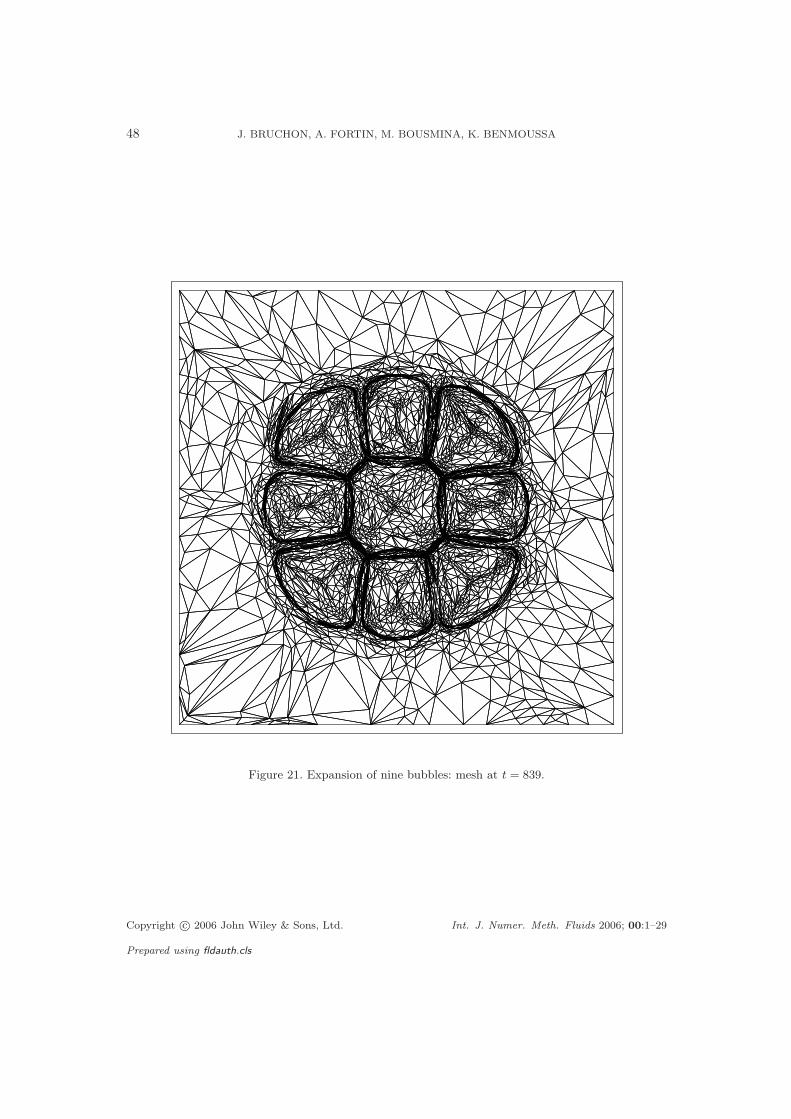
4.4. Expansion of a nine bubble cluster

Finally, the configuration shown in Figure 20(a) is considered: nine spherical bubbles of radius

0.09 are disposed along a regular grid with a center-to-center distance of 0.24. The other

parameters are: pext = 0, p0gi|Ω0

gi| = 2π.10−2 and γ = 10−3. Furthermore, as in previous cases,

the squared computational domain has a side length of 10. The velocity field is enforced to

vanish in its four corners.

The evolution of the cluster, obtained by simulation, is shown in Figure 20 at six different

steps of its expansion. The final mesh is presented in Figure 21 showing how the mesh and

the solution are closely related. Topological changes occur and the Plateau’s rule is clearly

respected: bubbles meet in groups of three, at angles of 120. These topological changes are

similar to the one depicted in Figure 15, except that bubbles have a smaller number of degrees

of freedom for moving. For example, the central bubble can not have any motion of rotation.

Hence, to respect the angles of 120, bubble surfaces must be curved as in Figure 20. Since the

bubbles of Figure 20(f) are not spherical, the equilibrium state is not yet reached. However,




comparison between Figures 20(e) and 20(f) shows that bubbles are slowly recovering their

spherical shape, leading to an increase of the distance separating their surfaces. The simulation

has not been carried out until the equilibrium state is reached, because the process is very slow

and its description requires too thin a mesh for the used numerical method (direct method

to solve the linear system). Regarding the evolution of the cluster, the expected equilibrium

configuration should be similar to the initial one (Figure 20(a)).

5. CONCLUSIONS

A numerical methodology, based on a finite element approach, has been developed for the direct

simulation of small bubble clusters. A velocity-pressure mixed formulation has been established

over the whole computational domain, by extending to the gaseous part, the velocity and the

pressure fields, already defined in the liquid part by Stokes’ equations. The liquid-gas coupling

has been performed through the gas pressure and the surface tension. The gas pressure is

uniform inside each bubble and is related to its volume through an ideal gas law. A level set

method, combined with a mesh adaptation technique, has been used to track the interfaces.

Since one single distance function has been considered to describe all the bubbles, a special

algorithm has been developed to calculate the individual volume of each bubble, which is

required for the gas pressure computation.

The expansion of one single bubble has been investigated. Comparisons with an analytical

model and with the Laplace’s law predictions, have proved the accuracy of the presented

approach, especially for the liquid-gas coupling. These comparisons have revealed the

importance of the boundary effects, occurring if the computational domain characteristic

length is not large enough.




The expansion of small bubble clusters (3, 4 and 9 bubbles) has been successfully simulated.

Topological rearrangements occur during the simulations, giving rise to a transient step, in

which different bubble sizes may appear. Finally, an equilibrium state is nearly reached, in

which only three-bubble groups meeting at angles of 120o are present, as predicted by Plateau’s

rule.

The presented approach allows to combine both the gas compressibility (involved in an

expansion step, for instance) and the minimization of the interfaces, through the action of

surface tension. It makes possible the investigation of the bubble cluster evolution far from the

equilibrium state, as well as near an equilibrium state, through the description of the bubble

shapes, of the velocity field inside the liquid and of the gas pressure.

This work can be improved in many ways. Firstly, by reducing the CPU time of the

computations. Actually, the presented simulations takes several days, running on a processor

Xeon 2,4 GHz, with meshes of about 7000 nodes. This high CPU time cost limits the bubble

number to around ten. On a physical viewpoint, gas diffusion could be investigated in order

to have a more realistic expansion step. Taking into account the disjoining pressure could also

improve the physics of the simulation, allowing to obtain equilibrium states in which bubbles

are not spherical any more.

REFERENCES

1. F.J. Almgren and J.E. Taylor. The Geometry of Soap Films and Soap Bubbles. Scientific American,

235:82–93, 1976.

2. Y. Belhamadia, A. Fortin, and A. Chamberland. Three-dimensional Anisotropic Mesh Adaptation for

Phase Change Problems. J. of Comp. Phys., 201(2):753–770, 2004.




3. Y. Belhamadia, A. Fortin, and E. Chamberland. Mesh Adaptation for the Solution of the Stefan Problem.

J. of Comp. Phys., 194(1):233–255, 2004.

4. A. Beliveau, A. Fortin, and Y. Demay. A Two-dimensional Numerical Method for the Deformation of

Drops with Surface Tension. Int. J. Comp. Fluid Dyn., 10:225–240, 1998.

5. J. U. Brackbill, D. B. Kothe, and C. Zemach. A Continum Method for Modeling Surface Tension. J.

Comp. Phys., 100:335–383, 1992.

6. K. Brakke. The Surface Evolver. Experimental Mathematics, 1(2):141–165, 1992.

7. A. N. Brooks and T.J.R. Hughes. Streamline upwind/Petrov-Galerkin formulations for convection

dominated flows with particular emphasis on the incompressible Navier-Stokes equations. Computer

Methods in Applied Mechanics and Engineering, 32:199–259, 1982.

8. J. Bruchon. Etude de la formation d’une structure de mousse par simulation directe de l’expansion de

bulles dans une matrice liquide polymere. PhD thesis, Ecole Nationale Superieure des Mines de Paris,

2004.

9. A. Caboussat, M. Picasso, and J. Rappaz. Numerical simulation of free surface incompressible liquid flows

surrounded by compressible gas. J. of Comp. Phys., 203(2):626–649, 2005.

10. S.J. Cox, M.F. Vaz, and D Weaire. Topological changes in a two-dimensional foam cluster. Eur. Phys.

J. E, 11:29–35, 2003.

11. S.J. Cox, D. Weaire, and M.F. Vaz. The transition from two-dimensional to three-dimensional foam

structures. Eur. Phys. J. E, 7:311–315, 2002.

12. S.L. Everitt, O.G. Harlen, H.J. Wilson, and D.J. Read. Bubble dynamics in viscoelastic fluids with

application to reacting and non-reacting polymer foams. J. Non-Newtonian Fluid Mech., 114:83–107,

2003.

13. A. Fortin and K. Benmoussa. An adaptative remeshing strategy for free-surface fluid flow problems. Part

I: the axisymmetric case. Journal of Poylmer Eng., 2006. In press.

14. A. Fortin and K. Benmoussa. Numerical simulation of the interaction between fluid drops in multi-phase

flows. J. Comp. Physics, 2006. Submitted.

15. F. Graner. Morphology of Condensed Matter - Physics and Geometry of Spatially Complex Systems.

Springer, 2002.

16. A. Martin S. Hutzler N. Kern, D. Weaire and S. J. Cox. Two-dimensional viscous froth model for foam

dynamics. Physical Review E, 70, 2004.

17. J.A. Sethian. Level Sets Methods and Fast Marching Methods, volume 3. Cambridge Monograph on




applied and computational mathematics, 1986.

18. M. Sussman and E. Fatemi. An Efficient Interface Preserving Level Set Re-Distancing Algorithm and its

Application to Interfacial Incompressible Fluid Flow. SIAM J. Sci. Comp., 20(4):1165–1191, 1999.

19. M. F. Vaz, S.J. Cox, and M.D. Alonso. Minimum energy configurations of small bidisperse bubble clusters.

J. Phys.: Condens. Matter, 16:4165–4175, 2004.

20. D. Weaire, S.J. Cox, and F. Graner. Uniqueness, stability and Hessian eigenvalues for two-dimensional

bubble clusters. Eur. Phys. J. E, 7:123–127, 2002.

21. D. Weaire and S. Hutzler. The Physics of Foams. Oxford, 1999.




Ωg, pg

n

Ωm

σn = −pextn

n

σn

=−

pe

xt n

1/κ

σn = −pextn

n

n

σn = −pextn

n

Figure 1. Expansion of a gas bubble into a liquid matrix.




R

Ωg

x

Symmetry axis: uy = 0

y

free boundary: σn = 0

Characteristic length

σn = 0

liquid matrix Ωm

ux = 0

Figure 2. Computational domain for the expansion of a single gas bubble




Figure 3. Expansion of a gas bubble: interface and first component of the velocity field.




0.1

0.2

0.3

0.4

0.5

0.6

0.7

0.8

0.9

0 50 100 150 200 250

Rad

ius

Time

Without mesh adaptationWith mesh adaptationAnalytical expression

(a) Bubble radius: comparison between theory and simulation

0

0.02

0.04

0.06

0.08

0.1

0.12

0.14

0.16

0.18

0.2

0.22

0 50 100 150 200 250

Rel

ativ

e er

ror

Time

Without adaptationWith adaptation

(b) Relative error |R−Rh|/R

Figure 4. Expansion of a disk of initial radius 0.1 into a domain of length 1.




0

0.5

1

1.5

2

2.5

3

0 500 1000 1500 2000 2500 3000 3500 4000

Rad

ius

Time

SimulationAnalytical model

(a) Bubble radius: comparison between theory and simulation

0.006

0.008

0.01

0.012

0.014

0.016

0.018

0.02

0.022

0.024

0.026

0 500 1000 1500 2000 2500 3000 3500 4000

Rel

ativ

e er

ror

Time

(b) Relative error |R−Rh|/R

Figure 5. Expansion of a disk of initial radius 0.1 into a domain of length 10.




0.11

0.12

0.13

0.14

0.15

0.16

0.17

0.18

0.19

0.2

0.21

0 50 100 150 200 250 300 350 400 450 500

Rad

ius

Time

With surface tension

(a) Bubble radius evolution

0.04

0.05

0.06

0.07

0.08

0.09

0.1

0.11

0.12

0.13

0.14

0 50 100 150 200 250 300 350 400 450 500

Bub

ble

pres

sure

Time

With surface tension

(b) Bubble pressure evolution

Figure 6. Expansion of a disk of initial radius 0.1 and initial pressure 0.2, into a domain of length 10,

with surface tension effect.




Bubble 1

Bubble 1

Bubble 3

Bubble 3

Bubble 2

Bubble 2Bubble 4

Bubble 1

Bubble 4

Bubble 4

Bubble 3

Bubble 2

(a) Topological changes in a four bubble cluster.

Bubble 2Bubble 3

Bubble 1

120 degrees

(b) Three bubbles at 120 degree

angles.

Figure 7. Plateau’s rule.




(a) t = 0 (b) t = 1.4

(c) t = 10 (d) t = 37

(e) t = 284 (f) t = 824

Figure 8. Expansion of three bubbles.




(a) t = 0 (b) t = 1.4

(c) t = 10 (d) t = 37

(e) t = 284 (f) t = 824

Figure 9. Expansion of three bubbles: meshes.




(a) t = 1.4

(b) t = 10

Figure 10. Expansion of three bubbles: velocity field (first stage of the expansion.)Copyright c© 2006 John Wiley & Sons, Ltd. Int. J. Numer. Meth. Fluids 2006; 00:1–29



Bubble 3

Bubble 1

Bubble 2

R3

C3

R1

C2R2

C1α1

α3α2

(a) Unstable state

Bubble 3

Bubble 1

Bubble 2

(b) Velocity due to the difference of curvatures

Figure 11. Plateau’s rule: three bubbles going to their equilibrium state.Copyright c© 2006 John Wiley & Sons, Ltd. Int. J. Numer. Meth. Fluids 2006; 00:1–29



(a) t = 73

(b) t = 670

Figure 12. Expansion of three bubbles: velocity field (last two stages of the expansion.)Copyright c© 2006 John Wiley & Sons, Ltd. Int. J. Numer. Meth. Fluids 2006; 00:1–29



0

0.5

1

1.5

2

2.5

3

0 100 200 300 400 500 600 700 800 900

Vol

ume

Time

Bubble 1Bubble 2Bubble 3

Figure 13. Expansion of three bubbles: evolution of their volumes.

2000

4000

6000

8000

10000

12000

14000

16000

18000

0 100 200 300 400 500 600 700 800 900

Num

ber

of m

esh

elem

ents

Time

Figure 14. Expansion of three bubbles: evolution of the number of mesh elements.




(a) t = 0 (b) t = 7

(c) t = 23 (d) t = 59

(e) t = 225 (f) t = 322

Figure 15. Expansion of four bubbles.




0

0.5

1

1.5

2

2.5

3

3.5

4

4.5

5

0 50 100 150 200 250 300 350

Vol

ume

of b

ubbl

es

Time

Bubble 1Bubble 2Bubble 3Bubble 4

Figure 16. Expansion of four bubbles: evolution of their volumes.




(a) t = 0.75

Bubble 1 Bubble 2

Bubble 4Bubble 3

Bubble 1 Bubble 2

Bubble 4Bubble 3

(b) Topological rearrangement: rough description of the velocity field at t = 0.75 and

induced configuration

Figure 17. Expansion of four bubbles: velocity field (first stage of the expansion.)




(a) t = 7

(b) t = 37

Figure 18. Expansion of four bubbles: velocity field (first and middle stages of the expansion.)Copyright c© 2006 John Wiley & Sons, Ltd. Int. J. Numer. Meth. Fluids 2006; 00:1–29



4000

6000

8000

10000

12000

14000

16000

18000

0 50 100 150 200 250 300 350

Num

ber

of m

esh

elem

ents

Time

Figure 19. Expansion of four bubbles: evolution of the number of mesh elements.




(a) t = 0 (b) t = 47

(c) t = 263 (d) t = 534

(e) t = 800 (f) t = 839

Figure 20. Expansion of nine bubbles.




Figure 21. Expansion of nine bubbles: mesh at t = 839.



Documents

Direct 2D simulation of small gas bubble clusters: from ...bruchon/articles/bruchon_fortin.pdf · 1 GIREF, D¶epartement de math¶ematiques et de statistique, Universit¶e Laval,