Embed Size (px)
Citation preview
DimmWitted: A Study of Main-Memory Statistical Analytics
Ce Zhang†‡ Christopher Re††Stanford University
‡University of Wisconsin-Madison
{czhang, chrismre}@cs.stanford.edu
ABSTRACTWe perform the first study of the tradeoff space of accessmethods and replication to support statistical analytics us-ing first-order methods executed in the main memory of aNon-Uniform Memory Access (NUMA) machine. Statisticalanalytics systems differ from conventional SQL-analytics inthe amount and types of memory incoherence that they cantolerate. Our goal is to understand tradeoffs in accessing thedata in row- or column-order and at what granularity oneshould share the model and data for a statistical task. Westudy this new tradeoff space and discover that there aretradeoffs between hardware and statistical efficiency. Weargue that our tradeoff study may provide valuable infor-mation for designers of analytics engines: for each systemwe consider, our prototype engine can run at least one pop-ular task at least 100× faster. We conduct our study acrossfive architectures using popular models, including SVMs, lo-gistic regression, Gibbs sampling, and neural networks.
1. INTRODUCTIONStatistical data analytics is one of the hottest topics in
data-management research and practice. Today, even smallorganizations have access to machines with large main mem-ories (via Amazon’s EC2) or for purchase at $5/GB. As aresult, there has been a flurry of activity to support main-memory analytics in both industry (Google Brain, Impala,and Pivotal) and research (GraphLab, and MLlib). Eachof these systems picks one design point in a larger tradeoffspace. The goal of this paper is to define and explore thisspace. We find that today’s research and industrial systemsunder-utilize modern commodity hardware for analytics—sometimes by two orders of magnitude. We hope that ourstudy identifies some useful design points for the next gen-eration of such main-memory analytics systems.
Throughout, we use the term statistical analytics to referto those tasks that can be solved by first-order methods–aclass of iterative algorithms that use gradient information;
these methods are the core algorithm in systems such as ML-lib, GraphLab, and Google Brain. Our study examines an-alytics on commodity multi-socket, multi-core, non-uniformmemory access (NUMA) machines, which are the de factostandard machine configuration and thus a natural target foran in-depth study. Moreover, our experience with severalenterprise companies suggests that, after appropriate pre-processing, a large class of enterprise analytics problems fitinto the main memory of a single, modern machine. Whilethis architecture has been recently studied for traditionalSQL-analytics systems [16], it has not been studied for sta-tistical analytics systems.
Statistical analytics systems are different from traditionalSQL-analytics systems. In comparison to traditional SQL-analytics, the underlying methods are intrinsically robust toerror. On the other hand, traditional statistical theory doesnot consider which operations can be efficiently executed.This leads to a fundamental tradeoff between statistical ef-ficiency (how many steps are needed until convergence toa given tolerance) and hardware efficiency (how efficientlythose steps can be carried out).
To describe such tradeoffs more precisely, we describe thesetup of the analytics tasks that we consider in this paper.The input data is a matrix in RN×d and the goal is to finda vector x ∈ Rd that minimizes some (convex) loss function,say the logistic loss or the hinge loss (SVM). Typically, onemakes several complete passes over the data while updatingthe model; we call each such pass an epoch. There may besome communication at the end of the epoch, e.g., in bulk-synchronous parallel systems such as Spark. We identifythree tradeoffs that have not been explored in the literature:(1) access methods for the data, (2) model replication, and(3) data replication. Current systems have picked one pointin this space; we explain each space and discover pointsthat have not been previously considered. Using these newpoints, we can perform 100× faster than previously exploredpoints in the tradeoff space for several popular tasks.
Access Methods. Analytics systems access (and store) datain either row-major or column-major order. For example,systems that use stochastic gradient descent methods (SGD)access the data row-wise; examples include MADlib [23]in Impala and Pivotal, Google Brain [29], and MLlib inSpark [47]; and stochastic coordinate descent methods (SCD)access the data column-wise; examples include GraphLab [34],Shogun [46], and Thetis [48]. These methods have essen-tially identical statistical efficiency, but their wall-clock per-formance can be radically different due to hardware effi-
1
arX
iv:1
403.
7550
v3 [
cs.D
B]
7 J
ul 2
014

Node 2
L3 Cache RAM
Core3 Core4
N
d
(a) Memory Model for DimmWitted
Data A Model x Machine Node 1
L3 Cache RAM
Core1 Core2
d
Goal
(d) NUMA Architecture (c) Access Methods
Row-wise Col.-wise Col.-to-row
Read set of data Write set of model
(b) Pseudocode of SGD
Procedure: m <-- initial model while not converge foreach row z in A: m <-- m – α grad(z, m) test convergence
Input: Data matrix A, stepsize α Gradient function grad. Output: Model m.
Epoch
L1/L2 L1/L2 L1/L2 L1/L2
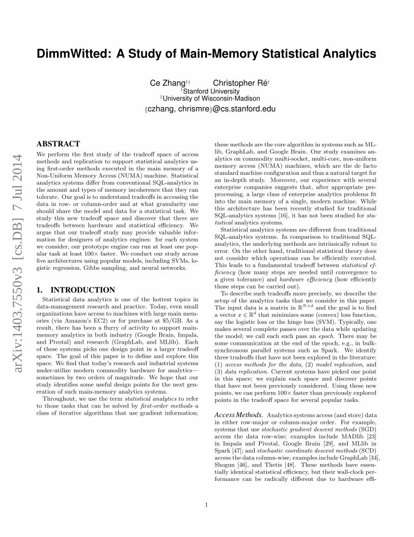
Figure 1: Illustration of (a) DimmWitted’s Memory Model, (b) Pseudocode for SGD, (c) Different StatisticalMethods in DimmWitted and Their Access Patterns, and (d) NUMA Architecture.
ciency. However, this tradeoff has not been systematicallystudied. To study this tradeoff, we introduce a storage ab-straction that captures the access patterns of popular statis-tical analytics tasks and a prototype called DimmWitted.In particular, we identify three access methods that are usedin popular analytics tasks, including standard supervisedmachine learning models such as SVMs, logistic regression,and least squares; and more advanced methods such as neu-ral networks and Gibbs sampling on factor graphs. For dif-ferent access methods for the same problem, we find that thetime to converge to a given loss can differ by up to 100×.
We also find that no access method dominates all oth-ers, so an engine designer may want to include both accessmethods. To show that it may be possible to support bothmethods in a single engine, we develop a simple cost modelto choose among these access methods. We describe a sim-ple cost model that selects a nearly optimal point in ourdata sets, models, and different machine configurations.
Data and Model Replication. We study two sets of trade-offs: the level of granularity, and the mechanism by whichmutable state and immutable data are shared in analyticstasks. We describe the tradeoffs we explore in both (1) mu-table state sharing, which we informally call model replica-tion, and (2) data replication.
(1) Model Replication. During execution, there is somestate that the task mutates (typically an update to themodel). We call this state, which may be shared amongone or more processors, a model replica. We consider threedifferent granularities at which to share model replicas:
• The PerCore approach treats a NUMA machine as adistributed system in which every core is treated as anindividual machine, e.g., in bulk-synchronous modelssuch as MLlib on Spark or event-driven systems such asGraphLab. These approaches are the classical shared-nothing and event-driven architectures, respectively.In PerCore, the part of the model that is updated byeach core is only visible to that core until the end ofan epoch. This method is efficient and scalable froma hardware perspective, but it is less statistically ef-ficient, as there is only coarse-grained communicationbetween cores.
• The PerMachine approach acts as if each processor hasuniform access to memory. This approach is taken inHogwild! and Google Downpour [19]. In this method,the hardware takes care of the coherence of the shared
state. The PerMachine method is statistically efficientdue to high communication rates, but it may causecontention in the hardware, which may lead to subop-timal running times.
• A natural hybrid is PerNode; this method uses thefact that PerCore communication through the last-levelcache (LLC) is dramatically faster than communica-tion through remote main memory. This method isnovel; for some models, PerNode can be an order ofmagnitude faster.
Because model replicas are mutable, a key question is howoften should we synchronize model replicas? We find that itis beneficial to synchronize the models as much as possible—so long as we do not impede throughput to data in mainmemory. A natural idea, then, is to use PerMachine sharing,in which the hardware is responsible for synchronizing thereplicas. However, this decision can be suboptimal, as thecache-coherence protocol may stall a processor to preservecoherence, but this information may not be worth the costof a stall from a statistical efficiency perspective. We findthat the PerNode method, coupled with a simple techniqueto batch writes across sockets, can dramatically reduce com-munication and processor stalls. The PerNode method canresult in an over 10× runtime improvement. This techniquedepends on the fact that we do not need to maintain themodel consistently: we are effectively delaying some updatesto reduce the total number of updates across sockets (whichlead to processor stalls).
(2) Data Replication. The data for analytics is immutable,so there are no synchronization issues for data replication.The classical approach is to partition the data to take ad-vantage of higher aggregate memory bandwidth. However,each partition may contain skewed data, which may slowconvergence. Thus, an alternate approach is to replicate thedata fully (say, per NUMA node). In this approach, eachnode accesses that node’s data in a different order, whichmeans that the replicas provide non-redundant statisticalinformation; in turn, this reduces the variance of the esti-mates based on the data in each replicate. We find that forsome tasks, fully replicating the data four ways can convergeto the same loss almost 4× faster than the sharding strategy.
Summary of Contributions. We are the first to study thethree tradeoffs listed above for main-memory statistical an-alytics systems. These tradeoffs are not intended to be anexhaustive set of optimizations, but they demonstrate our
2

main conceptual point: treating NUMA machines as dis-tributed systems or SMP is suboptimal for statistical ana-lytics. We design a storage manager, DimmWitted, thatshows it is possible to exploit these ideas on real data sets.Finally, we evaluate our techniques on multiple real datasets,models, and architectures.
2. BACKGROUNDIn this section, we describe the memory model for
DimmWitted, which provides a unified memory model toimplement popular analytics methods. Then, we recall somebasic properties of modern NUMA architectures.
Data for Analytics. The data for an analytics task is apair (A, x), which we call the data and the model, respec-tively. For concreteness, we consider a matrix A ∈ RN×d.In machine learning parlance, each row is called an exam-ple. Thus, N is often the number of examples and d is oftencalled the dimension of the model. There is also a model,typically a vector x ∈ Rd. The distinction is that the dataA is read-only, while the model vector, x, will be updatedduring execution. From the perspective of this paper, theimportant distinction we make is that data is an immutablematrix, while the model (or portions of it) are mutable data.
First-Order Methods for Analytic Algorithms. DimmWit-ted considers a class of popular algorithms called first-ordermethods. Such algorithms make several passes over the data;we refer to each such pass as an epoch. A popular exam-ple algorithm is stochastic gradient descent (SGD), whichis widely used by web-companies, e.g., Google Brain [29]and VowPal Wabbit [1], and in enterprise systems such asPivotal, Oracle, and Impala. Pseudocode for this methodis shown in Figure 1(b). During each epoch, SGD reads asingle example z; it uses the current value of the model andz to estimate the derivative; and it then updates the modelvector with this estimate. It reads each example in this loop.After each epoch, these methods test convergence (usuallyby computing or estimating the norm of the gradient); thiscomputation requires a scan over the complete dataset.
2.1 Memory Models for AnalyticsWe design DimmWitted’s memory model to capture the
trend in recent high-performance sampling and statisticalmethods. There are two aspects to this memory model: thecoherence level and the storage layout.
Coherence Level. Classically, memory systems are coher-ent: reads and writes are executed atomically. For analyticssystems, we say that a memory model is coherent if readsand writes of the entire model vector are atomic. That is,access to the model is enforced by a critical section. How-ever, many modern analytics algorithms are designed for anincoherent memory model. The Hogwild! method showedthat one can run such a method in parallel without lockingbut still provably converge. The Hogwild! memory modelrelies on the fact that writes of individual components areatomic, but it does not require that the entire vector beupdated atomically. However, atomicity at the level of thecacheline is provided by essentially all modern processors.Empirically, these results allow one to forgo costly locking(and coherence) protocols. Similar algorithms have been
Algorithm Access Method Implementation
Stochastic Gradient Descent Row-wise MADlib, Spark, Hogwild!
Stochastic Coordinate Descent Column-wise
GraphLab, Shogun, Thetis Column-to-row
Figure 2: Algorithms and Their Access Methods.
proposed for other popular methods, including Gibbs sam-pling [25, 45], stochastic coordinate descent (SCD) [42, 46],and linear systems solvers [48]. This technique was appliedby Dean et al. [19] to solve convex optimization problemswith billions of elements in a model. This memory model isdistinct from the classical, fully coherent database execution.
The DimmWitted prototype allows us to specify that aregion of memory is coherent or not. This region of memorymay be shared by one or more processors. If the memoryis only shared per thread, then we can simulate a shared-nothing execution. If the memory is shared per machine, wecan simulate Hogwild!.
Access Methods. We identify three distinct access pathsused by modern analytics systems, which we call row-wise,column-wise, and column-to-row. They are graphically il-lustrated in Figure 1(c). Our prototype supports all threeaccess methods. All of our methods perform several epochs,that is, passes over the data. However, the algorithm mayiterate over the data row-wise or column-wise.
• In row-wise access, the system scans each row of thetable and applies a function that takes that row, ap-plies a function to it, and then updates the model.This method may write to all components of themodel. Popular methods that use this access methodinclude stochastic gradient descent, gradient descent,and higher-order methods (such as l-BFGS).
• In column-wise access, the system scans each column jof the table. This method reads just the j componentof the model. The write set of the method is typicallya single component of the model. This method is usedby stochastic coordinate descent.
• In column-to-row access, the system iterates conceptu-ally over the columns. This method is typically appliedto sparse matrices. When iterating on column j, itwill read all rows in which column j is non-zero. Thismethod also updates a single component of the model.This method is used by non-linear support vector ma-chines in GraphLab and is the de facto approach forGibbs sampling.
DimmWitted is free to iterate over rows or columns in es-sentially any order (although typically some randomness inthe ordering is desired). Figure 2 classifies popular imple-mentations by their access method.
2.2 Architecture of NUMA MachinesWe briefly describe the architecture of a modern NUMA
machine. As illustrated in Figure 1(d), a NUMA machinecontains multiple NUMA nodes. Each node has multiplecores and processor caches, including the L3 cache. Each
3

Wor
ker
RA
M 6GB/s
QPI 11GB/s
Name (abbrv.) #Node #Cores/
Node RAM/
Node (GB) CPU
Clock (GHz) LLC (MB)
local2 (l2) 2 6 32 2.6 12
local4 (l4) 4 10 64 2.0 24
local8 (l8) 8 8 128 2.6 24
ec2.1 (e1) 2 8 122 2.6 20
ec2.2 (e2) 2 8 30 2.6 20
local2
Wor
ker
RA
M 6GB/s
Figure 3: Summary of Machines and Memory Band-width on local2 Tested with STREAM [9].
Data A
Machine
…
…
Data Replica
Model Replica
Worker
Read Update Execution Plan
Model x
Optim
izer
Figure 4: Illustration of DimmWitted’s Engine.
node is directly connected to a region of DRAM. NUMAnodes are connected to each other by buses on the mainboard; in our case, this connection is the Intel Quick PathInterconnects (QPIs), which has a bandwidth as high as25.6GB/s.1 To access DRAM regions of other NUMA nodes,data is transferred across NUMA nodes using the QPI. TheseNUMA architectures are cache coherent, and the coherencyactions use the QPI. Figure 3 describes the configurationof each machine that we use in this paper. Machines con-trolled by us have names with the prefix “local”; the othermachines are Amazon EC2 configurations.
3. THE DIMMWITTED ENGINEWe describe the tradeoff space that DimmWitted’s op-
timizer considers, namely (1) access method selection, (2)model replication, and (3) data replication. To help un-derstand the statistical-versus-hardware tradeoff space, wepresent some experimental results in a Tradeoffs paragraphwithin each subsection. We describe implementation detailsfor DimmWitted in the full version of this paper.
3.1 System OverviewWe describe analytics tasks in DimmWitted and the ex-
ecution model of DimmWitted given an analytics task.
System Input. For each analytics task that we study, weassume that the user provides data A ∈ RN×d and an initialmodel that is a vector of length d. In addition, for eachaccess method listed above, there is a function of an ap-propriate type that solves the same underlying model. Forexample, we provide both a row- and column-wise way ofsolving a support vector machine. Each method takes twoarguments; the first is a pointer to a model.
1www.intel.com/content/www/us/en/io/quickpath-technology/quick-path-interconnect-introduction-paper.html
Tradeoff Strategies Existing Systems
Access Methods
Row-wise SP, HW Column-wise GL Column-to-row
Model Replication
Per Core GL, SP Per Node
Per Machine HW Data
Replication Sharding GL, SP, HW
Full Replication
Figure 5: A Summary of DimmWitted’s Tradeoffsand Existing Systems (GraphLab (GL), Hogwild!(HW), Spark (SP)).
• frow captures the the row-wise access method, and itssecond argument is the index of a single row.
• fcol captures the column-wise access method, and itssecond argument is the index of a single column.
• fctr captures the column-to-row access method, andits second argument is a pair of one column index anda set of row indexes. These rows correspond to thenon-zero entries in a data matrix for a single column.2
Each of the functions modifies the model to which they re-ceive a pointer in place. However, in our study, frow canmodify the whole model, while fcol and fctr only modify asingle variable of the model. We call the above tuple of func-tions a model specification. Note that a model specificationcontains either fcol or fctr but typically not both.
Execution. Given a model specification, our goal is to gen-erate an execution plan. An execution plan, schematicallyillustrated in Figure 4, specifies three things for each CPUcore in the machine: (1) a subset of the data matrix to op-erate on, (2) a replica of the model to update, and (3) theaccess method used to update the model. We call the set ofreplicas of data and models locality groups, as the replicasare described physically; i.e., they correspond to regions ofmemory that are local to particular NUMA nodes, and oneor more workers may be mapped to each locality group. Thedata assigned to distinct locality groups may overlap. Weuse DimmWitted’s engine to explore three tradeoffs:
(1) Access methods, in which we can select betweeneither the row or column method to access the data.
(2) Model replication, in which we choose how to createand assign replicas of the model to each worker. Whena worker needs to read or write the model, it will reador write the model replica that it is assigned.
(3) Data replication, in which we choose a subset of datatuples for each worker. The replicas may be overlap-ping, disjoint, or some combination.
Figure 5 summarizes the tradeoff space. In each section,we illustrate the tradeoff along two axes, namely (1) thestatistical efficiency, i.e., the number of epochs it takes toconverge, and (2) hardware efficiency, the time that eachmethod takes to finish a single epoch.
2Define S(j) = {i : aij 6= 0}. For a column j, the input tofctr is a pair (j, S(j)).
4

Algorithm Read Write (Dense) Write (Sparse) Row-wise
Column-wise
Column-to-row
ni∑d
dN
ni2∑ni∑
ni∑
Figure 6: Per Epoch Execution Cost of Row- andColumn-wise Access. The Write column is for a single
model replica. Given a dataset A ∈ RN×d, let ni be the
number of non-zero elements ai.
0.01
0.1
1
10
0.1 1 10 Tim
e/Ep
och
(sec
onds
)
Cost Ratio
Row-wise
Column-wise
(a) Number of Epochs to Converge (b) Time for Each Epoch
1
10
100
SVM1 SVM2 LP1 LP2
# Ep
och
Models and Data Sets
Column-wise Row-wise
Figure 7: Illustration of the Method SelectionTradeoff. (a) These four datasets are RCV1, Reuters,
Amazon, and Google, respectively. (b) The “cost ratio”
is defined as the ratio of costs estimated for row-wise and
column-wise methods: (1+α)∑
i ni/(∑
i n2i +αd), where ni
is the number of non-zero elements of ith row of A and
α is the cost ratio between writing and reads. We set
α = 10 to plot this graph.
3.2 Access Method SelectionIn this section, we examine each access method: row-wise,
column-wise, and column-to-row. We find that the execu-tion time of an access method depends more on hardwareefficiency than on statistical efficiency.
Tradeoffs. We consider the two tradeoffs that we use fora simple cost model (Figure 6). Let ni be the number ofnon-zeros in row i; when we store the data as sparse vec-tors/matrices in CSR format, the number of reads in a row-
wise access method is∑N
i=1 ni. Since each example is likelyto be written back in a dense write, we perform dN writesper epoch. Our cost model combines these two costs lin-early with a factor α that accounts for writes being moreexpensive, on average, because of contention. The factor αis estimated at installation time by measuring on a small setof datasets. The parameter α is in 4 to 12 and grows withthe number of sockets; e.g., for local2, α ≈ 4, and for local8,α ≈ 12. Thus, α may increase in the future.
Statistical Efficiency. We observe that each accessmethod has comparable statistical efficiency. To illustratethis, we run all methods on all of our datasets and reportthe number of epochs that one method converges to a givenerror to the optimal loss, and Figure 7(a) shows the resulton four datasets with 10% error. We see that the gap in thenumber of epochs across different methods is small (alwayswithin 50% of each other).
Hardware Efficiency. Different access methods canchange the time per epoch by up to a factor of 10×, andthere is a cross-over point. To see this, we run both meth-ods on a series of synthetic datasets where we control thenumber of non-zero elements per row by subsampling each
row on the Music dataset (see Section 4 for more details).For each subsampled dataset, we plot the cost ratio on thex-axis, and we plot their actual running time per epoch inFigure 7(b). We see a cross-over point on the time usedper epoch: when the cost ratio is small, row-wise outper-forms column-wise by 6×, as the column-wise method readsmore data; on the other hand, when the ratio is large, thecolumn-wise method outperforms the row-wise method by3×, as the column-wise method has lower write contention.We observe similar cross-over points on our other datasets.
Cost-based Optimizer. DimmWitted estimates the exe-cution time of different access methods using the number ofbytes that each method reads and writes in one epoch, asshown in Figure 6. For writes, it is slightly more complex:for models such as SVM, each gradient step in row-wise ac-cess only updates the coordinates where the input vectorcontains non-zero elements. We call this scenario a sparseupdate; otherwise, it is a dense update.
DimmWitted needs to estimate the ratio of the cost ofreads to writes. To do this, it runs a simple benchmarkdataset. We find that, for all the eight datasets, five statis-tical models, and five machines that we use in the experi-ments, the cost model is robust to this parameter: as longas writes are 4× to 100× more expensive than reading, thecost model makes the correct decision between row-wise andcolumn-wise access.
3.3 Model ReplicationIn DimmWitted, we consider three model replication
strategies. The first two strategies, namely PerCore andPerMachine, are similar to traditional shared-nothing andshared-memory architecture, respectively. We also considera hybrid strategy, PerNode, designed for NUMA machines.
3.3.1 Granularity of Model ReplicationThe difference between the three model replication strate-
gies is the granularity of replicating a model. We first de-scribe PerCore and PerMachine and their relationship withother existing systems (Figure 5). We then describe PerN-ode, a simple, novel hybrid strategy that we designed toleverage the structure of NUMA machines.
PerCore. In the PerCore strategy, each core maintains a mu-table state, and these states are combined to form a newversion of the model (typically at the end of each epoch).This is essentially a shared-nothing architecture; it is imple-mented in Impala, Pivotal, and Hadoop-based frameworks.PerCore is popularly implemented by state-of-the-art sta-tistical analytics frameworks such as Bismarck, Spark, andGraphLab. There are subtle variations to this approach: inBismarck’s implementation, each worker processes a parti-tion of the data, and its model is averaged at the end ofeach epoch; Spark implements a minibatch-based approachin which parallel workers calculate the gradient based onexamples, and then gradients are aggregated by a singlethread to update the final model; GraphLab implementsan event-based approach where each different task is dy-namically scheduled to satisfy the given consistency require-ment. In DimmWitted, we implement PerCore in a waythat is similar to Bismarck, where each worker has its ownmodel replica, and each worker is responsible for updating
5

1
10
100
1000
10000
1% 10% 100%
PerCore #
Epoc
h
Error to Optimal Loss
(a) Number of Epochs to Converge
PerNode
PerMachine
(b) Time for Each Epoch
0.1
1
10
Tim
e/Ep
och
(sec
ond)
Model Replication Strategies
PerMachine
PerCore
PerNode
Figure 8: Illustration of Model Replication.
its replica.3 As we will show in the experiment section,DimmWitted’s implementation is 3-100× faster than eitherGraphLab and Spark. Both systems have additional sourcesof overhead that DimmWitted does not, e.g., for fault tol-erance in Spark and a distributed environment in both. Weare not making an argument about the relative merits ofthese features in applications, only that they would obscurethe tradeoffs that we study in this paper.
PerMachine. In the PerMachine strategy, there is a singlemodel replica that all workers update during execution. Per-Machine is implemented in Hogwild! and Google’s Down-pour. Hogwild! implements a lock-free protocol, whichforces the hardware to deal with coherence. Although differ-ent writers may overwrite each other and readers may havedirty reads, Niu et al. [38] prove that Hogwild! converges.
PerNode. The PerNode strategy is a hybrid of PerCore andPerMachine. In PerNode, each NUMA node has a singlemodel replica that is shared among all cores on that node.
Model Synchronization. Deciding how often the replicassynchronize is key to the design. In Hadoop-based andBismarck-based models, they synchronize at the end of eachepoch. This is a shared-nothing approach that works well inuser-defined aggregations. However, we consider finer gran-ularities of sharing. In DimmWitted, we chose to have onethread that periodically reads models on all other cores, av-erages their results, and updates each replica.
One key question for model synchronization is how fre-quently should the model be synchronized? Intuitively, wemight expect that more frequent synchronization will lowerthe throughput; on the other hand, the more frequently wesynchronize, the fewer number of iterations we might needto converge. However, in DimmWitted, we find that theoptimal choice is to communicate as frequently as possi-ble. The intuition is that the QPI has staggering band-width (25GB/s) compared to the small amount of data weare shipping (megabytes). As a result, in DimmWitted, weimplement an asynchronous version of the model averagingprotocol: a separate thread averages models, with the effectof batching many writes together across the cores into onewrite, reducing the number of stalls.
3We implemented MLlib’s minibatch in DimmWitted. Wefind that the Hogwild!-like implementation always dom-inates the minibatch implementation. DimmWitted’scolumn-wise implementation for PerMachine is similar toGraphLab, with the only difference that DimmWitted doesnot schedule the task in an event-driven way.
1
100
10000
1% 10% 100%
Sharding
FullReplication
(a) Number of Epochs to Converge (b) Time for Each Epoch
0.0001
0.001
0.01
local2 local4 local8
Sharding FullReplication
Tim
e/Ep
och
(sec
onds
)
# Ep
och
Error to Optimal Loss Different Machines
Figure 9: Illustration of Data Replication.
Tradeoffs. We observe that PerNode is more hardware ef-ficient, as it takes less time to execute an epoch than Per-Machine; PerMachine might use fewer number of epochs toconverge than PerNode.
Statistical Efficiency. We observe that PerMachine usu-ally takes fewer epochs to converge to the same loss com-pared to PerNode, and PerNode uses fewer number of epochsthan PerCore. To illustrate this observation, Figure 8(a)shows the number of epochs that each strategy requires toconverge to a given loss for SVM (RCV1). We see thatPerMachine always uses the least number of epochs to con-verge to a given loss: intuitively, the single model replicahas more information at each step, which means that thereis less redundant work. We observe similar phenomena whencomparing PerCore and PerNode.
Hardware Efficiency. We observe that PerNode usesmuch less time to execute an epoch than PerMachine. Toillustrate the difference in the time that each model replica-tion strategy uses to finish one epoch, we show in Figure 8(b)the execution time of three strategies on SVM (RCV1). Wesee that PerNode is 23× faster than PerMachine and that Per-Core is 1.5× faster than PerNode. PerNode takes advantageof the locality provided by the NUMA architecture. UsingPMUs, we find that PerMachine incurs 11× more cross-nodeDRAM requests than PerNode.
Rule of Thumb. For SGD-based models, PerNode usuallygives optimal results, while for SCD-based models, PerMa-chine does. Intuitively, this is caused by the fact that SGDhas a denser update pattern than SCD, so, PerMachine suf-fers from hardware efficiency.
3.4 Data ReplicationIn DimmWitted, each worker processes a subset of data
and then updates its model replica. To assign a subset ofdata to each worker, we consider two strategies.
Sharding. Sharding is a popular strategy implemented in sys-tems such as Hogwild!, Spark, and Bismarck, in which thedataset is partitioned, and each worker only works on its par-tition of data. When there is a single model replica, Shardingavoids wasted computation, as each tuple is processed onceper epoch. However, when there are multiple model repli-cas, Sharding might increase the variance of the estimatewe form on each node, lowering the statistical efficiency. InDimmWitted, we implement Sharding by randomly parti-tioning the rows (resp. columns) of a data matrix for therow-wise (resp. column-wise) access method. In column-to-row access, we also replicate other rows that are needed.
FullReplication. A simple alternative to Sharding is FullRepli-cation, in which we replicate the whole dataset many times
6
Model Dataset #Row #Col. NNZ Size (Sparse)
Size (Dense) Sparse
SVM LR LS
RCV1 781K 47K 60M 914MB 275GB ✔ Reuters 8K 18K 93K 1.4MB 1.2GB ✔ Music 515K 91 46M 701MB 0.4GB Forest 581K 54 30M 490MB 0.2GB
LP Amazon 926K 335K 2M 28MB >1TB ✔ Google 2M 2M 3M 25MB >1TB ✔
QP Amazon 1M 1M 7M 104MB >1TB ✔ Google 2M 2M 10M 152MB >1TB ✔
Gibbs Paleo 69M 30M 108M 2GB >1TB ✔ NN MNIST 120M 800K 120M 2GB >1TB ✔
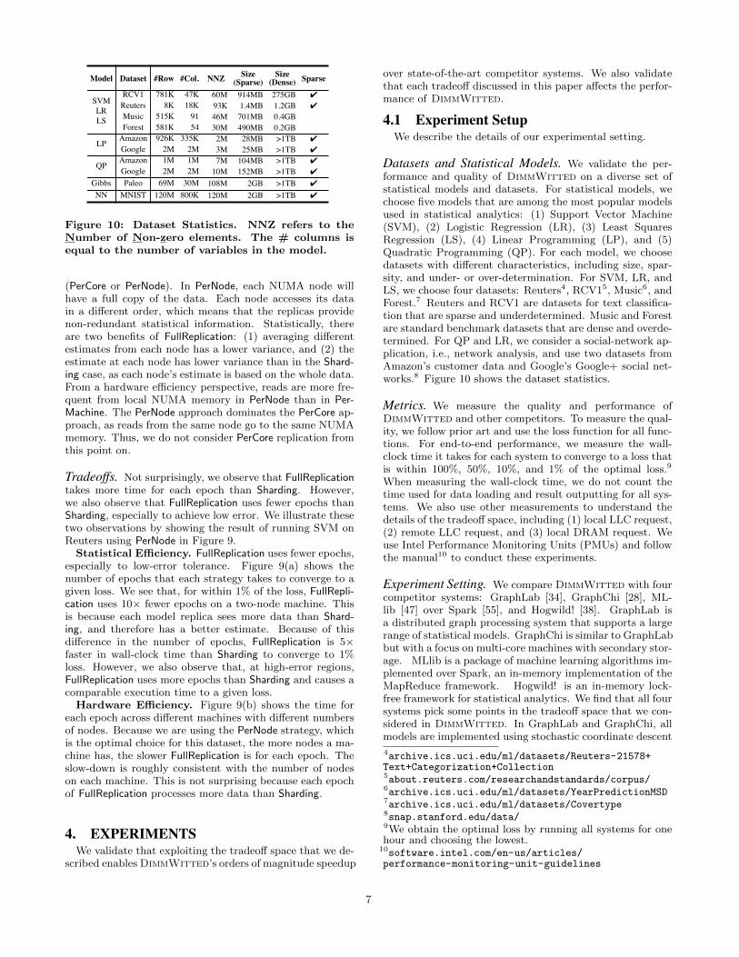
Figure 10: Dataset Statistics. NNZ refers to theNumber of Non-zero elements. The # columns isequal to the number of variables in the model.
(PerCore or PerNode). In PerNode, each NUMA node willhave a full copy of the data. Each node accesses its datain a different order, which means that the replicas providenon-redundant statistical information. Statistically, thereare two benefits of FullReplication: (1) averaging differentestimates from each node has a lower variance, and (2) theestimate at each node has lower variance than in the Shard-ing case, as each node’s estimate is based on the whole data.From a hardware efficiency perspective, reads are more fre-quent from local NUMA memory in PerNode than in Per-Machine. The PerNode approach dominates the PerCore ap-proach, as reads from the same node go to the same NUMAmemory. Thus, we do not consider PerCore replication fromthis point on.
Tradeoffs. Not surprisingly, we observe that FullReplicationtakes more time for each epoch than Sharding. However,we also observe that FullReplication uses fewer epochs thanSharding, especially to achieve low error. We illustrate thesetwo observations by showing the result of running SVM onReuters using PerNode in Figure 9.
Statistical Efficiency. FullReplication uses fewer epochs,especially to low-error tolerance. Figure 9(a) shows thenumber of epochs that each strategy takes to converge to agiven loss. We see that, for within 1% of the loss, FullRepli-cation uses 10× fewer epochs on a two-node machine. Thisis because each model replica sees more data than Shard-ing, and therefore has a better estimate. Because of thisdifference in the number of epochs, FullReplication is 5×faster in wall-clock time than Sharding to converge to 1%loss. However, we also observe that, at high-error regions,FullReplication uses more epochs than Sharding and causes acomparable execution time to a given loss.
Hardware Efficiency. Figure 9(b) shows the time foreach epoch across different machines with different numbersof nodes. Because we are using the PerNode strategy, whichis the optimal choice for this dataset, the more nodes a ma-chine has, the slower FullReplication is for each epoch. Theslow-down is roughly consistent with the number of nodeson each machine. This is not surprising because each epochof FullReplication processes more data than Sharding.
4. EXPERIMENTSWe validate that exploiting the tradeoff space that we de-
scribed enables DimmWitted’s orders of magnitude speedup
over state-of-the-art competitor systems. We also validatethat each tradeoff discussed in this paper affects the perfor-mance of DimmWitted.
4.1 Experiment SetupWe describe the details of our experimental setting.
Datasets and Statistical Models. We validate the per-formance and quality of DimmWitted on a diverse set ofstatistical models and datasets. For statistical models, wechoose five models that are among the most popular modelsused in statistical analytics: (1) Support Vector Machine(SVM), (2) Logistic Regression (LR), (3) Least SquaresRegression (LS), (4) Linear Programming (LP), and (5)Quadratic Programming (QP). For each model, we choosedatasets with different characteristics, including size, spar-sity, and under- or over-determination. For SVM, LR, andLS, we choose four datasets: Reuters4, RCV15, Music6, andForest.7 Reuters and RCV1 are datasets for text classifica-tion that are sparse and underdetermined. Music and Forestare standard benchmark datasets that are dense and overde-termined. For QP and LR, we consider a social-network ap-plication, i.e., network analysis, and use two datasets fromAmazon’s customer data and Google’s Google+ social net-works.8 Figure 10 shows the dataset statistics.
Metrics. We measure the quality and performance ofDimmWitted and other competitors. To measure the qual-ity, we follow prior art and use the loss function for all func-tions. For end-to-end performance, we measure the wall-clock time it takes for each system to converge to a loss thatis within 100%, 50%, 10%, and 1% of the optimal loss.9
When measuring the wall-clock time, we do not count thetime used for data loading and result outputting for all sys-tems. We also use other measurements to understand thedetails of the tradeoff space, including (1) local LLC request,(2) remote LLC request, and (3) local DRAM request. Weuse Intel Performance Monitoring Units (PMUs) and followthe manual10 to conduct these experiments.
Experiment Setting. We compare DimmWitted with fourcompetitor systems: GraphLab [34], GraphChi [28], ML-lib [47] over Spark [55], and Hogwild! [38]. GraphLab isa distributed graph processing system that supports a largerange of statistical models. GraphChi is similar to GraphLabbut with a focus on multi-core machines with secondary stor-age. MLlib is a package of machine learning algorithms im-plemented over Spark, an in-memory implementation of theMapReduce framework. Hogwild! is an in-memory lock-free framework for statistical analytics. We find that all foursystems pick some points in the tradeoff space that we con-sidered in DimmWitted. In GraphLab and GraphChi, allmodels are implemented using stochastic coordinate descent
4archive.ics.uci.edu/ml/datasets/Reuters-21578+Text+Categorization+Collection5about.reuters.com/researchandstandards/corpus/6archive.ics.uci.edu/ml/datasets/YearPredictionMSD7archive.ics.uci.edu/ml/datasets/Covertype8snap.stanford.edu/data/9We obtain the optimal loss by running all systems for onehour and choosing the lowest.
10software.intel.com/en-us/articles/performance-monitoring-unit-guidelines
7

DatasetWithin 1% of the Optimal Loss Within 50% of the Optimal Loss
GraphLab GraphChi MLlib Hogwild! DW GraphLab GraphChi MLlib Hogwild! DW
SVMReuters 58.9 56.7 15.5 0.1 0.1 13.6 11.2 0.6 0.01 0.01RCV1 > 300.0 > 300.0 > 300 61.4 26.8 > 300.0 > 300.0 58.0 0.71 0.17Music > 300.0 > 300.0 156 33.32 23.7 31.2 27.1 7.7 0.17 0.14Forest 16.2 15.8 2.70 0.23 0.01 1.9 1.4 0.15 0.03 0.01
LRReuters 36.3 34.2 19.2 0.1 0.1 13.2 12.5 1.2 0.03 0.03RCV1 > 300.0 > 300.0 > 300.0 38.7 19.8 > 300.0 > 300.0 68.0 0.82 0.20Music > 300.0 > 300.0 > 300.0 35.7 28.6 30.2 28.9 8.9 0.56 0.34Forest 29.2 28.7 3.74 0.29 0.03 2.3 2.5 0.17 0.02 0.01
LSReuters 132.9 121.2 92.5 4.1 3.2 16.3 16.7 1.9 0.17 0.09RCV1 > 300.0 > 300.0 > 300 27.5 10.5 > 300.0 > 300.0 32.0 1.30 0.40Music > 300.0 > 300.0 221 40.1 25.8 > 300.0 > 300.0 11.2 0.78 0.52Forest 25.5 26.5 1.01 0.33 0.02 2.7 2.9 0.15 0.04 0.01
LPAmazon 2.7 2.4 > 120.0 > 120.0 0.94 2.7 2.1 120.0 1.86 0.94Google 13.4 11.9 > 120.0 > 120.0 12.56 2.3 2.0 120.0 3.04 2.02
QPAmazon 6.8 5.7 > 120.0 > 120.0 1.8 6.8 5.7 > 120.0 > 120.00 1.50Google 12.4 10.1 > 120.0 > 120.0 4.3 9.9 8.3 > 120.0 > 120.00 3.70
Figure 11: End-to-End Comparison (time in seconds). The column DW refers to DimmWitted. We take 5runs on local2 and report the average (standard deviation for all numbers < 5% of the mean). Entries with> indicate a timeout.
1
10
100
1000
1% 10% 100%
1
10
100
1000
1% 10% 100%
0.1
1
10
100
1000
1% 10% 100%
0.1
1
10
100
1% 10% 100%
0.01
0.1
1
10
1% 10% 100%
0.01
0.1
1
10
1% 10% 100%
0.1
1
10
100
1% 10% 100%
0.1
1
10
100
1% 10% 100%
SVM (RCV1)
Error to Optimal Loss
Tim
e (s
econ
ds)
(b)
Mod
el R
eplic
atio
n
SVM (Music) LP (Amazon) LP (Google)
PerNode
PerMachine
(a)
Acc
ess M
etho
d Se
l.
Tim
e (s
econ
ds)
Row-wise
Column-wise
PerCore
Figure 12: Tradeoffs in DimmWitted. Missing points timeout in 120 seconds.
(column-wise access); in MLlib and Hogwild!, SVM and LRare implemented using stochastic gradient descent (row-wiseaccess). We use implementations that are provided by theoriginal developers whenever possible. For models with-out code provided by the developers, we only change thecorresponding gradient function.11 For GraphChi, if thecorresponding model is implemented in GraphLab but notGraphChi, we follow GraphLab’s implementation.
We run experiments on a variety of architectures. Thesemachines differ in a range of configurations, including thenumber of NUMA nodes, the size of last-level cache (LLC),and memory bandwidth. See Figure 3 for a summary ofthese machines. DimmWitted, Hogwild!, GraphLab, andGraphChi are implemented using C++, and MLlib/Sparkis implemented using Scala. We tune both GraphLab andMLlib according to their best practice guidelines.12 For both
11For sparse models, we change the dense vector data struc-ture in MLlib to a sparse vector, which only improves itsperformance.
12MLlib:spark.incubator.apache.org/docs/0.6.0/tuning.html; GraphLab: graphlab.org/tutorials-2/fine-tuning-graphlab-performance/. For GraphChi,we tune the memory buffer size to ensure all data fit inmemory and that there are no disk I/Os. We describe moredetailed tuning for MLlib in the full version of this paper.
GraphLab, GraphChi, and MLlib, we try different ways ofincreasing locality on NUMA machines, including trying touse numactl and implementing our own RDD for MLlib;there is more detail in the full version of this paper. Systemsare compiled with g++ 4.7.2 (-O3), Java 1.7, or Scala 2.9.
4.2 End-to-End ComparisonWe validate that DimmWitted outperforms competitor
systems in terms of end-to-end performance and quality.Note that both MLlib and GraphLab have extra overheadfor fault tolerance, distributing work, and task scheduling.Our comparison between DimmWitted and these competi-tors is intended only to demonstrate that existing work forstatistical analytics has not obviated the tradeoffs that westudy here.
Protocol. For each system, we grid search their statisticalparameters, including step size ({100.0,10.0,...,0.0001}) andmini-batch size for MLlib ({1%, 10%, 50%, 100%}); we al-ways report the best configuration, which is essentially thesame for each system. We measure the time it takes for eachsystem to find a solution that is within 1%, 10%, and 50%of the optimal loss. Figure 11 shows the results for 1% and50%; the results for 10% are similar. We report end-to-endnumbers from local2, which has two nodes and 24 logical
8

cores, as GraphLab does not run on machines with morethan 64 logical cores. Figure 14 shows the DimmWitted’schoice of point in the tradeoff space on local2.
As shown in Figure 11, DimmWitted always convergesto the given loss in less time than the other competitors.On SVM and LR, DimmWitted could be up to 10× fasterthan Hogwild!, and more than two orders of magnitudefaster than GraphLab and Spark. The difference betweenDimmWitted and Hogwild! is greater for LP and QP, whereDimmWitted outperforms Hogwild! by more than two or-ders of magnitude. On LP and QP, DimmWitted is also upto 3× faster than GraphLab and GraphChi, and two ordersof magnitude faster than MLlib.
Tradeoff Choices. We dive more deeply into these numbersto substantiate our claim that there are some points in thetradeoff space that are not used by GraphLab, GraphChi,Hogwild!, and MLlib. Each tradeoff selected by our sys-tem is shown in Figure 14. For example, GraphLab andGraphChi uses column-wise access for all models, while ML-lib and Hogwild! use row-wise access for all models and al-low only PerMachine model replication. These special pointswork well for some but not all models. For example, for LPand QP, GraphLab and GraphChi are only 3× slower thanDimmWitted, which chooses column-wise and PerMachine.This factor of 3 is to be expected, as GraphLab also allowsdistributed access and so has additional overhead. Howeverthere are other points: for SVM and LR, DimmWittedoutperforms GraphLab and GraphChi, because the column-wise algorithm implemented by GraphLab and GraphChi isnot as efficient as row-wise on the same dataset. DimmWit-ted outperforms Hogwild! because DimmWitted takes ad-vantage of model replication, while Hogwild! incurs 11×more cross-node DRAM requests than DimmWitted; incontrast, DimmWitted incurs 11× more local DRAM re-quests than Hogwild! does.
For SVM, LR, and LS, we find that DimmWitted out-performs MLlib, primarily due to a different point in thetradeoff space. In particular, MLlib uses batch-gradient-descent with a PerCore implementation, while DimmWitteduses stochastic gradient and PerNode. We find that, for theForest dataset, DimmWitted takes 60× fewer number ofepochs to converge to 1% loss than MLlib. For each epoch,DimmWitted is 4× faster. These two factors contribute tothe 240× speed-up of DimmWitted over MLlib on the For-est dataset (1% loss). MLlib has overhead for scheduling, sowe break down the time that MLlibuses for scheduling andcomputation. We find that, for Forest, out of the total 2.7seconds of execution, MLlib uses 1.8 seconds for computa-tion and 0.9 seconds for scheduling. We also implementeda batch-gradient-descent and PerCore implementation insideDimmWitted to remove these and C++ versus Scala dif-ferences. The 60× difference in the number of epochs untilconvergence still holds, and our implementation is only 3×faster than MLlib. This implies that the main difference be-tween DimmWitted and MLlib is the point in the tradeoffspace—not low-level implementation differences.
For LP and QP, DimmWitted outperforms MLlib andHogwild! because the row-wise access method implementedby these systems is not as efficient as column-wise access onthe same data set. GraphLab does have column-wise access,so DimmWitted outperforms GraphLab and GraphChi be-cause DimmWitted finishes each epoch up to 3× faster,
SVM (RCV1)
LR (RCV1)
LS (RCV1)
LP (Google)
QP (Google)
Parallel Sum
GraphLab 0.2 0.2 0.2 0.2 0.1 0.9 GraphChi 0.3 0.3 0.2 0.2 0.2 1.0 MLlib 0.2 0.2 0.2 0.1 0.02 0.3 Hogwild! 1.3 1.4 1.3 0.3 0.2 13 DIMMWITTED 5.1 5.2 5.2 0.7 1.3 21
Figure 13: Comparison of Throughput(GB/seconds) of Different Systems on local2.
Access Methods Model Replication Data Replication
SVM LR LS
Reuters Row-wise PerNode FullReplication RCV1
Music
LP QP
Amazon Column-wise PerMachine FullReplication Google
Figure 14: Plans that DimmWitted Chooses in theTradeoff Space for Each Dataset on Machine local2.
primarily due to low-level issues. This supports our claimsthat the tradeoff space is interesting for analytic engines andthat no one system has implemented all of them.
Throughput. We compare the throughput of different sys-tems for an extremely simple task: parallel sums. Our im-plementation of parallel sum follows our implementation ofother statistical models (with a trivial update function),and uses all cores on a single machine. Figure 13 showsthe throughput on all systems on different models on onedataset. We see from Figure 13 that DimmWitted achievesthe highest throughput of all the systems. For parallel sum,DimmWitted is 1.6× faster than Hogwild!, and we find thatDimmWitted incurs 8× fewer LLC cache misses than Hog-wild!. Compared with Hogwild!, in which all threads writeto a single copy of the sum result, DimmWitted maintainsone single copy of the sum result per NUMA node, so theworkers on one NUMA node do not invalidate the cacheon another NUMA node. When running on only a singlethread, DimmWitted has the same implementation as Hog-wild!. Compared with GraphLab and GraphChi, DimmWit-ted is 20× faster, likely due to the overhead of GraphLaband GraphChi dynamically scheduling tasks and/or main-taining the graph structure. To compare DimmWitted withMLlib, which is written in Scala, we implemented a Scalaversion, which is 3× slower than C++; this suggests thatthe overhead is not just due to the language. If we do notcount the time that MLlibuses for scheduling and only countthe time of computation, we find that DimmWitted is 15×faster than MLlib.
4.3 Tradeoffs of DimmWitted
We validate that all the tradeoffs described in this paperhave an impact on the efficiency of DimmWitted. We re-port on a more modern architecture, local4 with four NUMAsockets, in this section. We describe how the results changewith different architectures.
4.3.1 Access Method SelectionWe validate that different access methods have different
performance, and that no single access method dominatesthe others. We run DimmWitted on all statistical modelsand compare two strategies, row-wise and column-wise. In
9

0.01
0.1
1
10
100
0.01
0.1
1
10
100 R
atio
of E
xecu
tion
Tim
e pe
r Ep
och
(row
-wise
/col
-wise
)
SVM (RCV1) LP (Amazon)
[e1] [e2] [l2] [l4] [l8] 8x2 8x2 6x2 10x4 8x8
#Cores/Socket ✕ # Sockets [Machine Name] [e1] [e2] [l2] [l4] [l8] 8x2 8x2 6x2 10x4 8x8
Figure 15: Ratio of Execution Time per Epoch (row-wise/column-wise) on Different Architectures. Anumber larger than 1 means that row-wise is slower.l2 means local2, e1 means ec2.1, etc.
each experiment, we force DimmWitted to use the corre-sponding access method, but report the best point for theother tradeoffs. Figure 12(a) shows the results as we mea-sure the time it takes to achieve each loss. The more strin-gent loss requirements (1%) are on the left-hand side. Thehorizontal line segments in the graph indicate that a modelmay reach, say, 50% as quickly (in epochs) as it reaches100%.
We see from Figure 12(a) that the difference between row-wise and column-to-row access could be more than 100×for different models. For SVM on RCV1, row-wise accessconverges at least 4× faster to 10% loss and at least 10×faster to 100% loss. We observe similar phenomena forMusic; compared with RCV1, column-to-row access con-verges to 50% loss and 100% loss at a 10× slower rate.With such datasets, the column-to-row access simply re-quires more reads and writes. This supports the folk wis-dom that gradient methods are preferable to coordinate de-scent methods. On the other hand, for LP, column-wiseaccess dominates: row-wise access does not converge to 1%loss within the timeout period for either Amazon or Google.Column-wise access converges at least 10-100× faster thanrow-wise access to 1% loss. We observe that LR is similarto SVM and QP is similar to LP. Thus, no access methoddominates all the others.
The cost of writing and reading are different and is cap-tured by a parameter that we called α in Section 3.2. We de-scribe the impact of this factor on the relative performanceof row- and column-wise strategies. Figure 15 shows theratio of the time that each strategy uses (row-wise/column-wise) for SVM (RCV1) and LP (Amazon). We see that,as the number of sockets on a machine increases, the ratioof execution time increases, which means that row-wise be-comes slower relative to column-wise, i.e., with increasing α.As the write cost captures the cost of a hardware-resolvedconflict, we see that this constant is likely to grow. Thus,if next-generation architectures increase in the number ofsockets, the cost parameter α and consequently the impor-tance of this tradeoff are likely to grow.
Cost-based Optimizer. We observed that, for all datasets,our cost-based optimizer selects row-wise access for SVM,LR, and LS, and column-wise access for LP and QP. Thesechoices are consistent with what we observed in Figure 12.
4.3.2 Model Replication
We validate that there is no single strategy for model repli-cation that dominates the others. We force DimmWittedto run strategies in PerMachine, PerNode, and PerCore andchoose other tradeoffs by choosing the plan that achievesthe best result. Figure 12(b) shows the results.
We see from Figure 12(b) that the gap between PerMa-chine and PerNode could be up to 100×. We first observethat PerNode dominates PerCore on all datasets. For SVMon RCV1, PerNode converges 10× faster than PerCore to50% loss, and for other models and datasets, we observe asimilar phenomenon. This is due to the low statistical effi-ciency of PerCore, as we discussed in Section 3.3. AlthoughPerCore eliminates write contention inside one NUMA node,this write contention is less critical. For large models andmachines with small caches, we also observe that PerCorecould spill the cache.
These graphs show that neither PerMachine nor PerNodedominates the other across all datasets and statistical mod-els. For SVM on RCV1, PerNode converges 12× faster thanPerMachine to 50% loss. However, for LP on Amazon, Per-Machine is at least 14× faster than PerNode to converge to1% loss. For SVM, PerNode converges faster because it has5× higher throughput than PerMachine, and for LP, PerN-ode is slower because PerMachine takes at least 10× fewerepochs to converge to a small loss. One interesting obser-vation is that, for LP on Amazon, PerMachine and PerNodedo have comparable performance to converge to 10% loss.Compared with the 1% loss case, this implies that PerN-ode’s statistical efficiency decreases as the algorithm tries toachieve a smaller loss. This is not surprising, as one mustreconcile the PerNode estimates.
We observe that the relative performance of PerMachineand PerNode depends on (1) the number of sockets used oneach machine and (2) the sparsity of the update.
To validate (1), we measure the time that PerNode andPerMachine take on SVM (RCV1) to converge to 50%loss on various architectures, and we report the ratio(PerMachine/PerNode) in Figure 16. We see that PerNode’srelative performance improves with the number of sockets.We attribute this to the increased cost of write contentionin PerMachine.
To validate (2), we generate a series of synthetic datasets,each of which subsamples the elements in each row of theMusic dataset; Figure 16(b) shows the results. When thesparsity is 1%, PerMachine outperforms PerNode, as eachupdate touches only one element of the model; thus, thewrite contention in PerMachine is not a bottleneck. As thesparsity increases (i.e., the update becomes denser), we ob-serve that PerNode outperforms PerMachine.
4.3.3 Data ReplicationWe validate the impact of different data replication strate-
gies. We run DimmWitted by fixing data replication strate-gies to FullReplication or Sharding and choosing the best planfor each other tradeoff. We measure the execution time foreach strategy to converge to a given loss for SVM on thesame dataset, RCV1. We report the ratio of these twostrategies as FullReplication/Sharding in Figure 17(a). Wesee that, for the low-error region (e.g., 0.1%), FullReplicationis 1.8-2.5× faster than Sharding. This is because FullReplica-tion decreases the skew of data assignment to each worker,so hence each individual model replica can form a more ac-curate estimate. For the high-error region (e.g., 100%), we
10

0.1
1
10
100
0 0.5 1 0.1
1
10
100
(a) Architecture
#Cores/Socket ✕ # Sockets [Machine Name]
Rat
io o
f Exe
cutio
n Ti
me
(Per
Mac
hine
/Per
Nod
e)
[e1] [e2] [l2] [l4] [l8] 8x2 8x2 6x2 10x4 8x8
(b) Sparsity
Sparsity of Synthetic Data sets on Music
PerMachine Better
PerNode Better
Figure 16: The Impact of Different Architecturesand Sparsity on Model Replication. A ratio largerthan 1 means that PerNode converges faster thanPerMachine to 50% loss.
(b)
1
10
100
Gibbs NN # Va
riab
les/s
econ
d
(Mill
ion)
Classic Choice DimmWitted
0 1 2 3 4 5
0.1% 1.0% 10.0% 100.0%
(a)
Rat
io o
f Exe
c. T
ime
(Ful
lRep
l./Sh
ardi
ng)
FullRepl. Better
Sharding Better
Figure 17: (a) Tradeoffs of Data Replication. A ra-tio smaller than 1 means that FullReplication is faster.(b) Performance of Gibbs Sampling and Neural Net-works Implemented in DimmWitted.
observe that FullReplication appears to be 2-5× slower thanSharding. We find that, for 100% loss, both FullReplicationand Sharding converge in a single epoch, and Sharding maytherefore be preferred, as it examines less data to completethat single epoch. In all of our experiments, FullReplicationis never substantially worse and can be dramatically better.Thus, if there is available memory, the FullReplication datareplication seems to be preferable.
5. EXTENSIONSWe briefly describe how to run Gibbs sampling (which
uses a column-to-row access method) and deep neural net-works (which uses a row access method). Using the sametradeoffs, we achieve a significant increase in speed over theclassical implementation choices of these algorithms. A moredetailed description is in the full version of this paper.
5.1 Gibbs SamplingGibbs sampling is one of the most popular algorithms
to solve statistical inference and learning over probabilis-tic graphical models [43]. We briefly describe Gibbs sam-pling over factor graphs and observe that its main step is acolumn-to-row access. A factor graph can be thought of asa bipartite graph of a set of variables and a set of factors.To run Gibbs sampling, the main operation is to select asingle variable, and calculate the conditional probability ofthis variable, which requires the fetching of all factors thatcontain this variable and all assignments of variables con-nected to these factors. This operation corresponds to thecolumn-to-row access method. Similar to first-order meth-ods, recently, a Hogwild! algorithm for Gibbs was estab-lished [25]. As shown in Figure 17(b), applying the tech-
nique in DimmWitted to Gibbs sampling achieves 4× thethroughput of samples as the PerMachine strategy.
5.2 Deep Neural NetworksNeural networks are one of the most classic machine learn-
ing models [35]; recently, these models have been intensivelyrevisited by adding more layers [19, 29]. A deep neural net-work contains multiple layers, and each layer contains a setof neurons (variables). Different neurons connect with eachother only by links across consecutive layers. The value ofone neuron is a function of all the other neurons in the pre-vious layer and a set of weights. Variables in the last layerhave human labels as training data; the goal of deep neuralnetwork learning is to find the set of weights that maximizesthe likelihood of the human labels. Back-propagation withstochastic gradient descent is the de facto method of opti-mizing a deep neural network.
Following LeCun et al. [30], we implement SGD over aseven-layer neural network with 0.12 billion neurons and 0.8million parameters using a standard handwriting-recognitionbenchmark dataset called MNIST13. Figure 17(b) shows thenumber of variables that are processed by DimmWittedper second. For this application, DimmWitted uses PerN-ode and FullReplication, and the classical choice made by Le-Cun is PerMachine and Sharding. As shown in Figure 17(b),DimmWitted achieves more than an order of magnitudehigher throughput than this classical baseline (to achievethe same quality as reported in this classical paper).
6. RELATED WORKWe review work in four main areas: statistical analytics,
data mining algorithms, shared-memory multiprocessors op-timization, and main-memory databases. We include moreextensive related work in the full version of this paper.
Statistical Analytics. There is a trend to integrate sta-tistical analytics into data processing systems. Databasevendors have recently put out new products in this space, in-cluding Oracle, Pivotal’s MADlib [23], IBM’s SystemML [21],and SAP’s HANA. These systems support statistical analyt-ics in existing data management systems. A key challengefor statistical analytics is performance.
A handful of data processing frameworks have been de-veloped in the last few years to support statistical ana-lytics, including Mahout for Hadoop, MLI for Spark [47],GraphLab [34], and MADLib for PostgreSQL or Green-plum [23]. Although these systems increase the perfor-mance of corresponding statistical analytics tasks signifi-cantly, we observe that each of them implements one pointin DimmWitted’s tradeoff space. DimmWitted is not asystem; our goal is to study this tradeoff space.
Data Mining Algorithms. There is a large body ofdata mining literature regarding how to optimize various al-gorithms to be more architecturally aware [39, 56, 57]. Zakiet al. [39,57] study the performance of a range of different al-gorithms, including associated rule mining and decision treeon shared-memory machines, by improving memory localityand data placement in the granularity of cachelines, and de-creasing the cost of coherent maintenance between multipleCPU caches. Ghoting et al. [20] optimize the cache behaviorof frequent pattern mining using novel cache-conscious tech-niques, including spatial and temporal locality, prefetching,
13yann.lecun.com/exdb/mnist/
11

and tiling. Jin et al. [24] discuss tradeoffs in replication andlocking schemes for K-means, association rule mining, andneural nets. This work considers the hardware efficiency ofthe algorithm, but not statistical efficiency, which is the fo-cus of DimmWitted. In addition, Jin et al. do not considerlock-free execution, a key aspect of this paper.
Shared-memory Multiprocessor Optimization. Per-formance optimization on shared-memory multiprocessorsmachines is a classical topic. Anderson and Lam [4] andCarr et al.’s [14] seminal work used complier techniquesto improve locality on shared-memory multiprocessor ma-chines. DimmWitted’s locality group is inspired by Ander-son and Lam’s discussion of computation decomposition anddata decomposition. These locality groups are the center-piece of the Legion project [6]. In recent years, there havebeen a variety of domain specific languages (DSLs) to helpthe user extract parallelism; two examples of these DSLs in-clude Galois [36, 37] and OptiML [49] for Delite [15]. Ourgoals are orthogonal: these DSLs require knowledge aboutthe trade-offs of the hardware, such as those provided byour study.
Main-memory Databases. The database communityhas recognized that multi-socket, large-memory machineshave changed the data processing landscape, and there hasbeen a flurry of recent work about how to build in-memoryanalytics systems [3,5,16,27,31,40,41,52]. Classical tradeoffshave been revisited on modern architectures to gain signif-icant improvement: Balkesen et al. [5], Albutiu et al. [3],Kim et al. [27], and Li [31] study the tradeoff for joins andshuffling, respectively. This work takes advantage of modernarchitectures, e.g., NUMA and SIMD, to increase memorybandwidth. We study a new tradeoff space for statisticalanalytics in which the performance of the system is affectedby both hardware efficiency and statistical efficiency.
7. CONCLUSIONFor statistical analytics on main-memory, NUMA-aware
machines, we studied tradeoffs in access methods, modelreplication, and data replication. We found that using novelpoints in this tradeoff space can have a substantial bene-fit: our DimmWitted prototype engine can run at leastone popular task at least 100× faster than other competitorsystems. This comparison demonstrates that this tradeoffspace may be interesting for current and next-generationstatistical analytics systems.
Acknowledgments We would like to thank Arun Kumar, Victor
Bittorf, the Delite team, the Advanced Analytics at Oracle, Green-
plum/Pivotal, and Impala’s Cloudera team for sharing their experi-
ences in building analytics systems. We gratefully acknowledge the
support of the Defense Advanced Research Projects Agency (DARPA)
XDATA Program under No. FA8750-12-2-0335 and the DEFT Pro-
gram under No. FA8750-13-2-0039, the National Science Founda-
tion (NSF) CAREER Award under No. IIS-1353606, the Office of
Naval Research (ONR) under awards No. N000141210041 and No.
N000141310129, the Sloan Research Fellowship, American Family In-
surance, Google, and Toshiba. Any opinions, findings, and conclusion
or recommendations expressed in this material are those of the au-
thors and do not necessarily reflect the view of DARPA, NSF, ONR,
or the US government.
8. REFERENCES
[1] A. Agarwal, O. Chapelle, M. Dudık, and J. Langford. A reliableeffective terascale linear learning system. ArXiv e-prints, 2011.
[2] A. Ailamaki, D. J. DeWitt, M. D. Hill, and M. Skounakis.Weaving relations for cache performance. In VLDB, 2001.
[3] M.-C. Albutiu, A. Kemper, and T. Neumann. Massivelyparallel sort-merge joins in main memory multi-core databasesystems. PVLDB, pages 1064–1075, 2012.
[4] J. M. Anderson and M. S. Lam. Global optimizations forparallelism and locality on scalable parallel machines. In PLDI,pages 112–125, 1993.
[5] C. Balkesen and et al. Multi-core, main-memory joins: Sort vs.hash revisited. PVLDB, pages 85–96, 2013.
[6] M. Bauer, S. Treichler, E. Slaughter, and A. Aiken. Legion:expressing locality and independence with logical regions. InSC, page 66, 2012.
[7] N. Bell and M. Garland. Efficient sparse matrix-vectormultiplication on CUDA. Technical report, NVIDIACorporation, 2008.
[8] N. Bell and M. Garland. Implementing sparse matrix-vectormultiplication on throughput-oriented processors. In SC, pages18:1–18:11, 2009.
[9] L. Bergstrom. Measuring NUMA effects with the STREAMbenchmark. ArXiv e-prints, 2011.
[10] C. Boutsidis and et al. Near-optimal coresets for least-squaresregression. IEEE Transactions on Information Theory, 2013.
[11] J. K. Bradley, A. Kyrola, D. Bickson, and C. Guestrin. Parallelcoordinate descent for l1-regularized loss minimization. InICML, pages 321–328, 2011.
[12] G. Buehrer and et al. Toward terabyte pattern mining: Anarchitecture-conscious solution. In PPoPP, pages 2–12, 2007.
[13] G. Buehrer, S. Parthasarathy, and Y.-K. Chen. Adaptiveparallel graph mining for cmp architectures. In ICDM, pages97–106, 2006.
[14] S. Carr, K. S. McKinley, and C.-W. Tseng. Compileroptimizations for improving data locality. In ASPLOS, 1994.
[15] H. Chafi, A. K. Sujeeth, K. J. Brown, H. Lee, A. R. Atreya,and K. Olukotun. A domain-specific approach to heterogeneousparallelism. In PPOPP, pages 35–46, 2011.
[16] C. Chasseur and J. M. Patel. Design and evaluation of storageorganizations for read-optimized main memory databases.PVLDB, pages 1474–1485, 2013.
[17] C. T. Chu and et al. Map-reduce for machine learning onmulticore. In NIPS, pages 281–288, 2006.
[18] E. F. D’Azevedo, M. R. Fahey, and R. T. Mills. Vectorizedsparse matrix multiply for compressed row storage format. InICCS, pages 99–106, 2005.
[19] J. Dean and et al. Large scale distributed deep networks. InNIPS, pages 1232–1240, 2012.
[20] A. Ghoting and et al. Cache-conscious frequent pattern miningon modern and emerging processors. VLDBJ, 2007.
[21] A. Ghoting and et al. SystemML: Declarative machine learningon MapReduce. In ICDE, pages 231–242, 2011.
[22] Y. He and et al. Rcfile: A fast and space-efficient dataplacement structure in mapreduce-based warehouse systems. InICDE, pages 1199–1208, 2011.
[23] J. M. Hellerstein and et al. The MADlib analytics library: OrMAD skills, the SQL. PVLDB, pages 1700–1711, 2012.
[24] R. Jin, G. Yang, and G. Agrawal. Shared memoryparallelization of data mining algorithms: Techniques,programming interface, and performance. TKDE, 2005.
[25] M. J. Johnson, J. Saunderson, and A. S. Willsky. AnalyzingHogwild parallel Gaussian Gibbs sampling. In NIPS, 2013.
[26] M.-Y. Kan and H. O. N. Thi. Fast webpage classification usingurl features. In CIKM, pages 325–326, 2005.
[27] C. Kim and et al. Sort vs. hash revisited: Fast joinimplementation on modern multi-core CPUs. PVLDB, 2009.
[28] A. Kyrola, G. Blelloch, and C. Guestrin. Graphchi: Large-scalegraph computation on just a pc. In OSDI, pages 31–46, 2012.
[29] Q. V. Le and et al. Building high-level features using largescale unsupervised learning. In ICML, pages 8595–8598, 2012.
[30] Y. LeCun and et al. Gradient-based learning applied todocument recognition. IEEE, pages 2278–2324, 1998.
[31] Y. Li and et al. NUMA-aware algorithms: the case of datashuffling. In CIDR, 2013.
[32] J. Liu and et al. An asynchronous parallel stochastic coordinatedescent algorithm. ICML, 2014.
12

[33] Y. Low and et al. Graphlab: A new framework for parallelmachine learning. In UAI, pages 340–349, 2010.
[34] Y. Low and et al. Distributed GraphLab: A framework formachine learning in the cloud. PVLDB, pages 716–727, 2012.
[35] T. M. Mitchell. Machine Learning. McGraw-Hill, USA, 1997.
[36] D. Nguyen, A. Lenharth, and K. Pingali. A lightweightinfrastructure for graph analytics. In SOSP, 2013.
[37] D. Nguyen, A. Lenharth, and K. Pingali. Deterministic Galois:On-demand, portable and parameterless. In ASPLOS, 2014.
[38] F. Niu and et al. Hogwild: A lock-free approach to parallelizingstochastic gradient descent. In NIPS, pages 693–701, 2011.
[39] S. Parthasarathy, M. J. Zaki, M. Ogihara, and W. Li. Paralleldata mining for association rules on shared memory systems.Knowl. Inf. Syst., pages 1–29, 2001.
[40] L. Qiao and et al. Main-memory scan sharing for multi-coreCPUs. PVLDB, pages 610–621, 2008.
[41] V. Raman and et al. DB2 with BLU acceleration: So muchmore than just a column store. PVLDB, pages 1080–1091, 2013.
[42] P. Richtarik and M. Takac. Parallel coordinate descentmethods for big data optimization. ArXiv e-prints, 2012.
[43] C. P. Robert and G. Casella. Monte Carlo Statistical Methods(Springer Texts in Statistics). Springer, USA, 2005.
[44] A. Silberschatz, J. L. Peterson, and P. B. Galvin. OperatingSystem Concepts (3rd Ed.). Addison-Wesley LongmanPublishing Co., Inc., Boston, MA, USA, 1991.
[45] A. Smola and S. Narayanamurthy. An architecture for paralleltopic models. PVLDB, pages 703–710, 2010.
[46] S. Sonnenburg and et al. The SHOGUN machine learningtoolbox. J. Mach. Learn. Res., pages 1799–1802, 2010.
[47] E. Sparks and et al. MLI: An API for distributed machinelearning. In ICDM, pages 1187–1192, 2013.
[48] S. Sridhar and et al. An approximate, efficient LP solver for LProunding. In NIPS, pages 2895–2903, 2013.
[49] A. K. Sujeeth and et al. OptiML: An Implicitly ParallelDomain-Specific Language for Machine Learning. In ICML,pages 609–616, 2011.
[50] S. Tatikonda and S. Parthasarathy. Mining tree-structured dataon multicore systems. PVLDB, pages 694–705, 2009.
[51] J. Tsitsiklis, D. Bertsekas, and M. Athans. Distributedasynchronous deterministic and stochastic gradientoptimization algorithms. IEEE Transactions on AutomaticControl, pages 803–812, 1986.
[52] S. Tu and et al. Speedy transactions in multicore in-memorydatabases. In SOSP, pages 18–32, 2013.
[53] S. Williams and et al. Optimization of sparse matrix-vectormultiplication on emerging multicore platforms. In SC, pages38:1–38:12, 2007.
[54] X. Yang, S. Parthasarathy, and P. Sadayappan. Fast sparsematrix-vector multiplication on gpus: Implications for graphmining. PVLDB, pages 231–242, 2011.
[55] M. Zaharia and et al. Resilient distributed datasets: Afault-tolerant abstraction for in-memory cluster computing. InNSDI, 2012.
[56] M. Zaki, C.-T. Ho, and R. Agrawal. Parallel classification fordata mining on shared-memory multiprocessors. In ICDE,pages 198–205, 1999.
[57] M. J. Zaki, S. Parthasarathy, M. Ogihara, and W. Li. Newalgorithms for fast discovery of association rules. In KDD,pages 283–286, 1997.
[58] M. Zinkevich and et al. Parallelized stochastic gradient descent.In NIPS, pages 2595–2603, 2010.
APPENDIXA. IMPLEMENTATION DETAILS
In DimmWitted, we implement optimizations that arepart of scientific computation and analytics systems. Whilethese optimizations are not new, they are not universallyimplemented in analytics systems. We briefly describes eachoptimization and its impact.
Data and Worker Collocation. We observe that differentstrategies of locating data and workers affect the perfor-mance of DimmWitted. One standard technique is to col-locate the worker and the data on the same NUMA node.In this way, the worker in each node will pull data from itsown DRAM region, and does not need to occupy the node-DRAM bandwidth of other nodes. In DimmWitted, wetried two different placement strategies for data and work-ers. The first protocol, called OS, relies on the operatingsystem to allocate data and threads for workers. The oper-ating system will usually locate data on one single NUMAnode, and worker threads to different NUMA nodes usingheuristics that are not exposed to the user. The second pro-tocol, called NUMA, evenly distributes worker threads acrossNUMA nodes, and for each worker, replicates the data onthe same NUMA node. We find that for SVM on RCV1, thestrategy NUMA can be up to 2× faster than OS. Here aretwo reasons for this improvement. First, by locating dataon the same NUMA node to workers, we achieve 1.24× im-provement on the throughput of reading data. Second, bynot asking the operating system to allocate workers, we ac-tually have a more balanced allocation of workers on NUMAnodes.
Dense and Sparse. For statistical analytics workloads, itis not uncommon for the data matrix A to be sparse, es-pecially for applications such as information extraction andtext mining. In DimmWitted, we implement two protocols,Dense and Sparse, which store the data matrix A as a denseor sparse matrix, respectively. A Dense storage format hastwo advantages: (1) if storing a fully dense vector, it requires12
the space as a sparse representation, and (2) Dense is ableto leverage hardware SIMD instructions, which allows mul-tiple floating point operations to be performed in parallel. ASparse storage format can use a BLAS-style scatter-gatherto incorporate SIMD, which can improve cache performanceand memory throughput; this approach has the additionaloverhead for the gather operation. We find on a syntheticdataset in which we vary the sparsity from 0.01 to 1.0, Densecan be up to 2× faster than Sparse (for sparsity=1.0) whileSparse can be up to 4× faster than Dense (for sparsity=0.01).
The dense vs. sparse tradeoff might change on newerCPUs with VGATHERDPD intrinsic designed to specificallyspeed up the gather operation. However, our current ma-chines do not support this intrinsics and how to optimizesparse and dense computation kernel is orthogonal to themain goals of this paper.
Row-major and Column-major Storage. There are twowell-studied strategies to store a data matrix A: Row-majorand Column-major storage. Not surprisingly, we observedthat choosing an incorrect data storage strategy can causea large slowdown. We conduct a simple experiment wherewe multiply a matrix and a vector using row-access method,
13

where the matrix is stored in column- and row-major order.We find that the Column-major could resulting 9× more L1data load misses than using Row-major for two reasons: (1)our architectures fetch four doubles in a cacheline, only oneof which is useful for the current operation. The prefetcherin Intel machines does not prefetch across page boundaries,and so it is unable to pick up significant portions of thestrided access; (2) On the first access, the Data cache unit(DCU) prefetcher also gets the next cacheline compound-ing the problem, and so it runs 8× slower.14 Therefore,DimmWitted always stores the dataset in a way that isconsistent with the access method—no matter how the in-put data is stored
B. EXTENDED RELATED WORKWe extend the discussion of related work. We summarize
in Figure 18 a range of related data mining work. A keydifference is that DimmWitted considers both hardwareefficiency and statistical efficiency for statistical analyticssolved by first-order methods.
Data Mining Algorithms. Probably the most related workis by Jin et al. [24], who consider how to take advantage ofreplication and different locking-based schemes with differ-ent caching behavior and locking granularity to increase theperformance (hardware efficiency performance) for a rangeof data mining tasks including K-means, frequent patternmining, and neural networks. Ghoting et al. [20] optimizecache-behavior of frequent pattern mining using novel cache-conscious techniques, including spatial and temporal local-ity, prefetching, and tiling. Tatikonda et al. [50] considersimproving the performance of mining tree-structured datamulticore systems by decreasing the spatial and temporallocality, and the technique they use is by careful study of dif-ferent granularity and types of task and data chunking. Chuet al. [17] apply the MapReduce to a large range of statisti-cal analytics tasks that fit into the statistical query model,and implements it on a multicore system and shows almostlinear speed-up to the number of cores. Zaki et al. [56] studyhow to speed up classification tasks using decision trees onSMP machines, and their technique takes advantage dataparallelism and task parallelism with lockings. Buehrer andParthasarathy et al. [13] study how to build a distributedsystem for frequent pattern mining with terabytes of data.Their focus is to minimize the I/O cost and communicationcost by optimizing the data placement and the number ofpasses over the dataset. Buehrer et al. [12] study implement-ing efficient graph mining algorithms over CMP and SMPmachines with the focus on load balance, memory usage (i.e.,size), spatial locality, and the tradeoff of pre-computing andre-computing. Zaki et al. [39,57] study on how to implementparallel associated rule mining algorithms on shared memorysystems by optimizing reference memory locality and dataplacement in the granularity of cachelines. This work alsoconsiders how to minimize the cost of coherent maintenancebetween multiple CPU caches. All of these techniques arerelated and relevant to our work, but none consider optimiz-ing first-order methods and the affect of these optimizationson their efficiency.
14www.intel.com/content/dam/www/public/us/en/documents/manuals/64-ia-32-architectures-optimization-manual.pdf
High Performance Computation. The techniques that weconsidered in DimmWitted for efficient implementation (Sec-tion A) are not new, and they are borrowed from a widerange of literature in high performance computation, database,and systems. Locality is a classical technique: worker anddata collocation technique has been advocated since at least90s [4, 14] and is a common systems design principle [44].
The role of dense and sparse computation is well studiedin the by the HPC community. For example, efficient com-putation kernels for matrix-vector and matrix-matrix mul-tiplication [7,8, 18,53]. In this work, we only require dense-dense and dense-sparse matrix-vector multiplies. There isrecent work on mapping sparse-sparse multiplies to GPUsand SIMD [54], which is useful for other data mining modelsbeyond what we consider here.
The row- vs. column-storage has been intensively studiedby database community over traditional relational database [2]or Hadoop [22]. DimmWitted implements these techniquesto make sure our study of hardware efficiency and statisti-cal efficiency reflects the status of modern hardware, and wehope that future development on these topics can be appliedto DimmWitted.
Domain Specific Languages. Domain specific languages(DSLs) are intended to make it easy for a user to write par-allel programs by exposing domain-specific patterns. Exam-ples of such DSLs include Galois [36, 37] and OptiML [49]for Delite [15]. To be effective, DSLs require the knowl-edge about the trade-off of the target domain to apply theircompilation optimization, and we hope the insights fromDimmWitted can be applied to these DSLs.
Mathematical Optimization. Many statistical analytics tasksare mathematical optimization problems. Recently, the math-ematical optimization community has been looking at howto parallelize optimization problems [32, 38, 58]. For exam-ple, Niu et al. [38] for SGD and Shotgun [11] for SCD. Alock-free asynchronous variant was recently established byJi et al. [32].
C. ADDITIONAL EXPERIMENTS
C.1 More Detailed Tuning Information for SparkWe report details of how we tune our Spark installation
for fair comparison. Figure 19 shows the list of parame-ters that we used to tune Spark. For each combination ofthe parameter, we run one experiment for measuring thethroughput using parallel sum, and use it for all other ex-periments to maximize the performance. For each task, wetry all combinations of step size and batch size.
Statistical Efficiency: Step Size and Batch Size. We ob-serve that step size and batch size of gradient together hassignificant impact on the time that Spark needs to converge.As shown in Figure 19, for each experiment, we try 28 differ-ent combinations of these settings (7 step sizes and 4 batchsizes). We see that these parameters could contribute tomore than 100× in the time to converge to the same losson the same dataset! Therefore, as shown in Figure 19, wetried a large range of these two parameters and pick the bestone to report.
14

Target Architecture Target Application Target EfficiencyMulticore NUMA (SMP) Distributed Data Mining Graph Mining Gradient-based Hardware Statistical
Jin et al. [24] X X X XGhoting et al. [20] X X X
Tatikonda et al. [50] X X XChu et al. [17] X X X XZaki et al. [56] X X X
Buehrer et al. [13] X X XBuehrer et al. [12] X X XZaki et al. [39,57] X X X
Tsitsiklis et al. [51] X XNiu et al. [38] X X X
Bradley et al. [11] X X XGraphChi [28] X X X X X X
GraphLab [33,34] X X X X X XMLlib [47] X X X X X
DimmWitted X X X X
Figure 18: A Taxonomy of Related Work
Type Parameters ValuesStatistical Step size 100, 10, 1, 0.1, 0.01, 0.001, 0.0001Efficiency Batch size 100%, 50%, 10%, 1%
Data Replication 1, 2, 3Serialization True, False
Hardware Storage Level MEMORY ONLYEfficiency Compression True, False
locality.wait 1, 100, 1000, 3000, 10000SPARK MEM 48g, 24g, 1g
numactl localloc, interleave, NA
Figure 19: The Set of Parameters We Tried for Tun-ing Spark
Sources of Overhead in Spark. Spark has overhead inscheduling the task and provide fault tolerance, both ofwhich are features that DimmWitted does not support. Tomake our comparison as fair as possible, we conduct the fol-lowing experiments to understand how scheduling and faulttolerance impact our claims.
We implement our own version of batch-gradient descentalgorithm in DimmWitted by strictly following MLlib’s al-gorithm in C++. On Forest, we first observe that ourown batch-gradient implementation uses similar numbers ofepochs (within 5%) to converge to 1% loss as MLlib given thesame step size and batch size. Second, for each epoch, ourbatch-gradient implementation is 3-7× faster cross differentarchitectures–this implies that MLlib does have overheadcompared with DimmWitted’s framework. However, ourown batch-gradient implementation is still 20-39× slowerthan DimmWitted cross different architectures.
We break down the execution time into the number ofepochs that each system needs to converge and the timethat MLlib used for scheduling and computation. In par-ticular, we use the Forest dataset as an example. On thisdataset, DimmWitted uses 1 epoch to converge to 1% loss,while both MLlib and our own C++ implementation use 63and 64 epochs, respectively. MLlib uses 2.7 seconds for these64 epochs, and 0.9 seconds of these are used for scheduling,and other 1.8 seconds are used to enumerate each example,and calculate the gradient.15 The difference in the numberof epochs to converge implies that the difference betweenMLlib and DimmWitted is not caused by low-level imple-
15 We observe similar break down on other datasets exceptthe smallest dataset, Reuters. On this dataset, the timeused for scheduling is up to 25× of the computation time.
1
3
5
7
9
11
1 3 5 7 9 11
PerCore
PerNode
PerMachine
Delite
# Threads Sp
eedu
p
Linear Speedup
Figure 20: Comparison with Delite using LR (Mu-sic) on local2.
mentations, instead, that MLlib only implements a subsetof points in DimmWitted’s tradeoff space.
Hardware Efficiency. We summarize the impact of param-eters to the throughput of MLlib. For each out of totally 540combinations of all seven parameters related to hardware ef-ficiency, we run the parallel sum to measure the throughput.We find, not surprisingly, that the parameter SPARK MEMhas significant impact on the throughput–On Music, whenthis parameter is set to 48GB, Spark achieves 7× speed-up over 1GB. This is not surprising because this parametersets the amount of RAM that Spark can use. We also findthat, given the SPARK MEM parameter to be 48GB, allother parameters only have less than 50% difference witheach other. Therefore, in our experiments we always useSPARK MEM and set other parameters to be the settingthat achieves highest throughput in our experiment on thecorresponding dataset.
C.2 Comparison with DeliteRecently, there have been a trend of using domain specific
language to help user write parallel programs more easily.We conduct a simple experiment with one popular DSL,namely Delite [15], to illustrate that the tradeoff we studiedin this paper has the potential to help these DSLs to achievehigher performance and quality.
We use the official implementation of logistic regressionin Delite [15] and run both DimmWitted and Delite on theMusic dataset using local2. We try our best effort for the
15

0.1
1
10
100
0.01 0.1 1 Scale (1x = 0.5B rows, 4B NNZs, 49GB)
Tim
e/E
poch
(sec
onds
)
Figure 21: Scalability of DimmWitted usingClueWeb 2009 on local2.
locality of Delite by trying different settings for numactl.We vary the number of threads that each program can useand plot the speed-up curve as shown in Figure 20.
First, we see from Figure 20 that different model replica-tion strategy in DimmWitted has different speed-up behav-ior. Not surprisingly, PerCore speeds up more linearly thanPerNode and PerMachine. These observations are consistentwith the hardware efficiency that we discussed in this paper.More interestingly, we see that Delite does not speed-up be-yond a single socket (i.e., 6 cores). Therefore, by applyingthe PerNode strategy in DimmWitted to Delite, we hopethat we can improve the speed-up behavior of Delite as weillustrated in Figure 20.
C.3 Scalability ExperimentsWe validate the scalability of DimmWitted by testing it
on larger dataset.
Dataset. We follow Kan et al. [26] to create a dataset thatcontains 500 million examples, 100K features for each ex-ample, and 4 billion non-zero elements by using a Web-scaledata set called ClueWeb.16 ClueWeb contains 500 millionWeb pages, and the approach of Kan et al. tries predict thePageRank score of each Web page by using features from itsURLs by a least squares model.
Result. To validate the scalability of DimmWitted, werandomly subsampled 1% examples, 10% examples, and 50%examples to create smaller datasets. We run DimmWit-ted using the rule-of-thumbs in Figure 14, and measure thetime that DimmWitted used for each epoch. Figure 21shows the result. We see that on this dataset, the time thatDimmWitted needs to finish a single epoch grows almostlinearly with the number of examples. We believe that thisis caused by the fact that for all sub-sampled datasets andthe whole dataset, the model (100K weights) fits in the LLCcache.
C.4 Importance Sampling as a Data Replica-tion Strategy
The Sharding and FullReplication sampling scheme that wediscussed in Section 3 assumes that data tuples are equallyimportant. However, in statistic analytics, it is not uncom-mon that some data tuples are more important than others.One example is the linear leverage score.
16http://lemurproject.org/clueweb09/
0.01 0.1 1
10 100
1000
0.01 0.1 1
Importance0.1
Importance0.01
Sharding
FullReplica8on
Time (secon
ds)
Error to Op8mal Loss
Figure 22: Important Sampling on Music (local2).
Example C.1 (Linear Leverage Score [10]). For A ∈RN×d and b ∈ RN . Define s(i) = aTi
(ATA
)−1ai, where ai
is the ith row of A. Let A and b be the result of sampling mrows, where row i is selected with probability proportional tos(i). Then, for all x ∈ Rd, we have
Pr
[∣∣∣∣‖Ax− b‖22 − N
m‖Ax− b‖22
∣∣∣∣ < ε‖Ax− b‖22]>
1
2
So long as m > 2ε−2d log d.
For general loss functions (e.g., logistic loss), the linearleverage score calculated in the same way as above does notnecessarily satisfy the property of approximating the loss.However, we can still use this score as a heuristic to decidethe relative importance of data examples. In DimmWitted,we consider the following protocol that we called Importance.Given a dataset A, we calculate the leverage score s(i) ofthe ith row as aTi (ATA)−1ai. The user specifies the errortolerance ε that is acceptable to her, and for each epoch,DimmWitted samples for each worker 2ε−2d log d exampleswith a probability that is propositional to the leverage score.This procedure is implemented in DimmWitted as one datareplication strategy.
Experimental Results. We run the above importance sam-pling on the same data set as Section 4, and validate thaton some datasets the importance sampling scheme can im-prove the time that DimmWitted needs to converge to agiven loss. Figure 22 shows the results of comparing differ-ent data replication strategies on Music running on local2,where Importance0.1 and Importance0.01 uses 0.1 and 0.01as the error tolerance ε, respectively.
We see that, on Music, Importance0.1 is 3x faster thanFullReplication, for 10% loss. This is caused by the factthat Importance0.1 processes only 10% of the data comparedwith FullReplication. However, Importance0.01 is slowerthan FullReplication. This is because when the error toler-ance is lower, the number of samples one needs to draw foreach epoch increases. For Music, Importance0.01 processesthe same amount of tuples than FullReplication.
D. DETAILED DESCRIPTION OF EXTEN-SIONS
We describe in more details of each extension that wementioned in Section 5.
D.1 Gibbs SamplingFigure 23(a) illustrates a factor graph, which is a bipartite
graph that contains a set of variable, a set of factors, and
16

Variable
Fact
or
Current Variable
Factor
Varia
ble
Current Variable
(a) Factor Graph (b) DimmWitted (c) Deep Neural Networks
Layer 1
Layer 2
Layer n
…
Figure 23: Illustration of Factor Graph and DeepNeural Networks in DimmWitted. (a) and (b) showa factor graph and how DimmWitted represents itas column-to-row access. (c) shows a deep neuralnetwork, and the de facto approach to solve it is torun SGD for each layer DimmWitted in a round-robin fashion.
a set of links between variables and factors. To run Gibbssampling over a factor graph, one processes one variable ata time to calculate the conditional probability for differentassignment of this variable. This involves fetching all con-nected factors and all current assignments of variables thatconnected to these factors. Gibbs sampling then update thecurrent variable assignment by randomly sampling a valueaccording to the conditional probability and proceed to thenext random variable. Similar to first order methods, re-cent theory proves a lock-free protocol to sample multiplevariables at the same time [25]. We also know from classicstatistical theory [43] that one can maintain multiple copy ofthe same factor graph, and aggregate the samples producedon each factor graph at the end of execution.
Figure 23(b) illustrates how DimmWitted models Gibbssampling as column-to-row access. We see that each rowcorresponding to one factor, each column corresponding to
one variable, and the non-zero elements in the matrix cor-respond to the link in the factor graph. To process onevariable, DimmWitted fetches one column of the matrix toget the set of factors, and other columns to get the set ofvariables that connect to the same factor.
In DimmWitted, we implement the PerNode strategy forGibbs sampling by running one independent chain for eachNUMA node. At the end of sampling, we can use all samplesgenerated from each NUMA node for estimation. Therefore,we use throughput, i.e., number of samples generated persecond as the measurement for performance in Section 5.17
In DimmWitted, we implement Gibbs sampling for gen-eral factor graphs, and compare it with one hand-codedimplementation for topic modeling in GraphLab. We runall systems on local2 with 100K documents and 20 topics.We find that on local2, DimmWitted’s implementation is3.7× faster than GraphLab’s implementation without anyapplication-specific optimization.
D.2 Deep Neural NetworksFigure 23(c) illustrates a Deep Neural Network as we de-
scribed in Section 5. Stochastic gradient descent is the defacto algorithm to solve a neural network [30], with one twistthat we will discuss as follows. As shown in Figure 23(c),
17There has been a long historical discussion about the trade-off between a single deep chain and multiple independentchains in statistics. This tradeoff is out of the scope of thispaper.a deep neural network usually contains multiple layers, andthe SGD algorithm needs to be run within each layer, andprocess all layers in a round-robin fashion. Therefore, inDimmWitted, we use the same SGD code path inside eachlayer one at a time, and invoke this code path multiple timesto process different layers.
17