Embed Size (px)
Citation preview

Dimensionality Reduction Techniques for
Modelling Point Spread Functions in
Astronomical Images
Aristos Aristodimou
TH
E
U N I V E R S
I TY
OF
ED I N B U
RG
H
Master of Science
School of Informatics
University of Edinburgh
2011

Abstract
Even though 96% of the Universe is consisted of dark matter and dark energy, their
nature is unknown since modern physics are not adequate to define their characteris-
tics. One new approach that cosmologists are using, tries to define the dark Universe
by precisely measuring the shear effects on galaxy images due to gravitational lensing.
Except the shear effect on the galaxies, there is also another factor that causes distortion
on the images, called the Point Spread Function (PSF). The PSF is caused by atmo-
spheric conditions, imperfections on the telescopes and the pixelisation of the images
when they are digitally stored. This means that before trying to calculate the shear ef-
fect, the PSF must be accurately calculated. This dissertation is part of the GREAT10
star challenge, which is on predicting the PSF on non-star position with high accu-
racy. This work focuses on calculating the PSF at star positions with high accuracy
so that these values can later on be used to interpolate the PSF on non-star positions.
For the purposes of this dissertation, dimensionality reduction techniques are used to
reduce the noise levels in the star images and to accurately capture their PSF. The
techniques used are Principal Component Analysis (PCA), Independent Component
Analysis (ICA) and kernel PCA. Their reconstructed stars are further processed with
the Laplacian of Gaussian edge detection for capturing the boundary of the stars and
removing any noise that is outside this boundary. The combination of these techniques
had promising results in the specific task and outperformed the baseline approaches
that use quadrupole moments.
i

Acknowledgements
I would like to thank my supervisor Dr Amos Storkey for his guidance and for pro-
viding this opportunity to work on this interesting project. Also I would like to thank
Jonathan Millin for all of his comments and help throughout this project.
ii

Declaration
I declare that this thesis was composed by myself, that the work contained herein is
my own except where explicitly stated otherwise in the text, and that this work has not
been submitted for any other degree or professional qualification except as specified.
(Aristos Aristodimou)
iii

Contents
1 Introduction 11.1 Motivation . . . . . . . . . . . . . . . . . . . . . . . . . . . . . . . . 1
1.2 Specific Objectives . . . . . . . . . . . . . . . . . . . . . . . . . . . 2
1.3 Scope of Research . . . . . . . . . . . . . . . . . . . . . . . . . . . . 3
1.4 Contribution . . . . . . . . . . . . . . . . . . . . . . . . . . . . . . . 4
1.5 Thesis Structure . . . . . . . . . . . . . . . . . . . . . . . . . . . . . 4
2 Theoretical Background and Related Work 52.1 Principle Component Analysis . . . . . . . . . . . . . . . . . . . . . 5
2.1.1 Related Work . . . . . . . . . . . . . . . . . . . . . . . . . . 6
2.1.2 Conclusion . . . . . . . . . . . . . . . . . . . . . . . . . . . 6
2.2 Independent Component Analysis . . . . . . . . . . . . . . . . . . . 7
2.2.1 Related Work . . . . . . . . . . . . . . . . . . . . . . . . . . 8
2.2.2 Conclusion . . . . . . . . . . . . . . . . . . . . . . . . . . . 8
2.3 Kernel Principle Component Analysis . . . . . . . . . . . . . . . . . 9
2.3.1 Related Work . . . . . . . . . . . . . . . . . . . . . . . . . . 10
2.3.2 Conclusion . . . . . . . . . . . . . . . . . . . . . . . . . . . 10
2.4 Laplacian of Gaussian Edge Detection . . . . . . . . . . . . . . . . . 10
2.4.1 Conclusion . . . . . . . . . . . . . . . . . . . . . . . . . . . 11
2.5 Quadrupole Moments . . . . . . . . . . . . . . . . . . . . . . . . . . 12
2.5.1 Conclusion . . . . . . . . . . . . . . . . . . . . . . . . . . . 12
3 Data 13
4 Methodology 164.1 Global Evaluation Framework . . . . . . . . . . . . . . . . . . . . . 16
4.2 Local Evaluation Framework . . . . . . . . . . . . . . . . . . . . . . 17
4.3 Baseline Approach . . . . . . . . . . . . . . . . . . . . . . . . . . . 18
iv

4.3.1 Initial baseline approach . . . . . . . . . . . . . . . . . . . . 18
4.3.2 Improved baseline approach . . . . . . . . . . . . . . . . . . 19
4.4 LoG edge detection . . . . . . . . . . . . . . . . . . . . . . . . . . . 19
4.5 PCA . . . . . . . . . . . . . . . . . . . . . . . . . . . . . . . . . . . 20
4.5.1 Component Selection . . . . . . . . . . . . . . . . . . . . . . 21
4.5.2 PCA on each set . . . . . . . . . . . . . . . . . . . . . . . . 23
4.5.3 PCA on each model . . . . . . . . . . . . . . . . . . . . . . 23
4.5.4 PCA on all of the data . . . . . . . . . . . . . . . . . . . . . 25
4.6 ICA . . . . . . . . . . . . . . . . . . . . . . . . . . . . . . . . . . . 25
4.6.1 Component Selection . . . . . . . . . . . . . . . . . . . . . . 26
4.6.2 ICA on each set . . . . . . . . . . . . . . . . . . . . . . . . . 26
4.6.3 Selecting the contrast function . . . . . . . . . . . . . . . . . 27
4.7 Kernel PCA . . . . . . . . . . . . . . . . . . . . . . . . . . . . . . . 28
4.7.1 Component Selection . . . . . . . . . . . . . . . . . . . . . . 28
4.7.2 Kernel PCA on each set . . . . . . . . . . . . . . . . . . . . 28
4.7.3 Kernel Selection . . . . . . . . . . . . . . . . . . . . . . . . 29
5 Results 305.1 RMSE of the noise . . . . . . . . . . . . . . . . . . . . . . . . . . . 30
5.2 Initial baseline approach . . . . . . . . . . . . . . . . . . . . . . . . 31
5.3 Improved Baseline Approach . . . . . . . . . . . . . . . . . . . . . . 33
5.4 PCA . . . . . . . . . . . . . . . . . . . . . . . . . . . . . . . . . . . 35
5.4.1 Component Selection . . . . . . . . . . . . . . . . . . . . . . 35
5.4.2 PCA on each set . . . . . . . . . . . . . . . . . . . . . . . . 37
5.4.3 PCA on each model . . . . . . . . . . . . . . . . . . . . . . 39
5.4.4 PCA on all of the sets . . . . . . . . . . . . . . . . . . . . . 43
5.5 ICA . . . . . . . . . . . . . . . . . . . . . . . . . . . . . . . . . . . 44
5.5.1 Component Selection . . . . . . . . . . . . . . . . . . . . . . 44
5.5.2 Contrast function selection . . . . . . . . . . . . . . . . . . . 47
5.5.3 ICA on each set . . . . . . . . . . . . . . . . . . . . . . . . . 48
5.6 Kernel PCA . . . . . . . . . . . . . . . . . . . . . . . . . . . . . . . 50
5.6.1 Component Selection . . . . . . . . . . . . . . . . . . . . . . 50
5.6.2 Kernel PCA on each set with a RBF kernel . . . . . . . . . . 52
5.6.3 Kernel PCA on each set with a Polynomial kernel . . . . . . . 53
5.7 Comparison of the methods . . . . . . . . . . . . . . . . . . . . . . . 55
v

6 Conclusion 576.1 Future work . . . . . . . . . . . . . . . . . . . . . . . . . . . . . . . 58
Bibliography 59
vi

List of Figures
1.1 The shear and PSF effect on a star and a galaxy . . . . . . . . . . . . 2
3.1 The convolution from telescopic and atmospheric effects . . . . . . . 13
3.2 A star image from each set . . . . . . . . . . . . . . . . . . . . . . . 15
4.1 An example of a Scree plot and the eigenvectors obtained from PCA
on a set . . . . . . . . . . . . . . . . . . . . . . . . . . . . . . . . . 22
4.2 An example of sorted independent components using negentropy . . . 26
5.1 Box-plot of the RMSE on each set using the baseline approach . . . . 32
5.2 An example of a reconstructed star using the baseline approach . . . . 33
5.3 Box-plot of the RMSE on each set using the improved baseline approach 34
5.4 An example of a reconstructed star using the improved baseline approach 35
5.5 Box-plot of the RMSE on each set using PCA on each set . . . . . . . 38
5.6 An example of a reconstructed star using PCA on each set and the LoG
edge detection . . . . . . . . . . . . . . . . . . . . . . . . . . . . . . 39
5.7 The patterns of each model . . . . . . . . . . . . . . . . . . . . . . . 40
5.8 Box-plot of the RMSE on each set using PCA on each model . . . . . 41
5.9 An example of a reconstructed star using PCA on each model and the
LoG edge detection . . . . . . . . . . . . . . . . . . . . . . . . . . . 42
5.10 Box-plot of the RMSE on each set using PCA on all of the sets . . . . 43
5.11 An example of a reconstructed star using PCA on all of the sets and
the LoG edge detection . . . . . . . . . . . . . . . . . . . . . . . . . 44
5.12 Box-plot of the RMSE on the sets ICA was tested using different con-
trast functions . . . . . . . . . . . . . . . . . . . . . . . . . . . . . . 47
5.13 Box-plot of the RMSE on each set using ICA on each set . . . . . . . 48
5.14 An example of a reconstructed star using ICA on each set and the LoG
edge detection . . . . . . . . . . . . . . . . . . . . . . . . . . . . . . 49
vii

5.15 Box-plot of the RMSE on each set using kernel PCA on each set with
the RBF kernel . . . . . . . . . . . . . . . . . . . . . . . . . . . . . 52
5.16 An example of a reconstructed star using PCA on each set and the LoG
edge detection . . . . . . . . . . . . . . . . . . . . . . . . . . . . . . 53
5.17 Box-plot of the RMSE on each set using kernel PCA on each set with
the polynomial kernel . . . . . . . . . . . . . . . . . . . . . . . . . . 54
5.18 An example of a reconstructed star using kernel PCA on each set with
the RBF kernel and the LoG edge detection . . . . . . . . . . . . . . 55
viii

List of Tables
5.1 The mean RMSE of the noise in each set . . . . . . . . . . . . . . . . 31
5.2 The mean RMSE on each set using the baseline approach . . . . . . . 32
5.3 The mean RMSE on each set using the improved baseline approach . 34
5.4 The range of components tested on each PCA method and the selected
number of components . . . . . . . . . . . . . . . . . . . . . . . . . 36
5.5 The mean RMSE on each set using PCA on each set . . . . . . . . . . 38
5.6 The mean RMSE on each set using PCA on each model . . . . . . . . 41
5.7 The mean RMSE on each set using PCA on all of the sets . . . . . . . 43
5.8 The number of components used with each ICA contrast function . . . 46
5.9 The mean RMSE on the sets ICA was tested with each contrast function 47
5.10 The mean RMSE on each set using ICA on each set . . . . . . . . . . 49
5.11 The range of components tested on each Kernel PCA method and the
selected number of components . . . . . . . . . . . . . . . . . . . . . 51
5.12 The mean RMSE on each set using kernel PCA on each set with the
RBF kernel . . . . . . . . . . . . . . . . . . . . . . . . . . . . . . . 52
5.13 The mean RMSE on each set using kernel PCA on each set with the
polynomial kernel . . . . . . . . . . . . . . . . . . . . . . . . . . . . 54
ix

Chapter 1
Introduction
1.1 Motivation
The Universe consists of physical matter and energy, the planets, stars, galaxies, and
the contents of the intergalactic space. The biggest part of the Universe is dark matter
and dark energy whose nature has not yet been fully defined. Because modern physics
are not capable of defining their characteristics, new methods had to be developed.
One promising approach uses the shape distortion of galaxies which is caused by grav-
itational lensing [24]. Gravitational lensing is the effect that light rays are deflected
by gravity. Because there is mass between the galaxies and the observer, images of
galaxies get distorted. This can cause a shear on the galaxy which is a further small
ellipticity on its shape [20]. The cosmologists, by making assumptions of the original
shape of the galaxy, can infer information about the dark matter and dark energy that
is between galaxies and the observer [4].
Except the shear effect, the images are also distorted by a convolution kernel. This
convolution kernel or Point Spread Function (PSF) is caused by a combination of fac-
tors. The first is the refraction of the photons when they travel through our atmosphere.
Then due to slight movements of the telescope or even because the mirrors and lenses
of the telescopes are imperfect and the weight of the mirror warps the mirror differently
at different angles, the image can gets further distortions. Finally, because the images
are digitally stored, there is also a pixelisation which removes some of the detail of the
stars and galaxies and also adds noise to the final image. [20]
Unlike galaxies, stars do not have the shear effect because they are point like ob-
jects. Since stars get distorted only by the PSF, computing the local PSF at a star is
easier than computing it on galaxies. What is needed is to infer the spatially carrying
1

Chapter 1. Introduction 2
PSF at non-star positions using the PSF estimations we have at star positions. By this
we can infer the PSF at a galaxy using the PSF of the stars in its image. Then the
galaxy can be deconvolved using the PSF so that the gravitational lensing can be better
estimated.
An example of the distortion of the stars and galaxies is shown in figure 1.1. In our
data we also expect atmospheric distortions that are caused when the telescopes are not
in space as shown in figure 1.1 but ground-based.
Figure 1.1: The shear effect and PSF effect on stars and galaxies. On the
top pictures a star is seen from a telescope and due to telescope effects
the star is blurred and then due to the detector a pixelated image is created.
For the galaxies there is an additional shear effect caused from the mass
between the galaxy and the observer and then the PSF effect.[20]
1.2 Specific Objectives
This dissertation is part of the GREAT10 star challenge, which is on predicting the PSF
on non-star positions with high accuracy. The interpolation of the PSFs is part of the
dissertations of other students who are participating in the project. This work focuses
on capturing the PSF at star positions with high accuracy. Specifically it focuses on
clearing the star images from the noise so that the star with its PSF can be captured.
This is done using different dimensionality reduction techniques, that help reduce the
noise and also make things easier for the interpolation part. This is because lower
dimensional data need to be interpolated rather than the whole star images. This means
that the optimal number of lower dimensions needs to be defined and then the data need
to be reconstructed so that as much of the noise is removed while the PSF of the star is
unaffected. Due to prediction errors and because the initial components that are used

Chapter 1. Introduction 3
will contain some noise, further noise removal is needed, hence an additional noise
removal technique needs to be used.
1.3 Scope of Research
There are two main ways of finding the PSF, direct modelling and indirect modelling.
Direct modelling uses model fitting whereas indirect modelling uses dimensionality
reduction techniques. For the needs of this dissertation, dimensionality reduction tech-
niques will be used. The assumption is that this approach results in more general
solutions that can be better applied on different data sets. This means that the results
that will be obtained from the artificial data will be close to the results that we would
get using real data. By having more general solutions it also means that no further
adjustments to the technique will be needed when it will be used on real data.
In specific, the dimensionality reduction techniques that will be used are PCA,
ICA and kernel PCA. They will be used on the stars directly as in [18] and then the
reconstructed image from the lower components will have a further noise removal
using the laplacian of Gaussian edge detection. PCA has already been used in different
ways in this area with good results so it should have good results in these data as well.
ICA assumes that the components we are looking for are statistically independent
in our non-Gaussian source [15]. What we have in the star images is a PSF that is
caused by several factors but in the pictures we see all of those factors as a distortion
on the star. If these factors are statistically independent it makes ICA suitable for
this problem. Moreover the fact that the components are independent might help the
interpolation techniques since they will not have to model the dependencies in the
components.
Both of these methods assume that the data lie on a linear subspace which means
that they will not perform well if this is not the case. Kernel PCA is a non-linear
dimensionality reduction technique which will be able to capture any non-linearities
in our data. It has also been proposed in [20] for this task and has been used for
image de-noising in [25]. Another non-linear approach that could be used is Gaussian
Process Latent Variable Models (GP-LVM), but due to time constraints and the size of
the data we have, it was not used after all. Other techniques like ISOMAP and LLE
were considered as well, but there was no clear way of reconstructing the image from
the lower dimensions.

Chapter 1. Introduction 4
1.4 Contribution
As stated earlier, for cosmologists to have good results it is important for them to have
an accurate PSF of the galaxies they are analysing, which is the aim of this project.
By defining the dark Universe with high precision, cosmologists will be able to mea-
sure the expansion rate of the universe, and distinguish between modified gravity and
dark energy explanations for the acceleration of the universe [12]. It will also mark a
revolution in physics, impacting particle physics and cosmology and will require new
physics beyond the standard model of particle physics, general relativity or both.
Moreover, this thesis tests the quality of dimensionality reduction techniques that
have not been used for this task, like ICA and Kernel PCA. Hence the quality of these
new approaches are also presented. The use of edge detection is also tested for further
noise removal on the reconstructed stars from their lower dimensions. This technique
can be used as a post processing step of any other denoising technique for this task.
1.5 Thesis Structure
In Chapter 2 the theoretical background of the techniques used and any related work is
provided, whereas Chapter 3 describes the data used. The next chapter is the method-
ology chapter and explains the way each technique is used to obtain the results on
our data. Then in Chapter 5 the results of each method are reported and discussed.
Finally Chapter 6 provides the conclusion of this dissertation with additional future
work plans.

Chapter 2
Theoretical Background and Related
Work
This chapter provides the theoretical background that is needed for this dissertation.
For each technique that is used, its theory and any related work on identifying the true
PSF of stars in astronomical images is provided. Also a conclusion for each technique
is given that presents the reasons for selecting it for this task.
2.1 Principle Component Analysis
PCA is a popular technique for multivariate statistical analysis and finds application in
many scientific fields [1]. The main goal of PCA is to reduce the dimensionality of the
data from N dimensions to M. This is obtained by transforming the interrelated vari-
ables of the data set to uncorrelated variables, the principal components, in a way that
as much of the variation of the data set is retained. The principal components are or-
dered in a way that the variation explained by each of them is in descending order [19].
This means that the first principal components explain most of the variation in the data
and by using those we can project the data in lower dimensions. It has been shown that
the principal components can be computed by finding the eigenvalues-eigenvectors of
the covariance matrix of the data [19]. Once the eigenvalues-eigenvectors are calcu-
lated, the eigenvectors are sorted in descending order based on their eigenvalues and
then the first M eigenvectors can be used to project the data in lower dimensions. It is
also possible to only calculate the M eigenvalues-eigenvectors using techniques such
as the power method [9]. The original data can be reconstructed from the lower dimen-
sional projections and by using all of the principal components the reconstructed data
5

Chapter 2. Theoretical Background and Related Work 6
will be the same with the initial data set.
Algorithmically PCA on a N-dimensional data set X is as follows:
1. Compute the mean and covariance of X
m =1N
N
∑i=1
xi (2.1)
2. Compute the covariance matrix of X
S =1
N−1
N
∑i=1
(xi−m)(xi−m)T (2.2)
3. Compute the M eigenvectors e1, ...,em with the largest eigenvalues of S and create
the matrix E = [e1, ...em].
4. Project each data point xi to its lower dimensional representation
yi = ET (xi−m) (2.3)
5. If the reconstruction of the original data point xi is needed
xi ≈m+Eyi (2.4)
2.1.1 Related Work
PCA has been used on this task, either directly on the stars [18] or on the estimated
PSF of the stars [30, 17, 26]. In [17] a polynomial fit is first done on the stars and
then PCA is used on those fits. The components of the PCA are later on used for
interpolation. The disadvantage is that this technique depends on the polynomial fit
which as mentioned in [20] it has reduced stability at field edges and corners as the fits
become poorly constrained. As with [17], techniques that try to capture the PSF and
then use PCA to get the components for the interpolation, are dependent on the PSF
fit, which usually is affected by the noise. The authors of [18] use PCA directly on
the stars and by using a lower number of components they reconstruct the image with
lower noise. Then a Lanczos3 drizzling kernel is used to correct geometric distortions.
This approach had better results than wavelet and shapelet techniques but Lanczos3
kernel in some cases produced cosmetic artifacts.
2.1.2 Conclusion
PCA has the advantage of being a powerful and easy to implement technique. Further-
more it has a unique solution and the principal components are ordered, which makes

Chapter 2. Theoretical Background and Related Work 7
the selection of the components easier. The main disadvantage is that it makes the
assumption that data lie on a linear subspace, which is not always the case. PCA has
already been used on the specific task that this thesis is about and had some good re-
sults, which makes it an appropriate technique to be used. What looks promising from
the previous work is [18], because it can be seen as a framework that can be used with
different dimensionality reduction techniques and different methods for removing the
remaining noise.
2.2 Independent Component Analysis
ICA is a non-Gaussian latent variable model that can be used for blind source sepa-
ration. We can see the observed data as being a mixture of independent components,
which leads to the task of finding a way of separating the mixed signals. The ICA
model can be written as
x = As (2.5)
where x is the observed data, A is the mixing matrix and s are the original sources
(independent components). In this model only x is observed whereas A is unknown
and s are the latent variables. To estimate A and s from x, we make the assumption
that the components we are looking for are statistically independent and non-Gaussian
[15].
Once the mixing matrix is estimated, its inverse W is computed so that the inde-
pendent components can be calculated using
s = Wx (2.6)
In [13] a fast and robust method of calculating the independent components is
proposed. This method is known as fast-ICA and is based on maximizing the negative
entropy of the independent components. By normalizing the differential entropy H of
a random vector y = (y1, ...,yn) that has a density f (.) they obtain the negentropy J
which can be used as a nongaussianity measure [8].
H(y) =−∫
f (y) log(y)dy (2.7)
J(y) = H(ygauss)−H(y) (2.8)
where ygauss is a random Gaussian vector that has the same covariance as y.

Chapter 2. Theoretical Background and Related Work 8
Mutual Information is used for measuring the dependence between random vari-
ables and can be expressed using negentropy [8] as :
I(y1, ...,yn) = J(y)−∑i
J(yi) (2.9)
From (2.9) it is easy to see that by maximizing the negentropy the independent com-
ponents get as independent as possible so the task now is maximizing this value. To
approximate the negentropy the following equation is used:
J(yi) = c[EG(yi)−EG(v)]2 (2.10)
where G is a non-quadratic function (contrast function), v is a standardized Gaussian
variable and c is a constant. The contrast functions proposed are:
g1(u) = tanh(a1u) (2.11)
g2(u) = uexp(−a2u2/2) (2.12)
g3(u) = u3 (2.13)
The advantage of this method is that it works with any of these contrast functions
regardless of the distribution of the independent components is. Moreover, by using a
fixed point algorithm the method converges fast and no step size parameters are used
[13].
2.2.1 Related Work
There is no related work on the PSF identification using ICA, but it has been previously
used in image analysis. Specifically in [35] it was used in hyperspectral analysis for
endmember extraction. In this paper ICA was compared to PCA on the task of end-
member extraction and had better results. Also [14] uses ICA to model images that are
noise-free but have the same distribution with the sources of the noisy images. Then
the noisy image is denoised using a maximum likelihood estimation of an ICA model
with noise. The disadvantage is that noiseless images are needed as training sets. It
has also been used in signal processing for clearing a signal from noise. An example is
[22] where ICA is used to remove artifacts from the observed electroencephalographic
signal.
2.2.2 Conclusion
Even though it has not been widely used in image processing, ICA performs really well
in source separation tasks. One of its disadvantages is that the components obtained are

Chapter 2. Theoretical Background and Related Work 9
not ordered, which makes the component selection a bit harder. Another disadvantage
is that as with PCA it is a linear dimensionality reduction technique. The reason that
this method will be used is that our stars are convolved by various factors. If these
factors are considered as statistically independent and nongaussian, then ICA will be
able to separate these factors and by removing the components that represent the noise
in the image, we can get a noiseless image.
2.3 Kernel Principle Component Analysis
This is a non linear version of the PCA which is achieved with the use of kernel func-
tions. The data are first mapped in a feature space F using a non linear function Φ and
then PCA is performed on the mapped data [29]. If our data are mapped in the feature
space and we have (Φ1), ...,(ΦN) then PCA will be on the covariance matrix C
C =1N
N
∑j=1
Φ(x j)Φ(x j)T (2.14)
This means that λV = CV is now transformed to
λ(Φ(xk)V) = Φ(xk)CV (2.15)
with
V =N
∑k=1
akΦ(xk) (2.16)
If a NxN matrix K is defined as
Ki, j = Φ(xi)Φ(x j) (2.17)
then (2.14) and (2.16) can be substituted in (2.15) giving
NλKa = K2a (2.18)
which means that the solutions can be obtained by solving the eigenvalue problem of
Nλa = Ka (2.19)
The solutions of ak are normalized and the components are extracted by calculating
the projections of Φ(x) onto the eigenvectors Vk in feature space F using
(VkΦ(x)) =
N
∑i=1
aki (Φ(xi)Φ(x)) (2.20)

Chapter 2. Theoretical Background and Related Work 10
Because Φ(xi) in (2.17) and (2.20) is not required in any explicit form but only in
dot product, the dot products can be calculated using kernel functions and without
mapping them with Φ [2, 3]. Some kernels that can be used with kernel PCA [29] are
the polynomial and the radial basis functions:
k(x,y) = (x ·yd) (2.21)
k(x,y) = exp(−||x−y||2
2σ2 ) (2.22)
2.3.1 Related Work
As with ICA, there is no related work on the PSF in astronomical images, but it has
been proposed in [20] for this task because of its non linearity. In [25] and [21], the
problem of reconstructing an image from the components is addressed. Also the re-
construction of the image from lower components is being used for noise removal. In
experiments they made, these techniques outperform PCA on the specific task. Specif-
ically [21] has better results than [25] and has also the advantage of being non iterative
and not suffering from local minima. A hybrid approach was later proposed in [31]
which uses [21] to get a starting point for [25] and it has even better results.
2.3.2 Conclusion
The main advantage of Kernel PCA is that it overcomes the problem of the linearity
assumption that PCA and ICA have. Moreover it has been successfully used in image
denoising and was shown to have better results than PCA. These facts and the fact that
it has been proposed in [20], are the main reasons for using it. The disadvantage is that
the reconstruction from the lower dimensions to the initial dimensions is harder than
PCA, but there are techniques for accomplishing that.
2.4 Laplacian of Gaussian Edge Detection
Edges are important changes in an image since they usually occur on the boundary of
different objects in the image [16]. For example in the star images that we have, the
edge might be the stars boundary against the black sky. Edge detection is done by the
use of the first derivative or second derivative operators. First derivative operators like
Prewitt’s operator [27] and Sobel’s operator [10] compute the first derivative and use a
threshold to choose the edges in the image. This threshold may vary in different images

Chapter 2. Theoretical Background and Related Work 11
and noise levels. Second order derivative techniques only select points that have local
maxima by finding the zero crossings of the second derivative of the image [16]. The
disadvantage of second derivative operators is that they are even more susceptible to
noise than first derivative operators.
The Laplacian of Gaussian (LoG) edge detection technique proposed by Marr and
Hildreth [23] first use a Gaussian smoothing filter to reduce the noise and then use a
second derivative operator for the edge detection. The operator used for calculating the
second derivative of the filtered image is the Laplacian operator, which for a function
f(x,y) is
∇2 f =
∂2 f∂x2 +
∂2 f∂y2 (2.23)
The LoG operator’s output is estimated using the following convolution operation
h(x,y) = ∇2[g(x,y) f (x,y)] (2.24)
and by the derivative rule for convolution we have
h(x,y) =[∇
2g(x,y)]
f (x,y) (2.25)
where
∇2g(x,y) =
(x2 + y2−2σ2
σ4
)e−
(x2+y2)2σ2 (2.26)
The LoG edge detection has some good properties [11]. It can be applied in differ-
ent scales so we do not need to know in advance the scale of the interesting features.
Also it is separable and rotation invariant. On the other hand it might detect ’phantom’
edges but this is a general problem with edge detection and post processing techniques
have been introduced to fix these types of problems [7, 6].
2.4.1 Conclusion
No PSF specific related work was done using the LoG technique to be mentioned.
There is a paper in cosmic ray rejection that uses some properties of the LoG but it is
used as a classifier of cosmic rays [34]. The fact that LoG is applicable in different
scales is an important feature, since convolved stars may vary in size and shapes. Also
the fact that it does some images smoothing with a Gaussian filter before actually
detecting the edges might be helpful in our images since they are noisy. This technique
is worth using after reconstructing a star from its lower components for identifying the
star and removing any remaining noise that is not part of the star.

Chapter 2. Theoretical Background and Related Work 12
2.5 Quadrupole Moments
The ellipticity of a star can be measured using the quadrupole moments, but this
method works in the absence of pixelisation, convolution and noise [5]. Initially the
first moments are used to define the centre of the images brightness:
x =∫
I(x,y)xdxdy∫I(x,y)dxdy
(2.27)
y =∫
I(x,y)ydxdy∫I(x,y)dxdy
(2.28)
where I(x,y) is the intensity of the pixel at coordinates x,y. Then the quadrupole
moments can be calculated
Qxx =
∫I(x,y)(x− x)(x− x)dxdy∫
I(x,y)dxdy(2.29)
Qxy =
∫I(x,y)(x− x)(y− y)dxdy∫
I(x,y)dxdy(2.30)
Qyy =
∫I(x,y)(y− y)(y− y)dxdy∫
I(x,y)dxdy(2.31)
and the overall ellipticity of a star can be defined as
ε≡ ε1 + ε2 =Qxx−Qyy +2iQxy
Qxx +Qyy +2(QxxQyy−Qxy2)1/2 (2.32)
If we have an elliptical star with a major axis a and minor axis b and the angle between
the positive x axis and the major axis was θ then [5]
ε1 =a−ba+b
cos(2θ) (2.33)
ε2 =a−ba+b
sin(2θ) (2.34)
2.5.1 Conclusion
The quadrupole moments do not take into consideration the noise and pixelisation
so they will not work well on the initial images. Once the noise is removed from the
image, they can be used as the covariance matrix of a Gaussian, centred on the location
of the star in the image. By this a star can be recreated using the quadrupole moments.
The covariance matrix S will be
S =
(Qxx Qxy
Qxy Qyy
)(2.35)

Chapter 3
Data
The data used are from the GREAT10 star challenge [20]. The data are artificially
generated illustrating the real PSF effects on star images. The PSF is caused by atmo-
spheric and telescopic effects and further noise and pixelisation is added to the image
due to the detectors. An example of the atmospheric and telescopic effects can be seen
in figure 3.1.
Figure 3.1: The upper panel shows the real point like stars and the resulted
observed stars due to the atmospheric and telescopic effects.
The lower panel shows the atmospheric convolution on the left, and the tele-
scopic convolution on the right. The atmospheric convolution has random,
coherent patterns, whereas the telescopic convolution has specific functional
behaviour due to optical effects
The data set is approximately 50GB and contains 26 sets with 50 images in each
13

Chapter 3. Data 14
set. Each image has 500 to 2000 stars depending on the set it belongs to. There are
approximately 1.3 million stars to be analysed and each star is in a 48x48 pixel patch
in the image. To reduce the size of the files more, the stars were extracted from the
images and the patches size was reduced to 30x30 pixel. This reduced the size of the
data set to approximately 9Gb so that each set can be processed by a typical 64bit
personal computer.
To artificially create the star data, a PSF convolution is done on point like stars.
In each set, the images were created with the same underlying PSF, but they illustrate
different gravitational lensing effects by using different random components. Further-
more, the PSF varies spatially across an image so that stars in the same image have
different convolutions. After the PSF convolution, the pixelisation effect is created by
summing the star intensities in square pixels. Finally, noise is added to the images.
The noise added is uncorrelated Gaussian and the image simulation process also adds
Poisson noise.
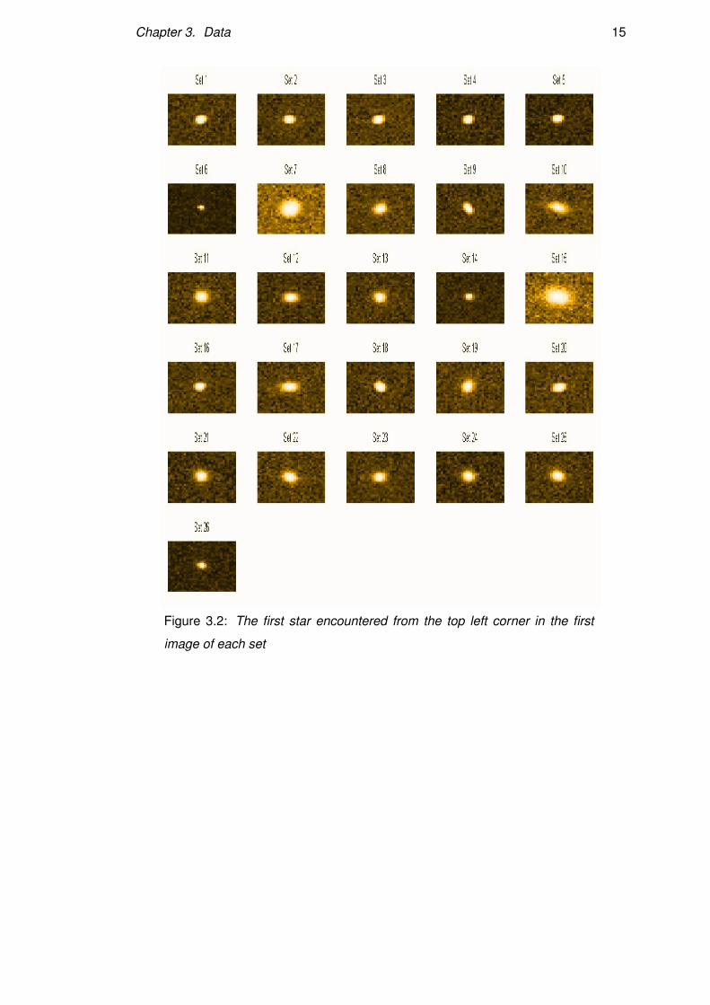
An example of a star from each set is shown in figure 3.2. Specifically, this is the
first star encountered in the first image of each set. As can be seen, the PSF is varying
giving different convolution to the stars in each set. This is affecting the elliptical
shape and size of the observed stars. For example in sets 6, 14 and 26 the observed
stars are much smaller, whereas is sets 7 and 15 the observed stars are larger. Because
of this variation of shapes and sizes, the techniques used must be able to take them into
account to have good results.
Chapter 3. Data 15
Figure 3.2: The first star encountered from the top left corner in the first
image of each set
Chapter 4
Methodology
This chapter presents the way each method is used and the way the experiments are
performed. First a global evaluation framework is provided for evaluating the different
dimensionality reduction techniques using the competition’s evaluation method. Also
a local evaluation framework is shown that can be used for locally optimizing the
techniques before using the global evaluation framework. Then a baseline approach
and its evaluation is presented. Finally the algorithms for optimizing and running the
different techniques are provided.
4.1 Global Evaluation Framework
The main purpose of this dissertation is to use different dimensionality reduction tech-
niques in order to capture the PSF of the stars. This can be done by projecting the
data into lower components that are explaining the structure of the PSF and not the
noise. This means that the reconstructed stars from their lower components will have
less noise. These lower dimensional data can be used for interpolating the PSF at non-
star positions in the images. This makes the interpolation easier, since now it will not
be necessary to interpolate the whole star image. Once the predicted components are
estimated, the stars with their PSF can be reconstructed. Due to prediction errors and
because the initial components that are used for training will contain some noise, fur-
ther noise removal is needed. For this task, LoG edge detection will be used. Edge
detection will capture the boundary of a star and therefore, any noise that is outside the
boundary of a star can be removed. The final star images can be evaluated by upload-
ing them to the GREAT10 star challenge website, which will provide a quality factor
for the submitted data. All of the above provide the following global framework for
16

Chapter 4. Methodology 17
evaluating the results of different dimensionality reduction techniques.
Global Evaluation Framework
1. Use a dimensionality reduction technique to project the training data
to lower dimensions
2. Provide the lower dimensional data for interpolation on the asked
non-star positions
3. Reconstruct the stars from the predicted values
4. Use LoG edge detection to remove any noise outside the stars’ boundaries
5. Submit the final stars to the competition’s website for evaluation
This framework will be used once the values at the non-star positions are predicted
using the data provided by this dissertation. Because this means that work from differ-
ent dissertations needs to be combined, it will be used in a future stage.
4.2 Local Evaluation Framework
Because the data to be submitted will be gigabytes in size and only one submission
per day is allowed, the global evaluation framework is to be used when all of the local
optimizations of the methods are done. Since the global evaluation framework is not
suitable for optimizing the methods used, a local evaluation framework is needed. This
means that the methods can be tested only using the noisy star images. First, the data
are projected to their lower dimensions using a dimensionality reduction technique.
Then the stars are reconstructed from the lower dimensions and any remaining noise
is removed using LoG edge detection. To evaluate the final star images, the root mean
square error (RMSE) is calculated between the final star images and the original noisy
star images. The RMSE for two vectors x1 and x2 is
RMSE =
√√√√ n∑
i=1(x1,i−x2,i)
2
n(4.1)
Because the star pixels usually have larger intensities than the pixels that just have
noise, this evaluation can tell us how good the noise removal was. If the noise removal
is perfect, then the RMSE will account only for the noisy pixels. Since the noise inten-
sities are small the RMSE value will be small. In case we were not able to reconstruct

Chapter 4. Methodology 18
the star with its true PSF, then the error will be larger. For example if the star was el-
liptical but instead a spherical star was created, then noise pixels will be tested against
star pixels and vice versa, hence the RMSE will be larger. If the RMSE is 0 then it
means that no change to the noisy image was done,therefore the technique failed. The
local evaluation framework is the following.
Local Evaluation Framework
1. Use a dimensionality reduction technique to project the training data
to lower dimensions (different parameters can be used to optimize the
technique)
2. Reconstruct the stars from their lower dimensions
3. Use LoG edge detection to remove any noise outside the stars’ boundaries
4. Calculate the error between the noisy and final star image using (4.1)
This framework will be used for testing different number of components on different
dimensionality reduction techniques using different contrast functions or kernels. Be-
cause this will require a dissent amount of time, the evaluation is done on a subset of
the data (approximately 10%). Specifically it is using 100 randomly chosen stars from
each image of each set, which were chosen once and used for all of the optimizations of
the dimensionality reduction techniques. When the optimizations are done for a tech-
nique, then the local evaluation technique is run on all of the data so that a comparison
between different techniques can be made.
4.3 Baseline Approach
4.3.1 Initial baseline approach
As baseline, the ellipticity of the stars is calculated using the quadrupole moments
(2.27-2.31). The quadrupole moments are calculated using the noisy star images. Then
each star is recreated using a Gaussian with a covariance function like (2.35) and cen-
tred at the stars’ location. The algorithm of the baseline approach is the following:
Chapter 4. Methodology 19
Algorithm 4.1 Baseline approach
1. Calculate the centre of the image brightness using (2.27) and (2.28)
2. Calculate the quadrupole moments of a star using (2.29-2.31)
3. Recreate a star using a Gaussian with a covariance matrix as (2.35)
and centred at the star location
4. Calculate the RMSE between the noisy star and the recreated star using (4.1)
4.3.2 Improved baseline approach
The initial baseline approach can be further improved by trying to remove the noise
with dimensionality reduction techniques. Specifically, a preprocessing of the data
using PCA is done to see how much the baseline approach is improve when noise is
removed. These results are then compared with the initial baseline approach and the
local evaluation framework that uses edge detection instead of quadrupole moments.
The problem encountered with the quadrupole moments approach, is that there are
cases that their values cannot be used as a covariance of a Gaussian. This means that
there are cases where stars cannot be reconstructed. In these cases, in the improved
baseline approach the preprocessed star with PCA was used as the reconstructed star
instead. In the initial baseline approach those stars had to be ignored.
4.4 LoG edge detection
The LoG edge detection is provided as a built in function in MATLAB and it is used
for the purposes of this dissertation. The function is used with a threshold equal to
zero so that all zero crossing are marked as edges, which results in returning edges that
are in closed contour form. What is actually returned by the function is a matrix of the
same size of the input matrix, which in this case is a 30x30 matrix. The returned matrix
has all its values set to 0 except the pixels that denote the edges, which are set to 1.
There are cases where some of the noise outside the boundary of the star is set as extra
edge. Because these pixels are outside the boundary of the star they can be ignored
by using the first contour that we encounter from the central pixel of the image. To
remove any noise outside the boundary of the star the pixels inside the boundary are
set to 1, whereas the rest are set to 0. This matrix can be used as a mask for removing
the remaining noise. If the star image was X and the mask is Y then the cleaned star

Chapter 4. Methodology 20
image C is obtained using
Ci, j = Xi, jYi, j (4.2)
The algorithm for removing the noise outside the boundary of the star is the following:
Algorithm 4.2 Remove the remaining noise of the reconstructed star
1. Y = edge(X,’log’,0)
2. From centre pixel of Y move upwards until a pixel with the value 1 is found
3. Mark pixel as visited
4. Check clockwise from that pixel for a pixel with the value 1 that is not visited
5. Repeat from step 3 until all neighbouring pixels with value 1 are visited.
6. Reset all the pixels of Y to zero except the ones that are marked as visited
7. Set all pixels inside this new boundary in Y to 1
8. Clear the remaining noise using (4.2)
4.5 PCA
This is the first method to be used and will provide data for other students who are
working with the interpolation task of this project. Because different approaches will
be used for the interpolation, some students might use stars from the images of all the
sets as their training sets whereas others will use star images from one set at a time or
even stars from a single image. This means that each approach will need its training
data to be in the same dimensionality. For example, if only stars from a single image
are used, then each image might have a different number of principal components, but
the stars in an image must all be reduced to the same dimensionality. On the other
hand, if all of the images from all the sets are used as training data, then all of the stars
must be reduced to the same dimensionality. A single representation could be used by
using all of the data as training set so that all of the stars are reduced to the same dimen-
sionality, but as will be seen in the results chapter, the number of principal components
needed is much greater. This would make the interpolation slower for approaches were
all of these information is not needed. Taking the above into consideration, it was de-
cided to create a representation on each set separately, a representation on all of the
sets and if any patterns are noticed on the principal components on each set, make a
representation on sets with the same patterns.

Chapter 4. Methodology 21
4.5.1 Component Selection
The number of components to be used affects the quality of the recreated star images,
hence the quality of PCA is affected. To get the best possible number of components,
a range of different number of components is tested. That is because there is no clear
way of selecting the number of components without any uncertainty. The lower bound
of the range is the number of components that we get using the Scree test and the upper
bound is the number of components that visually have an apparent structure and are
not overfitting the data. To check whether the components to be tested are overfitting
the data or not, the structural information that is known for each star patch is used. The
information is that the corners of each star patch are just noise. All the noise terms are
combined together for all the stars in the image and their variance is estimated using
Var(X) = E[(X−µ)2
](4.3)
Then the assumption that variance is stationary across the image is made. Once the data
are reconstructed from their lower dimensions, the reconstructed image is subtracted
from the original. If the components are not overfitting, then the residual will contain
at least the noise and maybe some star structure as well. In this case, the variance of
the residual will be larger or equal to the variance of the noise. If this is not the case,
then the components contain noise and are overfitting. This is checked for a range
of number of components, which has as a lower bound the number of components
obtained from the Scree test and as an upper bound the number of components that
visually have apparent structure.
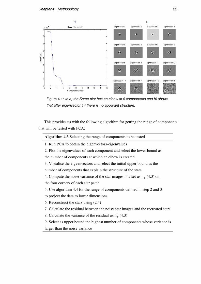
In figure 4.1 an example of a Scree plot and the eigenvectors obtained with PCA
on set 1 of the data is shown. From the Scree plot it is obvious that there is an elbow at
component 6, since after that point the line levels off. From the eigenvectors images, it
can be seen that eigenvectors 1 to 14 have some structure, whereas after eigenvector 14
the structure is lost. We assume that in this case any eigenvector after the 14th captures
the noise and not the stars. Hence, the components to be checked for overfitting are
components 6 to 14 using the variance of the noise. Once the highest number of non
overfitting components is calculated, it will be used as the upper bound of number of
components that PCA will be tested using the local evaluation framework. The number
of components with the lowest RMSE will be selected as the number of components
to be used from projecting that set to lower dimensions.
Chapter 4. Methodology 22
Figure 4.1: In a) the Scree plot has an elbow at 6 components and b) shows
that after eigenvector 14 there is no apparant structure.
This provides us with the following algorithm for getting the range of components
that will be tested with PCA:
Algorithm 4.3 Selecting the range of components to be tested
1. Run PCA to obtain the eigenvectors-eigenvalues
2. Plot the eigenvalues of each component and select the lower bound as
the number of components at which an elbow is created
3. Visualise the eigvenvectors and select the initial upper bound as the
number of components that explain the structure of the stars
4. Compute the noise variance of the star images in a set using (4.3) on
the four corners of each star patch
5. Use algorithm 4.4 for the range of components defined in step 2 and 3
to project the data to lower dimensions
6. Reconstruct the stars using (2.4)
7. Calculate the residual between the noisy star images and the recreated stars
8. Calculate the variance of the residual using (4.3)
9. Select as upper bound the highest number of components whose variance is
larger than the noise variance
Chapter 4. Methodology 23
4.5.2 PCA on each set
Since only a single set will be loaded every time in memory for this task, no further
changes need to be done on the standard PCA. As the stars are in 30x30 pixel patches,
they have to be converted to vectors so that the training data are a 900xK dimensions,
where K is the number of stars in the set. This will be referred to as the vectorisation
of the data.
To project the data to lower dimensions, the following algorithm is run on each set:
Algorithm 4.4 PCA on each set
1. Vectorise the set
2. Get the mean m using (2.1)
3. Calculate the covariance matrix S using (2.2)
4. Perform the eigenvector-eigenvalue decomposition
5. Sort the eigenvectors in descending order based on their eigenvalues
6. Select the number of components to be used
7. Project the data to lower dimensions using (2.3)
This algorithm is run on the different number of components that are obtained using
algorithm 4.3 for optimization. For each lower dimensional representation that is ob-
tained, the local evaluation framework is used on a subset of stars of that set to get the
RMSE using that number of components. The reconstruction of the data from their
lower dimensions is done using (2.4).
4.5.3 PCA on each model
For doing PCA on sets with similar patterns, first the eigenvectors obtained from doing
PCA on each set need to be examined by hand. Any sets with similar patterns need to
be combined together to be used as single training set for PCA. This is because these
sets will be considered to be created using a similar model, which might represent a
certain type of telescopic or atmospheric effects. Due to this, the lower dimensional
data obtained can be used by the students who are taking into consideration these ef-
fects when doing interpolation. Only one set can be loaded in memory, due to memory
limitations of the computers available, hence a different approach needs to be used.
Specifically, instead of using all of the sets of a model for calculating the covariance
matrix, the average covariance matrix can be used. What is needed is to calculate

Chapter 4. Methodology 24
the covariance matrix and mean of these sets and then use the average of them for
the eigenvector-eigenvalue decomposition and for the reconstruction from the lower
dimensions. This leads to the following algorithm:
Algorithm 4.5 PCA on each model
1.1 for each set i that belongs to a certain model
1.2 Vectorise the set
1.3 Get the mean mi using (2.1)
1.4 Calculate the covariance matrix Si using (2.2)
1.5 end2. Get the average covariance matrix S and the average mean mfrom all Si and mi respectively
3. Perform the eigenvector-eigenvalue decomposition on S4. Sort the eigenvectors in descending order based on their eigenvalues
5. Select the number of components to be used
6. Project the data to lower dimensions using (2.3) with m
For selecting the optimal number of components in this case, the steps for evaluating
the different number of components are the same as in PCA on each set. The difference
is that now the number of components selected must have the lowest mean RMSE on all
of the sets of the model that is being tested. Now consider the case where a set needs
at least 20 components to recreate the stars without loosing their original ellipticity.
If another set that belongs to this same model has as an upper bound on the range of
components to be selected was 15 components, then this number of components cannot
be selected for all of the sets of that model. If the highest upper bound of all the sets is
used as the upper bound for all the sets of that model then this problem is solved. The
disadvantage is that any set that had less components as its upper bound will be slightly
overfitted to the data, but this is preferred than having sets whose recreated stars are
wrong. Because pixel intensities vary from set to set, the error will vary as well, so
using the mean directly is not the best choice. What is done instead, is to divide the
RMSEs of each set with the maximum RMSE of that set. For example, if in set 1 the
maximum RMSE was with 10 components then the RMSE obtained by using different
number of components on set 1, will be divided by the RMSE of the 10 components.
This way, the number of components that gave the maximum RMSE will be equal to
1 and the rest will be less than 1 according to how much smaller their RMSE was.

Chapter 4. Methodology 25
Now the mean of these values can be used and the number of components that has the
smallest mean RMSE is selected as the optimal number of components for that model.
For the reconstruction of the data from their lower dimensions (2.4) is used, where mis the average mean of the model obtained from algorithm 4.5.
4.5.4 PCA on all of the data
This task is the same as doing PCA on each model but in this case all of the sets belong
to the same model. So the algorithm is:
Algorithm 4.6 PCA on all of the data
1.1 for each set i
1.2 Vectorise the set
1.3 Get the mean mi using (2.1)
1.4 Calculate the covariance matrix Si using (2.2)
1.5 end2. Get the average covariance matrix S and the average mean mfrom all Si and mi respectively
3. Perform the eigenvector-eigenvalue decomposition on S4. Sort the eigenvectors in descending order based on their eigenvalues
5. Select the number of components to be used
6. Project the data to lower dimensions using (2.3) with m
To select the optimal number of components the same procedure with the PCA on
each model is used, with the difference that now the reconstruction uses the average
mean of all the sets.
4.6 ICA
The denoising of the stars is done using the Denoising Source Seperation (DSS) tool-
box for MATLAB proposed in [28], which provides a framework for applying different
denoising functions based on blind source separation. Specifically fast-ICA with dif-
ferent contrast functions is used for this dissertation.

Chapter 4. Methodology 26
4.6.1 Component Selection
The application used for ICA sorts the returned components using their negentropy,
providing a higher significance to the first components, which will make easier the
selection of the components to be used. Even though the components are sorted, there
are cases where a component less structure explanation and more noise has a better
ranking than a component with less noise. An example is shown in figure 4.2 where
component 8 is better ranked than component 9 while it is more noisy.
Figure 4.2: The first 10 independent components of set 1 sorted with negen-
tropy. Component 8 has a better ranking than component 9 while it is clear
that this is not the case.
Even though negentropy gives a better ranking to components with some structure
compared to unstructured components, the ranking between structured components is
not the optimal. This means that the approach of selecting the number of components
using a range of different number of components as in PCA is not appropriate in this
case. A better approach would probably be the use of a genetic algorithm for selecting
the best structured components, but due to time limitations this was not used. Instead,
all of the components that represent some structure of the stars were selected by hand.
4.6.2 ICA on each set
ICA is tested only using each set as training set, because the results will be available
much sooner than running it on each model and all of the sets. The main idea is that
these results will be compared with the PCA results and if the RMSE is better then
it can be run on each model and all of the sets at a future time. Also to do that, the

Chapter 4. Methodology 27
interpolation obtained by the methods using the data from all the sets or each model
need to be better than the interpolation used on each set separately.
Because ICA can get stuck in local minima, it needs to be run more than once on
each set. In the experiments performed, ICA was run 10 times on each set. For each
run the RMSE is calculated using the local evaluation framework and the independent
components from the run with the lowest RMSE are used as the optimized independent
components. The algorithm for performing ICA on a set is the following:
Algorithm 4.7 ICA on each set
1. Vectorise the set
2.1 for i = 1 to N
2.2 Perform ICA using the DSS toolbox with the selected contrast function
2.3 Select the independent components to be used
2.4 Store the mixing matrix Ai and the unmixing matrix Wi of those components
2.5 end
Once the mixing and unmixing matrices of each run are computed, they can be used
in the local evaluation framework to get the RMSE of each run. For projecting the data
to lower dimensions (2.6) is used and for reconstructing them from lower dimension
(2.5). The selected mixing and unmixing matrices are the ones that produced the lowest
RMSE.
4.6.3 Selecting the contrast function
As mentioned in [13] ICA can be optimized using different contrast functions. The
contrast functions used for optimizing ICA as proposed in [13] are the tanh (2.11),
gauss (2.12) and kurtosis (2.13) functions shown in Chapter 2. To compare the contrast
functions, algorithm 4.7 is used on different sets using each contrast function to obtain
the best mixing and unmixing matrices using the local evaluation framework. This was
done on 7 of the 26 sets, which were chosen so that at least 2 sets from each model
found with PCA are in the training sets. Moreover they were selected so that there will
exist at least one set from the sets with the smaller stars and one set from the sets with
the larger stars. Once the RMSEs using each contrast function are obtained, their mean
RMSEs on each set and the variation fo the RMSEs are compared to decide which a
contrast function gives the best results.

Chapter 4. Methodology 28
4.7 Kernel PCA
The function kernelPCA of the DR Toolbox [33] in MATLAB is used for the denoising
of the stars. This implementation allows the use of a polynomial kernel (2.21) and a
radial basis function kernel (RBF) (2.22). Both of these kernels are tested so that the
optimal can be found.
4.7.1 Component Selection
Kernel PCA first maps the data to a feature space F using a non linear function Φ and
then PCA is performed on the mapped data. This means that the final results will be the
eigenvectors and eigenvalues from PCA on the mapped data. Hence the eigenvectors
will be sorted in descending order based on their eigenvalues. For these reasons, the
process of selecting the components is the same with PCA with the exception that
in step 1 and 5 of algorithm 4.3 kernel PCA will be used instead of PCA. Also the
reconstruction at step 6 is done using (4.4).
4.7.2 Kernel PCA on each set
As with ICA, kernel PCA is tested only using each set as training set. In contrast to
ICA kernel PCA on a set has a unique solution [32], which means that it will only
be run once on each set with a certain kernel function. The algorithm for performing
kernel PCA on a set is the following:
Algorithm 4.8 Kernel PCA on each set
1. Vectorise the set
2. Perform kernel PCA using the DR toolbox with the selected kernel function
3. Select the principal components to be used
4. Project the data to lower dimensions using the eigenvectors E with the
equation y = ET x
This can be used as step 1 of the local evaluation framework so that the RMSE can
be calculated. For the reconstruction of the data from their lower dimensions, there
wasn’t time to implement one of the algorithms proposed in [25] and [21], so a simple
and naive solution is used. The inverse of the eigenvectors returned from kernel PCA
is used, so the reconstruction of the data is done using
x = (ET )−1y (4.4)

Chapter 4. Methodology 29
4.7.3 Kernel Selection
Kernel PCA is tested using the polynomial and radial basis function (RBF) kernel
introduced in Chapter 2. The polynomial kernel is using a fourth order polynomial
because it was found to remove most of the noise when the star images were visual-
ized. To compare the effects of each kernel, algorithm 4.8 is used on each set using
each kernel function after the optimal number of components is calculated using the
component selection algorithm. Once the RMSEs using each kernel are obtained, their
mean RMSEs on each set and the variation fo the RMSEs are compared to decide
whether a kernel can be selected as the optimal.

Chapter 5
Results
In this chapter, the results of the experiments are presented and discussed. For each
approach used, a box-plot of the RMSEs on each set are presented and the mean RMSE
of each set using that approach is provided. Also a visual example of the noise removal
from star patches is shown for comparing the reconstructed stars obtained by each
technique. Initially the results of the baseline approaches are shown and then the results
of the dimensionality reduction techniques. Finally the techniques are compared to
each other.
5.1 RMSE of the noise
In this section the mean RMSE of the noise is shown. The RMSE was calculated using
the values of the corner pixels of each star patch against a matrix with zero values.
Because the reconstructed stars should have zero values at the non star pixels, the
RMSEs obtained with this method will be indicative of the expected RMSEs to be
obtained if the stars are denoised. Moreover, since the noise is similar in the images in
each set the RMSE scores should have a small variance.
30

Chapter 5. Results 31
Set 1 Set 2 Set 3 Set 4 Set 5 Set 6 Set 7mRMSE 0.00176 0.00161 0.00154 0.00176 0.00176 0.00304 0.00096
Set 8 Set 9 Set 10 Set 11 Set 12 Set 13 Set 14mRMSE 0.00144 0.00175 0.00133 0.00127 0.00143 0.00144 0.00255
Set 15 Set 16 Set 17 Set 18 Set 19 Set 20 Set 21mRMSE 0.00077 0.00175 0.00144 0.00177 0.00143 0.00177 0.00144
Set 22 Set 23 Set 24 Set 25 Set 26mRMSE 0.00134 0.00127 0.00144 0.00144 0.00255
Table 5.1: The mean RMSE of the noise in each set. Any methods with good
results should have values close to these in each set.
5.2 Initial baseline approach
This section presents the results obtained using the baseline approach as proposed in
Chapter 4. A box-plot of the RMSE on each set is illustrated in figure 5.1 and the mean
RMSE of the baseline approach on each set is shown in table 5.2. In a box-plot, the
upper edge of the box indicates the upper quartile of the RMSEs and the lower edge
indicates the lower quartile. The line inside the box is the median RMSE score. The
vertical lines extend at 1.5 times the inter-quartile range and any points outside the
ends of the vertical lines are considered as outliers. In this case the outliers indicate
the RMSEs that deviate from the main RMSE distributions.

Chapter 5. Results 32
Figure 5.1: Box-plot of the RMSEs on each set using the baseline approach.
There are a lot of outliers in each set with a higher variance than the ex-
pected. The RMSEs are also higher than expected.
Set 1 Set 2 Set 3 Set 4 Set 5 Set 6 Set 7mRMSE 47.3 47.0 46.9 47.3 47.3 51.5 41.5
Set 8 Set 9 Set 10 Set 11 Set 12 Set 13 Set 14mRMSE 44.9 47.3 44.7 44.7 44.9 44.9 50.0
Set 15 Set 16 Set 17 Set 18 Set 19 Set 20 Set 21mRMSE 39.3 47.4 44.9 47.3 44.9 47.3 44.9
Set 22 Set 23 Set 24 Set 25 Set 26mRMSE 44.7 44.6 44.9 44.9 50.0
Table 5.2: The mean RMSE of the reconstructed stars using the baseline
approach on each set. The mean RMSEs show that the reconstructed stars
are not correct since they are not close to the expected mean RMSEs.
From the results it is clear that this approach is not appropriate for this task. Taking
into consideration the values in table 5.1 and the mean RMSEs obtained with this
method, it is clear that the reconstructed stars are way off the true PSF representation.
Also the variance of the RMSE shown in figure 5.1 shows that this approach is not
stable. An example of a reconstructed star using the baseline approach is illustrated in
5.2.

Chapter 5. Results 33
Figure 5.2: An example of a reconstructed star using the baseline approach.
It is clear that the reconstruction is affected by the noise, resulting in a much
larger PSF representation than the original
The reconstructed star is much larger than the initial one and this is caused from the
noise in the initial star image. As noted in chapter 2, quadrupole moments do not take
into account the noise effect, but instead consider it as part of the initial star. Because
of this, the reconstructed stars are much larger and with higher pixel values, resulting
in bad star reconstructions. This explains the mean RMSE values in table 5.1 as well.
Since the reconstructed stars are capturing almost all of the 30x30 star patches, the
sets with smaller stars (set 6, 14 and 26) have higher mean RMSE since most of the
reconstructed star pixels are compared with pixels that only contain noise, thus higher
dissimilarity. On the other hand, sets 7 and 15 that have bigger stars, have a lower
mean RMSE, since more pixels of the reconstructed stars are compared to pixels with
higher intensities.
5.3 Improved Baseline Approach
In this section the variation of the local evaluation framework is used to obtain the
RMSE of the improved baseline approach. The difference is that the data are first
preprocessed using PCA to remove as much noise as possible from the initial stars
while retaining their shape, which is caused from the PSF. The RMSE on each set
using the improved baseline approach is illustrated with a box-plot in figure 5.3 and
the mean RMSE on each set is shown in table 5.3 .

Chapter 5. Results 34
Figure 5.3: Box-plot of the RMSE on each set using the improved baseline
approach. The RMSEs exceed the expected RMSE error, and the variances
are higher than expected.
Set 1 Set 2 Set 3 Set 4 Set 5 Set 6 Set 7mRMSE 0.170 0.172 0.173 0.171 0.169 0.041 0.741
Set 8 Set 9 Set 10 Set 11 Set 12 Set 13 Set 14mRMSE 0.283 0.171 0.290 0.297 0.285 0.287 0.092
Set 15 Set 16 Set 17 Set 18 Set 19 Set 20 Set 21mRMSE 0.986 0.179 0.286 0.168 0.290 0.170 0.291
Set 22 Set 23 Set 24 Set 25 Set 26mRMSE 0.278 0.285 0.279 0.278 0.090
Table 5.3: The mean RMSE of the reconstructed stars using the improved
baseline approach on each set. The mean RMSEs are higher than expected,
hence the method does not capture the true PSF of the stars.
From these results, it is obvious that the improved baseline approach outperforms
the initial baseline. The mean RMSE is much lower and there are cases like in set 1
where the mean RMSE is approximately 270 times smaller. Moreover as seen in figure
5.3 the variance of the RMSE is smaller in each set. But still, the reconstructed star
is not accurately capturing the true star’s PSF since the RMSE scores are higher than
the expected. In figure 5.4 there is an example of the preprocessing with PCA and the

Chapter 5. Results 35
final reconstructed star with the quadrupole moments.
Figure 5.4: An example of a reconstructed star using the baseline approach.
In the middle image with the PCA preprocessed star, most of the noise is
removed, but there is a halo around the star. In the reconstructed image, it
can be seen that the quadrupole moments accounted the halo as part of the
star, hence the reconstructed star is bigger than expected.
As can be seen in figure 5.4, the quadrupole moments are sensitive to noise. Even
though the largest part of the star image is noise free, the quadrupole moments account
the halo created around the preprocessed star as part of the original star. This causes
the reconstructed star to be greater in size than the original one, thus the results are not
good enough for this task. This is the reason why LoG edge detection is used instead,
so that any halo effects or noise outside the star’s boundary can be removed.
5.4 PCA
In this section the results concerning PCA are presented. First the number of compo-
nents used on each PCA approach is provided, then the results of each PCA approach
using the local evaluation framework are illustrated and compared. Initially the results
of PCA on each set are shown, then the results of PCA on each model and finally the
results of PCA on all of the sets.
5.4.1 Component Selection
The range of components tested and the final number of components selected for each
set for each PCA approach are presented in table 5.4.

Chapter 5. Results 36
PCA on each set PCA on each model PCA on all sets
Set LB EUB FUB S Model LB EUB FUB S LB FUB S
1 6 14 7 7 1 8 38 30 30 8 50 50
2 6 14 7 7 2 6 56 31 31 8 50 50
3 6 14 8 8 2 6 56 31 31 8 50 50
4 6 14 7 7 1 8 38 30 30 8 50 50
5 6 14 6 6 1 8 38 30 30 8 50 50
6 6 17 8 8 1 8 38 30 30 8 50 50
7 6 13 6 6 1 8 38 30 30 8 50 50
8 6 14 6 6 3 8 29 29 29 8 50 50
9 6 27 13 13 1 8 38 30 30 8 50 50
10 6 23 9 9 2 6 56 31 31 8 50 50
11 6 30 12 12 2 6 56 31 31 8 50 50
12 6 18 8 8 3 8 29 29 29 8 50 50
13 6 18 8 8 3 8 29 29 29 8 50 50
14 6 20 9 9 3 8 29 29 29 8 50 50
15 6 14 7 7 3 8 29 29 29 8 50 50
16 6 14 9 9 1 8 38 30 30 8 50 50
17 6 18 8 8 3 8 29 29 29 8 50 50
18 6 14 7 7 1 8 38 30 30 8 50 50
19 6 18 9 9 3 8 29 29 29 8 50 50
20 6 14 6 6 1 8 38 30 30 8 50 50
21 6 18 9 9 3 8 29 29 29 8 50 50
22 6 17 6 6 2 6 56 31 31 8 50 50
23 6 21 8 8 2 6 56 31 31 8 50 50
24 6 14 6 6 3 8 29 29 29 8 50 50
25 6 13 6 6 3 8 29 29 29 8 50 50
26 6 14 7 7 1 8 38 30 30 8 50 50
Table 5.4: The range of components tested on each PCA method and the
selected number of components. LB is the lower boundary of the range of
number of components tested. EUB is the upper boundary given by the
visualisation of the eigenvectors. FUB is the final upper boundary given by
the noise variance technique. S is the selected number of components. For
PCA on all sets EUB is the same as FUB
Chapter 5. Results 37
The lower boundary provided by the Scree test is always the same in the PCA
on each set approach and it seems to be affected by the number of training sets. For
example on PCA on each set that only one set is used each time and pca on model 2
where six sets are used, the lower boundary is six . On the other hand, in the rest of
the models where 10 sets are used and in PCA using all of the sets, the lower boundary
increases to eight. A possible explanation of this, is that by using more training data,
the analysis is able to identify a larger number of components that are more important,
because more instances of a certain effect are visible.
In PCA on each set, the final upper boundary selected using the noise variance
and the residual variance is always smaller than the upper boundary proposed by the
visualisation of the eigenvectors. This means that those components are not noise free
and if used the reconstructed stars will be overfitting. On the other hand, PCA on each
model and PCA on all sets will have sets that the reconstructed star will be overfitting
because of the way the final upper boundary is selected in those cases and explained in
Chapter 4.
As expected, the final number of components selected for each set is the upper
boundary of the range of number of components tested. This is normal since when
more components are used, more information is used for the reconstruction of the
stars, hence better results are obtained.
5.4.2 PCA on each set
In this section the results of PCA using each set as a different training set are presented.
The RMSE on each set is calculated using the local evaluation framework using all of
the stars. The RMSE on each set and its variation is shown with a box-plot in figure
5.5 and the mean RMSE on each set is provided in table 5.5 .

Chapter 5. Results 38
Figure 5.5: Box-plot of the RMSE on each set using PCA on each set. The
RMSEs are close to the expected and the variances are small. The RMSEs
have higher variances in sets with smaller stars where there is more noise
and lower variance in sets with larger stars where there is less noise. In set
15 there are a lot of outliers which means that the method cannot capture
the structure of all stars in that set.
Set 1 Set 2 Set 3 Set 4 Set 5 Set 6 Set 7mRMSE 0.00190 0.00176 0.00169 0.00190 0.00190 0.00324 0.00120
Set 8 Set 9 Set 10 Set 11 Set 12 Set 13 Set 14mRMSE 0.00167 0.00189 0.00157 0.00152 0.00167 0.00167 0.00273
Set 15 Set 16 Set 17 Set 18 Set 19 Set 20 Set 21mRMSE 0.00122 0.00189 0.00167 0.00190 0.00167 0.00190 0.00167
Set 22 Set 23 Set 24 Set 25 Set 26mRMSE 0.00158 0.00152 0.00167 0.00167 0.00273
Table 5.5: The mean RMSE of the reconstructed stars using PCA on each
set. The mean RMSEs are close to the noise mean RMSEs, which indicates
that the method has good results.
From figure 5.5 it can be seen that the RMSEs obtained at each star in a set are
close. The RMSE scores in the figure are in the 10−3 power, which means that the
variance between the RMSE scores is very small. The sets 6, 14 and 26 that have the
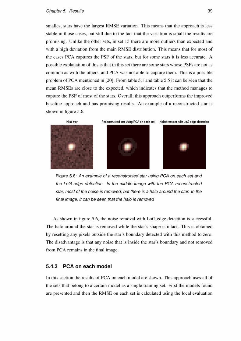
Chapter 5. Results 39
smallest stars have the largest RMSE variation. This means that the approach is less
stable in those cases, but still due to the fact that the variation is small the results are
promising. Unlike the other sets, in set 15 there are more outliers than expected and
with a high deviation from the main RMSE distribution. This means that for most of
the cases PCA captures the PSF of the stars, but for some stars it is less accurate. A
possible explanation of this is that in this set there are some stars whose PSFs are not as
common as with the others, and PCA was not able to capture them. This is a possible
problem of PCA mentioned in [20]. From table 5.1 and table 5.5 it can be seen that the
mean RMSEs are close to the expected, which indicates that the method manages to
capture the PSF of most of the stars. Overall, this approach outperforms the improved
baseline approach and has promising results. An example of a reconstructed star is
shown in figure 5.6.
Figure 5.6: An example of a reconstructed star using PCA on each set and
the LoG edge detection. In the middle image with the PCA reconstructed
star, most of the noise is removed, but there is a halo around the star. In the
final image, it can be seen that the halo is removed
As shown in figure 5.6, the noise removal with LoG edge detection is successful.
The halo around the star is removed while the star’s shape is intact. This is obtained
by resetting any pixels outside the star’s boundary detected with this method to zero.
The disadvantage is that any noise that is inside the star’s boundary and not removed
from PCA remains in the final image.
5.4.3 PCA on each model
In this section the results of PCA on each model are shown. This approach uses all of
the sets that belong to a certain model as a single training set. First the models found
are presented and then the RMSE on each set is calculated using the local evaluation

Chapter 5. Results 40
framework. After comparing the eigenvectors obtained from each set using PCA on
each set, 3 distinct patterns were found. Each set was then combined with the rest of
the sets that had the same eigenvector patterns. These new combined sets represent the
data for each of the three models. In table 5.4 the model in which each set belongs to
is provided. In figure 5.7 the three patterns used for categorizing the sets to the models
they belong to are illustrated.
Figure 5.7: The patterns of each model. The eigenvectors of the sets that
belong to model 1 have a riple effect. In model 2 there are linear ripples
whereas in model 3 the eigenvectors have a starburst effect.
The eigenvectors of the sets that belong to model 1 have a ripple effect around
their main structure, whereas in model 2 linear ripples are also introduced. In model
3 the main characteristic of the eigenvectors is the starburst effect and that there are
no ripples. Each of these models might represent different atmospheric or telescopic
effects, so this method can also be used for identifying different effects on star images.
The RMSE scores on each set using PCA on each model are provided in figure 5.8
and table 5.6.

Chapter 5. Results 41
Figure 5.8: Box-plot of the RMSE on each set using PCA on each model.
The RMSEs are close to the expected but there are more outliers, which
indicates that some PSFs are not accurately captured.
Set 1 Set 2 Set 3 Set 4 Set 5 Set 6 Set 7mRMSE 0.00188 0.00175 0.00168 0.00188 0.00188 0.00320 0.00123
Set 8 Set 9 Set 10 Set 11 Set 12 Set 13 Set 14mRMSE 0.00166 0.00188 0.00157 0.00152 0.00165 0.00165 0.00269
Set 15 Set 16 Set 17 Set 18 Set 19 Set 20 Set 21mRMSE 0.00115 0.00188 0.00165 0.00188 0.00165 0.00188 0.00165
Set 22 Set 23 Set 24 Set 25 Set 26mRMSE 0.00158 0.00152 0.00166 0.00166 0.00270
Table 5.6: The mean RMSE of the reconstructed stars using PCA on each
model. The mean RMSEs are close to the expected, which indicates that
the method has good results. The scores are slightly better than the ones
obtained with PCA on each set.
From table 5.5 and table 5.6 it can be seen that PCA on each model has slightly
better results in most of the sets. The difference is approximately 1%, which is not
substantial. Only set 15 gets a 5% improvement over the PCA on each set results. This
difference is not big enough to suggest that this method should be preferred. Moreover,
as mentioned in Chapter 4, this method will probably have sets that are overfitting due

Chapter 5. Results 42
to the way the components are selected. From figure 5.8 it is obvious that the RMSEs
are not as stable as in PCA on each set. There are more sets now where outliers appear
with a higher deviation from their main RMSE distribution than the expected one. The
stars on which this happens are not many but it is mainly affecting the sets of model
2 and model 3. Since more data are used as a training set, it is possible that some
stars with PSFs that are not that common were not taken into consideration by PCA,
resulting in not being reconstructed with high accuracy. The reason that this did not
happen in PCA on each set is that the data were smaller, so if a few of these uncommon
PSFs existed, because of the smaller size of data they were considered important and
taken into consideration. A recreation of a star is illustrated in figure 5.9, showing that
the approach manages to remove the noise from the initial star.
Figure 5.9: An example of a reconstructed star using PCA on each model
and the LoG edge detection. The PCA reconstructed star has some noise
and a halo around its boundary . In the final image, it can be seen that the
halo and the noise is removed
Compared to the reconstructed star using PCA on each set, the reconstructed star
using this method looks like it has more noise around the star’s boundary. This means
that there is probably more noise inside the star boundary as well. If this is the case
then the results using this method have lower RMSEs because the method is overfitting.
Even though it is not clear if this method is better or not, it will be tested using the
global evaluation framework for obtaining its true quality. It clearly has better results
than the improved baseline approach and its RMSEs are close to the expected, which
means that it is worth using.

Chapter 5. Results 43
5.4.4 PCA on all of the sets
The final method using PCA is the one that uses all of the data as training set. The
results of this method using the local evaluation framework are provided in figure 5.10
and in table 5.7.
Figure 5.10: Box-plot of the RMSE on each set using PCA on all of the
sets.The RMSEs are close to the expected but there are more outliers, which
indicates that some PSFs are not accurately captured.
Set 1 Set 2 Set 3 Set 4 Set 5 Set 6 Set 7mRMSE 0.00187 0.00174 0.00167 0.00187 0.00187 0.00319 0.00121
Set 8 Set 9 Set 10 Set 11 Set 12 Set 13 Set 14mRMSE 0.00166 0.00187 0.00155 0.00150 0.00165 0.00165 0.00268
Set 15 Set 16 Set 17 Set 18 Set 19 Set 20 Set 21mRMSE 0.00112 0.00187 0.00165 0.00187 0.00165 0.00187 0.00165
Set 22 Set 23 Set 24 Set 25 Set 26mRMSE 0.00156 0.00151 0.00166 0.00166 0.00269
Table 5.7: The mean RMSE of the reconstructed stars using PCA on all of
the sets. The mean RMSEs are close to the expected, which indicates that
the method has good results. The scores are slightly better than the ones
obtained with PCA on each set except set 7.

Chapter 5. Results 44
Comparing table 5.5 and table 5.6, the results of this method are slightly better than
PCA on each set, except set 7. The mean RMSE is approximately 1% better in all of
the sets except set 7 where it is 1% worse and set 15 that is 9% better. As was the case
with PCA on each model, the RMSE scores are less stable than the ones obtained with
PCA on each set for the same reasons. A recreation of a star is illustrated in figure
5.11.
Figure 5.11: An example of a reconstructed star using PCA on all of the sets
and the LoG edge detection. The PCA reconstructed star has some noise
and a halo around its boundary . In the final image, it can be seen that the
halo and the noise is removed
The final reconstructed star in figure 5.11 has the same shape as the other two meth-
ods using PCA. If the reconstructed star in the middle image of the figure is compared
with that of PCA on each model and PCA on each set, then it is clear that there is
more noise around the star. This means that there is probably more noise inside the
star’s boundary as well. As with the previous method, there is a chance that the RMSE
scores are lower due to overfitting, hence it is not clear if it is better than the other PCA
approaches.
5.5 ICA
This section provides the results concerning ICA. First the number of components
that is used on each set is provided. Then the results of different contrast functions are
presented. Finally, the results of ICA with the selected contrast function are illustrated.
5.5.1 Component Selection
In table 5.8 the components used on each set with each contrast function is shown. The
components were selected by hand, by visualizing them and selecting the ones that

Chapter 5. Results 45
have apparent structure as described in the previous chapter. The contrast functions
were tested on a subset of sets and then the selected contrast function was tested on
each set. Any sets for which a contrast function does not have a number of components
it means that it wasn’t tested on that set.

Chapter 5. Results 46
ICA on each set
Set Gauss Tanh Kurtosis
1 10 10 9
2 10 10 9
3 10 - -
4 10 - -
5 10 - -
6 15 - -
7 10 - -
8 12 - -
9 20 19 19
10 16 - -
11 12 - -
12 16 - -
13 14 - -
14 16 15 15
15 11 12 11
16 8 - -
17 16 - -
18 6 - -
19 15 - -
20 10 - -
21 13 - -
22 11 11 11
23 15 - -
24 11 - -
25 10 - -
26 13 12 13
Table 5.8: The number of components used with each ICA contrast function.
If no value is provided it means that the contrast function was not tested on
that set.

Chapter 5. Results 47
5.5.2 Contrast function selection
For selecting the final contrast function to be used, the RMSE scores obtained using the
local evaluation framework were used. The RMSE scores on each set that the functions
were tested are presented in a box-plot in figure 5.12 and the mean RMSE is provided
in table 5.9. These results are obtained using 10% of the stars of each set that they
were tested on, as mentioned in the local evaluation framework section in Chapter 4.
Figure 5.12: Box-plot of the RMSE on the sets ICA was tested using differ-
ent contrast functions. G with a number represents the Gaussian contrast
function on the set with that number. K is for the kurtosis contrast function
and T is for the tanh contrast function. The RMSEs have a smaller variance
with the Gaussian contrast function, except in set 22.
Set 1 Set 2 Set 9 Set 14 Set 15 Set 22 Set 26Gaussian 0.00193 0.00181 0.00205 0.00275 0.00126 0.00160 0.00279
Kurtosis 0.00213 0.00185 0.00207 0.00284 0.00127 0.00159 0.00279
Tanh 0.00204 0.00183 0.00207 0.00284 0.00126 0.00160 0.00280
Table 5.9: The mean RMSE on the sets ICA was tested with each contrast
function. The best scores are obtained using the Gaussian contrast function
except in set 22.
From figure 5.12 it can be seen that the RMSE scores have a smaller variance for

Chapter 5. Results 48
the Gaussian contrast function. Only in set 22 the deviation is a bit higher than the
scores obtained with the kurtosis contrast function. Moreover, the mean RMSE of the
Gaussian contrast function is smaller in all of the sets except set 22 as was the case
with the deviation of the RMSE scores. These two reasons led to choose the Gaussian
contrast function as the one used for analysing the data with ICA.
5.5.3 ICA on each set
The results of ICA with the Gaussian contrast function and using each set as a dif-
ferent training set are presented. The RMSE on each set is calculated using the local
evaluation framework using all of the stars. The RMSE on each set and its variation is
shown with a box-plot in figure 5.13 and the mean RMSE on each set is provided in
table 5.10.
Figure 5.13: Box-plot of the RMSE on each set using ICA on each set. The
RMSEs are close to the expected but there are many outliers in all of the
sets, which suggest that the method does not capture the PSF of all the
stars.

Chapter 5. Results 49
Set 1 Set 2 Set 3 Set 4 Set 5 Set 6 Set 7mRMSE 0.00194 0.00181 0.00183 0.00205 0.00205 0.00333 0.00121
Set 8 Set 9 Set 10 Set 11 Set 12 Set 13 Set 14mRMSE 0.00168 0.00204 0.00161 0.00164 0.00172 0.00176 0.00275
Set 15 Set 16 Set 17 Set 18 Set 19 Set 20 Set 21mRMSE 0.00126 0.00209 0.00172 0.00221 0.00173 0.00198 0.00179
Set 22 Set 23 Set 24 Set 25 Set 26mRMSE 0.00160 0.00154 0.00168 0.00173 0.00279
Table 5.10: The mean RMSE of the reconstructed stars using ICA on each
set. The mean RMSEs are close to the expected but are higher than those
obtained with PCA on each set.
The mean RMSE of this method on each set outperforms the improved baseline
approach and its RMSE scores are close to the expected, proving that this method is
better. But when compared to the PCA on each set results, it can be seen that PCA has
lower RMSEs. The mean RMSE on each set is 1 to 10% higher compared to that of
PCA. Moreover, from figure 5.13 it can be seen that the RMSE deviates often from the
main RMSE distribution of each set, hence the method is not as stable as PCA. Because
ICA makes the assumption that the sources are non-Gaussian, but one of the sources
is Gaussian (noise), it is possible that it does not manage to fully unmix the sources
resulting in worse results than PCA. An example of a reconstructed star is shown in
figure 5.14
Figure 5.14: An example of a reconstructed star using ICA on each set and
the LoG edge detection. In the middle image with the ICA reconstructed star,
most of the noise is removed, but there is a halo around the star. In the final
image, it can be seen that the halo is removed

Chapter 5. Results 50
As shown in figure 5.14, the initial star is denoised. The halo around the star is
removed while the star’s shape is maintained. By comparing the reconstructed star
with PCA on each set, it can be seen that the halo with ICA is slightly bigger, thus the
star has more noise in it.
5.6 Kernel PCA
In this section the results concerning kernel PCA are presented. First the number of
components that is used on each kernel PCA approach is provided. Then the results of
kernel PCA with the RBF kernel are shown and finally the results of kernel PCA with
the polynomial kernel.
5.6.1 Component Selection
The range of components tested and the final number of components selected for each
set in each kernel PCA approach are presented in table 5.11.
The lower boundary provided by the Scree test is the same for all the sets for both
of the kernels and is equal to 4. Of course Scree test is not that reliable since it can be
interpreted differently, but it was preferred to use the first elbow as the lower boundary
so that more components could be checked.
With the polynomial kernel, there was no apparent structure to the eigenvectors as
with PCA. Because of this, the upper boundary for using the noise variance technique
and defining the final upper boundary, was the dimensionality of the star patch (900).
On the other hand, with the RBF kernel, the first eigenvectors had structure. As with
PCA, the noise variance technique selected a lower number of components than the
one proposed by the eigenvector technique, except in set 32 that the same number of
components is proposed. As expected, the final number of components selected for
each set is the upper boundary of the range of number of components tested. This
is normal since when more components are used, more information is used for the
reconstruction of the stars, hence better results are obtained. As seen in table 5.12 the
number of components selected for the polynomial kernels is larger in most of the sets,
hence it is probable that the structure of the PSF is better captured than the RBF kernel.
The disadvantage of having more components is in the interpolation phase, since the
amount of time needed to predict the values increases.

Chapter 5. Results 51
RBF kernel Polynomial kernel
Set LB EUB FUB S LB EUB FUB S
1 4 47 22 22 4 - 35 35
2 4 47 22 22 4 - 39 39
3 4 47 21 21 4 - 42 42
4 4 52 30 30 4 - 36 36
5 4 50 25 25 4 - 35 35
6 4 26 17 17 4 - 18 18
7 4 37 15 15 4 - 83 83
8 4 43 21 21 4 - 61 61
9 4 54 32 32 4 - 40 40
10 4 54 25 25 4 - 68 68
11 4 60 28 28 4 - 72 72
12 4 61 33 33 4 - 63 63
13 4 44 22 22 4 - 62 62
14 4 34 34 34 4 - 28 28
15 4 32 15 15 4 - 120 120
16 4 46 24 24 4 - 37 37
17 4 50 25 25 4 - 63 63
18 4 46 21 21 4 - 35 35
19 4 50 25 25 4 - 64 64
20 4 46 21 21 4 - 35 35
21 4 50 26 26 4 - 64 64
22 4 44 21 21 4 - 65 65
23 4 50 22 22 4 - 68 68
24 4 49 30 30 4 - 59 59
25 4 34 17 17 4 - 59 59
26 4 30 23 23 4 - 26 26
Table 5.11: The range of components tested on each Kernel PCA method
and the selected number of components. LB is the lower boundary of the
range of number of components tested. EUB is the upper boundary given by
the visualisation of the eigenvectors. FUB is the final upper boundary given
by the noise variance technique. S is the selected number of components.

Chapter 5. Results 52
5.6.2 Kernel PCA on each set with a RBF kernel
Here, the results of kernel PCA with the RBF kernel are presented. The RMSE on
each set is calculated using the local evaluation framework using all of the stars. The
RMSE on each set is illustrated in figure 5.15 whereas table 5.13 has the mean RMSE
on each set.
Figure 5.15: Box-plot of the RMSE on each set using kernel PCA on each
set with the RBF kernel. The RMSEs are close to the expected and there
are not many outliers.
Set 1 Set 2 Set 3 Set 4 Set 5 Set 6 Set 7mRMSE 0.00191 0.00177 0.00170 0.00191 0.00190 0.00258 0.00159
Set 8 Set 9 Set 10 Set 11 Set 12 Set 13 Set 14mRMSE 0.00180 0.00190 0.00175 0.00173 0.00169 0.00169 0.00235
Set 15 Set 16 Set 17 Set 18 Set 19 Set 20 Set 21mRMSE 0.00145 0.00179 0.00169 0.00180 0.00169 0.00180 0.00169
Set 22 Set 23 Set 24 Set 25 Set 26mRMSE 0.00165 0.00162 0.00169 0.00169 0.00221
Table 5.12: The mean RMSE on each set using kernel PCA on each set with
the RBF kernel. The mean RMSEs are close to the noise mean RMSEs,
hence it is having good results. The scores are better than those in PCA on
sets with smaller stars and worse in those with larger stars.

Chapter 5. Results 53
The mean RMSE of each set provided in table 5.13 shows that this method out-
performs the improved baseline and it is close to the expected shown in table 5.1. Its
results when compared with the ones obtained from PCA on each set, are in some
cases better and in others worse. Specifically the big differences are in the sets with
big stars and the sets with the smaller stars. In sets with big stars, PCA has better re-
sults, whereas this method is better with sets with smaller stars. On the other hand, this
method looks like it is more stable than PCA. In figure 5.15, the RMSEs are deviating
less from the main RMSE distribution in each set and even in set 15 where all of the
other methods had a lot of outliers, in this case this is not happening. This characteris-
tic might suggest that the data in set 15 lie in a non linear subspace which kernel PCA
manages to capture. An example of a reconstructed star is shown in figure 5.16.
Figure 5.16: An example of a reconstructed star using kernel PCA on each
set with the RBF kernel and the LoG edge detection. The reconstructed star
with kernel PCA with the RBF kernel, removes most of the noise, but there is
a halo around the star. In the final image, the halo is removed with the LoG
edge detection
Kernel PCA with the RBF kernel manages to remove most of the noise except a
halo around the star. That is removed using the LoG edge detection while the star’s
shape is maintained. Compared to the PCA reconstructed star, the halo is smaller which
indicates that this method manages to remove more noise, hence is more effective.
5.6.3 Kernel PCA on each set with a Polynomial kernel
The results of kernel PCA with the polynomial kernel are provided in this section. The
RMSEs on each set are obtained using the local evaluation framework using all of the
stars. The RMSEs on each set are illustrated in figure 5.17 whereas table 5.14 has the
mean RMSE on each set.

Chapter 5. Results 54
Figure 5.17: Box-plot of the RMSE on each set using kernel PCA on each set
with the polynomial kernel. The RMSEs are close to the expected and the
outliers are fewer than the other methods used. Since fewer outliers exist,
this means that the method captures the PSF of more stars.
Set 1 Set 2 Set 3 Set 4 Set 5 Set 6 Set 7mRMSE 0.00190 0.00175 0.00168 0.00190 0.00190 0.00256 0.00158
Set 8 Set 9 Set 10 Set 11 Set 12 Set 13 Set 14mRMSE 0.00179 0.00189 0.00174 0.00171 0.00168 0.00168 0.00220
Set 15 Set 16 Set 17 Set 18 Set 19 Set 20 Set 21mRMSE 0.00144 0.00178 0.00168 0.00179 0.00168 0.00179 0.00168
Set 22 Set 23 Set 24 Set 25 Set 26mRMSE 0.00163 0.00160 0.00168 0.00168 0.00220
Table 5.13: The mean RMSE on each set using kernel PCA on each set with
the polynomial kernel. The mean RMSEs are close to the expected, which
indicates that the method is able to capture the PSF of the stars with good
results. These results are better than the ones obtained with the RBF kernel
As was the case with the other kernel, this method outperforms the improved base-
line approach as well. The results between the two kernels are quite similar. The
polynomial has slightly better results since its mean RMSE errors are 0.5 to 1% better
than those obtained with the RBF kernel. The main difference can be seen by com-

Chapter 5. Results 55
paring figure 5.15 and figure 5.17 where it can be seen that the RMSE variance in set
14 is reduced. Since the results are quite similar to the ones with the RBF kernel, the
comparison with PCA on each set is the same. An example of a reconstructed star is
shown in figure 5.18.
Figure 5.18: An example of a reconstructed star using kernel PCA on each
set with the RBF kernel and the LoG edge detection. The reconstructed star
with kernel PCA with the RBF kernel, removes almost all of the noise and
any remaining noise is reduced with the LoG edge detection
As shown in figure 5.18 this method manages to remove the noise from the initial
image. Kernel PCA with the polynomial kernel is the only method that manages to
remove the halo effect. The reconstructed image using looks like no noise is left.
In reality there is still some noise left but its value is almost zero. If the LoG edge
detection was not used, then this method would have the best results compared to the
rest of the methods. This method also captures an extra pixel at the bottom of the star
that the rest of the methods did not capture. It is not possible to know if this actually
belongs to the true star but it will be clear when all of these methods are used with the
global evaluation framework in future.
5.7 Comparison of the methods
The task of finding the true PSF of each star needs a method that is stable and is as
accurate as possible. The baseline approach and the improved baseline approach have
been proven unreliable. They are too sensitive to noise and the resulted stars have
higher pixel intensities than the original images and different shapes and sizes. For
these reasons, these methods are not worth using.
The dimensionality reduction techniques combined with the LoG edge detection

Chapter 5. Results 56
method for removing the noise have promising results and outperform the baseline
approaches. From their results it is not possible to conclude which method is better.
The only method that is less stable is ICA which had slightly worse results than the
other methods. The disadvantage of ICA, is that it has more stars whose RMSEs
deviate from the main RMSE distribution of their sets. These deviations suggest that
the method is not capturing the PSF of all the stars in the set. If it was, then it would
be expected that the box-plot in figure 5.14 would have less outliers. The reason for
expecting something like this is that if a method manages to remove the noise from a
star, then the RMSE of the residual of the reconstructed star and the initial noisy star
will account only for the noise of the initial image. The noise levels should be around
the same in each set, hence the RMSEs would have similar values. Moreover the mean
RMSEs of ICA are higher than the mean RMSEs obtained with PCA, but this might
not be a disadvantage, since lower RMSEs might mean that the method is overfitting.
Even though the mean RMSE of PCA on each set cannot indicate if the method
is better than ICA, in each set its RMSEs have less outliers than ICA, which suggests
that it has more stable results. Only in set 15 it is not able to capture the PSF of all
stars, thus the RMSEs of those stars deviate from the rest. Kernel PCA looks like it
has more stable results than the rest of the methods, since its RMSEs in each set have
less outliers and their deviation from the main RMSE distribution in each set is small.
Its results though, in some cases have larger mean RMSEs than PCA and in others
smaller mean RMSEs. It was expected that kernel PCA would have better results
than PCA since it is able to capture information that lies in non-linear subspaces as
well, but as noted smaller mean RMSEs using the local evaluation framework might
be caused from overfitting. If indeed PCA is better, a possible reason for having this
is that the reconstruction performed from the lower dimensions is naive and probably
information is lost. Since there is no clear way of defining if a method is overfitting
using these results, none of the dimensionality reduction techniques should be rejected
before actually using them with the global evaluation framework. This will provide
their true quality measure so that better conclusions can be made on each method.
Chapter 6
Conclusion
In this dissertation, the problem of finding the PSF of a star and recreating the star
with that PSF with high accuracy is addressed. Initially two baseline approaches are
used, which are based on the use of quadrupole moments. As expected they were
found inappropriate for this problem because they were affected by noise resulting to
inaccurate star reconstructions. Two evaluation frameworks were proposed for eval-
uating different dimensionality reduction techniques and different techniques that can
be used to further remove any noise that was not effectively removed at the previous
steps. One of the frameworks uses the evaluation provided by the GREAT10 star chal-
lenge website, but was not used because the values at the non-star positions are still
being interpolated. The second framework allows to optimize the techniques locally
by comparing the reconstructed stars with the initial noisy stars.
The three dimensionality reduction techniques used are PCA, ICA and kernel PCA
and they were combined with the LoG edge detection. It has been shown that LoG
edge detection can remove any noise that is outside the boundary of the reconstructed
star but cannot be used for removing noise inside the stars boundary. This is the first
time ICA and kernel PCA are used for capturing the PSF and their results are close to
the expected RMSEs suggesting that they are suitable for this task. PCA was also used
to provide data to the students who were working with the interpolation part of the
GREAT10 star challenge. This included an exploratory data analysis with PCA to find
possible models that were used for creating the stars and which sets belonged to each
model. The results of the three dimensionality reduction techniques with LoG edge
detection are promising and outperformed the baseline approaches. It is not possible
to say with certainty which method is better using the results of the local evaluation
framework, but kernel PCA and PCA seem to be better than ICA, mainly because they
57

Chapter 6. Conclusion 58
have less outliers in their RMSEs distributions. Specifically kernel PCA has fewer
RMSEs deviating from the main RMSE distribution in each set and because of its non
linearity it can capture PSFs that the other techniques cannot. Once all of the values
are predicted on the asked non-star positions, the true quality of each method will be
obtained using the global evaluation framework.
6.1 Future work
The first thing that is worth trying is the global evaluation framework using the opti-
mised methods obtained from this dissertation. This will be done as soon as all the
values at the non-star positions are interpolated. The values are already being interpo-
lated and they should be available soon. Also the way that the data were reconstructed
from their lower dimensions with kernel PCA can be improved and will probably lead
to better results. Since kernel PCA seems to be more stable than the other methods, if
it gets better RMSE scores using a different reconstruction method, it will become a
reliable technique for this task. ICA can also be improved by using a genetic algorithm
for selecting the optimal components. Finally since LoG edge detection cannot be used
to remove the noise inside the boundary of a star, other denoising techniques can be
tested for removing the remaining noise of the reconstructed stars.

Bibliography
[1] Herv Abdi and Lynne J. Williams. Principal component analysis. Wiley Interdis-ciplinary Reviews: Computational Statistics, pages n/a–n/a, June 2010.
[2] A. Aizerman, E.M. Braverman, and LI Rozoner. Theoretical foundations of thepotential function method in pattern recognition learning. Automation and remotecontrol, 25:821–837, 1964.
[3] B.E. Boser, I.M. Guyon, and V.N. Vapnik. A training algorithm for optimal mar-gin classifiers. In Proceedings of the fifth annual workshop on Computationallearning theory, pages 144–152. ACM, 1992.
[4] S. Bridle, S. T Balan, M. Bethge, M. Gentile, S. Harmeling, C. Heymans,M. Hirsch, R. Hosseini, M. Jarvis, D. Kirk, et al. Results of the GREAT08 chal-lenge: an image analysis competition for cosmological lensing. Monthly Noticesof the Royal Astronomical Society, 405(3):20442061, 2010.
[5] S. Bridle, J. Shawe-Taylor, A. Amara, D. Applegate, S.T. Balan, J. Berge,G. Bernstein, H. Dahle, T. Erben, M. Gill, et al. Handbook for the great08 chal-lenge: An image analysis competition for cosmological lensing. The Annals ofApplied Statistics, 3(1):6–37, 2009.
[6] J.S. Chen and G. Medioni. Detection, localization, and estimation of edges. Pat-tern Analysis and Machine Intelligence, IEEE Transactions on, 11(2):191–198,1989.
[7] J.J. Clark. Authenticating edges produced by zero-crossing algorithms. PatternAnalysis and Machine Intelligence, IEEE Transactions on, 11(1):43–57, 1989.
[8] P. Comon. Independent component analysis, a new concept? Signal processing,36(3):287–314, 1994.
[9] Gene Howard Golub and Charles F. Van Loan. Matrix computations. JHU Press,October 1996.
[10] R.C. Gonzalez and R.E. Woods. Digital image processing. 1992. Reading, Mass.:Addison-Wesley, 16(716):8.
[11] S.R. Gunn. On the discrete representation of the laplacian of gaussian. PatternRecognition, 32(8):1463–1472, 1999.
59

Bibliography 60
[12] D. Huterer. Weak lensing, dark matter and dark energy. General Relativity andGravitation, page 119, 2010.
[13] A. Hyvarinen. Fast and robust fixed-point algorithms for independent componentanalysis. Neural Networks, IEEE Transactions on, 10(3):626634, 1999.
[14] A. Hyvarinen, PO Hoyer, and E. Oja. Image denoising by sparse code shrinkage,2001.
[15] A. Hyvrinen and E. Oja. Independent component analysis: algorithms and appli-cations. Neural Networks, 13(4-5):411–430, June 2000.
[16] R. Jain, R. Kasturi, and B.G. Schunck. Machine vision, volume 5. McGraw-HillNew York, 1995.
[17] M. Jarvis and B. Jain. Principal component analysis of PSF variation in weaklensing surveys. Arxiv preprint astro-ph/0412234, 2004.
[18] M. J. Jee, J. P. Blakeslee, M. Sirianni, A. R. Martel, R. L. White, and H. C. Ford.Principal component analysis of the time-and position-dependent Point-Spreadfunction of the advanced camera for surveys. Publications of the AstronomicalSociety of the Pacific, 119(862):14031419, 2007.
[19] I. T. Jolliffe. Principal component analysis. Springer, 2002.
[20] Thomas Kitching, Adam Amara, Mandeep Gill, Stefan Harmeling, CatherineHeymans, Richard Massey, Barnaby Rowe, Tim Schrabback, Lisa Voigt, Sreeku-mar Balan, Gary Bernstein, Matthias Bethge, Sarah Bridle, Frederic Courbin,Marc Gentile, Alan Heavens, Michael Hirsch, Reshad Hosseini, Alina Kiessling,Donnacha Kirk, Konrad Kuijken, Rachel Mandelbaum, Baback Moghaddam,Guldariya Nurbaeva, Stephane Paulin-Henriksson, Anais Rassat, Jason Rhodes,Bernhard Schlkopf, John Shawe-Taylor, Marina Shmakova, Andy Taylor, Ma-lin Velander, Ludovic van Waerbeke, Dugan Witherick, and David Wittman.Gravitational lensing accuracy testing 2010 (GREAT10) challenge handbook.1009.0779, September 2010.
[21] J.T.Y. Kwok and I.W.H. Tsang. The pre-image problem in kernel methods. Neu-ral Networks, IEEE Transactions on, 15(6):1517–1525, 2004.
[22] S. Makeig, A.J. Bell, T.P. Jung, T.J. Sejnowski, et al. Independent componentanalysis of electroencephalographic data. In Proceedings of the 1995 conference,volume 8, page 145. Kaufmann, 1996.
[23] D. Marr and E. Hildreth. Theory of edge detection. Proceedings of the RoyalSociety of London. Series B. Biological Sciences, 207(1167):187, 1980.
[24] Y. Mellier. Probing the universe with weak lensing. astro-ph/9812172, December1998. Ann.Rev.Astron.Astrophys. 37 (1999) 127-189.

Bibliography 61
[25] S. Mika, B. Scholkopf, A. J Smola, K. R Muller, M. Scholz, and G. Ratsch.Kernel PCA and de-noising in feature spaces. Advances in neural informationprocessing systems, 11(1):536542, 1999.
[26] R. Nakajima, GM Bernstein, R. Fadely, CR Keeton, and T. Schrabback. Im-proved constraints on the gravitational lens q0957+ 561. i. weak lensing. TheAstrophysical Journal, 697:1793, 2009.
[27] J.M.S. Prewitt. Object enhancement and extraction, volume 75. Academic Press,New York, 1970.
[28] J. Sarela and H. Valpola. Denoising source separation. Journal of Machine Learn-ing Research, 6:233–272, 2005.
[29] Bernhard Schlkopf, Alexander Smola, and Klaus-Robert Mller. Kernel principalcomponent analysis. 1999.
[30] T. Schrabback, J. Hartlap, B. Joachimi, M. Kilbinger, P. Simon, K. Benabed,M. Bradac, T. Eifler, T. Erben, C.D. Fassnacht, et al. Evidence for the acceleratedexpansion of the universe from weak lensing tomography with cosmos. Arxivpreprint arXiv:0911.0053, 2009.
[31] AR Teixeira, AM Tome, K. Stadlthanner, and EW Lang. Kpca denoising and thepre-image problem revisited. Digital Signal Processing, 18(4):568–580, 2008.
[32] M. Titsias and N. Lawrence. Bayesian gaussian process latent variable model.2010.
[33] LJP Van der Maaten, EO Postma, and HJ Van den Herik. Dimensionality reduc-tion: A comparative review. Preprint, 2007.
[34] P.G. Van Dokkum. Cosmic-ray rejection by laplacian edge detection. Arxivpreprint astro-ph/0108003, 2001.
[35] J. Wang and C. I Chang. Independent component analysis-based dimensional-ity reduction with applications in hyperspectral image analysis. Geoscience andRemote Sensing, IEEE Transactions on, 44(6):15861600, 2006.