Embed Size (px)
Citation preview

Dimensionality reduction in big data sets
Gudmund Horn Hermansen
Department of Mathematics at University of Oslo
26 September 2014
1/46

What are the big data phenomena?
• Typically characterised by high dimensionality and/or largesample sizes.
• Granularity and heterogeneities.
• Collection of massive datasets for both ‘classical’ statistical testingand for exploratory science.
• A meeting point of computer science and statistics.
• Sensor network, monitoring, physics, astronomy, genomics, human(online) activity, images, voice translation, documents, ...
2/46
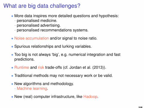
What are big data challenges?
• More data inspires more detailed questions and hypothesis:- personalised medicine.- personalised advertising.- personalised recommendations systems.
• Noise accumulation and/or signal to noise ratio.
• Spurious relationships and lurking variables.
• Too big is not always ‘big’, e.g. numerical integration and fastpredictions.
• Runtime and risk trade-offs (cf. Jordan et al. (2013)).
• Traditional methods may not necessary work or be valid.
• New algorithms and methodology.- Machine learning.
• New (real) computer infrastructure, like Hadoop.
3/46

Why dimensionality reduction?
• Making a massive datasets somewhat less massive.
• Data compression.
• Visualisation.
• More accurate and relevant representations of data.
• Runtime and memory, storage and bandwidth bottlenecks.
• Validity and accuracy of algorithms.
4/46

Outline
Machine learning
Principal component analysis (PCA)
Unsupervised feature learning
Regression and LASSO
Sufficiency
Focused dimensionality reduction
5/46
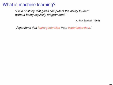
What is machine learning?“Field of study that gives computers the ability to learnwithout being explicitly programmed.”
Arthur Samuel (1969)
“Algorithms that learn/generalise from experience/data.”
6/46
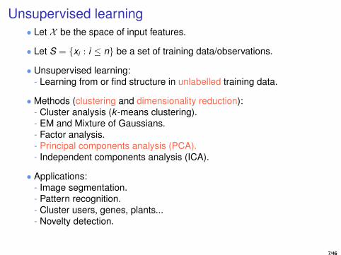
Unsupervised learning• Let X be the space of input features.
• Let S = {xi : i ≤ n} be a set of training data/observations.
• Unsupervised learning:- Learning from or find structure in unlabelled training data.
• Methods (clustering and dimensionality reduction):- Cluster analysis (k -means clustering).- EM and Mixture of Gaussians.- Factor analysis.- Principal components analysis (PCA).- Independent components analysis (ICA).
• Applications:- Image segmentation.- Pattern recognition.- Cluster users, genes, plants...- Novelty detection.
7/46
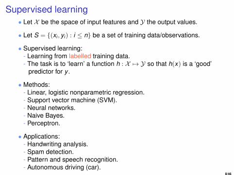
Supervised learning• Let X be the space of input features and Y the output values.
• Let S = {(xi , yi) : i ≤ n} be a set of training data/observations.
• Supervised learning:- Learning from labelled training data.- The task is to ‘learn’ a function h : X 7→ Y so that h(x) is a ‘good’
predictor for y .
• Methods:- Linear, logistic nonparametric regression.- Support vector machine (SVM).- Neural networks.- Naive Bayes.- Perceptron.
• Applications:- Handwriting analysis.- Spam detection.- Pattern and speech recognition.- Autonomous driving (car).
8/46

Supervised learning• Let X be the space of input features and Y the output values.
• Let S = {(xi , yi) : i ≤ n} be a set of training data/observations.
• Supervised learning:- Learning from labelled training data.- The task is to ‘learn’ a function h : X 7→ Y so that h(x) is a ‘good’
predictor for y .
•What about focused supervised learning?
• Make good estimators for a general focus parameter µ.- Predictions and forecasts.- Confidence bounds and quantiles.- Threshold probabilities.
9/46

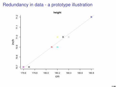
Redundancy in data - a prototype illustration
179.6 179.8 180.0 180.2 180.4 180.6 180.8
70.7
70.8
70.9
71.0
71.1
71.2
height
cm
inch
10/46
Redundancy in data - a prototype illustration
179.6 179.8 180.0 180.2 180.4 180.6 180.8
70.7
70.8
70.9
71.0
71.1
71.2
height
cm
inch
11/46
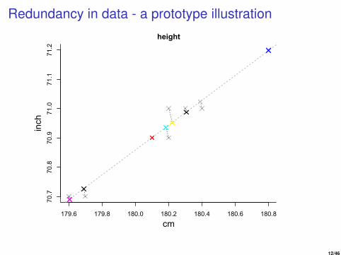
Redundancy in data - a prototype illustration
179.6 179.8 180.0 180.2 180.4 180.6 180.8
70.7
70.8
70.9
71.0
71.1
71.2
height
cm
inch
12/46

Redundancy in data - a prototype illustration
179.6 179.8 180.0 180.2 180.4 180.6 180.8
height
13/46

Principal component analysis (PCA)
• The most common and by far the most used algorithm fordimensionality reduction.
• Finds the ‘best’ lower-dimensional subspace with respect tominimising squared projection error.
• Let x1, . . . , xn, where xi ∈ Rm, then for a given k ≤ m PCA finds the‘best’ k -dimensional subspace u1, . . . ,uk , with ul ∈ Rk .
• Motivates an approximation of x1, . . . , xn in the linear subspacespanned by u1, . . . ,uk , i.e.
(x1, . . . , xn), where xi =
k∑l=1
αi,juj ≈ xi , for i ≤ n,
for certain weights αi,j .
• Unsupervised.
• Singular value decomposition (SVD).
14/46

PCA illustration
-4 -2 0 2 4 6 8
-10
12
34
56data
x1
x 2
data
15/46

PCA illustration
-4 -2 0 2 4 6 8
-10
12
34
56data
x1
x 2
dataPC axes
16/46
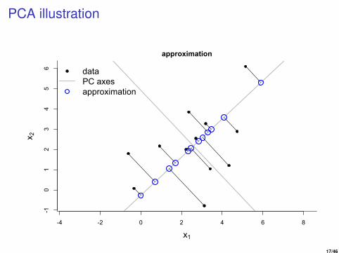
PCA illustration
-4 -2 0 2 4 6 8
-10
12
34
56
approximation
x1
x 2
dataPC axesapproximation
17/46
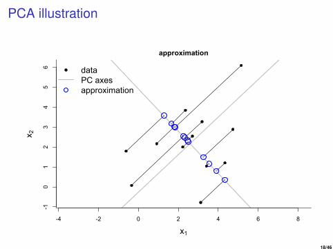
PCA illustration
-4 -2 0 2 4 6 8
-10
12
34
56
approximation
x1
x 2
dataPC axesapproximation
18/46

PCA is not linear regression
-4 -2 0 2 4 6 8
-10
12
34
56
approximation
x1
x 2
dataLM fitPC axesapproximation
19/46

Text classification illustration• Dictionary with e.g. 50000 words:
aapa, aardvark, aardwolf, aargh, abaca, aback, abacus, ...
• Document i is represented as a vector xi ∈ R50000, for i = 1, . . . ,n.
• The elements of
xi,j = 1 if word j in dictionary is in document i ,
and 0 otherwise.
• Sparse vectors in a very high-dimensional space.
• Documents are seen as similar if the angle between them is small,i.e.
∆(xi , xj) = cos(θ) =x t
i xj
‖xi‖ ‖xj‖,
where θ is the angle between xi and xj .
20/46

Text classification illustration• Consider documents about transportation, will typically include
words like bus, car, vehicle, bike, ...
• Note that the nominator of ∆(xi , xj) is
x ti xj =
k∑l=1
I(documents i and j contain word l),
which is 0 if the documents have no common words.
0.0 0.2 0.4 0.6 0.8 1.0
0.0
0.2
0.4
0.6
0.8
1.0 xj
xi
car
vehicle
21/46

Text classification illustration• Consider documents about transportation, will typically include
words like bus, car, vehicle, bike, ...
• Note that the nominator of ∆(xi , xj) is
x ti xj =
k∑l=1
I(documents i and j contain word l),
which is 0 if the documents have no common words.
0.0 0.2 0.4 0.6 0.8 1.0
0.0
0.2
0.4
0.6
0.8
1.0 xj
xi
ul
car
vehicle
22/46
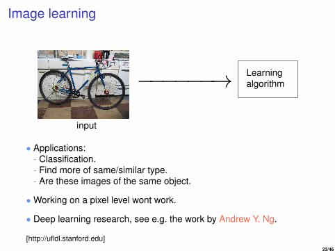
Image learning
input
−−−−−−→ Learningalgorithm
• Applications:- Classification.- Find more of same/similar type.- Are these images of the same object.
•Working on a pixel level wont work.
• Deep learning research, see e.g. the work by Andrew Y. Ng.
[http://ufldl.stanford.edu]23/46
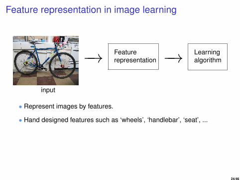
Feature representation in image learning
input
−→ Featurerepresentation −→ Learning
algorithm
• Represent images by features.
• Hand designed features such as ‘wheels’, ‘handlebar’, ‘seat’, ...
24/46

Feature representation
Input −−→ Featurerepresentation −−→ Learning
algorithm
• The feature representation is how the algorithm sees the world.- Reduce the dimensionality.- More relevant data representation.- Data compression.- Reduce noise.- Standard methodology.
• Handmade, which is hard, time consuming and require expertknowledge.
• Separate communities (vision, audio, text, ...) has uniquelydesigned features.
• Is there a better way?
25/46

Biological inspiration
• The auditory cortex ‘learns’ how to see.
• The ‘one learning algorithm’ hypothesis.
26/46
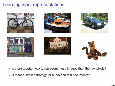
Learning input representations
• Is there a better way to represent these images than the raw pixels?
• Is there a similar strategy for audio and text documents?
27/46

Feature learning• Is there a better representation for a 14x14 image patch x from than
by 196 (raw pixel insensitive) numbers in a vector.
→
18912454
7832...
• How to make a feature representation without any hand design?
28/46

Classification illustrationbikes motorcycles
bike?
random
29/46

Feature learning by sparse coding• Sparse coding was developed in Olshausen & Field (1997) to
explain visual processing in the brain.
• Image input x1, . . . , xn, where xi ∈ Rm×m.
• The idea is to ‘learn’ a set of basis functions φ1, . . . , φk , whereφj ∈ Rm×m, such that each input
x ≈k∑
j=1
ajφj ,
with the restriction that (a1, . . . ,ad ) is mostly sparse.
30/46

Sparse coding illustration
→
• Example patch:
≈ 0.6× + 0.4× + 0.8×
31/46
Unsupervised feature learning• The algorithm ‘invents’ edge detection.
• Hopefully a better representation.
• Is similar to how we believe the brain process images in visualcortex (area V1) in the brain.
•Works for audio, text and other types of complex data.
• Is better than many of the old standards with hand designedfeatures.
[http://ufldl.stanford.edu]32/46

Outline
Machine learning
Principal component analysis (PCA)
Unsupervised feature learning
Regression and LASSO
Sufficiency
Focused dimensionality reduction
33/46
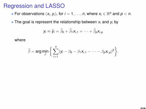
Regression and LASSO• For observations (xi , yi), for i = 1, . . . ,n, where xi ∈ Rp and p < n.
• The goal is represent the relationship between xi and yi by
yi ≈ yi = β0 + β1xi,1 + · · ·+ βpxi,p
where
β = arg minβ
{ n∑i=1
(yi − β0 − β1xi,1 − · · · − βpxi,p)2}.
34/46

Regression and LASSO• For observations (xi , yi), for i = 1, . . . ,n, where xi ∈ Rp and p < n.
• The goal is represent the relationship between xi and yi by
yi ≈ yi = β0 + β1xi,1 + · · ·+ βpxi,p
by adding a penalty to the estimation
β = arg minβ
{ n∑i=1
(yi − β0 − β1xi,1 − · · · − βpxi,p)2 + λ
p∑j=1
|βj |}
we obtain the LASSO.
• Some β coefficients may be set to zero.
• Feature selection or dimensionality reduction.
35/46

Regression and LASSO• If n < p standard methodology does not work.
• Use PCA or another type of dimensionality reduction as anintermediate step.
• Forward selection: Start with an empty set of features.- Find the optimal feature xi by e.g. p-value or cross-validation.- Include this in your feature set.- Include features until the stopping rule is satisfied.
• Testing all plausible subsets is NP-hard.
• Preselection: Make order list of features- By e.g. pairwise correlations cor(y , xj) for each j = 1, . . . ,p.- Include features until the stopping rule is satisfied.
• Focused preselection and dimensionality reduction.
36/46
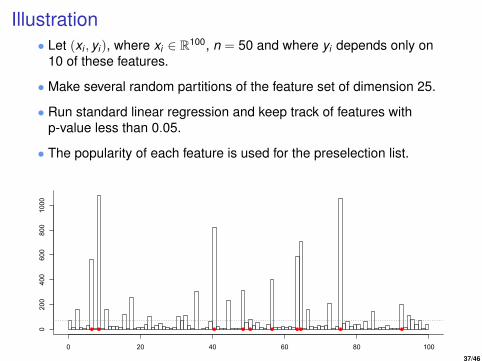
Illustration• Let (xi , yi), where xi ∈ R100, n = 50 and where yi depends only on
10 of these features.
• Make several random partitions of the feature set of dimension 25.
• Run standard linear regression and keep track of features withp-value less than 0.05.
• The popularity of each feature is used for the preselection list.
0 20 40 60 80 100
0200
400
600
800
1000
37/46

Illustration• Let (xi , yi), where xi ∈ R100, n = 50 and where yi depends only on
10 of these features.
• Make several random partitions of the feature set of dimension 25.
• Run standard linear regression and keep track of features withp-value less than 0.05.
• The popularity of each feature is used for the preselection list.
• The stopping rule is ‘significant on a 0.05 level’ and less than 25features.
• This ‘finds’ 10 correct features.
• ‘Standard’ preselection select only 6 features, where all are correct.
• Forward selection ends up with 25, including the 10 correct features.
38/46

Large samples (and high-dimensional feature spaces)• Long time series:
- Econometrics.- Stock market trading.- Auctions.
• Monitoring:- Network traffic.- Public security.- Production at a factory.- Air pollution.
• Predicting time to failure, predict crossing of threshold value,classifying behaviour, ...
• Fast and reliable predictions.
39/46

Sufficiency• As a prototype example suppose x1, . . . , xn i.i.d. with xi ∼ N(µ, σ2),
then
s1 =1n
n∑i=1
xi and s2 =1n
n∑i=1
x2i
are sufficient statistics for µ and σ2.
• Dimensionality reduction without (relative) loss of information.
• Exponential class of models:
f (y , θ) = g(y) exp{θtT (y)− c(θ)}
for a suitable T (y) = (T1(y), . . . ,Tp(y))t.
• In exponential families the dimensionality of the sufficient statisticdoes not increase as the sample size n increases.
• Fast updates for on-line data streams.
40/46

Sufficient dimension reduction• In regression the main interest are properties of y |x .
• Let R(x) represent a reduction of x .
• It is said to be a sufficient reduction if the distribution of y |R(x) isthe same as y | x , see e.g. Adragni & Cook (2009).
• No information is lost if the model is correctly specified.
• As an illustration, consider the model
y = α+ βtx + εi ,
where x is conditionally independent of ε and the distribution of y | xis the same as y |βtx .
• Focused sufficient dimensionality reduction, i.e. a reduction thatresults in no loss with respect to a chosen focus parameter.
41/46

Why focused dimensionality reduction?
• Interested in the bright and clear objects.
• But also the background signal.
• Dimensionality reduction should take this into account.
[Big Dipper: The Universe]42/46

Why focused dimensionality reduction?
• Runtime.
• More accurate predictions with larger samples of relevant data.
[www.luftkvalitet.info]43/46
Why focused dimensionality reduction?
• Runtime.
• Advertising, reading suggestions and recommendations.
[www.aftenposten.no]44/46

Concluding Remarks• Focused inference and methodology.
• Scaling up, more data and more features is (usually) moreimportant than smart algorithms Coates et al. (2011).
• Sometimes high dimensionally is ‘good’ as in some kernel methods.
• Vapnik–Chervonenkis (VC) dimension.
• Related methodology:- Hierarchical models.- Bayesian nonparametrics.- Clustering.- Support vector machine (SVD).- Classification.- Partial least squares regression (PLS).- Online learning.- Random forest.- Independent component analysis (ICA).- Subsampling and bag of little bootstraps.
45/46
Bibliography
ADRAGNI, K. P. & COOK, R. D. (2009). Sufficient dimensionreduction and prediction in regression. Philosophical Transactionsof the Royal Society A: Mathematical, Physical and EngineeringSciences 367, 4385–4405.
COATES, A., NG, A. Y. & LEE, H. (2011). An analysis of single-layernetworks in unsupervised feature learning. In InternationalConference on Artificial Intelligence and Statistics.
JORDAN, M. I. et al. (2013). On statistics, computation andscalability. Bernoulli 19, 1378–1390.
OLSHAUSEN, B. A. & FIELD, D. J. (1997). Sparse coding with anovercomplete basis set: A strategy employed by v1? Visionresearch 37, 3311–3325.
46/46