Page 1

DIGITAL IMAGE FILTERING

By Fred Weinhaus

Traditional (Static Weight) Convolution One method of filtering an image is to apply a convolution operation to the image to achieve: blurring, sharpening, edge extraction or noise removal. The action of a convolution is simply to multiply the pixels in the neighborhood of each pixel in the image by a set of static weights and then replace the pixel by the sum of the product. In order to prevent the overall brightness of the image from changing, the weights are either designed to sum to unity or the convolution is followed by a normalization operation, which divides the result by the sum of the weights. In simple terms, perform a weighted average in the neighborhood of each pixel and replace the pixel’s value by the average. Thus, the filter is generated by providing a set of weights to apply to the corresponding pixels in a given size neighborhood. The set of weights make up what is called the convolution kernel and is typically represented in a table or matrix-like form, where the position in the table or matrix corresponds to the appropriate pixel in the neighborhood. Such a convolution kernel (or filter) is typically a square of odd dimensions so that, when applied, the resulting image does not shift a half pixel relative to the original image. The general form for a 3x3 convolution kernel looks as follows:

€

w1 w2 w3w4 w5 w6w7 w8 w8

⎡

⎣

⎢ ⎢ ⎢

⎤

⎦

⎥ ⎥ ⎥

Page 2

or if the weights are not designed to sum to unity, then as

€

1sumw

w1 w2 w3w4 w5 w6w7 w8 w8

⎡

⎣

⎢ ⎢ ⎢

⎤

⎦

⎥ ⎥ ⎥

where sumw=(w1+w2+w3+w4+w5+w6+w7+w8+w9). In systems such as ImageMagick, normalization is done automatically as part of the convolution. Thus, the multiply by 1/sumw is not needed. But note that this factor must be taken into account if this filter is mixed with other filters to generate a more complex convolution, as will be done later. In ImageMagick, convolution kernels (filters) are represented as 1D comma separate lists and are created from the 2D kernel by appending each row to the end of the previous one. Thus in ImageMagick, the convolution kernel would be expressed as

Convert infile –convolve "w1,w2,w3,w4,w5,w6,w7,w8,w9" outfile Uniform Weight Convolutions The simplest convolution kernel or filter is of size 3x3 with equal weights and is represented as follows:

€

1/9 1/9 1/91/9 1/9 1/91/9 1/9 1/9

⎡

⎣

⎢ ⎢ ⎢

⎤

⎦

⎥ ⎥ ⎥

=

€

19

€

1 1 11 1 11 1 1

⎡

⎣

⎢ ⎢ ⎢

⎤

⎦

⎥ ⎥ ⎥

= low pass filter.

This filter produces a simple average (or arithmetic mean) of the 9 nearest neighbors of each pixel in the image. It is one of a class of what are known as low pass filters. They pass low frequencies in the image or equivalently pass long wavelengths in the image, i.e. slow variations in image intensity. Conversely, they remove short wavelengths in the image, which correspond to abrupt changes in image

Page 3

intensity, i.e. edges. Thus we get blurring. Also, because it is replacing each pixel with an average of the pixels in its local neighborhood, one can understand why it tends to blur the image. Blurring is typical of low pass filters. The opposite of a low pass filter is a high pass filter. It passes only short wavelengths, i.e. where there are abrupt changes in intensity and removes long wavelengths, i.e. where the image intensity is varying slowly. Thus when applied to an image, it shows only the edges in the image. High pass filtering of an image can be achieved by the application of a low pass filter to the image and subsequently subtraction of the low pass filtered result from the image. In abbreviated terms, this is H = I – L, where H = high pass filtered image, I = original image and L = low pass filtered image. We can express this in terms of the filters (convolution kernels) by recognizing that this equation is equivalent to the following:

h

€

⊗I = i

€

⊗I - l

€

⊗I where h, i and l are the high pass, identity and low pass filter (convolution kernels), respectively and

€

⊗ means convolution (i.e. multiply each neighborhood pixel by it corresponding weight and sum up the products). The identity filter is that convolution kernel which when applied to the image leaves the image unchanged. Therefore,

i =

€

0 0 00 1 00 0 0

⎡

⎣

⎢ ⎢ ⎢

⎤

⎦

⎥ ⎥ ⎥

= identity kernel.

Page 4

Thus if we combine the identity and low pass filter kernels above as specified, we get

h =

€

0 0 00 1 00 0 0

⎡

⎣

⎢ ⎢ ⎢

⎤

⎦

⎥ ⎥ ⎥

-

€

19

€

1 1 11 1 11 1 1

⎡

⎣

⎢ ⎢ ⎢

⎤

⎦

⎥ ⎥ ⎥

= high pass filter.

After subtraction of terms, this becomes

h =

€

19

€

−1 −1 −1−1 8 −1−1 −1 −1

⎡

⎣

⎢ ⎢ ⎢

⎤

⎦

⎥ ⎥ ⎥

= high pass filter,

where again we can ignore the one-ninth factor, since the sum of weights is actually zero. This property that the weights sum to zero is typical of pure high pass filters. Now, if we want to sharpen the image rather than just extract edges, we can do so by blending or mixing the original image with the high pass filtered image. In abbreviated form, this is S = (1-f)*I + f*H, where S is the sharpened image, I is the original image, H is the high pass filtered image and f is a fraction between 0 and 1. When f=0, S=I and when f=1, S=H. A typcal choice for sharpening is to use something inbetween, say, f=0.5. In terms of the convolution kernel, this becomes

s

€

⊗I = (1-f)*i

€

⊗I + f*h

€

⊗I or

s = (1-f)*I + f*h

Page 5

For the high pass filter above, this becomes

s = (1-f)

€

0 0 00 1 00 0 0

⎡

⎣

⎢ ⎢ ⎢

⎤

⎦

⎥ ⎥ ⎥

+ f

€

19

€

−1 −1 −1−1 8 −1−1 −1 −1

⎡

⎣

⎢ ⎢ ⎢

⎤

⎦

⎥ ⎥ ⎥

which produces

s =

€

19

€

− f − f − f− f (9 − f ) − f− f − f − f

⎡

⎣

⎢ ⎢ ⎢

⎤

⎦

⎥ ⎥ ⎥

But we can also derive this by recalling that H = I – L. Thus the equation, S = (1-f)*I + f*H, becomes S = (1-f)*I + f*(I – L). By rearranging, it can be expressed as S = I – f*L, which is much simpler. If we now express this in terms of the filters, it becomes s*I = i*I – f*l*I, so that the filter is

s =

€

0 0 00 1 00 0 0

⎡

⎣

⎢ ⎢ ⎢

⎤

⎦

⎥ ⎥ ⎥

- f *

€

19

€

1 1 11 1 11 1 1

⎡

⎣

⎢ ⎢ ⎢

⎤

⎦

⎥ ⎥ ⎥

which again produces

s =

€

19

€

− f − f − f− f (9 − f ) − f− f − f − f

⎡

⎣

⎢ ⎢ ⎢

⎤

⎦

⎥ ⎥ ⎥

Page 6

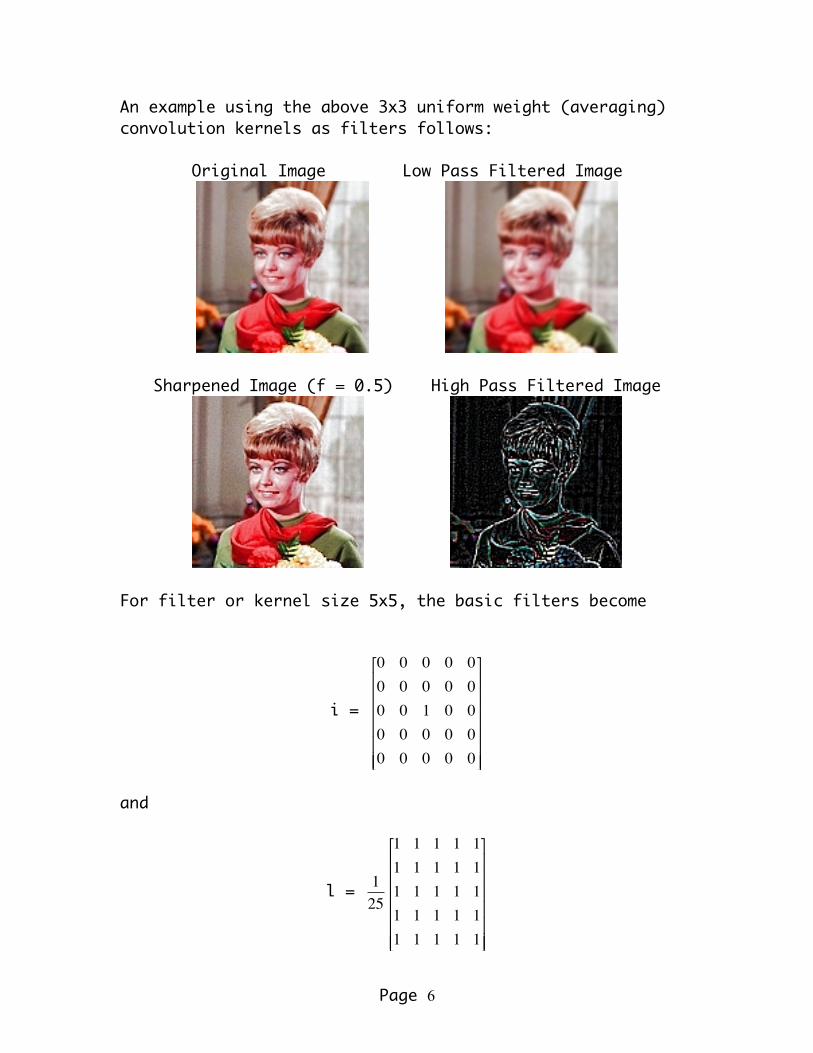
An example using the above 3x3 uniform weight (averaging) convolution kernels as filters follows:

Original Image Low Pass Filtered Image

Sharpened Image (f = 0.5) High Pass Filtered Image

For filter or kernel size 5x5, the basic filters become

i =

€

0 0 0 0 00 0 0 0 00 0 1 0 00 0 0 0 00 0 0 0 0

⎡

⎣

⎢ ⎢ ⎢ ⎢ ⎢ ⎢

⎤

⎦

⎥ ⎥ ⎥ ⎥ ⎥ ⎥

and

l =

€

125

€

1 1 1 1 11 1 1 1 11 1 1 1 11 1 1 1 11 1 1 1 1

⎡

⎣

⎢ ⎢ ⎢ ⎢ ⎢ ⎢

⎤

⎦

⎥ ⎥ ⎥ ⎥ ⎥ ⎥

Page 7

so that

h =

€

125

€

−1 −1 −1 −1 −1−1 −1 −1 −1 −1−1 −1 24 −1 −1−1 −1 −1 −1 −1−1 −1 −1 −1 −1

⎡

⎣

⎢ ⎢ ⎢ ⎢ ⎢ ⎢

⎤

⎦

⎥ ⎥ ⎥ ⎥ ⎥ ⎥

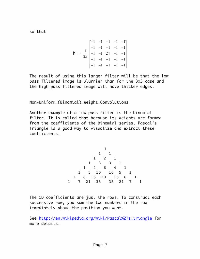
The result of using this larger filter will be that the low pass filtered image is blurrier than for the 3x3 case and the high pass filtered image will have thicker edges. Non-Uniform (Binomial) Weight Convolutions Another example of a low pass filter is the binomial filter. It is called that because its weights are formed from the coefficients of the binomial series. Pascal’s Triangle is a good way to visualize and extract these coefficients.

1 1 1 1 2 1 1 3 3 1 1 4 6 4 1 1 5 10 10 5 1 1 6 15 20 15 6 1 1 7 21 35 35 21 7 1 The 1D coefficients are just the rows. To construct each successive row, you sum the two numbers in the row immediately above the position you want. See http://en.wikipedia.org/wiki/Pascal%27s_triangle for more details.

Page 8

The first two odd sized series are:

1 2 1

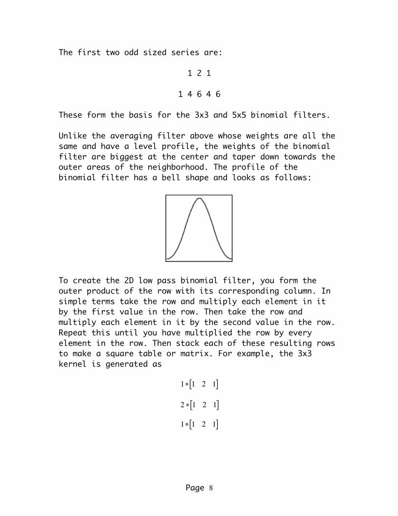
1 4 6 4 6 These form the basis for the 3x3 and 5x5 binomial filters. Unlike the averaging filter above whose weights are all the same and have a level profile, the weights of the binomial filter are biggest at the center and taper down towards the outer areas of the neighborhood. The profile of the binomial filter has a bell shape and looks as follows:

To create the 2D low pass binomial filter, you form the outer product of the row with its corresponding column. In simple terms take the row and multiply each element in it by the first value in the row. Then take the row and multiply each element in it by the second value in the row. Repeat this until you have multiplied the row by every element in the row. Then stack each of these resulting rows to make a square table or matrix. For example, the 3x3 kernel is generated as

€

1∗ 1 2 1[ ]

€

2 ∗ 1 2 1[ ]

€

1∗ 1 2 1[ ]

Page 9

When multiplied and stacked, it becomes

l =

€

116

€

1 2 12 4 21 2 1

⎡

⎣

⎢ ⎢ ⎢

⎤

⎦

⎥ ⎥ ⎥

Similarly, the 5x5 low pass binomial filter becomes

l =

€

1256

€

1 4 6 4 14 16 24 16 46 24 36 24 64 16 24 16 41 4 6 4 1

⎡

⎣

⎢ ⎢ ⎢ ⎢ ⎢ ⎢

⎤

⎦

⎥ ⎥ ⎥ ⎥ ⎥ ⎥

To get the high pass filter, we use the same formula as before, namely, h = i – l. Thus for the 3x3 case, we get

h =

€

116

€

−1 −2 −1−2 12 −2−1 −2 −1

⎡

⎣

⎢ ⎢ ⎢

⎤

⎦

⎥ ⎥ ⎥

and the sharpening filter becomes

s =

€

116

€

− f −2 f − f−2 f (16 − f ) −2 f− f −2 f − f

⎡

⎣

⎢ ⎢ ⎢

⎤

⎦

⎥ ⎥ ⎥

Page 10

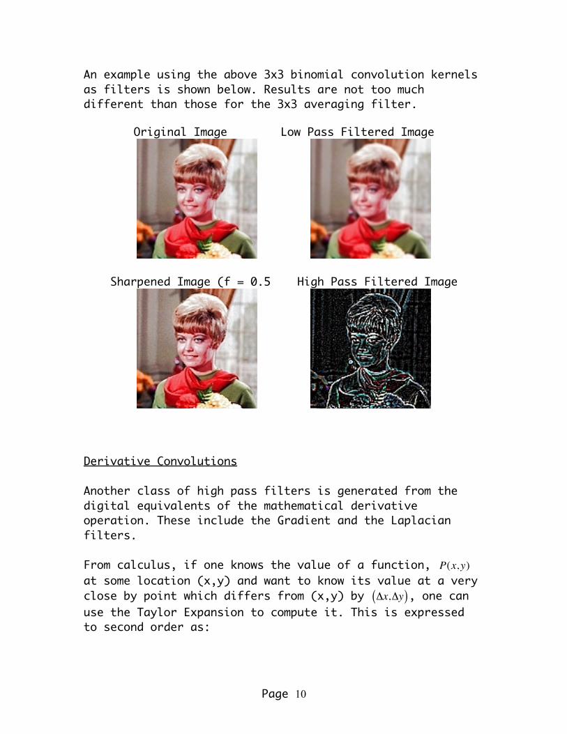
An example using the above 3x3 binomial convolution kernels as filters is shown below. Results are not too much different than those for the 3x3 averaging filter.

Original Image Low Pass Filtered Image

Sharpened Image (f = 0.5 High Pass Filtered Image

Derivative Convolutions Another class of high pass filters is generated from the digital equivalents of the mathematical derivative operation. These include the Gradient and the Laplacian filters. From calculus, if one knows the value of a function,

€

P(x,y) at some location (x,y) and want to know its value at a very close by point which differs from (x,y) by

€

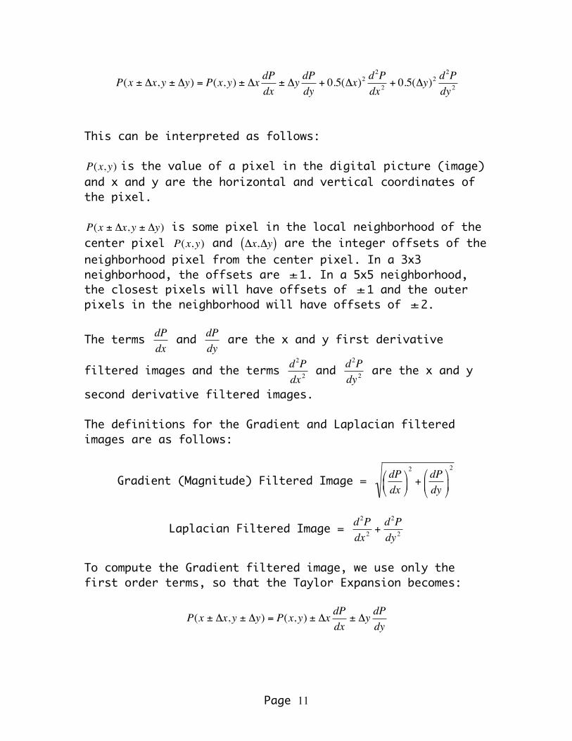
Δx,Δy( ), one can use the Taylor Expansion to compute it. This is expressed to second order as:

Page 11

€

P(x ± Δx,y ± Δy) = P(x,y) ± Δx dPdx

± Δy dPdy

+ 0.5(Δx)2 d2Pdx 2

+ 0.5(Δy)2 d2Pdy 2

This can be interpreted as follows:

€

P(x,y) is the value of a pixel in the digital picture (image) and x and y are the horizontal and vertical coordinates of the pixel.

€

P(x ± Δx,y ± Δy) is some pixel in the local neighborhood of the center pixel

€

P(x,y) and

€

Δx,Δy( ) are the integer offsets of the neighborhood pixel from the center pixel. In a 3x3 neighborhood, the offsets are

€

±1. In a 5x5 neighborhood, the closest pixels will have offsets of

€

±1 and the outer pixels in the neighborhood will have offsets of

€

±2. The terms

€

dPdx

and

€

dPdy

are the x and y first derivative

filtered images and the terms

€

d2Pdx 2

and

€

d2Pdy 2

are the x and y

second derivative filtered images. The definitions for the Gradient and Laplacian filtered images are as follows:

Gradient (Magnitude) Filtered Image =

€

dPdx

⎛ ⎝ ⎜

⎞ ⎠ ⎟

2

+dPdy

⎛

⎝ ⎜

⎞

⎠ ⎟

2

Laplacian Filtered Image =

€

d2Pdx 2

+d2Pdy 2

To compute the Gradient filtered image, we use only the first order terms, so that the Taylor Expansion becomes:

€

P(x ± Δx,y ± Δy) = P(x,y) ± Δx dPdx

± Δy dPdy

Page 12

Lets look at the 8 pixels in the neighborhood of

€

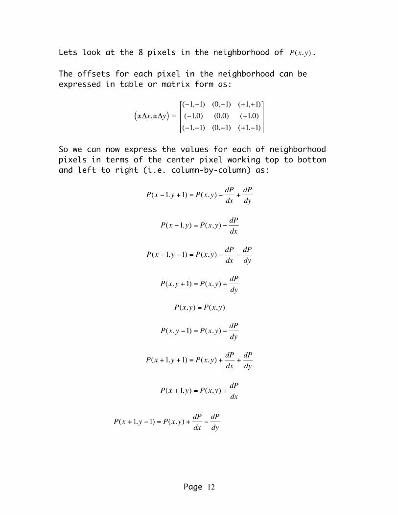
P(x,y). The offsets for each pixel in the neighborhood can be expressed in table or matrix form as:

€

±Δx,±Δy( ) =

€

(−1,+1) (0,+1) (+1,+1)(−1,0) (0,0) (+1,0)(−1,−1) (0,−1) (+1,−1)

⎡

⎣

⎢ ⎢ ⎢

⎤

⎦

⎥ ⎥ ⎥

So we can now express the values for each of neighborhood pixels in terms of the center pixel working top to bottom and left to right (i.e. column-by-column) as:

€

P(x −1,y +1) = P(x,y) − dPdx

+dPdy

€

P(x −1,y) = P(x,y) − dPdx

€

P(x −1,y −1) = P(x,y) − dPdx

−dPdy

€

P(x,y +1) = P(x,y) +dPdy

€

P(x,y) = P(x,y)

€

P(x,y −1) = P(x,y) − dPdy

€

P(x +1,y +1) = P(x,y) +dPdx

+dPdy

€

P(x +1,y) = P(x,y) +dPdx

€

P(x +1,y −1) = P(x,y) +dPdx

−dPdy

€

Page 13

Lets start by looking at the middle column (equations 4, 5 and 6 above). We note that none of them include

€

dPdx

.

Next look at the left column of neighborhood pixels (equations 1, 2 and 3 above). If we add these up, we get

Left column of 3 pixels =

€

3P(x,y) − dPdx

Similarly for the right column of 3 pixels (equations 7, 8 and 9 above), we get

Right column of 3 pixels =

€

3P(x,y) +dPdx

If we subtract the left column from the right column we get

(Right column of pixels) – (Left column of pixels) =

€

dPdx

This equation tells us that the left and right columns are the only pixels that make up this derivative. Thus the pixels in the center column must each have a value of zero as none of these pixels contribute to the derivative. This equation along with the equation for the left column of pixels tells us that the sign of the left column must be negative. Similarly, this equation along with the equation for the right column of pixels tells us that the sign of the right column must be positive. Nothing in these equations tells us what exact values to use for the weights of the left and right columns, except they must be equal and opposite sign across a row. The simplest assumption is to weight them equally.

Page 14

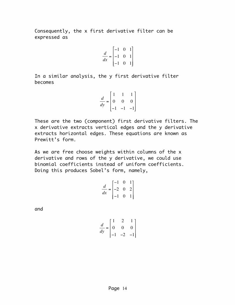
Consequently, the x first derivative filter can be expressed as

€

ddx

=

−1 0 1−1 0 1−1 0 1

⎡

⎣

⎢ ⎢ ⎢

⎤

⎦

⎥ ⎥ ⎥

In a similar analysis, the y first derivative filter becomes

€

ddy

=

1 1 10 0 0−1 −1 −1

⎡

⎣

⎢ ⎢ ⎢

⎤

⎦

⎥ ⎥ ⎥

These are the two (component) first derivative filters. The x derivative extracts vertical edges and the y derivative extracts horizontal edges. These equations are known as Prewitt’s form. As we are free choose weights within columns of the x derivative and rows of the y derivative, we could use binomial coefficients instead of uniform coefficients. Doing this produces Sobel’s form, namely,

€

ddx

=

−1 0 1−2 0 2−1 0 1

⎡

⎣

⎢ ⎢ ⎢

⎤

⎦

⎥ ⎥ ⎥

and

€

ddy

=

1 2 10 0 0−1 −2 −1

⎡

⎣

⎢ ⎢ ⎢

⎤

⎦

⎥ ⎥ ⎥

Page 15

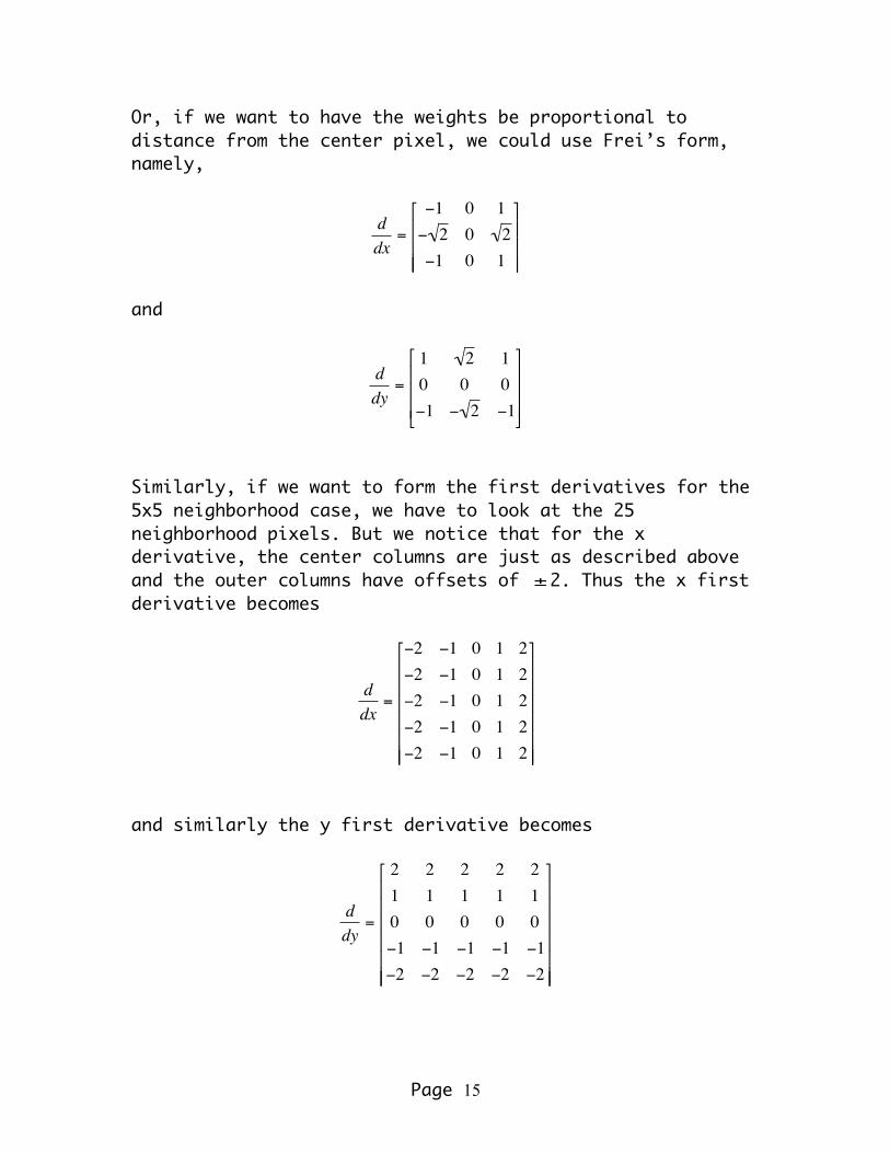
Or, if we want to have the weights be proportional to distance from the center pixel, we could use Frei’s form, namely,

€

ddx

=

−1 0 1− 2 0 2−1 0 1

⎡

⎣

⎢ ⎢ ⎢

⎤

⎦

⎥ ⎥ ⎥

and

€

ddy

=

1 2 10 0 0−1 − 2 −1

⎡

⎣

⎢ ⎢ ⎢

⎤

⎦

⎥ ⎥ ⎥

Similarly, if we want to form the first derivatives for the 5x5 neighborhood case, we have to look at the 25 neighborhood pixels. But we notice that for the x derivative, the center columns are just as described above and the outer columns have offsets of

€

±2. Thus the x first derivative becomes

€

ddx

=

−2 −1 0 1 2−2 −1 0 1 2−2 −1 0 1 2−2 −1 0 1 2−2 −1 0 1 2

⎡

⎣

⎢ ⎢ ⎢ ⎢ ⎢ ⎢

⎤

⎦

⎥ ⎥ ⎥ ⎥ ⎥ ⎥

and similarly the y first derivative becomes

€

ddy

=

2 2 2 2 21 1 1 1 10 0 0 0 0−1 −1 −1 −1 −1−2 −2 −2 −2 −2

⎡

⎣

⎢ ⎢ ⎢ ⎢ ⎢ ⎢

⎤

⎦

⎥ ⎥ ⎥ ⎥ ⎥ ⎥

Page 16

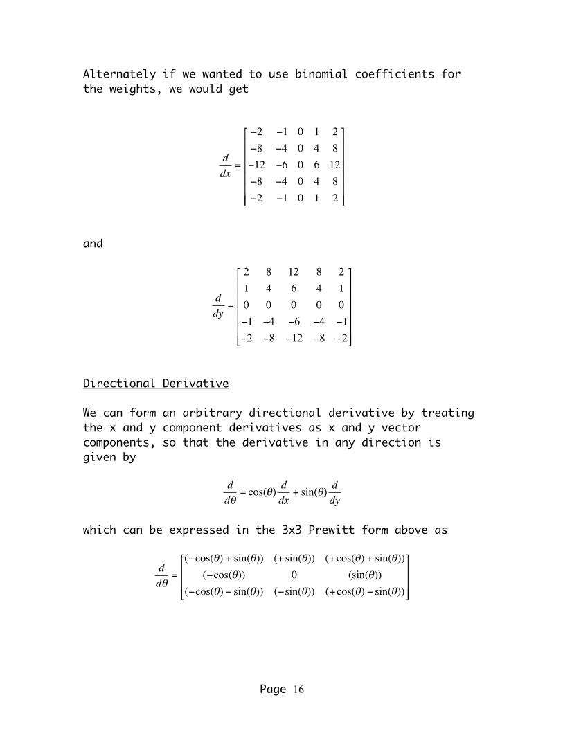
Alternately if we wanted to use binomial coefficients for the weights, we would get

€

ddx

=

−2 −1 0 1 2−8 −4 0 4 8−12 −6 0 6 12−8 −4 0 4 8−2 −1 0 1 2

⎡

⎣

⎢ ⎢ ⎢ ⎢ ⎢ ⎢

⎤

⎦

⎥ ⎥ ⎥ ⎥ ⎥ ⎥

and

€

ddy

=

2 8 12 8 21 4 6 4 10 0 0 0 0−1 −4 −6 −4 −1−2 −8 −12 −8 −2

⎡

⎣

⎢ ⎢ ⎢ ⎢ ⎢ ⎢

⎤

⎦

⎥ ⎥ ⎥ ⎥ ⎥ ⎥

Directional Derivative We can form an arbitrary directional derivative by treating the x and y component derivatives as x and y vector components, so that the derivative in any direction is given by

€

ddθ

= cos(θ) ddx

+ sin(θ) ddy

which can be expressed in the 3x3 Prewitt form above as

€

ddθ

=

(−cos(θ) + sin(θ)) (+ sin(θ)) (+cos(θ) + sin(θ))(−cos(θ)) 0 (sin(θ))

(−cos(θ) − sin(θ)) (−sin(θ)) (+cos(θ) − sin(θ))

⎡

⎣

⎢ ⎢ ⎢

⎤

⎦

⎥ ⎥ ⎥

Page 17

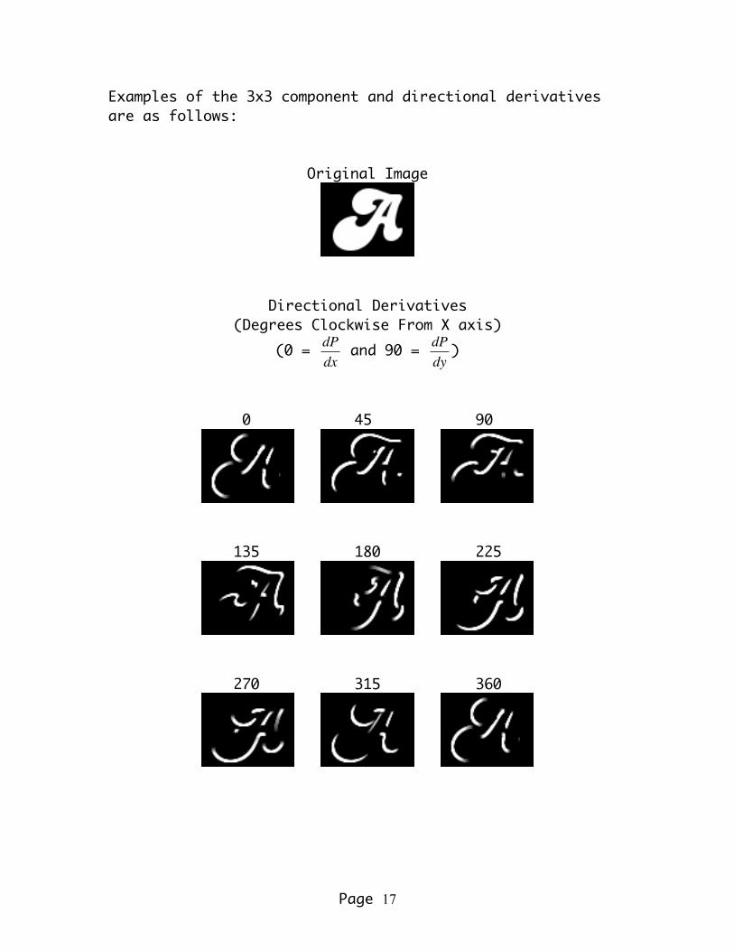
Examples of the 3x3 component and directional derivatives are as follows:

Original Image

Directional Derivatives (Degrees Clockwise From X axis)

(0 =

€

dPdx

and 90 =

€

dPdy

)

0 45 90

135 180 225

270 315 360

Page 18

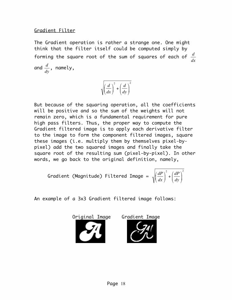
Gradient Filter The Gradient operation is rather a strange one. One might think that the filter itself could be computed simply by forming the square root of the sum of squares of each of

€

ddx

and

€

ddy, namely,

€

ddx⎛ ⎝ ⎜

⎞ ⎠ ⎟

2

+ddy⎛

⎝ ⎜

⎞

⎠ ⎟

2

But because of the squaring operation, all the coefficients will be positive and so the sum of the weights will not remain zero, which is a fundamental requirement for pure high pass filters. Thus, the proper way to compute the Gradient filtered image is to apply each derivative filter to the image to form the component filtered images, square these images (i.e. multiply them by themselves pixel-by-pixel) add the two squared images and finally take the square root of the resulting sum (pixel-by-pixel). In other words, we go back to the original definition, namely,

Gradient (Magnitude) Filtered Image =

€

dPdx

⎛ ⎝ ⎜

⎞ ⎠ ⎟

2

+dPdy

⎛

⎝ ⎜

⎞

⎠ ⎟

2

An example of a 3x3 Gradient filtered image follows:

Original Image Gradient Image

Page 19

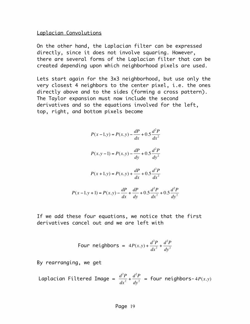
Laplacian Convolutions On the other hand, the Laplacian filter can be expressed directly, since it does not involve squaring. However, there are several forms of the Laplacian filter that can be created depending upon which neighborhood pixels are used. Lets start again for the 3x3 neighborhood, but use only the very closest 4 neighbors to the center pixel, i.e. the ones directly above and to the sides (forming a cross pattern). The Taylor expansion must now include the second derivatives and so the equations involved for the left, top, right, and bottom pixels become

€

P(x −1,y) = P(x,y) − dPdx

+ 0.5 d2Pdx 2

€

P(x,y −1) = P(x,y) − dPdy

+ 0.5 d2Pdy 2

€

P(x +1,y) = P(x,y) +dPdx

+ 0.5 d2Pdx 2

€

P(x −1,y +1) = P(x,y) − dPdx

+dPdy

+ 0.5 d2Pdx 2

+ 0.5 d2Pdy 2

If we add these four equations, we notice that the first derivatives cancel out and we are left with

Four neighbors =

€

4P(x,y) +d2Pdx 2

+d2Pdy 2

By rearranging, we get

Laplacian Filtered Image =

€

d2Pdx 2

+d2Pdy 2

= four neighbors-

€

4P(x,y)

Page 20

Or in filter form

Laplacian Filter =

€

d2

dx 2+d2

dy 2 =

€

0 1 01 −4 10 1 0

⎡

⎣

⎢ ⎢ ⎢

⎤

⎦

⎥ ⎥ ⎥

However, we usually express this filter as its negative so that, when combined with the original image to produce sharpening, we get the polarity of the edges that looks the most realistic. Either way, the sum of the weights is still zero. Thus we have

4-neighbor Laplacian Filter =

€

d2

dx 2+d2

dy 2 =

€

0 −1 0−1 4 −10 −1 0

⎡

⎣

⎢ ⎢ ⎢

⎤

⎦

⎥ ⎥ ⎥

If we do the same with all 8 neighbors in the 3x3 neighborhood, we get

8-neighbor Laplacian Filter =

€

d2

dx 2+d2

dy 2 =

€

−1 −1 −1−1 8 −1−1 −1 −1

⎡

⎣

⎢ ⎢ ⎢

⎤

⎦

⎥ ⎥ ⎥

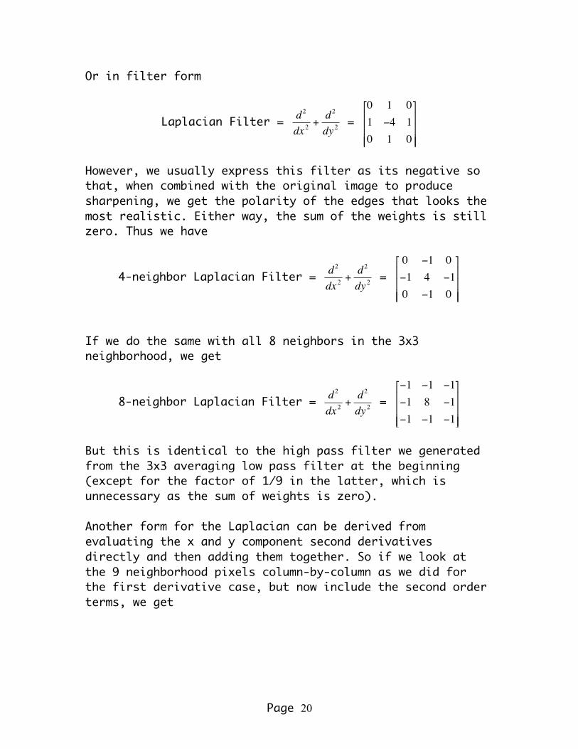
But this is identical to the high pass filter we generated from the 3x3 averaging low pass filter at the beginning (except for the factor of 1/9 in the latter, which is unnecessary as the sum of weights is zero). Another form for the Laplacian can be derived from evaluating the x and y component second derivatives directly and then adding them together. So if we look at the 9 neighborhood pixels column-by-column as we did for the first derivative case, but now include the second order terms, we get

Page 21

€

P(x −1,y +1) = P(x,y) − dPdx

+dPdy

+ 0.5 d2Pdx 2

+ 0.5 d2Pdy 2

€

P(x −1,y) = P(x,y) − dPdx

+ 0.5 d2Pdx 2

€

P(x −1,y −1) = P(x,y) − dPdx

−dPdy

+ 0.5 d2Pdx 2

+ 0.5 d2Pdy 2

€

P(x,y +1) = P(x,y) +dPdy

+ 0.5 d2Pdy 2

€

P(x,y) = P(x,y)

€

P(x,y −1) = P(x,y) − dPdy

+ 0.5 d2Pdy 2

€

P(x +1,y +1) = P(x,y) +dPdx

+dPdy

+ 0.5 d2Pdx 2

+ 0.5 d2Pdy 2

€

P(x +1,y) = P(x,y) +dPdx

+ 0.5 d2Pdx 2

€

P(x +1,y −1) = P(x,y) +dPdx

−dPdy

+ 0.5 d2Pdx 2

+ 0.5 d2Pdy 2

If we add the first 3 equations with the last 3 equations, we notice that all the first order x and y derivatives cancel out and we are left with

sum of left and right column pixels =

€

6P(x,y) + 3 d2Pdx 2

+ 2 d2Pdy 2

Page 22

If we then sum the middle column pixels leaving out the center pixel, the first order y derivatives cancel and we get

top and bottom middle column pixels =

€

2P(x,y) +d2Pdy 2

If we subtract twice this last equation from the previous equation, we get

6 side – 2*(top & bottom middle) pixels =

€

2P(x,y) + 3 d2Pdx 2

By rearranging, we get

€

d2Pdx 2

= (left & right columns – 2*middle top/bottom pixels)/3

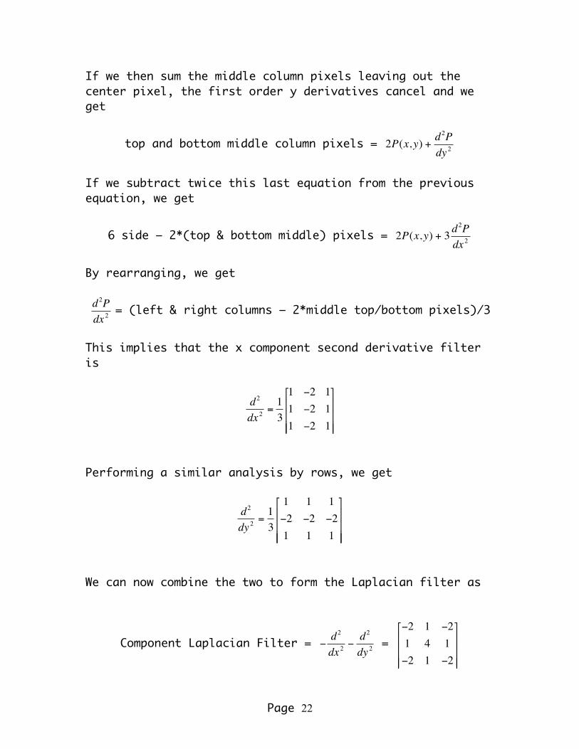
This implies that the x component second derivative filter is

€

d2

dx 2=13

1 −2 11 −2 11 −2 1

⎡

⎣

⎢ ⎢ ⎢

⎤

⎦

⎥ ⎥ ⎥

Performing a similar analysis by rows, we get

€

d2

dy 2=13

1 1 1−2 −2 −21 1 1

⎡

⎣

⎢ ⎢ ⎢

⎤

⎦

⎥ ⎥ ⎥

We can now combine the two to form the Laplacian filter as

Component Laplacian Filter =

€

−d2

dx 2−d2

dy 2 =

€

−2 1 −21 4 1−2 1 −2

⎡

⎣

⎢ ⎢ ⎢

⎤

⎦

⎥ ⎥ ⎥

Page 23

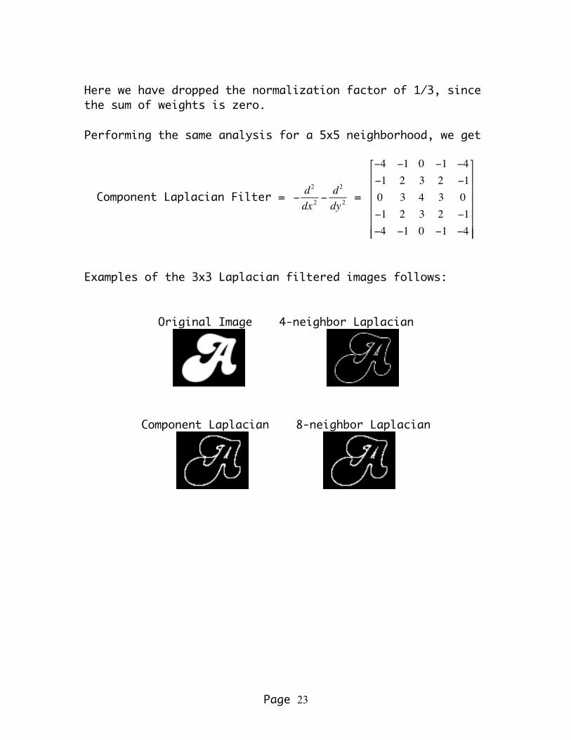
Here we have dropped the normalization factor of 1/3, since the sum of weights is zero. Performing the same analysis for a 5x5 neighborhood, we get

Component Laplacian Filter =

€

−d2

dx 2−d2

dy 2 =

€

−4 −1 0 −1 −4−1 2 3 2 −10 3 4 3 0−1 2 3 2 −1−4 −1 0 −1 −4

⎡

⎣

⎢ ⎢ ⎢ ⎢ ⎢ ⎢

⎤

⎦

⎥ ⎥ ⎥ ⎥ ⎥ ⎥

Examples of the 3x3 Laplacian filtered images follows:

Original Image 4-neighbor Laplacian

Component Laplacian 8-neighbor Laplacian

Page 24

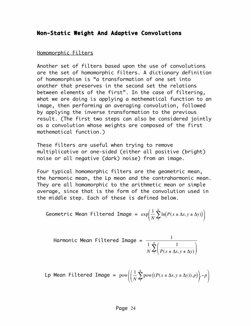
Non-Static Weight And Adaptive Convolutions Homomorphic Filters Another set of filters based upon the use of convolutions are the set of homomorphic filters. A dictionary definition of homomorphism is “a transformation of one set into another that preserves in the second set the relations between elements of the first”. In the case of filtering, what we are doing is applying a mathematical function to an image, then performing an averaging convolution, followed by applying the inverse transformation to the previous result. (The first two steps can also be considered jointly as a convolution whose weights are composed of the first mathematical function.) These filters are useful when trying to remove multiplicative or one-sided (either all positive (bright) noise or all negative (dark) noise) from an image. Four typical homomorphic filters are the geometric mean, the harmonic mean, the Lp mean and the contraharmonic mean. They are all homomorphic to the arithmetic mean or simple average, since that is the form of the convolution used in the middle step. Each of these is defined below.

Geometric Mean Filtered Image =

€

exp 1N

ln1

N

∑ P(x ± Δx,y ± Δy)( )⎛

⎝ ⎜

⎞

⎠ ⎟

Harmonic Mean Filtered Image =

€

11N

1P(x ± Δx,y ± Δy)⎛

⎝ ⎜

⎞

⎠ ⎟

1

N

∑

€

Lp Mean Filtered Image =

€

pow 1N

pow (P(x ± Δx,y ± Δy)), p( )1

N

∑⎛

⎝ ⎜

⎞

⎠ ⎟ ,−p

⎛

⎝ ⎜

⎞

⎠ ⎟

Page 25

Contraharmonic Filtered Image =

€

pow (P(x ± Δx,y ± Δy)), p +1( )1

N

∑

pow (P(x ± Δx,y ± Δy)), p( )1

N

∑

Here N is the number of pixels in the neighborhood (convolution size), ln is the natural logarithm function, exp is the exponentiation function, pow is the function that raises the value of the pixel to some exponent and p is the exponent. For the Lp mean and contraharmonic mean, use positive values for p when the image has one-sided dark noise and use negative values for p when the image has one-sided bright noise. In ImageMagick, we would do the following for a 3x3 neighborhood: Geometric Mean Filtering: convert infile -fx "ln(u+1)" \

-convolve "1,1,1,1,1,1,1,1,1" \ -fx "exp(u)-1" outfile

Since –fx uses pixel values in the range of 0-1, and ln(1)=0 and ln(0)=-infinity, all results would be less than or equal to zero and not acceptable. Thus we add one before doing the ln and subtract one after doing the exp operations to keep the values for fx acceptable.

Page 26

Harmonic Mean Filtering: convert infile -fx "1/(u+1)" \

-convolve "1,1,1,1,1,1,1,1,1" \ -fx "(1/u)-1" outfile

Again we have added and subtracted one to avoid the case when a pixel value is zero since 1/0 will be infinite. Lp Mean Filtering: For positive values of p, convert infile -fx "pow(u,$p)" \

-convolve "1,1,1,1,1,1,1,1,1" \ -fx "pow(u,$ip)" outfile

And for negative values of p, we can reverse the polarity of the image, use positive values of p and reverse the polarity back. This avoids the 1/0 problem again convert infile -negate -fx "pow(u,$p)" \

-convolve "1,1,1,1,1,1,1,1,1" \ -negate outfile

Contraharmonic Filtering: For positive values of p, convert \

\( infile -fx "(pow((u),$p1))" \ -convolve "1,1,1,1,1,1,1,1,1" \) \ \( infile -fx "(pow((u),$p))" \ -convolve "1,1,1,1,1,1,1,1,1" \) \ -fx "(u/v)" outfile

Page 27

and for negative p, we use the same polarity reversal technique, convert \

\( infile -negate -fx "(pow((u),$p1))" \ -convolve "1,1,1,1,1,1,1,1,1" \) \ \( infile -negate -fx "(pow((u),$p))" \ -convolve "1,1,1,1,1,1,1,1,1" \) \ -fx "(u/v)" -negate outfile

Page 28

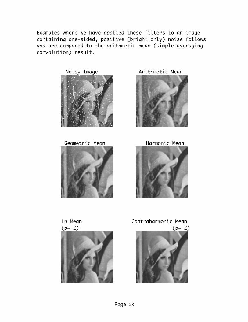
Examples where we have applied these filters to an image containing one-sided, positive (bright only) noise follows and are compared to the arithmetic mean (simple averaging convolution) result.

Noisy Image Arithmetic Mean

Geometric Mean Harmonic Mean

Lp Mean Contraharmonic Mean (p=-2) (p=-2)

Page 29

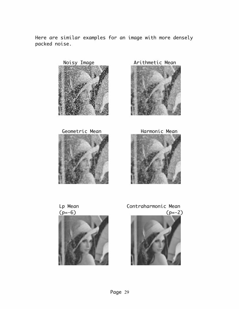
Here are similar examples for an image with more densely packed noise.

Noisy Image Arithmetic Mean

Geometric Mean Harmonic Mean

Lp Mean Contraharmonic Mean (p=-6) (p=-2)

Page 30

Statistical Filters Another type of filter replaces each pixel in an image with some statistical measure involving the pixels in the local neighborhood of that pixel. Two filters in this category are the median filter and the Kth nearest neighbors filter. With the median filter, all the pixels in the neighborhood are ranked by intensity level and the center pixel is replaced by that pixel which is mid-way in ranking. Median filtering is generally one of the better filtering techniques. Nevertheless, it does cause some blurring, although less than a simple average. In ImageMagick, this is done as follows for a 3x3 neighborhood (as indicated by the radius value of 1):

convert infile –median 1 outfile With the Kth nearest neighbors filter, the intensity value of each pixel in the neighborhood is compared with that of the center pixel and only those k number of pixels whose values are closest to that of the center pixel are averaged. One example is the 1st nearest neighbor filter. It simply replaces each pixel in the image with that one pixel in its neighborhood whose value is closest to its own value. In ImageMagick, this is done as follows for a 3x3 neighborhood (as indicated by the radius value of 1):

convert infile –noise 1 outfile

Page 31

Another filter simply throws out 2 pixels, one with the greatest positive difference from the center pixel and the other with the greatest negative difference from the center pixel and averages the rest. For a 3x3 neighborhood, this is the 7th nearest neighbor filter. In ImageMagick, this is a bit more difficult (and slow), but can be done as follows for a 3x3 neighborhood and K=7: pixels="aa=p[-1,-1]; ab=p[0,-1]; ac=p[+1,-1]; ba=p[-1,0]; bb=p[0,0]; bc=p[+1,0]; ca=p[-1,+1]; cb=p[0,+1]; cc=p[+1,+1];" tot="((aa)+(ab)+(ac)+(ba)+(bb)+(bc)+(ca)+(cb)+(cc))" min="min(min(min(min(min(min(min(min(aa,ab),ac),ba),bb),bc),ca),cb),cc)" max="max(max(max(max(max(max(max(max(aa,ab),ac),ba),bb),bc),ca),cb),cc)" convert infile -fx "$pixels u=($tot-$max-$min)/7" outfile Another statistical filter is the distance-weighted average. This is equivalent to a convolution whose coefficients (weights) change dynamically according to some measure of intensity difference (distance) from that of the center pixels. Typically, it excludes the center pixel from the average. Two variations are the linear distance weighted average and the inverse distance weighted average. In the former, the simple difference in intensity levels is used as the distance measure. Smaller differences are weighted higher. In the latter, the inverse of the difference is used as the distance measure, so that closer values are again weighted higher.

Page 32

In ImageMagick, these are even slower, but can be done as follows for a 3x3 neighborhood: Linear Distance Weighting: ref=1.000001 #to avoid a divide by zero pixels="aa=p[-1,-1]; ab=p[0,-1]; ac=p[+1,-1]; ba=p[-1,0]; bb=p[0,0]; bc=p[+1,0]; ca=p[-1,+1]; cb=p[0,+1]; cc=p[+1,+1];" wts="waa=$ref-(abs(aa-bb)); wab=$ref-(abs(ab-bb)); wac=$ref-(abs(ac-bb)); wba=$ref-(abs(ba-bb)); wbc=$ref-(abs(bc-bb)); wca=$ref-(abs(ca-bb)); wcb=$ref-(abs(cb-bb)); wcc=$ref-(abs(cc-bb));" sum="((waa*aa)+(wab*ab)+(wac*ac)+(wba*ba)+(wbc*bc)+(wca*ca)+(wcb*cb)+(wcc*cc))" wtSum="(waa+wab+wac+wba+wbc+wca+wcb+wcc)" convert $tmpA -fx "$pixels $wts u=($sum/$wtSum)" $outfile Inverse Distance Weighting: pixels="aa=p[-1,-1]; ab=p[0,-1]; ac=p[+1,-1]; ba=p[-1,0]; bb=p[0,0]; bc=p[+1,0]; ca=p[-1,+1]; cb=p[0,+1]; cc=p[+1,+1];" wts="waa=(1/(abs(aa-bb)+(abs(aa-bb)==0))); wab=(1/(abs(ab-bb)+(abs(ab-bb)==0))); wac=(1/(abs(ac-bb)+(abs(ac-bb)==0))); wba=(1/(abs(ba-bb)+(abs(ba-bb)==0))); wbc=(1/(abs(bc-bb)+(abs(bc-bb)==0))); wca=(1/(abs(ca-bb)+(abs(ca-bb)==0))); wcb=(1/(abs(cb-bb)+(abs(cb-bb)==0))); wcc=(1/(abs(cc-bb)+(abs(cc-bb)==0)));" sum="((waa*aa)+(wab*ab)+(wac*ac)+(wba*ba)+(wbc*bc)+(wca*ca)+(wcb*cb)+(wcc*cc))" wtSum="(waa+wab+wac+wba+wbc+wca+wcb+wcc)" convert $tmpA -fx "$pixels $wts u=($sum/$wtSum)" $outfile

Page 33

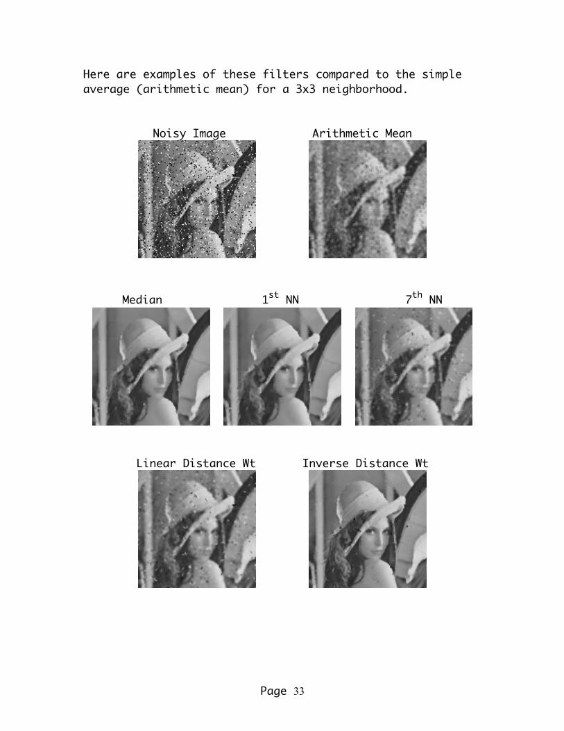
Here are examples of these filters compared to the simple average (arithmetic mean) for a 3x3 neighborhood.

Noisy Image Arithmetic Mean

Median 1st NN 7th NN

Linear Distance Wt Inverse Distance Wt

Page 34

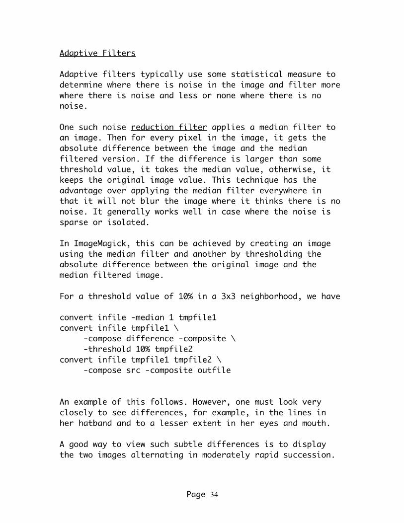
Adaptive Filters Adaptive filters typically use some statistical measure to determine where there is noise in the image and filter more where there is noise and less or none where there is no noise. One such noise reduction filter applies a median filter to an image. Then for every pixel in the image, it gets the absolute difference between the image and the median filtered version. If the difference is larger than some threshold value, it takes the median value, otherwise, it keeps the original image value. This technique has the advantage over applying the median filter everywhere in that it will not blur the image where it thinks there is no noise. It generally works well in case where the noise is sparse or isolated. In ImageMagick, this can be achieved by creating an image using the median filter and another by thresholding the absolute difference between the original image and the median filtered image. For a threshold value of 10% in a 3x3 neighborhood, we have convert infile -median 1 tmpfile1 convert infile tmpfile1 \

-compose difference -composite \ -threshold 10% tmpfile2

convert infile tmpfile1 tmpfile2 \ -compose src -composite outfile

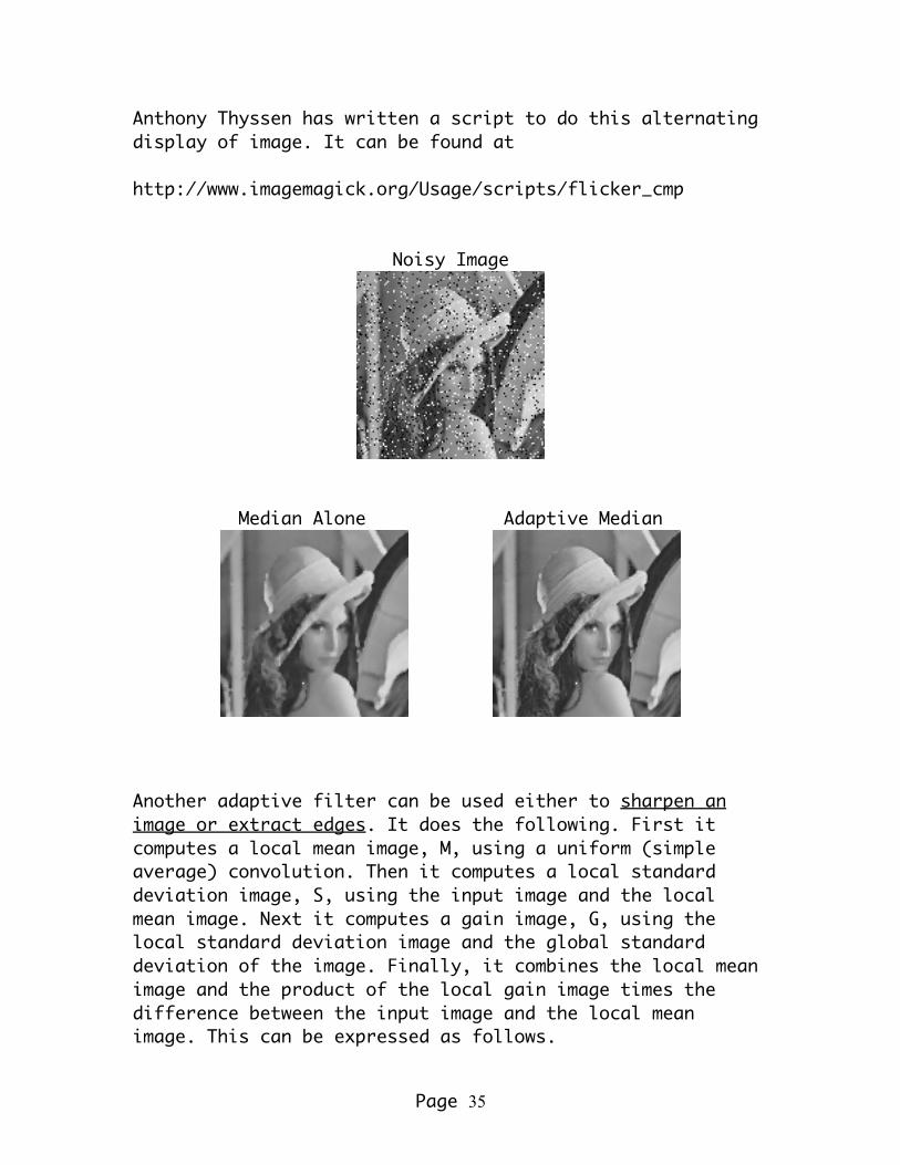
An example of this follows. However, one must look very closely to see differences, for example, in the lines in her hatband and to a lesser extent in her eyes and mouth. A good way to view such subtle differences is to display the two images alternating in moderately rapid succession.

Page 35

Anthony Thyssen has written a script to do this alternating display of image. It can be found at http://www.imagemagick.org/Usage/scripts/flicker_cmp

Noisy Image

Median Alone Adaptive Median

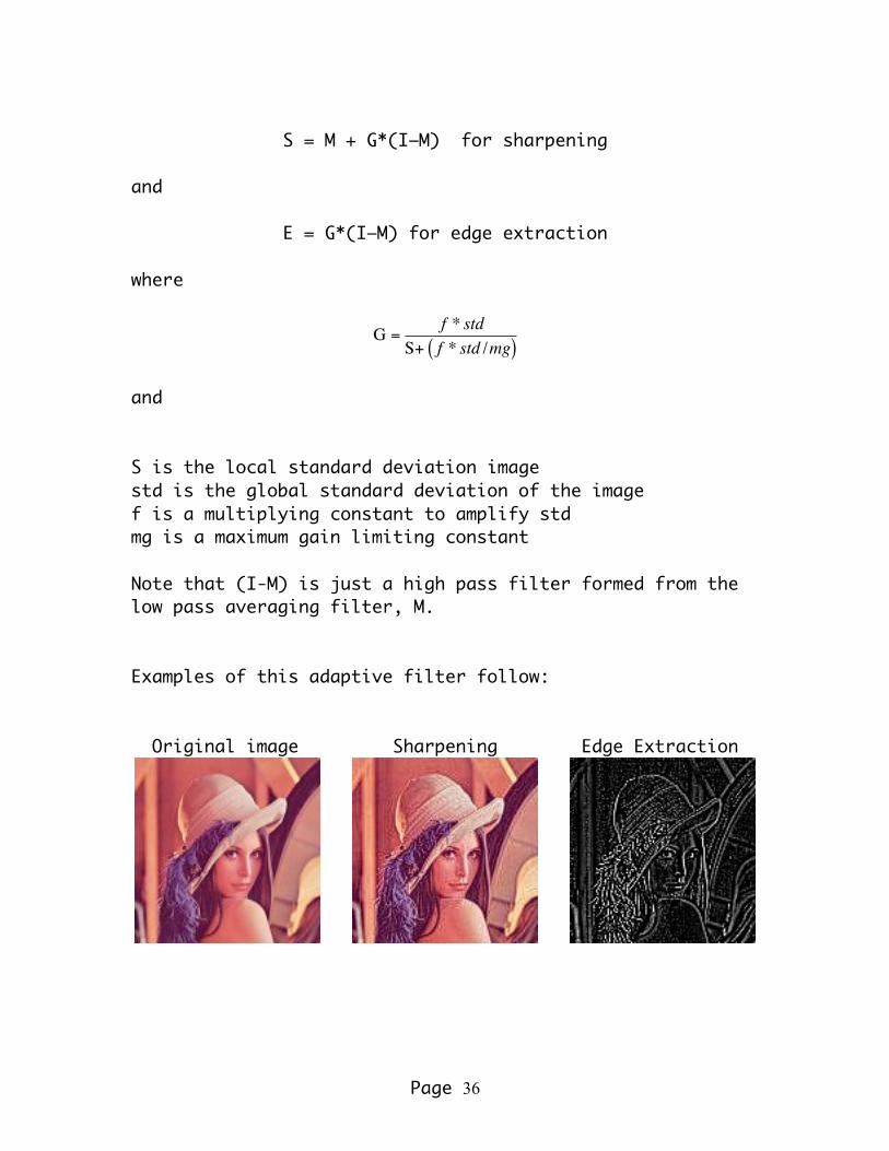
Another adaptive filter can be used either to sharpen an image or extract edges. It does the following. First it computes a local mean image, M, using a uniform (simple average) convolution. Then it computes a local standard deviation image, S, using the input image and the local mean image. Next it computes a gain image, G, using the local standard deviation image and the global standard deviation of the image. Finally, it combines the local mean image and the product of the local gain image times the difference between the input image and the local mean image. This can be expressed as follows.

Page 36

S = M + G*(I–M) for sharpening

and

E = G*(I–M) for edge extraction where

€

G =f * std

S+ f * std /mg( )

and S is the local standard deviation image std is the global standard deviation of the image f is a multiplying constant to amplify std mg is a maximum gain limiting constant Note that (I-M) is just a high pass filter formed from the low pass averaging filter, M. Examples of this adaptive filter follow: Original image Sharpening Edge Extraction

Page 37

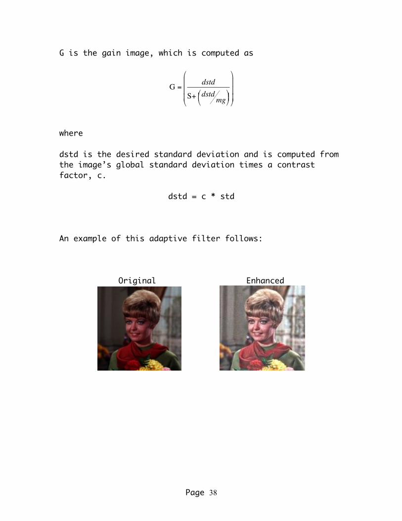
Adaptive filters can also be used to enhance the contrast and brightness of an image. The next filter does this using a concept that is very similar to the adaptive sharpening filter above. It computes both a local mean and standard deviation filtered image, except, rather than doing it at every pixel, it does in for blocks of pixels and then skips to the next block. This generates reduces size images which are then re-expanded smoothly back to the original image size. It then uses the expanded standard deviation image to compute a gain image that will be multiplied by the difference between the input image and the expanded mean image. The mean image, a desired mean value and the product of the gain times the difference between the input image and the mean image are then mixed together to produce the resulting contrast and brightness enhanced image. This can be expressed as follows:

R = f*dmean + (1-f)*b*M + G*(I–M) where R is the resulting enhanced image M is the re-expanded mean image S is the re-expanded standard deviation image I is the original image f is the mixing fraction, 0 <= f <= 1 dmean is the desired mean and is computed from the image’s global mean times a brightening factor, b.

dmean = b * mean and

Page 38

G is the gain image, which is computed as

€

G =dstd

S+ dstdmg

⎛ ⎝ ⎜ ⎞

⎠ ⎟

⎛

⎝

⎜ ⎜ ⎜

⎞

⎠

⎟ ⎟ ⎟

where dstd is the desired standard deviation and is computed from the image’s global standard deviation times a contrast factor, c.

dstd = c * std An example of this adaptive filter follows:

Original Enhanced

Page 39

Using ImageMagick, this picture would be processed as follows, where the block averaging size was 12.5% of the full picture, m=0.5, b=2, c=1.5 and mg=5 convert infile -filter box -resize 12.5% tmpMfile convert \( infile infile -compose multiply -composite \ -filter box -resize 12.5% \) \ \( tmpMfile tmpMfile -compose multiply -composite \) \ +swap -compose minus -composite -fx "sqrt(u)" tmpSfile convert tmpMfile -resize 800% tmpMEfile convert tmpSfile -resize 800% tmpSEfile dmean=`echo "scale=5; 2 * $mean / 1" | bc` dstd=`echo "scale=5; 1.5 * $std / 1" | bc` fdmean=`echo "scale=5; 0.5 * $dmean / 1" | bc` dsdmg=`echo "scale=5; $dstd / 5" | bc` bf=`echo "scale=5; 2 * (1 - 0.5) / 1" | bc` gain="gn=($dstd)/(u[2]+($dsdmg));" convert infile tmpMEfile tmpSEfile \ -fx "$gain ($fdmean)+($bf*v)+(gn*(u-v))" outfile