Embed Size (px)
Citation preview

Wireless Personal Communications 23: 253–281, 2002.© 2002 Kluwer Academic Publishers. Printed in the Netherlands.
Digital-to-Analog Conversion of Pulse AmplitudeModulated Systems Using Adaptive Quantization
GIRIDHAR D. MANDYAMNokia Research Center, 6000 Connection Drive, Irving, TX 75039, U.S.A.E-mail: [email protected]
Abstract. In this paper, a full analysis is presented on digital-to-analog conversion for pulse amplitude modulated(PAM) systems. By analyzing the cyclostationary nature of pulse-amplitude modulation (PAM) systems, twomethods of quantization are proposed – fixed and adaptive. Examples of this quantization analysis are providedfor the reverse link transmitter chain in a cdma2000 system, and for the baseband transmitter chain of an IS-136 system. In addition, the impact of D/A converter nonlinearity on resultant signal-to-noise ratio is analyzed.Simulations are provided which show that adaptive quantization provides performance benefits over fixed methodsin terms of adjacent channel power rejection (ACPR) and transmitter signal-to-noise ratio.
Keywords: pulse-amplitude modulation, digital-to-analog conversion, transceivers.
1. Introduction
Pulse-amplitude modulation (PAM) is a common transmission method used for digitalcommunications. PAM systems operate by passing information-bearing pulses through pulse-shaping filters to provide signals that are smoothed in time but band-limited in frequency. Asa result, PAM transmission methods are often employed in wireless communications systems,which are bandlimited in nature.
PAM signals possess cyclostationary characteristics [1]. This property of PAM signals maybe exploited in performing digital-to-analog conversion. In particular, one is interested in thescaling of the PAM signal prior to digital-to-analog conversion. Normally this scaling is afunction of the probability density function of the signal. In this work, the PAM probabilitydensity function (pdf) is derived with respect to typical digital pulse-shaping. As examples,the cdma2000 and IS-136 systems are considered for analysis of pdf-optimized quantizationwith respect to cyclostationarity.
Similar to the IS-95-B system, the cdma2000 system [2] specifies the use of channel aggre-gation on the reverse link. However, a feature of cdma2000 channel aggregation not presentin IS-95-B is the use of individual channel gain adjustment. These channel gain adjustmentsprovide enhanced performance for coherent reverse link reception and can be used for quality-of-service considerations for data services. However, channel gains result in power adjustmentof incoming data, which combined with pulse shaping, can dramatically affect resultant signalpower. As a result, the effective spurious free dynamic range (SFDR) may degrade if quan-tization effects due to digital-to-analog conversion are not taken into account [3, 4]. In thispaper, the D/A conversion issues for cdma2000 are analyzed, and quantization algorithms forscaling prior to the D/A converter are derived and simulated.
In addition, the IS-136 system [5] time-division multiple-access (TDMA) system alsoemploys pulse-amplitude modulation. This type of system is just as sensitive to the dynamic
254 Giridhar D. Mandyam
range of transceivers as the cdma2000 system. In this paper, the D/A conversion issues forthe uplink baseband IS-136 subsystem are analyzed, with quantization algorithms derived andsimulated in the same fashion as the cdma2000 systems.
2. Pulse-Amplitude Modulated Systems
Pulse amplitude-modulated (PAM) systems involve the transmission of pulse-shaped im-pulses. The amplitude of the impulses directly relates to the information that they are carrying.In general, a PAM signal may be expressed by the following expression [6]
y(t) =∞∑
n=−∞cnp(t − nT ) , (1)
where cn represents the amplitude of the nth impulse, and p(t) is the pulse-shaping waveform.In many modern digital radio systems, pulse-shaping is performed digitally. Two important
reasons for this are: (A) it is often easier to implement the desired pulse waveform digitallythan in the analog domain and (B) the pulse-shaping operation may be used to increasethe sampling rate. Reason (A) relates to several aspects of the pulse-shaping filter, includ-ing matched filtering at the receiver and spectral shaping for electromagnetic compatibility.Reason (B) relates directly to the D/A conversion process, where sampling frequency affectsthe ease of design of not only the converter but also the sampling image-rejection filter thatnormally follows the DAC.
Of particular interest are the statistical properties of the PAM signal prior to D/A con-version. If one can fully characterize the PAM signal statistics, one may design an optimalquantizer for the signal. This leads directly to minimizing the distortion introduced by theD/A conversion process.
Assume that the series of impulses may be represented in the discrete-time domain bythe signal x(n), which is the amplitude of the impulse at the discrete-time index n. If weassume that the pulse-shaping filter N-tap h(n) has a tap-spacing of 1/L times the time-intervalbetween impulses and that x(n) is 0 for n < 0, then a version of x(n) must be created byzero-insertion:
xe(n) =∞∑
k=−∞x(k)δ(n − kL) . (2)
This process of zero-insertion introduces spectral copies of the original signal x(n) [9]; theensuing pulse-shaping takes care of this and also introduces the desired pulse waveform. Thefinal pulse-shaped waveform may be represented by the following relationship:
y(n) = h(n) ∗ xe(n)
=N−1∑r=0
h(r)xe(n − r)
=∞∑k=0
N−1∑r=0
h(r)x(k)δ(n − r − kL) .
(3)
Digital-to-Analog Conversion of Pulse Amplitude Modulated Systems 255
This relationship may be simplified further by assuming that the pulse-shaping filter h(n) haslength N , and that N is an integer multiple of L:
y(a + cL) =NL −1∑r=0
h(rL + a)x(c − r) , (4)
where a is an integer such that 0 ≤ a < L and c is an integer such that c ≥ 0. As is thecase with PAM systems, it may be assumed that the signal x(n) is drawn from a finite lengthalphabet {ai} of length A. If the alphabet is uniformly distributed, the probability densityfunction of x(n) may be represented as
px(x) =A−1∑i=0
1
Aδ(x − ai) . (5)
In (5), δ( ) is the dirac-delta function. Even if the alphabet is not uniformly distributed, it canbe assumed that the signal x(n) is stationary, as its pdf does not vary in time. As can be seenby (4), the filtered-output signal y(n0) at time n0 is dependent on N/L consecutive values ofthe stationary random process x(n) and the N/L coefficients drawn from h(n0) to determinethis value. Thus the pdf of y(n) may be expressed as
py(a+cL) = f
N
L −1∑r=0
h(rL + a)x(c − r)
= py(a+dL)∀d, c , (6)
where f ( ) is the pdf of its argument, and d is an integer such that d ≥ 0. This relationshipdemonstrates the cyclostationary nature of y(n).
One may narrow the assumption on the structure of h(n) to being linear phase. Therefore,these filter coefficients are symmetric, i.e. h(r) = h(N − r − 1) for 0 ≤ r < N . Referring to(4), one may group each set of N/L coefficients into subsets of h(r):
hi = {h(i), h(L + i), . . . , h((N/L − 1)L + i)} 0 ≤ i < L . (7)
Taking advantage of the symmetry of the linear phase filter, one may rewrite each subset as
hi ={h(N − 1 − i), h(N − 1 − (L + i)), . . . ,
h(N − 1 − ((N/L − 1)L + i))
}0 ≤ i < L . (8)
This in turn may be rewritten as
hi ={h((N/L − 1)L + L − 1 − i), h((N/L − 2)L + L − 1 − i), . . . ,
h(L − 1 − i)
}
0 ≤ i < L .
(9)

256 Giridhar D. Mandyam
The expression of hi given in (9) is merely an order-reversal of hL−i−1. As a result, the pdf’sresulting from these two subsets should be equivalent. This may be seen from modifying (6):
py(a+cL) = f
N
L−1∑
r=0
h(rL + a)x(c − r)
= f
N
L−1∑
r=0
h(N − 1 − (rL + a))x(c − r)
= f
N
L−1∑
r=0
h((N/L − r)L − a − 1)x(c − r)
= f
N
L −1∑r=0
h(rL + L − a − 1)x(c − N/L + 1 + r)
.
(10)
Taking into account the stationarity of x(n), then the following relationship holds:
f
N
L −1∑r=0
h(rL + L − a − 1)x(c − N/L + 1 + r)
= f
N
L −1∑r=0
h(rL + L − a − 1)x(c − r)
= py(L−1+cL) .
(11)
Therefore, the number of pdf’s associated with the filter h(n) of length N is
ceil(L/2) , (12)
where ceil(arg) is the smallest integer greater than or equal to arg. It can be seen that any D/Aconversion method following the pulse-shaping operation needs to be optimized with respectto the pdf of the signal y(n), and that if the pulse-shaping filter is linear phase, the numberof individual pdf’s associated with y(n) is equal to at least half of the oversampling ratio L,if in fact the length of the filter N is an integer multiple of L. It is of interest to note that theproblem of nonstationarity could be remedied by using a “stairstep”-shaped filter. Given theoversampling factor for the filter, L, and a filter length N = R × L, the requirement for thecausal form of such a filter would be:
h(n) = h(n + 1) = h(n + 2) = · · · = h(n + L − 1)
n = 0, L, 2L, . . . , R × L .(13)
If the pulse-shaping filter h(n) is linear-phase and has length N , and N is not an integermultiple of L, then the number of pdf’s associated with the filter may not satisfy ceil(L/2).For such a case, a filter that is linear phase may not produce the redundant pdf’s that weredemonstrated in the relationships of (10) and (11). Assume that N = floor(N/L) + R, where
Digital-to-Analog Conversion of Pulse Amplitude Modulated Systems 257
floor(arg) is the largest integer less than or equal to arg, and R is an integer such that 0 <
R ≤ L − 1. The relationship of (4) must be modified:
y(a + cL) =ceil(N
L )−1∑r=0
h(rL + a)x(c − r), 0 ≤ a < R − 1
y(ak + cL) =floor(N
L )−1∑r=0
h(rL + a)x(c − r), R ≤ a < L .
(14)
Each set of filter coefficients may now be grouped as:
hi = {h(i), h(L + i), . . . , h((ceil(N/L) − 1)L + i)}, 0 ≤ i < R − 1
hi = {h(i), h(L + i), . . . , h((floor(N/L) − 1)L + i)}, R ≤ i < L .(15)
Of the subsets given in by the relationship of (15), the subsets for hi where 0 < i <
R − 1 will have L + 1 coefficients, while the remaining subsets will have L coefficients. Onecan clearly see that at least two pdf’s will be evident in the output of the filter, as the filtercoefficient subsets corresponding to each output will take one of two different lengths. Thesymmetry of (8) clearly does not hold for all filter coefficient subsets. In fact, the symmetryrelationship of hi with hL−i−1 as given by (9) will simply not hold when the length of hi isnot equal to hL−i−1. First, let us examine the subsets given in (15) that correspond to 0 ≤ i <
R − 1:
hi = {h(i), h(L + i), . . . , h((ceil(N/L) − 1)L + i)}, 0 ≤ i < R − 1
= {h(N − 1 − i), h(N − 1 − (L + i)), . . . , h(N − 1 − ((ceil(N/L) − 1)L + i))}
={
h((ceil(N/L) − 1)L + L − 1 − i − (L − R)), h((ceil(N/L) − 1)L + L − 1 − (L + i) − (L − R)),
. . . , h((ceil(N/L) − 1)L + L − 1 − ((ceil(N/L) − 1)L + i) − (L − R))
} (16)
(16) simplifies to
hi = {h((ceil(N/L) − 1)L + R − 1 − i), h((ceil(N/L) − 1)L + R − 1 − i − L), . . . , h(R − 1 − i)} ,0 ≤ i < R − 1
(17)
(17) is an order reversal of the (L + 1)-coefficient subset hR−1−i , assuming such a distinctsubset exists. Such symmetric subsets exist on if R − 1 > 0. Now, let us examine the subsetsgiven in (15) that correspond to R ≤ I < L:
hi = {h(i), h(L + i), . . . , h((floor(N/L) − 1)L + i)}, R ≤ i < L
= {h(N − 1 − i), h(N − 1 − (L + i)), . . . , h(N − 1 − ((floor(N/L) − 1)L + i))}
={
h((floor(N/L) − 1)L + L − 1 − i + R), h((floor(N/L) − 1)L + L − 1 − (L + i) + R),
. . . , h((floor(N/L) − 1)L + L − 1 − ((floor(N/L) − 1)L + i) + R)
} (18)
(18) simplifies to
hi = {h((floor(N/L) − 1)L + L + R − 1 − i), h((floor(N/L) − 1)L + R − 1 − i), . . . , h(L + R − 1 − i)},R ≤ i < L
(19)
(19) represents an order-reversal of the L-coefficient subset hL+R−1−i, assuming such adistinct subset exists.
258 Giridhar D. Mandyam
Such symmetric subsets only exist if L − 1 − R > 0. Therefore, the number of pdf’sresulting from the filter output is
L − |R − ceil(L/2)| . (20)
3. Optimal Quantization and Digital-to-Analog Conversion
Normally, in design of the baseband section of a PAM transmitter, the input to the digital-to-analog converter (DAC) is fixed-point. However, the number of bits occupied by the inputto the DAC is typically much larger than the maximum number of bits that drive the DAC.In addition, the DAC translates equally-spaced input levels to equally-spaced output levels.Therefore, the collective process of scaling, truncation, and digital-to-analog conversion maybe thought of as a uniform quantization procedure.
Assume the DAC takes as input zero-mean data, denoted by x. Given the DAC out-puts L discrete levels spaced � apart, the DAC output is taken from the discrete levels{−(L − 1)�/2, . . . ,−�/2,�/2, . . . , (L − 1)�/2}. Assume that the input signal is dividedinto intervals as x ∈ {(−∞,−L�/2], (−L�/2,−(L + 2)�/2], . . . , ((L − 2)�/2, L�/2],(L�/2,∞)}. Thus each of the DAC output levels {−(L−1)�/2, . . . ,−�/2,�/2, . . . , (L−1)�/2} corresponds to the input intervals {(−L�/2,−(L + 2)�/2], . . . , ((L − 2)�/2,L�/2]}. The DAC rail output levels, {−(L − 1)�/2, (L − 1)�/2}, correspond to the inputintervals {(−∞,−L�/2], (L�/2,∞)}. Thus, if the time-varying symmetric pdf of inputsignal x is denoted by px(x, i), and the pdf of i is denoted by pi(i), then the mean-squarederror between the DAC output signal r and the original signal x may be found by the followingequation:
E{(r − x)2} = 2∫ ∞
−∞
L2 −1∑k=1
∫ k�
(k−1)�
(x − (2k − 1)�
2
)2
px(x, i)dx
+∫ ∞
L�2
(x − (L − 1)�
2
)2
px(x, i)dx
pi(i) . (21)
If x is a PAM signal, then the function px(x, i) is not continuous over i due to its cyclosta-tionary nature. Therefore, the mean-squared error derivation of (21) cannot be evaluated usinga Riemann integral over a continuous function. Thus, one cannot find an optimal quantizer inthe Lloyd–Max sense [7] for the output of this filter. However, due to the fact that the signalto be quantized in this case is cyclostationary, the integral may be evaluated as piecewisecontinuous. If the function px(x, i) is in fact cyclostationary with period T , then it will satisfythe relationship px(x, i) = px(x, i + NT ), where N is an integer. Moreover, assume that thefunction px(x, i) changes k times over one period. In addition, assume one period may be bro-ken down into the disjoint intervals {(A0, A1), (A1, A2), . . . , (Ak−1, Ak)}, where the followinghold true: (1) A0 < A1 < · · · < Ak (2) Ak − A0 = T , and (3) px(x,Aj ) = px(x,Aj + ε) for0 ≤ ε < Aj+1 − Aj and integer value j satisfying 0 ≤ j < k. In this case, the pdf of i forpx(x, i) may be written as
p(i) = 1
Aj+1 − Aj
, Aj ≤ i < Aj+1 . (22)
Digital-to-Analog Conversion of Pulse Amplitude Modulated Systems 259
Now, the relationship of (22) may be evaluated in a piecewise form. Let us assume N pdf’sexist. If these pdf’s are denoted as px(x, j) (1 ≤ j ≤ N), then the mean-squared error maynow be written as
E{(r − x)2} =N∑
j=1
L2 −1∑k=1
∫ k�
(k−1)�
(x − (2k − 1)�
2
)2
px(x, j)dx
+∫ ∞
L�2
(x − (L − 1)�
2
)2
px(x, j)dx
. (23)
Thus given log2L bits available in the DAC, an optimal quantizer may be found by minimizingthe mean-squared error given in (26). This can be accomplished by scaling the input signal x,which adjusts the signal variance with respect to the maximum output level of the DAC.
Although the scaling factor that results from the minimum mean-squared error may befound analytically, the pdf is often difficult to find in closed-form. Therefore for a PAMsystem, sample data may be passed through the baseband pulse-shaping filter, scaled, andquantized to find the optimal scaling factors.
Although an adaptive quantizer that changes with the changing pdf in time might seem toprovide better performance, one may need to modify the typical digital-to-analog conversionprocess along with the changing quantization. This becomes necessary as a consequence ofthe fact that adapting the scaling prior to the DAC can result in spectral distortion. This isdue to the scaling adaptation rate being at L times the symbol rate (L being the oversamplingfactor of the pulse-shaping filter); although the change in scaling may be slight, this couldresult in significant spectral growth. Therefore, it is desirable to adjust the quantizer overthe time-varying pdf to account for this spectral distortion. In the ensuing sections wherespecific systems are analyzed, the effects of spectral distortion and methods to account for itare provided.
4. Example: CDMA2000 Signal Modeling Prior to Digital-to-Analog Conversion
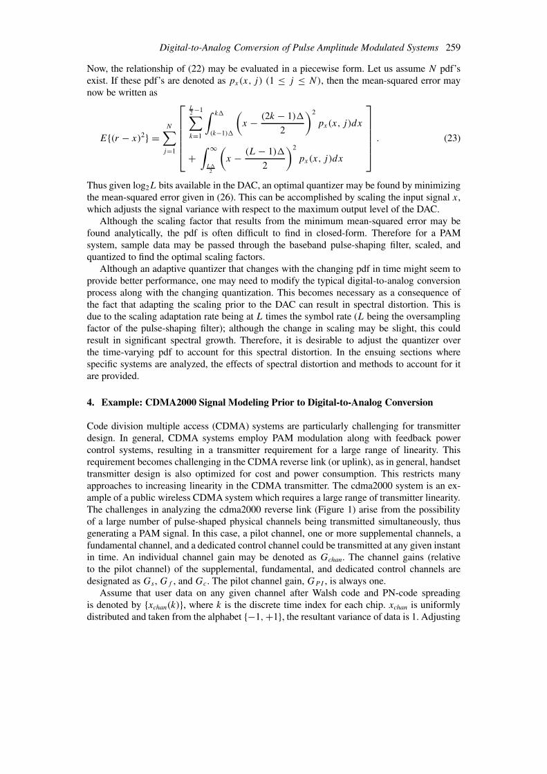
Code division multiple access (CDMA) systems are particularly challenging for transmitterdesign. In general, CDMA systems employ PAM modulation along with feedback powercontrol systems, resulting in a transmitter requirement for a large range of linearity. Thisrequirement becomes challenging in the CDMA reverse link (or uplink), as in general, handsettransmitter design is also optimized for cost and power consumption. This restricts manyapproaches to increasing linearity in the CDMA transmitter. The cdma2000 system is an ex-ample of a public wireless CDMA system which requires a large range of transmitter linearity.The challenges in analyzing the cdma2000 reverse link (Figure 1) arise from the possibilityof a large number of pulse-shaped physical channels being transmitted simultaneously, thusgenerating a PAM signal. In this case, a pilot channel, one or more supplemental channels, afundamental channel, and a dedicated control channel could be transmitted at any given instantin time. An individual channel gain may be denoted as Gchan. The channel gains (relativeto the pilot channel) of the supplemental, fundamental, and dedicated control channels aredesignated as Gs , Gf , and Gc. The pilot channel gain, GPI , is always one.
Assume that user data on any given channel after Walsh code and PN-code spreadingis denoted by {xchan(k)}, where k is the discrete time index for each chip. xchan is uniformlydistributed and taken from the alphabet {−1,+1}, the resultant variance of data is 1. Adjusting
260 Giridhar D. Mandyam
Figure 1. cdma2000 transmitter.
by the channel gain factor results in a variance of G2chan. However, the data is passed through
a baseband pulse-shaping filter. This filter, whose tap spacing is 1/4 of a chip, is 48 taps long.If three zeros are inserted between each datum in {xchan(k)}, then the resultant sequence maybe denoted as {dchan(l)}, where the following applies:
{dchan(l)} = {xchan(0), 0, 0, 0, xchan(1), 0, 0, 0, . . .} . (24)
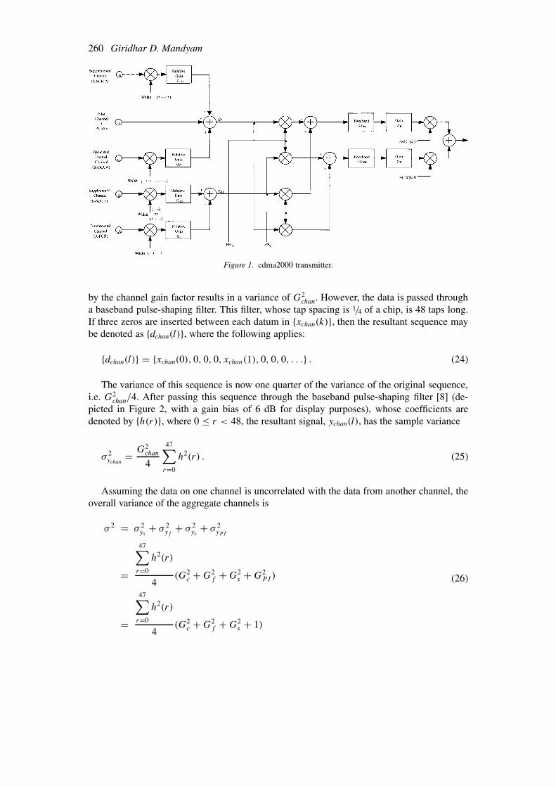
The variance of this sequence is now one quarter of the variance of the original sequence,i.e. G2
chan/4. After passing this sequence through the baseband pulse-shaping filter [8] (de-picted in Figure 2, with a gain bias of 6 dB for display purposes), whose coefficients aredenoted by {h(r)}, where 0 ≤ r < 48, the resultant signal, ychan(l), has the sample variance
σ 2ychan
= G2chan
4
47∑r=0
h2(r) . (25)
Assuming the data on one channel is uncorrelated with the data from another channel, theoverall variance of the aggregate channels is
σ 2 = σ 2ys
+ σ 2yf
+ σ 2ys
+ σ 2yPI
=
47∑r=0
h2(r)
4(G2
c + G2f + G2
s + G2PI )
=
47∑r=0
h2(r)
4(G2
c + G2f + G2
s + 1)
(26)
Digital-to-Analog Conversion of Pulse Amplitude Modulated Systems 261
Figure 2. cdma2000 baseband filter.
262 Giridhar D. Mandyam
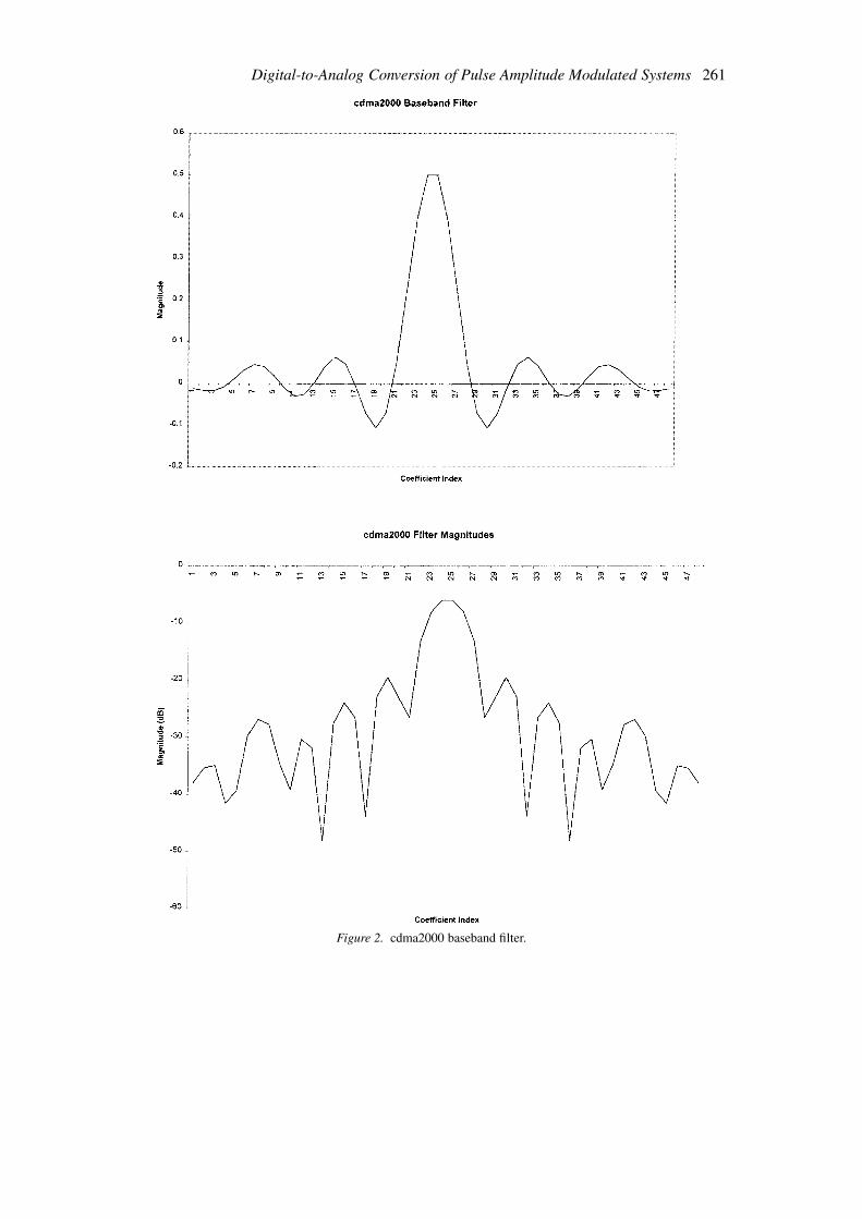
Figure 3. First 12-tuple of coefficients, h1(r).
ychan(l) is not Gaussian. This can be seen by referring to the convolution relationship thatdefines ychan(l):
ychan(l) =47∑i=0
h(i)dchan(l − i) . (27)
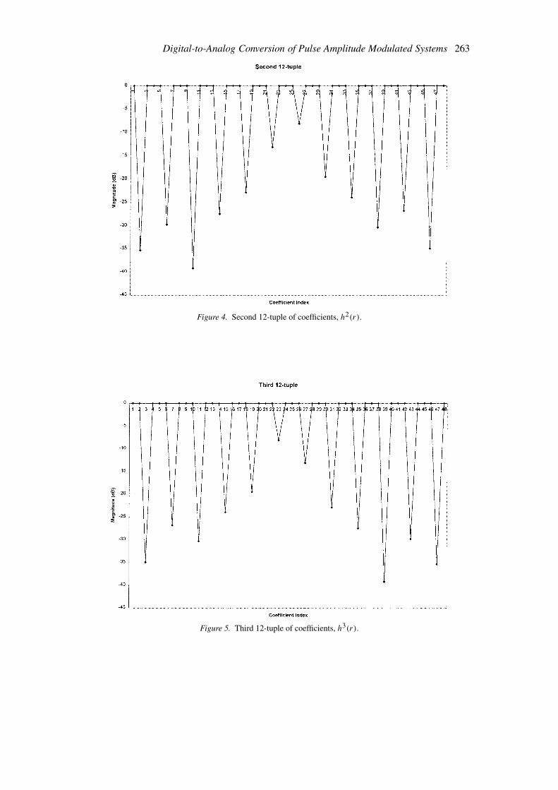
Although the convolution equation indicates that the calculation of ychan(l) results from 48multiplications and 47 additions; in fact, due to the zero insertion in dchan(l), the result actuallycomes about from 12 multiplications and 11 additions. Assuming that the filter coefficientsmay be represented by the corresponding 12-tuples, i.e. {h(r)} = {h1(r), h2(r), h3(r), h4(r)},where hi(r) is a group of 12 filter coefficients resulting in a single filter output, then byobserving the gains resulting from multiplication from each group of 12 coefficients fromh(r) (Figures 3–6), one can see that in two cases only one of the coefficients is dominant.Thus central limit theorem arguments for Gaussianity become ineffective.
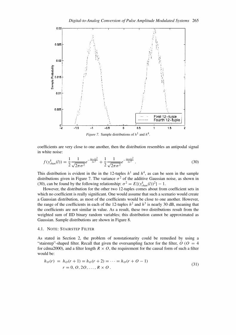
A typical distribution of coefficients for one channel output based on the 12-tuple of Fig-ure 3 is shown in Figure 7. As expected, since the convolution sum is basically dominatedby one filter coefficient, the distribution resembles that of an antipodal signal in white noise.The “white noise” in this case is a result of the contributions of the smaller filter coefficients(“smaller” in this case means any coefficients other than the maximum gain coefficient ineach 12-tuple of filter coefficients). As there is more than one smaller coefficient of similargain value in this particular 12-tuple of filter coefficients, the central limit theorem argumentis strengthened for the filter output due to one 12-tuple alone. This topic will be examined inmore detail.
Due to the fact that the “dominant” coefficient changes in magnitude between each of the12-tuples, the process resulting from the baseband filter is in fact cyclostationary. This can be
Digital-to-Analog Conversion of Pulse Amplitude Modulated Systems 263
Figure 4. Second 12-tuple of coefficients, h2(r).
Figure 5. Third 12-tuple of coefficients, h3(r).
264 Giridhar D. Mandyam
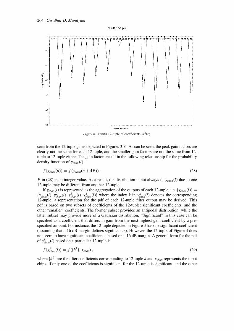
Figure 6. Fourth 12-tuple of coefficients, h4(r).
seen from the 12-tuple gains depicted in Figures 3–6. As can be seen, the peak gain factors areclearly not the same for each 12-tuple, and the smaller gain factors are not the same from 12-tuple to 12-tuple either. The gain factors result in the following relationship for the probabilitydensity function of ychan(l):
f (ychan(n)) = f (ychan(n + 4P)) . (28)
P in (28) is an integer value. As a result, the distribution is not always of ychan(l) due to one12-tuple may be different from another 12-tuple.
If ychan(l) is represented as the aggregation of the outputs of each 12-tuple, i.e. {ychan(l)} ={y1
chan(l), y2chan(l), y
3chan(l), y
4chan(l)} where the index k in yk
chan(l) denotes the corresponding12-tuple, a representation for the pdf of each 12-tuple filter output may be derived. Thispdf is based on two subsets of coefficients of the 12-tuple: significant coefficients, and theother “smaller” coefficients. The former subset provides an antipodal distribution, while thelatter subset may provide more of a Gaussian distribution. “Significant” in this case can bespecified as a coefficient that differs in gain from the next highest gain coefficient by a pre-specified amount. For instance, the 12-tuple depicted in Figure 3 has one significant coefficient(assuming that a 16 dB margin defines significance). However, the 12-tuple of Figure 4 doesnot seem to have significant coefficients, based on a 16 dB margin. A general form for the pdfof yk
chan(l) based on a particular 12-tuple is
f (ykchan(l)) = f ({hk}, xchan) , (29)
where {hk} are the filter coefficients corresponding to 12-tuple k and xchan represents the inputchips. If only one of the coefficients is significant for the 12-tuple is significant, and the other
Digital-to-Analog Conversion of Pulse Amplitude Modulated Systems 265
Figure 7. Sample distributions of h1 and h4.
coefficients are very close to one another, then the distribution resembles an antipodal signalin white noise:
f (ykchan(l)) = 1
2
1√2πσ 2
e− (x−1)2
2σ2 + 1
2
1√2πσ 2
e− (x+1)2
2σ2 . (30)
This distribution is evident in the in the 12-tuples h1 and h4, as can be seen in the sampledistributions given in Figure 7. The variance σ 2 of the additive Gaussian noise, as shown in(30), can be found by the following relationship: σ 2 = E{(yk
chan(l))2} − 1.
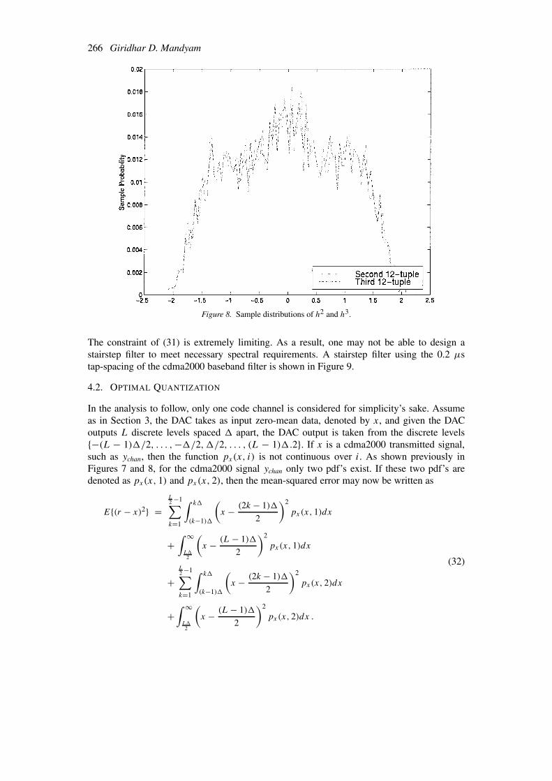
However, the distribution for the other two 12-tuples comes about from coefficient sets inwhich no coefficient is really significant. One would assume that such a scenario would createa Gaussian distribution, as most of the coefficients would be close to one another. However,the range of the coefficients in each of the 12-tuples h2 and h3 is nearly 30 dB, meaning thatthe coefficients are not similar in value. As a result, these two distributions result from theweighted sum of IID binary random variables; this distribution cannot be approximated asGaussian. Sample distributions are shown in Figure 8.
4.1. NOTE: STAIRSTEP FILTER
As stated in Section 2, the problem of nonstationarity could be remedied by using a“stairstep”-shaped filter. Recall that given the oversampling factor for the filter, O (O = 4for cdma2000), and a filter length R × O, the requirement for the causal form of such a filterwould be:
hO(r) = hO(r + 1) = hO(r + 2) = · · · = hO(r + O − 1)
r = 0,O, 2O, . . . , R × O .(31)
266 Giridhar D. Mandyam
Figure 8. Sample distributions of h2 and h3.
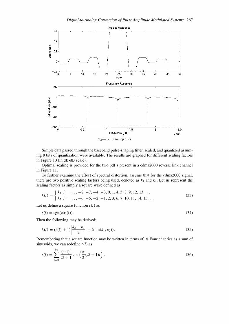
The constraint of (31) is extremely limiting. As a result, one may not be able to design astairstep filter to meet necessary spectral requirements. A stairstep filter using the 0.2 µstap-spacing of the cdma2000 baseband filter is shown in Figure 9.
4.2. OPTIMAL QUANTIZATION
In the analysis to follow, only one code channel is considered for simplicity’s sake. Assumeas in Section 3, the DAC takes as input zero-mean data, denoted by x, and given the DACoutputs L discrete levels spaced � apart, the DAC output is taken from the discrete levels{−(L − 1)�/2, . . . ,−�/2,�/2, . . . , (L − 1)�.2}. If x is a cdma2000 transmitted signal,such as ychan, then the function px(x, i) is not continuous over i. As shown previously inFigures 7 and 8, for the cdma2000 signal ychan only two pdf’s exist. If these two pdf’s aredenoted as px(x, 1) and px(x, 2), then the mean-squared error may now be written as
E{(r − x)2} =L2 −1∑k=1
∫ k�
(k−1)�
(x − (2k − 1)�
2
)2
px(x, 1)dx
+∫ ∞
L�2
(x − (L − 1)�
2
)2
px(x, 1)dx
+L2 −1∑k=1
∫ k�
(k−1)�
(x − (2k − 1)�
2
)2
px(x, 2)dx
+∫ ∞
L�2
(x − (L − 1)�
2
)2
px(x, 2)dx .
(32)
Digital-to-Analog Conversion of Pulse Amplitude Modulated Systems 267
Figure 9. Stairstep filter.
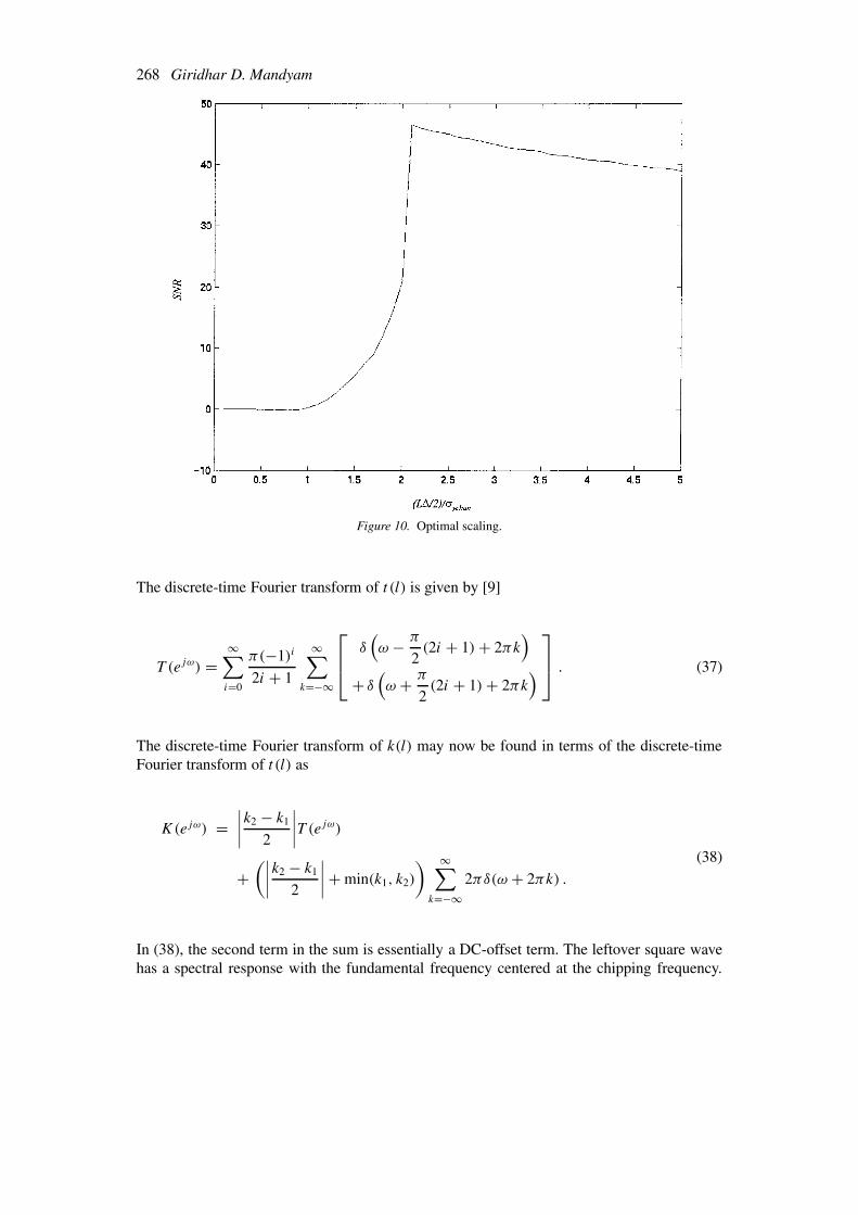
Simple data passed through the baseband pulse-shaping filter, scaled, and quantized assum-ing 8 bits of quantization were available. The results are graphed for different scaling factorsin Figure 10 (in dB-dB scale).
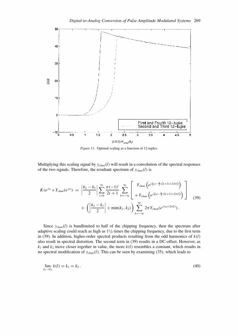
Optimal scaling is provided for the two pdf’s present in a cdma2000 reverse link channelin Figure 11.
To further examine the effect of spectral distortion, assume that for the cdma2000 signal,there are two positive scaling factors being used, denoted as k1 and k2. Let us represent thescaling factors as simply a square wave defined as
k(l) ={k1, l = . . . ,−8,−7,−4,−3, 0, 1, 4, 5, 8, 9, 12, 13, . . .
k2, l = . . . ,−6,−5,−2,−1, 2, 3, 6, 7, 10, 11, 14, 15, . . .(33)
Let us define a square function t (l) as
t (l) = sgn(cos(l)) . (34)
Then the following may be derived:
k(l) = (t (l) + 1)
∣∣∣∣k2 − k1
2
∣∣∣∣ + (min(k1, k2)). (35)
Remembering that a square function may be written in terms of its Fourier series as a sum ofsinusoids, we can redefine t (l) as
t (l) =∞∑i=0
(−1)i
2i + 1cos
(π
2(2i + 1)l
). (36)
268 Giridhar D. Mandyam
Figure 10. Optimal scaling.
The discrete-time Fourier transform of t (l) is given by [9]
T (ejω) =∞∑i=0
π(−1)i
2i + 1
∞∑k=−∞
δ
(ω − π
2(2i + 1) + 2πk
)+ δ
(ω + π
2(2i + 1) + 2πk
) . (37)
The discrete-time Fourier transform of k(l) may now be found in terms of the discrete-timeFourier transform of t (l) as
K(ejω) =∣∣∣∣k2 − k1
2
∣∣∣∣T (ejω)
+(∣∣∣∣k2 − k1
2
∣∣∣∣ + min(k1, k2)
) ∞∑k=−∞
2πδ(ω + 2πk) .
(38)
In (38), the second term in the sum is essentially a DC-offset term. The leftover square wavehas a spectral response with the fundamental frequency centered at the chipping frequency.
Digital-to-Analog Conversion of Pulse Amplitude Modulated Systems 269
Figure 11. Optimal scaling as a function of 12-tuples.
Multiplying this scaling signal by ychan(l) will result in a convolution of the spectral responsesof the two signals. Therefore, the resultant spectrum of ychan(l) is
K(ejω ∗ Ychan(ejω) =
∣∣∣∣k2 − k1
2
∣∣∣∣∞∑i=0
π(−1)i
2i + 1
∞∑k=−∞
Ychan
(ej(ω− π
2 (2i+1)+2πk))
+Ychan
(ej(ω− π
2 (2i+1)+2πk))
+(∣∣∣∣k2 − k1
2
∣∣∣∣ + min(k1, k2)
) ∞∑k=−∞
2πYchan(ej (ω+2πk)) .
(39)
Since ychan(l) is bandlimited to half of the chipping frequency, then the spectrum afteradaptive scaling could reach as high as 11/2 times the chipping frequency, due to the first termin (39). In addition, higher-order spectral products resulting from the odd harmonics of k(l)
also result in spectral distortion. The second term in (39) results in a DC-offset. However, ask1 and k2 move closer together in value, the more k(l) resembles a constant, which results inno spectral modification of ychan(l). This can be seen by examining (35), which leads to
limk1→k2
k(l) = k1 = k2 . (40)

270 Giridhar D. Mandyam
As a result, the following spectrum results
limk1→k2
K(ejω) ∗ Ychan(ejω) = k1
∞∑k=−∞
2πYchan(ej (ω+2πk))
= k2
∞∑k=−∞
2πYchan(ej (ω+2πk)) .
(41)
Thus, if the optimal scaling factor is different for the different distributions, an adaptivequantization algorithm may result in significant spectral growth; there exists a tradeoff be-tween spectral growth and quantization noise. One may try and “undo” the adaptive scaling atthe output of the D/A converter (which results in an inversion of k(l)), but this would requirerapidly switching amplification in the analog domain, which adds a degree of complexity totransceiver design.
“Undoing” the spectral distortion after D/A conversion involves rescaling the data. Thisinvolves simply multiplying the converted signal by 1/k(l). Additional amplification may beneeded if the rescaling operation results in a deviation from the desired output power.
The quantization noise may be derived from either Figure 10 or Figure 11, dependingon the type of quantization scheme used. It should be noted that all previous quantizationanalysis was performed with respect to one channel; if the signal results from aggregating andscaling channels, then this quantization analysis is not optimal. However, based on a fixed-gainscenario, an optimal quantization characteristic may be found.
4.3. CHANNEL AGGREGATION
In the case of channel aggregation, the optimal quantizers derived above will change. This isdue to the fact that the distributions of the data after channel aggregation, although cyclosta-tionary, will vary with the number of channels and the channel scaling. However, one may usethe exact same methodology for deriving a fixed-scaling or adaptive-scaling quantizer, givena scenario for channel aggregation.
The modulation for the reverse link of cdma2000, as pictured in Figure 1, will still resultin 4 distinct distributions from each baseband filter on I and on Q.
5. Example: IS-136 Signal Modeling Prior to Digital-to-Analog Conversion
The IS-136 TDMA system is widely deployed in North America and must meet electro-magnetic compatibility constraints with a wide variety of consumer electronics equipment.Therefore, similar to cdma2000, design constraints exist for IS-136 in terms of emissions.The IS-136 system, being a pulse-shaped system, is sensitive to the restricted dynamic rangeof typical transceivers.
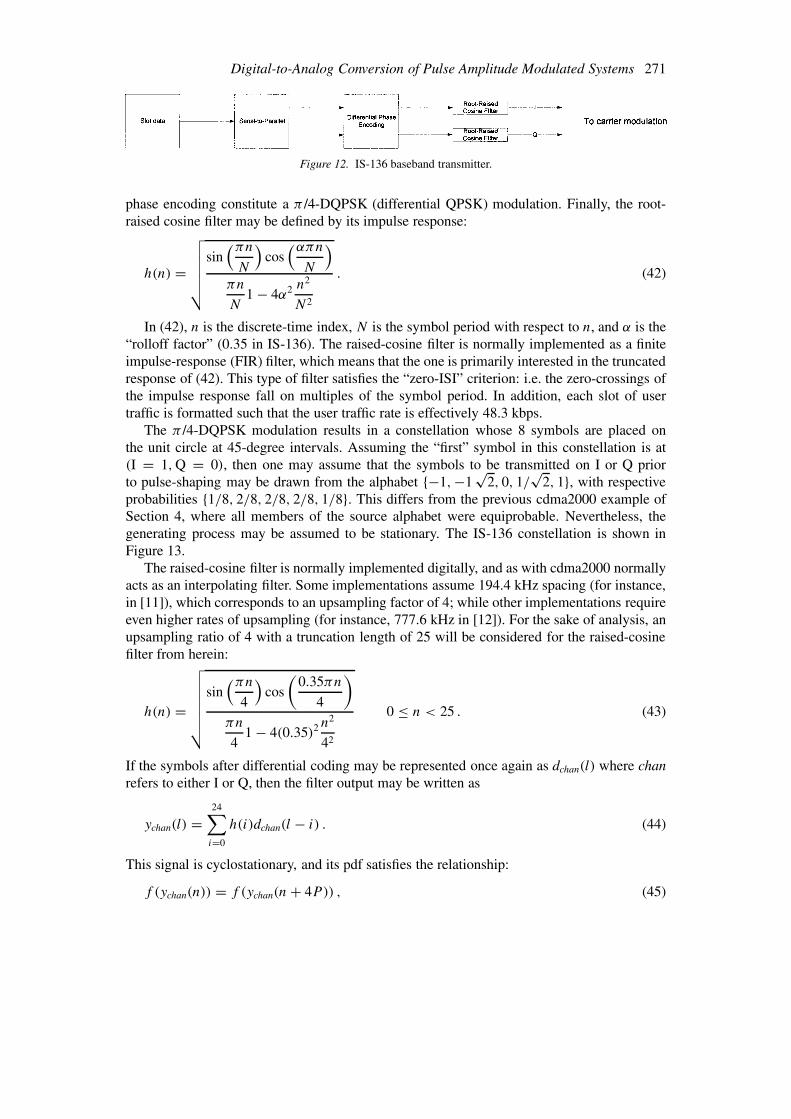
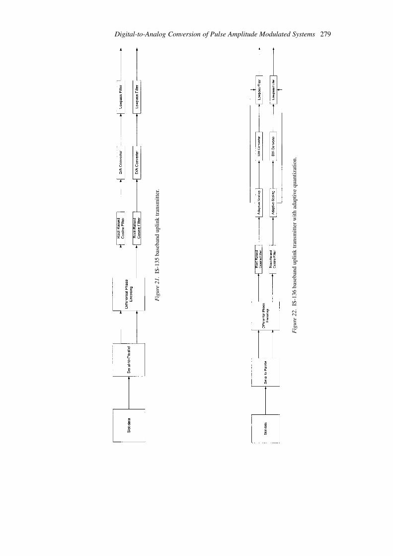
Of primary interest is the IS-136 uplink transmitter. A typical transmitter is shown inFigure 12 [10].
In Figure 12, the slot data is the user traffic for its time slot (there are 6 slots per 40 msperiod). In addition, the combination of the serial-to-parallel converter and the differential
Digital-to-Analog Conversion of Pulse Amplitude Modulated Systems 271
Figure 12. IS-136 baseband transmitter.
phase encoding constitute a π /4-DQPSK (differential QPSK) modulation. Finally, the root-raised cosine filter may be defined by its impulse response:
h(n) =
√√√√√√sin
(πn
N
)cos
(απn
N
)πn
N1 − 4α2 n2
N2
. (42)
In (42), n is the discrete-time index, N is the symbol period with respect to n, and α is the“rolloff factor” (0.35 in IS-136). The raised-cosine filter is normally implemented as a finiteimpulse-response (FIR) filter, which means that the one is primarily interested in the truncatedresponse of (42). This type of filter satisfies the “zero-ISI” criterion: i.e. the zero-crossings ofthe impulse response fall on multiples of the symbol period. In addition, each slot of usertraffic is formatted such that the user traffic rate is effectively 48.3 kbps.
The π /4-DQPSK modulation results in a constellation whose 8 symbols are placed onthe unit circle at 45-degree intervals. Assuming the “first” symbol in this constellation is at(I = 1,Q = 0), then one may assume that the symbols to be transmitted on I or Q priorto pulse-shaping may be drawn from the alphabet {−1,−1
√2, 0, 1/
√2, 1}, with respective
probabilities {1/8, 2/8, 2/8, 2/8, 1/8}. This differs from the previous cdma2000 example ofSection 4, where all members of the source alphabet were equiprobable. Nevertheless, thegenerating process may be assumed to be stationary. The IS-136 constellation is shown inFigure 13.
The raised-cosine filter is normally implemented digitally, and as with cdma2000 normallyacts as an interpolating filter. Some implementations assume 194.4 kHz spacing (for instance,in [11]), which corresponds to an upsampling factor of 4; while other implementations requireeven higher rates of upsampling (for instance, 777.6 kHz in [12]). For the sake of analysis, anupsampling ratio of 4 with a truncation length of 25 will be considered for the raised-cosinefilter from herein:
h(n) =
√√√√√√√sin
(πn
4
)cos
(0.35πn
4
)πn
41 − 4(0.35)2 n
2
42
0 ≤ n < 25 . (43)
If the symbols after differential coding may be represented once again as dchan(l) where chanrefers to either I or Q, then the filter output may be written as
ychan(l) =24∑i=0
h(i)dchan(l − i) . (44)
This signal is cyclostationary, and its pdf satisfies the relationship:
f (ychan(n)) = f (ychan(n + 4P)) , (45)
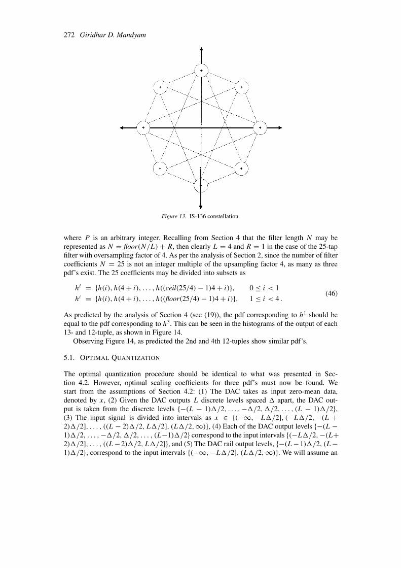
272 Giridhar D. Mandyam
Figure 13. IS-136 constellation.
where P is an arbitrary integer. Recalling from Section 4 that the filter length N may berepresented as N = floor(N/L) + R, then clearly L = 4 and R = 1 in the case of the 25-tapfilter with oversampling factor of 4. As per the analysis of Section 2, since the number of filtercoefficients N = 25 is not an integer multiple of the upsampling factor 4, as many as threepdf’s exist. The 25 coefficients may be divided into subsets as
hi = {h(i), h(4 + i), . . . , h((ceil(25/4) − 1)4 + i)}, 0 ≤ i < 1
hi = {h(i), h(4 + i), . . . , h((floor(25/4) − 1)4 + i)}, 1 ≤ i < 4 .(46)
As predicted by the analysis of Section 4 (see (19)), the pdf corresponding to h1 should beequal to the pdf corresponding to h3. This can be seen in the histograms of the output of each13- and 12-tuple, as shown in Figure 14.
Observing Figure 14, as predicted the 2nd and 4th 12-tuples show similar pdf’s.
5.1. OPTIMAL QUANTIZATION
The optimal quantization procedure should be identical to what was presented in Sec-tion 4.2. However, optimal scaling coefficients for three pdf’s must now be found. Westart from the assumptions of Section 4.2: (1) The DAC takes as input zero-mean data,denoted by x, (2) Given the DAC outputs L discrete levels spaced � apart, the DAC out-put is taken from the discrete levels {−(L − 1)�/2, . . . ,−�/2,�/2, . . . , (L − 1)�/2},(3) The input signal is divided into intervals as x ∈ {(−∞,−L�/2], (−L�/2,−(L +2)�/2], . . . , ((L − 2)�/2, L�/2], (L�/2,∞)}, (4) Each of the DAC output levels {−(L −1)�/2, . . . ,−�/2,�/2, . . . , (L−1)�/2} correspond to the input intervals {(−L�/2,−(L+2)�/2], . . . , ((L−2)�/2, L�/2]}, and (5) The DAC rail output levels, {−(L−1)�/2, (L−1)�/2}, correspond to the input intervals {(−∞,−L�/2], (L�/2,∞)}. We will assume an

Digital-to-Analog Conversion of Pulse Amplitude Modulated Systems 273
Figure 14. Sample histograms for IS-136 root-raised cosine filter.
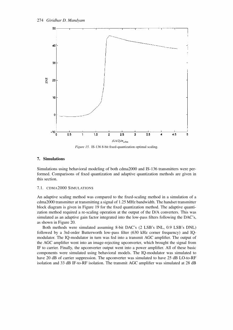
8-bit DAC is being used (as in [12]), and we can derive the optimal fixed quantization scalingby examining the SNR as a function of the scaling coefficient with respect to the input signalvariance, as shown in Figure 15 (dB-dB scale).
The scaling as a function of n-tuple pdf’s is shown in Figure 16 (dB-dB scale).The peak SNR for the fixed quantization (optimized over the entire pdf of the signal) is
45.9 dB, while the mean peak SNR for the adaptive quantization method (optimized for theinstantaneous pdf) is 46.24 dB.
For comparison, similar analysis (not pictured) for 10-bit quantization methods shows apeak SNR of 57.98 dB for fixed quantization and 58.81 dB for adaptive quantization.
6. Digital-to-Analog Conversion Modeling
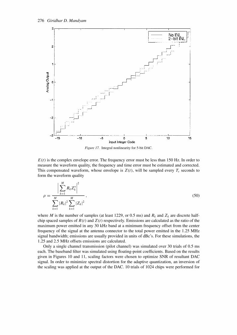
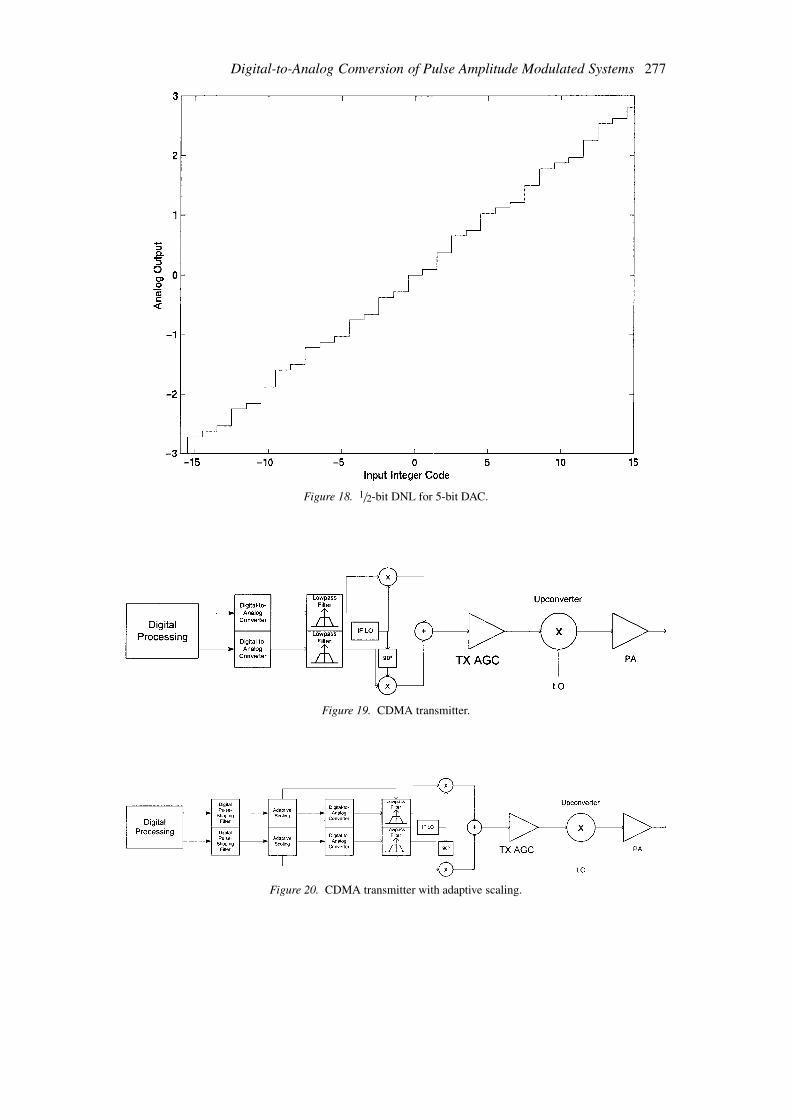
The two main nonidealities that affect D/A converters are integral nonlinearity (INL) anddifferential nonlinearity (DNL). If one thinks of the D/A converter output levels versus thecorresponding input binary codes and then draws a curve through these output levels, then INLdenotes the maximum deviation of this curve from a straight line of unity slope. DNL refersto the maximum deviation of the spacing of the output DAC levels from the ideal spacing ofone least-significant bit (LSB). Both quantities are usually expressed in LSB’s. The conceptof INL is shown in Figure 17.
The deviation from the linear mapping increases quantization noise; however, A/D con-verters may be difficult to design if the INL requirements are very small (much less than 1 bitfor most typical converters). An illustration of quarter-bit DNL is shown in Figure 18.
274 Giridhar D. Mandyam
Figure 15. IS-136 8-bit fixed-quantization optimal scaling.
7. Simulations
Simulations using behavioral modeling of both cdma2000 and IS-136 transmitters were per-formed. Comparisons of fixed quantization and adaptive quantization methods are given inthis section.
7.1. CDMA2000 SIMULATIONS
An adaptive scaling method was compared to the fixed-scaling method in a simulation of acdma2000 transmitter at transmitting a signal of 1.25 MHz bandwidth. The handset transmitterblock diagram is given in Figure 19 for the fixed quantization method. The adaptive quanti-zation method required a re-scaling operation at the output of the D/A converters. This wassimulated as an adaptive gain factor integrated into the low-pass filters following the DAC’s,as shown in Figure 20.
Both methods were simulated assuming 8-bit DAC’s (2 LSB’s INL, 0.9 LSB’s DNL)followed by a 3rd-order Butterworth low-pass filter (630 kHz corner frequency) and IQ-modulator. The IQ-modulator in turn was fed into a transmit AGC amplifier. The output ofthe AGC amplifier went into an image-rejecting upconverter, which brought the signal fromIF to carrier. Finally, the upconverter output went into a power amplifier. All of these basiccomponents were simulated using behavioral models. The IQ-modulator was simulated tohave 20 dB of carrier suppression. The upconverter was simulated to have 25 dB LO-to-RFisolation and 33 dB IF-to-RF isolation. The transmit AGC amplifier was simulated at 28 dB

Digital-to-Analog Conversion of Pulse Amplitude Modulated Systems 275
Figure 16. Adaptive 8-bit scaling.
gain and –15 dBm input IP3. Finally, the PA was simulated to compress at input powers greaterthan 5 dBm, using a typical AM-to-AM and AM-to-PM response to a single-tone [13].
Results were analyzed in terms of emissions and waveform quality [14]. In order to definewaveform quality, one starts out with the ideal transmitted signal. The ideal signal envelope,R(t), is defined as
R(kTs) =∑n
[h(kTs − nTc) cos(φn)]
+ j∑n
[h
(kTs − nTc − Tc
2
)sin(φn)
],
(47)
where Ts is the sampling period, k the sample index, h(t) is the baseband pulse shaping filter,and φn is the phase of the nth chip. Therefore, given the ideal transmitter frequency of ω0, theideal signal at the antenna connector would be
s(t) = R(t)e−jω0t . (48)
The actual transmitted waveform may be written in terms of the ideal signal waveform as
x(t) = C[R(t + τ) + E(t)]e−j (ω0+�ω)(t+τ ) , (49)
where τ is the time offset of the actual signal versus the ideal signal, �ω is the frequencyoffset from the ideal transmitter frequency, and C represents a complex scaling factor, and
276 Giridhar D. Mandyam
Figure 17. Integral nonlinearity for 5-bit DAC.
E(t) is the complex envelope error. The frequency error must be less than 150 Hz. In order tomeasure the waveform quality, the frequency and time error must be estimated and corrected.This compensated waveform, whose envelope is Z(t), will be sampled every Ts seconds toform the waveform quality
ρ =
∣∣∣∣M∑k=1
RkZ∗k
∣∣∣∣2
M∑k=1
|Rk|2M∑k=1
|Zk|2, (50)
where M is the number of samples (at least 1229, or 0.5 ms) and Rk and Zk are discrete half-chip spaced samples of R(t) and Z(t) respectively. Emissions are calculated as the ratio of themaximum power emitted in any 30 kHz band at a minimum frequency offset from the centerfrequency of the signal at the antenna connector to the total power emitted in the 1.25 MHzsignal bandwidth; emissions are usually provided in units of dBc’s. For these simulations, the1.25 and 2.5 MHz offsets emissions are calculated.
Only a single channel transmission (pilot channel) was simulated over 30 trials of 0.5 mseach. The baseband filter was simulated using floating-point coefficients. Based on the resultsgiven in Figures 10 and 11, scaling factors were chosen to optimize SNR of resultant DACsignal. In order to minimize spectral distortion for the adaptive quantization, an inversion ofthe scaling was applied at the output of the DAC. 10 trials of 1024 chips were performed for
Digital-to-Analog Conversion of Pulse Amplitude Modulated Systems 277
Figure 18. 1/2-bit DNL for 5-bit DAC.
Figure 19. CDMA transmitter.
Figure 20. CDMA transmitter with adaptive scaling.

278 Giridhar D. Mandyam
each type of quantization scheme at 6 dB PA backoff. The emissions at 1.25 and 2.5 MHzfor the adaptive quantization algorithm were –58.7 and –76.9 dBc, respectively (the standarddeviations for these two measurements were 1.33 and 6.79 dB, respectively). For the fixedquantization algorithm, the emissions at 1.25 and 2.5 MHz were –57.1 and –70.5 dBc (thestandard deviations were 1.18 and 2.52 dB). The waveform quality for the adaptive quantizerwas 0.9693 (standard deviation 0.0019) and for the fixed quantizer was 0.9698 (standard de-viation 0.0019). The adaptive quantizer provided no performance advantage over the fixedquantizer in terms of waveform quality, but provided smaller emissions. The most likelyreason for improved emissions performance of the adaptive quantizer was due to the reductionin quantization noise, which is usually modeled as wideband.
7.1.1. cdma2000 Simulations: Channel Aggregation CaseIt is of interest to examine the performance of the adaptive scaling method versus the fixedscaling method for the case of channel aggregation. The case which was examined was thecase of pilot and fundamental channel transmission, with the relative channel-to-pilot gain Gf
being 2 (this ratio is robust for a large number cases; for a more rigorous study see [15]). After10 trials of 1024 chips under the same simulation conditions as before, the emissions at 1.25and 2.5 MHz for the adaptive quantization algorithm were –57.0 and –75.4 dBc, respectively(the standard deviations for these two measurements were 1.47 and 3.43 dB, respectively). Forthe fixed quantization algorithm, the emissions at 1.25 and 2.5 MHz were –56.4 and –74.8 dBc(the standard deviations were 1.41 and 3.22 dB). The waveform quality for the adaptive quan-tizer was 0.9659 (standard deviation 0.0013) and for the fixed quantizer was 0.9670 (standarddeviation 0.0014). Once again, the adaptive quantizer provided no performance advantageover the fixed quantizer in terms of waveform quality, but provided smaller emissions.
7.2. IS-136 SIMULATIONS
The IS-136 uplink transmitter was simulated at baseband only. A top-level view of thesimulated transmitter for the fixed quantization method is shown in Figure 21.
The root-raised cosine filter was a 25-tap version truncated version whose tap-spacingwas at 1/4 of the symbol duration. The DAC’s were perfectly linear 8-bit DAC’s, and werefollowed by 4th-order lowpass Butterworth filters whose cutoff was at 70 kHz. The cutofffrequency for the lowpass filters was derived by simulation, and maximized the SNR of thetransmitted signal. Using a simulation bandwidth of 80 times the symbol rate (3.888 MHz),the fixed quantization method was compared to the adaptive quantization method, which wasimplemented as pictured in Figure 22.
The mean SNR after 120 slots of test data for the adaptive quantization method (as mea-sured after the lowpass filter) was 29.9544 dB, while for the same test data set the fixedquantization method yielded 29.6938 dB – a performance difference of 0.26 dB. This is closeto the 0.34 dB performance difference derived from the analysis of Section 5.1.
Digital-to-Analog Conversion of Pulse Amplitude Modulated Systems 279
Fig
ure
21.
IS-1
35ba
seba
ndup
link
tran
smit
ter.
Fig
ure
22.
IS-1
36ba
seba
ndup
link
tran
smit
ter
wit
had
aptiv
equ
anti
zati
on.

280 Giridhar D. Mandyam
8. Conclusions
Fixed and adaptive quantization algorithms were derived with respect to proper scaling andtruncation prior to D/A conversion for pulse amplitude modulated systems. These algo-rithms were simulated using typical parameters for CDMA and transmitters. In particular,the cdma2000 reverse link and IS-136 uplink transmitters were analyzed with respect todigital-to-analog conversion. For the cdma2000 system, simulations demonstrated that theadaptive quantization algorithm provided no performance benefit over the fixed quantizationalgorithm in terms of waveform quality, but provided improvement in terms of emissions. Forthe IS-136 system, simulations showed an enhancement in terms of SNR at baseband afterD/A conversion. This implies that despite the complexity in implementation of an adaptivealgorithm, this approach can be of use when emissions margin is insufficient with the fixedquantization method.
This method of adaptive and/or nonadaptive quantization with respect to the cyclostation-ary pdf of a cdma2000 signal or an IS-136 signal may be extended to any pulse amplitudemodulated system. Further work should examine applications in other communicationssystems that use PAM, regardless of whether such systems are wireless or wireline.
References
1. W.A. Gardner, Cyclostationarity in Communications and Signal Processing, IEEE Press: New York, 1994.2. S. Dennett, The cdma2000 ITU-R RTT Candidate Submission, Ver. 18, The Telecommunications Industry
Association, 1998.3. M. Nettles, M. Chang, G. McAllister, B. Nise, C. Perisco, K. Sahota and J. Tero, “Analog Baseband Processor
for CDMA/FM Portable Cellular Telephones”, in IEEE International Solid-State Circuits Conference 1995,February 1995, pp. 328–329.
4. G. Mandyam, “Analysis of Impact on Handset Transmitter Design of the High-Speed Data Requirements inthe IS-95-B CDMA Wireless Standard”, in IEEE Radio and Wireless Conference, August 1998, pp. 193–196.
5. TIA/EIA-136, The Telecommunications Industry Association, October 16, 1998.6. J. Proakis, Digital Communications, 2nd edn, McGraw-Hill Inc.: New York, 1989.7. N.S. Jayant and P. Noll, Digital Coding of Waveforms: Principles and Applications to Speech and Video,
Prentice-Hall Inc.: Englewood Cliffs, NJ, 1984.8. TIA/EIA/IS-95-A: Mobile Station-Base Station Compatibility Standard for Dual-Mode Wideband Spread
Spectrum Cellular System, The Telecommunications Industry Association, 1995.9. A.V. Oppenheim and R.W. Schafer, Discrete-Time Signal Processing, Prentice-Hall Inc.: Englewood Cliffs,
NJ, 1989.10. TIA/EIA-136-131: Digital Traffic Channel Layer 1, The Telecommunications Industry Association, October
16, 1998.11. N. Van Bavel, P.C. Maulik, K.S. Albright and X.-M. Gong, “An Analog/Digital Interface for Cellular
Telephony”, in IEEE 1994 Custom Integrated Conference, May 1-4, 1994, pp. 395–398.12. V. Friedman, K.R. Lakshmikumar, D.L. Price, T.N. Le and J. Kumar, “A Baseband Processor for IS-54
Cellular Telephony”, IEEE Journal of Solid-State Circuits, Vol. 31, No. 5, pp. 646–655, 1996.13. W. Struble, F. McGrath, K. Harrington and P. Nagle, “Understanding Linearity in Wireless Communication
Amplifiers”, IEEE Journal of Solid-State Circuits, Vol. 32, No. 9, pp. 1310–1318, 1997.14. ANSI/J-STD-018: Recommended Minimum Performance Requirements for 1.8 to 2.0 GHz Code Division
Multiple Access (CDMA) Personal Stations, American National Standards Institute, 1996.15. F. Ling, “Pilot Assisted Coherent DS-CDMA Reverse-Link Communications with Optimal Robust Channel
Estimation”, in International Conference on Acoustics, Speech, and Signal Processing 1997, April 21–24,1997, pp. 263–266.

Digital-to-Analog Conversion of Pulse Amplitude Modulated Systems 281
Giridhar D. Mandyam is the research manager of the Wireless Data Access Group at NokiaResearch Center, Irving, Texas. He received the B.S.E.E. degree Magna Cum Laude fromSouthern Methodist Universityn (Dallas, Texas) in 1989, the M.S.E.E. degree from the Uni-versity of Southern California (Los Angeles, California) in 1993, and the Ph.D. degree inelectrical engineering from the University of New Mexico (Albuquerque, New Mexico) in1996. He has worked for several companies on wireless communications equipment, includ-ing Qualcomm and Texas Instruments. In 1998, he joined Nokia, where he has worked onstandardization and implementation concepts for cdma2000, 1X-EV, and WCDMA. He hasauthored or co-authored over 40 journal and conference publications and four book chapters.He also holds four U.S. patents in the area of wireless communications technology.


![Practical loss tangent imaging with amplitude-modulated ...alekslabuda.com/sites/default/files/publications/[2016-03] Practical loss tangent...Practical loss tangent imaging with amplitude-modulated](https://img.dokumen.tips/doc/110x75/5e5c3022c977ff7aba3622fd/practical-loss-tangent-imaging-with-amplitude-modulated-2016-03-practical-loss.jpg)