Embed Size (px)
Citation preview

Digital image processing: What? Why? and How?
Malay K. KunduMachine Intelligence Unit
Indian Statistical Institute, Kolkatawww.isical.ac.in/~malay
9/20/2014 Prof. M. K. Kundu, MIU, ISI 1
9/20/2014 Prof. M. K. Kundu, MIU, ISI 2
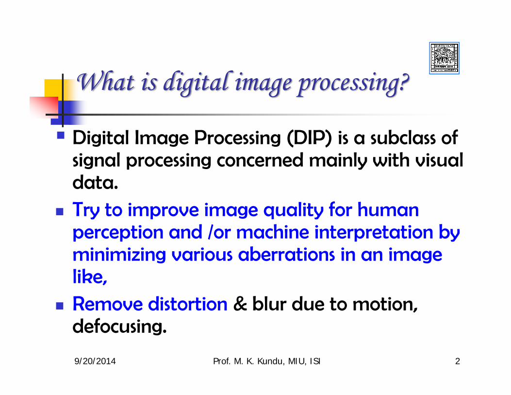
What is digital image processing?
Digital Image Processing (DIP) is a subclass of signal processing concerned mainly with visual data.Try to improve image quality for human perception and /or machine interpretation by minimizing various aberrations in an image like,Remove distortion & blur due to motion, defocusing.

9/20/2014 Prof. M. K. Kundu, MIU, ISI 3
Contd.
Remove roughness, speckles or noise.Improve the contrast and other image qualities.Extract important optical and structural featuresSegment different regions, magnify, rotate etc. Efficiently store the large size image data

9/20/2014 Prof. M. K. Kundu, MIU, ISI 4
Various data processing methods
Input/Output Image Description
Image Digital Image
Processing(DIP)
Computer Vision (CV)
Description Computer Graphics
AI, PR & Data Processing

9/20/2014 Prof. M. K. Kundu, MIU, ISI 5
Major image processing Tasks
Pre-processing (enhancement, smoothing, restoration etc.)
Feature extraction (edge, texture,color, shape and other geometric feature detection.)
Segmentation of different meaningful regions.
Representation and storage/compression of image and video data.

9/20/2014 Prof. M. K. Kundu, MIU, ISI 6
Major application areas of DIP
Document Processing.Remote sensing.Medicine, biology and educational research.Industrial applications.Military applications.Internet and multimedia.Man-machine communication.Forensic and law enforcing.

9/20/2014 Prof. M. K. Kundu, MIU, ISI 7
Example of DIP for various Signal sources
Categorized by image sources : Radiation from Electro-Magnetic(EM) spectrum.Acoustic.Ultrasonic.Electronic (in the form of electronic beams used in electron microscopy).Computer(synthetic images used for modeling and visualization).

9/20/2014 Prof. M. K. Kundu, MIU, ISI 8
Radiation from EM spectrum
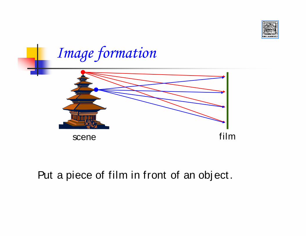
Image formation
scene film
Put a piece of film in front of an object.
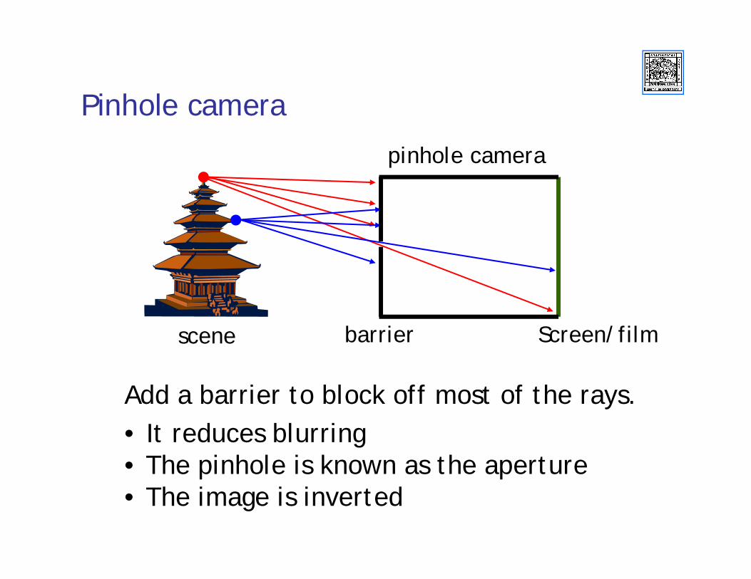
Pinhole camera
scene Screen/film
Add a barrier to block off most of the rays.• It reduces blurring• The pinhole is known as the aperture• The image is inverted
barrier
pinhole camera

Adding a lens
scene screenlens“circle of confusion”
A lens focuses light onto the screen
• There is a specific distance at which objects are “in focus”• other points project to a “circle of confusion” in the image

Lenses
Any object point satisfying this equation is in focus
Thin lens equation:
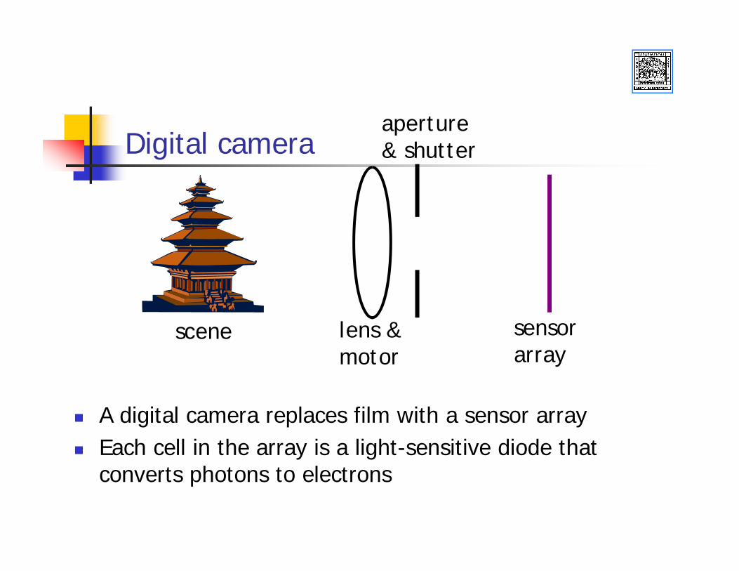
Digital camera
scene sensor array
lens &motor
aperture & shutter
A digital camera replaces film with a sensor arrayEach cell in the array is a light-sensitive diode that converts photons to electrons

Human Eye
9/20/2014 Prof. M. K. Kundu, MIU, ISI 14
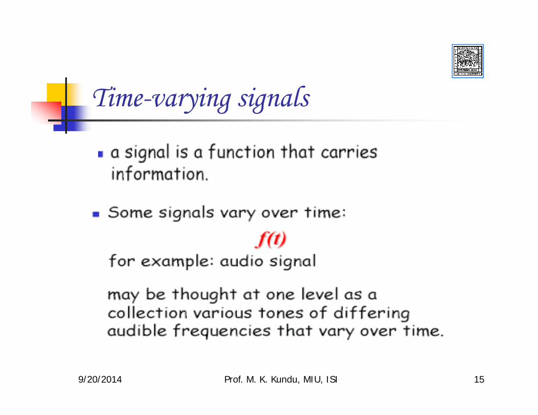
9/20/2014 Prof. M. K. Kundu, MIU, ISI 15
Time-varying signals
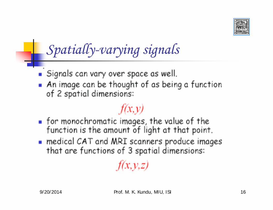
9/20/2014 Prof. M. K. Kundu, MIU, ISI 16
Spatially-varying signals

9/20/2014 Prof. M. K. Kundu, MIU, ISI 17
Analog & Digital signals

9/20/2014 Prof. M. K. Kundu, MIU, ISI 18
Sampling
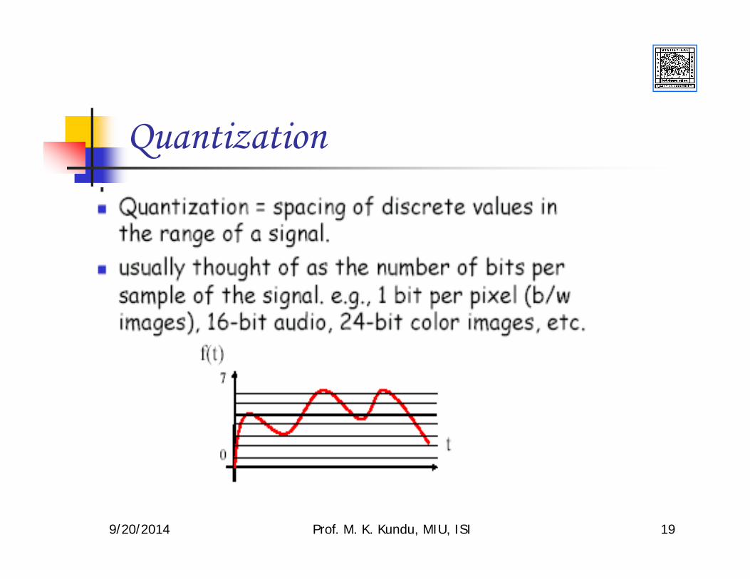
9/20/2014 Prof. M. K. Kundu, MIU, ISI 19
Quantization

9/20/2014 Prof. M. K. Kundu, MIU, ISI 20
Digital Image Representation
9/20/2014 Prof. M. K. Kundu, MIU, ISI 21
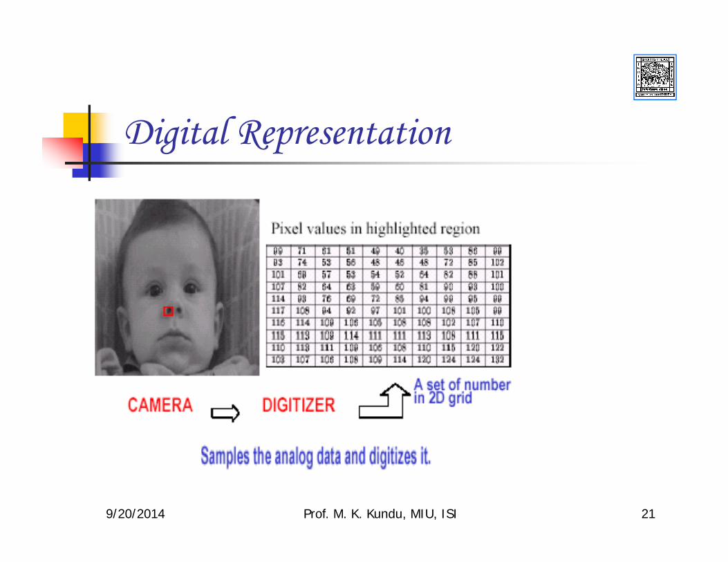
Digital Representation

9/20/2014 Prof. M. K. Kundu, MIU, ISI 22
What is a digital image?
PixelThe picture elements that make up an image, similar to grains in a photograph or dots in a half-tone. Each pixel can represent a number of different shades or colors, depending upon how much storage space is allocated for it.
ResolutionNumber of pixels (in both height and width) making up an image. The higher the resolution of an image, the grater its clarity and definition.

ResolutionThe number of pixels in a given area defines the resolution of an image. A measurement of clarityRefer either to an image file or the device, such as a monitorImage-file resolution is often expressed as a ratio, such as 1000 x 2000Print resolution is expressed in terms of dots per inch(dpi). Image-file resolution and output (print or display) resolution combine to influence the apparent clarity of a digital image when it is viewed.
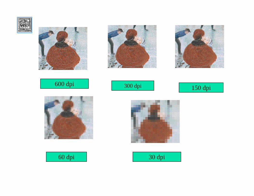
600 dpi 300 dpi 150 dpi
60 dpi 30 dpi
9/20/2014 Prof. M. K. Kundu, MIU, ISI 25
Bit Depth
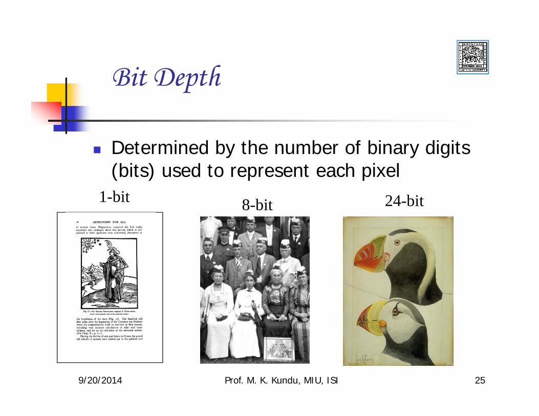
Determined by the number of binary digits (bits) used to represent each pixel
1-bit 8-bit 24-bit
Bit Depth
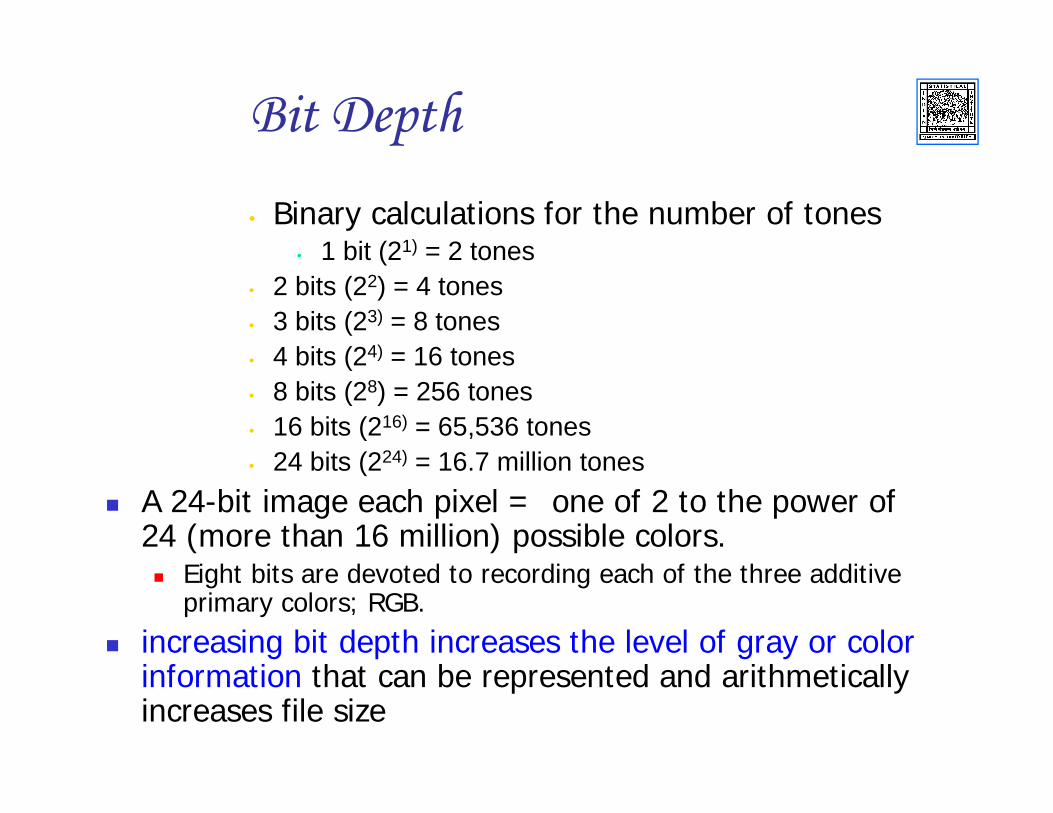
• Binary calculations for the number of tones• 1 bit (21) = 2 tones
• 2 bits (22) = 4 tones• 3 bits (23) = 8 tones• 4 bits (24) = 16 tones• 8 bits (28) = 256 tones• 16 bits (216) = 65,536 tones• 24 bits (224) = 16.7 million tones
A 24-bit image each pixel = one of 2 to the power of 24 (more than 16 million) possible colors.
Eight bits are devoted to recording each of the three additive primary colors; RGB.
increasing bit depth increases the level of gray or color information that can be represented and arithmetically increases file size

Utilizing Sufficient Bit-Depth
3-bit gray 8-bit gray

Utilizing Sufficient Bit Depth
8-bit color 24-bit color

9/20/2014 Prof. M. K. Kundu, MIU, ISI 29
Image Enhancement
What is Image Enhancement?Image enhancement is to process an image so that the result is more suitable than the original image for a Specific application.
Image enhancement is therefore, very much dependent on the particular problem/image at hand.
Image enhancement can be done in either:
Spatial domain: operation on the original image
Frequency domain: operation on the DFT (or other Transform) of the original image
)],([),( nmrTnms =
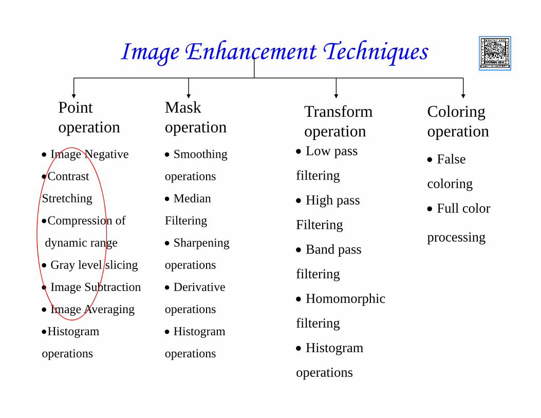
Image Enhancement Techniques
Point operation
Mask operation
Transform operation
Coloring operation
• Image Negative
•Contrast
Stretching
•Compression of
dynamic range
• Gray level slicing
• Image Subtraction
• Image Averaging
•Histogram
operations
• Smoothing
operations
• Median
Filtering
• Sharpening
operations
• Derivative
operations
• Histogram
operations
• Low pass
filtering
• High pass
Filtering
• Band pass
filtering
• Homomorphic
filtering
• Histogram
operations
• False
coloring
• Full color
processing

9/20/2014 Prof. M. K. Kundu, MIU, ISI 32
Objectives of image enhancement
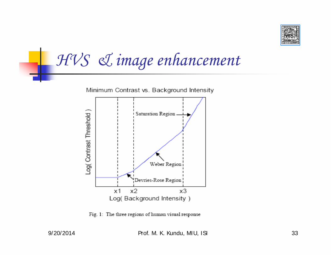
9/20/2014 Prof. M. K. Kundu, MIU, ISI 33
HVS & image enhancement

Histogram Example
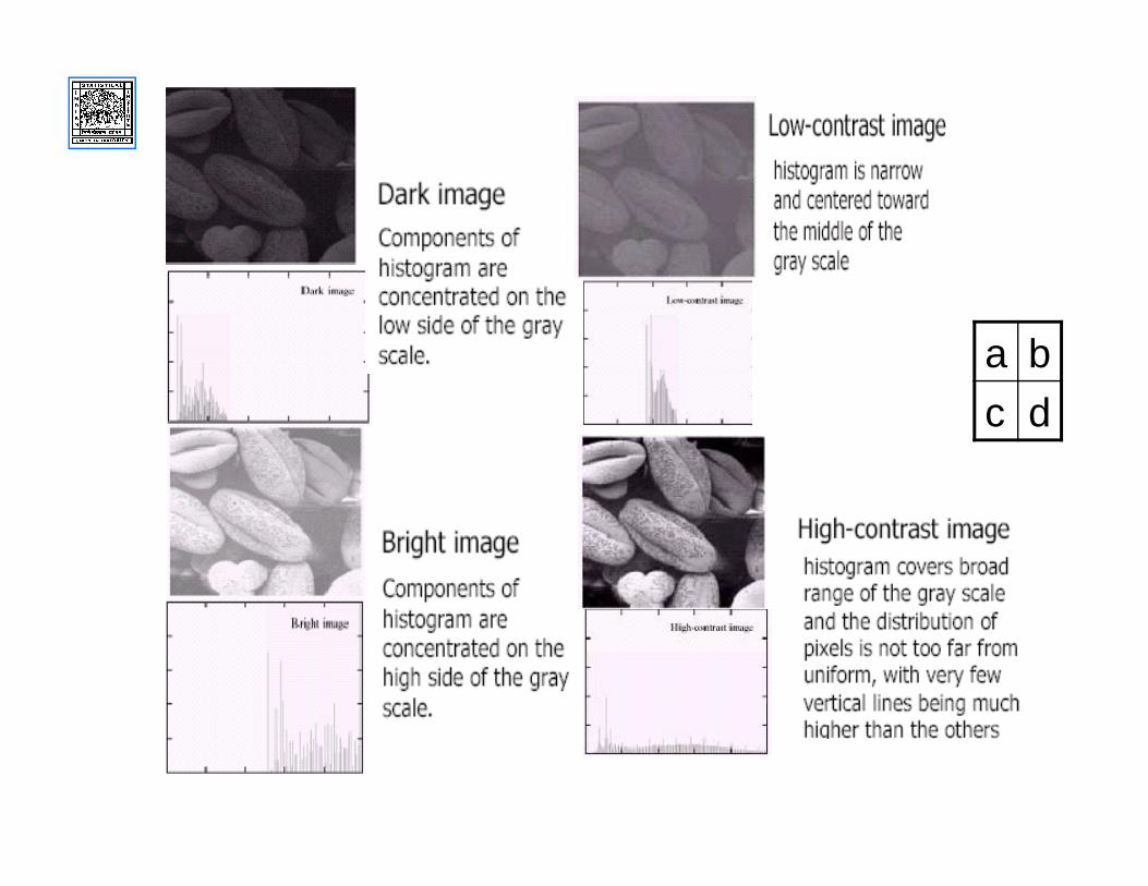
a bc d

Output pixel value s(x,y) at pixel (m,n) depends only on the input pixel value at r(m,n) at (m,n) (and not on the neighboring pixel values).We normally write s=T(r), where s is the output pixel value and r is the input pixel value.
T is any increasing function that maps [0,1] into [0,1].
Point OperationWhat is point operation in image enhancement?

Grey scale remapping is a spatial transformation that only uses a 1x1 neighbourhood around each pixel.
The value at s(x,y) depends directly on the value at r(x,y).

9/20/2014 Prof. M. K. Kundu, MIU, ISI 38
Common gray-level transformation functions
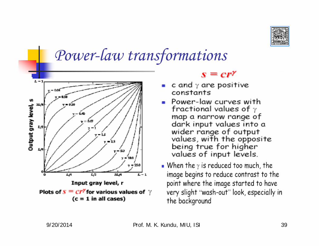
9/20/2014 Prof. M. K. Kundu, MIU, ISI 39
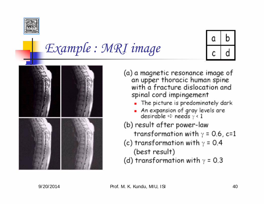
Power-law transformations
9/20/2014 Prof. M. K. Kundu, MIU, ISI 40
Example : MRI image

9/20/2014 Prof. M. K. Kundu, MIU, ISI 41
Example: LFA image

Increase the dynamic range of gray values in the input image.
Suppose you are interested in stretching the input intensity values in the interval [r1 , r2 ]:
Note that (r1 - r2 )<(s1 - s2 ). The gray values in the rang [r1 , r2 ] is stretched into the rang[s1 , s2 ].
Contrast Stretching

Look at the function: 1( )
1 ( / )Es T rm r
= =+
Where r represents the intensities of the input images, s is the corresponding intensity values in the output image, and E controls the slope of the function
That function is called a S-type contrast-stretching transformation. The function compresses the input levels lower than m into a narrow range of dark levels in the output image; similarly, it also compresses the values above m into a narrow band of light levels in the output.

A special case: thresholding or binarization
r1 = r2 =m ; s1 =0 and s2 =1
Useful when we are interested in the shape of the objects.

Example:
Original blood cell binary blood cell

They are obtained by using the transformation function s=T(r). rLrT −−= 1)(
L : maximum gray value
rLrT −−= 1)(
Used mainly in medical images and to produce slides of the screen.
Image Negatives

9/20/2014 Prof. M. K. Kundu, MIU, ISI 47
Negative image
9/20/2014 Prof. M. K. Kundu, MIU, ISI 48
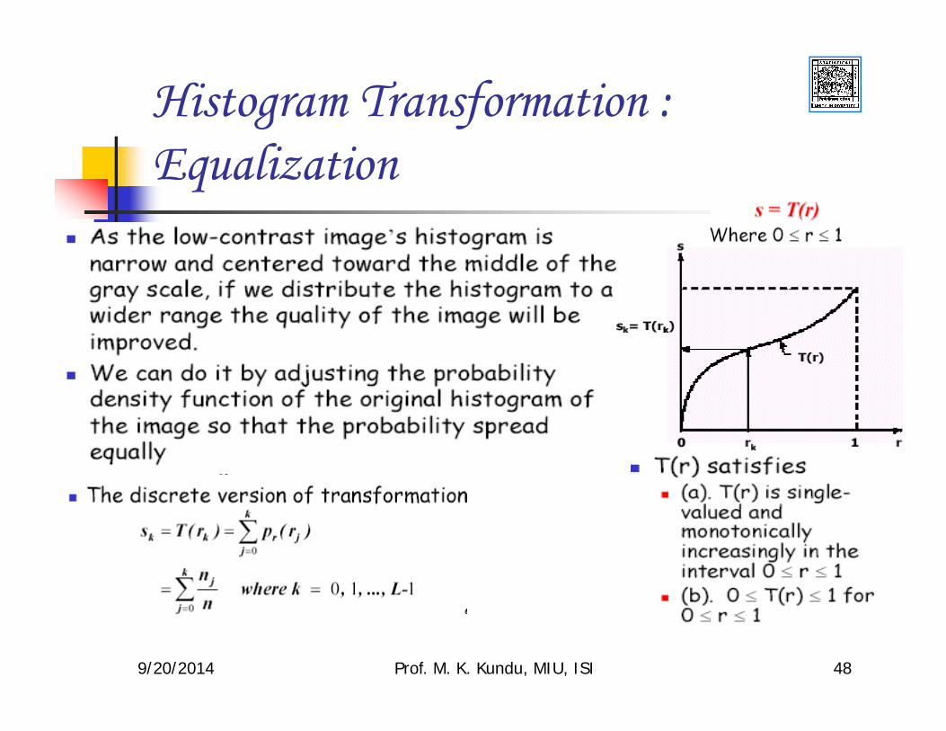
Histogram Transformation : Equalization

Cumulative Histogram
Normal Histogram
Cumulative Histogram

9/20/2014 Prof. M. K. Kundu, MIU, ISI 50
The quality of (d) is not improved much because the original image already has well spread histogram
(a)
(b)
(c)
(d)

Spatial Domain Methods
The value of a pixel at location (x,y) in the enhanced image is the result of performing some operation on the pixels in the neighbourhood of (x,y) in the input image.
Toperator s(x,y)neighbourhood
around r(x,y)
input image f output image g
For computational reasons the neighbourhood is usually square but it can be any shape.

average s(x,y)
input image r output image s
neighbourhoodaround f(x,y)
Spatial Filtering
A common application of spatial filtering is image smoothing using an averaging filter, or averaging mask, or kernel.
Each point in the smoothed image, g(x,y) is obtained from the average pixel value in a neighbourhood of (x,y) in the input image.

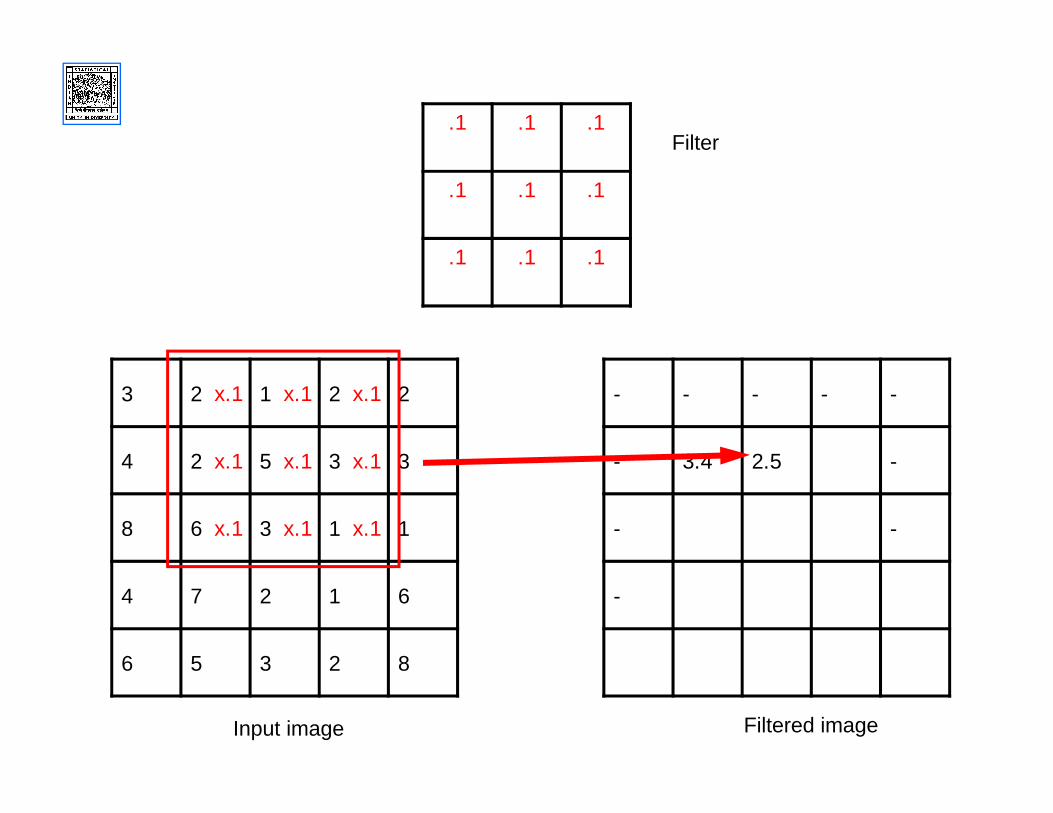
ConvolutionsComputationally, spatial filtering is implemented in a computer program via a mathematical process known as convolution. If we assume a 3x3 neighbourhood the smoothing by averaging would correspond to convolving the image with the following filter, or mask.
This filter is convolved with the image by placing it over a 3x3 portion of the image, multiplying the overlaying pixel values and adding them all up to find the value that replaces the original central pixel value.
1/9 1/9
1/9
1/9
1/9
1/9 1/9
1/9
1/9

3 2 1 2 2
4 2 5 3 3
8 6 3 1 1
4 7 2 1 6
6 5 3 2 8
x.1 x.1 x.1
x.1 x.1 x.1
x.1 x.1 x.1
.1 .1 .1
.1 .1 .1
.1 .1 .1
- - - - -
- 3.4 -
- -
-
Filter
Input image Filtered image
3 2 1 2 2
4 2 5 3 3
8 6 3 1 1
4 7 2 1 6
6 5 3 2 8
x.1 x.1 x.1
x.1 x.1 x.1
x.1 x.1 x.1
.1 .1 .1
.1 .1 .1
.1 .1 .1
- - - - -
- 3.4 2.5 -
- -
-
Filter
Input image Filtered image

3 2 1 2 2
4 2 5 3 3
8 6 3 1 1
4 7 2 1 6
6 5 3 2 8
x.1 x.1 x.1
x.1 x.1 x.1
x.1 x.1 x.1
.1 .1 .1
.1 .1 .1
.1 .1 .1
- - - - -
- 3.4 2.5 2.1 -
- -
-
Filter
Input image Filtered image

3 2 1 2 2
4 2 5 3 3
8 6 3 1 1
4 7 2 1 6
6 5 3 2 8
x.1 x.1 x.1
x.1 x.1 x.1
x.1 x.1 x.1
.1 .1 .1
.1 .1 .1
.1 .1 .1
- - - - -
- 3.4 2.5 2.1 -
- 4.1 -
-
Filter
Input image Filtered image

3 2 1 2 2
4 2 5 3 3
8 6 3 1 1
4 7 2 1 6
6 5 3 2 8
x.1 x.1 x.1
x.1 x.1 x.1
x.1 x.1 x.1
.1 .1 .1
.1 .1 .1
.1 .1 .1
- - - - -
- 3.4 2.5 2.1 -
- 4.1 3.0 -
-
Filter
Input image Filtered image

3 2 1 2 2
4 2 5 3 3
8 6 3 1 1
4 7 2 1 6
6 5 3 2 8
x.1 x.1 x.1
x.1 x.1 x.1
x.1 x.1 x.1
.1 .1 .1
.1 .1 .1
.1 .1 .1
- - - - -
- 3.4 2.5 2.1 -
- 4.1 3.0 2.5 -
-
Filter
Input image Filtered image

3 2 1 2 2
4 2 5 3 3
8 6 3 1 1
4 7 2 1 6
6 5 3 2 8
x.1 x.1 x.1
x.1 x.1 x.1
x.1 x.1 x.1
.1 .1 .1
.1 .1 .1
.1 .1 .1
- - - - -
- 3.4 2.5 2.1 -
- 4.1 3.0 2.5 -
- 4.4
Filter
Input image Filtered image

3 2 1 2 2
4 2 5 3 3
8 6 3 1 1
4 7 2 1 6
6 5 3 2 8
x.1 x.1 x.1
x.1 x.1 x.1
x.1 x.1 x.1
.1 .1 .1
.1 .1 .1
.1 .1 .1
- - - - -
- 3.4 2.5 2.1 -
- 4.1 3.0 2.5 -
- 4.4 3.0
Filter
Input image Filtered image

3 2 1 2 2
4 2 5 3 3
8 6 3 1 1
4 7 2 1 6
6 5 3 2 8
x.1 x.1 x.1
x.1 x.1 x.1
x.1 x.1 x.1
.1 .1 .1
.1 .1 .1
.1 .1 .1
- - - - -
- 3.4 2.5 2.1 -
- 4.1 3.0 2.5 -
- 4.4 3.0 2.7
Filter
Input image Filtered image

3 2 1 2 2
4 2 5 3 3
8 6 3 1 1
4 7 2 1 6
6 5 3 2 8
.1 .1 .1
.1 .1 .1
.1 .1 .1
- - - - -
- 3.4 2.5 2.1 -
- 4.1 3.0 2.5 -
- 4.4 3.0 2.7 -
- - - - -
Filter
Input image Filtered image
The mask is moved across the image until every pixel has been covered.We convolve the image with the mask.

9/20/2014 Prof. M. K. Kundu, MIU, ISI 64
Smoothing

Noise is any random phenomenon that contaminates an image.
Noise is inherent in most practical system:
Image acquisition
Image transmission
Image recordingNoise is typically modeled as an additive process
),(),(),( nmNnmfnmg +=
Noisy image Noise free image
Noise
Image Averaging for Noise Reduction

The noise N(m,n) at each pixel (m,n) is modeled as a random variable.Usually, N(m,n) has Zero-mean and the noise values at different pixels are uncorrelated.
Suppose we have M observations {gi(m,n)}, i=1,2,…,M, we can (partially) mitigate the effect of noise by “averaging”
∑=
=M
ii nmg
Mnmg
1),(1),(
In this case, we can show that
),()],([ nmfnmgE = )],([1)],([ nmNVarM
nmgVar =
Therefore, as the number on observations increases (M infinite), the effect of noise trends to zero.
9/20/2014 Prof. M. K. Kundu, MIU, ISI 67
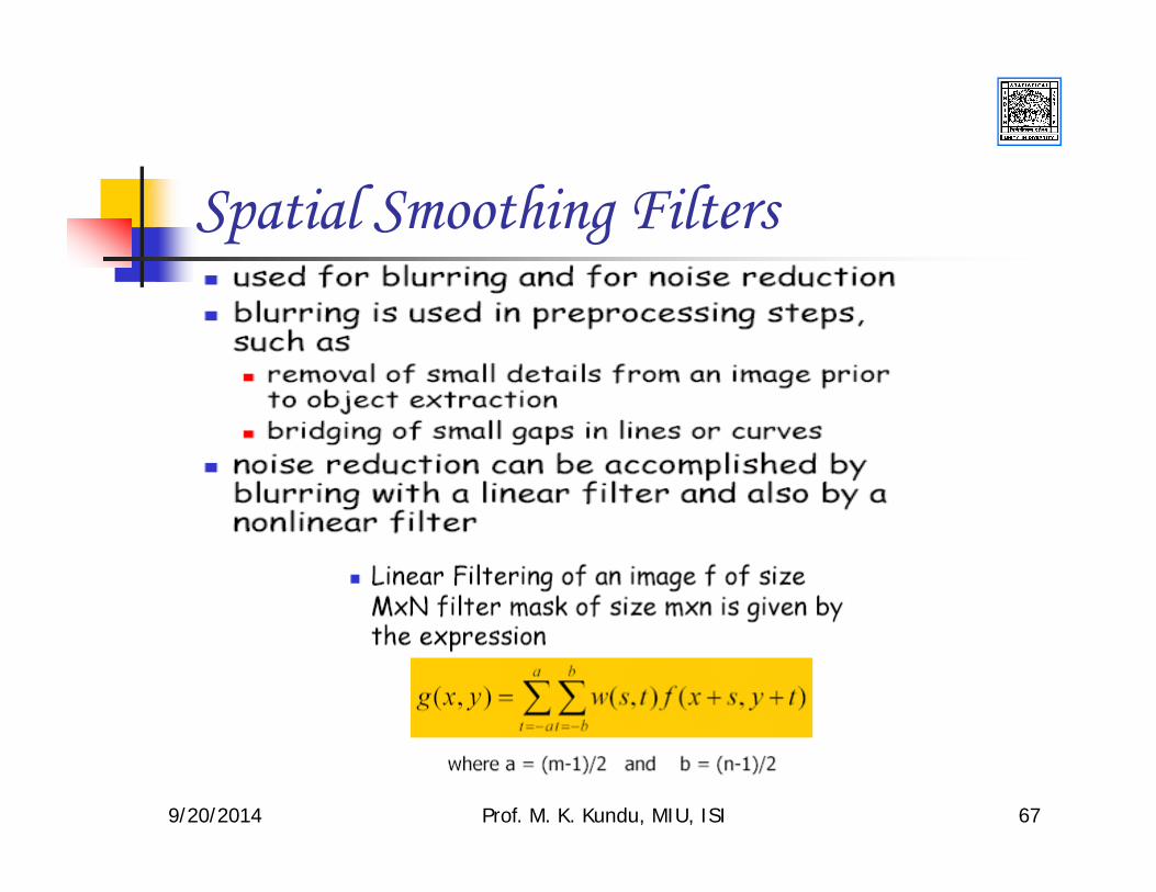
Spatial Smoothing Filters
9/20/2014 Prof. M. K. Kundu, MIU, ISI 68
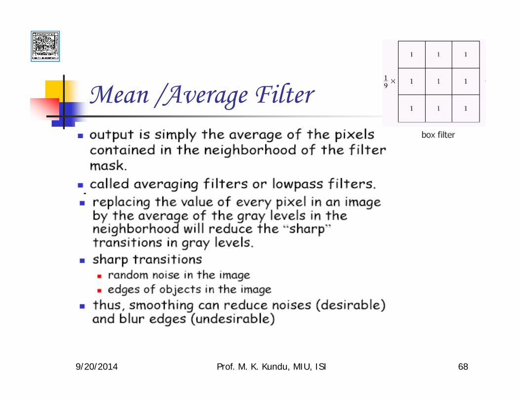
Mean /Average Filter

9/20/2014 Prof. M. K. Kundu, MIU, ISI 69
Weighted average filter

Smoothing is useful when we want to eliminate fine detail, particularly if that detail is an artifact of the image and not part of the inherent information. The larger the smoothing neighborhood, the more blurred the result becomes.

Smoothing can be useful in eliminating "salt and pepper" noise.
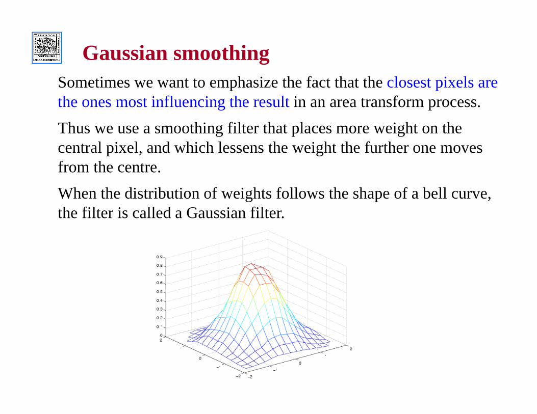
Gaussian smoothingSometimes we want to emphasize the fact that the closest pixels are the ones most influencing the result in an area transform process. Thus we use a smoothing filter that places more weight on the central pixel, and which lessens the weight the further one moves from the centre. When the distribution of weights follows the shape of a bell curve, the filter is called a Gaussian filter.

0.00 0.01 0.02 0.01 0.00 0.01 0.06 0.10 0.06 0.01 0.02 0.10 0.16 0.10 0.02 0.01 0.06 0.10 0.06 0.01 0.00 0.01 0.02 0.01 0.00
A 5x5 mask approximating a Gaussian

9/20/2014 Prof. M. K. Kundu, MIU, ISI 74
Order-statistics (nonlinear) Filters
The other types of filters are mode, k-nearest neighbor, sigma filter etc.
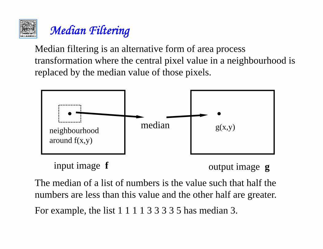
Median FilteringMedian filtering is an alternative form of area process transformation where the central pixel value in a neighbourhood is replaced by the median value of those pixels.
The median of a list of numbers is the value such that half the numbers are less than this value and the other half are greater. For example, the list 1 1 1 1 3 3 3 3 5 has median 3.
median g(x,y)
input image f output image g
neighbourhoodaround f(x,y)

Median filtering is particularly good at removing "salt and pepper" noise whilst preserving edge structure.

9/20/2014 Prof. M. K. Kundu, MIU, ISI 77
Sharpening
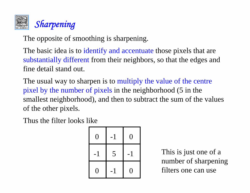
SharpeningThe opposite of smoothing is sharpening. The basic idea is to identify and accentuate those pixels that are substantially different from their neighbors, so that the edges and fine detail stand out. The usual way to sharpen is to multiply the value of the centre pixel by the number of pixels in the neighborhood (5 in the smallest neighborhood), and then to subtract the sum of the values of the other pixels. Thus the filter looks like
5
-1
-1-1
-1 00
00
This is just one of a number of sharpening filters one can use

9/20/2014 Prof. M. K. Kundu, MIU, ISI 79
First and Second order derivative operators.
9/20/2014 Prof. M. K. Kundu, MIU, ISI 80
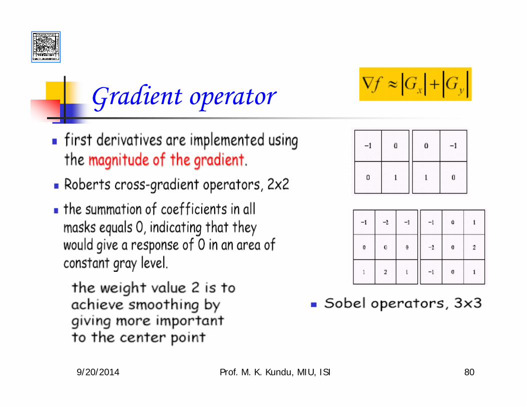
Gradient operator

9/20/2014 Prof. M. K. Kundu, MIU, ISI 81
Laplacian operator & Unsharp Masking
It is a second derivative operator,
High boost filter:

9/20/2014 Prof. M. K. Kundu, MIU, ISI 82
Image SegmentationIt is a comparatively difficult task in image processing.
Aim of this process to separate image objects from the background. Output of this stage is raw pixel data depicting either region boundary or all the points in a region.

9/20/2014 Prof. M. K. Kundu, MIU, ISI 83
Segmentation
Objective of segmentation process is to subdivide an image into its constituent regions or objects. The process stops when all objects of interest in an application are isolated.
Common discontinuities are points, lines and edges

9/20/2014 Prof. M. K. Kundu, MIU, ISI 84
Types of segmentation process
Based on Local features (pixel classification). The important local features used are gray level and its different order of variations, texture, color, surface orientation, flow or motion field etc.Based on global features (Thresholding). The important global features are gray level and different order of variations, color, entropy and other information measures etc.
9/20/2014 Prof. M. K. Kundu, MIU, ISI 85
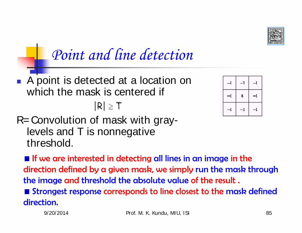
Point and line detectionA point is detected at a location on which the mask is centered if
R=Convolution of mask with gray-levels and T is nonnegative threshold.
If we are interested in detecting all lines in an image in the direction defined by a given mask, we simply run the mask through the image and threshold the absolute value of the result .
Strongest response corresponds to line closest to the mask defined direction.

Origin of Edges
Edges are caused by a variety of factors
depth discontinuity
surface color discontinuity
illumination discontinuity
surface normal discontinuity

9/20/2014 Prof. M. K. Kundu, MIU, ISI 87
Profiles of image intensity edges

9/20/2014 Prof. M. K. Kundu, MIU, ISI 88
Edge detection
1. Detection of short linear edge segments (edgels)
2. Aggregation of edgels into extended edges
3. (maybe parametric description)

Image gradient
The gradient direction is given by:
how does this relate to the direction of the edge? The strength is
The gradient of an image:
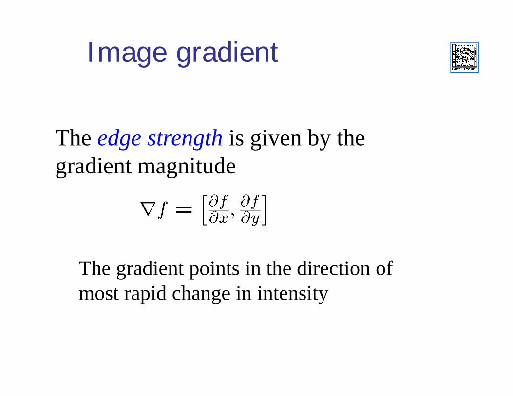
Image gradient
The edge strength is given by the gradient magnitude
The gradient points in the direction of most rapid change in intensity

The discrete gradient
How can we differentiate a digital image f[x,y]?
Option 1: reconstruct a continuous image, then take gradientOption 2: take discrete derivative (finite difference)
How would you implement this as a cross-correlation?

9/20/2014 Prof. M. K. Kundu, MIU, ISI 92
Gradient operators
(a): Roberts’ cross operator (b): 3x3 Prewitt operator(c): Sobel operator (d) 4x4 Prewitt operator

2D edge detection filters
is the Laplacian operator:
Laplacian of Gaussian
Gaussian derivative of Gaussian

9/20/2014 Prof. M. K. Kundu, MIU, ISI 94
Data Compression ?
DATA= Information + Redundancy
Compression is the technique to reduce redundancy in data representation in order to reduce storage requirements and hence communication bandwidth cost.

9/20/2014 Prof. M. K. Kundu, MIU, ISI 95
Classification of Compression
LosslessDecoded data is exact replica of the
original one.Text, Data, Medical Imagery, etc.
9/20/2014 Prof. M. K. Kundu, MIU, ISI 96
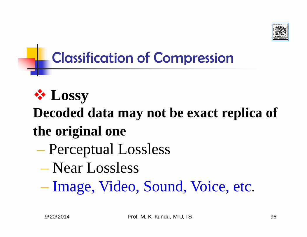
Classification of Compression
Lossy Decoded data may not be exact replica of the original one replica of t– Perceptual Lossless – Near Lossless Loss– Image, Video, Sound, Voice, etc.

9/20/2014 Prof. M. K. Kundu, MIU, ISI 97
File Formats
Consist of both the bits that comprise image information and header information on how to read and interpret the fileImage quality affected by format support for:
Bit depthCompression techniques Color managementHardware,software, and network support
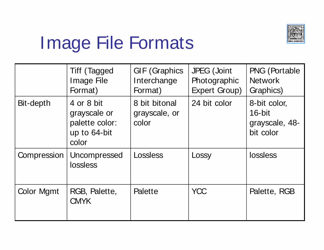
Image File FormatsTiff (Tagged Image File Format)
GIF (Graphics Interchange Format)
JPEG (Joint Photographic Expert Group)
PNG (Portable Network Graphics)
Bit-depth 4 or 8 bit grayscale or palette color: up to 64-bit color
8 bit bitonal grayscale, or color
24 bit color 8-bit color, 16-bit grayscale, 48-bit color
Compression Uncompressed lossless
Lossless Lossy lossless
Color Mgmt RGB, Palette, CMYK
Palette YCC Palette, RGB


Effects of JPEG Compression
300 dpi, 8-bit grayscaleuncompressed TIFF
JPEG 18.5:1 compression

Uncompressed image Lossless compression
Lossy compression
9/20/2014 Prof. M. K. Kundu, MIU, ISI 102
Compression: JPEG
Modes of JPEG (Joint Photographic Expert Group)
Sequential Lossless mode: Decoded image is exact replica of the original decoded image.Sequential DCT based mode: The simplest and widely
used algorithm in this mode is the “Baseline JPEG” Progressive DCT based mode: Encodes image in multiple
scans.Hierarchical Mode: Encodes at multiple resolutions
9/20/2014 Prof. M. K. Kundu, MIU, ISI 103
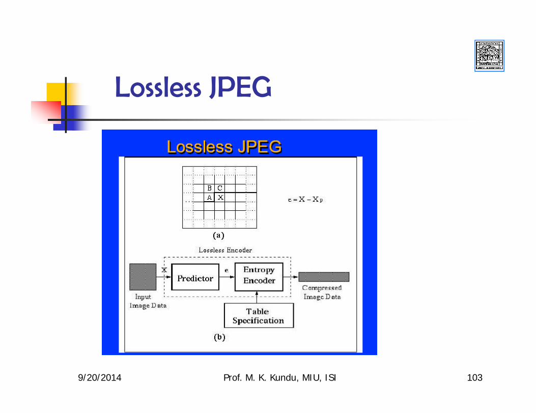
Lossless JPEG

9/20/2014 Prof. M. K. Kundu, MIU, ISI 104
Baseline JPEG Architecture
9/20/2014 Prof. M. K. Kundu, MIU, ISI 105
Reference booksR. C. Gonzalez and R. E. Woods, “Digital Image Processing”, 4th edition, Pearson Education (Singapore) Pte. Ltd, 2011.M. Sonaka, V. Hlavac and R. Boyle, “ Image Processing, Analysis and machine Vision, PWS Publishing, N.Y., 2010. S. K. Pal, A. Ghosh and M. K. Kundu, “ Soft Computing for Image Processing, Physica Verlag, Heidelberg, 2000.D. Salomon “Data Compression,” Springer Verlag, 2002

9/20/2014 Prof. M. K. Kundu, MIU, ISI 106
Thank You


![ECE-V-DIGITAL SIGNAL PROCESSING [10EC52] …vtusolution.in/.../digital-signal-processing-10ec52.pdfDigital vtusolution.in Signal Processing 10EC52 TEXT BOOK: 1. DIGITAL SIGNAL PROCESSING](https://img.dokumen.tips/doc/110x75/5afe42bb7f8b9a256b8ccd2e/ece-v-digital-signal-processing-10ec52-signal-processing-10ec52-text-book.jpg)