Embed Size (px)
Citation preview

4
DIGITAL FILTERS 4.1 Introduction 4.2 Linear Time-Invariant Filters 4.3 Recursive and non-Recursive Filters 7.4 Filtering, Convolution and Correlation Operations 7.5 Filter Structures 4.6 Design of FIR Filters 4.7 Design of Filterbanks 7.8 Design of IIR Filters 7.9 Issues in the Design and Implementation of a Digital Filter
ilters are a basic component of all signal processing and telecommunication systems. The primary functions of a filter are one or more of the followings: (a) to confine a signal into a prescribed frequency
band or channel for example as in anti-aliasing filter or a radio/tv channel selector, (b) to decompose a signal into two or more sub-band signals for sub-band signal processing, for example in music coding, (c) to modify the frequency spectrum of a signal, for example in audio graphic equalizers, and (d) to model the input-output relation of a system such as a mobile communication channel, voice production, musical instruments, telephone line echo, and room acoustics.
In this chapter we introduce the general form of the equation for a linear time-invariant filter and consider the various methods of description of a filter in time and frequency domains. We study different filter forms and structures and the design of low-pass filters, band-pass filters, band-stop filters and filter banks. We consider several applications of filters such as in audio graphic equalizers, noise reduction filters in Dolby systems, image deblurring, and image edge emphasis.
F

2 Chapter 5 Digital Filters
4.1 Introduction Filters are widely employed in signal processing and communication systems in applications such as channel equalization, noise reduction, radar, audio processing, video processing, biomedical signal processing, and analysis of economic and financial data. For example in a radio receiver band-pass filters, or tuners, are used to extract the signals from a radio channel. In an audio graphic equalizer the input signal is filtered into a number of sub-band signals and the gain for each sub-band can be varied manually with a set of controls to change the perceived audio sensation. In a Dolby system pre-filtering and post-filtering are used to minimize the effect of noise. In hi-fi audio a compensating filter may be included in the preamplifier to compensate for the non-ideal frequency-response characteristics of the speakers. Filters are also used to create perceptual audio-visual effects for music, films and in broadcast studios.
The primary functions of filters are one of the followings:
(a) To confine a signal into a prescribed frequency band as in low-pass, high-pass, and band-pass filters.
(b) To decompose a signal into two or more sub-bands as in filter-banks, graphic equalizers, sub-band coders, frequency multiplexers.
(c) To modify the frequency spectrum of a signal as in telephone channel equalization and audio graphic equalizers.
(d) To model the input-output relationship of a system such as telecommunication channels, human vocal tract, and music synthesizers.
Depending on the form of the filter equation and the structure of implementation, filters may be broadly classified into the following classes:
(a) Linear filters versus nonlinear filters.
(b) Time-invariant filters versus time-varying filters.
(c) Adaptive filters versus non-adaptive filters.
(d) Recursive versus non-recursive filters.
(e) Direct-form, cascade-form, parallel-form and lattice structures.
In this chapter we are mainly concerned with linear time-invariant (LTI) filters. These are a class of filters whose output is a linear combination of the input and

Sec. 4.2 Linear Time Invariant Filters 3
whose coefficients do not vary with time. Time-varying and adaptive filters are considered in later chapters.
4.1.1 Alternative Methods for Description of Filters Filters can be described using the following time or frequency domain methods:
(a) Time domain input-output relationship. As described in section 4.2 a difference equation is used to describe the output of a discrete-time filter in terms of a weighted combination of the input and previous output samples. For example a first-order filter may have the following difference equation
)()1()( mxmyamy +−= (4.1)
where x(m) is the filter input, y(m) is the filter output and a is the filter coefficient.
(b) Impulse Response. A filter can be described in terms of its response to an impulse input. For example the response of the filter of Eq. (4.1) to a discrete-time impulse input at m=0 is
mamy =)( m=0, 1, 2, … (4.2)
y(m) = …,,,,,1 432 aaaaa m = for m=0,1,2,3, 4 ... and it is assumed y(-1)=0.
Impulse response is useful because: (i) any signal can be viewed as the sum of a number of shifted and scaled impulses, hence the response a linear filter to a signal is the sum of the responses to all the impulses that constitute the signal, (ii) an impulse input contains all frequencies with equal energy, and hence it excites a filter at all frequencies and (iii) impulse response and frequency response are Fourier transform pairs.
(c) Transfer Function, Poles and Zeros. The transfer function of a digital filter H(z) is the ratio of the z-transforms of the filter output and input given by
)()()(
zXzYzH = (4.3)
For example the transfer function of the filter of Eq. (4.1) is given by
111)(
−−=
zazH (4.4)

4 Chapter 5 Digital Filters
A useful method of gaining insight into the behavior of a filter is the pole-zero description of a filter. As described in Sec. X poles and zeros are the roots of the denominator and numerator of the transfer function respectively.
(d) Frequency Response. The frequency response of a filter describes how the filter alters the magnitude and phase of the input signal frequencies. The frequency response of a filter can be obtained by taking the Fourier transform of the impulse response of the filter, or by simple substitution of the frequency variable ωje for the z variable ωjez = in the z-transfer function as
)()()(
ω
ωω
j
jj
eXeYezH == (4.5)
The frequency response of a filter is a complex variable and can be described in terms of the filter magnitude response and the phase response of the filter.
4.2 Linear Time-Invariant Digital Filters Linear time-invariant (LTI) filters are a class of filters whose output is a linear combination of the input signal samples and whose coefficients do not vary with time. The linear property entails that the filter response to a weighted sum of a number of signals, is the weighted sum of the filter responses to the individual signals. This is the principle of superposition. The term time-invariant implies that the filter coefficients and hence its frequency response is fixed and does not vary with time.
In the time domain the input-output relationship of a discrete-time linear filter is given by the following linear difference equation:
where {ak, bk} are the filter coefficients, and the output y(m) is a linear combination of the previous N output samples [y(m−1),…, y(m−N)], the present input sample x(m) and the previous M input samples [x(m−1),…, x(m−M)]. The characteristic of a filter is completely determined by its coefficients {ak, bk}.
∑∑==
−+−=M
kk
N
kk kmxbkmyamy
01)()()(
(4.6)

Sec. 4.2 Linear Time Invariant Filters 5
For a time-invariant filter the coefficients {ak, bk} are constants calculated to obtain a specified frequency response.
The filter transfer function, obtained by taking the z-transform of the difference equation (4.6), is given by:
The frequency response of this filter can be obtained from Eq. (4.7) by substituting the frequency variable ωje for the z variable, ω= jez , as
∑
∑
=
−
=
−
−
=N
k
kk
M
k
kk
ea
ebeH
1
j
0
j
j
1)(
ω
ω
ω (4.8)
Since from Fourier transform a signal is a weighted combination of a number of sine waves, it follows, from superposition principle, that in frequency domain linear filtering can be viewed as linear combination of the frequency constituents of the input multiplied by the frequency response of the signal.
Filter Order – The order of a discrete-time filter is the highest discrete-time delay used in the input-output equation of the filter. For Example, in Equations (4.6 or 4.7) the filter order is the larger of the values of N or M. For continuous-time filters the filter order is the order of the highest differential term used in the input-output equation of the filter.
4.3 Recursive and non-Recursive Filters Fig. 4.1 shows a block diagram implementation of the linear time-invariant filter Eq. (4.1). The transfer function of the filter in Eq. (4.7) is the ratio of two polynomials in the variable z and may be written in a cascade form as
)()()( 21 zHzHzH = (4.9)
∑
∑
=
−
=
−
−
= N
k
kk
M
k
kk
za
zbzH
1
0
1)( (4.7)

6 Chapter 5 Digital Filters
where H1(z) is the transfer function of a feed-forward, all-zero, filter given by
∑=
−=M
k
kk zbzH
01 )( (4.10)
and H2(z) is the transfer function of a feedback, all-pole, recursive filter given by
∑=
−−
=N
k
kk za
zH
1
2
1
1)( (4.11)
z – 1
x(m)b0
b1
a2
z –1
a1
b2
z –1
z –1
z –1
bM–1
aN
aN – 1
bM
z – 1
y(m)
......
∑=
−M
kk kmxb
0
)( ∑=
−N
kk kmya
1
)(
Non-recursiveall-zero part
Recursive all-pole part
Figure 4.1 Illustration of a direct-form pole-zero IIR filter showing the output is composed of the sum of two vector products: a weighted combination of the input samples [b0, …, bM][x(m), …, x(M-1)]T plus a weighted combination of the output feedback [a1, …, aN][y(m-1), …, y(m-N)]T. T denotes transpose.

Sec. 4.3 Recursive and non Recursive Filters 7
z –1z –1 z –1
. . .
b1 b2 bM–1 bMb0
x(m)
my(m)
mb0bM
bM/2Impulse Input
Impulse Response Figure 4.2 Direct-form Finite Impulse Response (FIR) filter.
4.3.1 Non-Recursive or Finite Impulse Response (FIR) Filters
A non-recursive filter has no feedback and its input-output relation is given by
∑=
−=M
kk kmxbmy
0)()(
(4.12)
As shown in Fig 4.2 the output y(m) of a non-recursive filter is a function only of the input signal x(m). The response of such a filter to an impulse consists of a finite sequence of M+1 samples, where M is the filter order. Hence, the filter is known as a Finite-Duration Impulse Response (FIR) filter. Other names for a non-recursive filter include all-zero filter, feed-forward filter or moving average (MA) filter a term usually used in statistical signal processing literature.
4.3.2 Recursive or Infinite Impulse Response (IIR) Filters A recursive filter has feedback from output to input, and in general its output is a function of the previous output samples and the present and past input samples as described by the following equation
∑∑==
−+−=M
kk
N
kk kmxbkmyamy
01)()()(
(4.13)
Fig 4.1 shows a direct form implementation of Eq. (4.13). In theory, when a recursive filter is excited by an impulse, the output persists forever. Thus a recursive filter is also known as an Infinite Duration Impulse Response (IIR) filter. Other names for an IIR filter include feedback filters, pole-zero filters and

8 Chapter 5 Digital Filters
auto-regressive-moving-average (ARMA) filter a term usually used in statistical signal processing literature.
A discrete-time IIR filter has a z-domain transfer function that is the ratio of two z-transform polynomials as expressed in Eq. (4.7); it has a number of poles corresponding to the roots of the denominator polynomial and it may also have a number of zeros corresponding to the roots of the numerator polynomial.
The main difference between IIR filters and FIR filters is that an IIR filter is more compact in that it can usually achieve a prescribed frequency response with a smaller number of coefficients than an FIR filter. A smaller number of filter coefficients imply less storage requirements and faster calculation and a higher throughput. Therefore, generally IIR filters are more efficient in memory and computational requirements than FIR filters. However, it must be noted that an FIR filter is always stable, whereas an IIR filter can become unstable (for example if the poles of the IIR filter are outside the unit circle) and care must be taken in design of IIR filters to ensure stability.
Fig. 4.3 shows a particular case of an IIR filter when the output is a function of N previous output samples and the present input sample given by
)()()(1
mxgkmyamyN
kk +−=∑
= (4.14)
The transfer function of this filter is given by
x(m)
...
g
a2
z –1
aN
aN–1
y(m)
...
a1
a2
aN–1
aN
z –1
z –1
Figure 4.3 Direct-form all-pole IIR filter.

Sec. 4.3 Recursive and non Recursive Filters 9
∑=
−−
= N
k
kk za
gzH
11
)(
(4.15)
This filter is called an all-pole filter as it only has poles.
4.4 Filtering, Convolution and Correlation The filtering operation, as expressed in Equation (4.6, 4.13) and illustrated in Figure 4.1, involves summation of the products of the filter coefficient vectors with the input and output signal vectors. Figure (4.1) shows that the filter output is obtained as the sum of two vector products: a weighted combination of the input samples, [b0, …, bM][x(m), …, x(M-1)]T, plus a weighted combination of the output feedback [a1, …, aN][y(m-1), …, y(m-N)]T.
As explained earlier any signal can be expressed as a combination of shifted and scaled impulses. Hence, it follows that the operation of filtering of a signal x(m) can be mathematically expressed as the convolution of the input signal and the impulse response of the filter h(m) as
m
x(0) x(2)
x(1)x(0)
mx(1)
m
x(2)
m
h(0) h(2)
h(1)
m
m
m
x(0) h(k)
x(1) h(k-1)
x(2) h(k-2)
m
m
Input signal
Output signal
∑ −δ= )()()( kmkxmx
∑ −= )()()( kmxkhmy
Filter impulse response
Response to x(0)
Response to x(1)
Response to x(2)
Figure 4.4 Illustration of the output of a filter in response to an input as the sum of the impulse responses of the filter to individual input samples. This is the convolution of input and the impulse response.

10 Chapter 5 Digital Filters
∑=
−=N
k
kmxkhmy1
)()()(
(4.16)
The filtering, or convolution operation, of Equation (4.16) illustrated in Figure 4.4, is composed of the following four sub-operations:
(1) Fold the signal x(k) to yield x(-k), this is done because the samples with the earliest-time index (i.e. most distance past) go into filter first.
(2) Shift the folded input signal x(-k) to obtain x(m-k).
(3) Multiply x(m-k) by the impulse response of the filter h(k).
(4) Sum the results of the vector product h(k)x(m-k) to obtain the filter output y(m).
As shown in Section 3.xx in the frequency domain the convolution operation becomes a multiplication operation, hence Equation (4.16) becomes
)()()( fXfHfY = (4.17)
where X(f), Y(f) and H(f) the input, the output and the filter response at frequency f respectively.
Now, to explore the relationship between convolution, correlation and filtering, consider the correlation of the two sequences x(k) and h(k) defined as
∑=
−=N
k
mkxkhmr1
)()()(
(4.18)
Correlation Convolution (filtering)
x(k)x(-k)
folded
h(k) h(k)
k k
k k Figure 4.5 A comparative illustration of convolution and correlation operations. Both operations are sum product of two signals. The difference is that convolution involves folding of one of the two signals.

Sec. 4.3 Recursive and non Recursive Filters 11
From Equations (4.16) and (4.18) the difference between convolution and correlation is that in convolution of two signals, one of the two signals, say x(k), is folded in time to become x(-k), as illustrated in Figure 4.9. Hence, the relation between correlation and convolution can be expressed as
( ) ( ))()()()( kxkhCorrkxkhConv −= (4.19)
The Fourier transform of Equation 4.16, of convolution of two sequences h(k) and x(k), gives Equation (4.17) in the frequency domain, repeated here
)()()( fXfHfY = (4.20)
whereas the Fourier transform of Equation 4.18, of correlation of two sequences h(k) and x(k), gives
)()()( * fXfHfR = (4.21)
where the asterisk sign denotes complex conjugate. Note that the folding of a signal in time domain is equivalent to a complex conjugate operation in the frequency domain.
4.5 Filter Structures: Direct, Cascade and Parallel Forms In this section we consider different structures for realization of a digital filter. These structures offer various tradeoffs between complexity, cost of implementation, computational efficiency and stability.
4.4.1 Direct Filter Structure
The Direct-form realization of a filter is a direct implementation of Eq. (4.6). Figures 4.1, 4.2 and 4.3 show the direct-form implementation of an IIR filter with poles and zeros, an all-zero (or FIR) filter and all-pole IIR filter respectively. Fig 4.6 shows a more efficient form of the direct implementation of an IIR filter. The direct-form structure provides a convenient method for the implementation of FIR filters. However, for IIR filters the direct-form implementation is not normally used due to problems with the design and operational stability of direct-form IIR filters.
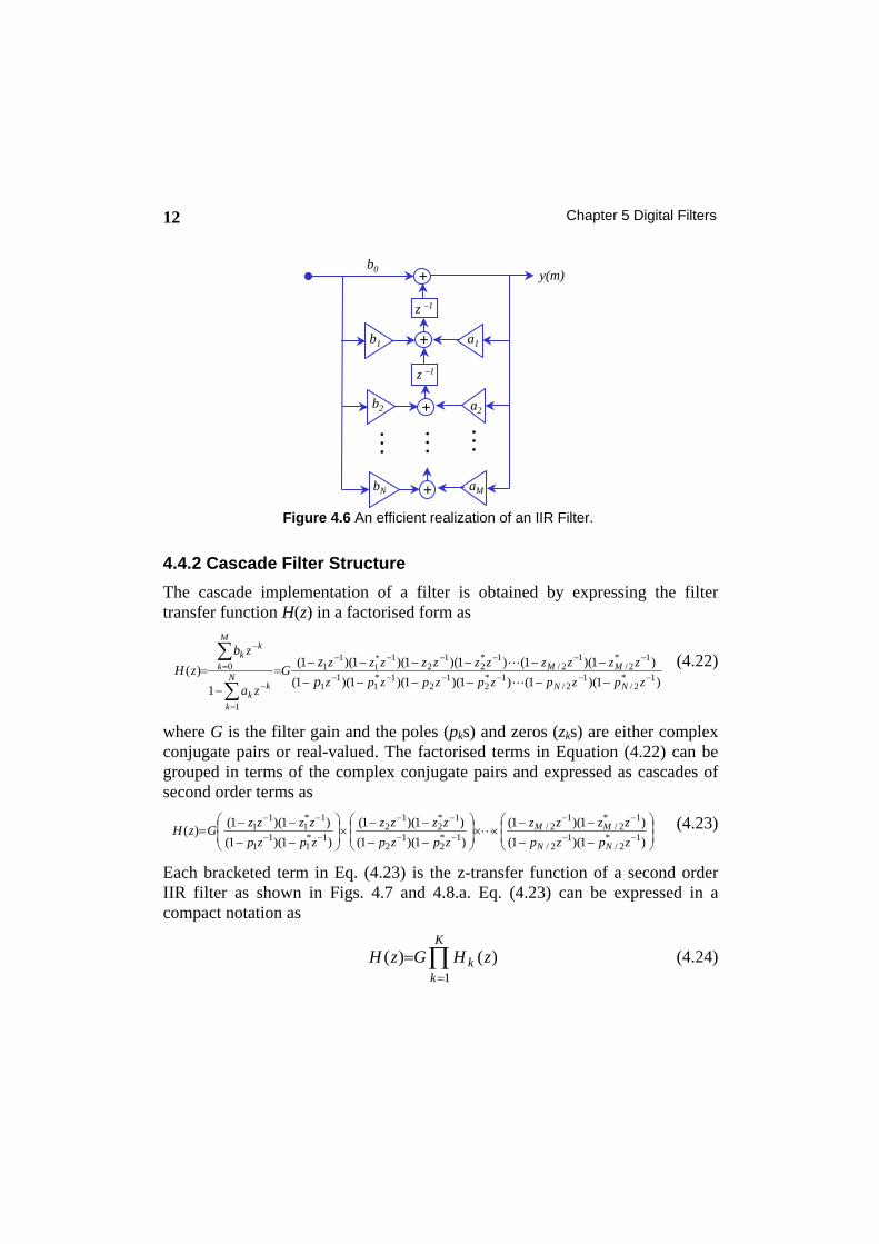
12 Chapter 5 Digital Filters
4.4.2 Cascade Filter Structure
The cascade implementation of a filter is obtained by expressing the filter transfer function H(z) in a factorised form as
)1)(1()1)(1)(1)(1()1)(1()1)(1)(1)(1(
1)( 1*
2/1
2/1*
21
21*
11
1
1*2/
12/
1*2
12
111
1
0*1
−−−−−−
−−−−−−
=
−
=
−
−−−−−−
−−−−−−=
−
=
∑
∑zpzpzpzpzpz
zzzzzzzzzzzGza
zbzH
NN
MMN
k
kk
M
k
kk
pz (4.22)
where G is the filter gain and the poles (pks) and zeros (zks) are either complex conjugate pairs or real-valued. The factorised terms in Equation (4.22) can be grouped in terms of the complex conjugate pairs and expressed as cascades of second order terms as
⎟⎟⎠
⎞⎜⎜⎝
⎛
−−
−−××⎟
⎟⎠
⎞⎜⎜⎝
⎛
−−
−−×⎟
⎟⎠
⎞⎜⎜⎝
⎛
−−
−−= −−
−−
−−
−−
−−
−−
)1)(1()1)(1(
)1)(1()1)(1(
)1)(1()1)(1()( 1*
2/1
2/
1*2/
12/
1*2
12
1*2
12
1*1
11
1*1
11
zpzpzzzz
zpzpzzzz
zpzpzzzzGzH
NN
MM (4.23)
Each bracketed term in Eq. (4.23) is the z-transfer function of a second order IIR filter as shown in Figs. 4.7 and 4.8.a. Eq. (4.23) can be expressed in a compact notation as
∏=
=K
kk zHGzH
1)()( (4.24)
z –1
b0
z –1
a1
a2b2
b1
+
+
+ y(m)
aMbN +
......
...
Figure 4.6 An efficient realization of an IIR Filter.

Sec. 4.4 Filter Structures 13
where for an IIR filter, assuming that N > M, the variable K is the integer part of (N+1)/2 and for an FIR filter K is the integer part of (M+1)/2. Note that a cascade filter may also have one or several first order sections with real-valued zeros and/or real-valued poles and that when N or M are odd numbers there will be at least one first order zero or first order pole in the cascade expression.
For an IIR filter each second order cascade section has the form
22
11
21
11
)(−−
−−
++
++=
zazazbzb
zHkk
kkk (4.25)
For an FIR filter, as shown in Fig. 4.8.b, each second order cascade section has the form
211)( −− ++= zbzbzH kkk (4.26)
z-1
b0
z-1
a1
a2-b2
-b1
+
+
+
z-1
b0
z-1
a1
a2-b2
-b1
+
+
+
z-1
b0
z-1
a1
a2-b2
-b1
+
+
+ g
Figure 4.7 Realization of an IIR cascade structure from second order sections.
z-1
b0
z-1
a1
a2-b2
-b1
+
+
+
z-1z-1
a1 a21
x(m)
y(m) (a) (b)
Figure 4.8 Realization of a second order section of: (a) an IIR Filter, (b) an FIR filter.

14 Chapter 5 Digital Filters
H1(z)
H2(z)
HN(z)
...
+x(m) y(m)
K
Figure 4.9 - A parallel-form filter structure.
4.4.3 Parallel Filter Structure
An alternative to the cascade implementation described in the previous section is to express the filter transfer function H(z), using the partial fraction method, in a parallel form as parallel sum of a number of second order and first order terms as
∑∑=
−=
−−
−
−+
−−+
+=21
11
12
21
1
110
11)(
N
k k
kN
k kk
kk
zae
zazazeeKzH (4.27)
or
∑+
=
+=21
1)()(
NN
kk zHKzH (4.28)
where in general the filter is assumed to have N1 complex conjugate poles, N1 real zeros, and N2 real poles and K is a constant. Figure 4.9 shows a parallel filter structure. MatLab provides a function called (residue z XXX) for conversion of a direct form polynomial to a parallel form polynomial.

Sec. 4.6 Design of Infinite Impulse Response (IIR) Filters 15
4.6 Linear Phase FIR Filters It takes a finite time before the input to a filter propagates through the filter and appears at the output. A delay of T seconds in time domain appears as a phase change of e–j2πT in frequency domain. The time delay, or phase change, caused by a filter depends on the type of the filter (e.g. linear/nonlinear, FIR/IIR) and its impulse response. An FIR filter of order M, with M+1 coefficients, has a time delay of M/2 samples.
A linear phase filter is one whose phase φ(f) is a linear function of the frequency variable f. In the following it is shown that an FIR filter with a symmetric impulse response h(k), or equivalently symmetric coefficients, has a linear phase response. Consider an FIR filter with a symmetric impulse response as
)()( kMhkh −= k = 0, 1, ..., M (4.29)
The frequency response of the filter is the Fourier transform of its impulse response, given by
∑=
−=M
k
fkekhfH0
2j)()( π (4.30)
Expanding Eq. (4.30) and using the assumed symmetry of the filters’ impulse response ⎯ i.e. h(0)=h(M), h(1)=h(M−1) and so on ⎯ we have
⎥⎥⎥
⎦
⎤
⎢⎢⎢
⎣
⎡+−++++=
+−++++=
π−
π−−π−
π
π−ππ−
π−π−−π−π−
))2cos(()1(2
)2(j)2(j
)cos()0(2
jjj
2j1)(j24j2j
)1()1()()0()2/(
)()1()2()1()0()(
fMh
fMfM
fMh
fMfMfM
fMfMff
eMheheMhehMhe
eMheMhehehhfH
(4.31)
where it is assumed that the filter length M+1 is an odd integer. Hence the frequency response of the filter H(f) can be expressed as
( )⎥⎥⎦
⎤
⎢⎢⎣
⎡−+= ∑
−
=
−2/)1(
0
j )2(cos)(2)2/()(M
m
fM fmMmhMhefH ππ (4.32)
The term in the bracket is real-valued. The filter phase is the term e-jMπf, and the filter phase response is given by

16 Chapter 5 Digital Filters
⎩⎨⎧
<+−≥−
=0)(0)(
)(fHiffMfHiffM
fa
a
πππ
φ (4.33)
where Ha(f) is the real-valued term within the bracket of Eq. (4.32). Thus the phase response of an FIR filter with a symmetric impulse response is a linear function of the frequency variable f. When the amplitude of the frequency response Eq. (4.32) goes negative the phase undergoes a change of π radians.
4.6.1 The Location of the Zeros of a Linear Phase FIR Filter The transfer function of an FIR filter with a symmetric impulse response [h(0)=h(M), h(1)=h(M-1) … ] can be rearranged and written as
)()(
)0()1()(
)()1()0()()(
1
0
10
1
−−
=
−
−−=
−−−
==
++−+=
+++==
∑
∑
zHzzmhz
zhzMhMh
zMhzhhzmhzH
MM
m
mM
M
M
m
Mm
(4.34)
Form Eq. (4.34) we have the relationship H(z)= z-MH(z-1) which implies that if H(z) has a zero at z=z1 then it must also have a zero at z=1/z1. Therefore, in general the z-transfer function of a linear phase FIR filter can be factorized as
pairzeroResiprocal
11
11
pairzeorconjugateComplex
11
11 ))/1(1)()/1(1()1)(1()( 1111 −−−−−− −−−−= zerzerzerzerGzH jjjj ϕϕϕϕ (4.35)
where rk and ϕk are the radius and angular frequency of the kth complex pair of zeros. Thus the zeros of a linear phase filter occur in reciprocal pairs mirrored w.r.t. the unit circle, the exception being when the zeros are on the unit circle.
Example 4.1 The input-output relationship of a finite impulse response filter is given as
)4()3(5.2)2(25.5)1(5.2)()( −+−−−+−−= mxmxmxmxmxmy (4.36)
(i) Write the z-transfer function of this filter.
(ii) Show that the filter has a linear phase response.

Sec. 4.6 Design of Infinite Impulse Response (IIR) Filters 17
(iii) Find and plot the zeros of this filter and explain the constraints on the position of the zeros of a linear phase filter.
Solution: The z-transfer function of the finite impulse response filter H(z) is given by
4321 5.225.55.21)( −−−− +−+−= zzzzzH (4.37)
( ) ( )[ ]fffff
ffff
eeeee
eeeefHπππππ
ππππ
2j2j4j4j4j
8j6j4j2j
5.25.225.5
5.225.55.21)(−−−
−−−−
+−++=
+−+−= (4.38)
Hence the frequency response of the filter H(f) can be expressed as
[ ])2cos(5)4cos(225.5)( 4j ffefH f π−π+= π− (4.39)
The filter’s phase response is given by
⎩⎨⎧
<+−≥−
=0)(40)(4
)(fHifffHiff
fa
a
πππ
φ (4.40)
where Ha(f) is the real-valued term within the bracket of Eq. (4.45). The transfer function H(z) can be factorized as
Re
Im
r
1/r
Figure 4.10 Symmetric structure of the zeros of a linear phase FIR filter

18 Chapter 5 Digital Filters
( )( )( )( )( )( )13/13/13/13/
2121
21215.015.01
42125.05.01)(−−−−−−
−−−−
−−−−=
+−+−=
zezezeze
zzzzzHjjjj ππππ
(4.41)
The zeros of the filter are positioned at a radii of 0.5 and 2 and angles of ±60 as shown in Fig. 4.10.
Example 4.2 Consider a unit delay filter with the following impulse response
⎩⎨⎧ =
=−=otherwisem
mmh0
11)1()( δ
(4.42)
The frequency response of the filter is obtained as the Fourier transform of the impulse response as
fmfM
meemhfH ππ 2jj2
0)()( −−
=== ∑ (4.43)
The filter magnitude frequency response is
1|||)(| 2j == − fefH π (4.44)
and the filter phase response is ff πφ 2)( −= (4.45)
1.0
0.0
Fs/2Frequency
1.0
0.0
Fs/2Frequency0
0
-3.5
Frequency Fs/20
0
-3.5
Frequency Fs/2
Mag
nitu
de(f)
Phas
e(f)
Figure 4.11 Magnitude frequency and phase response of a unit delay filter.
h(m)
m0 1
z – 1x(m) y(m)

Sec. 4.6 Design of Infinite Impulse Response (IIR) Filters 19
This filter has a unity magnitude response and a linear phase response shown in Fig. 4.11. This is called a pure delay filter as its only effect is to delay the input.
Example 4.3 Consider a filter with the following impulse response
⎩⎨⎧ =
=−=otherwise
KmKmmh
01
)()( δ
(4.46)
The frequency response of the filter is obtained as the Fourier transform of the impulse response as
fKmfM
meemhfH ππ 2j2j
0)()( −−
=== ∑ (4.47)
The filter magnitude response is
1|||)(| 2j == − KfefH π (4.48)
and the filter phase response is
fKf πφ 2)( −= (4.49)
This filter has a unity magnitude response and a linear phase response. This is a pure delay filter as its only effect is to delay the input by k samples. In the phase plot of Fig. 4.12, at the frequency of zero Hz the phase φ(0)=0, at f=1/2k the phase is φ(1/2k )= −π. The phase plot shows the periodic circular nature of the phase in that ej(−π−φ) =ej(2π−π−φ) =ej(π−φ) , so that there is a jump to π whenever the phase becomes smaller (more negative) that −π as shown in Fig. 4.12.
0
1
Fs/2Frequency 0-4
-2
0
2
4
Frequency Fs/2
Phas
e(f)
Mag
nitu
de(f)
c
1
Figure 4.12 Magnitude and phase response of a delay filter with a delay of 10-units.
z – Kx(m) y(m)
h(m)
m0 K

20 Chapter 5 Digital Filters
Example 4.4 Consider a filter with the following impulse response
)()()( Kmmmh −+= δδ (4.50)
The frequency response of the filter is obtained as the Fourier transform of the impulse response as
)cos(2)(
1)()(
jjjj
2j2j
0
fKeeee
eemhfH
fKfKfKfK
fKmfM
m
πππππ
ππ
−−−
−−
=
=+=
+== ∑ (4.51)
This filter’d magnitude frequency response is comb-shaped and given by
)cos(2)cos(2)( j fKfKefH fK πππ == − (4.52)
and the filter phase response is fKf πφ −=)( (4.53)
Fig. 4.13 shows the filter magnitude and the phase responses for a value of K=4.
h(m)
mK0
11
x(m)
y(m)
z – K
Frequency Fs/2
Mag
nitu
de(f)
0-2
0
2
Frequency Fs/2
Phas
e(f)
Figure 4.13 Magnitude frequency and phase response of a comb filter.

Sec. 4.6 Design of Infinite Impulse Response (IIR) Filters 21
Example 4.5 Consider a filter with the following impulse response
⎩⎨⎧ =
=otherwisem
mh0
10...,,1,01)( (4.54)
The filter length is 11 samples long. The frequency response of this filter is obtained from the Fourier transform of the impulse response and using the convergence formula for a geometric series, as
)sin()11sin(
11)( 10j
jj
11j11j
j
11j
2j
22j10
0
2j
ffe
eeee
ee
eeefH f
ff
ff
f
f
f
f
m
fmTs
πππ
ππ
ππ
π
π
π
ππ −
−
−
−
−
−
−
=
− =−−
×=−−
== ∑ (4.55)
and the filter phase response is
⎩⎨⎧
<+−≥−
=0)(100)(10
)(fHifffHiff
fa
a
πππ
φ (4.56)
where )sin(/)11sin()( fffH a ππ= . Note that at f=0, H(f)=sin(Af)/sin(Bf)=0/0 is undefined, and is obtained as H(f)=Acos(Af)/Bcos(Bf)=A/B. Notice two trends in the phase response plot of Fig. 4.14. First, note that at the points when
)( fH a changes sign (a change of sign is equivalent to multiplying Ha(f) by –1 or πje ) there is a sudden jump of π in phase. Second, depending on the filter coefficients, )( fH a may change sign before fe π10j− attains a phase of −π, −2π ... causing a gradual positive shift in the phase as shown in the ramp trend of Fig. 4.14.
h(m)
m
00
2
4
6
8
10
12
Frequency Fs/2
|Mag
nitu
de(f)
|
0-3-2.5-2.0-1.5-1.0-0.50.00.51.0
1.5
Phas
e(f)
Frequency Fs/2 Figure 4.14 Magnitude and phase response of filter with a rectangular impulse response.

22 Chapter 5 Digital Filters
4.6.2 Design of FIR Filters by Windowing A simple way to design an FIR filter is through the inverse Fourier transform of the desired frequency response. Consider an FIR filter described by the difference equation
∑=
−=M
kk kmxbmy
0)()( (4.57)
where bks are the filter coefficients, M is the filter order, and x(m) and y(m) are the filter’s input and output signals respectively. Now, when an FIR filter Eq. (4.57) is excited with an impulse input then it is easy to see, as shown in Fig. 4.2, that the impulse response of the FIR filter is identical to the coefficients sequence of the filter {bk} that is:
⎩⎨⎧ ≤≤
=Otherwise
Mkbkh k
00
)( (4.58)
Hence the filtering Eq. (4.58) can be expressed as the convolution of the impulse response of the FIR filter h(m) with the input signal x(m) as
∑=
−=M
kkmxkhmy
0)()()( (4.59)
This observation forms the basis for the method of FIR filter design by windowing. In the window design method we begin with the desired frequency response Hd(f) and obtain the corresponding impulse response hd(m) which, for an FIR filter, is the filter coefficients.
The frequency response Hd(f) and the impulse response hd(m) of a linear filter are related by the Fourier transform pair as
∑=
π−=M
m
fmdd emhfH
0
2j)()( (4.60)
∫−
π=2/1
2/1
2j)()( dfefHmh fmdd (4.61)
Thus given the desired filter frequency response Hd(f) we can determine the impulse response hd(m) by evaluating the above Fourier integral. However,

Sec. 4.6 Design of Infinite Impulse Response (IIR) Filters 23
there are two problems here. First, the filter has infinite duration impulse response. Second, the filter is non-causal, as it will have non-zero values for coefficients with negative time index. Note a negative-indexed coefficient e.g. h(-k) requires a future sample value x(m+k), this makes the filter non-causal for real-time operations. These problems are solved by first multiplying hd(m) by a truncation window of length (M+1) samples, and then shifting the truncated impulse response by M/2 samples in the positive time direction.
The FIR filter window design technique involves the following steps:
(1) Start with the desired frequency response Hd(f).
(2) Choose a filter order M.
(3) Obtain hd(m) the inverse Fourier transform of Hd(f), From Eq. (4.61).
(4) Window hd(m) to obtain M+1 FIR filter coefficients centred at m=0.
(5) Shift the windowed impulse response by M/2 samples for causality.
4.6.3 The Influence of the Choice of Window in FIR Filter Design After windowing the impulse response of the FIR filter can be described as
)()()( mhmwmh d= (4.62)
Since multiplication in time is equivalent to convolution in the frequency domain, the frequency response H(f) of the truncated FIR filter h(k) is given by
∫−
−=2/1
2/1
)()()( ϕϕϕ dfWHfH d (4.63)
where W(f), the frequency response of a rectangular window w(m), is obtained from a Fourier transform. Using the convergence formula for a geometric series, W(f) can be expressed as
( ))sin()1(sin
11)()( j
2j
)1(2j
0
2jf
fMee
eemwfW fMf
fMM
m
fmπ
π+=
−
−== π−
π−
π+−
=
π−∑ (4.64)
Note that at f=0, W(f)=sin(Af)/sin(Bf)=0/0 is undefined, and is obtained as W(f)=Acos(Af)/Bcos(Bf)=A/B. The sinc-shaped magnitude spectrum of the rectangular window is illustrated in Fig. 4.14.a for M = 32, 128. The bandwidth of the main lobe is 2Fs/M, where Fs is the sampling frequency.

24 Chapter 5 Digital Filters
The convolution of the rectangular window W(f) with the filter Hd(f) has the effects of introducing ripples in the frequency spectrum of the filter and extending the transition regions of the filter. As the filter order M increases the main lobe width and the amplitude of the side lobes decrease.
The side lobes in the frequency domain are manifestation of the discontinuities in time domain at the edges of a rectangular window and can be alleviated by the use of windows that do not contain sharp discontinuities and roll down rather gently to zero such as the raised-cosine windows of Hamming, Hanning, and Blackman windows described in section 3.xx and reproduced here for convenience. The general form of the raised cosine window equation is given by
( )⎪⎩
⎪⎨⎧ ≤≤
+−−
=otherwise
MmM
mmw
0
01
2cos1)(
παα (4.65)
For α=0.5 we have the Hanning window:
MmM
mmwHan ≤≤+
−= 01
2cos5.05.0)( π (4.66)
For α=0.54 we have the Hamming window
MmM
mmwHam ≤≤+
−= 01
2cos46.054.0)( π (4.67)
The Blackman window is given by
MmM
mM
mmwBlack ≤≤+
−+
−= 01
4cos08.01
2cos5.042.0)( ππ (4.68)
Fig 4.15 shows the rectangular, the Hamming and the Blackman windows. Fig. 4.15 shows the spectra of these windows for two different window length of M=32 and M=128. Figure 4.16 shows the frequency spectrum of three different widows for window lengths of 32 samples and 128 samples. As shown the Blackman window has considerably smaller side-lobes but at the expense of a higher bandwidth of the main-lobe.
function WindowsResponse( )
% This function draws the shape of a window and its frequency response

Sec. 4.6 Design of Infinite Impulse Response (IIR) Filters 25
0 2 0 4 0 6 0 8 0 1 0 0 1 2 0 1 2 80
0 . 1
0 . 2
0 . 3
0 . 4
0 . 5
0 . 6
0 . 7
0 . 8
0 . 9
1
Am
plitu
de
T i m e
H a m m i n gR e c t a n g l e
B l a c k m a n
Figure 4.15 Plot of: (a) rectangular window, (b) Hamming window, (c) Blackman window for a window length of 32 samples (left) and 128 samples.
(a) 0
-60
-50
-40
-30
-20
-10
0
20 lo
g 10|W
(f)|
dB
Frequency HzFs/2
0
Frequency HzFs/2
-60
-50
-40
-30
-20
-10
0
20 lo
g 10|W
(f)|
dB
(b) 0 Frequency Hz Fs/2
-60
-50
-40
-30
-20
-10
0
20 lo
g 10|W
(f)|
dB
-60
-50
-40
-30
-20
-10
0
20 lo
g 10|W
(f)|
dB
Frequency Hz Fs/20

26 Chapter 5 Digital Filters
(c) Frequency Hz0-80
-60
-50
-40
-30
-20
-10
0
20 lo
g 10|W
(f)|
dB
-70
Fs/2 -80
-60
-50
-40
-30
-20
-10
0
20 lo
g 10|W
(f)|
dB
-70
Frequency Hz Fs/20
Figure 4.16 The spectra of: (a) rectangular window (b) Hamming window, (c) Blackman window for a window length of 32 samples (left) and 128 samples (right).
4.6.4 Design of a Low Pass Linear-Phase FIR Filter Using Windows Example 4.6 Consider the design of a low-pass linear-phase digital FIR filter operating at a sampling rate of Fs Hz and with a cutoff frequency of Fc Hz. The frequency response of the filter is given by
⎩⎨⎧ <
=otherwise
FffH c
d 0||0.1
)( (4.69)
The impulse response of this filter is obtained via the inverse Fourier integral as
( )m
mFm
edfemh cF
F
fmF
F
fmd
c
c
c
cππ
=π
==−
π
−
π∫2sin
2j0.1)(
2j2j (4.70)
Clearly hd(m) is of infinite duration and non-causal as it is none-zero valued for m < 0 and. Note that in the FIR filter Equation (4.12) a negative index value of h(-m) such as h(-10) would require a future sample value x(m+10) hence it is non-causal.
H(f)
Fc–Fc
1

Sec. 4.6 Design of Infinite Impulse Response (IIR) Filters 27
To obtain an FIR filter of order M we multiply hd(m) by a rectangular window sequence of length M+1 samples centered at m=0. To introduce causality (h(m)=0 for m < 0) shift h(m) by M/2 samples
( )
MmMm
MmFmh c ≤≤
−π−π
= 0)2/(
)2/(2sin)( (4.71)
The impulse response and frequency response of a low pass filter for the filter
0 5 10 15 20 25 30-0.2
-0.1
0
0.1
0.2
0.3
0.4
0.5
0 20 40 60 80 100-0.2
-0.1
0.0
0.1
0.2
0.3
0.4
0.5
Time m0
0.2
0.4
0.6
0.8
1.0
1.2
Frequency fs/2
h(m
)
|H(f)
|
0.2
0.4
0.6
0.8
1.0
1.2
Frequency fs/20
|H(f)
|
0 20 40 60 80 100-0.2
-0.1
0.0
0.1
0.2
0.3
0.4
0.5
h(m
)
Time m
Time m
Time m
h(m
)
|H(f)
|
0
0.2
0.4
0.6
0.8
1.0
1.2
Frequency fs/2
(a)
(b)
(c)
Figure 4.17 The impulse response and the magnitude frequency response of an FIR filter for the following cases: (a) filter order 30 with a rectangular window, (b) filter order 100 with a rectangular window, (c) filter order 100 with a hamming window.

28 Chapter 5 Digital Filters
orders of M=30 and M=100 are shown in Fig 4.17. Observe the relatively large oscillations or the ripples in the pass-band and the stop-band. These ripples increase in frequency as M the filter order is increased. These oscillations are a direct result of the convolution with the side-lobes of the rectangular window.
To reduce the ripples in both the pass-band and the stop-band we can use a window function that decays to zero gradually instead of the abrupt discontinuous transition that happens at the edges of a rectangular window.
Fig 4.17.b illustrates how the use of a Hamming window reduces the ripples in the pass-band and the stop-band. The ‘price’ paid is an increase in the bandwidth of the transition band.
4.6.5 Design of High-Pass FIR Filters
Example 4.7 Consider the design of a high-pass linear-phase digital FIR filter operating at a sampling rate of Fs Hz and with a cutoff frequency of Fc Hz. The frequency response of the filter is given by
⎩⎨⎧ <
=otherwise
FffH c
d 0.1||0
)(
(4.72)
The impulse response of this filter is obtained via the inverse Fourier integral as
( ) ( )π
π−
ππ
=
π+
π=+=
π−
−
ππ
−
−
π ∫∫
mFFm
mm
me
medfedfemh
sc
FF
fmFFfm
FF
fmFF
fmd
sc
sc
sc
sc
/2sinsin
2j2j0.10.1)(
5.0
/
2j/
5.0
2j5.0
/
2j/
5.0
2j
(4.73)
The impulse response hd(m) is non-causal (it is nonzero for m < 0) and infinite in duration. To obtain an FIR filter of order M we multiply hd(m) by a rectangular window sequence of length M+1 samples. To introduce causality (h(m) =0 for m < 0) shift truncated h(m) by M/2 samples
H(f)
Fc–Fc
1

Sec. 4.6 Design of Infinite Impulse Response (IIR) Filters 29
( ) ( )π−
−π−
π−−π
=)2/(
/)2/(2sin)2/(
)2/(sin)(Mm
FFMmMm
Mmmh sc (4.74)
Note that a high-pass FIR filter is also equivalent to the configuration shown in the Fig. 4.18.
4.6.6 Design of Band-Pass FIR Filters Example 4.8 Consider the design of a band-pass linear-phase digital FIR filter operating at a sampling rate of Fs Hz and with a lower and higher cutoff frequencies of FL and FH Hz. The frequency response of the filter is given by
⎩⎨⎧ <<
=otherwise
FfFfH HL
d 0||1
)( (4.75)
The impulse response of this filter is obtained via the inverse Fourier integral as
( ) ( )m
FFmm
FFm
me
medfedfemh
SLSH
FF
FF
fmFF
FF
fmFF
FF
fmFF
FF
fmd
SH
SL
SL
SH
SH
SL
SL
SH
ππ
−π
π=
π+
π=+=
π−
−
ππ
−
−
π ∫∫
/2sin/2sin
2j2j0.10.1)(
/
/
2j/
/
2j/
/
2j/
/
2j
(4.76)
H( f )
f–FL
1
–FHFL FH
Delay of M/2
++
–
Figure 4.18 Design of a high-pass FIR filter from a low-pass filter.

30 Chapter 5 Digital Filters
The impulse response hd(m) is non-causal (it is nonzero for m < 0) and infinite in duration. To obtain an FIR filter of order M multiply hd(m) by a rectangular window sequence of length M+1 samples. To introduce causality (h(m) =0 for m < 0) shift truncated h(m) by M/2 samples
( ) ( )π−
−π−
π−−π
=)2/(
/)2/(2sin)2/(
/)2/(2sin)(
MmFFMm
MmFFMm
mh sLsH (4.77)
Note that a high-pass FIR filter is equivalent to the configuration shown in the Fig. 4.19.
+–
+
Figure 4.19 Design of a band-pass FIR filter from a low-pass FIR filters
4.6.7 Design of Band-Stop FIR Filters Example 4.9 Consider the design of a band-stop linear-phase digital FIR filter operating at a sampling rate of Fs Hz and with a lower and higher cutoff frequencies of FL and FH Hz. The frequency response of the filter is given by
⎩⎨⎧ <<
=otherwise
FfFfH HL
d 1||0
)( (4.78)
The impulse response of this filter is obtained via the inverse Fourier integral as
H( f )
f–FL
1
–FHFL FH

Sec. 4.6 Design of Infinite Impulse Response (IIR) Filters 31
mFmF
mFmF
mm
dfedfedfemh
sLsH
FF
fmFF
FF
fmFF
fmd
sH
sL
sL
sH
ππ
ππ
ππ
πππ
/2sin/2sinsin
0.10.10.1)(5.0
/
2j/
/
2j/
5.0
2j
+−=
++= ∫∫∫−
−
− (4.79)
The impulse response hd(m) is non-causal (it is nonzero for m < 0) and infinite in duration. To obtain an FIR filter of order M we multiply hd(m) by a rectangular window sequence of length M+1 samples. To introduce causality (h(m) =0 for m < 0) shift h(m) by M/2 samples
π−−π
+π−
−π−
π−−π
=)2/(
/)2/(2sin)2/(
/)2/(2sin)2/(
)2/(sin)(Mm
FFMmMm
FFMmMm
Mmmh sLsH
(4.80)
Note that a band-pass FIR filter is also equivalent to the configuration shown in the Figure 4.20.
function DrawFIR_WindowsResponse() % This function draws the impulse response and the frequency response of an FIR % filter with a selection of different types of frequency response (lowpass, highpass, % bandpass, bandstop)and windows. The filter design parameters are filtertype, % window, filter cutoff frequencies and filter order.
+–
+−π π
− FL FL
FH− FH
+
Figure 4.20 Design of a band-stop FIR filter from low-pass FIR filters.

32 Chapter 5 Digital Filters
4.7 Design of Digital FIR Filter-banks Filter-banks have many applications in signal processing and communication such as in sub-band signal coding, music coders (MPEG and ATRAC), multi-rate communication systems, frequency multiplexing, noise reduction systems and audio graphic equalizers.
In it conventional form a filter-bank is a parallel configuration of band-pass filters as shown in Fig. 4.21. The sub-band filters may be uniformly spaced in the frequency domain or they may be spaced non-uniformly according to the energy contents of the various bands and/or the human perception of the signals in critical bands of hearing. For example in speech processing it is common to use a perceptually based non-uniform spacing of the sub-band filters such that increasingly higher frequency bands have increasingly larger bandwidths.
The band-pass filters that form a filter-bank can be FIR filters, or IIR filters such as band-pass Butterworth filters. The following example demonstrates a simple procedure for the design of a four-band filter-bank using FIR filters.
Example 4.10 Design of an FIR Filter-bank Design a bank of digital FIR filters for a telephony speech application to split a total bandwidth of 4 kHz into 4 equal bandwidth sub-bands.
Solution: Assume the sampling frequency is 8 kHz. For uniformly spaced band-pass filters the filter cutoff points for the four band-pass filters are 0 and 1
Figure 4.21 A block diagram illustration of a four-bands filter-bank.

Sec. 4.6 Design of Infinite Impulse Response (IIR) Filters 33
kHz, 1 and 2 kHz, 2 and 3 kHz, and 3 and 4 kHz respectively.
First, we design a low-pass filter with a bandwidth of 1 kHz. At a sampling rate of Fs=8 kHz, a frequency of 1 kHz corresponds to a normalized angular frequency of ωN=2π×f/Fs=π/4 radians or a normalized frequency of fN==f/Fs=1/8=0.124. Using the window design technique the FIR impulse response is obtained from the inverse Fourier transform as
∫−
=125.0
125.0
2j0.1)( dfemh fmd
π (4.81)
Using the solution described in section 4.xx we obtain the windowed FIR filter response as
))2/(25.0(sinc25.0)()(1 Mmmwmh −×= π 0 ≤ m ≤ M (4.82)
To design the band-pass filters we can use the amplitude modulation (AM) method to translate a low-pass filter to a band-pass filter. For a band-pass width of 1 kHz the low-pass filter should have cutoff frequencies of ±500 Hz (note that from –500 to +500 Hz we have a bandwidth of 1 kHz). Thus the required low pass FIR filter equation is similar to Eq. (4.82), but with half the bandwidth, and its impulse response is given by given by
( ))2/(125.0sinc125.0)()( Mmmwmh −π×= 0 ≤ m ≤ M (4.83)
To translate this low pass filter to the specified band pass filters we need AM sinusoidal carriers with frequencies 1.5 kHz, 2.5 kHz and 3.5 kHz. The modulated band pass filter equations are given by
( ) )8/3(sin)2/(125.0sinc125.0)(2)(2 mMmmwmh π−π××= 0≤ m ≤M (4.84)
( ) )8/5sin()2/(125.0sinc125.0)(2)(3 mMmmwmh π−π××= 0≤ m ≤M (4.85)
( ) )8/7(sin)2/(125.0sinc125.0)(2)(4 mMmmwmh π−π×= 0≤ m ≤M (4.86)
The process of amplitude modulation halves the amplitude of each sideband, hence we have the multiplying factor of 2 in Eqs (4.84-4.86).
function filterbank( )
% Designs a bank of N equal bandwidth FIR filters.

34 Chapter 5 Digital Filters
00
0 . 2
0 . 4
0 . 6
0 . 8
1
F s / 2F r e q u e n c y Figure 4.22 The frequency spectrum of a four-band FIR filter.
0- 0 .1
- 0 .0 5
0
0 .0 5
0 .1
0 .1 5
0 .2
0 .2 5
F r e q u e n c y F s / 20- 0 .1
- 0 .0 5
0
0 .0 5
0 .1
0 .1 5
0 .2
0 .2 5
F r e q u e n c y F s / 2 0- 0 . 2 5
- 0 .2
- 0 . 1 5
- 0 .1
- 0 . 0 5
0
0 .0 5
0 .1
0 .1 5
0 .2
F r e q u e n c y F s / 2
0- 0 .2 5
- 0 . 2
- 0 .1 5
- 0 . 1
- 0 .0 5
0
0 .0 5
0 .1
0 .1 5
0 .2
0 .2 5
F r e q u e n c y F s / 2 0- 0 .2
- 0 .1 5
- 0 .1
- 0 .0 50
0 .0 5
0 .1
0 .1 5
0 .2
0 .2 5
F s / 2F r e q u e n c y Figure 4.23 The impulse response of the individual band-pass filters of a 4-band filter-
bank, plotted clockwise from the top left corner for bands 1 to 4.
4.4.1 Quadrature Mirror Subband Filters Quadrature mirror filters are used to construct a filter bank for spliting a signal into a number of sub-band signals for applications such as sub-band music coding or wavelet analysis.
A quadrature mirror filter, shown in Figure 4.24, splits an input signal into two equal width sub-band signals composed of a lowpass sub-band signal and a highpass sub-band signal. The sub-band signals are then downsampled by

Sec. 4.6 Design of Infinite Impulse Response (IIR) Filters 35
a factor of 2. After downsampling, the upper band has inverted frequencies, i.e. the low frequencies appear at the high frequencies and vice versa.
The filterbank of Figure 4.24 consists of a lowpass filter, H0(z), a highpass filter H1(z), downsamplers, a DSP process (for such functions as coding, noise reduction etc.), upsamplers and antialiasing filters G0(z) and G1(z). The lowpass filter H0(z) and the highpass filter H1(z), split the input signal into low frequency and high frequency bands. Both subband signals are then downsampled by a factor of 2.
The z-transform of a signal down-sampled by a factor of 2 can be expressed as
1/ 2 1/ 21( ) ( ) ( )2dX z X z X z⎡ ⎤= + −⎣ ⎦ ()
Note that the realtion is true because / 2
1/ 2 1/ 2 2( ) ( )
0
kk k z for k even
z zotherwise
⎧+ − = ⎨
⎩ ()
After filtering and dowsampling, the z-transforms of the lowpass and highpass subband signals, denoted as X0d(z) and X1d(z) respectively, can be expressed as
[ ]0 0 0 01( ) ( ) ( ) ( ) ( ) ( )2
X z G z H z X z H z X z= + − − (4.87 )
[ ]1 0 1 11( ) ( ) ( ) ( ) ( ) ( )2
X z G z H z X z H z X z= + − − (4.87 )
[ ] [ ]0 1
0 0 1 1 0 0 1 1
( ) ( ) ( )1 1( ) ( ) ( ) ( ) ( ) ( ) ( ) ( ) ( ) ( )2 2
Aliasing Term
X z X z X z
G z H z G z H z X z G z H z G z H z X z
= +
= + + − + − −
(4.87 )
For perfect reconstruction we need o have
0 0 1 1( ) ( ) ( ) ( ) 0G z H z G z H z− + − = ( )
For Equation to be true we need to have
0 1( ) ( )G z H z= − and 1 0( ) ( )G z H z= − − ( )

36 Chapter 5 Digital Filters
∑∞
−∞=++=
kssd kFfHkFfXfX )2/()2/()( 00 (4.87 )
∑∞
−∞=++=
kssd kFfHkFfXfX )2/()2/()( 11 (4.88 )
Figure 14.24 illustrates the spectrum of a full band signal and also the spectra of the lowpass and higpass sub-bands before and after downsampling by a factor of 2 to 1. Note that whereas the spectrum of the fullband signal has a bandwidth of Fs and a repeatition period of Fs, the spectra of the subband signals after downsampling by a factor of 2 have a bandwidth of Fs/2 and a repeatition period of Fs/2.
To reconstruct the signal, both sub-band signals are upsampled by a factor of 2, and filtered with anti-aliasing filters G0(f) and G1(f). Thus, the reconstructded output can be written as
H1( f ) 2:1
H0( f ) 2:1
X1(f), Fs/4 <f < Fs/2
DigitalSignal
Processor
1:2
1:2
G1( f )
G0( f )
X0(f),Fs/4 <f < Fs/2
+X(f)
X(f)^
Figure 4.24 - A QMF filter splitting a signal into two equal bandwidth sub-bands. For reconstruction the individual subband signals are upsampled and filtered by anti-aliasing filters.

Sec. 4.6 Design of Infinite Impulse Response (IIR) Filters 37
[ ]
[ ]aliasing
1100
1100
)2/()()2/()()2/(21
)()()()()(21)(ˆ
sss FfXfGFfHfGFfH
fXfGfHfGfHfX
++++
++=
(4.89)
where for notational convenience the sampling frequency Fs (e.g. 44100Hz for music) is usually normalised to 1. Note that as a result of downsampling by a factor of 2 and then later upsampling by a factor of 2, each frequency f will have an aliasing term X(f+Fs/2). For cancellation of the aliasing term, we require thefollowing relationships between the frequency response of the subband filters H0(f) and H1(f) and the antialiasing filters G0(f) and G1(f):
X ( f )
X 0 ( f ) = H 0 ( f ) X 0 ( f )F s- F s
X 0 d ( f )
X 1 d ( f )
f
f
f
f
f0
( a )
( b )
( c )
( d )
( e )
X 1 ( f ) = H 1 ( f ) X ( f )
Figure 4.25 Illustration of dividing a signal into two subbands: (a) the original signal, (b) the lower half-band, (c) the upper half-band, (d) the lower half-band after down-sampling, and (e) the upper half-band after down-sampling.
Note that as a result of downsampling a signal by a factor Fs/2 and the consequent aliasing X(f+Fs/2) becomes X(f). Hence after downsampling the higher frequencies of the upperband signal (c) appear at the lower frequencies in (d) and vice versa.???????

38 Chapter 5 Digital Filters
)2/()( 10 sFfHfG += (4.90)
)2/()( 01 sFfHfG +=− (4.91)
we also require
[ ] 1)()()()(21
1100 =+ fHfGfHfG (4.92)
so that perfect reconstruction is achieved.
The aliaising cancellation may not work perfectly in the presence of quantization noise. To get good reconstruction without relying on the aliasing cancellation, the QMF filters need to have a steep pass-to-stop-band transition.
QMF filters can be constrcuted by designing a low pass filter with a cutoff frequency of Fs/4 and then inverting the sign of the odd-indexed coefficients − this has the effect of mirroring the poles and zeros − to produce a high pass filter.
Splitting a signal into more than two subbands can be performed by using a binary tree structure of QMF filters where a set of two QMF filters (a lowpass and a highpass) combined with down sampler/s are used several times in a tree-like structure to progressively divide the frequency spectrum and achieve finer bandsplitting as illustrated in Figures (4.25 and 4.26).
function QMF( )
% Function QMF is a simple 2 band filter designed from a low pass FIR filter
H1( f ) 2:1
H0( f ) 2:1
2:1
X(f), Fs/4<f < Fs/2
X(f), Fs/8<f < Fs/4
X(f), 0<f < Fs/4
H1( f )
H0( f )
2:1
X(f), 0 <f < Fs/8
Figure 4.26 A tree-based method for dividing a signal into three sub-bands.

Sec. 4.6 Design of Infinite Impulse Response (IIR) Filters 39
Example 4.11 - Design of Tree-structured FIR Filter-bank Using the digital FIR low pass filter and a binary-tree structure design a bank of filters, operating at a sampling rate of 44100, to divide a total bandwidth of 22.05 kHz into three bands of 0-4.5125 kHz, 4.5125-11.025 kHz and 11.025-22.05 kHz. We start by designing a lowpass filter with a cutoff frequency of 11.025 kHz, which at a sampling rate of 44.1 kHz translates to a normalized cutoff frequency of
fc=11.025/44.1=0.25 Using the window design technique the FIR filter impulse response is obtained from the inverse Fourier transform as
∫−
=fc
fc
fmjd dfemh π20.1)(
(4.93)
we obtain the FIR low-pass filter response as
( ))2/(5.0sinc5.0)()(1 Mmmwmh −×= π 0 ≤ m ≤ M (4.94)
Figure 4.26 shows the configuration of tree-structured filter bank constructed from a combination of a lowpass filter unit, delays and down samplers. Note that after down sampling, the lowpass band is further subdivided into two bands by the repeated application of the lowpass filter.
z -M/2
2:1
2:1
11.025-22.05 kHz
0.0-5.5125 kHz
5.5125-11.025 kHz
2:1
11.025-22.05 kHz
0.0-5.5125 kHz
5.5125-11.025 kHzz -M/2
Figure 4.27 The configuration of a filter bank to split a total bandwidth of 22.05 kHz into three bands of 0-4.5125 kHz, 4.5125-11.025 kHz and 11.025-22.05 kHz.

40 Chapter 5 Digital Filters
4.8 Design of Infinite Impulse Response (IIR) Filters by Pole-Zero Placements
Filter design by pole-zero placements is a useful method for simple applications such as the design of a notch filter and pre-emphasis and de-emphasis filters. Filter design by pole-zero placements is also illustrative of the effects of zeros or poles on shaping the spectrum of the filter response. As described in section 3.xx the effect of a pair of complex zeros is to introduce a trough in the frequency domain and the effect of a pair of complex poles is to introduce a resonance. In the following examples we describe simple filter design techniques by pole-zero placements.
Example 4.12 - Design of an IIR Notch Filter Design a notch filter, operating at a sampling rate of 20 kHz, with a zero magnitude response at 5 kHz, a 3dB stop-band bandwidth of 100 Hz and unity response at frequencies of 0 and 10 kHz.
Solution: The normalized angular frequency can be obtained from ω=2πf/Fs, with Fs=20 kHz. The frequencies of 0, 5 kHz, and 10 kHz correspond to 0, π/2 and π radians respectively.
The specification given is H(0)=H(π)=1 and H(π/2)=0. The 3dB point frequencies are 4950 Hz and 5050 Hz corresponding to the angular frequencies of
200994950
2000023 ππφ ==dB
low and 200
101505020000
23 ππφ ==dBupper (4.95)
To obtain a zero magnitude response at an angular frequency of π/2, corresponding to a frequency of 5 kHz at a sampling rate of 20 kHz, we need a pair of unit-radius complex zeros at e j± π /2 . The corresponding z-transfer function is given by
212/12/ 1)1)(1()( −−−− +=−−= zzezezH jj ππ (4.96)

Sec. 4.6 Design of Infinite Impulse Response (IIR) Filters 41
To control the bandwidth of the notch filter we place a pair of poles on the same frequency as the notch frequency as shown in Figure 4.28. The resulting transfer function is
22
2
11)(
−
−
+
+=
zrzgzH (4.97)
The radius of the pole controls the bandwidth of the notch filter, the nearer the pole to the unit circle the smaller the bandwidth resulting in a sharper notch filter. Fig. 4.28 shows the angular position and the frequency response of a complex pair of poles and zeros at an angle of π/2.
The frequency response of the notch filter is obtained by substituting ωjez = as
ω
ωω
22
2
11)(
j
jj
eregeH
−
−
+
+= (4.98)
Substituting the magnitude response specifications H(ω=0)=1 or H(ω=π)=1 yields
)1(5.0111)0( 2
02
0rg
eregH +=→=
+
+= (4.99)
0
0.1
0.2
0.3
0.4
0.5
0.6
0.7
0.8
0.9
1
Mag
nitu
de(f)
Frequency fs/2 Figure 4.28 The pole-zero diagram and the magnitude spectrum of a second order notch filter.

42 Chapter 5 Digital Filters
The 3 dB point, the frequency at which the magnitude response falls by 7071.02/1 = , is at 101π/200 radians, hence
21
11
21
11)200/101(
2
200/1012
200/1012
200/1012
200/101=
+
+→=
+
+=π
π−
π−
π−
π−
j
j
j
j
ereg
eregH
(4.100)
21
9998.0)0157.01(9686.1
422
2=
+− rrg (4.101)
Solving for the two unknowns g and r from Eq. (4.99) and Eq. (4.101) we obtain g and r.
Example 4.13 Design of a Comb Filter A comb filter is used to filter out the harmonics of a periodic interference. A comb filter would have a pair of zeros positioned on the fundamental frequency of the periodic signal and other zeros uniformly spaced at harmonic frequencies.
Write a Matlab program for a comb filter operating at a sampling rate of Fs kHz to remove the fundamental and the harmonics of a periodic interference with a fundamental frequency of F0 Hz.
Solution: The angular position of the fundamental frequency is ω0=2πF0/Fs. We place pairs of complex zeros at 0jkez ω±= k=1,…fix(π/ω0). We also place pairs of complex poles inside the unit circle at the same angular frequencies as those of the zeros at 0jkrez ω±= k=1,…fix(π/ω0).
% Comb filter design by pole-zero placement function testcomb()
Fig. 4.29 shows the pole-zero diagram and the magnitude frequency response of a comb filter.

Sec. 4.6 Design of Infinite Impulse Response (IIR) Filters 43
(a) 00
0.2
0.4
0.6
0.8
1
1.2
Frequency Fs/2 (b)
Re
Im
Figure 4.29 The pole-zero diagram (a), and the magnitude spectrum (b), of an 8th order notch filter.
4.9 Issues in the Design and Implementation of a Digital Filter There are essentially two steps in filter design process; (a) determination of the coefficients ak and bk that produce a desired response and (b) implementation of the digital filter given a set of coefficients {ak, bk}. Essentially a digital filter may be viewed as a computational system that performs the computation of the output signal y(m) from the input signal x(m). However the difference equation and the computational procedure required to implement a filter can be arranged in different (essentially equivalent) forms (e.g direct form or cascade form).These different forms require different configuration and interconnections of memory elements, multipliers and adders. We refer to each distinct configuration as a realisation or equivalently as a structure for realising the digital filter of equation. The following factors are used for comparing different filter structures :
Computational Complexity This is the number of arithmetic operations (multiplications, and additions) required to compute an output value y(m) for the system. In the past multiplication and addition were the only factors that were used to measure the computational complexity of a digital filter. Recently many advanced digital signal processors have been developed which can be software programmed to perform the type of computations indicated by the difference equation (). When a measuring the computational complexity of a filter program other factors such as the number of fetch operation of various data from memory per output sample become important. The computational
44 Chapter 5 Digital Filters
complexity gives a measure of the speed of the algorithm in terms of number of additions , multiplications and fetch operations. The time required to compute an output sample must be less than the sampling interval of the input signal.
Memory Requirement refers to the number of memory locations required to store the filter coefficients, past inputs, past outputs and any intermediate values.
Finite-word-length effects In any implementation of a digital system either in hardware or on a digital computing system the filter coefficients must necessarily be represented with finite precision. The result of the computations that are performed at each stage must be rounded off or truncated to fit within the limited precision constraint of the system. The accumulated effect of the finite precision computations is referred to as finite-word-length effects. Exercises 1.
(a) Briefly list the signal processing steps required in the window design technique, to obtain the coefficients of a causal finite impulse response (FIR) discrete-time filter given the desired frequency response of the filter H(f).
(b) Using the inverse Fourier transform method design two digital filters, a
low-pass filter and a high-pass filter, to divide the input signal into two equal bandwidth signals.
(c) With the aid of a sketch show how the low pass and high pass filters in
(b) can be repeatedly used in a tree-like structure to divide a signal bandwidth into 3 subband with the two lower bands having a width of half those of the upper band.
2.
(a) State three different applications of filters.
(b) Explain why the impulse response function can completely describe the characteristics of a linear time-invariant filter.
(c) Write the relationship between the impulse response and the frequency
response of a linear time-invariant filter.

Sec. 4.6 Design of Infinite Impulse Response (IIR) Filters 45
(d) A first second order digital filter is given by
)()2(9604.0)1(386.1)( mxgmymymy +−−−=
Obtain the z-transfer function of this filter and write the z transfer function of this equation in polar form in terms of the radius and angular frequencies of its zeros. Sketch the pole-zero diagram and the frequency response of the filter. 3. (a) Explain the relationships between the Laplace transform, the z-transform
and the Fourier transform. (b) Show how z-transform can be derived from Laplace transform and how
discrete Fourier transform (DFT) can be derived from z-transform of a signal.
(c) The Figure below shows the discrete-time input signal and the impulse
response of a linear time invariant filter. Using the principles of linearity and superposition, obtain the output of the filter in response to the input discrete-time input signal shown in the Figure.
4 (a) State the reasons why it is preferable to design IIR filters as a cascade of second order units?
m
x(0) x(2)
x(1)
m
h(0) h(2)
h(1)Input signal Filter impulse response h(m)

46 Chapter 5 Digital Filters
(b) The difference equation relating the input and output of the infinite duration impulse response (IIR) filter, shown in Figure below, is y n ay n g x n gx n( ) ( ) ( ) ( )]= − + − −4 4
z-1
z-1
z-1 z
-1
a
Input Output-1 g
(i) Taking the z-transform of the difference equation find, the transfer function
of the filter. (ii) Describe the transfer function in polar form, and for a value of a=0.6561
obtain the pole and zeros of the filter and sketch its pole-zero diagram. (iii) Sketch the frequency response of the filter, and suggest an application for
this filter. Discuss the effect of varying the value of a on the frequency response of the filter.
(c) Calculate the value of the gain g such that the gain for the badnpass regions is 1.0.
5 A first order digital pre-emphasis filter is given by
)1()()( −−= mxamxmy Obtain the z-transfer function of this filter. Assuming a value of a=0.98 draw its pole-zero and frequency response diagrams. State the range of values of the parameter a where this filter acts as a pre-emphasis filter. Give an example of an application of a pre-emphasis filter.
6 The equation describing the general form of the z-transfer function of a second order system in polar form is given by
221
221
)cos(21)cos(21
)(−−
−−
+−
+−=
zrzrzrzr
zHppp
zzz
ϕϕ
Sec. 4.6 Design of Infinite Impulse Response (IIR) Filters 47
Using the transfer function equation obtain the values of the coefficients rz, zϕ and pϕ of a second order notch filter for removing a sinusoidal interference with a frequency of 100 Hz. Assume a sampling frequency of 10 kHz. Sketch the pole-zero diagram and the frequency response of the notch filter. Explain the effect of varying rp on the frequency response of notch filter. Calculate the values of filter coefficients for which the second order system acts as a digital oscillator operating at 10 kHz and with an oscillation frequency of 1 kHz.
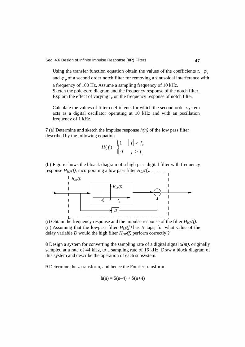
7 (a) Determine and sketch the impulse response h(n) of the low pass filter described by the following equation
H ff f
f fc
c
( ) =<
≥
⎧⎨⎪
⎩⎪
1
0
(b) Figure shows the bloack diagram of a high pass digital filter with frequency response HHP(f), incorporating a low pass filter HLP(f).
-fc-fc
D
HLP(f)
fc
HHP(f)
(i) Obtain the frequency response and the impulse response of the filter HHP(f). (ii) Assuming that the lowpass filter HLP(f) has N taps, for what value of the delay variable D would the high filter HHP(f) perform correctly ? 8 Design a system for converting the sampling rate of a digital signal x(m), originally sampled at a rate of 44 kHz, to a sampling rate of 16 kHz. Draw a block diagram of this system and describe the operation of each subsystem. 9 Determine the z-transform, and hence the Fourier transform
h(n) = δ(n–4) + δ(n+4)

48 Chapter 5 Digital Filters
Suggest a use for a filter with h(n) as its impulse response.
H z z z( ) = +− +4 4 What modification of the equation for h(n) is necessary before it can be used as the impulse response of a causal filter. 10 (a) Describe in details the window design techniques for the design of a finite impulse response (FIR) low pass filter with the frequency response specification as shown in figure (). Obtain and sketch the impulse response of this filter. Explain the main effects of varying the filter order.
X (f)
ffc-fc Using the window design technique and the filter impulse response from part (a) above, design a bank of digital filters for a telephony speech application to split a total bandwidth of 4 kHz to four equal width subbands.
(i) Write the cutoff frequencies and the equations for the response of the filter in each band. Your equations should include the numerical parameters needed to achieve the required cutoff frequencies. (ii) Choose a value for the number of taps of the filter in each band and explain
how the number of filter coefficients affects the filter response. (iii) Suggest an application for this filter bank. 11 Determine the values of a1 and a2 for which the second order system shown in the figure and operating at a sampling rate of 40 kHz becomes a sinusoidal oscillator with an oscillation frequency of 5 kHz. Plot a pole-zero diagram for the oscillator.

Sec. 4.6 Design of Infinite Impulse Response (IIR) Filters 49
z-1
z-1
-a 1
-a 2
Input x(n)Output y(n)
12 State the factors that affect the choice of a filter. The Z transfer function of a finite impulse response filter H(z) is given by
( )( )H z z z z z( ) . .= − + − +− − − −1 0 5 0 25 1 2 41 2 1 2 Obtain the equation for H(ω) the frequency response of this filter. Prove that H(ω) is a linear phase filter . Obtain the zeros of this filter and plot the pole-zero diagram for this filter.
13 Consider a second order infinite impulse response (IIR) system operating at a sampling rate of 40 KHz and with the z-transfer function given as
H z Gr z r zr z r z
( )( cos )
cos=
+ +
+ +
− −
− −
1 21 2
1 11 2 2
2 21 2 2
2
2
θθ
Assume that this system has a complex conjugate pair of poles and zeros. Rewrite the transfer function in terms of radii and the resonance angular frequencies of the poles and the zeros of the filter. Find the poles and the zeros for which the transfer function has a notch frequency response at a frequency of 10 kHz, and unit response at 0 Hz and 20 kHz. Obtain the frequency spectrum and write the difference equation of the filter. Plot its pole-zero diagram, and sketch its spectrum. 14 State the main effects of (i) a complex conjugate pair of poles, and (ii) a complex conjugate pair of zeros, on the frequency response of a filter. Using the window design method, derive an expression for the impulse response of a

50 Chapter 5 Digital Filters
causal lowpass digital finite impulse response (FIR) filter of length N operating at a sampling rate of 20 kHz and with a cutoff frequency of 5 kHz. State the effect of varying N on the frequency response of the filter. State what values of N are typically used in the design of a lowpass FIR filter. 15 Consider a second order all zero infinite impulse response (IIR) system operating at 20 KHz and with the z-transfer function given as
H zG
b z b z( ) =
+ +− −1 11
22
Assume that this system has a complex conjugate pair of poles. Rewrite the transfer function in terms of pole radius and pole resonance frequency. Find the values of the coefficients b1, b2 and the gain G for which this filter has a resonance frequency of 5 kHz, a gain G of unity at this frequency, and a bandwidth of 100 Hz. Plot its pole-zero diagram, and write its frequency response equation. Write the difference equation of this system.