Digital Controls & Digital Filters Lectures 13 & 14 13-14.pdf · Modi ed z-Transform Sampling Continuous-Time State-Space Model Closed-Loop Systems Sampling Of A Continuous-Time State

Modified z-Transform Sampling Continuous-Time State-Space Model Closed-Loop Systems

Digital Controls & Digital FiltersLectures 13 & 14

M.R. Azimi, Professor

Department of Electrical and Computer EngineeringColorado State University

Spring 2017

M.R. Azimi Digital Control & Digital Filters


Systems with Actual Time Delays-Application 2

Case 1: Delay in the Plant

Let t0 = kT + ∆T , K ∈ I, 0 < ∆ ≤ 1

C(s) = G(s)e−t0sE∗(s)

C(z) = Z [G(s)e−t0s]E(z) = Z[G(s)e−kTse−∆Ts

]E(z) =

z−kZ[G(s)e−∆Ts

]|∆=1−mE(z) = z−kZm [G(s)]E(z)

Thus, for this case we have

C(z) = z−kG(z,m)E(z)



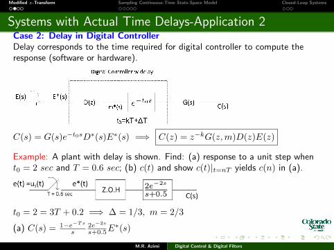
Systems with Actual Time Delays-Application 2Case 2: Delay in Digital ControllerDelay corresponds to the time required for digital controller to compute theresponse (software or hardware).

C(s) = G(s)e−t0sD∗(s)E∗(s) =⇒ C(z) = z−kG(z,m)D(z)E(z)

Example: A plant with delay is shown. Find: (a) response to a unit step whent0 = 2 sec and T = 0.6 sec; (b) c(t) and show c(t)|t=nT yields c(n) in (a).

t0 = 2 = 3T + 0.2 =⇒ ∆ = 1/3, m = 2/3

(a) C(s) = 1−e−Ts

s2e−2s

s+0.5E∗(s)



Systems with Actual Time Delays-Cont.

C(z) = (1− z−1)Z[

2e−2s

s(s+0.5)

]E(z) = (1− z−1)z−3Z

[2e−

T3

s

s(s+0.5)

]zz−1

C(z) = z−3Z[

2e−(1−2/3)Ts

s(s+0.5)

]= z−3Zm

[2

s(s+0.5)

] ∣∣∣m=2/3

= (0.7256z−0.3112)z3(z−1)(z−0.7408)

Expand C(z)z = (0.7256z−0.3112)

z4(z−1)(z−0.7408) and take IZT,

c(n) = [4− 3.27(0.7408)n−4]us(n− 4)

(b) Using shifting property C(s) = 2e−2s

s(s+0.5) =⇒ c(t) = L−1{ 2s(s+0.5)}|t=t−2

But 2s(s+0.5) = 4

s −4

s+0.5

Hence c(t) = 4(1− e−0.5(t−2))us(t− 2)

Now, c(n) = 4(1− e−0.5(t−2))us(t− 2)|t=nT = 4(1− e1e−0.5nT )us(nT − 2)

= (4− 4e1e−1.2e−0.5(n−4))us(n− 4) = [4− 3.27(0.7408)n−4]us(n− 4)



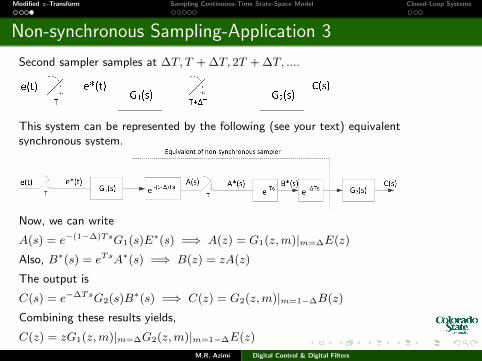
Non-synchronous Sampling-Application 3

Second sampler samples at ∆T, T + ∆T, 2T + ∆T, ....

This system can be represented by the following (see your text) equivalentsynchronous system.

Now, we can write

A(s) = e−(1−∆)TsG1(s)E∗(s) =⇒ A(z) = G1(z,m)|m=∆E(z)

Also, B∗(s) = eTsA∗(s) =⇒ B(z) = zA(z)

The output is

C(s) = e−∆TsG2(s)B∗(s) =⇒ C(z) = G2(z,m)|m=1−∆B(z)

Combining these results yields,

C(z) = zG1(z,m)|m=∆G2(z,m)|m=1−∆E(z)



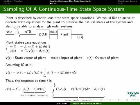
Sampling Of A Continuous-Time State Space System

Plant is described by continuous-time state-space equations. We would like to arrive atdiscrete state equations for the plant to preserve the natural states of the system andalso to be able to analyse high order systems.

Plant state-space equations,{v(t) = Acv(t) +Bcm(t)c(t) = Ccv(t) + dcm(t)

v(t) : State vector of plant m(t) : Input of plant c(t): Output of plant

Assuming IC at t0,

v(t) = φc(t− t0)v(t0) +t

t0

φc(t− τ)Bcm(τ)dτ

Thus, the response at time t is,

c(t) = Cc φc(t− t0)v(t0)︸︷︷︸zero−input response

+

tˆ

t0

Ccφc(t− τ)Bcm(τ)dτ + dcm(t)

︸︷︷︸zero−state response




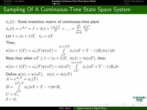
φc(t) : State transition matrix of continuous-time plant

φc(t) = eAct = I +Act+ (Act)2

2! + . . . =∞∑k=0

Akc t

k

k!

Let t = (n+ 1)T, t0 = nT

Then,

v((n+ 1)T ) = φc(T )v(nT ) +(n+1)TńT

φc(nT + T − τ)Bcm(τ)dτ

Note that when nT ≤ t < (n+ 1)T, m(t) = m(nT ), then:

v((n+ 1)T ) = φc(T )v(nT ) + m(nT )(n+1)TńT

φc(nT + T − τ)Bcdτ

Define x(n) = v(nT ), u(n) = m(nT )A = eAcT = φc(T )

B =nT+TńT

φc(nT + T − τ)dτBc

C = Ccd = dc




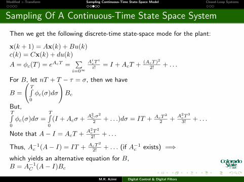
Then we get the following discrete-time state-space mode for the plant:

x(k + 1) = Ax(k) +Bu(k)c(k) = Cx(k) + du(k)

A = φc(T ) = eAcT =∑i=0∞

AicT

i

i! = I +AcT + (AcT )2

2! + . . .

For B, let nT + T − τ = σ, then we have

B =

(T

0

φc(σ)dσ

)Bc

But,T

0

φc(σ)dσ =T

0

(I +Acσ +A2

Cσ2

2 + . . .)dσ = IT + AcT2

2 +A2

cT3

3! + . . .

Note that A− I = AcT +A2

cT2

2! + . . .

Thus, A−1c (A− I) = IT + AcT

2

2! + . . . (if A−1c exists) =⇒

which yields an alternative equation for B,B = A−1

C (A− I)Bc




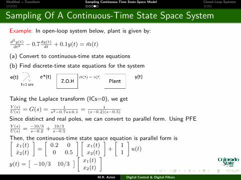
Example: In open-loop system below, plant is given by:

d2y(t)

dt2− 0.7 dy(t)

dt+ 0.1y(t) = m(t)

(a) Convert to continuous-time state equations

(b) Find discrete-time state equations for the system

Taking the Laplace transform (ICs=0), we get

Y (s)U(s)

= G(s) = 1s2−0.7s+0.1

= 1(s−0.2)(s−0.5)

Since distinct and real poles, we can convert to parallel form. Using PFEY (s)U(s)

= −10/3s−0.2

+ 10/3s−0.5

Then, the continuous-time state space equation is parallel form is[x1(t)x2(t)

]=

[0.2 00 0.5

] [x1(t)x2(t)

]+

[11

]u(t)

y(t) =[−10/3 10/3

] [ x1(t)x2(t)

]M.R. Azimi Digital Control & Digital Filters



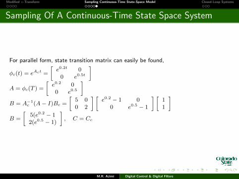
For parallel form, state transition matrix can easily be found,

φc(t) = eAct =

[e0.2t 0

0 e0.5t

]A = φc(T ) =

[e0.2 00 e0.5

]B = A−1

c (A− I)Bc =

[5 00 2

] [e0.2 − 1 0

0 e0.5 − 1

] [11

]B =

[5(e0.2 − 12(e0.5 − 1)

], C = Cc



Closed-Loop Systems

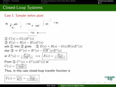
Case 1: Sampler before plant

1© C(s) = G(s)E∗(s)2© E(s) = R(s)−H(s)C(s)

sub 1© into 2© gives 3© E(s) = R(s)−G(s)H(s)E∗(s)

star 3© ⇒ E∗(s) = R∗(s)−GH∗(s)E∗(s)or E∗(s) = R∗(s)

1+GH∗(s)

=⇒ E(z) = R(z)

1+GH(z)

From 1© C∗(s) = G∗(s)E∗(s) or

C(z) = G(z)R(z)

1+GH(z)

Thus, in this case closed-loop transfer function is

T (z) = C(z)R(z) = G(z)

1+GH(z)



Closed-Loop Systems-Cont.

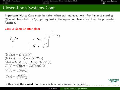
Important Note: Care must be taken when starring equations. For instance starring2© would have led to C(s) getting lost in the operation, hence no closed loop transfer

function.

Case 2: Sampler after plant

1© C(s) = G(s)E(s)2© E(s) = R(s)−H(s)C∗(s)C(s) = G(s)R(s)−G(s)H(s)C∗(s)C∗(s) = GR(s)−GH∗

(s)C∗(s)

C∗(s) = GR∗(s)

1+GH∗(s)

C(z) = GR(z)

1+GH(z)

In this case the closed loop transfer function cannon be defined.



Closed-Loop Systems-Cont.

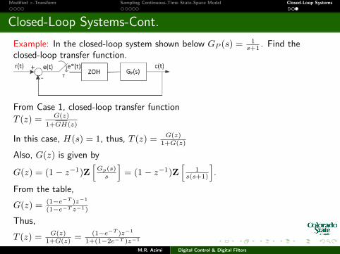
Example: In the closed-loop system shown below GP (s) = 1s+1 . Find the

closed-loop transfer function.

From Case 1, closed-loop transfer function

T (z) = G(z)

1+GH(z)

In this case, H(s) = 1, thus, T (z) = G(z)1+G(z)

Also, G(z) is given by

G(z) = (1− z−1)Z[Gp(s)s

]= (1− z−1)Z

[1

s(s+1)

].

From the table,

G(z) = (1−e−T )z−1

(1−e−T z−1)

Thus,

T (z) = G(z)1+G(z) = (1−e−T )z−1

1+(1−2e−T )z−1


Documents

Digital Controls & Digital Filters Lectures 13 & 14 13-14.pdf · Modi ed z-Transform Sampling Continuous-Time State-Space Model Closed-Loop Systems Sampling Of A Continuous-Time State