Digital compensation of distortion in audio systems318711/FULLTEXT01.pdf · Digital compensation of distortion in audio ... 5.9.1 Limitation of a sinusoid ... Investigate how a too

Institutionen för systemteknikDepartment of Electrical Engineering

Examensarbete

Digital compensation of distortion in audio systems

Examensarbete utfört i elektroniksystemvid Tekniska högskolan i Linköping

av

Fredrik Bengtsson, Rikard Berglund

LiTH-ISY-EX--10/4367--SE

Linköping 2010

Department of Electrical Engineering Linköpings tekniska högskolaLinköpings universitet Linköpings universitetSE-581 83 Linköping, Sweden 581 83 Linköping


Examensarbete utfört i elektroniksystem

vid Tekniska högskolan i Linköpingav

Fredrik Bengtsson, Rikard Berglund


Handledare: Kent Palmkvistisy, Linköpings universitet

Pär Gunnars RisbergActiwave AB

Examinator: Kent Palmkvistisy, Linköpings universitet

Linköping, 6 May, 2010

Avdelning, Institution

Division, Department

ElektroniksystemDepartment of Electrical EngineeringLinköpings universitetSE-581 83 Linköping, Sweden

Datum

Date

2010-05-06

Språk

Language

Svenska/Swedish

Engelska/English

Rapporttyp

Report category

Licentiatavhandling

Examensarbete

C-uppsats

D-uppsats

Övrig rapport

URL för elektronisk version

http://www.es.isy.liu.se

http://www.ep.liu.se

ISBN

—

ISRN


Serietitel och serienummer

Title of series, numberingISSN

—

Titel

TitleDigital kompensering av distorsion i ljudsystem


Författare

AuthorFredrik Bengtsson, Rikard Berglund

Sammanfattning

Abstract

The advancements of computational power in low cost FPGAs are giving the op-portunity to implement real-time compensation of loudspeakers and audio systems.The need for expensive commercial audio systems is reduced when the fidelity ofmuch cheaper audio systems easily can be improved by real-time compensation.The topic of this thesis is to investigate and evaluate methods for digital com-pensation of distortion in audio systems. More specifically, a VHDL module isimplemented to, when necessary, alleviate the problem of drastically deterioratingfidelity of the bass appearing when the input power is too high.

Nyckelord

Keywords Distortion, Digital Compensation, Signal Processing, Digital Filters, Audio Sys-tems, Amplifiers, Modelling, Audio Compressor, Audio Limiter

Abstract

The advancements of computational power in low cost FPGAs are giving the op-portunity to implement real-time compensation of loudspeakers and audio systems.The need for expensive commercial audio systems is reduced when the fidelity ofmuch cheaper audio systems easily can be improved by real-time compensation.The topic of this thesis is to investigate and evaluate methods for digital com-pensation of distortion in audio systems. More specifically, a VHDL module isimplemented to, when necessary, alleviate the problem of drastically deterioratingfidelity of the bass appearing when the input power is too high.

v

Acknowledgments

We would like to thank:Kent PalmkvistPär Gunnars RisbergEveryone at Actiwave ABSebastian AbrahamssonMarkus Råbefor their help in this thesis.

Fredrik Bengtsson and Rikard Berglund

vii

Contents

1 Background 11.1 Introduction . . . . . . . . . . . . . . . . . . . . . . . . . . . . . . . 11.2 Purpose . . . . . . . . . . . . . . . . . . . . . . . . . . . . . . . . . 11.3 Goals . . . . . . . . . . . . . . . . . . . . . . . . . . . . . . . . . . 21.4 Outline of the report . . . . . . . . . . . . . . . . . . . . . . . . . . 21.5 Denotations and definitions . . . . . . . . . . . . . . . . . . . . . . 3

2 Related theory and research 52.1 Energy and power . . . . . . . . . . . . . . . . . . . . . . . . . . . 5

2.1.1 Average pseudo power . . . . . . . . . . . . . . . . . . . . . 52.1.2 Root mean square . . . . . . . . . . . . . . . . . . . . . . . 5

2.2 Distortion . . . . . . . . . . . . . . . . . . . . . . . . . . . . . . . . 62.2.1 Undersampling . . . . . . . . . . . . . . . . . . . . . . . . . 62.2.2 Total harmonic distortion . . . . . . . . . . . . . . . . . . . 62.2.3 Modulation distortion . . . . . . . . . . . . . . . . . . . . . 62.2.4 IMD vs. THD . . . . . . . . . . . . . . . . . . . . . . . . . 7

2.3 Non-linearities in audio systems . . . . . . . . . . . . . . . . . . . . 72.3.1 Amplifier . . . . . . . . . . . . . . . . . . . . . . . . . . . . 72.3.2 Loudspeakers . . . . . . . . . . . . . . . . . . . . . . . . . . 7

2.4 Filters . . . . . . . . . . . . . . . . . . . . . . . . . . . . . . . . . . 82.4.1 Analog filters . . . . . . . . . . . . . . . . . . . . . . . . . . 82.4.2 Digital filters . . . . . . . . . . . . . . . . . . . . . . . . . . 82.4.3 IIR filters . . . . . . . . . . . . . . . . . . . . . . . . . . . . 92.4.4 FIR filters . . . . . . . . . . . . . . . . . . . . . . . . . . . . 10

2.5 Class-D amplifiers . . . . . . . . . . . . . . . . . . . . . . . . . . . 112.6 Audio compressor . . . . . . . . . . . . . . . . . . . . . . . . . . . . 11

2.6.1 Functionality . . . . . . . . . . . . . . . . . . . . . . . . . . 112.6.2 Limiter . . . . . . . . . . . . . . . . . . . . . . . . . . . . . 13

3 Test equipment 153.1 Loudspeaker A . . . . . . . . . . . . . . . . . . . . . . . . . . . . . 153.2 Amplifiers . . . . . . . . . . . . . . . . . . . . . . . . . . . . . . . . 16

3.2.1 Amplifier A . . . . . . . . . . . . . . . . . . . . . . . . . . . 163.2.2 Amplifier B . . . . . . . . . . . . . . . . . . . . . . . . . . . 17

ix

x Contents

3.2.3 Amplifier C . . . . . . . . . . . . . . . . . . . . . . . . . . . 183.3 Sound card . . . . . . . . . . . . . . . . . . . . . . . . . . . . . . . 183.4 Microphone . . . . . . . . . . . . . . . . . . . . . . . . . . . . . . . 193.5 Digital oscilloscope . . . . . . . . . . . . . . . . . . . . . . . . . . . 19

4 Investigation 21

4.1 Analysis of audio sequences . . . . . . . . . . . . . . . . . . . . . . 214.2 Identifying the cause of distortion . . . . . . . . . . . . . . . . . . . 224.3 Model of clipping . . . . . . . . . . . . . . . . . . . . . . . . . . . . 23

4.3.1 One tone test . . . . . . . . . . . . . . . . . . . . . . . . . . 234.3.2 Two tone test . . . . . . . . . . . . . . . . . . . . . . . . . . 274.3.3 Conclusion . . . . . . . . . . . . . . . . . . . . . . . . . . . 28

4.4 Saturation of amplifiers . . . . . . . . . . . . . . . . . . . . . . . . 284.4.1 Voltage saturation . . . . . . . . . . . . . . . . . . . . . . . 284.4.2 Over-current protection . . . . . . . . . . . . . . . . . . . . 28

4.5 Voltage saturation/frequency dependency . . . . . . . . . . . . . . 284.5.1 Bass/midrange driver test . . . . . . . . . . . . . . . . . . . 294.5.2 Full range loudspeaker test . . . . . . . . . . . . . . . . . . 30

4.6 Conclusion . . . . . . . . . . . . . . . . . . . . . . . . . . . . . . . 31

5 The proposed solution 33

5.1 Basic functionality of the model . . . . . . . . . . . . . . . . . . . . 335.2 Essential structure of the limiter . . . . . . . . . . . . . . . . . . . 34

5.2.1 LP prefiltering . . . . . . . . . . . . . . . . . . . . . . . . . 345.2.2 LP postfiltering . . . . . . . . . . . . . . . . . . . . . . . . . 345.2.3 Preserving a full frequency range signal . . . . . . . . . . . 34

5.3 Amplitude reduction of the bass channel . . . . . . . . . . . . . . . 345.3.1 Time multiplexing . . . . . . . . . . . . . . . . . . . . . . . 355.3.2 Scaling . . . . . . . . . . . . . . . . . . . . . . . . . . . . . 365.3.3 FFT and notch filter . . . . . . . . . . . . . . . . . . . . . . 385.3.4 Discussion and conclusions . . . . . . . . . . . . . . . . . . 38

5.4 Choice of filters . . . . . . . . . . . . . . . . . . . . . . . . . . . . . 395.4.1 Crossover . . . . . . . . . . . . . . . . . . . . . . . . . . . . 39

5.5 The decision making block . . . . . . . . . . . . . . . . . . . . . . . 405.5.1 The maximum block . . . . . . . . . . . . . . . . . . . . . . 415.5.2 Direct steering . . . . . . . . . . . . . . . . . . . . . . . . . 41

5.6 Optional functionality . . . . . . . . . . . . . . . . . . . . . . . . . 425.7 The volume control . . . . . . . . . . . . . . . . . . . . . . . . . . . 435.8 The complete limiter . . . . . . . . . . . . . . . . . . . . . . . . . . 445.9 Limiter simulations . . . . . . . . . . . . . . . . . . . . . . . . . . . 44

5.9.1 Limitation of a sinusoid with constant amplitude . . . . . . 455.9.2 Limitation of a ramping sinusoid . . . . . . . . . . . . . . . 465.9.3 Limitation of music . . . . . . . . . . . . . . . . . . . . . . 47

5.10 Conclusion . . . . . . . . . . . . . . . . . . . . . . . . . . . . . . . 47

Contents xi

6 VHDL implementation 496.1 FPGA . . . . . . . . . . . . . . . . . . . . . . . . . . . . . . . . . . 496.2 Clock domains . . . . . . . . . . . . . . . . . . . . . . . . . . . . . 496.3 Implementation and optimization . . . . . . . . . . . . . . . . . . . 50

6.3.1 Biquads . . . . . . . . . . . . . . . . . . . . . . . . . . . . . 506.3.2 Decision making block . . . . . . . . . . . . . . . . . . . . . 506.3.3 Miscellaneous . . . . . . . . . . . . . . . . . . . . . . . . . . 50

6.4 Volume control . . . . . . . . . . . . . . . . . . . . . . . . . . . . . 51

7 THD measurements 537.1 Introduction to THD measurements . . . . . . . . . . . . . . . . . 537.2 THD measurement . . . . . . . . . . . . . . . . . . . . . . . . . . . 53

7.2.1 Data collection . . . . . . . . . . . . . . . . . . . . . . . . . 547.3 Results . . . . . . . . . . . . . . . . . . . . . . . . . . . . . . . . . . 54

8 Conclusions and discussion 578.1 Audible improvement . . . . . . . . . . . . . . . . . . . . . . . . . . 578.2 Regarding the model . . . . . . . . . . . . . . . . . . . . . . . . . . 58

8.2.1 Functionality of the model . . . . . . . . . . . . . . . . . . . 588.2.2 Future work and discussion . . . . . . . . . . . . . . . . . . 58

8.3 Supplementary conclusion . . . . . . . . . . . . . . . . . . . . . . . 60

Bibliography 61

Chapter 1

Background

1.1 Introduction

The advancements of computational power in low cost FPGAs are giving the op-portunity to implement real-time compensation of loudspeakers and audio systems.The need for expensive commercial audio systems is reduced when the fidelity ofmuch cheaper audio systems easily can be improved by real-time compensation.Today it is possible to implement hardware that digitally compensates for e.g.phase delays, loudspeaker characteristics and distortion.

The topic of this master thesis is to investigate and evaluate methods for digitalcompensation of distortion in audio systems. It is well known that a lot moreenergy is needed to produce a loud bass sound than a loud high-pitched sound, i.e.,most of the sound energy in music comes from the kick drum and the bass guitaror bass synthesizer [16]. However, the limitations of amplifiers and loudspeakerswill result in drastically deteriorating fidelity when playing too loud, which is theproblem to be solved. Therefore, a hardware module, described in VHDL, will beimplemented in order to, when necessary, reduce the problem of arising distortion.

The area of interest is digital compensation of audio systems. The main ques-tions are: Is it possible to identify the cause of audible distortion due to too highvolume in the audio system and digitally compensate for this with a real-time com-pensating module in hardware? If yes, is this a reliable and flexible implementationthat is applicable in different audio systems?

The answers to these questions, among with others, will be presented in thismaster thesis.

1.2 Purpose

The purpose of this thesis is to gain further knowledge of the distortion renderedby too high input volume and how to compensate for this. The work was done atActiwave AB. There were four main tasks:

1

2 Background

1. Investigate how a too high input signal rendering audible distortion is digi-tally detected in an audio system.

2. Determine how the distortion can be compensated and develop a modelsolving the problem stated above.

3. Implement a VHDL module, similar to the earlier developed model, accord-ing to hardware limitations and processing time in a real-time hardwaresystem.

4. Present data comparing the distortion in the audio system when compensa-tion is on and off.

1.3 Goals

The main goals are to develop a fully working model in Scilab or Simulink andimplement the same model in hardware via VHDL. The model should compensatefor a too high input volume by performing calculations on a sound sequence. Thesignal should only be altered when necessary, i.e., when it is identified that thebass will give rise to distortion at a given volume. This allows the user to playmusic at a higher volume without getting the feeling that the audio system losesits high fidelity.

Further, the VHDL module might have differences compared to the previouslydeveloped model because of hardware restrictions that may arise. The VHDLmodule should be applicable in any Actiwave audio system. It has to be fairlyeasy to adapt to systems with different amplifiers and loudspeakers.

If different methods for any task are viable to implement in the module, theyshould be investigated as far as possible in the given time frame. A performancecomparison should be performed after implementation and a discussion shouldclearly motivate the choice of a specific model.

1.4 Outline of the report

Chapter 1 is an introduction to the thesis where background, purpose, goals,outline of the report and used denotations and definitions are stated.Chapter 2 briefly presents related research that the reader should be well ac-quainted with in order to fully understand this thesis.Chapter 3 lists all the test equipment used in this thesis and states their mostsignificant properties.Chapter 4 covers an investigation of how the audible distortion can be detectedand what its effects are.Chapter 5 covers the development of the proposed model and briefly discussesdifferent methods of solving the problem.Chapter 6 briefly covers the implementation of the VHDL described hardwaremodule on an FPGA.Chapter 7 presents the results achieved with the implemented VHDL module.

1.5 Denotations and definitions 3

Chapter 8 presents the conclusions of both the hardware and software model anddiscusses further development of the proposed solution.

1.5 Denotations and definitions

Software, abbreviations and acronyms used in this thesis are explained in thissection.

Scilabr

Scilab is an interactive platform for numerical computation providing a powerfulcomputing environment for engineering and scientific applications [4].

Simulinkr

Simulink is an environment for multidomain simulation and Model-Based Designfor dynamic and embedded systems. It provides an interactive graphical envi-ronment and a customizable set of block libraries that let you design, simulate,implement, and test a variety of time-varying systems, including communications,controls, signal processing, video processing, and image processing [23].

ISErWebPACKTM

ISE WebPACK design software is a fully featured front-to-back FPGA designsolution. ISE WebPACK is a tool for FPGA and CPLD design offering HDLsynthesis and simulation, implementation, device fitting, and JTAG programming[25].

ARTA

A program for the impulse response measurement and for real-time spectrum anal-ysis and frequency response measurements [8].

4 Background

Abbreviations and acronyms

Abbreviations and acronyms used in this report are stated below.

Acronyms Explanation

clk ClockDC Direct currentDSP Digital signal processorf FrequencyFFT Fast Fourier transformFIR Finite impulse responseFPGA Field programmable gate arrayf0 Bandwidthfc 3 dB cutoff frequencyfs Sampling frequencyFSM Finite-state machineHDL Hardware description languageHP High passIC Integrated circuitICP Injection-molded co-polymer polypropyleneIIR Infinite impulse responseIMD Intermodulation distortionIP Intellectual PropertyLC Inductor and capacitorLP Low passLR Linkwitz-RileyLSI Linear and shift-invariantLSB Least significant bitNS Noise shapingOP-amp Operational amplifierPCB Printed circuit boardPWM Pulse-width modulationQ QuantizationRMS Root mean squareS/PDIF Sony/Philips Digital Interconnect FormatSR Slew rateT PeriodTHD Total harmonic distortionTHD+N THD and noiseTOSLink Toshiba linkVHDL VHSIC HDLVHSIC Very High Speed ICVLSI Very Large Scale Integration

Chapter 2

Related theory and research

Related theory and research necessary to understand the thesis will be presentedin this chapter. However, the reader is expected to have relevant knowledge inmathematics and electronics.

2.1 Energy and power

Relevant energy and power definitions are stated below.

2.1.1 Average pseudo power

The average pseudo power for a non-periodic sequence x(n), with sample indexesN , is dimensionless and is defined in equation 2.1 [7]. Pseudo will be left out whentalking about the power.

P =1

2N + 1

N∑

n=−N

|x(n)|2 (2.1)

The power P of a time continuous and periodic signal with the period T isdefined in equation 2.2 [21].

P =1

T

∫

T

|x(t)|2dt (2.2)

2.1.2 Root mean square

The root mean square (RMS) is defined as in equation 2.3 if x(n) is a periodicsequence with period N [21].

VRMS =

√

√

√

√

1

N

N−1∑

n=0

|x(n)|2 (2.3)

5

6 Related theory and research

2.2 Distortion

This section describes the relevant types of distortion and why they occur.

2.2.1 Undersampling

Undersampling distortion occurs when the sampling frequency isn’t high enoughto ensure that the reconstructed signal is not too far from the original one. Toensure this, the sampling theorem has to be fulfilled [7].

Sampling theorem (The Nyquist Sampling Theorem)If a continuous time signal xa(t) is band limited to ω = ω0 (f = f0), i.e.,

Xa(jω) = 0, |ω| > ω0 = 2πf0

then xa(t) can be recovered from the samples x(n) = xa(nT ) provided that

fs = 1Ts

> 2f0.

However, the input signal to the audio systems used in this thesis are alreadydigital with a given sampling frequency of 44.1 kHz. Distortion caused by under-sampling will therefore not be further discussed in this thesis.

2.2.2 Total harmonic distortion

Consider the fundamental sinusoid, X1sin(ω1t + φ1). The harmonics are definedas sinusoids with an arbitrary amplitude Xk and phase φk, where the frequencyis ωk = kω1, where k = 2, 3, ... [21]. The harmonics are simply a multiple of afrequency existing in the input signal.

Total harmonic distortion (THD) is a measurement of the amount of harmonicsin a non-sinusoid shaped signal. THD is the ratio between the harmonics RMSand the complete signals RMS. The DC-component is assumed to be zero. Thedefinition follows in equation 2.4. k is the number of the harmonic where k = 1 isthe fundamental and e denotes the RMS of the sinusoids [21].

T HD =

√

∑∞k=2 X2

ke√

∑∞k=1 X2

ke

(2.4)

Equation 2.5 defines an alternative definition of THD.

T HD =

√

∑∞k=2 X2

ke

X1e

(2.5)

2.2.3 Modulation distortion

Modulation distortion, or sometimes called intermodulation distortion (IMD), isall frequencies not harmonically related to the input signal in the loudspeakersoutput. Noise is however not IMD [10]. Consider two frequencies, f1 and f2, where

2.3 Non-linearities in audio systems 7

f2 is the highest, in the input signal. The non-linearities will create the differencesand sums of the input frequencies, hence, f1 +f2 and f2 −f1. Unfortunately, sincethere are harmonics, even more IMD frequencies will appear from all possiblecombinations of frequencies [13].

2.2.4 IMD vs. THD

IMD is almost always greater in magnitude compared to THD. Most consider thistype of distortion to be by far more offensive because, unlike THD, the frequenciesappearing are not harmonics related to the fundamental and are therefore morelikely to be described as irritating to the listener [10].

2.3 Non-linearities in audio systems

This section will describe the most important non-linearities occurring in audiosystems.

2.3.1 Amplifier

A few of the most common causes of a distorted waveform is specified below. Ingeneral, electronics produce far less distortion than the loudspeaker itself [19].

SaturationThe output voltage is limited to a minimum and maximum value close to the powersupply voltages. Saturation occurs when the amplifiers voltage gain produces anoutput that is greater or less than the maximum or minimum voltage respectively[24]. A signal is referred to as clipped when the maximum or minimum voltage issaturated.

Slew rateThe amplifier has a maximum rate of voltage change which is referred to as slewrate (usually defined as volts/ms). The output waveform will be distorted whenthe slew rate is reached.

Non-linear transfer functionNo electrical components are ideal. Therefore some non-linearity will always beintroduced in amplifiers, causing a non-linear transfer function. The introducedTHD and noise is most often specified in the data sheets of a amplifier. However,IMD is not always stated in data sheets.

2.3.2 Loudspeakers

Ideally a loudspeaker would produce acoustic waves, which are a linear transfor-mation of the electrical input signal [17]. However, non-linearities exists and someof them, depending on loudspeaker type, are produced by:


The voice coilIn order to have a bass reproduction with high enough power, a large voice coilexcursion is required. This increases the already inherent non-linear distortion[17]. The non-linearities in a coil has it origin in the fact that they are not idealcomponents, i.e., they have both resistance and capacitance, but foremost, in thefact that the inductance of a coil can vary largely with the current [20].

The diaphragmFirst of all, the diaphragm does not work as one single unit. The acousto-mechanical impedance of the diaphragm varies over its area, ranging from beingclamped at the edges and relatively free to move in the middle. Low frequencydisplacement limits are generally set by the excursion capability of the diaphragmrelative to the fixed electrodes [9]. The frequency response is clearly affected bythe diaphragms properties causing a non-linear behavior.

The enclosureThe air spring provided by the sealed enclosure causes some non-linearity. Forhigh air volume displacements the restoring force of the enclosure can becomenon-linear; normally, for volumes changes no greater than about ±5 %, this non-linearity may be neglected [9].

2.4 Filters

The term filter can be explained as a mapping of an input signal to an outputsignal. The mapping can often be described with a mathematical expression.In this thesis, a filter will be defined as a frequency selective filter working withelectrical signals. A frequency selective filter has the property of rejecting specifiedfrequencies and letting others pass [11].

2.4.1 Analog filters

The input signal to an analog filter is often time continuous and the filter can eitherbe active or passive. The passive filter consists of components such as resistors,inductors and capacitors. Passive filters are important since they are often usedas reference when designing more advanced filters [21].

Active filters generally consists of resistors, capacitors and operational am-plifiers (OP-amps) [21]. Active filters were created to alleviate the non-wantedproperties of the inductors such as large physical size, weight and non-linearities.An active filter can opposed to passive filters generate signal energy, i.e. amplifythe signal, and if wrongly constructed they can therefore be unstable [11].

2.4.2 Digital filters

Digital filters are working with discrete-time signals and have become more andmore important in general, but also because it is more common to implementdigital signal processing today. Discrete-time filters are often designed with passive

2.4 Filters 9

time continuous filters as reference. Some characteristic properties of the digitalfilters are stated below [21].

Sensitivity: Digital systems are, compared to analog systems, independent ofcomponent properties such as manufacturing precision, aging and temperaturesensitivity. Digital systems are therefore less sensitive to component variationsand gives a higher reliability.

Physical properties: Using VLSI technology both shrinks the physical size andthe power consumption.

Flexibility: It is relatively easy to design a general DSP that can be used formany different purposes.

Quantization: All signals are quantized in digital systems. This may lead toproblems of different kinds.

2.4.3 IIR filters

The impulse response of an IIR filter can only be implemented recursively [21].The advantage with IIR filters is that they can be implemented with a lower orderthan FIR filters and still meet the same specifications [7]. However, IIR filtershave a non-linear phase response, but can still be made arbitrarily close to thelinear-phase response with increasing cost [12].

Digital bi-quadratic filters

The filter is often abbreviated biquad since the transfer function is a ratio of twoquadratic functions in the z-domain as seen in equation 2.6. The filter has a cutoffslope of 12 dB/octave, but a higher slope can be achieved by cascading filters,which is preferred instead of using a single 4th order design, since higher ordersresult in higher coefficient sensitivity [5].

H(z) =a0 + a1z−1 + a2z−2

1 + b1z−1 + b2z−2(2.6)

The most straightforward implementation is the direct form I, seen in differenceequation 2.7 and figure 2.1 [5].

y(n) = a0x(n) + a1x(n − 1) + a2x(n − 2) + b1y(n − 1) + b2y(n − 2) (2.7)

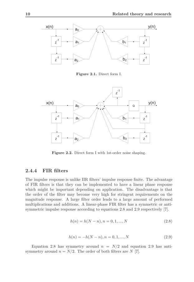
At low frequencies, biquads are more susceptible to quantization error, mainlyfrom the feedback coefficients b1 and b2, but also from the limited amount of bitsstored in the delay memory. Lack of resolution in the coefficients makes a precisepositioning of the poles difficult and the delay memory problem is inherited fromthe limited amount of bits that can be stored. One way of alleviating these issuesis to add the quantization error to the next sample calculation. This techniqueis called noise shaping (NS) and the 1st-order of NS is shown in figure 2.2 whereboth the output of the summation and the quantized output of the summation isfed back (compare with figure 2.1) [5].


Figure 2.1. Direct form I.

Figure 2.2. Direct form I with 1st-order noise shaping.

2.4.4 FIR filters

The impulse response is unlike IIR filters’ impulse response finite. The advantageof FIR filters is that they can be implemented to have a linear phase responsewhich might be important depending on application. The disadvantage is thatthe order of the filter may become very high for stringent requirements on themagnitude response. A large filter order leads to a large amount of performedmultiplications and additions. A linear-phase FIR filter has a symmetric or anti-symmetric impulse response according to equations 2.8 and 2.9 respectively [7].

h(n) = h(N − n), n = 0, 1, ..., N (2.8)

h(n) = −h(N − n), n = 0, 1, ..., N (2.9)

Equation 2.8 has symmetry around n = N/2 and equation 2.9 has anti-symmetry around n = N/2. The order of both filters are N [7].

2.5 Class-D amplifiers 11

2.5 Class-D amplifiers

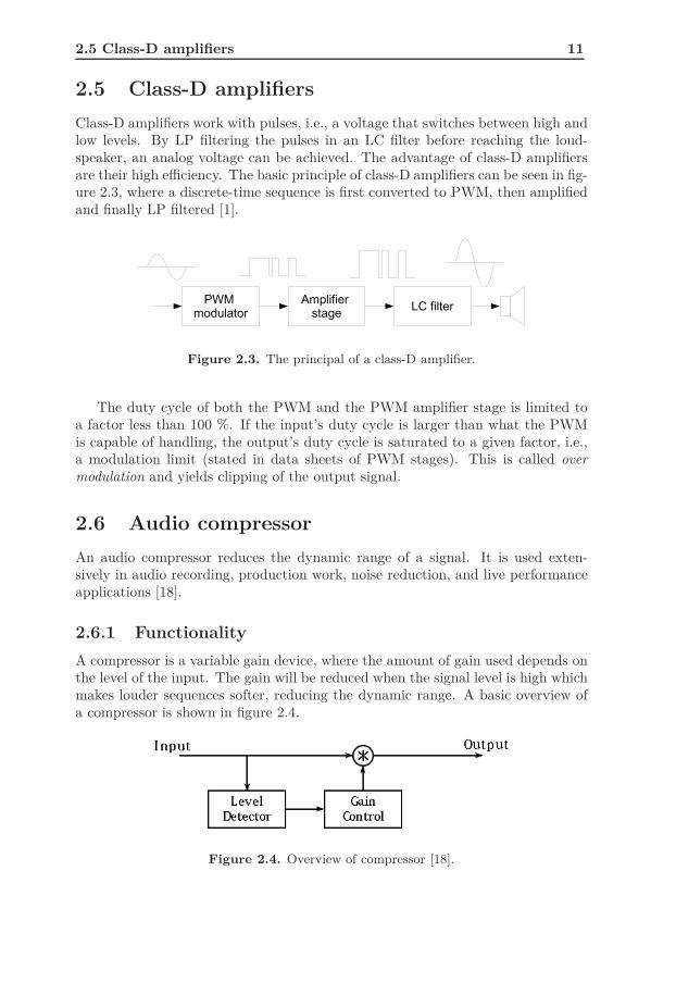
Class-D amplifiers work with pulses, i.e., a voltage that switches between high andlow levels. By LP filtering the pulses in an LC filter before reaching the loud-speaker, an analog voltage can be achieved. The advantage of class-D amplifiersare their high efficiency. The basic principle of class-D amplifiers can be seen in fig-ure 2.3, where a discrete-time sequence is first converted to PWM, then amplifiedand finally LP filtered [1].

Figure 2.3. The principal of a class-D amplifier.

The duty cycle of both the PWM and the PWM amplifier stage is limited toa factor less than 100 %. If the input’s duty cycle is larger than what the PWMis capable of handling, the output’s duty cycle is saturated to a given factor, i.e.,a modulation limit (stated in data sheets of PWM stages). This is called over

modulation and yields clipping of the output signal.

2.6 Audio compressor

An audio compressor reduces the dynamic range of a signal. It is used exten-sively in audio recording, production work, noise reduction, and live performanceapplications [18].

2.6.1 Functionality

A compressor is a variable gain device, where the amount of gain used depends onthe level of the input. The gain will be reduced when the signal level is high whichmakes louder sequences softer, reducing the dynamic range. A basic overview ofa compressor is shown in figure 2.4.

Figure 2.4. Overview of compressor [18].


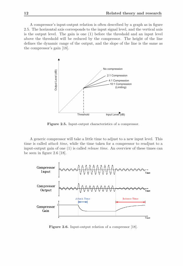
A compressor’s input-output relation is often described by a graph as in figure2.5. The horizontal axis corresponds to the input signal level, and the vertical axisis the output level. The gain is one (1) before the threshold and an input levelabove the threshold will be reduced by the compressor. The height of the linedefines the dynamic range of the output, and the slope of the line is the same asthe compressor’s gain [18].

Figure 2.5. Input-output characteristics of a compressor.

A generic compressor will take a little time to adjust to a new input level. Thistime is called attack time, while the time taken for a compressor to readjust to ainput-output gain of one (1) is called release time. An overview of these times canbe seen in figure 2.6 [18].

Figure 2.6. Input-output relation of a compressor [18].

2.6 Audio compressor 13

2.6.2 Limiter

A limiter is a compressor where the compression of the signal above a certainthreshold is very high, i.e., the output is limited to the specified threshold inde-pendent of the input signal level above the threshold. A limiter can also be definedas in figure 2.5, i.e., an input-output gain of at least 10:1 [18].

Chapter 3

Test equipment

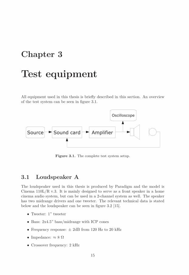
All equipment used in this thesis is briefly described in this section. An overviewof the test system can be seen in figure 3.1.

Figure 3.1. The complete test system setup.

3.1 Loudspeaker A

The loudspeaker used in this thesis is produced by Paradigm and the model isCinema 110L/R v.3. It is mainly designed to serve as a front speaker in a homecinema audio system, but can be used in a 2-channel system as well. The speakerhas two midrange drivers and one tweeter. The relevant technical data is statedbelow and the loudspeaker can be seen in figure 3.2 [15].

• Tweeter: 1” tweeter

• Bass: 2x4.5” bass/midrange with ICP cones

• Frequency response: ± 2dB from 120 Hz to 20 kHz

• Impedance: ≈ 8 Ω

• Crossover frequency: 2 kHz

15

16 Test equipment

• Enclosure: 2-way closed cabinet

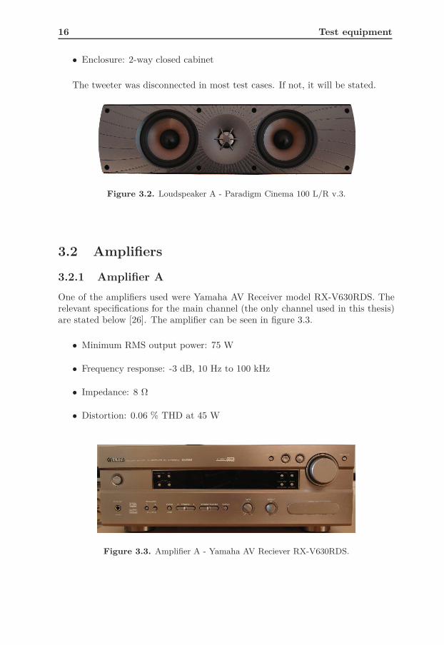
The tweeter was disconnected in most test cases. If not, it will be stated.

Figure 3.2. Loudspeaker A - Paradigm Cinema 100 L/R v.3.

3.2 Amplifiers

3.2.1 Amplifier A

One of the amplifiers used were Yamaha AV Receiver model RX-V630RDS. Therelevant specifications for the main channel (the only channel used in this thesis)are stated below [26]. The amplifier can be seen in figure 3.3.

• Minimum RMS output power: 75 W

• Frequency response: -3 dB, 10 Hz to 100 kHz

• Impedance: 8 Ω

• Distortion: 0.06 % THD at 45 W

Figure 3.3. Amplifier A - Yamaha AV Reciever RX-V630RDS.

3.2 Amplifiers 17

3.2.2 Amplifier B

The second amplifier used is an Actiwave designed class-D amplifier PCB withthe 20 W Stereo Digital Amplifier Power Stage TAS5602 from Texas Instrument.The PCBs are normally mounted inside the loudspeakers, but in the test setupused in this thesis the PCB will be placed outside the loudspeaker. The relevantspecifications of the output stage are stated below and the PCB can be seen infigure 3.4 [22].

• Continuous output power: 19 W at 24 V and 8 Ω

• Frequency response: -3 dB, 10 Hz to 100 kHz

• Impedance: 8 Ω

• Maximum output swing: < 24 V since Vdd = 24 V (not stated in data sheet)

• Distortion: 0.08 % THD at 10 W, 24 V, 1 kHz and 8 Ω

• Modulation limit: 97.7 %

• Sample frequency: 44.1 kHz

Figure 3.4. Amplifier B.

Figure 3.5 shows the data flow between digital sample and output. The outputfrom the DSP is modulated to PWM and then amplified by the power stage beforebeing subject to LP filtering.

Figure 3.5. Data flow of amplifier B.

18 Test equipment

3.2.3 Amplifier C

The third amplifier used is an Actiwave design as well. The specifications are thesame as in amplifier B, but the data flow is different as can be seen in figure 3.7.The DSP and the digital-to-PWM class-D controller has been replaced with anFPGA. The PCB can be seen in figure 3.6.

Figure 3.6. Amplifier C.

Figure 3.7. Data flow of amplifier C.

3.3 Sound card

The sound card used was an M-AUDIO Firewire 410 and can be seen in figure 3.8.The technical data relevant to what have been used in this thesis is stated below[14].

• Input: Analog (used for microphone)

• Output: S/PDIF on TOSLink optical connector

• Frequency response: 20-40 kHz ± 1 dB

• Distortion: 0.00281 % THD + N

3.4 Microphone 19

Figure 3.8. M-Audio Firewire 410 Sound card.

3.4 Microphone

The microphone used was a Behringer ECM8000. Further information regardingthe microphone is left out since it is not considered necessary.

3.5 Digital oscilloscope

The digital oscilloscope used was a UNI-T UT3062C. Further information regard-ing the digital oscilloscope will be left out since it is not considered necessary.

Chapter 4

Investigation

This chapter will present different investigations performed in order to identify thecause of audible distortion due to too high signal swing.

4.1 Analysis of audio sequences

Several audio sequences were played, recorded and analyzed with loudspeaker Aand amplifier A. One of these will be shown to illustrate the difficulty of recognizingsigns of distortion in an audio sequence. Figure 4.1(a) shows a short test sequence,referred to as sequence A, with two bass beats from the song Crazy by Lumidee.

Sequence A was played at a volume where distortion was clearly audible. Therecorded response can be seen in figure 4.1(b). The recording was made in asmall and echoic room sensitive to the rooms own impulse response. Studying thedifferences between the played and the recorded signals reveals a few things.

First of all, the recorded signal will always be different since both the room’sand the audio equipments’ impulse responses will affect the waveform.

Further, the envelope of the signals are similar, but the distortion adds higherfrequencies that can be seen as the faster swings up and down below the signalsenvelope. The origin of these higher frequencies will be explained in section 4.3.

Except the differences stated above, it is difficult to gain any useful informationby comparing played and recorded signals with clearly audible distortion.

The spectra of both the played and the recorded sequence A is not shown sinceit did not reveal anything of interest. In general, differences not seen in the timedomain could possibly be revealed in the frequency domain.

LP filtering sequences A reveals that most of the signal’s power is located in thelower frequency band. This can be seen in figure 4.2. A visual comparison of figure4.1(a) and 4.2 shows the strong resemblance even though higher frequencies arelacking. This result shows in what frequency band the signal’s energy is located,giving a starting point for the implementation of the compensating model.

21

22 Investigation

0 0.5 1 1.5 2 2.5 3 3.5 4

x 104

−1

−0.8

−0.6

−0.4

−0.2

0

0.2

0.4

0.6

0.8

1

(a) Sequence A played.

0 0.5 1 1.5 2 2.5 3 3.5 4

x 104

−1

−0.8

−0.6

−0.4

−0.2

0

0.2

0.4

0.6

0.8

1

(b) Sequence A recorded.

Figure 4.1. Comparison of the played and recorded sequence A.

4.2 Identifying the cause of distortion

Loudspeaker A and amplifier A was used for playback. The oscilloscope wasconnected at the input of the loudspeaker. By raising the volume, it was revealedthat the audible distortion coincided with the amplifier’s output voltage saturation,i.e., the signal was clipped. The distortion can be heard when the output swingis a few volts under maximum (before the signal is clipped) since the closer the

4.3 Model of clipping 23

0 0.5 1 1.5 2 2.5 3 3.5 4

x 104

−1

−0.8

−0.6

−0.4

−0.2

0

0.2

0.4

0.6

0.8

1

Figure 4.2. The LP filtered sequence A.

swing gets to the maximum, the more distortion was observed on the top and onthe bottom of the sinusoid.

By this test the conclusion is drawn that in this case the audible distortionprimarily has nothing to do with the loudspeakers inability to reproduce soundof high power, but with the amplifier’s inability to produce correct high powersignals to the loudspeaker.

Amplifier A was exchanged to amplifier B since the system to be used in thefinal product uses Actiwave’s own amplifier PCB (amplifier B or a similar PCB).One significant difference is that the Actiwave amplifier PCBs are class-D whileamplifier A is analog.

The same test, i.e., raising the volume and observing the oscilloscope, wasperformed with the same result for amplifier B as well.

4.3 Model of clipping

A Simulink model was created to analyze how the saturation of sinusoids affectthe spectrum. The effects of a clipped signal will be described in this section.

4.3.1 One tone test

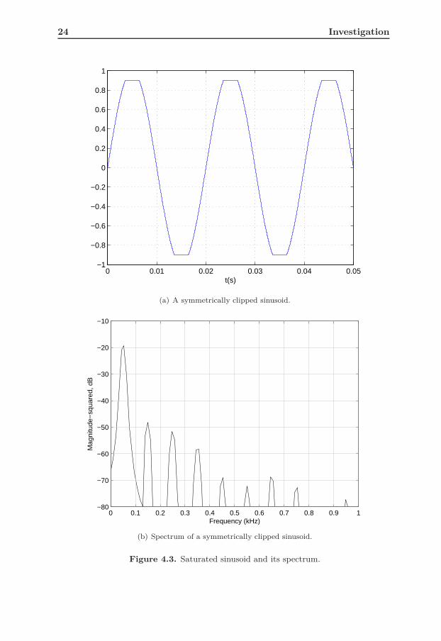
Three different kinds of saturations was investigated and they can, together withtheir spectra, be seen in figures 4.3, 4.4 and 4.5. How an input signal is saturated,e.g., if only the top, only the bottom, both top and bottom are clipped, and if theclip is symmetric or not, affects the magnitude of the distortion at the output andat what frequency the distortion mainly arises.

24 Investigation

0 0.01 0.02 0.03 0.04 0.05−1

−0.8

−0.6

−0.4

−0.2

0

0.2

0.4

0.6

0.8

1

t(s)

(a) A symmetrically clipped sinusoid.

0 0.1 0.2 0.3 0.4 0.5 0.6 0.7 0.8 0.9 1−80

−70

−60

−50

−40

−30

−20

−10

Frequency (kHz)

Mag

nitu

de−

squa

red,

dB

(b) Spectrum of a symmetrically clipped sinusoid.

Figure 4.3. Saturated sinusoid and its spectrum.


0 0.01 0.02 0.03 0.04 0.05−1

−0.8

−0.6

−0.4

−0.2

0

0.2

0.4

0.6

0.8

1

t(s)

(a) Asymmetrically clipped sinusoid.

0 0.1 0.2 0.3 0.4 0.5 0.6 0.7 0.8 0.9 1−80

−70

−60

−50

−40

−30

−20

−10

Frequency (kHz)

Mag

nitu

de−

squa

red,

dB

(b) Spectrum of an asymmetrically clipped sinusoid.


26 Investigation

0 0.01 0.02 0.03 0.04 0.05−1

−0.8

−0.6

−0.4

−0.2

0

0.2

0.4

0.6

0.8

1

t(s)

(a) Asymmetrically clipped sinusoid.

0 0.1 0.2 0.3 0.4 0.5 0.6 0.7 0.8 0.9 1−80

−70

−60

−50

−40

−30

−20

−10

Frequency (kHz)

Mag

nitu

de−

squa

red,

dB

(b) Spectrum of an asymmetrically clipped sinusoid.



4.3.2 Two tone test

The superposition of two frequencies are shown in figure 4.6(a) and its spectrumin figure 4.6(b). As seen in the figures, several input frequencies increases thecomplexity of the amount and magnitude of the upcoming distortion.

0.01 0.02 0.03 0.04 0.05 0.06 0.07 0.08 0.09−0.8

−0.6

−0.4

−0.2

0

0.2

0.4

0.6

0.8

t(s)

(a) Clipped signal.

0 50 100 150 200 250 300 350 400 450 500−80

−75

−70

−65

−60

−55

−50

−45

−40

−35

−30

Frequency (Hz)

Mag

nitu

de−

squa

red,

dB

(b) Spectrum of clipped signal.

Figure 4.6. A clipped signal consisting of f1 = 90 Hz and f2 = 100 Hz.

28 Investigation

4.3.3 Conclusion

As seen in figure 4.6(b), clipping produces THD and IMD at both higher and lowerfrequencies than the input frequencies, however, they have far less power. THDand IMD is also created by other non-linearities in the complete system.

The human ear has a dynamic range that goes from 0 dB at the threshold ofhearing to 120 dB at the threshold of pain (depending of frequency) [2]. Lookingat the simulation results, the magnitude of the unwanted frequencies are at least20 dB lower than the fundamental. There is apparently enough power in thedistortion for the human ear to hear it, presupposed that the fundamental toneis played at a high volume, which it must be in order to achieve clipping in theamplifier.

Double-blind subjective tests show that 3 % THD is audible on different typesof sounds. With carefully selected material (such as a flute solo) detecting THDdown to 2 % or 1 % might be possible. A THD of 1 % with sine waves is audible[6].

The conclusion is that, looking at a music sequence will not easily reveal anyof the effects of clipping since the amount of ingoing frequencies are too large, andto distinguish smaller changes in magnitude of these frequencies are very difficult.Distortion is however quite easily detected by the human ear and distortion, causedby clipping or not, should be kept to an absolute minimum to maintain high fidelity.

4.4 Saturation of amplifiers

The output of the amplifier can saturate either because the maximum output swingisn’t high enough to describe the signal or because the over-current protection isactivated.

4.4.1 Voltage saturation

The cause of saturation differs with the structure of the amplifier stage. A class-Aamplifier is limited by the maximum output voltage while a class-D amplifier canalso be limited by the modulation limit that clips the signal.

4.4.2 Over-current protection

The other case of saturation can be caused by the current limitations of the am-plifier. If the power of the output signal is too large, it will result in that Imax

is reached. The output voltage will then drop according to U = RImax, since thecurrent I is limited. Sinking too much current from the amplifier could also resultin a protective shut down of the amplifier circuit.

4.5 Voltage saturation/frequency dependency

The dependency between voltage saturation and frequency will be investigatedand described in this section.

4.5 Voltage saturation/frequency dependency 29

4.5.1 Bass/midrange driver test

Loudspeaker A and amplifier B was used for playback. By applying sine waves atdifferent frequencies and different volume, the maximum voltage for non-audibledistortion (V1) and the minimum voltage for audible distortion (V2) was notedwith the oscilloscope and stated in table 4.1. Multitone tests were performed aswell. Note that this data is measured while the tweeter was disconnected.

f V1 V2

50 21.5 22.890 22 22.8100 22 22.8110 20.8 23120 22 2350, 90 22.4 22.890, 100 22.4 2350, 120 22.4 23100, 120 21.6 22.850, 90, 120 21 22.890, 100, 120 22 22.820, 30, 35 21.6 22.420, 50, 120 22.4 22.835, 50, 65 22 22.825, 35, 40 22 22.425, 30, 35, 40, 45 22 22.420, 50, 60, 90, 120 22 22.830, 50, 100, 110, 120 21 22.8

Table 4.1. Voltages for output signal with and without distortion on bass/midrangedriver in loudspeaker A.

The accuracy of the oscilloscope is an error source, as well as the inability toadjust the volume with enough granularity, but judging by the data given in table4.1, there is an approximate maximum output voltage of 22 V in the frequencyband investigated. Ideally, if the granularity of the volume adjustment was better,V1 and V2 would be the same.

30 Investigation

4.5.2 Full range loudspeaker test

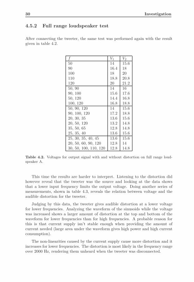
After connecting the tweeter, the same test was performed again with the resultgiven in table 4.2.

f V1 V2

50 14 15.690 16.4 18100 18 20110 18.8 20.8120 20 21.250, 90 14 1690, 100 15.6 17.650, 120 14.4 16.8100, 120 16.8 18.850, 90, 120 14 15.690, 100, 120 17.2 18.820, 30, 35 13.6 15.620, 50, 120 13.2 14.835, 50, 65 12.8 14.825, 35, 40 13.6 15.625, 30, 35, 40, 45 13.6 15.620, 50, 60, 90, 120 12.8 1430, 50, 100, 110, 120 12.8 14.8

Table 4.2. Voltages for output signal with and without distortion on full range loud-speaker A.

This time the results are harder to interpret. Listening to the distortion didhowever reveal that the tweeter was the source and looking at the data showsthat a lower input frequency limits the output voltage. Doing another series ofmeasurements, shown in table 4.3, reveals the relation between voltage and theaudible distortion for the tweeter.

Judging by this data, the tweeter gives audible distortion at a lower voltagefor lower frequencies. Analyzing the waveform of the sinusoids while the voltagewas increased shows a larger amount of distortion at the top and bottom of thewaveform for lower frequencies than for high frequencies. A probable reason forthis is that current supply isn’t stable enough when providing the amount ofcurrent needed (large area under the waveform gives high power and high currentconsumption).

The non-linearities caused by the current supply cause more distortion and itincreases for lower frequencies. The distortion is most likely in the frequency rangeover 2000 Hz, rendering them unheard when the tweeter was disconnected.

4.6 Conclusion 31

f V1 V2

20 11.6 13.225 12.4 1430 14 15.635 13.6 15.640 13.6 15.245 14 15.650 14 15.655 13.2 15.260 14.4 16.465 15.2 17.670 14.4 16.475 14.4 16.480 15.6 17.685 15.2 17.290 16.4 18100 18 20110 18.8 20.8120 20 21.2

Table 4.3. Voltages for output signal with and without distortion on full range loud-speaker A.

4.6 Conclusion

If there is no tweeter connected to the output channel and if the bass/midrangedriver is incapable of reproducing high frequencies, the solution for eliminatingdistortion is to limit the outgoing voltage to 22 V in order to ensure no clippingof the signal, i.e., limit the swing of the bass.

If the bass/midrange driver is capable of playing higher frequencies it is alsocapable of reproducing high frequency distortion. A detection of high power con-sumption (high RMS) could then be used to limit the bass. Another solutionwould be to simply lower the bass in the full range channels, i.e., the channel withelements capable of reproducing high frequencies, and let any other bass channelshave a higher output voltage allowed.

The work in this thesis is primarily focusing on eliminating the distortioncaused by the bass and occurring in the bass/midrange drivers. The distortion inthe tweeter will not be further investigated.

Chapter 5

The proposed solution

The proposed solution for ensuring the output to not get clipped will be explainedand discussed in this chapter. Several models have been developed in softwarein order to choose the model with the best functionality and the least hardwarerequirements. The modeling started in Scilab but later Simulink was used in orderto reduce the translation from Scilab code to VHDL.

Chapter 6 will describe the hardware implementation of the developed model.The choice of the model is made with the hardware implementation in mind inorder to create a VHDL module suitable for implementation in Actiwave’s existingsystem and its inherited requirements.

5.1 Basic functionality of the model

According to section 4.6 a maximum output voltage exists in order to not endup with a clipped signal. This voltage has to be matched to a maximum digitalsample value that never should be exceeded. The proposed solution is to use alimiter (audio compressor), as explained in section 2.6. The limiter will limit thedigital sample values, which makes it impossible to end up with a clipped analogsignal.

As earlier mentioned, most of the signal’s power is in the bass frequencies andthis thesis is focused on reducing distortion in the bass/midrange driver, henceonly the swing of lower frequencies has to be decreased in order to reduce thetotal amplitude sufficiently. The swing of the bass should only be altered whereit, according to real-time measurements, is estimated to affect the fidelity of theoutput, e.g., at loud bass beats. This will leave the bass intact during parts ofsound sequences where the bass gives the listener a perception of a full and naturalsound. By only applying the limiter at a low frequency band the higher frequenciesin a sound sequence will be unaffected. This is important since the total experienceof the sound should not be altered, but only improved when necessary.

33

34 The proposed solution

5.2 Essential structure of the limiter

Parts of the structure of the limiter are more or less necessary in order to achievehigh performance. These parts will be explained in this section. Dashed blockswithout content in the figures are to be defined later in the chapter.

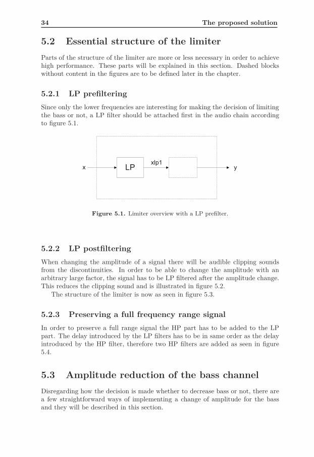
5.2.1 LP prefiltering

Since only the lower frequencies are interesting for making the decision of limitingthe bass or not, a LP filter should be attached first in the audio chain accordingto figure 5.1.

Figure 5.1. Limiter overview with a LP prefilter.

5.2.2 LP postfiltering

When changing the amplitude of a signal there will be audible clipping soundsfrom the discontinuities. In order to be able to change the amplitude with anarbitrary large factor, the signal has to be LP filtered after the amplitude change.This reduces the clipping sound and is illustrated in figure 5.2.

The structure of the limiter is now as seen in figure 5.3.

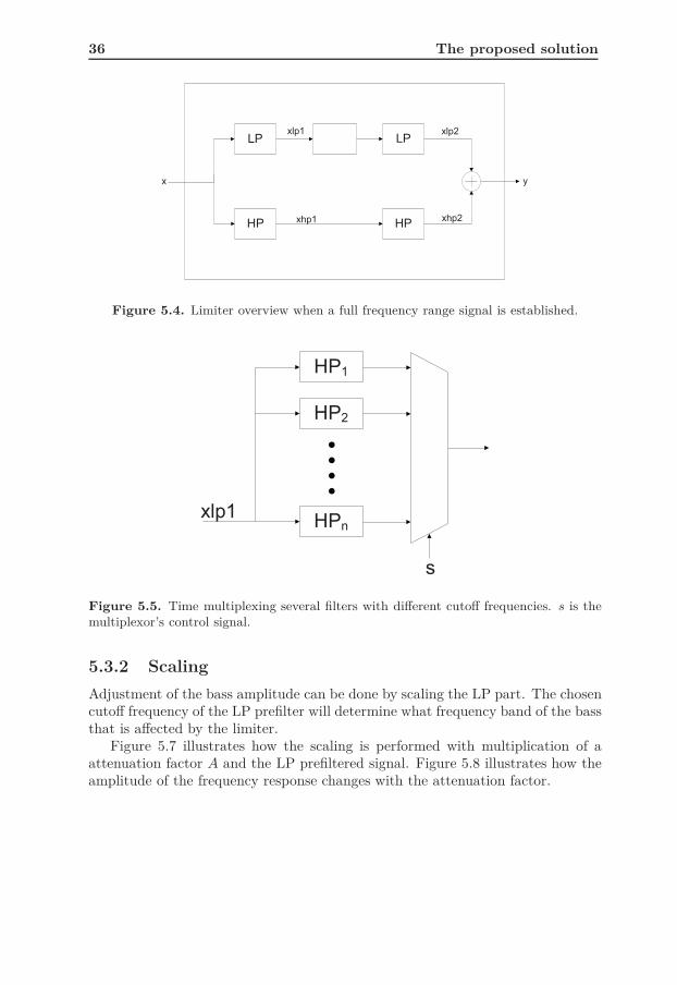
5.2.3 Preserving a full frequency range signal

In order to preserve a full range signal the HP part has to be added to the LPpart. The delay introduced by the LP filters has to be in same order as the delayintroduced by the HP filter, therefore two HP filters are added as seen in figure5.4.

5.3 Amplitude reduction of the bass channel

Disregarding how the decision is made whether to decrease bass or not, there area few straightforward ways of implementing a change of amplitude for the bassand they will be described in this section.

5.3 Amplitude reduction of the bass channel 35

0.16 0.165 0.17 0.175 0.18 0.185 0.19 0.195 0.2 0.205-1

-0.5

0

0.5

1

(a) Illustration of amplitude change on a sinusoid.

0.17 0.175 0.18 0.185 0.19 0.195 0.2 0.205 0.21-1

-0.5

0

0.5

1

(b) LP filtering of the same sinusoid where the amplitude has been changed.

Figure 5.2. Illustration of the effects of changing the amplitude and how LP filteringalleviates the clipping sound.

Figure 5.3. Limiter overview with a LP postfilter.

5.3.1 Time multiplexing

By using several HP filters with different cutoff frequencies between fc1 and fcn

where fc1 < fcn, the appropriate amount of attenuation can continuously be chosenby the control signal s. This is illustrated in figure 5.5 where the appropriate filteris selected and figure 5.6 illustrates how the frequency response changes when timemultiplexing HP filters.


Figure 5.4. Limiter overview when a full frequency range signal is established.

Figure 5.5. Time multiplexing several filters with different cutoff frequencies. s is themultiplexor’s control signal.

5.3.2 Scaling

Adjustment of the bass amplitude can be done by scaling the LP part. The chosencutoff frequency of the LP prefilter will determine what frequency band of the bassthat is affected by the limiter.

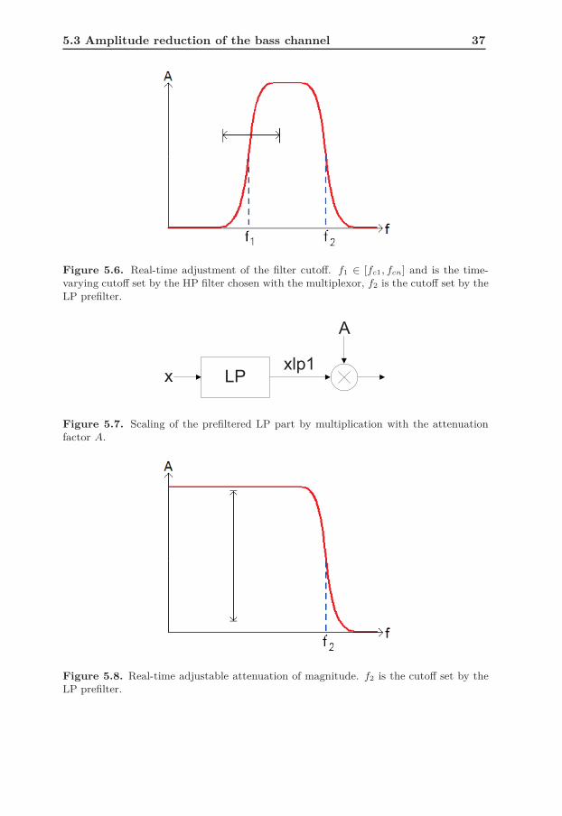
Figure 5.7 illustrates how the scaling is performed with multiplication of aattenuation factor A and the LP prefiltered signal. Figure 5.8 illustrates how theamplitude of the frequency response changes with the attenuation factor.

5.3 Amplitude reduction of the bass channel 37

Figure 5.6. Real-time adjustment of the filter cutoff. f1 ∈ [fc1, fcn] and is the time-varying cutoff set by the HP filter chosen with the multiplexor, f2 is the cutoff set by theLP prefilter.

Figure 5.7. Scaling of the prefiltered LP part by multiplication with the attenuationfactor A.

Figure 5.8. Real-time adjustable attenuation of magnitude. f2 is the cutoff set by theLP prefilter.


5.3.3 FFT and notch filter

Performing an FFT on the signal after the LP prefilter would reveal what frequencyis too strong. By applying a notch filter on top of this frequency the bass could beattenuated. The way of doing this would be according to the following procedure:

1. Create a buffer of the number of samples needed to perform an FFT.

2. Find the bass frequency with maximum magnitude.

3. Create a notch filter at this frequency.

4. Apply the notch filter.

5.3.4 Discussion and conclusions

All three methods listed above have their advantages and disadvantages which willbe briefly discussed here.

• Time multiplexing:

– Advantages:

1. Only the deepest bass is reduced to start with.

– Disadvantages:

1. A feedback system has to be implemented in order to know howmuch the bass is attenuated.

2. There is a delay between making the decision of attenuation andapplying the attenuation, especially if the bass to be reduced is ofhigh frequency and the selection of filters are switching from thelowest cutoff frequency to the highest.

3. The transparency of the sound within the bass band is altered whenattenuating certain frequencies.

• Scaling:

– Advantages:

1. Direct steering can be applied since the magnitude of the bass di-rectly shows how much it is over the allowed limit, hence how muchit has to be scaled down.

2. The delay is short between making the decision of attenuating andapplying the attenuation.

3. The transparency of the sound within the bass band is preservedsince only the amplitude of the bass is affected, not the frequencies.

– Disadvantages:

1. All frequencies in the bass is attenuated whether it is needed ornot.

5.4 Choice of filters 39

• FFT and notch:

– Advantages:

1. Only the frequencies causing distortion will be attenuated and therest of the bass is intact.

– Disadvantages:

1. A feedback system has to be implemented in order to know howmuch the bass is attenuated.

2. A longer delay is introduced when performing a FFT.

3. There might be several frequencies that are too strong and a deci-sion has to be made which ones to attenuate and how much.

4. The transparency of the sound within the bass band is altered whenattenuating certain frequencies.

After testing the different methods and evaluating how suitable they are forhardware implementation, the method of scaling the bass was chosen. The struc-ture of the limiter is now as in figure 5.9.

Figure 5.9. Overview of limiter with the chosen attenuation method.

5.4 Choice of filters

The choice of filters will be discussed in this section.

5.4.1 Crossover

The part of the signal that is subject to processing is first separated, thereaftersignal processing is performed. The signals are then mixed together again. Thesummed output should ideally be unchanged in both frequency, phase and relative


levels of amplitude compared to the original signal, i.e., a perfect crossover wouldbe ideal.

A commonly used method of implementing active audio crossovers is a designwith in-phase outputs and steep 24 dB/octave slopes. There are crossover offeringthe following characteristics:

1. Absolutely flat amplitude response throughout the passband with a steep 24dB/octave roll off rate after the crossover point.

2. The acoustic sum of the two driver responses is unity at crossover. (Ampli-tude response of each is -6 dB at crossover, i.e., there is no peaking in thesummed acoustic output.)

3. Zero phase difference between drivers at crossover.

4. The low pass and high pass outputs are always in phase.

The two drivers mentioned should here be thought of as the channels that areadded together in the last step of the limiter, adding up the signal y seen in figure5.9.

The crossover is however of non-linear phase. Research on the audible impactof slowly changing non-linear phase response shows that the audible results are sominimal as to be nonexistent; especially in comparison with all the other systemnon-linearities. With real world music sources, it is not audible at all [3].

With the facts above stated the choice of a crossover like this is reasonable.Each of the LP and HP filters in the limiter (see figure 5.9) are following the abovestated characteristics and together creating a crossover with flat amplitude.

The filters are realized with biquads, each requiring five coefficients. NS is usedin the biquad structure according to figure 2.2.

There are several reasons for not choosing FIR filter before IIR. First of all,IIR is, according to the discussion above, good enough for this purpose. Secondly,a FIR filter gives a longer delay, which is not desirable if preventable. A majorreason for keeping the delay to a minimum is synchronization between video motionand sound if the system is used as TV loudspeakers. A last reason for using IIRfilters and biquads is that the hardware structure still has to be implemented inActiwave’s FPGA system for reasons not concerning this thesis. Hence, it is agood choice to utilize a preexisting structure due to hardware limitations.

5.5 The decision making block

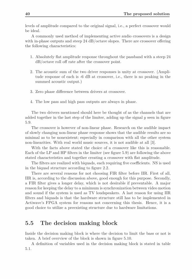
Inside the decision making block is where the decision to limit the bass or not istaken. A brief overview of the block is shown in figure 5.10.

A definition of variables used in the decision making block is stated in table5.1.

5.5 The decision making block 41

Figure 5.10. Overview of the decision making block.

Variable Definitionw A window of sampleslw Length of windowA(w) Attenuation in wmax(w) Maximum value in wthreshold Threshold set for limiting samplesm Number of old maximum values stored

Table 5.1. Definition of variables used the decision making block.

5.5.1 The maximum block

The maximum block is continuously identifying and storing the maximum absolutevalue of incoming samples. The internally stored maximum sample value, max,is reset on every lw samples and a new maximum value is then available on theoutput port. Every window w has its own max ∈ [0, 1[. Equation 5.1 defines howmax is calculated.

max(w) = maximum|x(n)|, |x(n + 1)| . . . , |x(n + (lw − 1))| (5.1)

The choice of letting the limiter react on peak values are motivated by the fastattack time required. Other options are to react on an average value or a RMSvalue in a window w. This would however give a slower response and peaks couldeasily slip through and cause distortion without being detected by the limiter.

5.5.2 Direct steering

A direct steering is applied when calculating the attenuation factor A. The attackand release of the A is described in this section.


Attack

Any sample values over the threshold is counteracted by a decrease of the atten-uation factor A, i.e. an attack, according to equation 5.2.

A =

1, if max ≤ thresholdthreshold

max, if max > threshold

(5.2)

The factor An, in a given sample window wn, is multiplied with the samplesvalues in the same sample window wn. This requires a delay of the signal of thelength lw to guarantee that no sample values leaving the limiter is larger than thethreshold. The delay is however left out, and An is applied to window wn+1 (onewindow after wn). This could result in sample values over the threshold, but itwould only be a problem if the window w is wide. The window length lw shouldbe chosen short enough to achieve a fast response time. The attenuation delay is,depending on tuning of the limiter (the value of lw), in the order of what is givenin equation 5.3.

Attenuation delay ≤lwfs

=N

44100 Hz(5.3)

Release

There are however restrictions in the direct steering when in comes to the release.A decrease of A (an attack) is always allowed since the system has to be able tolimit any sample values that are too large. But an increase of A (a release) cannotalways be allowed since it might cause unnecessary switching of A.

A few of the latest max-values will be taken into consideration if a release isimplied by maxn in wn. The following equation is valid for switching A in a release.

An = thresholdmaximummaxn−m,...,maxn , where m > 1

Figure 5.11 shows a sinusoid of constant amplitude and illustrates how the last5 maximum values (m = 5) are taken into consideration.

Equation 5.4 shows the relation between, lw, m and the lowest frequency, fl,to be played by the system.

lw = dfs

fl

/2(m + 1)e (5.4)

The question of how many old maximums that should be taken into consider-ation is a matter of tuning.

5.6 Optional functionality

It is illustrated in section 5.2.2 and figure 5.2(a) how a change of amplitude causesdiscontinuities in the waveform. One way of mitigating this is to change the

5.7 The volume control 43

Figure 5.11. A constant amplitude sinusoid with a number of windows w and belongingmax-values. m = 5 in this illustration and the A factor is held between the peaks sinceone of the latest five (m) maximums are one (1) when a release is implied in between thepeaks of the sinusoid.

amplitude in the zero crossings of the signal. There is however no guarantee thata zero crossing is available in a specific short instance of time after the change ofA is implied. Thus, a change of A might be forced before a window w of time haspast.

5.7 The volume control

First of all, the position of the limiter should be before the volume control. Ageneric sample is in the interval [−1, 1[ and the volume is adjusted by multiplyingthe sample value with a factor smaller than one (1). In order to not reduce theresolution of the sample values, the multiplication is the last operation one wantto perform before leaving the digital domain.

The limiter will be placed before the volume multiplication in the audio chain.Therefore, the volume has to be taken into consideration inside the limiter. Thisis done by simply multiplying the max-value with the volume factor. However,this feature has been left out in Simulink models since the limiter isn’t working inreal-time and the simulations work with a fix volume level.


5.8 The complete limiter

An overview of the complete limiter derived in this chapter is seen in figure 5.12.

Figure 5.12. An overview of the complete limiter.

5.9 Limiter simulations

A few simulation cases will in this section illustrate the functionality of the limiterdeveloped in Simulink. As earlier mentioned, the Simulink model has no volumecontrol, i.e., the simulations are performed with constant volume. The chosenthreshold in these simulations is 0.42.

5.9 Limiter simulations 45

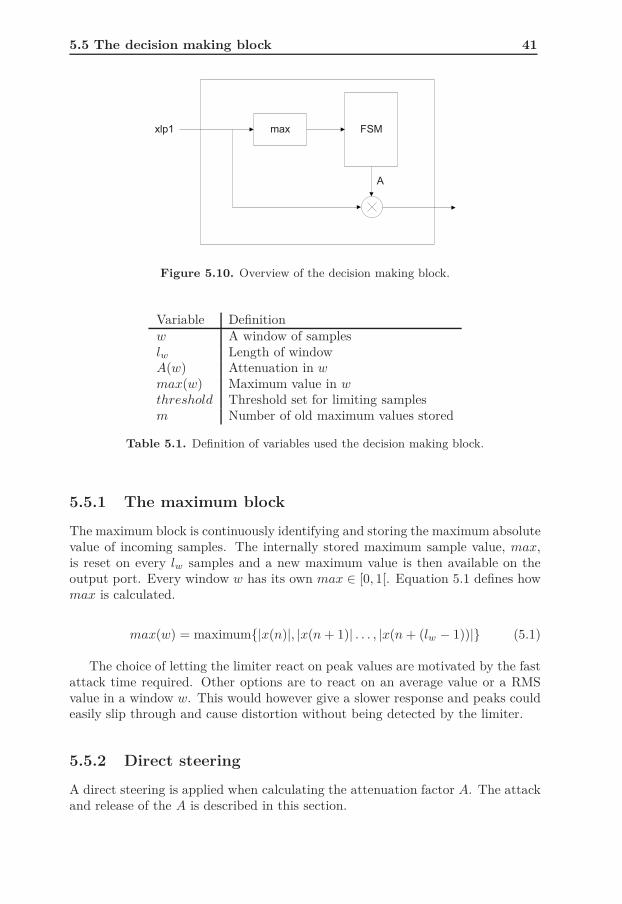
5.9.1 Limitation of a sinusoid with constant amplitude

The limitation of a sinusoid with constant amplitude is seen in figure 5.13.

0.05 0.055 0.06 0.065 0.07 0.075 0.08 0.085 0.09 0.095 0.1-1

-0.5

0

0.5

1

t

x

(a) The input signal x = sin(2π50).

0.05 0.055 0.06 0.065 0.07 0.075 0.08 0.085 0.09 0.095 0.10

0.5

1

t

A

(b) The attenuation factor A.

0.05 0.055 0.06 0.065 0.07 0.075 0.08 0.085 0.09 0.095 0.1-1

-0.5

0

0.5

1

t

y

(c) The limited output signal y ≈ 0.42sin(2π50).

Figure 5.13. Simulations of the limiter when the input is a sinusoid with constantamplitude.

In figure 5.13(b), notice how A is held constant and that the amplitude of thesinusoid is approximately at the threshold.


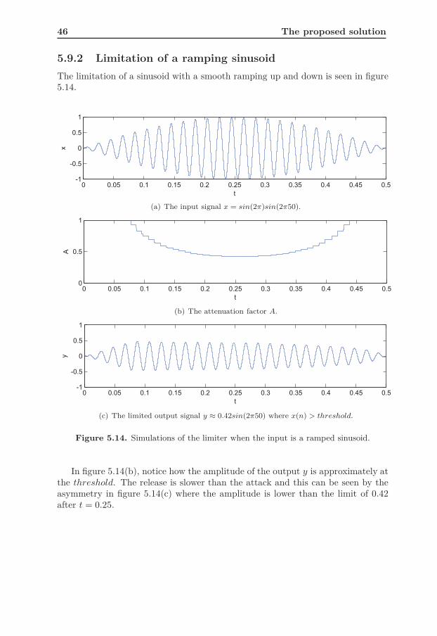
5.9.2 Limitation of a ramping sinusoid

The limitation of a sinusoid with a smooth ramping up and down is seen in figure5.14.

0 0.05 0.1 0.15 0.2 0.25 0.3 0.35 0.4 0.45 0.5-1

-0.5

0

0.5

1

t

x

(a) The input signal x = sin(2π)sin(2π50).

0 0.05 0.1 0.15 0.2 0.25 0.3 0.35 0.4 0.45 0.50

0.5

1

t

A

(b) The attenuation factor A.

0 0.05 0.1 0.15 0.2 0.25 0.3 0.35 0.4 0.45 0.5-1

-0.5

0

0.5

1

t

y

(c) The limited output signal y ≈ 0.42sin(2π50) where x(n) > threshold.

Figure 5.14. Simulations of the limiter when the input is a ramped sinusoid.

In figure 5.14(b), notice how the amplitude of the output y is approximately atthe threshold. The release is slower than the attack and this can be seen by theasymmetry in figure 5.14(c) where the amplitude is lower than the limit of 0.42after t = 0.25.

5.10 Conclusion 47

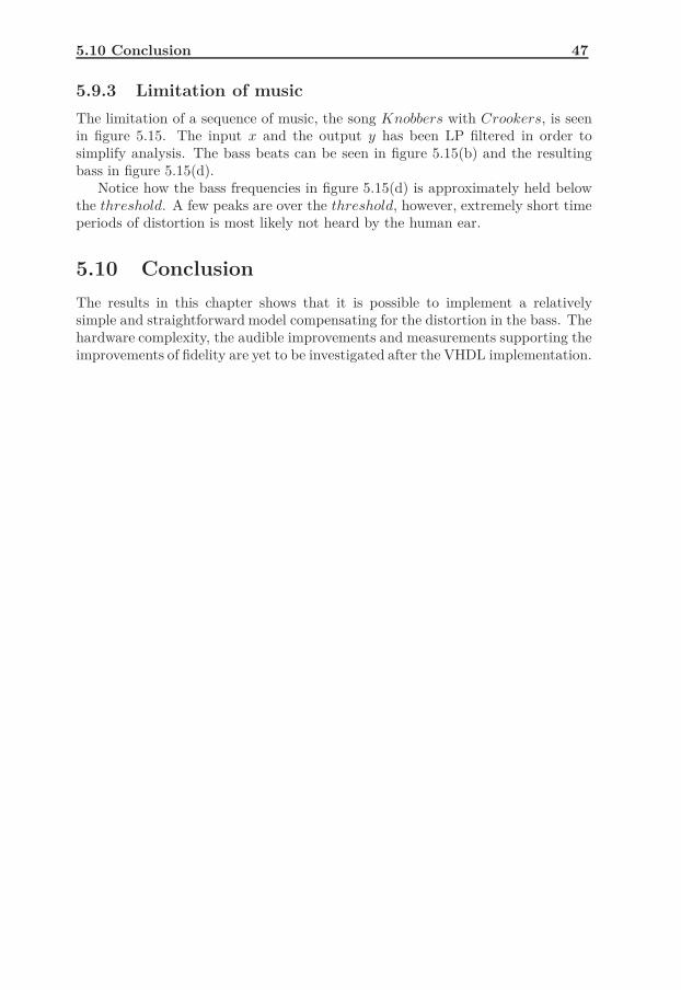
5.9.3 Limitation of music

The limitation of a sequence of music, the song Knobbers with Crookers, is seenin figure 5.15. The input x and the output y has been LP filtered in order tosimplify analysis. The bass beats can be seen in figure 5.15(b) and the resultingbass in figure 5.15(d).

Notice how the bass frequencies in figure 5.15(d) is approximately held belowthe threshold. A few peaks are over the threshold, however, extremely short timeperiods of distortion is most likely not heard by the human ear.

5.10 Conclusion

The results in this chapter shows that it is possible to implement a relativelysimple and straightforward model compensating for the distortion in the bass. Thehardware complexity, the audible improvements and measurements supporting theimprovements of fidelity are yet to be investigated after the VHDL implementation.


0.9 1 1.1 1.2 1.3 1.4 1.5 1.6-1

-0.5

0

0.5

1

t

x

(a) The input signal.

0.9 1 1.1 1.2 1.3 1.4 1.5 1.6-1

-0.5

0

0.5

1

t

x

(b) The input signal LP filtered.

0.9 1 1.1 1.2 1.3 1.4 1.5 1.60

0.5

1

t

A

(c) The attenuation factor A.

0.9 1 1.1 1.2 1.3 1.4 1.5 1.6-1

-0.5

0

0.5

1

t

y

(d) The limited output signal LP filtered.

0.9 1 1.1 1.2 1.3 1.4 1.5 1.6-1

-0.5

0

0.5

1

t

y

(e) The limited output signal.

Figure 5.15. Simulations of the limiter when the input is a music sequence.

Chapter 6

VHDL implementation

This chapter will briefly describe the implementation of the limiter in VHDL. Themodule was interconnected with already existing VHDL modules and some prop-erties such as word lengths are inherited from the existing system. The completeaudio chain is basically given even if changes had to be done to instantiate thelimiter. An overview of the complete system is seen in figure 6.1.

Figure 6.1. An overview of the existing VHDL environment where the limiter is in-stantiated. The dashed blocks are generally in the system, but are not used in thisthesis.

6.1 FPGA

The FPGA used during development was a Xilinx Spartan 3 XC3S250E, but thelimiter will later be implemented on a larger Spartan 6. Changes to the VHDL codemay have to be performed in order to optimize for the new hardware environment.

6.2 Clock domains

The system operates on a 50 MHz clock and the sample clock. Typically thesample rate is 44100 Hz. In that case, there is about 1133 system clock periods onevery sample clock period. This gives time for a lot of processing until the nextsample clock arrives. Thus, there is no particular time-restraint to adapt to in thissystem when processing data.

A third clock is created by dividing the sample clock and thus creating thewindow w used for continuously finding maximum values in the input sequence.

49

50 VHDL implementation

6.3 Implementation and optimization

This section will describe the most important parts of the implementation.

6.3.1 Biquads

The biquad filter structure was given by Actiwave but needed modifications. Thefilter was modified to be able to sequentially execute several inputs with differentsets of filter coefficients while using the same hardware for each filter execution.It is possible to execute 62 filters during one sample clock period with the samehardware.

The filter coefficients and the internal data in the biquad’s memories are storedin a block ram.

It is also possible to execute a filter an arbitrary number of times (in cascade)in the biqaud structure. Hence, the HP filters seen in figure 5.12 only needs oneset of coefficients since the biquad will run it twice instead of instantiating twoseparate filters.

6.3.2 Decision making block

The first model implemented had, like the software implementation, a large res-olution of the max-values. This resolution is far more than needed when settingthe attenuation factor A.

The first implementation used an if statement in order to create steps of atten-uation for the maximum values above the threshold. Performing a series of audibletests where the volume was changed in small steps, a limit of a minimum audiblevolume step was found. An attenuation step much smaller than the minimumaudible volume change is unnecessary and a waste of hardware.

In order to reduce hardware utilization, the max-values was scaled down, andhence the amount of attenuation factors was reduced. With these changes themax-value can be used directly as an address to a block ram where the coefficients(attenuation factors) are stored.

6.3.3 Miscellaneous

The other parts of the hardware are quite straightforward and no deeper explana-tion is given than the one below.

• ScalingThe scaling of the signal is constructed by an IP core multiplier and an FSMrunning the data path.

• Crossover additionThe addition of the two frequency bands, together creating a flat amplituderesponse, is instantiated by an IP core adder.

Further optimization has been to remove unnecessary processes, keeping theword length of signals as small as possible and optimize code in general.

6.4 Volume control 51

6.4 Volume control

There is no volume control in the VHDL system given by Actiwave. If one wasgiven, it would, according to earlier discussion in section 5.7 be positioned as lateas possible in the audio data chain.

The future volume control will simply be a multiplication of the current volumefactor and the incoming max-value that is of full swing. If this is not performed,the limiter will be activated even though the volume might be quite low.

Chapter 7

THD measurements

The results of the limiter has throughout the work in this thesis mainly beenbased on the perceived experience of the sound. This chapter will present THDmeasurements proving the actual functionality of the limiter.

7.1 Introduction to THD measurements

The THD is often measured at a specific sound pressure level (SPL) in orderto be able to compare results achieved at different occasions and on differentloudspeakers. For example, a THD measurement done at 96 dB on 1 meter is equalto a measurement at 90 dB at 2 meters. 90 dB is however quite loud and nothingone listens to normally. In this case, the conditions of the THD measurementsonly needs to be the same when performed at different occasions in order to havefair comparisons.

A THD of 10 % is normally a threshold value for the amplifiers maximum out-put power. This measurement is however not of interest in this thesis. The THDmeasurement performed here is also including the distortion of the loudspeakerand not only the amplifier’s THD.

The question of how low the THD should be in order to be reasonably goodis not a matter of discussion here. It is only of interest to compare results whenthe limiter is on or off. The given test speaker, loudspeaker A, is of low qualityand a high THD will be met at low levels of volume for low frequencies. Higherfrequencies are however reproduced with higher fidelity with loudspeaker A.

7.2 THD measurement

A relevant test is to measure the THD for different volumes and different fre-quencies with and without the limiter. The limiter should, if working correctly,prevent clipping of the signal, and limit the output voltage to a specific level. Theunlimited signal can however be clipped and cause much distortion.

53

54 THD measurements

7.2.1 Data collection

Amplifier C and loudspeaker A was used in the test and the THD measurementwas performed with the freeware ARTA.

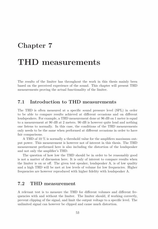
The results of the test can be seen in table 7.1. The volume in the table isreferred to the amplitude of the tone (the digital sample value in the interval of[−1, 1[). THD was measured for four frequencies (30, 50, 70, 90 Hz).

THD [%]Without limiter With limiter

V olume \ f 30 50 70 90 30 50 70 900.1 9 4 8 1 10 5 8 10.2 10 9 15 2 10 9 14 20.3 15 15 21 3 15 14 21 30.4 24 25 33 5 23 24 32 40.5 40 36 45 6 27 28 37 50.6 ≥ 100 ≥ 100 61 12 27 28 38 60.7 . . 94 23 27 29 38 60.8 . . ≥ 100 32 27 29 38 60.9 . . . 40 27 29 38 61.0 . . . 45 27 29 38 6

Table 7.1. The table shows the THD for the frequencies 30, 50, 70 and 90 Hz whenplaying at different volumes with and without the limiter.

The results in table 7.1 proves that the limiter limits the digital sample valuesand hence the maximum output voltage and by this reduces the distortion of theoutput signal. There is no limit of the voltage without the limiter, except themaximum voltage, hence the distortion is growing until it is no longer possible toincrease the volume.

A THD larger than 100 % is possible depending of what definition is used. Thefreeware ARTA uses equation 2.5.

There are other sources of THD in the audio system except the one belongingto the clipping. These non-linearities are however equal, independent of whenplaying with the limiter or not. Hence, it is the difference between the measuredlevels of THD that is of interest when comparing the result, not the source itself.

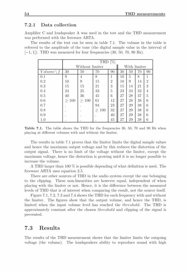
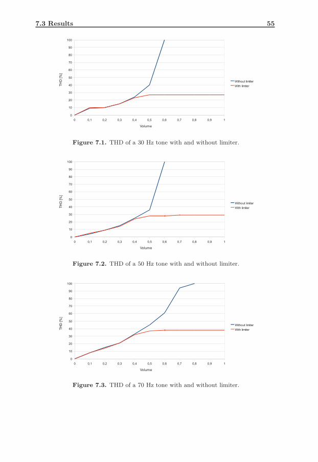
Figure 7.1, 7.2, 7.3 and 7.4 shows the THD for each frequency with and withoutthe limiter. The figures show that the output volume, and hence the THD, islimited when the input volume level has reached the threshold. The THD isapproximately constant after the chosen threshold and clipping of the signal isprevented.

7.3 Results

The results of the THD measurement shows that the limiter limits the outgoingvoltage (the volume). The loudspeakers ability to reproduce sound with high

7.3 Results 55

0 0,1 0,2 0,3 0,4 0,5 0,6 0,7 0,8 0,9 1

0

10

20

30

40

50

60

70

80

90

100

Without limiter

With limiter

Volume

TH

D [%

]

Figure 7.1. THD of a 30 Hz tone with and without limiter.

0 0,1 0,2 0,3 0,4 0,5 0,6 0,7 0,8 0,9 1

0

10

20

30

40

50

60

70

80

90

100

Without limiter

With limiter

Volume

TH

D [%

]


0 0,1 0,2 0,3 0,4 0,5 0,6 0,7 0,8 0,9 1

0

10

20

30

40

50

60

70

80

90

100

Without limiter

With limiter

Volume

TH

D [%

]


56 THD measurements

0 0,1 0,2 0,3 0,4 0,5 0,6 0,7 0,8 0,9 1

0

10

20

30

40

50

60

70

80

90

100

Without limiter

With limiter

Volume

TH

D [%

]


fidelity is likely to vary over the frequency range with the systems properties andthis can be seen since the THD is largest for 70 Hz and a volume of 0.5. Hence,the lowest frequencies does not necessarily give the largest THD. However, theresults show that the barrier of 100 % THD is met at higher volume for higherfrequencies, hence the audio system is better at reproducing high frequencies thanlow at a high volume.

Chapter 8

Conclusions and discussion

The results in the previous chapters shows that it is possible to implement a lowcost hardware module that in real-time detects when the bass will cause distor-tion and compensates for it. The implemented model gave satisfying results andimproved the fidelity of the sound while playing at a very high volume. At thesame time it lead to a flexible and efficient hardware solution.

The developed model, the model’s properties, the VHDL implementation, con-clusions and future work will be discussed in this chapter.

8.1 Audible improvement

According to the authors, the perceived experience of the sound is dramaticallyimproved. However, a few things are worth mentioning about the differences inthe bass while using the limiter or not.

By comparing a limited system against the same system without the limiterapplied there is a considerable difference. Without the limiter it is possible toturn up the volume more and more. The audible distortion in the bass beats willincrease and make a crackling sound. The music is perceived as loud, but thelistener will realize that the system is working outside its range of fidelity.

Playing music with the limiter will prevent the crackling distortion from aris-ing. The loudspeaker sounds more controlled and unpleasant high frequencies areremoved. The experience may however be that even if the volume is turned upthe bass isn’t increasing. The listener might be disappointed by the fact that theoutput is limited. However, the purpose of the limiter is to compensate systemsor amplifiers with obvious limitations in output power.

Extremely short bursts of distortion is most likely no problem for the listenersince the human ear can’t detect them. The question of how short these burstscan be and how sensitive the ear is, is not a subject for discussion in this thesis.However, the user of the limiter should consider how limited the system shouldbe. Maybe just a little distortion can be allowed in order to give the listener thefeeling of really pushing the system to its edge.

57

58 Conclusions and discussion

What about the audible differences? Has it made the experience of the soundbetter or worse? In a more general question, how does the audio system soundwith the limiter applied? These questions are subjective and the answers dependon the listener’s perception of sound. The matter of tuning the limiter is up to thedesigner of the audio system. It might often be a trial and error situation whenplaying different music with different limiter settings.

8.2 Regarding the model

Several models have been developed during the work with this thesis and a fewmodels were implemented in VHDL. All the models’ combined properties and ad-vantages regarding both complexity and functionality lead to the proposed solutionthat is subject of discussion in this section.

8.2.1 Functionality of the model

The following main properties has been fulfilled with the proposed model devel-oped.

• Establishing a full range signal after the limitation in order to be able to usethe limiter in any kind of audio system where the loudspeakers have differentfrequency ranges.

• Attenuate the bass when necessary without causing any audible distortionfrom the compensation itself and hence preserving the perceived fidelity ofthe sound.

• Preserve a flat frequency response and avoid phase delay that alters theperceived sound.

• Provide a flexible system open for further improvements and developments.

8.2.2 Future work and discussion

• An advantage with the proposed model, which scales the amplitude in afrequency band, compared to the model where the bass is cut from thelowest frequencies and up (see figure 5.8), is that it can be applied on anydesirable frequency band.

This can be performed by changing the filters and the detector (RMS, aver-age, peak). This would not be possible with the method of cutting the bassaccording to figure 5.8.

• While investigating the HP part of the signal it was found that the prob-lems of distortion that occur in the HP part cannot always be related toits amplitude alone. For example, there might occur high frequency signalinformation looking more like square waves while bass signals tend to lookmore like nicely shaped sinusoids. The problem with the square waves are

8.2 Regarding the model 59

not that they simply just peak over the allowed threshold and cause dis-tortion, but rather that the area under them is very large. This yields aninstantaneous power consumption that might be over the amplifier stage’sability. The closer the amplifier stage is pushed to its limit, the more dis-tortion arises. Eventually a shut down of the amplifier stage will occur if itis pushed too hard. It is however relatively easy to alleviate this problemusing a modified version of the developed limiter.

• Looking at figure 7.1 and 7.4 shows that the distortion is lower at the samevolume for high frequencies than for low. Setting one threshold for a widefrequency band is an approximation. Lower frequencies tend to need lowerthreshold and the distortion does most likely not only depend on the outputvoltage being to close to the maximum voltage in the amplifier, but it alsodepends on the power consumption instantaneously drawn from the powerstage. Using only the amplitude as a decision maker works for low frequenciesbut higher frequencies might need a power consumption detector.

• The zero crossing block tries to apply the attenuation factor where it willcause the least harm, i.e., when there is a zero crossing in the signal. If azero crossing isn’t found, the attenuation factor will be forced to be appliedafter a specific time. An audible difference while using the zero crossingfunctionality has not been detected.

• A problem encountered with the biquad filters are their sensitivity. Filtersof low cutoff frequency are susceptible to quantization error, mainly fromthe feedback coefficients b1 and b2. Lack of resolution in the coefficientsmakes a precise positioning of the poles difficult. NS, which is implementedin the biquad structure used, is a technique alleviating this. The NS isn’tgood enough if very low cutoff frequencies are chosen and then the filtercoefficient word length has to be increased.

• An overall optimization should be performed when the limiter is implementedin the final system.

• There is no soft knee start of applied attenuation, i.e., a slowly increasingattenuation, in the developed limiter. Using a model where the bass is in-creasingly attenuated with a start at low amplitudes will minimize theseproblems. Although, this would remove bass when it is not necessary. Thisis not desirable and therefore this type of early attenuation was not imple-mented.

Another possible problem with the proposed model is the disregarded delaybetween the window w where A is calculated and the appliance of A on thesignal. This could cause signal peaks to pass through and cause audibledistortion. It is however easy to correct if it is found to be a source ofdistortion.

60 Conclusions and discussion

8.3 Supplementary conclusion

Although we are satisfied with the result of our implementation there are issuesto be considered. The system will effectively compensate for distortion caused bytoo much bass, but it will not guarantee that higher frequencies won’t give riseto the same sort of problem. With the proposed solution’s functionality higherfrequencies will be unmodified.

The designer have to consider that it is not the amplitude in separate fre-quency bands that cause distortion but the total signal level reaching the am-plifier. Therefore, a volume limitation is needed unless a limiter is used on thecomplete frequency band. A system does always have a limit of how loud it canplay, either because of distortion that occurs or simply because it shuts down attoo high power consumption. A well tuned limiter in the bass band together witha volume limitation is most likely a satisfactory solution.

There is an uncertainty in how this model will work on different amplifierswith different loudspeakers since it has only been tested on one system. And eventhough some work is still left before a completely compensated system is achieved,we, the authors, believe that the developed limiter with its current functionalityis fully operational and solves the given problem satisfactory.

Bibliography

[1] Bengt Molin. Analog Elektronik. Studentlitteratur, 2001.

[2] David E. Reese, Lynne S. Gross, Brian Gross. Audio Production Worktext,6th Edition. Focal Press, 2009.

[3] Dennis Bohn. Linkwitz-Riley Crossover: A Primer. Rane Corporation,http://www.rane.com/note160.html, February 2010.

[4] Digiteo. The Scilab Consortium. http://www.scilab.org/products/scilab,February 2010.

[5] Earlevel Engineering. Biquad forms. www.earlevel.com, February 2010.

[6] F. Alton Everest. The Master Handbook of Acoustics, 4th Edition. TheMcGraw-Hill Companies, 2001.

[7] Håkan Johansson. Discrete-Time Systems. Elektronic Systems, Departmentof Electrical Engineering, Linköpings University, 2009.

[8] Ivo Mateljan. Audio Measurement and Analysis Software.http://www.fesb.hr/ mateljan/arta/index.htm, January 2010.

[9] John Eargle. Loudspeaker handbook. Kluwer Academic Pulblishers, 2003.

[10] John F. Allen. Total distortion in modern theatre woofer systems. Boxofficemagazine, 1992.

[11] Lars Wanhammar. Analog filters using Matlab. Prepublication Version, 2008.

[12] Lars Wanhammar and Håkan Johansson. Digital Filters. Department ofElectrical Engineering, Linköping University, 2007.

[13] Lloyd Butler. Intermodulation Performance and Measurement of Intermodu-lation Components. Amateur Radio, August 1997.

[14] M-Audio. M-Audio Firewire 410 Manual. http://www.m-audio.com/, Jan-uary 2010.

[15] Paradigm. Product Sheet Cinema 110 L/R. http://www.paradigm.com/,January 2010.

61

62 Bibliography

[16] Paul White. Advanced Compression Techniques Part 1. Sound On Sound,http://www.sospubs.co.uk/sos/dec00/articles/adcompression.htm, 2000.

[17] Ruurd de Vries, Arthur P. Berkhoff, Cornelis H. Slump, Otto E. Herrman.Digital compensation of nonlinear distortion in loudspeakers. Departmentof Electrical Engineering, University of Twente, Enschede, the Netherlands,1999.

[18] Scott Lehman. Compression Limiting. Harmony Central,http://www.harmony-central.com/Effects/Articles/Compression/, February2010.

[19] Soundstage. How we test loudspeakers. http://www.soundstagenetwork.com/measurements/test_loudspeakers.htm, January 2010.

[20] Sune Söderkvist. Kretsteori och Elektronik. Tryckeriet Erik Larsson AB,1999.

[21] Sune Söderkvist. Från insignal till utsignal. Tryckeriet Erik Larsson AB,2007.

[22] Texas Instrument. 20 W Stereo Digital Amplifier Power Stage TAS5602.http://www.ti.com/, January 2010.

[23] The Mathworks. Simulink - Simulation and model-based design.http://www.mathworks.com/products/simulink/, February 2010.

[24] Walt G. Jung. Op Amp applications handbook. Analog Devices, 2004.

[25] Xilinx. ISE Webpack Design Software. http://www.xilinx.com/tools/webpack.htm, February 2010.

[26] Yamaha. Product Sheet Yamaha AV Receiver RX-V630RDS.https://www.yamaha.com, January 2010.

Upphovsrätt

Detta dokument hålls tillgängligt på Internet — eller dess framtida ersättare —under 25 år från publiceringsdatum under förutsättning att inga extraordinäraomständigheter uppstår.

Tillgång till dokumentet innebär tillstånd för var och en att läsa, ladda ner,skriva ut enstaka kopior för enskilt bruk och att använda det oförändrat för icke-kommersiell forskning och för undervisning. Överföring av upphovsrätten vid ensenare tidpunkt kan inte upphäva detta tillstånd. All annan användning av doku-mentet kräver upphovsmannens medgivande. För att garantera äktheten, säkerhe-ten och tillgängligheten finns det lösningar av teknisk och administrativ art.

Upphovsmannens ideella rätt innefattar rätt att bli nämnd som upphovsmani den omfattning som god sed kräver vid användning av dokumentet på ovan be-skrivna sätt samt skydd mot att dokumentet ändras eller presenteras i sådan formeller i sådant sammanhang som är kränkande för upphovsmannens litterära ellerkonstnärliga anseende eller egenart.

För ytterligare information om Linköping University Electronic Press se förla-gets hemsida http://www.ep.liu.se/

Copyright

The publishers will keep this document online on the Internet — or its possi-ble replacement — for a period of 25 years from the date of publication barringexceptional circumstances.

The online availability of the document implies a permanent permission foranyone to read, to download, to print out single copies for his/her own use andto use it unchanged for any non-commercial research and educational purpose.Subsequent transfers of copyright cannot revoke this permission. All other uses ofthe document are conditional on the consent of the copyright owner. The publisherhas taken technical and administrative measures to assure authenticity, securityand accessibility.

According to intellectual property law the author has the right to be mentionedwhen his/her work is accessed as described above and to be protected againstinfringement.

For additional information about the Linköping University Electronic Pressand its procedures for publication and for assurance of document integrity, pleaserefer to its www home page: http://www.ep.liu.se/

c© Fredrik Bengtsson and Rikard Berglund

Documents

Digital compensation of distortion in audio systems318711/FULLTEXT01.pdf · Digital compensation of distortion in audio ... 5.9.1 Limitation of a sinusoid ... Investigate how a too