Differential Point RenderingAravind Kalaiah Amitabh Varshney

University of Maryland1

Abstract. We present a novel point rendering primitive, calledDifferentialPoint (DP), that captures the local differential geometry in the vicinity of a sam-pled point. This is a more general point representation that, for the cost of afew additional bytes, packs much more information per point than the traditionalpoint-based models. This information is used to efficiently render the surface asa collection of local neighborhoods. The advantages to this representation aremanyfold: (1) it delivers a significant reduction in the number of point primi-tives that represent a surface (2) it achieves robust hardware accelerated per-pixelshading – even with no connectivity information (3) it offers a novel point-basedsimplification technique that has a convenient and intuitive interface for the userto efficiently resolve the speed versus quality tradeoff. The number of primitivesbeing equal, DPs produce a much better quality of rendering than a pure splat-based approach. Visual appearances being similar, DPs are about two times fasterand require about75% less disk space in comparison to splatting primitives.

1 Introduction

Point-based rendering schemes [5, 12, 13, 17, 19, 21] have evolved as a viable alter-native to triangle-based representations. They offer many benefits over triangle-basedmodels: (1) efficiency in modeling and rendering complex environments, (2) hierar-chical organization to efficiently control frame-rates and visual quality, and (3) zero-connectivity for efficient streaming for remote rendering [20].

Current point primitives store only limited information about their immediate local-ity, such as normal, bounding ball [19], and tangent plane disk [17]. These primitivesare then rasterized with flat shading and hence such representations require very highsampling to obtain a good rendering quality. In other words, the rendering algorithmdictates the sampling frequency of the modeling stage. This is clearly undesirable as itmay prescribe very high sampling even in areas of low spatial frequency, causing twosignificant drawbacks: (1) slower rendering speed due to higher rendering computationand related CPU-memory bus activity, and (2) large disk and memory utilization.

In this work we propose an approach of storing local differential geometric infor-mation with every point. This information gives a good approximation of the surfacedistribution in the vicinity of each sampled point which is then used for rendering thepoint and its approximated vicinity. The extent of the approximated vicinity is deter-mined by the curvature characteristics of the surface: points in a flat or a low curvatureregion approximate larger vicinities. Our approach has many benefits to offer:

1Graphics and Visual Informatics Laboratory, Department of Computer Science and UMIACS, Universityof Maryland, College Park, MD - 20742, USA,fark,varshneyg@cs.umd.edu

1. Rendering: Our approach achieves high rendering quality with per-pixel shading.We reduce the number of rendering primitives and push more computation into eachprimitive. This reduces the CPU-memory bus bandwidth and the overall amount ofcomputation resulting in a significant speed-up. As the processor-memory speedgap increases we expect this method to get even more attractive.

2. Storage: The reduction in the number of primitives more than compensates for theextra bytes of information stored with each point primitive. This leads to an overallreduction in the storage requirements. This reduction also benefits faster streamingof information over the network.

3. Generality: The information stored with our point primitives is sufficient to derive(directly or indirectly) the requisite information for prior point primitives. Our workis primarily a focus on the efficiency of per-point rendering computation. It canpotentially be used in conjunction with larger point-based organization structures -hierarchical [1, 17, 19] or otherwise [13, 21].In the following sections, we first mention some related works and then outline the

terminology from the differential geometry literature that will be used to describe ourapproach. This is followed by a discussion of differential points. We then describeour rendering algorithm and compare it with some splatting schemes. We conclude thepaper with a discussion of this approach and its potential extensions.

2 Related Work

Classical differential geometry gives us a mathematical model for understanding thesurface variation at a point. Surface curvatures can be accurately computed for paramet-ric surfaces and can also be estimated from discrete sampled representations.Taubin [22]estimates curvature at a mesh vertex by using the eigenvalues of an approximationmatrix constructed using the incident edges. Desbrun et al. [3] define discrete oper-ators (normal, curvature, etc.) of differential geometry using Voronoi cells and finite-element/finite-volume methods.

Various hierarchical organization schemes have been used that develop lower fre-quency versions of the original set of point samples [1, 17, 19]. We use a simplificationprocess that prunes an initial set of points to greatly reduce the redundancy in surfacerepresentation. Turk [23] uses a point placement approach with the point density beingcontrolled by the local curvature properties of the surface. Witkin and Heckbert [24]use physical properties of a particle system to place points on an implicit surface.

Image-assisted organization of points [5, 13, 21] are efficient at three-dimensionaltransformations as they use the implicitness of relationship among pixels to achieve fastincremental computations. They are also efficient at representing complex real-worldenvironments. The multiresolution organizations [1, 17, 19] use their hierarchical struc-ture to achieve block culling, to control depth traversals to respect the image-qualityor frame-rate constraints, and for efficient streaming of large datasets across the net-work [20].

Darsa et al. [2], Mark et al. [14] and Pulli et al. [18] use a triangle mesh overlaidon the image sampling plane for rendering. It can be followed by a screen space com-positing process. However, such systems can be expensive in computation and storageif high resolutions are desired. Levoy and Whitted [12] introduced points as a renderingprimitive. It has been used by Shade et al. [21] and Grossman and Dally [5] for syn-thetic environments. However, raw point primitives suffer from aliasing problems andholes. Lischinski and Rappoport [13] raytrace a point dataset. Oliveira et al. [15] use

image space transformations to render point samples. Rusinkiewicz and Levoy [19] usesplatting of polygonal primitives for rendering. Pfister et al. [17] follow up the splattingwith a screen-space filtering process to handle holes and aliasing problems. Zwickeret al. [25] derive a screen-space formulation of the EWA filter to render high detailtextured point samples with a support for transparency.

3 Differential Geometry for Surface Representation

Fig. 1. Neighborhood of a Differential Point

Classical differential geometry is a studyof the local properties of curves and sur-faces [4]. It uses differential calculus offirst and higher orders for this study. In thiswork we use the regular surface model whichcaptures surface attributes such as continu-ity, smoothness, and degree of local surfacevariation. A regular surfaceis a differen-tiable surface which is non self-intersectingand which has a unique tangent plane at eachpoint on the surface. Every pointp on theregular surface has the following properties:the normalNp, the direction of maximumcurvatureup, thedirection of minimum cur-vature vp, the maximum normal curvature

�up , and theminimum normal curvature�vp . They have the following relation amongstthem: (1)j�up j � j�vp j, (2) hup; vpi = 0, and (3)up � vp = Np whereh�; �i denotes thedot product and� is the cross product operator. The differential of the normal atp isdenoted bydNp. Given any tangentt (= tuup + tvvp), dNp(t) is the first-order normalvariation aroundp and is given by [4]:

dNp(t) = �(�uptuup + �vptvvp) (1)

Similarly the normal curvature alongt, �p(t), is given by [4]:

�p(t) = �upt2u + �vpt

2v (2)

The normal variation and the normal curvature terms give us second order informationabout the behaviour of the regular surface around the pointp. These properties areillustrated in Figure 1.

A salient feature of the regular surface model is that it gives complete independenceto a point to describe its own neighborhood without any reliance, explicit or implicit,on the immediate sampled neighborhood or on any other global property [6, 7, 8]. Eventhough a surface has to be differentiable to have a regular surface representation, weneed the surface to be only second-order continuous to extract properties that will beused for rendering. Discontinuities of third or higher order, in most instances, are noteasily discernible and thus we do not make any effort towards reproducing them visu-ally here. However discontinuities of the zeroth, first, and second order are visuallynoticeable and even important. We sample at the second-order continuous neighbor-hood of these points. Discontinuities are maintained implicitly by the intersection ofthe region of influence of the adjacent sampled points.

4 Sampling and Processing

Our fundamental rendering primitive is a point with differential geometry information.These are derived by sampling points on the surface and extracting differential geometryinformation per sampled point. This is followed by a simplification process that greatlyreduces the redundancy in surface representation. This is a pre-process and the output issaved in a render-ready format that will be an input to our rendering algorithm outlinedin Section 5.

4.1 Differential Points

Fig. 2. Tangent plane parameterization of aDifferential Point

We call our rendering primitive adifferentialpoint (DP). A DP, p, is constructed from asample point and has the following parame-ters: xp (the position of the point),�up and�vp (the principal curvatures), andup andvp(the principal directions). They derive theunit normal,np, and the tangent plane,�p, ofp. We extrapolate this information to definea surface,Sp, that will be used to approxi-mate the neighborhood ofxp. The surfaceSp

is defined as follows: given any tangentt, theintersection ofSp with the normal plane ofpthat is co-planar witht is a semi-circle witha radius of 1

j�p (t)jwith the center of the circle

being located atxp +np

�p (t)and oriented such

that it is cut in half byxp (if �p(t) is 0, thenthe intersection is a line alongt). These terms are illustrated in Figure 2.

To aid our rendering algorithms we define a coordinate system on�p andSp. Thetangent plane�p is parameterized by(u; v) coordinates in the vector space of(up; vp).A point on�p is denoted byxp(u; v) andt(u; v) denotes the tangent atp in the directionof xp(u; v). We parameterizeSp with the same(u; v) coordinates as�p, with Xp(u; v)denoting a point onSp. The pointsXp(u; v) andxp(u; v) are related by a mapping,Pp, with xp(u; v) being the orthographic projection ofXp(u; v) on �p along np. Thearc-length betweenXp(0; 0) andXp(u; v) is denoted bys(u; v) and is measured alongthe semi-circle ofSp in the directiont(u; v). The (un-normalized) normal atXp(u; v)is denoted byNp(u; v). Note thatxp = Xp(0; 0) = xp(0; 0) and np = Np(0; 0).We use lower case characters or symbols for terms related to�p and we use upper casecharacters or symbols for terms related toSp. A notable exception to this rule iss(u; v).

Consider the semi-circle ofSp in the directiont(u; v). As one moves out ofxp alongthis curve, the normal change per unit arc-length of the curve is given by the normalgradientdNp(t(u; v)). So, for an arc-length ofs(u; v), the normal atXp(u; v) can beobtained by using a Taylor’s expansion on each dimension to get:

Np(u; v) � Np(0; 0) + s(u; v) dNp(t(u; v)) (3)

Sp andNp(u; v) give an approximation of the spatial and the normal distributionaroundxp. (Note thatNp(u; v) is not the approximation of the normal ofSp.) We usetwo criteria to determine the extent of the approximation:

1. Maximum Principal Error(�): This specifies a curvature-scaled maximum ortho-graphic deviation ofSp along the principal directions. We lay down this constraintas:j�up(Xp(u; 0)�xp(u; 0))j � � � 1 andj�vp(Xp(0; v)�xp(0; v))j � � � 1. Notethat sinceSp is defined by semi-circles, we have thatkXp(u; 0)�xp(u; 0)k � 1

j�up j.

In other words, the extrapolation is bounded by the constraintsjuj � u�;p =p2���2j�up j

andjvj � v�;p =p2���2j�vp j

as shown in Figure 2. This defines a rectangler p on �p

and boundsSp accordingly since it uses the same parameterization. The� constraintensures that points of high curvature are extrapolated to a smaller area and that the“flatter” points are extrapolated to a larger area.

2. Maximum Principal Width(Æ): If �up is closer to0, thenu�;p can be very large. Todeal with such cases we impose a maximum-width constraintÆ. Sou�;p is computed

asmin(Æ;p2���2j�up j

). Similarly,v�;p is min(Æ;p2���2j�vp j

).

We call the surfaceSp bounded by the� andÆ constraints, the normal distributionNp(u; v) bounded by the� andÆ constraints together with the rectangler p as a Differ-ential Point because all of these are constructed from just the second-order informationat a sampled point.

4.2 Sampling and Simplification

Given a 3D model, it is first sampled by points. Currently, we sample uniformly in theparametric domain of a NURBS surface and standard techniques outlined in the differ-ential geometry literature [4] are used to extract the differential geometry informationat each sampled point. This work can be extended to triangle meshes using ideas ofTaubin [22] and Desbrun et al. [3]. Alternately, a NURBS surface can be fit into thetriangle mesh [11] and the points can be sampled using this representation.

Initially the surface is super-sampled so that the rectangle of each differential pointoverlaps sufficiently with its neighbors without leaving holes in the surface coverage.This is followed by the simplification process which prunes the redundant points thatare adequately represented by its neighbors. Simplification has two main stages: (1)ordering and (2) pruning. In the first stage, we compute theredundancy factorof eachDP: the closer it resembles its neighbors in curvature values and directions, the higherthe redundancy factor. All the DPs are then ordered in a priority heap with their redun-dancy factor as the key. In the second stage, we iteratively pop the top of the heap (themost redundant DP of the lot) and check if the rectanglesr p of its neighbors cover upthe surface if it is pruned: if so we prune it and re-order the heap, otherwise we markthe DP to be saved. Figure 3 illustrates the effectiveness of the simplification process.Due to page limit constraints we are unable to discuss the details of our simplificationalgorithm here. Full details can be found in [9].

5 Rendering

Since graphics hardware do not supportSp as a rendering primitive,r p is used as anapproximation toSp when rasterizingp. However, the shading artifacts are more readilydiscernible to the human eye and the screen-space normal distribution aroundp has tomimic the normal variation aroundp on the original surface. This is done by projectingthe normal distributionNp(u; v) onto r p and rasterizingr p with a normal-map of thisdistribution.

(a) (b) (c)

Fig. 3. Effectiveness of Simplification: (a) Rectangles of the initial set of DPs representing theteapot. (b) Rectangles of the differential points that are retained by the simplification algorithm.Simplification is currently done within a patch and not between patches. The strips of rectanglesrepresent the differential points on the patch boundaries. (c) A rendering of the simplified model.

5.1 Normal Distribution

Consider the projection ofNp(u; v) onto�p using the projectionPp discussed in Section4.1. The area of projection on the tangent plane is limited by the nature of the surfaceSp

and includes all(u; v) such thatpu2 + v2 � 1

j�p (t(u;v))j. The (un-normalized) normal

distribution,np(u; v), on�p can then be expressed using equation (3) as:

np(u; v) � Np(0; 0) + s(u; v) dNp(t(u; v)) (4)

where tangentt(u; v) =(u up+v vp)p

u2+v2and arc-lengths(u; v) =

sin�1(�p (t(u;v))pu2+v2)

�p (t(u;v))

(the range of the arcsin function being[��2; �2]). Using these terms, and equations (1)

and (2) as well, equation (4) can be re-written as:

np(u; v) � Np(0; 0)��

(�up u up + �vp v vp)

(�upu2 + �vpv

2)=pu2 + v2

sin�1

��upu

2 + �vpv2

pu2 + v2

��

It can be expressed in the local coordinate system(ex; ey; ez) of (up; vp; np) as:

np(u; v) � ez ��

(�up u ex + �vp v ey)

(�upu2 + �vpv

2)=pu2 + v2

sin�1

��upu

2 + �vpv2

pu2 + v2

��(5)

whereex = (1; 0; 0), ey = (0; 1; 0), andez = (0; 0; 1) are the canonical basis inR3 .Note thatnp(u; v) is independent ofup, vp, andNp(0; 0) in the local coordinate frame.Hence DP is shaded in its local coordinate frame so that the normal distribution is com-puted for each combination of�u and�v and reused for all DPs with that combination.

The only hardware support to specify such a normal distribution is normal mapping.We pre-computed normal-maps in the local coordinate frame for various quantized val-ues of�u and�v. However, since�u and�v are unbounded quantities it is impossibleto compute all possible normal-maps. To get around this problem we introduce a new

term�p =�vp

�up, and note that�1 � �p � 1 becausej�up j � j�vp j. Equation (5) can be

rewritten using�p as follows:

np(u; v) � ez � (u ex + �p v ey)sin�1(�up p(u; v))

p(u; v)(6)

where p(u; v) = (u2 + �pv2)=

pu2 + v2. Now consider a normal distribution for a

differential pointm whose�um = 1: the only external parameter tonm(u; v) is �m.Since�m is bounded, we pre-compute a set,M, of normal distributions for discretevalues of� and store them as normal-maps. Later, at render-time,rm is normal-mappedby the normal map whose� value is closest to�m. To normal-map a general differentialpointp using the same set of normal-maps,M, we use the following Lemma.

Lemma 1 When expressed in their respective local coordinate frames,np(u; v) �nm(�upu; �upv), wherem is any DP with�um = 1 and�m = �p.

Proof: First, we make an observation that�up p(u; v) = p(�upu; �upv). Using thisobservation, the tangent plane normal distribution atp (equation (6)) becomes:

np(u; v) � ez ��((�upu)ex + �p(�upv)ey)

sin�1( p(�upu; �upv))

p(�upu; �upv)

�

= ez ��((�upu)ex + �m(�upv)ey)

sin�1( m(�upu; �upv))

m(�upu; �upv)

�

� nm(�upu; �upv) �

Using Lemma1, a generalr p is normal-mapped with an appropriate normal mapnm(�; �)with a scaling factor of�up .

5.2 Shading

For specular shading, apart from the local normal distribution, we also need a local halfvector distribution. For this we use the cube vector mapping [10] functionality offeredin the nVIDIA GeForce GPUs which allows one to specify un-normalized vectors ateach vertex of a polygon and obtain linearly interpolated and normalized versions ofthese on a per-pixel basis. Using this feature we obtain normalized half-vectors on aper-pixel basis by specifying un-normalized half vectors at the vertices ofr p. Per-pixelshading is achieved by using the per-pixel normal (by normal map) and half or lightvector (by cube vector map) for illumination computations in the register combiners.

Let hp denote the (normalized) half vector atxp and letHp(u; v) denote the (un-normalized) half vector atXp(u; v) whereHp(0; 0) = hp. Let hp(u; v) be the (un-normalized) half vector atxp(u; v) obtained by applying the projectionPp onHp(u; v).Similarly, let lp denote the (normalized) light vector atxp and letlp(u; v) andLp(u; v)denote the (un-normalized) light vector distribution on�p and Sp respectively withLp(0; 0) = lp. Also, letwp denote the (normalized) view vector atxp and letwp(u; v)andWp(u; v) denote the (un-normalized) view vector distribution on�p andSp respec-tively with Wp(0; 0) = wp. Similar to equation (4),hp(u; v) can be written as:

hp(u; v) � Hp(0; 0) + s(u; v) dHp(t(u; v))

� Hp(0; 0) +pu2 + v2 dHp(t(u; v))

= Hp(0; 0) + u@

@uHp(u; v)

����u=0

v=0

+ v@

@vHp(u; v)

����u=0

v=0

(7)

Let a be the position of the light andb be the position of the eye. The partial

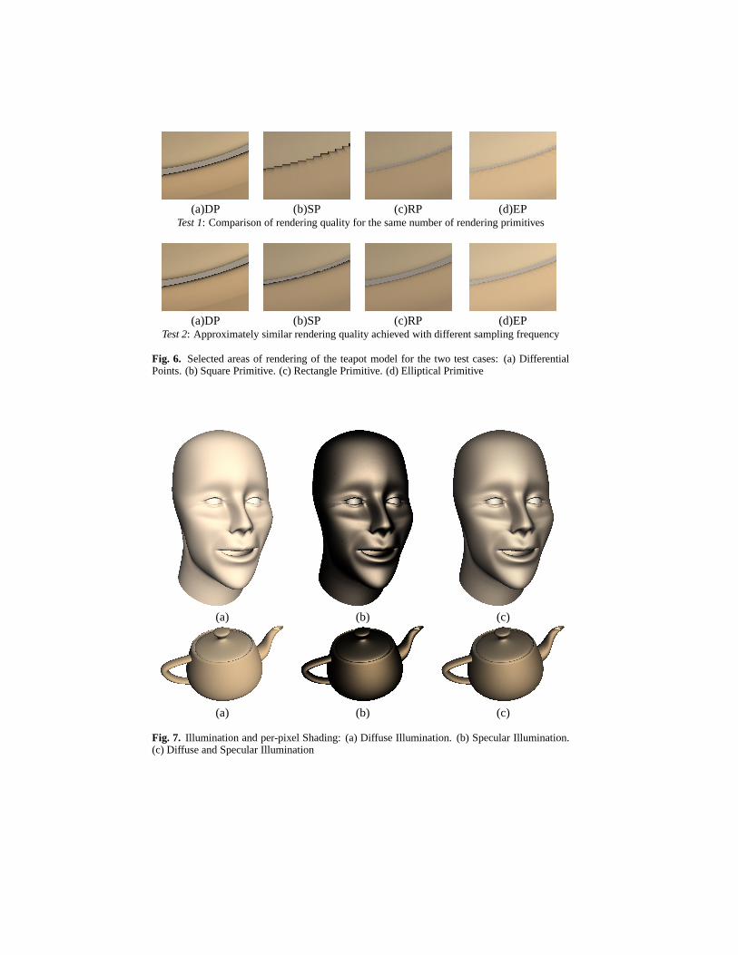
(a) (b) (c)

Fig. 4. Illumination and per-pixel Shading: (a) Diffuse Illumination. (b) Specular Illumination.(c) Diffuse and Specular Illumination

differential of equation (7) can then be re-written as follows:

@

@uHp(u; v)

����u=0

v=0

=@

@u

�Lp(u; v)

kLp(u; v)k+

Wp(u; v)

kWp(u; v)k

�����u=0

v=0

=((lp � up)lp � up)

ka� xpk+

((wp � up)wp � up)

kb� xpkWhen expressed in the local coordinate frame, we get:

@

@uHp(u; v)

����u=0

v=0

=((lp � ex)lp � ex)

ka� xpk+

((wp � ex)wp � ex)kb� xpk

(8)

the other partial differential of equation (7) can be computed similarly. The subtractionand the dot products in equation (8) are simple and fast operations. The square root andthe division operations are combined together by the fast inverse square root approxima-tion [16] which in practice causes no compromise in the visual quality. The light vectordistribution on�p can be derived similarly and is given bylp(u; v) � lp � uex � vey.

The tangent plane normal, half vector, and the light vector distribution aroundp areused for shadingp which essentially involves two kinds of computation: (1) mappingof the relevant vectors and (2) per-pixel computation. The overall rendering algorithmis given in Figure 5. The rectangler p is mapped by the normal map and the half vector(or light vector) map. Normal mapping involves choosing the best approximation to thenormal distribution from the set of pre-computed normal mapsM. Half-vector mappinginvolves computing un-normalized half vectors at the vertices ofr p using equation (7)and using them as the texture coordinates of the cube vector map that is mapped ontor p. Per-pixel shading is done in the hardware register combiners using the (per-pixel)normal and half vectors [10]. If both diffuse and specular shading are desired thenshading is done in two passes with the accumulation buffer being used to buffer theresults of the first pass. The accumulation buffer can be bypassed by disabling depthwrites in the second pass, but it leads to multiple writes to a pixel due to rectangleoverlaps and depth quantization which results in bright artifacts. If three textures areaccessible at the combiners then both illuminations can be combined into one pass.

6 Implementation and Results

All the test cases were run on a 866MHz Pentium 3 PC with 512MB RDRAM andhaving a nVIDIA GeForce2 card supported by 32MB of DDR RAM. All the test win-

Display( )(ComputeM and load them into texture memory at the program start time)

1 Clear the depth and the color buffers2 Configure the register combiners for diffuse shading3 8 DP p4 Mp = normal-map2M whose� is closest to�p5 MapMp ontor p6 Compute the light vector,lp(�; �), at the vertices ofr p7 Use the light vectors to map a cube vector map ontor p8 Renderr p9 Clear the color buffer after loading it into the accumulation buffer10 Clear the depth buffer11 Configure the register combiners for specular shading12 8 DP p13 Mp = normal-map2M whose� is closest to�p14 MapMp ontor p (The details from the last pass can be cached)15 Compute the half vector,hp(�; �), at the vertices ofr p16 Use the half vectors to map a cube vector map ontor p17 Renderr p18 Add the accumulation buffer to the color buffer19 Swap the front and the back color buffers

Fig. 5. The Rendering Algorithm

dows were 800�600 in size. We used 256 normal maps (jMj=256) corresponding touniformly sampled values of�p and we built a linear mip-map on each of these with ahighest resolution of 32�32. The resolution of the cube vector map was 512�512�6.

We demonstrate our work on three models: the Utah Teapot, a Human Head model,and a Camera prototype. The models are in the NURBS representation. The componentpatches are sampled uniformly in the parametric domain and simplified independentof each other. The error threshold� is the main parameter of the sampling process.Æ ensures that the rectangles from the low curvature region do not block the nearbyrectangles in the higher curvature regions and also ensures that the rectangles do notoverrun the boundary significantly. Simplification can lead to an order-of-magnitudespeed-up in rendering and can save substantial storage space as reported in Table 1. Inour current representation, each DP uses 62 bytes of storage: 6 bytes for the diffuseand specular colors, 12 floats (48 bytes) for the point location, principal directions andthe normal, and 2 floats (8 bytes) for the two curvature values. We anticipate over 80%compression by using quantized values, delta differences, and index colors. Both thespecular and diffuse shading are done at the hardware level. However, accumulationbuffer is not supported in hardware by nVIDIA and is implemented in software by theOpenGL drivers. So the case of both diffuse and specular illumination can be slow.

On an average, about330; 000 DPs can be rendered per second with diffuse illumi-nation. The diffuse and specular illumination passes take around the same time. Themain bottleneck in rendering is the bus bandwidth. This can be seen by noting thatspecular and diffuse illumination give around the same frame rates even though the costof computing the half vectors is higher than the cost of computing the light vectors andthat per-pixel computation is higher for specular illumination. The pixel-fill rate wasnot a bottleneck as the frame rates did not vary with the size of the window.

Table 1. Summary of results: NP = Number of points, SS = Storage Space, PT = Pre-processingtime, FPS = Frames per second. (Illumination is done with a moving light source)

Statistical Without Simplification With SimplificationHighlights Teapot Head Camera Teapot Head Camera

NP 156,800 376,400 216,712 25,713 64,042 46,077SS (in MB) 9.19 22.06 12.69 1.51 3.75 2.70PT (in sec) 22.5 22.2 15.25 146.5 485.5 178.17FPS (Diffuse) 2.13 0.89 1.59 12.51 5.26 6.89FPS (Specular) 2.04 0.88 1.52 11.76 5.13 6.67

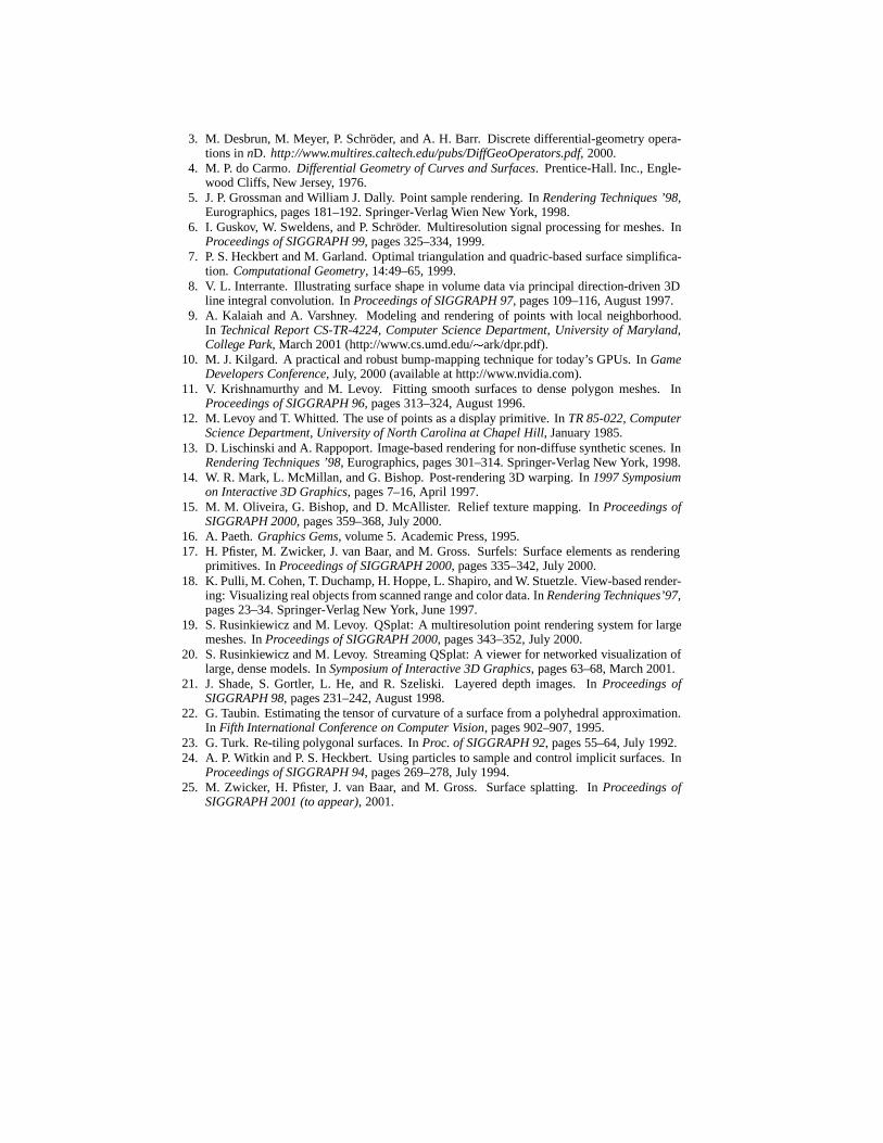
Table 2. Comparison with Splatting Primitives: (Test 1) Same Number of Rendering Primitives,(Test 2) Approximately similar rendering quality. DP = Differential Points, SP = Square Primi-tive, RP = Rectangle Primitive, and EP = Elliptical Primitive.

Rendering PrimitiveStatistical HighlightsDP SP RP EP

NP 156,800 156,800 156,800 156,800Test 1 SS (in MB) 9.19 4.90 4.90 4.90

FPS (Diffuse) 2.13 11.76 10.52 2.35NP 156,800 1,411,200 1,155,200 320,000

Test 2 SS (in MB) 9.19 44.10 36.10 10.01FPS (Diffuse) 2.13 1.61 1.49 1.16

The main focus of this paper is the rendering quality and efficiency delivered byDPs as rendering primitives. Previous works on point sample rendering have orthog-onal benefits such as faster transformation [21] and multiresolution [1, 17, 19] whichcan potentially be extended to DPs. To demonstrate the benefits of DPs we compare therendering performance of an unsimplified differential point representation of a teapot tothe splatting of unsimplified and unstructured versions of sampled points. For the splat-ting test cases, we take the original point samples from which DPs were constructedand associate each of them with a bounding ball whose radius is determined by com-paring its distance from its sampled neighbors. From this we consider three kinds oftest rendering primitives for splatting:

1. Square Primitive: They are squares parallel to the view plane with a width equalto the radius of the bounding ball [19]. They are rendered without blending.

2. Rectangle Primitive: Consider a disc on the tangent plane of the point, with aradius equal to the radius of the bounding ball. An orthogonal projection on a planeparallel to the view plane and located at the position of the point results in an ellipse.The rectangle primitive is obtained by fitting a rectangle around the ellipse with thesides of the rectangle being parallel to the principal axes of the ellipse [17]. Therectangle primitives are rendered with Z-buffering but without any blending.

3. Elliptical Primitive : We initialize 256 texture maps representing ellipses (with aunit radius along the semi-major axis) varying from a sphere to a nearly “flat” el-lipse. The texture maps have an alpha value of0 in the interior of the ellipse and1 elsewhere. At run time, the rectangle primitive is texture mapped with a scaledversion of the closest approximation of its ellipsoid. The texture-mapped rectanglesare then rendered with a small depth offset and blending [19]. This is implementedin hardware using the register combiners.

DPs were compared with the splatting primitives for two test cases: (Test 1) samenumber of rendering primitives and (Test 2) approximately similar visual quality of ren-dering. ForTest 1, DPs were found to deliver a much better rendering quality for thesame number of primitives as seen in Figure 6 and summarized in Table 2. DPs espe-cially fared well in high curvature areas which are not well modeled and rendered by thesplat primitives. Moreover, DPs had nearly the same frame rates as the elliptical primi-tives. Sample renderings ofTest 2are shown in Figure 6 and the results are summarizedin Table 2. For this test the number of square, rectangle, and elliptical primitives wereincreased by increasing the sampling frequency of the uniformly sampled model usedfor DPs. InTest 2, DPs clearly out-performed the splatting primitives in both criteria.

7 Conclusions and Future Work

The results and the test comparisons clearly demonstrate the efficiency of DPs as ren-dering primitives. The ease of simplification gives DPs an added advantage to get asignificant speed up. High rendering quality is achieved because the normal distribu-tion is fairly accurate. The rendering efficiency of DPs is attributed to the sparse surfacerepresentation that reduces bus bandwidth.

One shortcoming of DPs is that the complexity of the borders limit the maximumwidth of the interior DPs through theÆ constraint. This leads to increased samplingin the interior even though these DPs have enough room to expand within the boundslaid down by the� constraint. A width-determination approach that uses third orderdifferential information (such as the variation of the surface curvature) should be ableto deal with this more efficiently. DPs are currently implemented for a NURBS rep-resentation. The main challenge in extending them to polygonal models would be theaccurate computation of curvature properties and handling of discontinuities.

In its current form DPs are not efficient when a large set of points fall onto the samepixel while rendering. We plan to explore a multiresolution scheme of DPs that willefficiently render lower frequency versions of the original surface under such instances.Texturing can be achieved by texturing the rectanglesr p and having a separate texturepass while rendering. The texture coordinates of the vertices ofr p can be computedwith the aid of the object space parameterization ofSp.

8 Acknowledgements

We would like to thank the anonymous reviewers for their constructive comments thatwere exceptionally detailed and insightful. We would like to thank our colleagues atthe Graphics and Visual Informatics Laboratory at the University of Maryland, CollegePark and at the Center for Visual Computing at SUNY, Stony Brook. We would alsolike to thank Robert McNeel & Associates for the Head and the Camera models and forthe openNURBS C++ code. Last, but not the least, we would like to acknowledge NSFfunding grants IIS00-81847, ACR-98-12572 and DMI-98-00690.

References

1. C. F. Chang, G. Bishop, and A. Lastra. LDI Tree: A hierarchical representation for image-based rendering. InProceedings of SIGGRAPH’99, pages 291–298, 1999.

2. L. Darsa, B. C. Silva, and A. Varshney. Navigating static environments using image-spacesimplification and morphing. In1997 Symp. on Interactive 3D Graphics, pages 25–34, 1997.

3. M. Desbrun, M. Meyer, P. Schr¨oder, and A. H. Barr. Discrete differential-geometry opera-tions innD. http://www.multires.caltech.edu/pubs/DiffGeoOperators.pdf, 2000.

4. M. P. do Carmo.Differential Geometry of Curves and Surfaces. Prentice-Hall. Inc., Engle-wood Cliffs, New Jersey, 1976.

5. J. P. Grossman and William J. Dally. Point sample rendering. InRendering Techniques ’98,Eurographics, pages 181–192. Springer-Verlag Wien New York, 1998.

6. I. Guskov, W. Sweldens, and P. Schr¨oder. Multiresolution signal processing for meshes. InProceedings of SIGGRAPH 99, pages 325–334, 1999.

7. P. S. Heckbert and M. Garland. Optimal triangulation and quadric-based surface simplifica-tion. Computational Geometry, 14:49–65, 1999.

8. V. L. Interrante. Illustrating surface shape in volume data via principal direction-driven 3Dline integral convolution. InProceedings of SIGGRAPH 97, pages 109–116, August 1997.

9. A. Kalaiah and A. Varshney. Modeling and rendering of points with local neighborhood.In Technical Report CS-TR-4224, Computer Science Department, University of Maryland,College Park, March 2001 (http://www.cs.umd.edu/�ark/dpr.pdf).

10. M. J. Kilgard. A practical and robust bump-mapping technique for today’s GPUs. InGameDevelopers Conference, July, 2000 (available at http://www.nvidia.com).

11. V. Krishnamurthy and M. Levoy. Fitting smooth surfaces to dense polygon meshes. InProceedings of SIGGRAPH 96, pages 313–324, August 1996.

12. M. Levoy and T. Whitted. The use of points as a display primitive. InTR 85-022, ComputerScience Department, University of North Carolina at Chapel Hill, January 1985.

13. D. Lischinski and A. Rappoport. Image-based rendering for non-diffuse synthetic scenes. InRendering Techniques ’98, Eurographics, pages 301–314. Springer-Verlag New York, 1998.

14. W. R. Mark, L. McMillan, and G. Bishop. Post-rendering 3D warping. In1997 Symposiumon Interactive 3D Graphics, pages 7–16, April 1997.

15. M. M. Oliveira, G. Bishop, and D. McAllister. Relief texture mapping. InProceedings ofSIGGRAPH 2000, pages 359–368, July 2000.

16. A. Paeth.Graphics Gems, volume 5. Academic Press, 1995.17. H. Pfister, M. Zwicker, J. van Baar, and M. Gross. Surfels: Surface elements as rendering

primitives. InProceedings of SIGGRAPH 2000, pages 335–342, July 2000.18. K. Pulli, M. Cohen, T. Duchamp, H. Hoppe, L. Shapiro, and W. Stuetzle. View-based render-

ing: Visualizing real objects from scanned range and color data. InRendering Techniques’97,pages 23–34. Springer-Verlag New York, June 1997.

19. S. Rusinkiewicz and M. Levoy. QSplat: A multiresolution point rendering system for largemeshes. InProceedings of SIGGRAPH 2000, pages 343–352, July 2000.

20. S. Rusinkiewicz and M. Levoy. Streaming QSplat: A viewer for networked visualization oflarge, dense models. InSymposium of Interactive 3D Graphics, pages 63–68, March 2001.

21. J. Shade, S. Gortler, L. He, and R. Szeliski. Layered depth images. InProceedings ofSIGGRAPH 98, pages 231–242, August 1998.

22. G. Taubin. Estimating the tensor of curvature of a surface from a polyhedral approximation.In Fifth International Conference on Computer Vision, pages 902–907, 1995.

23. G. Turk. Re-tiling polygonal surfaces. InProc. of SIGGRAPH 92, pages 55–64, July 1992.24. A. P. Witkin and P. S. Heckbert. Using particles to sample and control implicit surfaces. In

Proceedings of SIGGRAPH 94, pages 269–278, July 1994.25. M. Zwicker, H. Pfister, J. van Baar, and M. Gross. Surface splatting. InProceedings of

SIGGRAPH 2001 (to appear), 2001.

(a)DP (b)SP (c)RP (d)EPTest 1: Comparison of rendering quality for the same number of rendering primitives

(a)DP (b)SP (c)RP (d)EPTest 2: Approximately similar rendering quality achieved with different sampling frequency

Fig. 6. Selected areas of rendering of the teapot model for the two test cases: (a) DifferentialPoints. (b) Square Primitive. (c) Rectangle Primitive. (d) Elliptical Primitive

(a) (b) (c)

(a) (b) (c)

Fig. 7. Illumination and per-pixel Shading: (a) Diffuse Illumination. (b) Specular Illumination.(c) Diffuse and Specular Illumination