Takustraße 7D-14195 Berlin-Dahlem

GermanyKonrad-Zuse-Zentrumfur Informationstechnik Berlin

P. DEUFLHARD

Differential Equations in Technology andMedicine. Computational Concepts, Adaptive

Algorithms, and Virtual Labs.

Preprint SC 99–34 (September 1999)

Differential Equations in Technology and Medicine.

Computational Concepts, Adaptive Algorithms,

and Virtual Labs.

CIME Lectures

Peter Deuflhard

Abstract

This series of lectures has been given to a class of mathematics postdocs at aEuropean summer school on Computational Mathematics Driven by Indus-trial Applications in Martina Franca, Italy (organized by CIME). It dealswith a variety of challenging real life problems selected from clinical cancertherapy, communication technology, polymer production, and pharmaceu-tical drug design. All of these problems from rather diverse applicationareas share two common features: (a) they have been modelled by variousdifferential equations – elliptic, parabolic, or Schrodinger–type partial differ-ential equations, countable ordinary differential equations, or Hamiltoniansystems, (b) their numerical solution has turned out to be a real challengeto computational mathematics.

Contents

Introduction 1

1 Partial Differential Equations in Cancer Therapy Planning 2

1.1 Multilevel Finite Element Methods Revisited . . . . . . . . . . . . . 2

1.2 Clinical Therapy Planning by Virtual Patients . . . . . . . . . . . . 8

2 Partial Differential Equations in Optical Chip Design 16

2.1 Beam Propagation Analysis . . . . . . . . . . . . . . . . . . . . . . 17

2.2 Guided Mode Analysis . . . . . . . . . . . . . . . . . . . . . . . . . 20

3 Countable Ordinary Differential Equations in Polymer Industry 26

3.1 Polyreaction Kinetics . . . . . . . . . . . . . . . . . . . . . . . . . . 26

3.2 Basic Computational Approaches . . . . . . . . . . . . . . . . . . . 29

3.3 Adaptive Discrete Galerkin Methods . . . . . . . . . . . . . . . . . 32

4 Hamiltonian Equations in Pharmaceutical Drug Design 38

4.1 Deterministic Chaos in Molecular Dynamics . . . . . . . . . . . . . 39

4.2 Identification of Metastable Conformations . . . . . . . . . . . . . . 44

4.3 Virtual RNA Lab . . . . . . . . . . . . . . . . . . . . . . . . . . . . 49

References 53

Introduction

This series of lectures has been given to a class of mathematics postdocs at aEuropean summer school in Martina Franca (organized by CIME). It deals witha variety of challenging real life problems selected from clinical cancer therapy,communication technology, polymer production, and pharmaceutical drug design.All of these problems from rather diverse application areas share two commonfeatures: (a) they have been modelled by various differential equations – elliptic,parabolic, or Schrodinger–type partial differential equations, countable ordinarydifferential equations, or Hamiltonian systems, (b) their numerical solution hasturned out to be a real challenge to computational mathematics.

Therefore, before diving into actual computation, the computational concepts to beapplied need to be carefully considered. To start with, any numerical analyst mustbe prepared to totally remodel problems coming from science or engineering – seee.g. Sections 3 and 4 below. The computational problems to be treated shouldbe well–posed, important features of any underlying continuous model should bepassed on, if at all possible, to the discrete model, and the computational resourcesemployed (computing time, storage, graphics) should be adequate.

Speaking in mathematical terms, the solutions to be approximated live in appro-priate infinite dimensional function spaces, e.g. in Sobolev spaces in Sections 1and 2, in discrete weighted sequence spaces in Section 3, or in certain statisticallyweighted function spaces in Section 4. The mathematical paradigm advocatedthroughout this paper is that – already due to mathematical aesthetics – any infi-nite dimensional space should not be represented by just a single finite dimensionalspace (with possibly large dimension), but by a well–designed sequence of finitedimensional spaces, which successively exploit the asymptotic properties charac-terizing the original function space. The fascinating, but (for a mathematician)not really surprising experience is that mathematical aesthetics go directly withcomputational efficiency. In other words, a careful and sufficiently ingenious real-ization of the above paradigm will lead to efficient algorithms that actually workin hard real life problems. The reason for this coincidence of aesthetics and ef-ficiency lies in the fact that function spaces describe some data redundancy thatcan be exploited in the numerical solution process. In order to do so, adaptivity ofalgorithms is one of the leading construction principles. Typically, wherever adap-tivity has been successfully realized, algorithms with a computational complexityclose to the (unavoidable) complexity of the problem emerge – a feature of extremeimportance especially in challenging problems of science, technology, or medicine.

1

In traditional industrial environments, however, new efficient mathematical algo-rithms are not automatically accepted – even if they significantly supercede alreadyexisting older ones (if not old–fashioned ones) within long established commercialsoftware systems. Exceptions do occur where simulation or optimization is thedominating competition factor. Due to this experience the author’s group has puta lot of effort in the design of virtual labs. These specialized integrated softwaresystems permit a fast and convenient switch between numerical code and interac-tive visualization tools (that we also develop, but do not touch here). Sometimesonly such virtual labs open the door for new mathematical ideas in hospitals orindustrial labs.

1 Partial Differential Equations in Cancer

Therapy Planning

The present section deals with partial differential equation (PDE) models arisingin medicine (example: cancer therapy hyperthermia) and high frequency electri-cal engineering (example: radio wave absorption). In this type of application the3D geometry – say, of human patients – motivates the choice of tetrahedral finiteelement methods (FEM). The clinical setting requires the robust computationalsolution of problems to prescribed accuracy at highest possible speed on localworkstations. Reliability plays the dominant role in medicine, which is a nice par-allelism with the intentions of mathematics. Numerical speed is required to permita fast simulation of different scenarios for different patients. In other words: thesituation both requires and deserves the construction of highly efficient algorithms,numerical software, and visualization tools.

1.1 Multilevel Finite Element Methods Revisited

The presentation of this section focusses on elliptic or parabolic PDEs and Maxwell’sequations. Mathematically speaking, the stationary solutions of these PDEs livein some Sobolev space like Hα or Hcurl depending on the prescribed boundary con-ditions, whereas the time dependent solutions live in some scale of these spaces.In view of the above mentioned paradigm and the expected computational com-plexity, these spaces are approximated by a sequence of finite element spaces inthe frame of multigrid (MG) or multilevel (ML) methods. Before going into thetechnical details of the real life problems to be presented below, a roadmap ofseveral advanced computational concepts will be given first that have turned out

2

to be important not only for the herein selected applications.

Optimal multigrid complexity. Classical MG methods have been first ad-vocated for actual computation in the 70’s by A. Brandt [26] and Hackbusch

[52]. The latter author has paved the success path for MG methods by first provingan optimal computational complexity estimate O(N) for the so–called W–cycle,where N was understood to be the number of nodes in a uniform space grid. Thesame attractive feature was observed in suitable implementations of the simplerV–cycle and later proved by Braess and Hackbusch[23] under certain regu-larity assumptions and for uniform grids. The subsequent development was thencharacterized by a successive extension of MG methods from the originally onlyelliptic problems to larger and larger problem classes.

Adaptive multilevel methods. In quite a number of industrially relevant prob-lems rather localized phenomena occur. In this case, uniform grids are by nomeans optimal, which, in turn, also means that the classical MG methods on uni-form grids could not be regarded as optimal. For this reason, multigrid methodson adaptive grids have been developed quite early, probably first by R. Bank [8]in his code PLTMG in the context of problems arising from semiconductor devicemodelling where sharp local boundary layers arise naturally. Later adaptive MGimplementations are the code family KASKADE [14] by the author’s group andthe code family UG [11] by Wittum, Bastian, and co-workers. UG in partic-ular pays careful attention to parallelization issues [12]. The proof of an optimalcomputational complexity estimate O(Nad), where Nad is now understood to bethe often much smaller adaptive number of nodes, turned out to need more so-phisticated proof techniques; for the well–known V–cycle, this challenging task hasbeen performed by Bramble, Pasciak, Wang, and Xu [25] – see also Xu [90].His rather elegant theoretical tools came from the interpretation of MG methodsas abstract multiplicative Schwarz methods (equivalent to abstract Gauss–Seidelmethods) based on an underlying multilevel splitting in function space.

Hierarchical bases finite element methods. Independent of the classicalMG methods, a novel multilevel method based on conjugate gradient iteration withsome hierarchical basis (HB) preconditioning had been suggested in the mid 80’s forelliptic PDEs by Yserentant [91]. From the scratch, this new type of algorithmturned out to be competitive with classical MG in terms of computational speed.An adaptive 2D version of the new method had been designed and implementedin the late 80’s by Deuflhard, Leinen, and Yserentant [39] in the code

3

KASKADE. On top of that first realization, a more mature version including also3D has been worked out by Bornemann, Erdmann, and Kornhuber [16].The present version of KASKADE [14] contains the original HB–preconditioner for2D and the more recent BPX–preconditioner due to Xu [89, 24] for 3D. For anaccount of its performance see Section 1.2.

Additive versus multiplicative multigrid methods. After the theoreticalmilestone paper by Xu [90], the hierarchical basis type methods are now inter-preted as abstract additive Schwarz methods (equivalent to abstract Jacobi meth-ods) also based on a multilevel decomposition in function space. By constructionadditive Schwarz methods provide some preconditioning. In this interpretation,which the author prefers to adopt, the classical multigrid methods are then calledmultiplicative MG methods, whereas the HB– or BPX–preconditioned CG methodsare called additive MG methods. In particular, the BPX–preconditioning and theV–cycle are just the additive and multiplicative counterparts. From theoreticalanalysis, multiplicative MG methods might require less iterations – which, how-ever, need not imply less computing time (see e.g. the Maxwell MG solvers inSection 1.2 below, Table 1.1). Moreover, if an additive MG involves only one iter-ation on the finest grid, then multiplicative MG methods cannot gain too much. Inthe subsequently described elliptic problems, the bulk of computing time is anywayspent in the evaluation of the stiffness matrix elements and the right hand sideelements. Summarizing, the question of whether additive or multiplicative MGmethods should be preferred, appears to be less important than other conceptualissues – see below. For the orientation of the reader: UG is strictly multiplica-tive, PLTMG is dominantly multiplicative with some additive options, KASKADEis dominantly additive with some multiplicative code e.g. for eigenvalue problemsand the harmonic Maxwell’s equations. A common software platform of UG andKASKADE is in preparation.

Cascadic multigrid methods. These rather recent MG methods can be un-derstood as some confluence of additive and multiplicative MG methods. Fromthe additive point of view, cascadic multigrid (CMG) methods are characterizedby the simplest possible preconditioner: either no or just a diagonal preconditioneris applied; as a distinguishing feature, coarser levels are visited more often thanfiner levels – to serve as preconditioning substitutes. From the multiplicative side,CMG methods may be understood as MG methods with an increased number ofsmoothing iterations on coarser levels, but without any coarse grid corrections. Asa first algorithm of this type, a cascadic conjugate gradient method (CCG) had beenproposed by the author in [30]. The general CMG class with arbitrary smoothers

4

beyond CG has been presented by Bornemann and Deuflhard [20]. In theirpaper they analyzed CMG in terms of convergence and computational complexityin an adaptive setting – based on first much more restrictive convergence resultsdue to Shaidurov [82]. These CMG methods exhibit good convergence propertiesonly in H1, but not in L2 – unlike additive (with appropriate preconditioning) ormultiplicative MG methods. Therefore, though being certainly easiest to imple-ment among all MG methods, CMG methods – the youngest members of the MGfamily – are still in the process of maturing. Just to avoid mixing terms: CMGis different from the code KASKADE, which predominantly realizes additive MGmethods.

Local error estimators. Any efficient implementation of adaptive MG methods(additive, multiplicative, cascadic) must be based on cheap local error estimatorsor, at least, local error indicators. In the best case, these are derived from the-oretical a–posteriori error estimates. These estimates will be local only, if local(right hand side) perturbations in the given problem remain local – i.e. if theGreens’ function of the PDE problem exhibits local behavior. As a consequenceof this elementary insight, adaptive MG methods will be essentially applicable tolinear or nonlinear elliptic or parabolic problems. As for a comparative assess-ment of the different available local error estimators, there is a beautiful paper byBornemann, Erdmann, and Kornhuber [17] that gives a unified theoreticalframework for most of the popular 2D and 3D error estimators. For orientation:PLTMG uses the triangle oriented estimator of Bank and Weiser [10], KASKADEthe edge oriented estimator of Deuflhard, Leinen, Yserentant, and UG theestimator of Babuska and Miller [4].

Adaptive grid refinement. Within adaptive ML methods simplicial grids playa dominant role, since they behave nicely in local refinement processes. In con-nection with any selected error estimator, the local extrapolation method due toBabuska and Rheinboldt [5] can be applied to determine some threshold value,above which a geometrical element (tetrahedron, triangle, edge) is marked for localrefinement. Once this marking has been done, well–designed strategies need to beapplied to produce a complete FE grid on the next refinement level. The art ofrefinement is quite established in 2D (see the “red” and “green” refinements dueto Bank et al. [9] or the “blue” refinement due to Kornhuber and Roitzsch

[62]). In 3D there is still work left to be done, even though successful strategiesdue to Rivara[73], Ong[71], or Bey[15] have been around for quite a time.

5

Multilevel methods for nonlinear elliptic problems. For nonlinear ellipticproblems there are two basic lines of MG methods: (I) the nonlinear MG method,sometimes also called full approximation scheme (FAS), wherein nonlinear resid-uals are evaluated within MG cycles, and (II) the Newton MG method, whereinlinear residuals are evaluated within the MG method for the solution of the lin-ear systems for the Newton corrections. In [42, 44] Deuflhard and Weiser

proposed an adaptive version for the second MG approach based on an affineconjugate characterization of nonlinearity via the special Lipschitz condition

‖F ′(x)−1/2(F ′(y) − F ′(x)

)(y − x)‖ ≤ ω‖F ′(x)1/2(y − x)‖. (1.1)

This type of condition enters into certain affine invariant convergence results forboth local and global inexact Newton methods in the function spaces W p,q. Theassociated code Newton–KASKADE realizes a theoretically backed optimal balancebetween outer Newton iterations with possible adaptive damping, multilevel dis-cretization, and inner preconditioned CG iterations; its performance is exemplifiedin Section 1.2 below.

Method of lines for parabolic PDEs. For time dependent PDEs, the mostpopular approach is still the so–called method of lines (MOL), which realizes afirst space / then time discretization. After space discretization a typically largeblock–structured system of ordinary differential equations (ODEs) arises, which isthen solved by any stiff ODE integrator: in the simplest (but often inefficient) caseby an implicit or backward Euler with constant timestep, in advanced versions bysome implicit multistep code (like DASSL), some implicit Runge–Kutta code (likeRADAU 5), or some linearly implicit extrapolation code (like LIMEX) with adaptivecontrol of timestep and possibly time discretization order. However, if one aims atdynamically adapted non–uniform space grids in 2D or 3D with MG methods tobe applied, which is the typical case in parabolic PDEs, then the MOL approachwill lead into some mass.

Adaptive Rothe method for linear parabolic PDEs. Starting 91, Borne-

mann [18, 19] suggested to abandon the MOL for parabolic PDEs and to usethe so–called Rothe method instead, which realizes a first time / then space dis-cretization. His first papers dealt with initial boundary value problems for linearscalar parabolic PDEs such as

ut = −Δu + f(x), u(x, 0) = ϕ(x), u(x, t) |∂Ω= ψ(t), t ≥ 0, x ∈ Ω ⊂ Rd . (1.2)

6

Upon incorporating the boundary conditions into a linear elliptic operator A somefunction U is defined by virtue of the abstract Cauchy problem

U ′(t) = AU + F, U(0) = U0 . (1.3)

Note that U represents a spatial function living in some scale of Hilbert spacesHα(Ω). The above abstract ordinary differential equation (ODE) may now beformally discretized for time step τ by some stiff integration scheme. For simplicity,we choose the implicit Euler method, which generates an equation of the type

(I − τA)ΔU = τF . (1.4)

This equation represents some (τ–dependent) elliptic boundary value problem,which can be solved by any adaptive multilevel method. Moreover, the availableadvanced ODE technology may also enter, but now in function space – which meansthat any error control devices known from finite dimensional ODEs are realizedvia spatial approximations using an adaptive MLFEM. Summarizing, a substantialadvantage of this reversed order of discretization turns out to be that dynamicspace grid adaptation and adaptive MG methods within each time layer are, inprinciple, easy to apply. Moreover, this approach nicely reflects the underlyingtheoretical structure.

Adaptive Rothe method for nonlinear parabolic PDEs. The above algo-rithmic approach can be extended to the nonlinear parabolic case. A rather directextension is obtained on the basis of some abstract stiffness theory presented bythe author in [31]. In this paper stiff time discretization of a nonlinear ODE initialvalue problem, say

U ′ = F (U), U(0) = U0 (1.5)

has been interpreted as a simplified Newton iteration for the evolution problem infunction space. This Newton iteration, in turn, may be formally understood as aPicard iteration for the slightly rewritten ODE

U ′ −AU = F (U) −AU, U(0) = U0 (1.6)

wherein A ≈ F ′(U0) – i.e. in finite dimension A is just an approximate Jaco-bian (n, n)–matrix of the right hand side. From this theoretical insight linearlyimplicit stiff integration methods appear naturally – as opposed to nonlinear stiffdiscretization schemes like BDF or implicit RK methods. The concept directlycarries over to infinite dimension when equations (1.5) and (1.6) are any abstract

7

Cauchy problem. Upon applying, for simplicity, the linearly implicit Euler dis-cretization to (1.5), we arrive at some linear boundary value problem of the kind

(I − τA)ΔU = τ(F (U) −AU

). (1.7)

Following this line, Lang [63, 64] developed the adaptive multilevel code KAR-DOS that realizes a linearly implicit (embedded) Runge–Kutta method of low orderon each discretization level. In its present form, this most recent code from theKASKADE family is applicable to 3D nonlinear systems of reaction–diffusion equa-tions with mild convection. Generally speaking, since the adaptive Rothe methodis fully adaptive in both time and space, it is able to resolve extreme multiscalesin time and space that often arise in hard real life problems – like e.g. in chemicalcombustion. An early comparison of the new approach with the more traditionalMOL approach (both adaptive 1D implementations) can be found in the surveypaper [38]. The Rothe method will play a role in Section 1.2, Section 2, andSection 3.

1.2 Clinical Therapy Planning by Virtual Patients

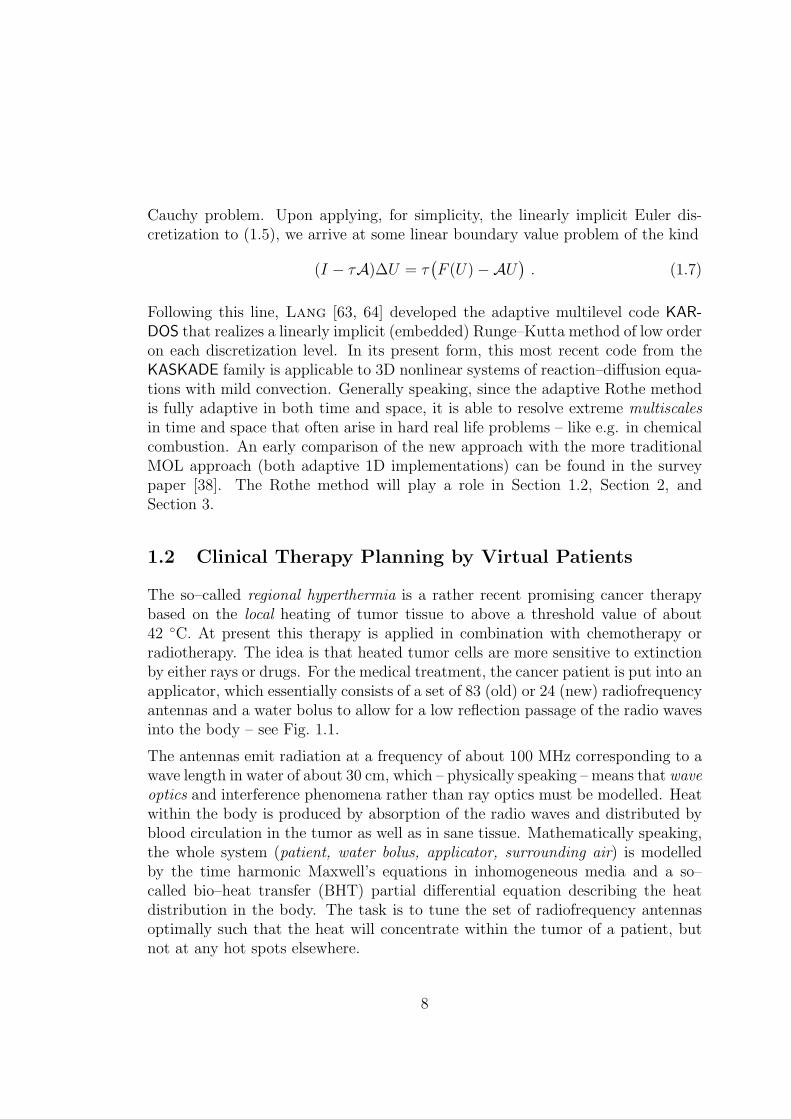
The so–called regional hyperthermia is a rather recent promising cancer therapybased on the local heating of tumor tissue to above a threshold value of about42 ◦C. At present this therapy is applied in combination with chemotherapy orradiotherapy. The idea is that heated tumor cells are more sensitive to extinctionby either rays or drugs. For the medical treatment, the cancer patient is put into anapplicator, which essentially consists of a set of 83 (old) or 24 (new) radiofrequencyantennas and a water bolus to allow for a low reflection passage of the radio wavesinto the body – see Fig. 1.1.

The antennas emit radiation at a frequency of about 100 MHz corresponding to awave length in water of about 30 cm, which – physically speaking – means that waveoptics and interference phenomena rather than ray optics must be modelled. Heatwithin the body is produced by absorption of the radio waves and distributed byblood circulation in the tumor as well as in sane tissue. Mathematically speaking,the whole system (patient, water bolus, applicator, surrounding air) is modelledby the time harmonic Maxwell’s equations in inhomogeneous media and a so–called bio–heat transfer (BHT) partial differential equation describing the heatdistribution in the body. The task is to tune the set of radiofrequency antennasoptimally such that the heat will concentrate within the tumor of a patient, butnot at any hot spots elsewhere.

8

Figure 1.1: Real patient in hospital (Sigma–60 applicator).

In the project to be reported here, we have been collaborating with internationallyrenowned oncologists at one of the large Berlin hospitals, the Rudolf–Virchow–Klinikum at the Charite of the Humboldt University. Our task is to support thepatient–specific planning of individual therapies. In order to make the method atall useful in a clinical environment, the computational results must be obtainedwithin hours (at most) on a workstation in hospital to medical reliability. In ad-dition, any numerical results are to be presented in visual form so that they canbe directly interpreted and conveniently handled by medical staff. These require-ments made the development of an integrated software package necessary thatcombines efficient 3D interaction tools with both numerical and computer graph-ical algorithms. As a prerequisite for the PDE solvers, a rather detailed virtualpatient needs to be built up from medical imaging input (at present computedtomograms). The system as it stands now is already able to decide about thequestion whether a given patient can be expected to be successfully treated byhyperthermia using a given applicator. The presentation herein essentially followsthe articles [41, 40]

Electric field simulation. We model the antennas by a fixed (angular) fre-quency ω and the human tissues so that Ohm’s law holds. Let the electric fieldhave a representation of the form ReE(x)eiωt with a complex amplitude E(x) de-fined on a computational domain Ω ⊂ R3. Then the time harmonic Maxwell’s

9

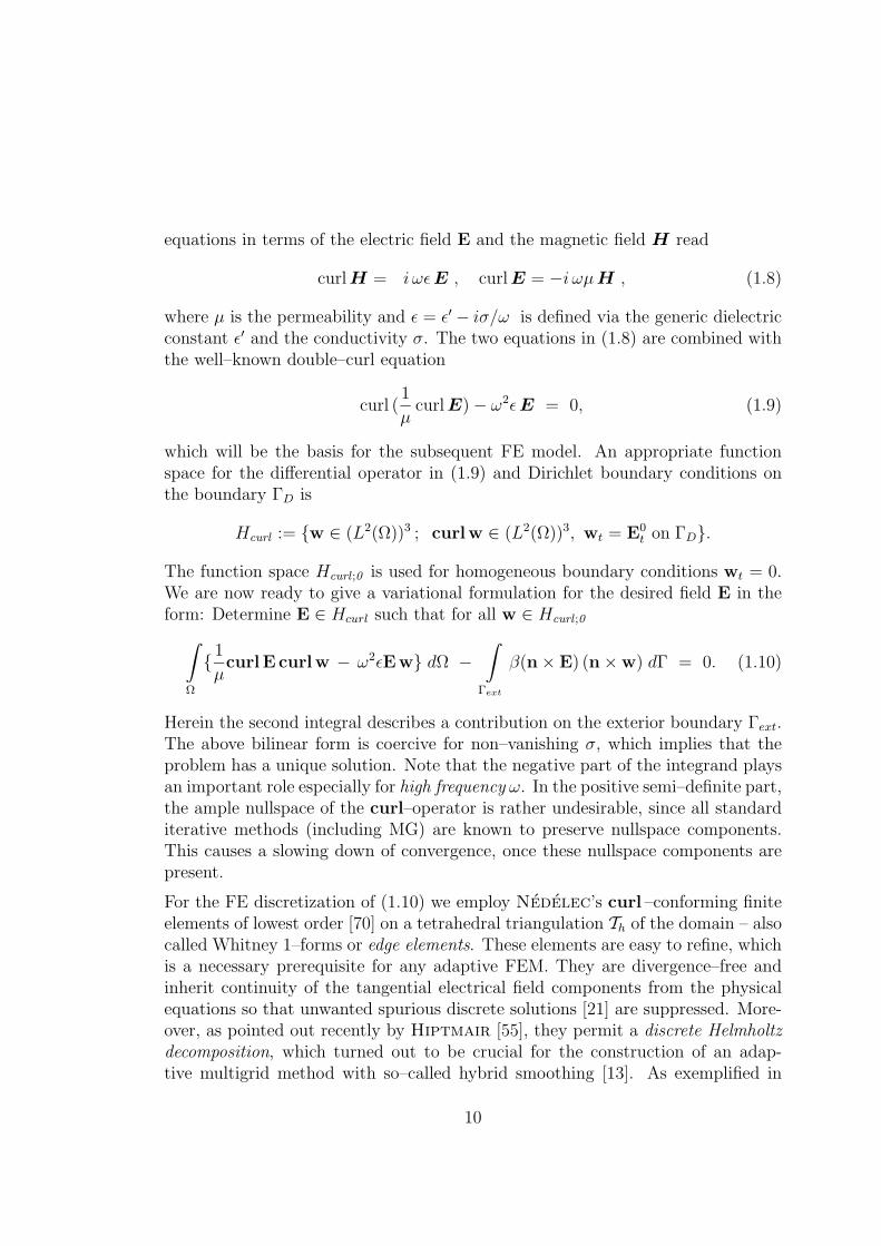
equations in terms of the electric field E and the magnetic field H read

curl H = i ωε E , curl E = −i ωμH , (1.8)

where μ is the permeability and ε = ε′ − iσ/ω is defined via the generic dielectricconstant ε′ and the conductivity σ. The two equations in (1.8) are combined withthe well–known double–curl equation

curl (1

μcurl E) − ω2ε E = 0, (1.9)

which will be the basis for the subsequent FE model. An appropriate functionspace for the differential operator in (1.9) and Dirichlet boundary conditions onthe boundary ΓD is

Hcurl := {w ∈ (L2(Ω))3 ; curlw ∈ (L2(Ω))3, wt = E0t on ΓD}.

The function space Hcurl ;0 is used for homogeneous boundary conditions wt = 0.We are now ready to give a variational formulation for the desired field E in theform: Determine E ∈ Hcurl such that for all w ∈ Hcurl ;0∫

Ω

{ 1

μcurlE curlw − ω2εEw} dΩ −

∫Γext

β(n × E) (n × w) dΓ = 0. (1.10)

Herein the second integral describes a contribution on the exterior boundary Γext.The above bilinear form is coercive for non–vanishing σ, which implies that theproblem has a unique solution. Note that the negative part of the integrand playsan important role especially for high frequency ω. In the positive semi–definite part,the ample nullspace of the curl–operator is rather undesirable, since all standarditerative methods (including MG) are known to preserve nullspace components.This causes a slowing down of convergence, once these nullspace components arepresent.

For the FE discretization of (1.10) we employ Nedelec’s curl –conforming finiteelements of lowest order [70] on a tetrahedral triangulation Th of the domain – alsocalled Whitney 1–forms or edge elements. These elements are easy to refine, whichis a necessary prerequisite for any adaptive FEM. They are divergence–free andinherit continuity of the tangential electrical field components from the physicalequations so that unwanted spurious discrete solutions [21] are suppressed. More-over, as pointed out recently by Hiptmair [55], they permit a discrete Helmholtzdecomposition, which turned out to be crucial for the construction of an adap-tive multigrid method with so–called hybrid smoothing [13]. As exemplified in

10

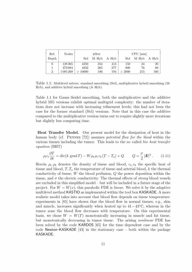
Ref. Nodes #Iter CPU [min]Depth Std M–Hyb A–Hyb Std M–Hyb A–Hyb

0 128 365 4250 354 413 150 24 201 373 084 4832 265 277 800 76 602 1 085 269 > 10000 186 194 > 2000 215 160

Table 1.1: Multilevel solvers: standard smoothing (Std), multiplicative hybrid smoothing (M-Hyb), and additive hybrid smoothing (A–Hyb).

Table 1.1 for Gauss–Seidel smoothing, both the multiplicative and the additivehybrid MG versions exhibit optimal multigrid complexity: the number of itera-tions does not increase with increasing refinement levels; this had not been thecase for the former standard (Std) versions. Note that in this case the additivecompared to the multiplicative version turns out to require slightly more iterationsbut slightly less computing time.

Heat Transfer Model. Our present model for the dissipation of heat in thehuman body (cf. Pennes [72]) assumes potential flow for the blood within thevarious tissues including the tumor. This leads to the so–called bio–heat transferequation (BHT)

ρtct∂T

∂t= div(k grad T ) − Wρb ρt cb (T − Ta) + Q Q =

σ

2|E|2 . (1.11)

Herein ρt, ρb denotes the density of tissue and blood, ct, cb the specific heat oftissue and blood, T, Ta the temperature of tissue and arterial blood, k the thermalconductivity of tissue, W the blood perfusion, Q the power deposition within thetissue, and σ the electric conductivity. The thermal effects of strong blood vesselsare excluded in this simplified model – but will be included in a future stage of theproject. For W = W (x), this parabolic PDE is linear. We solve it by the adaptivemultilevel method KASTIO as implemented within the tool box KASKADE. A morerealistic model takes into account that blood flow depends on tissue temperature:experiments in [85] have shown that the blood flow in normal tissues, e.g., skinand muscle, increases significantly when heated up to 41−43◦C, whereas in thetumor zone the blood flow decreases with temperature. On this experimentalbasis, we chose W = W (T ) monotonically increasing in muscle and fat tissue,but monotonically decreasing in tumor tissue. The arising nonlinear PDE hasbeen solved by the code KARDOS [65] for the time dependent case and by thecode Newton–KASKADE [43] in the stationary case – both within the packageKASKADE.

11

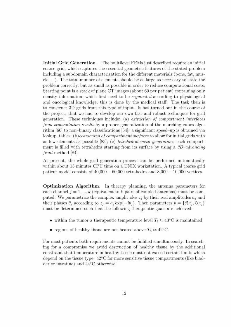
Initial Grid Generation. The multilevel FEMs just described require an initialcoarse grid, which captures the essential geometric features of the stated problemincluding a subdomain characterization for the different materials (bone, fat, mus-cle, ...). The total number of elements should be as large as necessary to state theproblem correctly, but as small as possible in order to reduce computational costs.Starting point is a stack of plane CT images (about 60 per patient) containing onlydensity information, which first need to be segmented according to physiologicaland oncological knowledge; this is done by the medical staff. The task then isto construct 3D grids from this type of input. It has turned out in the course ofthe project, that we had to develop our own fast and robust techniques for gridgeneration. These techniques include: (a) extraction of compartment interfacesfrom segmentation results by a proper generalization of the marching cubes algo-rithm [66] to non–binary classifications [54]: a significant speed–up is obtained vialookup–tables; (b)coarsening of compartment surfaces to allow for initial grids withas few elements as possible [83]; (c) tetrahedral mesh generation: each compart-ment is filled with tetrahedra starting from its surface by using a 3D–advancingfront method [84].

At present, the whole grid generation process can be performed automaticallywithin about 15 minutes CPU time on a UNIX workstation. A typical coarse gridpatient model consists of 40,000 – 60,000 tetrahedra and 8,000 – 10,000 vertices.

Optimization Algorithm. In therapy planning, the antenna parameters foreach channel j = 1, ..., k (equivalent to k pairs of coupled antennas) must be com-puted. We parametrize the complex amplitudes zj by their real amplitudes aj andtheir phases θj according to zj = aj exp(−iθj). Then parameters p = {� zj, zj}must be determined such that the following therapeutic goals are achieved:

• within the tumor a therapeutic temperature level Tt ≈ 43◦C is maintained,

• regions of healthy tissue are not heated above Th ≈ 42◦C.

For most patients both requirements cannot be fulfilled simultaneously. In search-ing for a compromise we avoid destruction of healthy tissue by the additionalconstraint that temperature in healthy tissue must not exceed certain limits whichdepend on the tissue type: 42◦C for more sensitive tissue compartments (like blad-der or intestine) and 44◦C otherwise.

12

From these goals we arrive at the following objective function

f(p) =

∫x ∈ Vtumor

T (x, p) < Tt

(Tt − T (x, p))2 dx +

∫x ∈ Vtumor

T (x, p) > Th

(T (x, p) − Th)2 dx (1.12)

to be minimized subject to the constraints

T (x, p) ≤ Tlim(x) , x ∈ Vtumor.

In the linear heat transfer model, simple superposition of the electric field E intok modes can be employed, which in Q ∼ | E |2 leads to k2 basic modes to becomputed in advance, plus one further mode for the basal temperature Tbas. Forthe nonlinear bioheat transfer model, we constructed some fixed point iteration[40] that converges at an average contraction rate of θ ≈ 0.3. This algorithmexploits the fact that the Maxwell solves are considerably more expensive than theBHT solves.

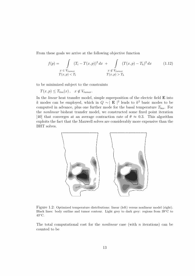
Figure 1.2: Optimized temperature distributions: linear (left) versus nonlinear model (right).Black lines: body outline and tumor contour. Light grey to dark grey: regions from 39◦C to43◦C.

The total computational cost for the nonlinear case (with n iterations) can becounted to be

13

costtotal = k ∗ costMaxwell +

n ∗ (costnlBHT + (k2 + 1) ∗ costlBHT + costOpt) (1.13)

where the notation is certainly self–explaining. We observed n ≈ 6. The total costfor the linear case is obtained by inserting costnlBHT = 0 and n = 1 above.

Upon comparing linear versus nonlinear perfusion models, significant differencesshow up. As can be seen in Fig. 1.2, the nonlinear model predicts a tumor heating,which from the therapeutic point of view is slightly preferable. The nonlinearmodel also influences the choice of optimal parameters for the k channels.

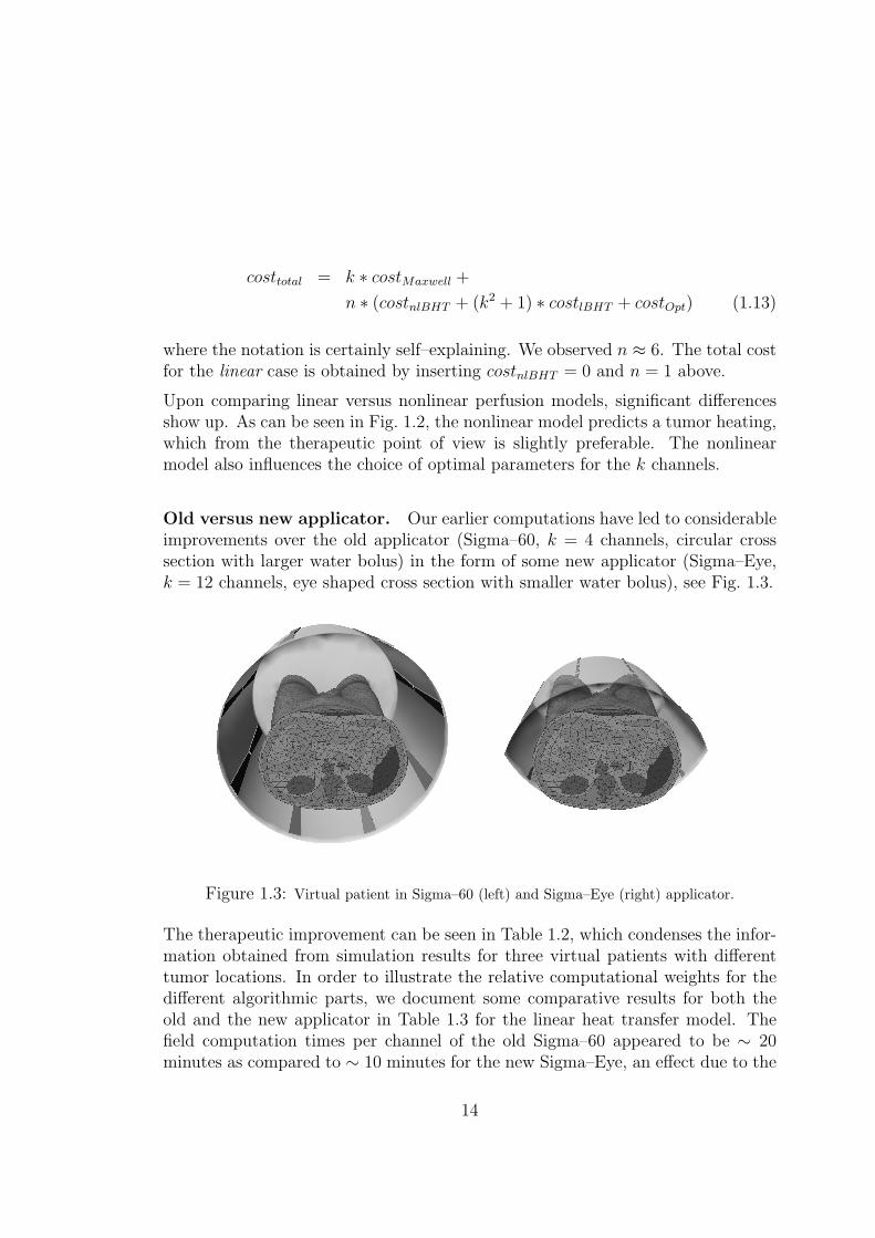
Old versus new applicator. Our earlier computations have led to considerableimprovements over the old applicator (Sigma–60, k = 4 channels, circular crosssection with larger water bolus) in the form of some new applicator (Sigma–Eye,k = 12 channels, eye shaped cross section with smaller water bolus), see Fig. 1.3.

Figure 1.3: Virtual patient in Sigma–60 (left) and Sigma–Eye (right) applicator.

The therapeutic improvement can be seen in Table 1.2, which condenses the infor-mation obtained from simulation results for three virtual patients with differenttumor locations. In order to illustrate the relative computational weights for thedifferent algorithmic parts, we document some comparative results for both theold and the new applicator in Table 1.3 for the linear heat transfer model. Thefield computation times per channel of the old Sigma–60 appeared to be ∼ 20minutes as compared to ∼ 10 minutes for the new Sigma–Eye, an effect due to the

14

smaller bolus volume. As expected, the temperature computation times roughlyscale with k2.

part of tumor volumeVirtual patient heated to above 43◦C

Sigma–60 Sigma–Eye

distal (supraanal) rectal carcinoma 17.5% 62.5

highly presacral rectal carcinoma 0.7% 18.4

cervical carcinoma at pelvic wall 24.8% 49.1

Table 1.2: Therapeutic improvement of new (Sigma–Eye) over old (Sigma–60) hyperthermiaapplicator.

Virtual Lab. The whole integrated software environment HyperPlan now con-sists of about 300.000 lines of code, wherein only about 120.000 lines are numericalcode, the other parts are segmentation algorithms, grid generation methods, andvisualization tools. This virtual lab has been recently sold to industry and willbe worldwide distributed together with the applicator hardware – increasing theapplicator’s efficiency significantly.

Sigma–60 Sigma–Eye

k = 4 k = 12

Segmentation 2 – 4 hours∗

Grid Generation 15 min∗∗

Field Calculations 80 min∗∗ 120 min∗∗

Temperature Calculations 2 min∗∗ 20 min∗∗

Optimization 6 sec∗∗ 1 min∗∗

∗ interactive∗∗ CPU time (SUN UltraSparc)

Table 1.3: Computation times per patient.

15

2 Partial Differential Equations in Optical Chip

Design

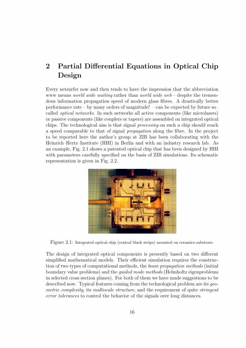
Every netsurfer now and then tends to have the impression that the abbreviationwww means world wide waiting rather than world wide web – despite the tremen-dous information propagation speed of modern glass fibres. A drastically betterperformance rate – by many orders of magnitude! – can be expected by future so–called optical networks. In such networks all active components (like microlasers)or passive components (like couplers or tapers) are assembled on integrated opticalchips. The technological aim is that signal processing on such a chip should reacha speed comparable to that of signal propagation along the fibre. In the projectto be reported here the author’s group at ZIB has been collaborating with theHeinrich–Hertz–Institute (HHI) in Berlin and with an industry research lab. Asan example, Fig. 2.1 shows a patented optical chip that has been designed by HHIwith parameters carefully specified on the basis of ZIB simulations. Its schematicrepresentation is given in Fig. 2.2.

Figure 2.1: Integrated optical chip (central black stripe) mounted on ceramics substrate.

The design of integrated optical components is presently based on two differentsimplified mathematical models. Their efficient simulation requires the construc-tion of two types of computational methods, the beam propagation methods (initialboundary value problems) and the guided mode methods (Helmholtz eigenproblemsin selected cross section planes). For both of them we have made suggestions to bedescribed now. Typical features coming from the technological problem are its geo-metric complexity, its multiscale structure, and the requirement of quite stringenterror tolerances to control the behavior of the signals over long distances.

16

Figure 2.2: Schematic representation of the chip in Fig. 2.1.

2.1 Beam Propagation Analysis

When modelling the signal propagation along a glass fibre, the fibre axis naturallyarises as a time–like coordinate z. In order to derive the so–called Fresnel

approximation, the electric field E is written in terms of a slowly varying amplitudeu as

E = ue−in0k0z , (2.1)

with k0 the vacuum wave number and n0 some effective refraction index to bespecified below. Assume that we start from Maxwell’s equations in the form (1.9).Let u depend on the propagation variable z and, for simplicity, only on one crosssection variable x. For ease of writing we redefine x := k0x, z := k0z, g := n2 −n2

0, c := 2in0. The specification of n0 comes in by some projection argument totake energy conservation in the Fresnel approximation at least to some extentinto account. This leads to

n20 =

(n2u, u) − (∇u,∇u)

(u, u). (2.2)

We thus end up with the normalized paraxial wave equation for the transversalelectrical mode (TE) in the form

Δu + g · u = cuz , (2.3)

which obviously is some complex Schrodinger–type equation. For pure beampropagation, we may even neglect the term uzz so that Δu here means just uxx.

17

This initial boundary value problem has been solved numerically in several techno-logical projects by F. Schmidt [76] using an adaptive Rothe method. As alreadydescribed in Section 1.1 above, this technique offers simultaneous adaptivity inboth time and space together with multilevel speed. However, the desirable adap-tivity cannot be fully exploited, unless suitable boundary conditions have beenconstructed, which are to be discussed next.

Discrete transparent boundary conditions. The idea behind the construc-tion of transparent boundary conditions (TB) for wave type equations is to re-strict the computations to some region of interest choosing boundary conditionssuch that waves touching the boundaries just pass these boundaries without anyreflections. For some time the canonical approach has been to start from a set ofTB derived from the continuous model, i.e. from the wave equation itself; these(non–local) boundary conditions were then discretized. However, proceeding likethat will often induce discretized reflected waves and even instability [68]. For thisreason, we derived a different approach in [78] that we called discrete transparentboundary conditions (DTB) – directly based on the Rothe method. Just like inthe continuous case, these DTB are also of nonlocal Cauchy type. In addition eachlinear implicit discretization scheme induces its own DTB.

In order to exemplify the approach, we return to the above PDE (2.3). In theRothe method the discretization for the time–like variable z, i.e. the direction ofpropagation, goes first. We deliberately apply the implicit midpoint rule, whichhas the selective feature that it conserves energy also in the discrete case. Conse-quently, any energy jumps observed in the course of the simulations must originatefrom the Fresnel approximation – a convenient and cheap monitor for the valid-ity of the employed model. After z–discretization of (2.3) neighboring time layers(i, i + 1) will be related according to (note: j =

√−1)

∂2ui+1

∂x2− λ2

i+1ui+1 = −∂2ui

∂x2+ κ2

i+1ui (2.4)

λ2i+1(x) :=

4jn0(zi + 12Δzi+1)

Δzi+1

− g(x, zi + 12Δzi+1)

κ2i+1(x) := −4jn0(zi + 1

2Δzi+1)

Δzi+1

− g(x, zi + 12Δzi+1)

σ2i+1(x) := 2g(x, zi + 1

2Δzi+1).

This relation defines a nested sequence of 1D boundary value problems for suc-cessive solutions ui(x) within some finite region of interest; let x = a denote one

18

of the boundaries. Note that we need not restrict the time steps Δzi to be con-stant. Following the lines of [78], the above non–local pattern can be taken intoaccount in terms of certain Laplace transforms Ui(p), which can be defined viathe recurrence relations

Ui+1(p) =ui+1(a) − ui(a)

p + λi+1

+ Ui(p) − σ2i+1

Ui(p) − Ui(λi+1)

p2 − λ2i+1

. (2.5)

Once this can be solved, the boundary values of the solution ui+1 at x = a aredefined by

∂(ui+1 − ui)

∂x

∣∣∣∣x=a

+ λi+1(ui+1(a) − ui(a)) = σ2i+1Ui(λi+1). (2.6)

Note that the new boundary conditions at time layer i+1 require the old boundaryconditions from time layer i and the term Ui(λi+1) so that the recurrence (2.5)should be evaluated at p = λi+2. Hence, whenever λi+1 = λi+2 – typically whenlocally constant stepsizes Δzi+1 = Δzi+2 and homogeneous materials occur – thenboth the denominator and the numerator in the third right hand term of (2.3)vanish: so some limit needs to be taken. Numerical trouble will already arise fornearly zeroes. For this reason, the above recurrence relation turned out to behard to stabilize numerically. Once this has been achieved (see [78]), the obtainedalgorithm was easy to realize. Summarizing, this type of DTB goes perfectlytogether with full adaptivity in space and time.

Remark. An even more elegant derivation of DTB by Schmidt and Yevick [79]applies some shift operator calculus. An inspired extension of DTB to the 2DHelmholtz equation can be found in the recent paper by Schmidt[77], who derivesand exploits some type of discrete Mikusinski operator calculus.

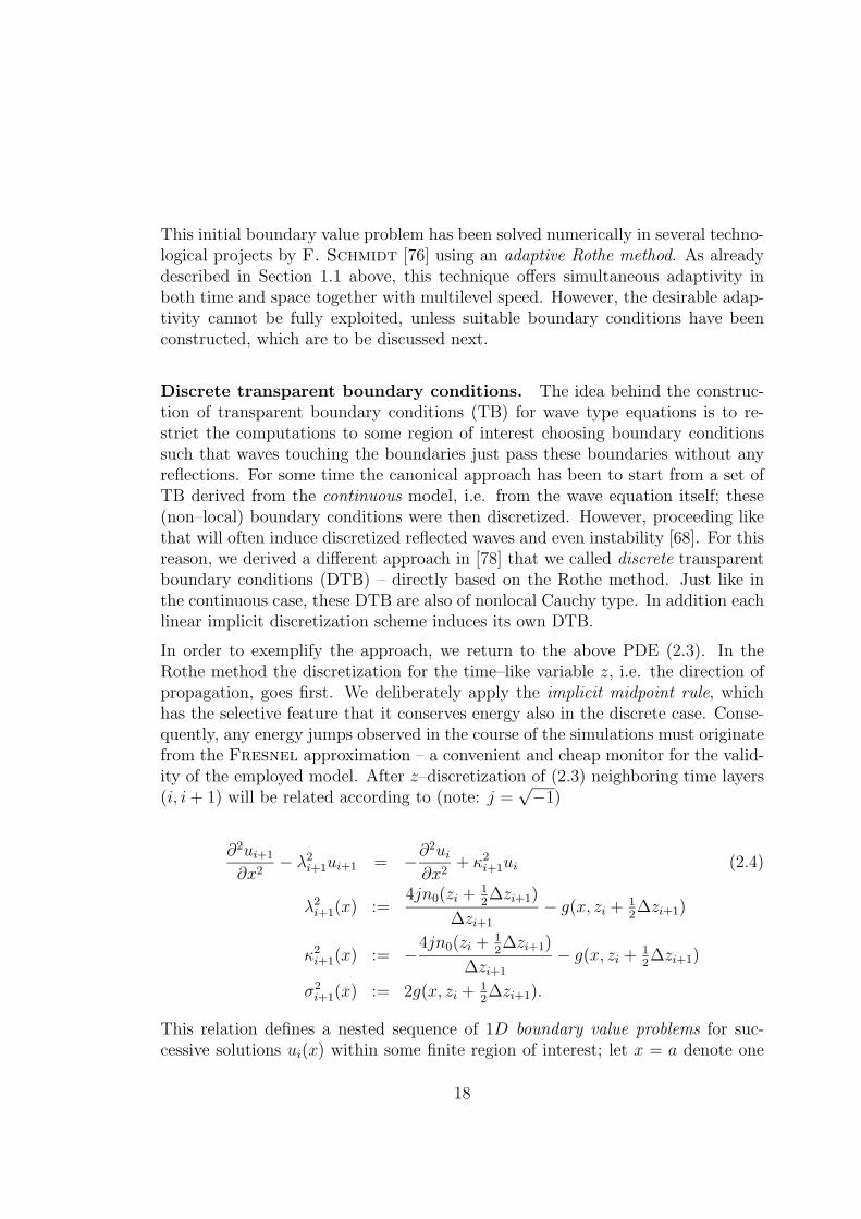
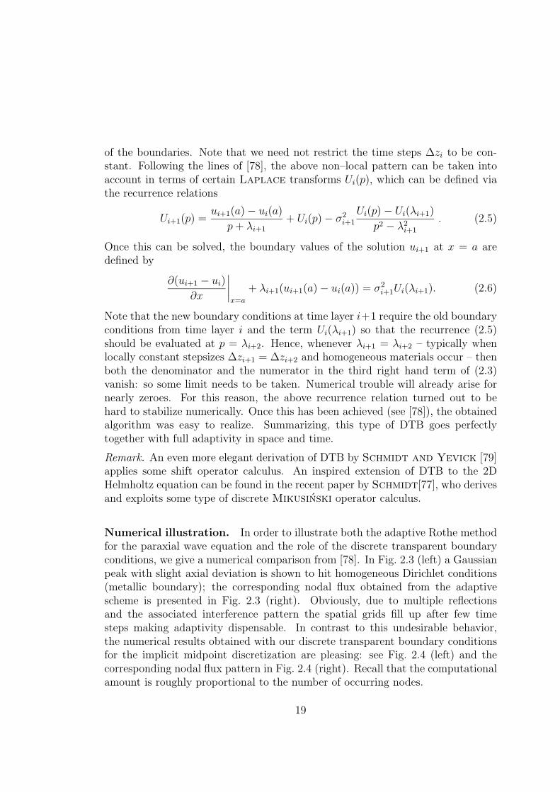
Numerical illustration. In order to illustrate both the adaptive Rothe methodfor the paraxial wave equation and the role of the discrete transparent boundaryconditions, we give a numerical comparison from [78]. In Fig. 2.3 (left) a Gaussianpeak with slight axial deviation is shown to hit homogeneous Dirichlet conditions(metallic boundary); the corresponding nodal flux obtained from the adaptivescheme is presented in Fig. 2.3 (right). Obviously, due to multiple reflectionsand the associated interference pattern the spatial grids fill up after few timesteps making adaptivity dispensable. In contrast to this undesirable behavior,the numerical results obtained with our discrete transparent boundary conditionsfor the implicit midpoint discretization are pleasing: see Fig. 2.4 (left) and thecorresponding nodal flux pattern in Fig. 2.4 (right). Recall that the computationalamount is roughly proportional to the number of occurring nodes.

19

0 2 4 6 8 10 12 14 16 18 20

20

40

60

80

100

120

140

160

180

200

220

+ + + + + + + + + + +

+

+

+

+

+

+

+

+

+

+

+

+ + + + + + + + ++++++++++++++++++++++++++++++++++++++++++++++++++++++++++++++++++++++ + + + + + + + ++ + + + + + + +++++++++++++++++++++++++++++++++++++++++++++++++++++++++++++++++++++++++++++++++++++++++++++++++++++++++++++++++++++++++ + + ++ + + + + ++++++++++++++++++++++++++++++++++++++++++++++++++++++++++++++++++++++++++++++++++++++++++++++++++++++++++++++++++++++++++++++++++++++++++++++++++ + + + + + + + ++ + + + + +++++++++++++++++++++++++++++++++++++++++++++++++++++++++++++++++++++++++++++++++++++++++++++++++++++++++++ + + + + ++ + + + + +++++++++++++++++++++++++++++++++++++++++++++++++++++++++++++++++++++++++++++++++++++++++++++++++++ + + ++ + + + + ++++++++++++++++++++++++++++++++++++++++++++++++++++++++++++++++++++++++++++++++++++++++++++++++++++++++++++++++++++++++ + + + + ++ + + + + + ++++++++++++++++++++++++++++++++++++++++++++++++++++++++++++++++++++++++++++++++++++++++++++++++++++++++++++++++++++++++++++++++++++++++++++++++++ + + + + ++ + + ++++++++++++++++++++++++++++++++++++++++++++++++++++++++++++++++++++++++++++++++++++++++++++++++++++++++++++++++++++++++++++++++++++++++++++++ + + + + + + ++ + + + + +++++++++++++++++++++++++++++++++++++++++++++++++++++++++++++++++++++++++++++++++++++++++++++++++++++++++++++++++++++++++++++++++++++++++++++++++ + + + + + + ++ + + + + +++++++++++++++++++++++++++++++++++++++++++++++++++++++++++++++++++++++++++++++++++++++++++++++++++++++++++++++++++++++++++++++++++++++++++++++++++++++++++ + + + + + + ++ + + + + +++++++++++++++++++++++++++++++++++++++++++++++++++++++++++++++++++++++++++++++++++++++++++++++++++++++++++++++++++++++++++++++++++++++++++++++++++++++++++++++++++++++++++++++++++++++++++++++++++++ + + + + + + ++ + + + ++++++++++++++++++++++++++++++++++++++++++++++++++++++++++++++++++++++++++++++++++++++++++++++++++++++++++++++++++++++++++++++++++++++++++++++++ +++ + + + + + + ++ + + + ++++++++++++++++++++++++++++++++++++++++++++++++++++++++++++++++++++++++++++++++++++++++++++++++++++++++++++++++++++++++++++++++++++++++++++++++++++++++++++++++++++++ +++ +++ + + + + + ++ + + +++++++++++++++++++++++++++++++++++++++++++++++++++++++++++++++++++++++++++++++++++++++++++++++++++++++++++++++++++++++++++++++++++++++++++++++++++++++++++++++++++++++++++++++++++++++++++++++++++++++++++++++++++++++++++++++++++ + + + + + + + ++ +++++++++++++++++++++++++++++++++++++++++++++++++++++++++++++++++++++++++++++++++++++++++++++++++++++++++++++++++++++++++++++++++++++++++++++++++++++++++++++++++++++++++++++++++++++++++++++++++++++++++++++++++++++++++++++++++++++++++ + +++ + + + + + + +++++++++++++++++++++++++++++++++++++++++++++++++++++++++++++++++++++++++++++++++++++++++++++++++++++++++++++++++++++++++++++++++++++++++++++++++++++++++++++++++++++++++++++++++++++++++++++++++++++++++++++++++++++ + + + + + + ++++++++++++++++++++++++++++++++++++++++++++++++++++++++++++++++++++++++++++++++++++++++++++++++++++++++++++++++++++++++++++++++++++++++++++++++++++++++++++++++++++++++++++++++++++++++++++++++++++++++++++++++++++++++++++++++++++++++++++++++++++++++ +++++ + + + + + + + + ++++++++++++++++++++++++++++++++++++++++++++++++++++++++++++++++++++++++++++++++++++++++++++++++++++++++++++++++++++++++++++++++++++++++++++++++++++++++++++++++++++++++++++++++++++++++++++++++++++++++++++++++++++++++++++++++++++++++ +++++++++++ +++++ + + + +++++++++++++++++++++++++++++++++++++++++++++++++++++++++++++++++++++++++++++++++++++++++++++++++++++++++++++++++++++++++++++++++++++++++++++++++++++++++++++++++++++++++++++++++++++++++++++++++++++++++ +++++ +++++ + + + + + + + ++++++++++++++++++++++++++++++++++++++++++++++++++++++++++++++++++++++++++++++++++++++++++++++++++++++++++++++++++++++++++++++++++++++++++++++++++++++++++++++++++++++++++++++++++++++++++++++++++++++++++++++++++++++++++++++++++++++++++++++++++++ + +++++ + + + + + + +++++++++++++++++++++++++++++++++++++++++++++++++++++++++++++++++++++++++++++++++++++++++++++++++++++++++++++++++++++++++++++++++++++++++++++++++++++++++++++++++++++++++++++++++++++++++++++++++++++ + + + + + + + + + + + ++++++++++++++++++++++++++++++++++++++++++++++++++++++++++++++++++++++++++++++++++++++++++++++++++++++++++++++++++++++++++++++++++++++++++++++++++++++++++++++++++++++++++++++++++++++++++++++++++++++++++++ + + + + + + + + + + +++++++++++++++++++++++++++++++++++++++++++++++++++++++++++++++++++++++++++++++++++++++++++++++++++++++++++++++++++++++++++++++++++++++++++++++++++++++++++++++++++++++++++++++++++++++++++++++++++++++++++++++++++++++++++++++++++++++ + + + + + + + + + + + + ++++++++++++++++++++++++++++++++++++++++++++++++++++++++++++++++++++++++++++++++++++++++++++++++++++++++++++++++++++++++++++++++++++++++++++++++++++++++++++++++++++++++++++++++++++++++++++++++++++++++++++++++++++++++++++++++++++++++++++ + + + + + + + + ++++++++++++++++++++++++++++++++++++++++++++++++++++++++++++++++++++++++++++++++++++++++++++++++++++++++++++++++++++++++++++++++++++++++++++++++++++++++++++++++++++++++++++++++++++++++++++++++++++++++++++++++++++++ + + + + + + + ++++++++++++++++++++++++++++++++++++++++++++++++++++++++++++++++++++++++++++++++++++++++++++++++++++++++++++++++++++++++++++++++++++++++++++++++++++++++++++++++++++++++++++ + + + + + + + + + + +++++++++++++++++++++++++++++++++++++++++++++++++++++++++++++++++++++++++++++++++++++++++++++++++++++++++++++++++++++++++++++++++++++++++++ + + + + + + + + + + + + + ++++++++++++++++++++++++++++++++++++++++++++++++++++++++++++++++++++++++++++++++++++++++++++++++++++++++++++++++++++++++++++++++++++++++++++++++++++ + + + + + + + + + + + + + + + +++++++++++++++++++++++++++++++++++++++++++++++++++++++++++++++++++++++++++++++++++++++++++++++++++++++++++++++++++++++++++++++++++++++++++++++++++++++++++++++++++++ + +++ + + + + + + + + + + + + + +++++++++++++++++++++++++++++++++++++++++++++++++++++++++++++++++++++++++++++++++++++++++++++++++++++++++++++++++++++++++++++++++++++++++++++++++++++++++++++++++++++++++++++++++++++++ +++++++++ +++++ + + +++ + + + + + + + + +++++++++++++++++++++++++++++++++++++++++++++++++++++++++++++++++++++++++++++++++++++++++++++++++++++++++++++++++++++++++++++++++++++++++++++++++++++++++++++++++++++++++++++++++++++++++++++++++++++++++++++++++++ +++++ + + + + + + + + + +++++++++++++++++++++++++++++++++++++++++++++++++++++++++++++++++++++++++++++++++++++++++++++++++++++++++++++++++++++++++++++++++++++++++++++++++++++++++++++++++++ +++++ + + + + + + + + + + +++++++++++++++++++++++++++++++++++++++++++++++++++++++++++++++++++++++++++++++++++++++++++++++++++++++++++++++++++++++++++++++++++++++++++++++++++++++++++++++++++++++++++++++++++++++++++++++++++++ + + + + + + + ++++++++++++++++++++++++++++++++++++++++++++++++++++++++++++++++++++++++++++++++++++++++++++++++++++++++++++++++++++++++++++++++++++++++++++++++++++++++++++++++++++++++++++++++++++++++++++++++++++++++ + + + + + + + +++++++++++++++++++++++++++++++++++++++++++++++++++++++++++++++++++++++++++++++++++++++++++++++++++++++++++++++++++++++++++++++++++++++++++++++++++++++++++++++++++++++++++++++++++++++++++++++++++++++++++++++++++++++++++++++++++++++++++++++++++++++++++++++ + + + + + + ++++++++++++++++++++++++++++++++++++++++++++++++++++++++++++++++++++++++++++++++++++++++++++++++++++++++++++++++++++++++++++++++++++++++++++++++++++++++++++++++++++++++++++++++++++++++++++++++++++++++++++++++++++++++++++++++++++++++++++++++++++++++++++++++++ + + + + ++++++++++++++++++++++++++++++++++++++++++++++++++++++++++++++++++++++++++++++++++++++++++++++++++++++++++++++++++++++++++++++++++++++++++++++++++++++++++++++++++++++++++++++++++++++++++++++++++++++++++++++++++++++++ + + + + +++++++++++++++++++++++++++++++++++++++++++++++++++++++++++++++++++++++++++++++++++++++++++++++++++++++++++++++++++++++++++++++++++++++++++++++++++++++++++++++++++++++++++++++++++++++++++++++++++++++++++++++++++++++++++++++++++++++++++++++++++++++++++++++++++++++++ + + + + +++++++++++++++++++++++++++++++++++++++++++++++++++++++++++++++++++++++++++++++++++++++++++++++++++++++++++++++++++++++++++++++++++++++++++++++++++++++++++++++++++++++++++++++++++++++++++++++++++++++++++++++++++++++++++++++++++++++++++++++++++++ + + + + + + +++++++++++++++++++++++++++++++++++++++++++++++++++++++++++++++++++++++++++++++++++++++++++++++++++++++++++++++++++++++++++++++++++++++++++++++++++++++++++++++++++++++++++++++++++++++++++++++++++++++++++++++++++++++++++++++++++++++++++++++++++++++++++++++++++++++ + + + +++++++++++++++++++++++++++++++++++++++++++++++++++++++++++++++++++++++++++++++++++++++++++++++++++++++++++++++++++++++++++++++++++++++++++++++++++++++++++++++++++++++++++++++++++++++++++++++++++++++++++++++++++++++++++++++++++++++++++++++++++++++++++++++++++++++++++++++++++++++++++++++++++++++++++++++++++++++++++++++ + + +++++++++++++++++++++++++++++++++++++++++++++++++++++++++++++++++++++++++++++++++++++++++++++++++++++++++++++++++++++++++++++++++++++++++++++++++++++++++++++++++++++++++++++++++++++++++++++++++++++++++++++++++++++++++++++++++++++++++++++++++++++++++++++++++++++++++++++++++++++++++++++++++++++++++++++++++++++++++++++++++++ + + + +++++++++++++++++++++++++++++++++++++++++++++++++++++++++++++++++++++++++++++++++++++++++++++++++++++++++++++++++++++++++++++++++++++++++++++++++++++++++++++++++++++++++++++++++++++++++++++++++++++++++++++++++++++++++++++++++++++++++++++++++++++++++++++++++++++++++++++++++++++++++++++++++++++++++++++++++++++++++++++++++++++++ + + + + + +++++++++++++++++++++++++++++++++++++++++++++++++++++++++++++++++++++++++++++++++++++++++++++++++++++++++++++++++++++++++++++++++++++++++++++++++++++++++++++++++++++++++++++++++++++++++++++++++++++++++++++++++++++++++++++++++++++++++++++++++++++++++++++++++++++++++++++++++++++++++++++++++++++++++++++++++++++++++++++++++++++++++++++++++++++++++++++++++++++++++++++++++++++++++++++++++++ + +++++++++++++++++++++++++++++++++++++++++++++++++++++++++++++++++++++++++++++++++++++++++++++++++++++++++++++++++++++++++++++++++++++++++++++++++++++++++++++++++++++++++++++++++++++++++++++++++++++++++++++++++++++++++++++++++++++++++++++++++++++++++++++++++++++++++++++++++++++++++++++++++++++++++++++++++++++++++++++++++++++++++++++++++++++++++++++++++++++++++++++++++++++++++++++++++++++++++++++++++++++++++++++++++++++++++++++++++++++++++++++++++++++++++++++++++++++++++++++++++++++++++++++++++++++++++++++++++++++++++++++++++++++++++++++++++++++++++++++++++++++++++++++++++++++++++++++++++++++++++++++++++++++++++++++++++++++++++++++++++++++++++++++++++++++++++++++++++++++++++++++++++++++++++++++++++++++++++++++++++++++++++++++++++++++++++++++++++++++++++++++++++++++++++++++++++++++++++++++++++++++++++++++++++++++++++++++++++++++++++++++++++++++++++++++++++++++++++++++++++++++++++++++++++++++++++++++++++++++++++++++++++++++++++++++++++++++++++++++++++++++++++++++++++++++++++++++++++++++++++++++++++++++++++++++++++++++++++++++++++++++++++++++++++++++++++++++++++++++++++++++++++++++++++++++++++++++++++++++++++++++++++++++++++++++++++++++++++++++++++++++++++++++++++++++++++++++++++++++++++++++++++++++++++++++++++++++++++++++++++++++++++++++++++++++++++++++++++++++++++++++++++++++++++++++++++++++++++++++++++++++++++++++++++++++++++++++++++++++++++++++++++++++++++++++++++++++++++++++++++++++++++++++++++++++++++++++++++++++++++++++++++++++++++++++++++++++++++++++++++++++++++++++++++++++++++++++++++++++++++++++++++++++++++++++++++++++++++++++++++++++++++++++++++++++++++++++++++++++++++++++++++++++++++++++++++++++++++++++++++++++++++++++++++++++++++++++++++++++++++++++++++++++++++++++++++++++++++++++++++++++++++++++++++++++++++++++++++++++++++++++++++++++++++++++++++++++++++++++++++++++++++++++++++++++++++++++++++++++++++++++++++++++++++++++++++++++++++++++++++++++++++++++++++++++++++++++++++++++++++++++++++++++++++++++++++++++++++++++++++++++++++++++++++++++++++++++++++++++++++++++++++++++++++++++++++++++++++++++++++++++++++++++++++++++++++++++++++++++++++++++++++++++++++++++++++++++++++++++++++++++++++++++++++++++++++++++++++++++++++++++++++++++++++++++++++++++++++++++++++++++++++++++++++++++++++++++++++++++++++++++++++++++++++++++++++++++++++++++++++++++++++++++++++++++++++++++++++++++++++++++++++++++++++++++++++++++++++++++++++++++++++++++++++++++++++++++++++++++++++++++++++++++++++++++++++++++++++++++++++++++++++++++++++++++++++++++++++++++++++++++++++++++++++++++++++++++++++++++++++++++++++++++++++++++++++++++++++++++++++++++++++++++++++++++++++++++++++++++++++++++++++++++++++++++++++++++++++++++++++++++++++++++++++++++++++++++++++++++++++++++++++++++++++++++++++++++++++++++++++++++++++++++++++++++++++++++++++++++++++++++++++++++++++++++++++++++++++++++++++++++++++++++++++++++++++++++++++++++++++++++++++++++++++++++++++++++++++++++++++++++++++++++++++++++++++++++++++++++++++++++++++++++++++++++++++++++++++++++++++++++++++++++++++++++++++++++++++++++++++++++++++++++++++++++++++++++++++++++++++++++++++++++++++++++++++++++++++++++++++++++++++++++++++++++++++++++++++++++++++++++++++++++++++++++++++++++++++++++++++++++++++++++++++++++++++++++++++++++++++++++++++++++++++++++++++++++++++++++++++++++++++++++++++++++++++++++++++++++++++++++++++++++++++++++++++++++++++++++++++++++++++++++++++++++++++++++++++++++++++++++++++++++++++++++++++++++++++++++++++++++++++++++++++++++++++++++++++++++++++++++++++++++++++++++++++++++++++++++++++++++++++++++++++++++++++++++++++++++++++++++++++++++++++++++++++++++++++++++++++++++++++++++++++++++++++++++++++++++++++++++++++++++++++++++++++++++++++++++++++++++++++++++++++++++++++++++++++++++++++++++++++++++++++++++++++++++++++++++++++++++++++++++++++++++++++++++++++++++++++++++++++++++++++++++++++++++++++++++++++++++++++++++++++++++++++++++++++++++++++++++++++++++++++++++++++++++++++++++++++++++++++++++++++++++++++++++++++++++++++++++++++++++++++++++++++++++++++++++++++++++++++++++++++++++++++++++++++++++++++++++++++++++++++++++++++++++++++++++++++++++++++++++++++++++++++++++++++++++++++++++++++++++++++++++++++++++++++++++++++++++++++++++++++++++++++++++++++++++++++++++++++++++++++++++++++++++++++++++++++++++++++++++++++++++++++++++++++++++++++++++++++++++++++++++++++++++++++++++++++++++++++++++++++++++++++++++++++++++++++++++++++++++++++++++++++++++++++++++++++++++++++++++++++++++++++++++++++++++++++++++++++++++++++++++++++++++++++++++++++++++++++++++++++++++++++++++++++++++++++++++++++++++++++++++++++++++++++++++++++++++++++++++++++++++++++++++++++++++++++++++++++++++++++++++++++++++++++++++++++++++++++++++++++++++++++++++++++++++++++++++++++++++++++++++++++++++++++++++++++++++++++++++++++++++++++++++++++++++++++++++++++++++++++++++++++++++++++++++++++++++++++++++++++++++++++++++++++++++++++++++++++++++++++++++++++++++++++++++++++++++++++++++++++++++++++++++++++++++++++++++++++++++++++++++++++++++++++++++++++++++++++++++++++++++++++++++++++++++++++++++++++++++++++++++++++++++++++++++++++++++++++++++++++++++++++++++++++++++++++++++++++++++++++++++++++++++++++++++++++++++++++++++++++++++++++++++++++++++++++++++++++++++++++++++++++++++++++++++++++++++++++++++++++++++++++++++++++++++++++++++++++++++++++++++++++++++++++++++++++++++++++++++++++++++++++++++++++++++++++++++++++++++++++++++++++++++++++++++++++++++++++++++++++++++++++++++++++++++++++++++++++++++++++++++++++++++++++++++++++++++++++++++++++++++++++++++++++++++++++++++++++++++++++++++++++++++++++++++++++++++++++++++++++++++++++++++++++++++++++++++++++++++++++++++++++++++++++++++++++++++++++++++++++++++++++++++++++++++++++++++++++++++++++++++++++++++++++++++++++++++++++++++++++++++++++++++++++++++++++++++++++++++++++++++++++++++++++++++++++++++++++++++++++++++++++++++++++++++++++++++++++++++++++++++++++++++++++++++++++++++++++++++++++++++++++++++++++++++++++++++++++++++++++++++++++++++++++++++++++++++++++++++++++++++++++++++++++++++++++++++++++++++++++++++++++++++++++++++++++++++++++++++++++++++++++++++++++++++++++++++++++++++++++++++++++++++++++++++++++++++++++++++++++++++++++++++++++++++++++++++++++++++++++++++++++++++++++++++++++++++++++++++++++++++++++++++++++++++++++++++++++++++++++++++++++++++++++++++++++++++++++++++++++++++++++++++++++++++++++++++++++++++++++++++++++++++++++++++++++++++++++++++++++++++++ ++++++++++++++++++++++++++++++++++++++++++++++++++++++++++++++++++++++++++++++++++++++++++++++++++++++++++++++++++++++++++++++++++++++++++++++++++++++++++++++++++++++++++++++++++++++++++++++++++++++++++++++++++++++++++++++++++++++++++++++++++++++++++++++++++++++++++++++++++++++++++++++++++++++++++++++++++++++++++++++++++++++++++++++++++++++++++++++++++++++++++++++++++++++++++++++++++++++++++++++++++++++++++++++++++++++++++++++++++++++++++++++++++++++++++++++++++++++++++++++++++++++++++++++++++++++++++++++++++++++++++++++++++++++++++++++++++++++++++++++++++++++++++++++++++++++++++++++++++++++++++++++++++++++++++++++++++++++++++++++++++++++++++++++++++++++++++++++++++++++++++++++++++++++++++++++++++++++++++++++++++++++++++++++++++++++++++++++++++++++++++++++++++++++++++++++++++++++++++++++++++++++++++++++++++++++++++++++++++++++++++++++++++++++++++++++++++++++++++++++++++++++++++++++++++++++++++++++++++++++++++++++++++++++++++++++++++++++++++++++++++++++++++++++++++++++++++++++++++++++++++++++++++++++++++++++++++++++++++++++++++++++++++++++++++++++++++++++++++++++++++++++++++++++++++++++++++++++++++++++++++++++++++++++++++++++++++++++++++++++++++++++++++++++++++++++++++++++++++++++++++++++++++++++++++++++++++++++++++++++++++++++++++++++++++++++++++++++++++++++++++++++++++++++++++++++++++++++++++++++++++++++++++++++++++++++++++++++++++++++++++++++++++++++++++++++++++++++++++++++++++++++++++++++++++++++++++++++++++++++++++++++++++++++++++++++++++++++++++++++++++++++++++++++++++++++++++++++++++++++++++++++++++++++++++++++++++++++++++++++++++++++++++++++++++++++++++++++++++++++++++++++++++++++++++++++++++++++++++++++++++++++++++++++++++++++++++++++++++++++++++++++++++++++++++++++++++++++++++++++++++++++++++++++++++++++++++++++++++++++++++++++++++++++++++++++++++++++++++++++++++++++++++++++++++++++++++++++++++++++++++++++ +++++++++++++++++++++++++++++++++++++++++++++++++++++++++++++++++++++++++++++++++++++++++++++++++++++++++++++++++++++++++++++++++++++++++++++++++++++++++++++++++++++++++++++++++++++++++++++++++++++++++++++++++++++++++++++++++++++++++++++++++++++++++++++++++++++++++++++++++++++++++++++++++++++++++++++++++++++++++++++++++++++++++++++++++++++++++++++++++++++++++++++++++++++++++++++++++++++++++++++++++++++++++++++++++++++++++++++++++++++++++++++++++++++++++++++++++++++++++++++++++++++++++++++++++++++++++++++++++++++++++++++++++++++++++++++++++++++++++++++++++++++++++++++++++++++++++++++++++++++++++++++++++++++++++++++++++++++++++++++++++++++++++++++++++++++++++++++++++++++++++++++++++++++++++++++++++++++++++++++++++++++++++++++++++++++++++++++++++++++++++++++++++++++++++++++++++++++++++++++++++++++++++++++++++++++++++++++++++++++++++++++++++++++++++++++++++++++++++++++++++++++++++++++++++++++++++++++++++++++++++++++++++++++++++++++++++++++++++++++++++++++++++++++++++++++++++++++++++++++++++++++++++++++++++++++++++++++++++++++++++++++++++++++++++++++++++++++++++++++++++++++++++ +++++++++++++++++++++++++ +++++++++++++++++++++++++++++++++++++++++++++++++++++++++++++++++++++++++++++++++++++++++++++++++++++++++++++++++++++++++++++++++++++++++++++++++++++++++++++++++++++++++++++++++++++++++++++++++++++++++++++++++++++++++++++++++++++++++++++++++++++++++++++++ +++++++++++++++++++++++++++++++++++++++++++++++++ +++++++++++++ + +++++++++++++++++++++++++++++++++++++++++++++++++++++++++++++++++++++++++++++++++++++++++++++++++++++++++++++++++++++++++++++++++++++++++++++++++++++++++++++++++++++++++++++++++++++++++++++++++++++++++++++++++++++++++++++++++++++++++++++++++++++++++++++++++++++++++++++++++++++ ++++++++++++++++++++++++++++++++++++++++++++++++++++++++++++++++++++++++++++++++++++++++++++++++++++++++++++++++++++++++++++++++++++++++++++++++++++++++++++++++++++++++++++++++++++++++++++++++++++++++++++++++++++++++++++++++++++++++++++++++++++++++++++++++++++++++++++++++++++ +++++++++++++++++++++++++++++++++++++++++++++++++++++++++++++++++++++++++++++++++++++++++++++++++++++++++++++++++++++++++++ +++++++++++++++++++++++ +++++++++++++++++++++++++++++++++++++++++++++++++++++++++++++++++++++++++++++++++++++++++++++++++++++++++++++++++++++++++++++++++++++++++++++++++++++++++++++++++++++++++++++++++++++++++++++++++++++++++++++++++++++++++++++++++++++++++++++++++++++++++++++++ ++++++++++++++++++++++++++++++++++++++++++++++++++++++++++++++++++++++++++++++++++++++++++++++++++++++++++++++++++++++++++++++++++++++++++++++++++++++++++++++++++++++++++++++++++++++++++++++++++++++++++++++++++++++++++++++++++++++++++++++++++++++++++++++++++++++++++++++++++++++++++++++++++++++++++++++++++++++++++++++++++++++++++++++++++++++++++++++++++++++++++++++++++++++++++++++++++++++++++++++++++++++++++++++++++++++++ +++++++++++++++++++++++++++++++++++++++++++++++++++++++++++++++++++++++++++++++++++++++++++++++++++++++++++++++++++++++++++++++++++++++++++++++++++++++++++++++++++++++++++++++++++++++++++++++++++++++++++++++++++++++++++++++++++++++++++++++++++++++++++++++++++++++++++++++++++++++++++++++++++++++++++++++++++++++++++++ ++++++++++++++ + ++++++++++++++++++++++++++++++++++++++++++++++++++++++++++++++++++++++++++++++++++++++++++++++++++++++++++++++++++++++++++++++++++++++++++++++++++++++++++++++++++++++++++++++++++++++++++++++++++++++++++++++++++++++++++++++++++++++++++++++++++++++++++++++++++++++++++++++++++++++++++++++++++++++++++++++++++++++++++++++++++++++++++++++++++++++++++++++++++++++++++++++++++++++++++++++++++++++++++++++++++++++++++++++++++++++++++++++++++++++++++++++++++++++++++++++++++++++++++++++++++++++++++++++++++++++++++++++++++++++++++++++++++++++++++++++++++++++++++++++++++++++++++++++++++++++++++++++++++++++++++++++++++++++++++++++++++++++++++++++++++++++++++++++++++++++++++++++++++++++++++++++++++++++++++++++++++++++++++++++++++++++++++++++++++++++++++++++++++++++++++++++++++++++++++++++++++++++++++++++++++++++++++++++++++++++++++++++++++++++++++++++++++++++++++++++++++++++++++++++++++++++++++++++++++++++++++++++++++++++++++++++++++++++++++++++++++++++++++++++++++++++++++++++++++++++++++++++++++++++++++++++++++++++++++++++++++++++++++++++++++++++++++++++++++++++++++++++++++++++++++++++++++++++++++++++++++++++++++++++++++++++++++++++++++++++++++++++++++++++++++++++++++++++++++++++++++++++++++++++++++++++++++++++++++++++++++++++++++++++++++++++++++++++++++++++++++++++++++++++++++++++++++++++++++++++++++++++++++++++++++++++++++++++++++++++++++++++++++++++++++++++++++++++++++++++++++++++++++++++++++++++++++++++++++++++++++++++++++++++++++++++++++++++++++++++++++++++++++++++++++++++++++++++++++++++++++++++++++++++++++++++++++++++++++++++++++++++++++++++++++++++++++++++++++++++++++++++++++++++++++++++++++++++++++++++++++++++++++++++++++++++++++++++++++++++++++++++++++++++++++++++++++++++++++++++++++++++++++++++++++++++++++++++++++++++++++++++++++++++++++++++++++++++++++++++++++++++++++++++++++++++++++++++++++++++++++++++++++++++++++++++++++++++++++++++++++++++++++++++++++++++++++++++++++++++++++++++++++++++++++++++++++++++++++++++++++++++++++++++++++++++++++++++++++++++++++++++++++++++++++++++++++++++++++++++++++++++++++++++++++++++++++++++++++++++++++++++++++++++++++++++++++++++++++++++++++++++++++++++++++ ++++++++++++++++++++++++++++++++++++++++++++++++++++++++++++++++++++++++++++++++++++++++++++++++++++++++++++++++++++++++++++++++++++++++++++++++++++++++++++++++++++++++++++++++++++++++++++++++++++++++++++++++++++++++++++++++++++++++++++++++++++++++++++++++++++++++++++++++++++++++++++++++++++++++++++++++++++++++++++++++++++++++++++++++++++++++++++++++++++++++++++++++++++++++++++++++++++++++++++++++++++++++++++++++++++++++++++++++++++++++++++++++++++++++++++++++++++++++++++++++++++++++++++++++++++++++++++++++++++++++++++++++++++++++++++++++++++++++++++++++++++++++++++++++++++++++++++++++++++++++++++++++++++++++++++++++++++++++++++++++++++++++++++++++++++++++++++++++++++++++++++++++++++++++++++++++++++++++++++++++++++++++++++++++++++++++++++++++++++++++++++++++++++++++++++++++++++++++++++++++++++++++++++++++++++++++++++++++++++++++++++++++++++++++++++++++++++++++++++++++++++++++++++++++++++++++++++++++++++++++++++++++++++++++++++++++++++++++++++++++++++++++++++++++++++++++++++++++++++++++++++++++++++++++++++++++++++++++++++++++++++++++++++++++++++++++++++++++++++++++++++++++++++++++++++++++++++++++++++++++++++++++++++++++++++++++++++++++++++++++++++++++++++++++++++++++++++++++++++++++++++++++++++++++++++++++++++++++++++++++++++++++++++++++++++++++++++++++++++++++++++++++++++++++++++++++++++++++++++++++++++++++++++++++++++++++++++++++++++++++++++++++++++++++++++++++++++++++++++++++++++++++++++++++++++++++++++++++++++++++++++++++++++++++++++++++++++++++++++++++++++++++++++++++++++++++++++++++++++++++++++++++++++++++++++++++++++++++++++++++++++++++++++++++++++++++++++++++++++++++++++++++++++++++++++++++++++++++++++++++++++++++++++++++++++++++++++++++++++++++++++++++++++++++++++++++++++++++++++++++++++++++++++++++++++++++++++++++++++++++++++++++++++++++++++++++++++++++++++++++++++++++++++++++++++++++++++++++++++++++++++++++++++++++++++++++++++++++++++++++++++++++++++++++++++++++++++++++++++++++++++++++++++++++++++++++++++++++++++++++++++++++++++++++++++++++++++++++++++++++++++++++++++++++++++++++++++++++++++++++++++++++++++++++++++++++++++++++++++++++++++++++++++++++++++++++++++++++++++++++++++++++++++++++++++++++++++++++++++++++++++++++++++++++++++++++++++++++++++++++++++++++++++++++++++++++++++++++++++++++++++++++++++++++++++++++++++++++++++++++++++++++++++++++++++++++++++++++++++++++++++++++++++++++++++++++++++++++++++++++++++++++++++++++++++++++++++++++++++++++++++++++++++++++++++++++++++++++++++++++++++++++++++++++++++++++++++++++++++++++++++++++++++++++++++++++++++++++++++++++++++++++++++++++++++++++++++++++++++++++++++++++++++++++++++++++++++++++++++++++++++++++++++++++++++++++++++++++++++++++++++++++++++++++++++++++++++++++++++++++++++++++++++++++++++++++++++++++++++++++++++++++++++++++++++++++++++++++++++++++++++++++++++++++++++++++++++++++++++++++++++++++++++++++++++++++++++++++++++++++++++++++++++++++++++++++++++++++++++++++++++++++++++++++++++++++++++++++++++++++++++++++++++++++++++++++++++++++++++++++++++++++++++++++++++++++++++++++++++++++++++++++++++++++++++++++++++++++++++++++++++++++++++++++++++++++++++++++++++++++++++++++++++++++++++++++++++++++++++++++++++++++++++++++++++++++++++++++++++++++++++++++++++++++++++++++++++++++++++++++++++++++++++++++++++++++++++++++++++++++++++++++++++++++++++++++++++++++++++++++++++++++++++++++++++++++++++++++++++++++++++++++++++++++++++++++++++++++++++++++++++++++++++++++++++++++++++++++++++++++++++++++++++++++++++++++++++++++++++++++++++++++++++++++++++++++++++++++++++++++++++++++++++++++++++++++++++++++++++++++++++++++++++++++++++++++++++++++++++++++++++++++++++++++++++++++++++++++++++++++++++++++++++++++++++++++++++++++++++++++++++++++++++++++++++++++++++++++++++++++++++++++++++++++++++++++++++++++++++++++++++++++++++++++++++++++++++++++++++++++++++++++++++++++++++++++++++++++++++++++++++++++++++++++++++++++++++++++++++++++++++++++++++++++++++++++++++++++++++++++++++++++++++++++++++++++++++++++++++++++++++++++++++++++++++++++++++++++++++++++++++++++++++++++++++++++++++++++++++++++++++++++++++++++++++++++++++++++++++++++++++++++++++++++++++++++++++++++++++++++++++++++++++++++++++++++++++++++++++++++++++++++++++++++++++++++++++++++++++++++++++++++++++++++++++++++++++++++++++++++++++++++++++++++++++++++++++++++++++++++++++++++++++++++++++++++++++++++++++++++++++++++++++++++++++++++++++++++++++++++++++++++++++++++++++++++++++++++++++++++++++++++++++++++++++++++++++++++++++++++

0 2 4 6 8 10 12 14 16 18 20

20

40

60

80

100

120

140

160

180

200

+ + + + + + + + + + +

+

+

+

+

+

+

+

+

+

+

z/μm

x/μm

z/μm

x/μm

Figure 2.3: Gaussian peak propagation with metallic boundary conditions. Left: solution withinterference pattern. Right: corresponding nodal flux.

0 2 4 6 8 10 12 14 16 18 20

20

40

60

80

100

120

140

160

180

200

+ + + + + + + + + + +

+

+

+

+

+

+

+

+

+

+

+ + + + + + +++++++++++++++++++++++++++++++++++++++++++++++++++++++++++++++++++++++++ + + + + ++ + + + + + + + +++++++++++++++++++++++++++++++++++++++++++++++++++++++++++++++++++++++++++++++++++++++++++++++++++++++++++++++++++++++++++++++ +++ + + + + ++ + + + + + + ++++++++++++++++++++++++++++++++++++++++++++++++++++++++++++++++++++++++++++++++++++++++++++++++++++++++++++++++++++++++++++++++++++++++++ + + + + + + + ++ + + + + + + ++++++++++++++++++++++++++++++++++++++++++++++++++++++++++++++++++++++++++++++++++++++++++++++++++++++++++++++++++++++++++++++++++++++++++++++++++++++++++++++++++++++++++++++++++++++++++++++ + + + + + ++ + + + + + + +++++++++++++++++++++++++++++++++++++++++++++++++++++++++++++++++++++++++++++++++++++++++++++++++++++++++++++++++++++++++++++++++++++++++++++++ + + + + + + ++ + + + + + +++++++++++++++++++++++++++++++++++++++++++++++++++++++++++++++++++++++++++++++++++++++++++++++++++++++++++++++++++++++++++++++++++++++++++++++++++++++++++ + + + + + + + ++ + + + + + + +++++++++++++++++++++++++++++++++++++++++++++++++++++++++++++++++++++++++++++++++++++++++++++++++++++++++++++++++++++++++++++++++++++++++++++++++++++++++++++++++ + + + + + + ++ + + + + + ++++++++++++++++++++++++++++++++++++++++++++++++++++++++++++++++++++++++++++++++++++++++++++++++++++++++++++++++++++++++++++++++++++++++++++++++++++++++++++++++++++++++++ + + + + + + + + + + + ++ + + + + + + ++++++++++++++++++++++++++++++++++++++++++++++++++++++++++++++++++++++++++++++++++++++++++++++++++++++++++++++++++++++++++++++++++++++++++++++++++++++++++++++++++++++++++++++++++++++++++++++++++++++++++ + + + + + + ++ + + + + + ++++++++++++++++++++++++++++++++++++++++++++++++++++++++++++++++++++++++++++++++++++++++++++++++++++++++++++++++++++++++++++++++++++++++++++++++++++++++++++++++++++++++++++++++++++++++++++++++++++++++++++++++++++++++++++++++++++++++++++++++++++++++++++++++ + + + + + + + ++ + + + + + + + + + ++++++++++++++++++++++++++++++++++++++++++++++++++++++++++++++++++++++++++++++++++++++++++++++++++++++++++++++++++++++++++++++++++++++++++++++++++ +++ + + + + + + + + + ++ + + + + + + ++++++++++++++++++++++++++++++++++++++++++++++++++++++++++++++++++++++++++++++++++++++++++++++++++++++++++++++++++++++++++++++++++++++++++++++++++++++++++++++++++++++++++++++++++++++++++++++++++++++++ + + + + + + + + + ++ + + + + + ++++++++++++++++++++++++++++++++++++++++++++++++++++++++++++++++++++++++++++++++++++++++++++++++++++++++++++++++++++++++++++++++++++++++++++++++++++++++++++++++++++++++++++++++++++++++++++++++++++++++++++++++++++++++++++++++++++++++ + + + + + + + + + + + ++ + + + + + + ++++++++++++++++++++++++++++++++++++++++++++++++++++++++++++++++++++++++++++++++++++++++++++++++++++++++++++++++++++++++++++++++++++++++++++++++++++++++++ + + + + + + + + + + + + + + ++ + + + + + + +++++++++++++++++++++++++++++++++++++++++++++++++++++++++++++++++++++++++++++++++++++++++++++++++++++++++++++++++++++++++++++++++++++++ +++++++ + + + + + + + + + + ++ + + ++++++++++++++++++++++++++++++++++++++++++++++++++++++++++++++++++++++++++++++++++++++++++++++++++++++++++++++++++++++++++++++++++++++++++++++++++++++++++++++++++++++++ +++++++++ + + + + + + + + + + + + ++ ++++++++++++++++++++++++++++++++++++++++++++++++++++++++++++++++++++++++++++++++++++++++++++++++++++++++++++++++++++++++++++++++++++++++++++++++++++++++++++++ +++++ + + + + + + + + + + + +++++++++++++++++++++++++++++++++++++++++++++++++++++++++++++++++++++++++++++++++++++++++++++++++++++++++++++++++++++++++++++++++++++++++++++++++++++++++++++++++++++++++++++++++++ +++++++ + +++ + + + + + + + + + + + ++++++++++++++++++++++++++++++++++++++++++++++++++++++++++++++++++++++++++++++++++++++++++++++++++++++++++++++++++++++++++++++++++++++++++++++++++++++++++++++++++++++++++++++++++++++++++++++++++ + + + + + + + + + + + + + + +++++++++++++++++++++++++++++++++++++++++++++++++++++++++++++++++++++++++++++++++++++++++++++++++++++++++++++++++++++++++++++++++++++++++++++++++++++++++++++++++++ +++ +++++ + + + + + + + + + + + + + + +++++++++++++++++++++++++++++++++++++++++++++++++++++++++++++++++++++++++++++++++++++++++++++++++++++++++++++++++++++++++++++++++++++++++++++++++++++++++++++++ + +++ + + + + + + + + + + + + + + + + + + +++++++++++++++++++++++++++++++++++++++++++++++++++++++++++++++++++++++++++++++++++++++++++++++++++++++++++++++++++++++++++++++++++++++++++++++++++++ +++++ + +++++ + + + + + + + + + + + + + + ++++++++++++++++++++++++++++++++++++++++++++++++++++++++++++++++++++++++++++++++++++++++++++++++++++++++++++++++++++++++++++++++++++++ +++++++++++++ + + + + + + + + + + + + + + + + + +++++++++++++++++++++++++++++++++++++++++++++++++++++++++++++++++++++++++++++++++++++++++++++++++++++++++++++++++++++++++++++++++++++++++++++++++++++++++ + + +++++++++ + + + + + + + + + + + + +++++++++++++++++++++++++++++++++++++++++++++++++++++++++++++++++++++++++++++++++++++++++++++++++++++++++++++++++++++++++ +++++ +++ + + + + + + + + + + + + + + + + + + + ++++++++++++++++++++++++++++++++++++++++++++++++++++++++++++++++++++++++++++++++++++++++++++++++++++++++++++++++++++ +++++ + + + + + + + + + + + + + + + + + + + ++++++++++++++++++++++++++++++++++++++++++++++++++++++++++++++++++++++++++++++++++++++++++++++ + + + +++++++ +++ + + + + + + + + + + + + + + + + + + + + +++++++++++++++++++++++++++++++++++++++++++++++++++++++++++++++++++++++++++++ +++ +++ + + + +++ + + + + + + + + + + + + + + + + + + + + +++++++++++++++++++++++++++++++++++++++++++++++++++++++++++++++++++++++++++++ +++ +++ + + + + + + + + + + + + + + + + + + + + + + + + + +++++++++++++++++++++++++++++++++++++++++++++++++++++++++++++++++++++++++++++++++++++++++++++ + + +++ + + + + + + + + + + + + + + + + + + + + + + +++++++++++++++++++++++++++++++++ +++++++++++++++++++ + + + + + + + + + + + + + + + + + + + + + + + + + + + + +++++++++++++++++++++++++++++++++++++++++++ +++++++++++ +++++++ + + + +++ + + + + + + + + + + + + + + + + + + + + + + +

+++++++++++++++++++++++++ + + + + + + + + + + + + + + + + + + + + + + + + + + + + + + + + + + + + +

+++++++++++++++++++++++++ + +++++++++++++++++ + + + + + + + + + + + + + + + + + + + + + + + + + + + + + + +

+ + + + + + + + + + + + + + + + + + + + + + + + + + + + + + + + + + + + +

+ + + + + + + + + + + + + + + + + + + + + + + + + + + + + + + + + + +

+ + + + + + + + + + + + + + + + + + + + + + + + + + + + + + + +

+ + + + + + + + + + + + + + + + + + + + + + +

+ + + + + + + + + + + + + + + + + + + ++ + + + + + + + + + + + + + + + + + + +

0 2 4 6 8 10 12 14 16 18 20

20

40

60

80

100

120

140

160

180

200

+ + + + + + + + + + +

+

+

+

+

+

+

+

+

+

+

z/μm

x/μm

z/μm

x/μm

Figure 2.4: Gaussian peak propagation with discrete transparent boundary conditions forthe implicit midpoint rule as z–discretization. Left: solution without any reflections. Right:corresponding nodal flux.

2.2 Guided Mode Analysis

As an alternative tool in chip design, engineers study so–called guided modes. Forthis purpose they select certain cross sections orthogonal to the propagation direc-tion (see e.g. the arrows in Fig. 2.2). In the thus defined planes Maxwell’s equationsare simplified to (scalar or vectorial) 2D Helmholtz eigenvalue problems. Recallthe already mentioned typical features coming from the technological problem likegeometric complexity and multiscale structure. In addition, close eigenvalue clus-ters naturally occur that must be resolved to high accuracy. Therefore subspaceiteration methods play a dominant role to assure a proper condition of the numer-

20

ical problem (compare [50]) and, at the same time, reasonable convergence rates.In what follows we present adaptive FEMs for the complex Helmholtz eigenprob-lem, which have been recently developed by the author’s group and successfullyapplied to the challenging problem class from integrated optics.

In order to derive the associated mathematical model, we look for solutions thatare translation invariant along the propagation direction. They may be foundthrough the ansatz

E(x, y, z) = u(x, y)e−iμz. (2.7)

Upon inserting this form into the paraxial wave equation (2.3) and introducing thenotation λ = −μ2, we arrive at the Helmholtz eigenvalue problem

−Δu(x, y) − g(x, y) · u(x, y) = λ u(x, y), (x, y) ∈ Ω ⊂ R2 . (2.8)

Eigenfunctions to Re(λ) ≥ 0 are called evanescent modes: they die out along thefibre due to exponential damping. Eigenfunctions to Re(λ) < 0 are called guidedmodes: they live along the whole fibre as long as spatial dependencies are ignored.As already stated above, the latter are the objects of interest for the design ofintegrated optical chips. In weak formulation the above eigenvalue problem reads

a(u, v) = λ (u, v), ∀v ∈ H, (2.9)

with the sesquilinear form a(u, v) = (∇u,∇v) − (gu, v) and some Sobolev spaceH chosen according to either Dirichlet or Neumann boundary conditions. For greal (no material losses assumed) the inner product (·, ·) is just the L2–product,a(·, ·) is a symmetric bilinear form, and the eigenproblem is selfadjoint. If materiallosses are included into the model – as they should! – then the eigenproblem isgenerally non–selfadjoint.

Selfadjoint Helmholtz eigenproblems. In this case all eigenvalues λ are realand the eigenfunctions form an orthonormal basis. Technological interest focusseson clusters of the q lowest negative eigenvalues, which give rise to the q largestz–frequencies μ in the ansatz (2.7) and thus – via the dispersion relation – to theq lowest (x, y)–frequencies, i.e. to the q smoothest spatial modes. Multigrid meth-ods for the solution of selfadjoint eigenproblems have been around for quite a time– see e.g. the cokernel projection method due to Hackbusch[52] or the Rayleighquotient minimization method (RQM) due to Mandel/McCormick[67]. Asymp-totically both approaches are equivalent. For the present challenging technologicalproblem class, however, we nevertheless had to develop our own code, which is

21

based on the latter MG approach. Let in finite dimension the invariant subspaceassociated with the eigenvalue cluster be represented by some orthogonal matrixU . Then RQM means

R(U) = minV

R(V ) with R(V ) = trace((V ∗BV )−1(V ∗AV )

). (2.10)

In addition to adaptivity, we carefully studied and selected the smoother: we foundout that (nonlinear) conjugate gradient methods are less sensitive to clustering ofeigenvalues than e.g. Gauss–Seidel or Jacobi methods; moreover, cg–methodsare better suited to start the subspace iteration – for details we refer to [34].For coarse grid correction the canonical interpolation would do. By construction,global monotonicity of the MG method with respect to the Rayleigh quotient hasbeen achieved – which, in turn, led to a high robustness of the algorithm evenfor rather poor initial coarse grids. A simple illustrating 1D example showing thisincreased robustness of the RQM MG method [67] over the projected MG method[52] can be found in [34].

Non–selfadjoint Helmholtz eigenproblem. In this case the eigenvalues λ arecomplex lying in a left bounded half stripe region of the complex plane such thatReλ1 ≤ Reλ2 ≤ . . . → ∞. The eigenvalues with lowest negative real part are thoseof technological interest. After proper discretization a non–Hermitian eigenvalueproblem would arise. Looking over the fence into numerical linear algebra (cf. [50]),we expect to solve such eigenvalue problems via orthogonal transformations to aSchur normal form. As it turns out, we can actually follow this line of thought alsoin our present operator case, since the complex Helmholtz equation differs fromits real counterpart only via the complexity of g. In other words, the complexHelmholtz operator is nearly selfadjoint – up to only a compact perturbation. Inthis situation a completeness result due to Katsnelson [60] states that (a) thecorresponding spectrum is discrete and (b) there exists a Schur basis {uj}∞j=1 ofL2(Ω) such that

a(v, uj) = λj (v, uj) +

j−1∑k=1

τkj (v, uk) ∀v ∈ H10 (Ω). (2.11)

With this result in mind, we developed a generalization of the above MG methodfor the selfadjoint case. Of course, the solution of our problem now is no longer aminimum of the Rayleigh quotient, but still a stationary point. In the selfadjointcase, discretization by finite elements had led to a set of nested discrete eigenvalueproblems of the type

AΘ = BΘΛ

22

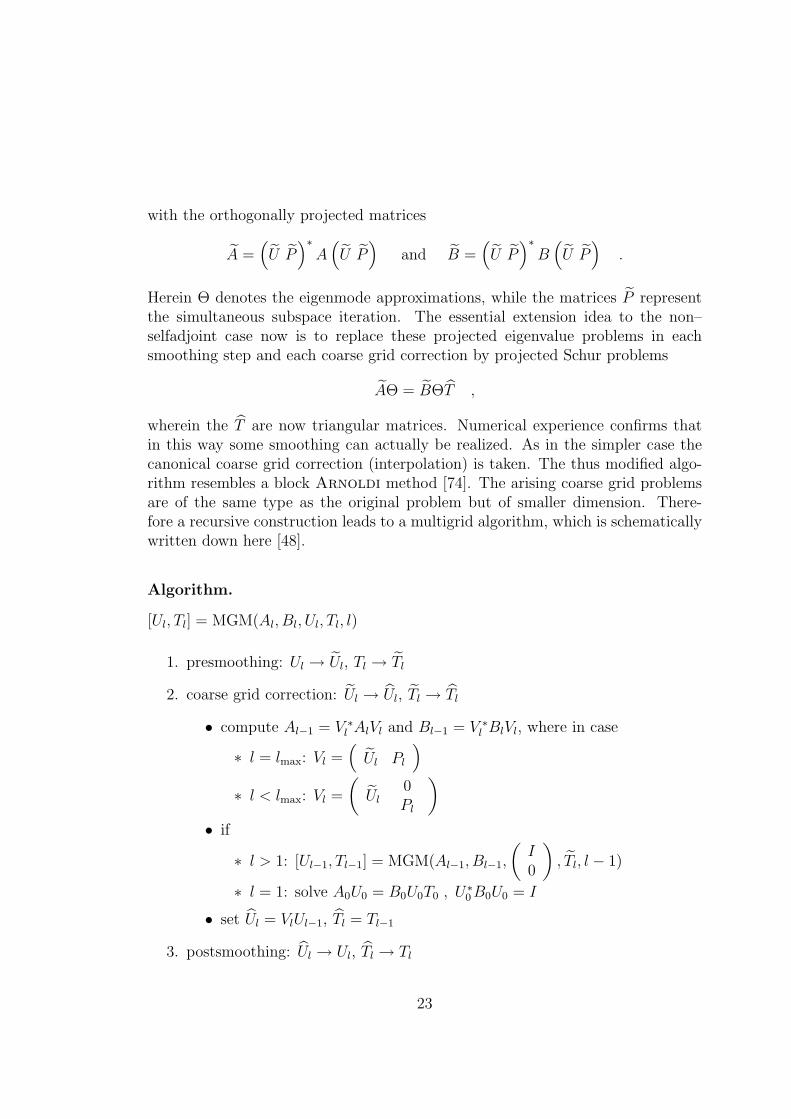
with the orthogonally projected matrices

A =(U P

)∗A

(U P

)and B =

(U P

)∗B

(U P

).

Herein Θ denotes the eigenmode approximations, while the matrices P representthe simultaneous subspace iteration. The essential extension idea to the non–selfadjoint case now is to replace these projected eigenvalue problems in eachsmoothing step and each coarse grid correction by projected Schur problems

AΘ = BΘT ,

wherein the T are now triangular matrices. Numerical experience confirms thatin this way some smoothing can actually be realized. As in the simpler case thecanonical coarse grid correction (interpolation) is taken. The thus modified algo-rithm resembles a block Arnoldi method [74]. The arising coarse grid problemsare of the same type as the original problem but of smaller dimension. There-fore a recursive construction leads to a multigrid algorithm, which is schematicallywritten down here [48].

Algorithm.

[Ul, Tl] = MGM(Al, Bl, Ul, Tl, l)

1. presmoothing: Ul → Ul, Tl → Tl

2. coarse grid correction: Ul → Ul, Tl → Tl

• compute Al−1 = V ∗l AlVl and Bl−1 = V ∗

l BlVl, where in case

∗ l = lmax: Vl =(

Ul Pl

)∗ l < lmax: Vl =

(Ul

0Pl

)• if

∗ l > 1: [Ul−1, Tl−1] = MGM(Al−1, Bl−1,

(I0

), Tl, l − 1)

∗ l = 1: solve A0U0 = B0U0T0 , U∗0 B0U0 = I

• set Ul = VlUl−1, Tl = Tl−1

3. postsmoothing: Ul → Ul, Tl → Tl

23

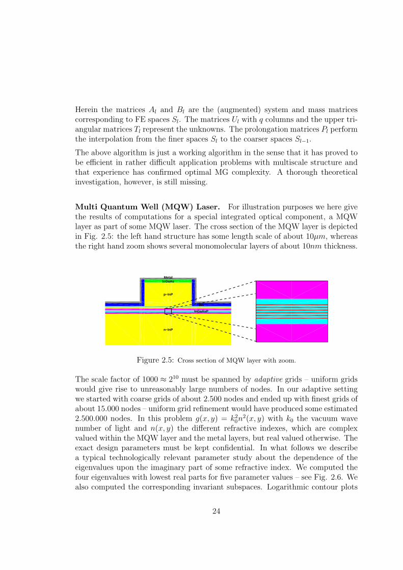
Herein the matrices Al and Bl are the (augmented) system and mass matricescorresponding to FE spaces Sl. The matrices Ul with q columns and the upper tri-angular matrices Tl represent the unknowns. The prolongation matrices Pl performthe interpolation from the finer spaces Sl to the coarser spaces Sl−1.

The above algorithm is just a working algorithm in the sense that it has proved tobe efficient in rather difficult application problems with multiscale structure andthat experience has confirmed optimal MG complexity. A thorough theoreticalinvestigation, however, is still missing.

Multi Quantum Well (MQW) Laser. For illustration purposes we here givethe results of computations for a special integrated optical component, a MQWlayer as part of some MQW laser. The cross section of the MQW layer is depictedin Fig. 2.5: the left hand structure has some length scale of about 10μm, whereasthe right hand zoom shows several monomolecular layers of about 10nm thickness.

MetalInGaAs

SiN

p−InP

InGaAsP

n−InP

Figure 2.5: Cross section of MQW layer with zoom.

The scale factor of 1000 ≈ 210 must be spanned by adaptive grids – uniform gridswould give rise to unreasonably large numbers of nodes. In our adaptive settingwe started with coarse grids of about 2.500 nodes and ended up with finest grids ofabout 15.000 nodes – uniform grid refinement would have produced some estimated2.500.000 nodes. In this problem g(x, y) = k2

0n2(x, y) with k0 the vacuum wave

number of light and n(x, y) the different refractive indexes, which are complexvalued within the MQW layer and the metal layers, but real valued otherwise. Theexact design parameters must be kept confidential. In what follows we describea typical technologically relevant parameter study about the dependence of theeigenvalues upon the imaginary part of some refractive index. We computed thefour eigenvalues with lowest real parts for five parameter values – see Fig. 2.6. Wealso computed the corresponding invariant subspaces. Logarithmic contour plots

24

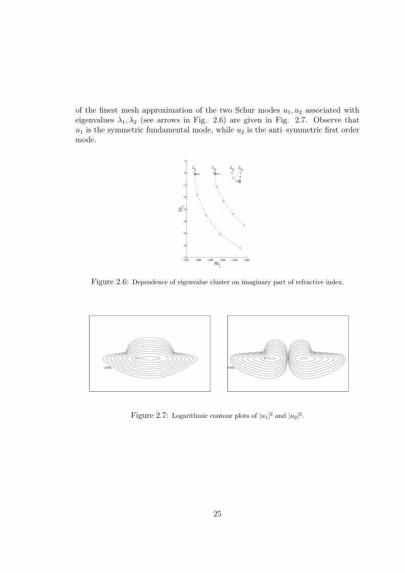
of the finest mesh approximation of the two Schur modes u1, u2 associated witheigenvalues λ1, λ2 (see arrows in Fig. 2.6) are given in Fig. 2.7. Observe thatu1 is the symmetric fundamental mode, while u2 is the anti–symmetric first ordermode.

−247 −246 −245 −244 −243 −242−7

−6

−5

−4

−3

−2

−1

0

1

ℜλj

ℑλ j

λ1

λ2

λ3

λ4

← ←

Figure 2.6: Dependence of eigenvalue cluster on imaginary part of refractive index.

0.7

0.001

0.7

0.001

Figure 2.7: Logarithmic contour plots of |u1|2 and |u2|2.

25

3 Countable Ordinary Differential Equations in

Polymer Industry

Chemically speaking, polymers are a special kind of macromolecules: chains ofsimple molecules or molecular groups, the monomers. The chains typically consistof ten thousand up to ten million monomers, say, and may be linear (the simplercase to be treated here) or even bifurcating. Copolymers are built from more thanone type of monomer. Polymer materials include a variety of synthetic materialssuch as lacquers, adhesives, PVC, and MMA. Mathematically speaking, models ofpolyreaction kinetics involve a huge set of ordinary differential equations (ODEs),usually nonlinear and stiff. The numbers of ODEs again range from ten thousandup to ten million – one per each arising polymer length. For a mathematicianit is simpler to think of countably infinitely many ODEs to be called countableODEs or just CODEs. Even though CODEs are usually underrated if not totallyoverlooked in standard mathematical textbooks on differential equations, they playan important role in several scientific fields, e.g. in environmental science (sootformation), astrophysics (cosmic dust), or medicine (pharmacokinetics). In thissection we will first describe the CODE models of typical polyreaction mechanisms.A survey of the basic computational approaches will follow. In more detail, wewill then present the recent concept of adaptive discrete Galerkin methods. Thisconcept has been first proposed in [45] by the author and Wulkow, who has thenimproved the method considerably in his thesis [87]. On this mathematical andsoftware basis he had started a spin–off firm, which – after the usual critical initialphase – meanwhile consults in chemical industry and research labs all over theworld.

3.1 Polyreaction Kinetics

In order to convey an impression of the CODE problem class, we begin with a shortlist of polyreaction mechanisms that arise in industrial applications. Only underunrealistic simplifications few of these CODEs can be solved in closed analyticform. In industrial applications, however, the mechanisms arise within combina-tions, which makes an analytical treatment anyway hopeless. That is why tworealistic problems are also included here in some detail. As for the notation, letPs(t) be the concentration of polymers of chain length or polymer degree s at timet. For ease of writing, we will not distinguish between the chemical species Ps, itsconcentration Ps(t), and the chain length distribution {Ps(t)}s=1,2..., but just relyon the context.

26

Chain addition polymerization or free radical polymerization. WithM(t) denoting some monomer concentration, this special reaction mechanism is

Ps + Mkp−→ Ps+1, s = 1, 2, . . . , (3.1)

where kp > 0 is the reaction rate coefficient. The kinetics of this reaction ismodeled by

P ′1 = kpMP1

P ′s = kpM(Ps − Ps−1), s = 2, 3, . . .

M ′ = kpM∞∑

s=1

Ps

(3.2)

with the given initial values

P1(0) = P10, Ps(0) = 0, s = 2, 3, . . . , M(0) = M0 . (3.3)

Coagulation and irreversible polycondensation. This mechanism can bedescribed in chemical terms as

Ps + Pr −→ Ps+r (3.4)

and modeled mathematically by the nonlinear CODE

P ′s =

1

2

s−1∑r=1

kr,s−rPrPs−r − Ps

∞∑r=1

ksrPrs s = 1, 2, . . . . (3.5)

Once again, the initial distribution Ps(0) is usually given.

Example: Biopolymerization [22]. This problem deals with an attempt torecycle waste of synthetic materials in an ecologically satisfactory way – whichis certainly an important problem of modern industrial societies. An attractiveidea in this context is to look out for synthetic materials that are both producedand eaten by bacteria – under different environmental conditions, of course. Aschematic illustration of the production process within such a bacterial recyclingis given in Fig. 3.1: there certain bacteria use fructose as a chemical input toproduce polyester (PHB) as chemical output. The macromolecular reaction steps

27

polyestersugar

Figure 3.1: Biopolymerization: bacteria eat sugar and produce polyester. White areas: poly-ester granules within bacteria cells.

of production and degradation of PHB can be summarized in the chemical model

Eka−→ A

A + Mki−→ P1

Ps + Mkp−→ Ps+1

Pskt−→ Ds + E

Ds+rkd−→ Ds + Dr

with s, r = 1, 2, . . . . Herein M denotes the monomer fructose, E an enzyme, A theactivated enzyme, Ps the so–called “living” and Ds the so–called “dead” PHB–polymer. The mathematical model for the above process comprises the CODEsystem

E ′ = −kaE + kt

smax∑r=1

Pr

A′ = +kaE − kiAM

M ′ = −kpM

smax∑r=1

Pr − kiAM

P ′1 = −kpMP1 + kiAM − ktP1

P ′s = −kpM(Ps − Ps−1) − kdPs , s = 2, 3, . . . , smax

D′s = +ktPs − kd(s − 1)Ds + 2kd

smax∑r=s+1

Dr , s = 1, 2, . . . , smax.

28

Herein the truncation index smax is not known a priori, practical considerationslead to roughly smax = 50.000 – which means that the above system consists of100.000 ODEs, each of which has roughly the same number of terms in the rightside.

Copolymerization. Most industrial synthetic materials are copolymers, typi-cally consisting of three up to seven different sorts of monomers. The mathematicalmodelling of such systems is often performed in terms of some multidimensionsalansatz Psr... with s monomers of type A, r monomers of tape B etc. This ansatz,however, leads to an enormous blowup in terms of both computing time and stor-age. An alternative model has been suggested in the chemical literature (see [46] forreference). In this approach polymers are characterized by their chemically activesite at one end of the chain. In the process of numerical solution of the polyre-action CODE enough information about these active sites comes up anyway. Inthis much simpler framework the following questions of chemical and economicalrelevance can still be answered: Which portion of the monomer is consumed in thecourse of the reaction? What are the time dependent relative distributions of thedifferent polymers? A typical example with three monomers will be given at theend of Section 3.3 below.

3.2 Basic Computational Approaches

As exemplified in the previous Section 3.1, CODE initial value problems are ingeneral infinite sets of nonlinear ODEs like

P ′s(t) = fs(P1(t), . . . , Ps(t), Ps+1(t), . . . ) , s = 1, . . . (3.6)

given together with initial values Ps(0). Whenever the above right hand side fs

contains only arguments up to Ps, i.e. it has the form fs(P1(t), . . . , Ps(t)), thenthe system can, in principle, be solved one by one – a property called self–closingin the literature. If fs has the general form as above, then it is said to be open.The latter case is the typical one in real life applications. In what follows we willsurvey and assess the basic algorithmic concepts for the numerical solution of openCODEs.

Direct numerical integration. In not too complicated cases direct stiff inte-gration of the reaction kinetics ODEs is still a popular approach. In fact, the authorand former co–workers have developed the efficient software package LARKIN (for

29

LARge chemical KINetics) to tackle such systems, see [6]. Typically, with any suchpackage, a sequential process is performed starting from a small number of ODEsand successively running up to larger and larger numbers. However, compared todirect integration even in this restricted application, the method to be presentedin Section 3.3 has proved computational speed–up factors of more than 10.000 to-gether with better accuracies for quantities of industrial relevance – compare [46].Finally, since all stiff integrators require the Jacobian matrix of the right hand side,this approach suffers from a rather narrow domain of applicability, just think ofthe 100.000 by 100.000 nonzero Jacobian elements in the above biopolymerizationexample.

Lumping technique. In this kind of technique linear combinations of compo-nents are collected to certain supercomponents, for which then ODEs are derivedand solved numerically. A proper collection of components requires a lot of a–prioriinsight into the process under consideration, sometimes just a log(s)–equilibrationis imposed. However, even though this technique is reported to work satisfactorilyin some linear ODE cases, it is certainly totally unreliable for nonlinear ODEs,which represent the bulk of industrially relevant models.

Method of statistical moments. The canonical formulation for distributions– like Ps(t) here – is in terms of statistical moments

μk(t)[P ] :=∑s≥1

skPs(t), k = 0, 1, . . . , .

Note that mass conservation shows up as μ0(t) = const. Insertion of the above de-finition into a polyreaction CODE (see Section 3.1 above) generates an infinite setof ODEs for these moments, a CODE again. It is easy to show that the structuralproperty open/selfclosing of the original polyreaction CODE is passed on to themoment CODE. The whole approach is based on the theorem of Stieltjes, whichstates that the knowledge of all moments (if they are bounded) is equivalent tothe knowledge of the distribution. If, however, only a finite number N of momentsis known, in practice mostly only few moments, then there exists a full range ofapproximations P

(N)s with unclear representation and approximation quality.

One popular method to deal with this lack of information is to specify the distrib-ution in advance. For example, assume that – on the grounds of scientific insightinto the given problem – the unknown distribution is expected to be a Poisson

30

distribution

Ps = C e−λs λs−1

(s − 1)!,

then the unknown parameters λ, C can be determined from just the two moments

C = μ0, λ =μ1

μ0

.

Once the two moments are computed, the distribution as a whole seems to beknown. Sometimes this kind of specification is also hidden behind so–called closurerelations. However, strictly speaking, none of these approaches can assure that thestated problem is really solved – without further check of whether the assumptionsmade are appropriate. An insidious feature of any such approach is that all thethus computed approximations look optically smooth and therefore “plausible” –even when they are totally wrong! That is why these two approaches are onlyrecommended for situations wherein the essential features of the solution are well–studied.

Last but not least, it is not clear how many terms need to be kept in the trun-cated moment CODE. Of course, the approximate moments μ

(N)k corresponding to

truncation index N should be accurate enough within some prescribed tolerancecompared to the exact moments μk. The choice of truncation index N becomeseven hopeless when the reaction rate coefficients depend on the chain length – ase.g. in soot formation, cf. [45, 88].

Monte Carlo method. Markov chains play some role in the computation ofstationary solutions of copolymerization problems. In the application studied here,however, Monte Carlo methods require too much computing time in comparisonwith the method to be presented in Section 3.3. They will play an important rolein Section 4.2 below in some different context.

Galerkin methods for continuous PDE models. A rather popular approachto condense the infinite number of ODEs is to model the degree s by some realvariable, interpreting sums as infinite integrals and thus arriving at integro–partialdifferential equations, usually with lag terms (like e.g. the neutron transport equa-tion). Following this line, an unknown modelling error for low s is introduced –which is the very part of the models where measurements are typically available.Moreover, depending on the polyreaction mechanism, the arising problem mayturn out to be ill–posed, which in turn requires some regularization to be carefully

31

studied. In [49], Gajewski/Zacharias suggested Galerkin methods in Hilbertspace based on modified Laguerre polynomials Lα

k for the weight function

Ψ(s) = σαe−σ with σ = β(t)s, β =μ0(t)

μ1(t). (3.7)

The specification of β assures scaling invariance in the (continuous) variable s.

Discrete Galerkin methods for CODEs. In [45] the author had suggested touse the above PDE approach only in principle, but to avoid turning the discretevariable s artificially into a continuous one. Upon interpreting discrete inner prod-ucts as infinite sums, the discrete nature of the problem can be preserved – thuskeeping the proper regularization. As a first attempt on this mathematical basis,discrete Galerkin methods based on discrete Laguerre polynomials lk for theweight function

Ψ(s) = ρs, ρ < 1 . (3.8)

were constructed. The specification of ρ via “scaling” of the argument as in (3.7)is not directly possible here, since for a discrete variable s scaling is not a properconcept (see, however, the “moving weight function” concept below). This discreteGalerkin approach turned out to be the starting point for the construction of anew class of rather efficient algorithms to be discussed in detail in the next section.

3.3 Adaptive Discrete Galerkin Methods

For ease of presentation we replace the above nonlinear CODE (3.6) by the linearCODE

P ′s(t) = (AP (t))s Ps(0) given . (3.9)

Herein the discrete operator A describing the polyreaction mechanisms may bebounded (rare) or, unbounded (typical). The key to the construction of discreteGalerkin methods is the introduction of a discrete inner product

(f, g) :=∞∑

s=1

f(s)g(s)Ψ(s) (3.10)

in terms of some prescribed componentwise positive weighting function Ψ. Thisproduct induces a set of orthogonal polynomials {lj}, j = 1, 2, . . . satisfying therelations

(lj, lk) = γjδjk , γj > 0 j, k = 0, 1, 2, . . . (3.11)

32

For the solution P of the CODE we naturally try the corresponding ansatz

Ps(t) = Ψ(s)∞∑

k=0

ak(t)lk(s). (3.12)

Moving weight function. There exists an interesting close connection betweenthe statistical moments μk and the just introduced coefficients ak. Upon represent-ing the monomials sk by the orthogonal set of polynomials, we are able to derivean infinite lower triangular system of algebraic equations of the form

μ0 = b00γ0a0,μ1 = b10γ0a0 + b11γ1a1,μ2 = . . . ,

(3.13)

where bkk = 0 is guaranteed. Herein the moments μk arise row–wise, whereas thecoefficients ak arise column–wise. This implies that if all moments are given andbounded, then all coefficients can be computed, which is just the already mentionedStieltjes theorem. If only N moments are given, then only N coefficients can becomputed. On the side of the coefficients, however, we have a reasonable optionof truncating the expansion (3.12), since they (unlike the moments) are knownto decrease asymptotically, if the solution P can actually be represented by theabove ansatz. In other words, the solution P must be contained in some weightedsequence space, say HΨ, with an associated inner product and its induced norm

< f, g >:=∞∑

s=1

f(s)g(s)/Ψ(s), ‖f‖2 :=< f, f > . (3.14)

In order to enforce that P ∈ HΨ throughout the whole evolution, we additionallyrequire that P ≈ μ0Ψ by imposing the moving weight function conditions

ν0[Ψ] = 1, ν1[Ψ] =μ1[P ]

μ0[P ](3.15)

wherein the νk denote the statistical moments of the prescribed weight function.The first condition means that Ψ is some probability density function, whereasthe second one assures some time dependent coupling of the mean values of theunknown distribution P to the known distribution Ψ – hence the name. Insertionof (3.15) into (3.13) leads to the two equivalent conditions

a0(t) = μ0(t), a1(t) = 0 (3.16)

33

independent of the underlying problem and of the choice of weight function. Sum-marizing, with these two additional conditions a much smaller number n of degreesof freedom turned out to be sufficient to characterize the dynamics of realisticpolyreaction systems.

Method of lines. Upon insertion of the expansion (3.12) into the CODE (3.9),multiplication by the test function lj(s), summation over s, change of summationorder, and use of the above orthogonality relations, we end up with the CODE

γja′j(t) =

∞∑k=0

ak(t)(lj,Alk) j = 0, 1, . . . . (3.17)

for the ak. In the above moving weight function approach the ODE for a1 canbe dropped (recall that a1 = 0) and a new ODE can be created instead, say, forthe parameter ρ in the discrete Laguerre method based on Ψ as in (3.8). Inother words, in this method of lines type approach the moving weight functioninduces a moving basis lk(s; ρ(t)), k = 0, 1, . . . – similar to moving nodes in PDEapplications with moving fronts.

For the numerical realization of (3.17), the inner products

(lj,Alk) =∞∑

s=1

lj(s)A(s)lk(s)Ψ(s)

must be approximated by a finite number of terms to prescribed accuracy. In rarecases analytical methods allow a closed form representation, which is cheap to eval-uate. In most cases, however, numerical approximations turn out to be the onlychoice. We developed two efficient approximation methods: an adaptive multi-grid summation technique (compare Section 9.7.2 in the undergraduate numericalanalysis textbook [35]), a discrete variant of the MG method described in Section1.1, and a Gauss–Christoffel summation, a discrete variant of Gauss–Christoffelquadrature based on the selected weight function Ψ. As for the applied timediscretization, linearly implicit schemes in the generally nonlinear CODEs (3.6)turned out to be efficient to tackle the unbounded part of the discrete Frechetoperators of the right hand side. In addition, adaptive timestep and order controlis as useful as in ordinary stiff integration.

Adaptive truncation. Truncation of this CODE by setting

aj = 0, j = n, n + 1, . . .

leads to the discrete Galerkin approximation

P (n)s (t) = Ψ(s)

n∑k=0

a(n)k (t)lk(s). (3.18)

34

In the simpler case of self–closing CODEs, the coefficients ak do not depend onthe truncation index n. The key to adaptivivity in any (global) Galerkin methodis that the truncation error can be estimated by∣∣P (n) − P

∣∣ .=

∣∣P (n) − P (n+1)∣∣ =[

(a(n)n+1)(t)

2γn+1 +∑n

k=0

(a

(n)k (t) − a

(n+1)k (t)

)2

γk

]12

.(3.19)

Note that if we want to assure a condition like∣∣P (n) − P (n+1)∣∣ ≤ TOL

for some prescribed error tolerance TOL, then we might thus obtain some timedependent number n(t) of terms in the Galerkin approximation.

Adaptive Rothe method. As already tacitly indicated in the above movingweight function conditions, the typical CODE initial value problem lives in somescale of Hilbert spaces, say Hρ(t), t ≥ t0 for the discrete Laguerre method, ratherthan just in single fixed space. This nicely shows up in a special Lipschitz condition,a nonlinear extension of a semi–continuity assumption:

‖f(t, u) − f(t, v)‖ρ ≤ M

(ρ − ρ)γ‖u − v‖ρ, 0 < γ ≤ 1,

ρ > ρ and u, v ∈ Hρ .(3.20)

This condition is the essential ingredient of a uniqueness theorem for CODEs – see[87]. In analogy to the discussion for PDEs in Section 1.1 above, the appropriateorder of discretization will therefore be first time discretization, then Galerkinapproximation, which is the so–called Rothe method. Starting from some initialvalue u(t) = φ suppose we apply some linearly implicit Euler discretization

(I − τA)Δu = τf(ϕ) , u1 = ϕ + Δu , (3.21)

wherein A is the derivative fu(ϕ). This is a linear boundary value problem in somediscrete sequence space to be treated numerically by a discrete Galerkin method.The numerical realization of the time step control requires an estimate η1 of theerror ‖u1−u(t+ τ)‖ in the norm ‖ · ‖ induced by the corresponding inner product.For this purpose we solve the correction equation

(I − τA)η1 = −1

2τ 2Af(ϕ) , u2 = u1 + η1 , (3.22)

35

which obviously has the same structure as (3.21). The approximation u2 is of order2 in time, which implies the estimated optimal time step (with safety factor σ < 1)

τnew = τ

√στtol

‖η1‖. (3.23)

In this realization the truncation index for (3.22) may correspond to a less strin-gent (absolute) error tolerance than the one for (3.21), since (3.23) requires lessaccuracy; in this setting the approximation u1 is regarded as the accepted solution.If the same absolute accuracy is prescribed in both equations, then u2 is taken asthe accepted approximation.

Discrete h-p–method. For sufficiently complex problems in industry globalGalerkin methods – such as the one given in (3.12) – have meanwhile been clearlyoutperformed by local Galerkin methods (similar as FEMs in PDEs). In order tobe able to construct local multilevel bases, the weight function has to be restrictedto Ψ = 1 on finite subintervals, which induce (discrete) Chebyshev polynomialstk of degree k. The actually developed method combines adaptive interval refine-ment (h–method) with adaptive choice of the local degree (p–method) to obtainsome rather sophisticated adaptive h-p–method on some finite interval. In orderto match the asymptotic tail of the distribution, global representations still play arole.

In the course of the years the successive efficient treatment of industrially relevantpolyreaction problems has led to a steady increase of modern rather sophisti-cated algorithmic tools that made their way into the commercial software packagePrediciTM of Wulkow [88]. The following copolymerization example with threemonomers should give some flavor of such problems.

Example: Radical terpolymerization [46]. Let Ps be the polymer with ac-tive end MMA (index a), Qs the one with styrole (index b), and Rs the one withMSA (index c below). With this notation, the chemical reaction scheme reads

Initialization:

Ikd−→ 2I∗

I∗ + MMAkl−→ P ∗

1

I∗ + Skl−→ Q∗

1

I∗ + MSAkl−→ R1

36

Chain growth:

P ∗s + MMA

kpaa−→ P ∗s+1

P ∗s + S

kpab−→ Q∗s+1

P ∗s + MSA

kpac−→ R∗s+1

Q∗s + MMA

kpba−→ P ∗s+1

Q∗s + S

kpbb−→ Q∗s+1

Q∗s + MSA

kpbc−→ R∗s+1

R∗s + MMA

kpca−→ P ∗s+1

R∗s + S

kpcb−→ Q∗s+1

Chain termination:

P ∗s + P ∗

rkcaa−→ Ds+r

P ∗s + Q∗

r

kcab−→ Ds+r

Q∗s + Q∗

r

kcbb−→ Ds+r

For reasons of confidentiality some parts of the mechanism are left out. Initialvalues and generic reaction rate coefficients are given in [46]. Under the modellingassumption that in this specific polymerization process the living chains live onlyfor a very short time span, the copolymer distribution can be computed as follows.Define e.g. integrated quantities like

Ps(t) =

∫ t

0

Ps(t)dt .

which (up to normalization) counts the number of coplymers with MMA in fixedposition s. Then the relation Ps : Qs : Rs offers detailed insight into the composi-tion of the copolymer. In Fig. 3.2 such compositions are shown for times t = 360min and t = 1.080 min. Information of this kind could not have been gained fromstatistical moment analysis as applied earlier in industry.

37

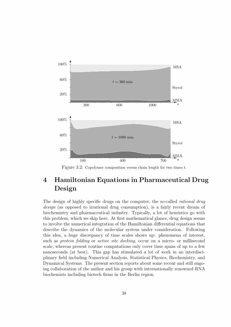
20%

60%

100%

200 600 1000

Styrol

MMA

MSA

s

t = 360 min

20%

60%

100%

100 400 700

Styrol

MMA

MSA

t = 1080 min

s

Figure 3.2: Copolymer composition versus chain length for two times t.

4 Hamiltonian Equations in Pharmaceutical Drug

Design

The design of highly specific drugs on the computer, the so-called rational drugdesign (as opposed to irrational drug consumption), is a fairly recent dream ofbiochemistry and pharmaceutical industry. Typically, a lot of heuristics go withthis problem, which we skip here. At first mathematical glance, drug design seemsto involve the numerical integration of the Hamiltonian differential equations thatdescribe the dynamics of the molecular system under consideration. Followingthis idea, a huge discrepancy of time scales shows up: phenomena of interest,such as protein folding or active site docking, occur on a micro- or millisecondscale, whereas present routine computations only cover time spans of up to a fewnanoseconds (at best). This gap has stimulated a lot of work in an interdisci-plinary field including Numerical Analysis, Statistical Physics, Biochemistry, andDynamical Systems. The present section reports about some recent and still ongo-ing collaboration of the author and his group with internationally renowned RNAbiochemists including biotech firms in the Berlin region.

38

Our special contribution to drug design starts from the known insight that thecorresponding trajectories are chaotic, which means that small perturbations ofthe initial values of such trajectories asymptotically lead to unbounded deviations.In terms of Numerical Analysis this means that the Hamiltonian initial valueproblems (IVPs) are ill–conditioned after short time spans. On the basis of thisinsight, we suggested a novel concept for the computation of essential features ofHamiltonian dynamical systems. The key idea presented in Section 4.1. below isto directly compute chemical conformations and rates of conformational changes,interpreting chemical conformations as almost invariant sets in the phase space(positions and momenta) of the corresponding dynamical system. In a first step,this led to an eigenproblem for eigenvalue clusters around the Perron root of theso-called Frobenius-Perron operator associated with the (numerical) flux ofthe dynamical system.

In a second step, in Section 4.2., we interpreted chemical conformations as objectsin the position space of the Hamiltonian dynamical system. Moreover, we aban-doned the deterministic Hamiltonian systems with given initial values to turn overto ensembles of initial values in the frame of Statistical Physics. This led to thenatural construction of a stochastic operator, which appears to be selfadjoint oversome weighted L2-space. Discretization of that operator by means of certain hy-brid Monte Carlo methods (HMC) generates nearly uncoupled Markov chains thatneed to be computed. As it turns out, the eigenvectors associated with the Perroncluster of eigenvalues for the stochastic operator contain the desired informationabout the chemical conformations and their patterns of change.

The described approach is presently worked out in collaboration with biochemiststhat design RNA drugs in their chemical labs. Our aim is to substitute timeconsuming and costly experiments in the chemical RNA lab by reliable simulationsin a virtual RNA Lab. First steps in this direction are illustrated in Section 4. 3at some fairly complex, but moderate size RNA molecule.

4.1 Deterministic Chaos in Molecular Dynamics

In classical textbooks on Molecular Dynamics (MD), see e.g. [1], a single moleculeis modelled by a Hamilton function

H(q, p) = 12pT M−1p + V (q) (4.1)

with q the 3D atomic positions, p the (generalized) momenta, M the diagonalmass matrix, and V a differentiable potential function. The Hamilton function iscalled separated, whenever the p-part and the q-part of H are separated as above.

39

The Hamilton function defined on the phase space Γ ⊂ R6N induces the canonicalequations of motion, the Hamiltonian equations

q = M−1p, p = −grad V , (4.2)

which describe the dynamics of the molecule in a deterministic way: For giveninitial state x0 = (q(0), p(0)) the unique formal solution of (4.2) is usually writtenas x(t) = (q(t), p(t)) = Φtx0 in terms of the flow Φt. Numerical integration of (4.2)by any one-step method with stepsize τ leads to the discrete solution

xk+1 = Ψτxk ⇒ xk = (Ψτ )k x0, (4.3)

in terms of a discrete flow Ψτ .

Condition of the initial value problem. Given an initial perturbation δx0 weare interested in its growth along the flow

δx(t; x0) = Φt(x0 + δx0) − Φtx0 .

The condition number κ(t) of an initial value problem (see the textbook by Deufl-

hard and Bornemann [32]) may be defined as the worst case error propagationfactor in first order perturbation analysis so that (in some suitable norm | · |)

|δx(t; x0)| < κ(t)|δx0| for all x0.

It is of utmost importance to keep in mind that κ(t) is a quantity characterizingthe analytic problem independent of any discretization. A linear growth resultκ(t) ∼ t holds for a subclass of so–called integrable Hamiltonian systems such asthe popular Kepler problem – see Arnold [3]. In real life MD problems, however,κ increases exponentially. In order to illustrate this behavior, Fig. 4.1 shows resultsfor the simple Butane molecule. In order to be able to ignore any discretizationerror effects, unusually small time steps (τ = 0.005 fs) within the Verlet schemehave been chosen. A physically negligible initial perturbation 10−4A can be seen toovergrow the nominal solution after a time span T > 500 fsec, which is significantlyshorter than the time spans of physical interest.

Once long term trajectories in MD have been identified as ill-conditioned mathe-matical objects, they should be avoided in actual computation. Only short termtrajectories should be accepted as numerical input for further scientific interpre-tation. This seems to be in direct contradiction to the possible prediction of longterm behavior of biomolecules! How can we overcome this difficulty?

Warning. There are quite a number of beautiful movies about the dynamicsof biomolecules that visualize merely accidental numerical results of long termsimulations – and are therefore of doubtful value for chemical interpretation.

40

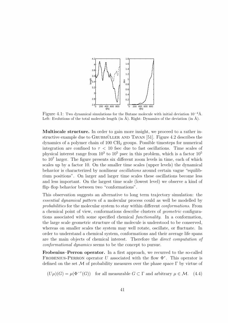
0 200 400 600 8002.6

2.8

3

3.2

3.4

3.6

3.8

4

4.2

t[fs]

leng

th

0 200 400 600 8000

0.2

0.4

0.6

0.8

1

1.2

1.4

1.6

1.8

t[fs]

dev

Figure 4.1: Two dynamical simulations for the Butane molecule with initial deviation 10−4A.Left: Evolutions of the total molecule length (in A). Right: Dynamics of the deviation (in A).

Multiscale structure. In order to gain more insight, we proceed to a rather in-structive example due to Grubmuller and Tavan [51]. Figure 4.2 describes thedynamics of a polymer chain of 100 CH2 groups. Possible timesteps for numericalintegration are confined to τ < 10 fsec due to fast oscillations. Time scales ofphysical interest range from 103 to 105 psec in this problem, which is a factor 105

to 107 larger. The figure presents six different zoom levels in time, each of whichscales up by a factor 10. On the smaller time scales (upper levels) the dynamicalbehavior is characterized by nonlinear oscillations around certain vague “equilib-rium positions”. On larger and larger time scales these oscillations become lessand less important. On the largest time scale (lowest level) we observe a kind offlip–flop behavior between two “conformations”.

This observation suggests an alternative to long term trajectory simulation: theessential dynamical pattern of a molecular process could as well be modelled byprobabilities for the molecular system to stay within different conformations. Froma chemical point of view, conformations describe clusters of geometric configura-tions associated with some specified chemical functionality. In a conformation,the large scale geometric structure of the molecule is understood to be conserved,whereas on smaller scales the system may well rotate, oscillate, or fluctuate. Inorder to understand a chemical system, conformations and their average life spansare the main objects of chemical interest. Therefore the direct computation ofconformational dynamics seems to be the concept to pursue.

Frobenius–Perron operator. In a first approach, we recurred to the so-calledFrobenius-Perron operator U associated with the flow Φτ . This operator isdefined on the set M of probability measures over the phase space Γ by virtue of

(Uμ)(G) = μ(Φ−τ (G)) for all measurable G ⊂ Γ and arbitrary μ ∈ M. (4.4)

41

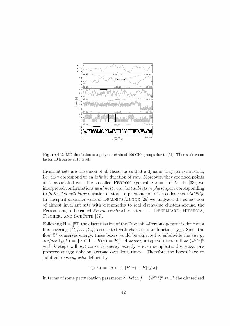
Figure 4.2: MD simulation of a polymer chain of 100 CH2 groups due to [51]. Time scale zoomfactor 10 from level to level.

Invariant sets are the union of all those states that a dynamical system can reach,i.e. they correspond to an infinite duration of stay. Moreover, they are fixed pointsof U associated with the so-called Perron eigenvalue λ = 1 of U . In [33], weinterpreted conformations as almost invariant subsets in phase space correspondingto finite, but still large duration of stay – a phenomenon often called metastability.In the spirit of earlier work of Dellnitz/Junge [29] we analyzed the connectionof almost invariant sets with eigenmodes to real eigenvalue clusters around thePerron root, to be called Perron clusters hereafter – see Deuflhard, Huisinga,

Fischer, and Schutte [37].

Following Hsu [57] the discretization of the Frobenius-Perron operator is done on abox covering {G1, . . . , Gn} associated with characteristic functions χGi

. Since theflow Φτ conserves energy, these boxes would be expected to subdivide the energysurface Γ0(E) = {x ∈ Γ : H(x) = E}. However, a typical discrete flow (Ψτ/k)k

with k steps will not conserve energy exactly – even symplectic discretizationspreserve energy only on average over long times. Therefore the boxes have tosubdivide energy cells defined by

Γδ(E) = {x ∈ Γ, |H(x) − E| ≤ δ}

in terms of some perturbation parameter δ. With f = (Ψτ/k)k ≈ Φτ the discretized

42

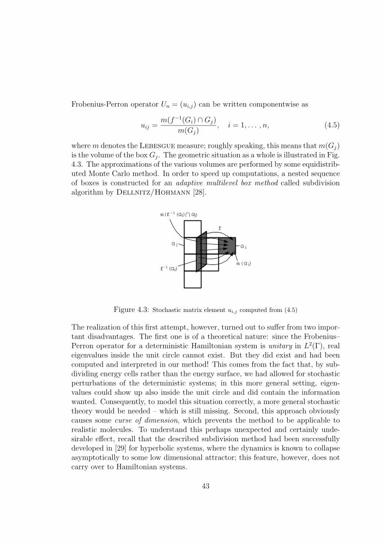
Frobenius-Perron operator Un = (ui,j) can be written componentwise as

uij =m(f−1(Gi) ∩ Gj)

m(Gj), i = 1, . . . , n, (4.5)

where m denotes the Lebesgue measure; roughly speaking, this means that m(Gj)is the volume of the box Gj. The geometric situation as a whole is illustrated in Fig.4.3. The approximations of the various volumes are performed by some equidistrib-uted Monte Carlo method. In order to speed up computations, a nested sequenceof boxes is constructed for an adaptive multilevel box method called subdivisionalgorithm by Dellnitz/Hohmann [28].

���

f

Gi

m(Gi)

Gj

f -1(Gi)

m(f -1(Gi) Gj)∩

Figure 4.3: Stochastic matrix element ui,j computed from (4.5)

The realization of this first attempt, however, turned out to suffer from two impor-tant disadvantages. The first one is of a theoretical nature: since the Frobenius–Perron operator for a deterministic Hamiltonian system is unitary in L2(Γ), realeigenvalues inside the unit circle cannot exist. But they did exist and had beencomputed and interpreted in our method! This comes from the fact that, by sub-dividing energy cells rather than the energy surface, we had allowed for stochasticperturbations of the deterministic systems; in this more general setting, eigen-values could show up also inside the unit circle and did contain the informationwanted. Consequently, to model this situation correctly, a more general stochastictheory would be needed – which is still missing. Second, this approach obviouslycauses some curse of dimension, which prevents the method to be applicable torealistic molecules. To understand this perhaps unexpected and certainly unde-sirable effect, recall that the described subdivision method had been successfullydeveloped in [29] for hyperbolic systems, where the dynamics is known to collapseasymptotically to some low dimensional attractor; this feature, however, does notcarry over to Hamiltonian systems.

43

4.2 Identification of Metastable Conformations

This section describes a rather recent improved approach mainly due to Schutte

[80, 81]. This approach keeps the conceptual advantages of the Dynamical Systemsapproach (as given in Section 4.1), but avoids the conceptual disadvantages by ex-ploiting concepts of Statistical Physics instead. Its key new feature is the replace-ment of the Frobenius-Perron operator by some well-designed Markov operator,a spatial transition operator based on Boltzmann statistics. Most experimentsin a chemical lab are performed under the conditions of constant temperature andvolume, which is known to give rise to the canonical density

f0(x) =1

Zexp (−β H(x)) , with Z =

∫Γ

exp (−β H(x)) dx, (4.6)

where β = 1/kBT , temperature T , and Boltzmann’s constant kB.

We start with some notion of almost invariant sets in the language of statistics.For some selected set S let χS denote its characteristic function, i.e. χS(x) = 1iff x ∈ S and χS(x) = 0 otherwise. Then the transition probability between twosubsets S1, S2 of the phase space Γ is given by

w(S1, S2, τ) =1∫

S1f0(x) dx

∫S1

χS2(Φτx) f0(x) dx S1, S2 ⊂ Γ (4.7)

By this definition almost invariant sets will be those with w(S, S, τ) ≈ 1. In Section4.1 we had understood chemical conformations as almost invariant sets in phasespace. However, in reality these objects are observed in position space. That iswhy we now turn over to characterize conformations as sets B in position spaceΩ ⊂ R3N . Upon allowing for arbitrary momenta p, we are naturally led to focusour interest on the phase space fiber

Γ(B) = {(q, p) ∈ Γ, q ∈ B} . (4.8)

With this notation we now call a set B ⊂ Ω a conformation whenever

w(Γ(B), Γ(B), τ) ≈ 1. (4.9)

For H separable as in (4.1), f0 from (4.6) splits into the product

f0(x) =1

Zp

exp

(−β

2pT M−1p

)︸ ︷︷ ︸

=P(p)

1

Zq

exp (−β V (q))︸ ︷︷ ︸=Q(q)

, (4.10)

44

with P and Q normalized such that∫P(p)dp =

∫Q(q)dq = 1.

Upon returning to (4.8), we may specify the conditional probability for a systembeing in set B ⊂ Ω to move to set C ⊂ Ω after some time τ as

w(Γ(B), Γ(C), τ) =1∫

Γ(B)

f0(x) dx

∫Γ(B)

χΓ(C)(Φτx) f0(x) dx . (4.11)

Construction of spatial Markov operator. With these preparations we arenow ready to confine all terms to position space only. The denominator in (4.11)represents the probability for a system from the statistical ensemble to be withinB ⊂ Ω which can be simplified using dx = dqdp (for H separable) and the nor-malization of P to yield

π(B) =

∫Γ(B)

f0(x) dx =

∫B

Q(q) dq . (4.12)

The analog treatment of the numerator in (4.11) will give rise to the definition ofan operator T . Let ξ1(q, p) = q denote the projection from the variables x to theposition variables and introduce an inner product in the weighted Hilbert spaceL2Q by

〈u, v〉Q =

∫Ω

u∗(q) v(q)Q(q) dq

together with its induced norm

‖u‖2Q = 〈u, u〉Q .

With this notation we may write∫Γ(B)

χΓ(C)(Φτx) f0(x) dx =

∫C

{∫R3N

χB(ξ1Φτ (q, p))P(p) dp

}Q(q) dq

︸ ︷︷ ︸=: 〈TχB ,χC〉Q

(4.13)

thus defining the operator

Tu(q) =

∫u(ξ1Φ

τ (q, p))P(p) dp, (4.14)

45

Upon combining (4.11) up to (4.13) we may write the conditional probability of asystem being in B to move into C during time τ as

w(B, C, τ) =〈TχB, χC〉Q

π(B)B, C ⊂ Ω (4.15)

By construction, T can be interpreted as the restriction of the Frobenius–Perronoperator U , see (4.4), to position space via averaging over the momentum part ofthe canonical distribution. The operator T is defined on the weighted spaces

LrQ(Ω) = {u : Ω → C,

∫Ω

|u(q)|rQ(q) dq < ∞}, r = 1, 2.

In terms of these spaces the important properties of T are (Schutte [80]):

1. T is bounded in LpQ(Ω): ‖Tu‖Q ≤ ‖u‖Q p = 1, 2

2. T is a Markov operator on L1Q(Ω).

3. T is selfadjoint in L2Q, since Φτ is reversible. Hence, the spectrum σ(T ) is

real-valued and bounded: σ(T ) ⊂ [−1, 1].

4. There exists a Perron cluster of discrete eigenvalues well-separated from theremaining (continuous) part of the spectrum.

Properties 1-3 hold for Hamiltonian systems in general; property 4 only holdsunder additional assumptions – which are, however, satisfied in the systems ofinterest here. Summarizing, T has just the theoretical properties needed as a basisfor the computational identification of conformational subsets via the eigenmodesto Perron clusters of eigenvalues.

Discretization of Markov operator. We proceed as in the previous section byintroducing a set of boxes, this time in position space rather than phase space. Let{G1, . . . , Gn} ⊂ Ω denote a covering of Ω. In view of a Galerkin approximationin L2

Q we define the basis Vn = span{χ1, . . . , χn} in terms of the characteristicfunctions χi = χGi

. Moreover, let π(Gi) = πi. In this basis we may construct an(n, n)-matrix P = (pij) via spatial transition probabilities as

pij =〈Tχi, χj〉Q

πi

= w(Gi, Gj, τ) i, j ∈ {1, . . . , n}. (4.16)

By construction, this matrix P is row-wise stochastic and, since T is self-adjoint,also reversible. Upon observing the condition of detailed balance in the form

πi pij = πj pji, ∀i, j ∈ {1, . . . , n}.

46

the matrix is symmetric with respect to a weighted discrete inner product, whichimplies that σ(P ) ⊂ [−1, 1], real. Moreover, there exists a Perron cluster of eigen-values, if the boxes are well-chosen to really cover the relevant position space.

Hybrid Monte Carlo realization. The above introduced Markov operator Tin L1

Q(Ω) can also be interpreted as a transition operator that generates a Markov

chain {qk}k=0,1,... via the discrete stochastic dynamical system

qk+1 = ξ1Φτ (qk, pk), k = 0, 1, . . . , (4.17)

wherein the momenta pk in each step are chosen randomly from the distributionP . Obviously, upon changing from the Frobenius-Perron operator U to the transi-tion operator T , we also change from the discrete deterministic dynamical system(4.3) to its stochastic counterpart (4.17). Iterations of (4.17) realize sequences{qk} that are asymptotically distributed according to Q. This feature can be ex-ploited by application of suitable Monte Carlo (MC) methods. After M samples{qj} from (4.17) the Q-expectation value of any spatial observable A : Ω → R isapproximated by an averaged sum such that

∣∣∣ 1

M

M∑j=1

A(qj) −∫Ω

A(q)Q(q) dq∣∣∣ ≤ C M−1/2, (4.18)

with a constant C not explicitly depending on dim(Γ) = 6N . In the present con-text, the observable will be any of the 1

2n(n+1) integrand factors Tχiχj arising in

(4.16). As the integrand contains the (short term numerical) flux, a hybrid MonteCarlo (HMC) method is preferably applied, which is a compromise between trajec-tory evaluation and MC. In more detail, the matrix elements pij are asymptoticallyapproximated by virtue of relative frequencies

# (qk ∈ Gi ∧ qk+1 ∈ Gj)

# (qk ∈ Gi)→ w(Gi, Gj, τ) = pij i, j ∈ {1, . . . , n}. (4.19)

The theoretical result (4.18) raises the expectation that we have eventually over-come the curse of dimension. However, the well-known undesirable effect of criticalslowing down of the iteration due to local trapping is still possible. For this rea-son, we developed an adaptive temperature variant called ATHMC – see Fischer,

Cordes, and Schutte [47].

Essential degrees of freedom. In realistic RNA drug molecules we have to facearound N > 100 atoms – see Fig. 4.5. If we subdivide each of the 3N state variablesinto m pieces, then the dimension of the stochastic matrix P would be n = m3N

– which would be just too much even for a Krylov space iterative eigenproblem

47

solver. Therefore, in the spirit of a suggestion due to Amadei, Linssen, and

Berendsen [2], we start with a long term HMC series and apply some covarianceanalysis to it; this technique then helps to reduce the total number of state variablesto a subset of d << 3N essential variables so that only n = md discretization boxesare needed. A realistic example will be presented in the subsequent Section 4.3.

Eigenvalue Cluster analysis. Assume that we know how to evaluate the entriesof P . So we are finally left with the numerical solution of the eigenproblem

Pα = λα with α = (α1, . . . , αn) .

for a cluster of eigenvalues around the Perron eigenvalue λ = 1. One question isthat we will not know in advance how many of the eigenvalues close to 1 should beincluded into the Perron cluster. The basic insight from [37] is that the k eigen-values in the Perron cluster should be interpretable as a perturbed k-fold Perronroot. The decision about k is quite subtle and has to be made by careful exami-nation of the matrix W defined below in (4.22). Suppose now that this decisionhas been made. Then the conformational sets can be computed via appropriatelinear combinations of the eigenmodes corresponding to the Perron cluster. Eachconformation, say B, is represented as a set of indices, say IB, that mark the as-sociated boxes belonging to the spatial conformation. Given such a conformationas subset B ⊂ Ω, the probability for the dynamical system to stay within B caneasily be evaluated via the relation

w(B, B, τ) =1∑

i∈IB

πi

∑i,j∈IB

πi pij . (4.20)

This should be distinguished from the probability for the system to be within aconformation (compare also (4.12))

π(B) =∑i∈IB

πi . (4.21)

Finally, with k conformations B1, B2, . . . , Bk identified, the transition rates be-tween conformations can be arranged in the (k, k)–matrix

W = (wij) =(w(Bi, Bj, τ)

), i, j = 1, . . . , k (4.22)

which, together with the vector {π(B1), . . . , π(Bk)}, contains the core informationof conformation dynamics. Details of this Perron cluster analysis omitted here canbe found in our paper [37].

48

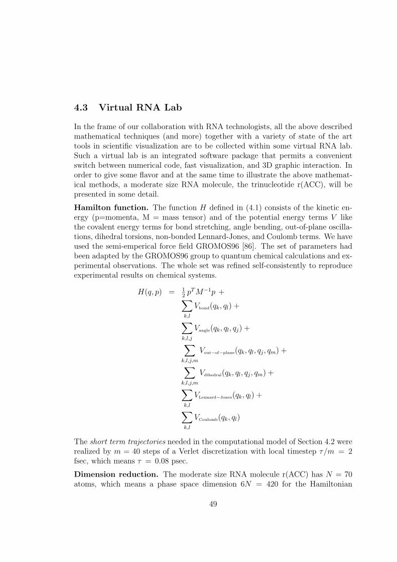
4.3 Virtual RNA Lab

In the frame of our collaboration with RNA technologists, all the above describedmathematical techniques (and more) together with a variety of state of the arttools in scientific visualization are to be collected within some virtual RNA lab.Such a virtual lab is an integrated software package that permits a convenientswitch between numerical code, fast visualization, and 3D graphic interaction. Inorder to give some flavor and at the same time to illustrate the above mathemat-ical methods, a moderate size RNA molecule, the trinucleotide r(ACC), will bepresented in some detail.

Hamilton function. The function H defined in (4.1) consists of the kinetic en-ergy (p=momenta, M = mass tensor) and of the potential energy terms V likethe covalent energy terms for bond stretching, angle bending, out-of-plane oscilla-tions, dihedral torsions, non-bonded Lennard-Jones, and Coulomb terms. We haveused the semi-emperical force field GROMOS96 [86]. The set of parameters hadbeen adapted by the GROMOS96 group to quantum chemical calculations and ex-perimental observations. The whole set was refined self-consistently to reproduceexperimental results on chemical systems.

H(q, p) = 12pT M−1p +∑

k,l

Vbond(qk, ql) +

∑k,l,j

Vangle(qk, ql, qj) +

∑k,l,j,m

Vout−of−plane(qk, ql, qj, qm) +

∑k,l,j,m

Vdihedral(qk, ql, qj, qm) +

∑k,l

VLennard−Jones(qk, ql) +

∑k,l

VCoulomb(qk, ql)

The short term trajectories needed in the computational model of Section 4.2 wererealized by m = 40 steps of a Verlet discretization with local timestep τ/m = 2fsec, which means τ = 0.08 psec.

Dimension reduction. The moderate size RNA molecule r(ACC) has N = 70atoms, which means a phase space dimension 6N = 420 for the Hamiltonian

49

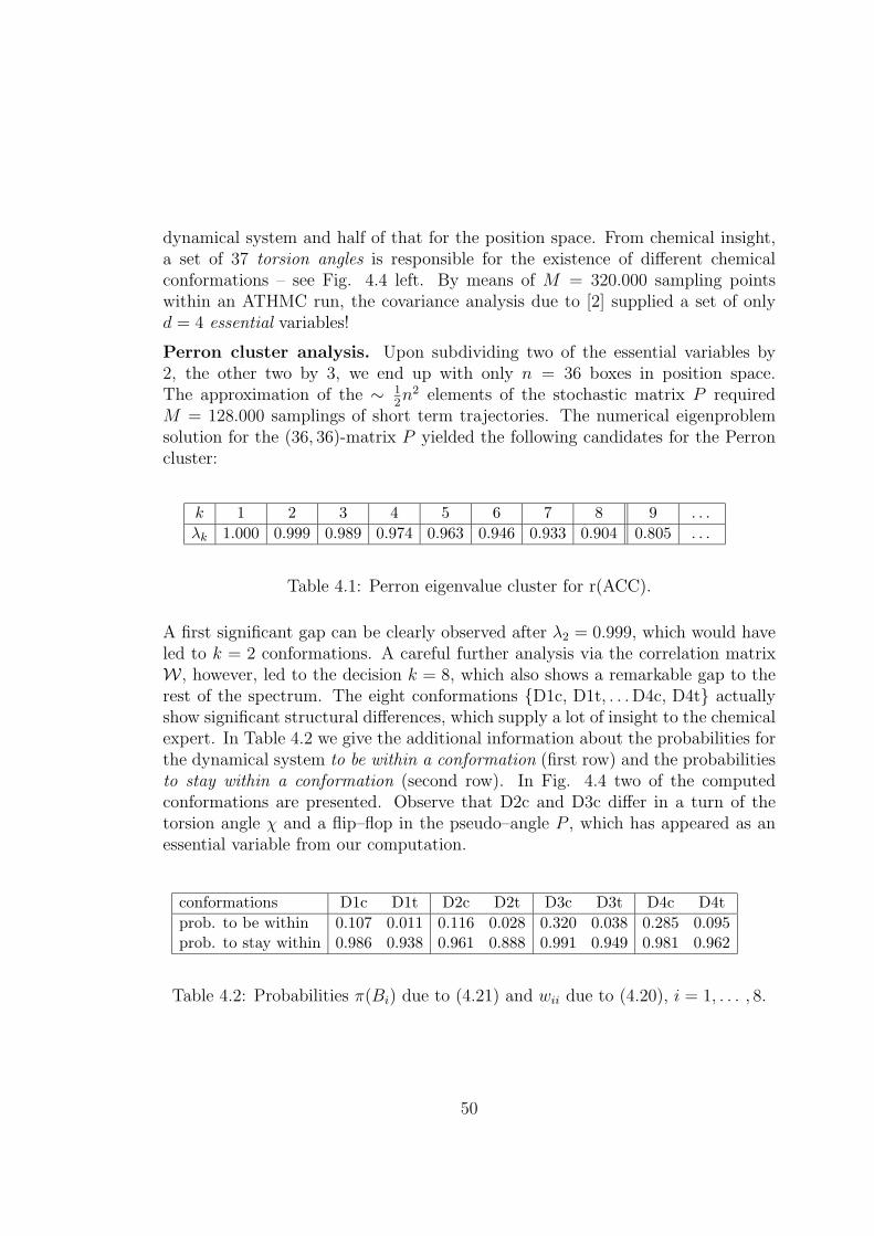
dynamical system and half of that for the position space. From chemical insight,a set of 37 torsion angles is responsible for the existence of different chemicalconformations – see Fig. 4.4 left. By means of M = 320.000 sampling pointswithin an ATHMC run, the covariance analysis due to [2] supplied a set of onlyd = 4 essential variables!

Perron cluster analysis. Upon subdividing two of the essential variables by2, the other two by 3, we end up with only n = 36 boxes in position space.The approximation of the ∼ 1

2n2 elements of the stochastic matrix P required

M = 128.000 samplings of short term trajectories. The numerical eigenproblemsolution for the (36, 36)-matrix P yielded the following candidates for the Perroncluster:

k 1 2 3 4 5 6 7 8 9 . . .

λk 1.000 0.999 0.989 0.974 0.963 0.946 0.933 0.904 0.805 . . .

Table 4.1: Perron eigenvalue cluster for r(ACC).

A first significant gap can be clearly observed after λ2 = 0.999, which would haveled to k = 2 conformations. A careful further analysis via the correlation matrixW , however, led to the decision k = 8, which also shows a remarkable gap to therest of the spectrum. The eight conformations {D1c, D1t, . . . D4c, D4t} actuallyshow significant structural differences, which supply a lot of insight to the chemicalexpert. In Table 4.2 we give the additional information about the probabilities forthe dynamical system to be within a conformation (first row) and the probabilitiesto stay within a conformation (second row). In Fig. 4.4 two of the computedconformations are presented. Observe that D2c and D3c differ in a turn of thetorsion angle χ and a flip–flop in the pseudo–angle P , which has appeared as anessential variable from our computation.

conformations D1c D1t D2c D2t D3c D3t D4c D4tprob. to be within 0.107 0.011 0.116 0.028 0.320 0.038 0.285 0.095prob. to stay within 0.986 0.938 0.961 0.888 0.991 0.949 0.981 0.962

Table 4.2: Probabilities π(Bi) due to (4.21) and wii due to (4.20), i = 1, . . . , 8.

50

εζαβ

γ

χP

Figure 4.4: Conformations D3c (left) and D2c (right) of the r(ACC) molecule. Left: 6 out of37 torsion angles. Look at the torsion angle χ and the pseudo-angle P to compare.

Conformational transition rates. The transition probabilities between the con-formations are collected in the (8, 8)-matrix W from (4.22) which here reads⎛⎜⎜⎜⎜⎜⎜⎜⎜⎜⎜⎝

0.986 5.310−3 1.410−5 8.110−3 5.310−4 0 0 05.110−2 0.938 1.010−2 4.610−6 2.610−4 6.310−4 0 1.110−74.010−5 3.110−3 0.949 4.810−2 0 3.610−7 3.610−5 2.610−52.710−3 1.610−7 5.710−3 0.991 7.710−8 0 8.010−4 1.210−94.910−4 2.510−5 0 2.110−7 0.961 1.310−2 2.510−2 7.310−4

0 2.610−4 5.010−7 0 5.610−2 0.888 3.510−3 5.210−20 0 4.710−6 9.010−4 1.010−2 3.410−4 0.981 7.410−30 1.410−8 1.010−5 4.010−9 9.010−4 1.510−2 2.210−2 0.962

⎞⎟⎟⎟⎟⎟⎟⎟⎟⎟⎟⎠

Recall that the diagonal elements of W are the same as the second row in Table 4.2,whereas the first row in Table 4.2 does not show up in W .

Extension to larger molecules. The above moderate size molecule is a quitegood candidate to sharpen the mathematician’s knife in this kind of collaboration.Biomolecules of real interest to our partners are larger – see e.g. the hammerheadmolecule as represented in Fig. 4.5.

This type of biomolecule consists of about 150 − 200 nucleotides; each nucleotidegives rise to roughly 12 torsion angles, which sums up to about 2.000 torsionangles that might generate conformations and should therefore be subdivided!Fortunately, chemists report that usually the larger the molecules, the stiffer theirstructure. If this is reliable, then covariance analysis for the associated HMCdata will bring up ”not too many” essential degrees of freedom that should still

51

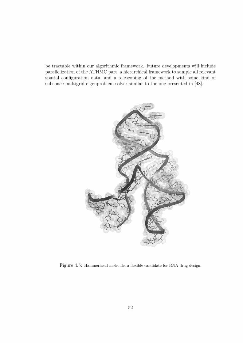
be tractable within our algorithmic framework. Future developments will includeparallelization of the ATHMC part, a hierarchical framework to sample all relevantspatial configuration data, and a telescoping of the method with some kind ofsubspace multigrid eigenproblem solver similar to the one presented in [48].

Figure 4.5: Hammerhead molecule, a flexible candidate for RNA drug design.

52

References

[1] M. P. Allen and D. J. Tildesley: Computer Simulations of Liquids. Clarendon,Oxford (1990).

[2] A. Amadei, A. Linssen, and H. Berendsen: Essential dynamics of proteins.Proteins, Vol. 17 (1993).

[3] V.I. Arnold: Mathematical Methods of Classical Mechanics. Second Edition.Springer (1989).

[4] I. Babuska, A. Miller: A feedback finite element method with a–posteriori errorestimation: part I. Comput. Meth. Appl. Mech. Engrg. 61 pp. 1–40 (1987).

[5] I. Babuska, W.C. Rheinboldt: Estimates for adaptive finite element compu-tations. SIAM J. Numer. Anal. 15 pp. 736–754 (1978).

[6] G. Bader, U. Nowak, P. Deuflhard: An advanced simulation package for largechemical reaction systems. In: R. Aiken (ed.), Stiff Computation, OxfordUniversity Press, pp. 255–264 (1985).

[7] A. Bachem, M. Junger, R. Schrader (eds.): Mathematik in der Praxis.Springer–Verlag (1995).

[8] R.E. Bank: PLTMG: A Software Package for Solving Elliptic Partial Differ-ential Equations. Users’ Guide 8.0 SIAM (1998).

[9] R.E. Bank, A.H. Sherman, A. Weiser: Refinement algorithms and data struc-tures for regular local mesh refinement. In: R. Stapleman et al (eds.), ScientificComputing, North–Holland, pp. 3–17 (1983).

[10] R.E. Bank, A. Weiser: Some a posteriori error estimates for elliptic partialdifferental equations. Math. Comp. 44, pp. 283–301 (1985).

[11] P. Bastian, K. Birken, K. Johannsen, S. Lang, N. Neuss, H. Rentz-Reichert,C. Wieners: UG – A flexible software toolbox for solving partial differentialequations. Computing and Visualization in Science, Vol. 1, pp. 27–40 (1997).

[12] P. Bastian, G. Wittum: Adaptive multigrid methods: The UG concept. In: W.Hackbusch and G. Wittum (eds.), Adaptive Methods – Algorithms, Theoryand Applications, Series Notes on Numerical Fluid Mechanics, Vol. 46, pp. 17–37, Vieweg, Braunschweig (1994).

53

[13] R. Beck, P. Deuflhard, R. Hiptmair, B. Wohlmuth, R.H.W. Hoppe: AdaptiveMultilevel Methods for Edge Element Discretizations of Maxwell’s Equations.Surveys of Mathematics for Industry, accepted for publication (1999).

[14] R. Beck, B. Erdmann, R. Roitzsch: KASKADE 3.0 – User’s Guide.ftp://ftp.zib.de/pub/kaskade (1996).

[15] J. Bey: Tetrahedral Grid Refinement. Computing, Vol. 55, No. 4, pp. 355–378(1995).

[16] F.A. Bornemann, B. Erdmann, R. Kornhuber: Adaptive multilevel methods inthree space dimensions. Int. J. Num. Meth. in Eng. 36, pp. 3187–3203 (1993).

[17] F.A. Bornemann, B. Erdmann, R. Kornhuber: A posteriori error estimatesfor elliptic problems in two and three space dimensions. SIAM J. Numer. Anal.33, pp. 1188–1204 (1996).

[18] F. Bornemann: An adaptive multilevel approach to parabolic equations I. Gen-eral theory and implementation. IMPACT Comput. Sci. Engrg. 2, pp. 279–317(1990).

[19] F. Bornemann: An adaptive multilevel approach to parabolic equations II.Variable–order time discretization based on a multilevel error correction. IM-PACT Comput. Sci. Engrg. 3, pp. 93–122 (1991).

[20] F. Bornemann, P. Deuflhard: The Cascadic Multigrid Method for EllipticProblems. Numer. Math. 75, Springer International, pp. 135–152 (1996).

[21] A. Bossavit: Solving Maxwell’s equations in a closed cavity and the questionof spurious modes. IEEE Trans. Mag., 26(2), pp. 702–705 (1990).

[22] R. Bradel, A. Kleinke, K.-H. Reichert: Molar Mass Distribution of Micro-bial Poly (D-3-Hydroxybutyrate) in the Course of Intracellular Synthesis andDegradation. Makromol. Chem., Rapid Commun. 12, p. 583 (1991).

[23] D. Braess, W. Hackbusch: A new convergence proof for the multigrid methodincluding the V-cycle. SIAM. J. Numer. Anal., 20, pp. 967–975 (1983).

[24] J. Bramble, J. Pasciak, J. Xu: Parallel multilevel preconditioners.Math. Comp. 55, pp. 1–22 (1990).

[25] J. Bramble, J. Pasciak, J. Wang, J. Xu: Convergence estimates for multigridalgorithms without regularity assumptions. Math. Comp. 57, pp. 23–45 (1991).

54

[26] A. Brandt: Multi–level adaptive solutions to boundary–value problems.Math. Comp. 31, pp. 333–390 (1977).

[27] M.–O. Bristeau, G. Etgen, W. Fitzigibbon, J.–L. Lion, J. Periaux, M. Wheeler(eds.): Computational Science for the 21st Century. Tours, France. Wiley–Interscience–Europe (1997).

[28] M. Dellnitz, A. Hohmann: A subdivision algorithm for the computation of un-stable manifolds and global attractors. Numer. Math. 75, pp. 293–317 (1997).

[29] M. Dellnitz, O. Junge: On the approximation of complicated dynamical be-havior. SIAM J. Num. Anal. 36(2), pp. 491–515 (1999).

[30] P. Deuflhard: Cascadic Conjugate Gradient Methods for Elliptic Partial Dif-ferential Equations. Algorithm and Numerical Results. In [61], pp. 29–42(1994).

[31] P. Deuflhard: Uniqueness Theorems for Stiff ODE Initial Value Problems. In:D.F. Griffiths and G.A. Watson (eds.): Numerical Analysis 1989, LongmanScientific & Technical, Harlow, Essex, UK, pp. 74–205 (1990).

[32] P. Deuflhard and F. Bornemann: Numerische Mathematik II — Integrationgewohnlicher Differentialgleichungen. Walter de Gruyter, Berlin, New York(1994).

[33] P. Deuflhard, M. Dellnitz, O. Junge, Ch. Schutte: Computation of EssentialMolecular Dynamics by Subdivision Techniques. In [36], pp. 98–115 (1998).

[34] P. Deuflhard, T. Friese, F. Schmidt, R. Marz, H.–P. Nolting: Effiziente Eigen-modenberechnung fur den Entwurf integriert–optischer Chips. In [56], pp. 267–279 (1996).

[35] P. Deuflhard, J. Hohmann: Numerical analysis. A First Course in ScientificComputation. Berlin, New York: de Gruyter (1995).

[36] P. Deuflhard, A. Hermans, B. Leimkuhler, A.E. Mark, S. Reich, andR.D. Skeel (eds.): Computational Molecular Dynamics: Challenges, Meth-ods, Ideas. Lecture Notes in Computational Science and Engineering, Vol. 4,Springer-Verlag (1998).

[37] P. Deuflhard, W. Huisinga, A. Fischer, and Ch. Schutte: Identification ofalmost invariant aggregates in reversible nearly uncoupled Markov chains. Lin.Alg. Appl., accepted.

55

[38] P. Deuflhard, J. Lang, U. Nowak: Recent Progress in Dynamical Process Si-mulation. In: H. Neunzert (ed.): Topics in Industrial Mathematics, Wiley &Teubner Publishers, pp. 122–137 (1996).

[39] P. Deuflhard, P. Leinen, H. Yserentant: Concepts of an Adaptive HierarchicalFinite Element Code. IMPACT Comp. Sci. Eng. 1, pp. 3–35 (1989).

[40] P. Deuflhard, M. Seebass: Adaptive Multilevel FEM as Decisive Tools in theClinical Cancer Therapy Hyperthermia. In: Choi–Hong Lai, Peter Bjørstad,Mark Cross, O. Widlund (eds.), Procs. 11th International Conference on Do-main Decomposition Methods (DD11), UK, 1998 (to appear 1999).

[41] P. Deuflhard, M. Seebass, D. Stalling, R. Beck, H.C. Hege: HyperthermiaTreatment Planning in Clinical Cancer Therapy: Modelling, Simulation, andVisualization. Plenary Keynote talk, 15th IMACS World Congress 1997. In:Achim Sydow (ed.), Vol. 3, Computational Physics, Chemistry and Biology.Wissenschaft and Technik Verlag, pp. 9–17 (1997).

[42] P. Deuflhard, M. Weiser: Local Inexact Newton Multilevel FEM for NonlinearElliptic Problems. In [27], pp. 129–138 (1997).

[43] P. Deuflhard, M. Weiser, M. Seebass: A New Nonlinear Elliptic MultilevelFEM Appied to Regional Hyperthermia. Konrad Zuse Zentrum, Preprint SC98-35 (1998).

[44] P. Deuflhard, M. Weiser: Global Inexact Newton Multilevel FEM for NonlinearElliptic Problems. In [53], pp. 71–89 (1998).

[45] P. Deuflhard, M. Wulkow: Computational Treatment of Polyreaction Kineticsby Orthogonal Polynomials of a Discrete Variable. IMPACT Comp. Sci. Eng.1,pp. 269–301 (1989).

[46] P. Deuflhard, M. Wulkow: Simulationsverfahren fur die Polymerchemie. In[7], pp. 117–136 (1995).

[47] A. Fischer, F. Cordes, and Ch. Schutte: Hybrid Monte Carlo with adaptivetemperature in mixed canonical ensemble: Efficient conformational analysisof RNA. J. Comput. Chem., 19(15), pp. 1689-1697 (1998).

[48] T. Friese, P. Deuflhard, F. Schmidt: A Multigrid Method for the ComplexHelmholtz Eigenvalue Problem. In: Procs. 11th International Conference onDomain Decomposition Methods (DD11), UK, 1998 (to appear 1999).

56

[49] H. Gajewski, K. Zacharias: On an Initial Value Problem for a CoagulationEquation with Growth Term. Math. Nachr. 109, pp. 135–156 (1982).

[50] G.H. Golub, C.F. Van Loan: Matrix Computations. The Johns Hopkins Uni-versity Press, Baltimore, London, 2nd Edition (1989).

[51] H. Grubmuller, P. Tavan. Molecular dynamics of conformational substates fora simplified protein model. J. Chem. Phys. 101 (1994).

[52] W. Hackbusch: Multi–Grid Methods and Applications. Springer Verlag,Berlin, Heidelberg, New York (1995).

[53] W. Hackbusch, G. Wittum (eds.): Multigrid Methods, Lecture Notes in Com-putational Science and Engineering. Vol. 3, Springer–Verlag (1998).

[54] H.-C. Hege, M. Seebaß, D. Stalling, M. Zockler: A Generalized MarchingCubes Algorithm Based On Non-Binary Classifications. ZIB Preprint SC 97–05 (1997).

[55] R. Hiptmair: Multilevel Preconditioning for Mixed Problems in Three Dimen-sions. Ph.D. Thesis, Wissner, Augsburg (1996).

[56] K.–H. Hoffmann, W. Jager, T. Lohmann, H. Schunk (eds.): MATHEMATIKSchlusseltechnologie fur die Zukunft. Springer (1997).

[57] C.S. Hsu: Cell–to–Cell Mapping. A Method of Global Analysis for NonlinearSystems. In: F. John, J.E. Marsden, L. Sirovich (eds.): Applied MathematicalSciences, Vol. 64, Springer–Verlag.

[58] W. Huisinga, Ch. Best, R. Roitzsch, Ch. Schutte, and F. Cordes: From Sim-ulation Data to Conformational Ensembles: Structure and Dynamics BasedMethods. Konrad-Zuse-Zentrum Berlin. Preprint SC 98–36 (1998).

[59] P. Iedema, M. Wulkow, H. Hoefsloot: Modeling Molecular Weight and De-gree of Branching Distribution of Low Density Polyethylene. Submitted toMacromolecules (1999).

[60] V.E. Katsnelson: Conditions under which systems of eigenvectors of someclasses of operators form a basis. Funkt Anal. Appl.1, pp. 122–132 (1967).

[61] D.E. Keyes, J. Xu (eds.): Domain Decomposition Methods in Scientific andEngineering Computing. AMS Series Contemporary Mathematics, Vol. 180,Providence (1994).

57

[62] R. Kornhuber, R. Roitzsch: On adaptive grid refinement in the presence of in-ternal or boundary layers. IMPACT Comput. Sci. Engrg. 2, pp. 40–72 (1990).

[63] J. Lang: Adaptive FEM for Reaction–Diffusion Equations. Appl. Numer.Math. 26, pp. 105–116 (1998).

[64] J. Lang: Adaptive Multilevel Solution of Nonlinear Parabolic PDE Systems.Theory, Algorithm, and Applications. Habilitation Thesis, Free University ofBerlin, 1999. Konrad–Zuse-Zentrum Berlin, Preprint SC 99–20 (1999).

[65] J. Lang, B. Erdmann, M. Seebass: Impact of Nonlinear Heat Transfer onTemperature Distribution in Regional Hyperthermia. Accepted for publicationin IEEE Transaction on Biomedical Engineering (1999).

[66] W. E. Lorensen, H. E. Cline: Marching Cubes: A high resolution 3D surfaceconstruction algorithm. Computer Graphics 21:4, pp. 163-169 (1987).

[67] J. Mandel, S.F. McCormick: A multilevel variational method for Au = ΛBuon composite grids. J. Comp. Phys. 80, pp. 442-452 (1989).

[68] B. Mayfield: Nonlocal Boundary Conditions for the Schrodinger Equation.PhD thesis, University of Rhode Island, Providence, RI, (1989).

[69] A.H.E. Muller, D. Yan, M. Wulkow: Molecular Parameters of HyperbranchedPolymers Made by Self–condensing Vinyl Polymerization. I. Molecular weightdistribution. Macromolecules 30, pp. 7015 (19997).

[70] J.C. Nedelec: Mixed finite elements in R3. Numer. Math. 35, pp. 315–341(1980).

[71] M.E. Go Ong: Hierarchical Basis Preconditioners for Second Order EllipticProblems in Three Ddimensions. PhD Thesis, University of California, LosAngeles (1989).

[72] H.H. Pennes: Analysis of tissue and arterial blood temperatures in the restinghuman forearm. J. Appl. Phys. 1, pp. 93-122 (1948).

[73] M.C. Rivara: Algorithms for refining triangular grids suitable for adaptiveand multigrid techniques. Int. J. Numer. Meth. Engrg. 20, pp. 745-756 (1984).

[74] Y. Saad: Numerical Methods for Large Eigenvalue Problems. Manchester Uni-versity Press (1992).

58

[75] J.M. Sanz-Serna, M.P. Calvo: Numerical Hamiltonian Problems. Chapman &Hall (1994).

[76] F. Schmidt: An adaptive approach to the numerical solution of Fresnel’s waveequation. IEE Journal of Lightwave Technology, 11(9), pp. 1425–1435 (1993).

[77] F. Schmidt: Computation of discrete transparent boundary conditions forthe 2D Helmholtz equation. Konrad–Zuse–Zentrum Berlin. Preprint SC 97-64 (1997).

[78] F. Schmidt, P. Deuflhard: Discrete Transparent Boundary Conditions for theNumerical Solution of Fresnel’s equation. Computers Math. Applic. 29, No.9, pp. 53–76 (1995).

[79] F. Schmidt, D. Yevick: Discrete transparent boundary conditions forSchrodinger–type equations. J. Comput. Phys., Vol. 134, pp. 96–107 (1997).

[80] Ch. Schutte: Conformational Dynamics: Modelling, Theory, Algorithm,and Application to Biomolecules. Habilitation Thesis. Konrad–Zuse–ZentrumBerlin, Preprint SC 99–18 (1999).

[81] Ch. Schutte, A. Fischer, W. Huisinga, and P. Deuflhard: A Direct Approachto Conformational Dynamics based on Hybrid Monte Carlo. J. Comput. Phys.151, Special Issue on Computational Molecular Biophysics, pp. 146–168(1999).

[82] V.V. Shaidurov: Some estimates of the rate of convergence for the cas-cadic conjugate–gradient method. Preprint, Otto–von–Guericke–Universitat.Magdeburg (1994).

[83] M. Seebass, D. Stalling, M. Zockler, H.-C. Hege, P. Wust, R. Felix, P. Deu-flhard: Surface Mesh Generation for Numerical Simulations of HyperthermiaTreatments. In: Procs. 16th Annual Meeting of the European Society for Hy-perthermic Oncology, p. 146, Berlin (1997).

[84] M. Seebass, D. Stalling, J. Nadobny, P. Wust, R. Felix, P. Deuflhard: Three-Dimensional Finite Element Mesh Generation for Numerical Simulations ofHyperthermia Treatments, Proc. 7th Int. Congress on Hyperthermic Oncology,Rome, Vol. 2, pp. 547-548 (1996).

[85] C.W. Song, A. Lokshina, J.G. Rhee, M. Patten, and S.H. Levitt: Implica-tion of blood flow in hyperthermic treatment of tumors. IEEE Trans. Biomed.Engrg. 31, pp. 9-16 (1984).

59

[86] W.F. van Gunsteren, S.R. Billeter, A.A. Eising, P.H. Hunenberger, P. Kruger,A.E. Mark, W.R.P. Scott, and I.G. Tironi: Biomolecular Simulation: TheGROMOS96 Manual and User Guide. vdf Hochschulverlag AG, ETH Zurich(1996).

[87] M. Wulkow: Numerical Treatment of Countable Systems of Ordinary Differen-tial Equations. Dissertation, Konrad–Zuse–Zentrum Berlin. Technical ReportTR 90–08 (1990).

[88] M. Wulkow: Feature article – The Simulation of Molecular Weight Distri-butions in Polyreaction Kinetics by Discrete Galerkin Methods. Macromol.Theory Simul. 5, pp. 393–416 (1996).

[89] J. Xu: Theory of Multilevel Methods. PhD Thesis, Report No. AM 48, De-partment of Mathematics, Pennsylvania State University (1989).

[90] J. Xu: Iterative methods by space decomposition and subspace correction.SIAM Review 34 pp. 581–613 (1992).

[91] H. Yserentant: On the multilevel splitting of finite element spaces. Nu-mer. Math. 58 pp. 163–184 (1986).

60