Differential equations and solution of linear systemsmath.univ-lille1.fr/~chehab/Rech/chehablaminie.pdf · 2007-04-06 · J.-P. Chehab, J. Laminie / Differential equations and solution

Numerical Algorithms (2005) 40: 103–124DOI 10.1007/s11075-005-1523-5 Springer 2005

Differential equations and solution of linear systems

Jean-Paul Chehab a,b and Jacques Laminie b

a Laboratoire de Mathématiques Paul Painlevé, CNRS UMR 8524, Université de Lille, FranceE-mail: [email protected]

b Laboratoire de Mathématiques, CNRS UMR 8628, Equipe ANEDP, Université Paris Sud, Orsay, FranceE-mail: [email protected]

Received 14 June 2003; accepted 12 December 2004Communicated by H. Sadok

Many iterative processes can be interpreted as discrete dynamical systems and, in cer-tain cases, they correspond to a time discretization of differential systems. In this paper, wepropose to derive iterative schemes for solving linear systems of equations by modeling theproblem to solve as a stable state of a proper differential system; the solution of the originallinear problem is then computed numerically by applying a time marching scheme. We dis-cuss some aspects of this approach, which allows to recover some known methods but also tointroduce new ones. We give convergence results and numerical illustrations.

Keywords: differential equation, numerical schemes, numerical linear algebra,preconditioning

AMS subject classification: 65F10, 65F35, 65L05, 65L12, 65L20, 65N06

1. Introduction

The connections between differential equations and linear algebra are numerous:one the one hand, linear algebra tools and concepts are used for studying theoretical as-pects of ODEs, e.g., such as the properties of equilibrium points [14,15,19]; in a parallelway, techniques of linear numerical algebra are intensively applied in numerical analysisof ODEs for the analysis of time marching methods. On the other hand, in some cases,iterative processes for solving linear as well as nonlinear systems of equations can bederived from the discretization of a ODE, as, e.g., pointed out in [8,9,11,15,19] for thesolution fixed points, but also in [7] for the interpretation of convergence accelerationalgorithms.

During the last two decades, Numerical Linear Algebra (NLA) has been consid-erably enriched with the introduction of methods like GMRES [18], Bi-Cgstab [20] orQMR [12] since they allow the efficient solution of large scale non-symmetric prob-lems. These algorithms are based on Krylov subspace techniques and, if we omit somevariations on these methods, no new algorithm was proposed since, making the precon-ditioning a central topic in NLA [3].

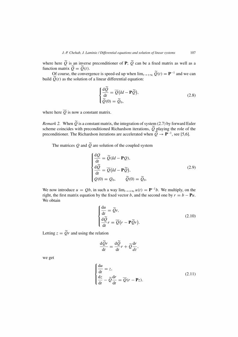
104 J.-P. Chehab, J. Laminie / Differential equations and solution of linear systems

Several classical iterative methods can be recovered by a proper discretization ofODEs, particularly some decent methods can be interpreted as discrete versions of gradi-ent flows [13]. One of the simplest example is given by the relation between Richardson-like methods and forward Euler’s schemes, the relaxation parameter and the time step-size playing the same role, see [9,17]. Let P be a n × n symmetric positive definitematrix. Consider the equation

dU

dt= b − PU,

U(0) = U0,

(1.1)

whose the steady state is the solution of the linear system

PU = b. (1.2)

The steady state is asymptotically stable and can be then computed numerically by usingan explicit time marching scheme. This is a simple but very important property since,in that case, the time discretization consists in building a sequence of vector satisfying asimple (linear) recurrence relation. The application of the Forward Euler scheme to (1.1)generates the iterations

Uk+1 = Uk + �t(b − PUk

), k = 0, . . . . (1.3)

(1.3) is nothing else but the classical Richardson scheme; if P is positive definite, thestability condition is 0 < �t < 2/ρ(P), where ρ(P) denotes the spectral radius of P.However, since the goal is to approach the steady state as fast as possible, many variants,not directly connected to numerical analysis of ODEs can be considered; the time step �t

can depend on k so some descent methods enter in this framework. Of course otherclassical methods can be recovered following this approach.

In this article we propose to generate numerical methods in NLA by modeling thelinear system to be solved as a given state of a dynamical system; the solution can bereached asymptotically, as a (asymptotically stable) steady state, but also at finite time(shooting methods). In that way, any (stable) numerical scheme for the integration ofsuch a problem can be presented as a method for solving linear systems. This idea wasintroduced in [10] for building sequences of inverse preconditioners. We then proposeto generate schemes in numerical linear algebra following the two steps:

1. Construction/derivation of a dynamical system.

2. Discretization of the dynamical system by, e.g., time marching techniques.

We here discuss of some ideas of this approach and show that the derived methodscan be of numerical interest.

The article is organized as follows: in section 2 we consider a family of coupleddynamical system whose the discretization allows to recover classical descent methodbut also to defined new schemes. Then, in section 3, we propose to reach numerically the

J.-P. Chehab, J. Laminie / Differential equations and solution of linear systems 105

solution at finite time of the linear system by implementing a shooting method. In sec-tion 4, we consider different time marching schemes for the differential systems as (1.1).Finally, we present some numerical results in section 5.

The numerical results we present were obtained by using Matlab © 6 software ona cluster of Bi-processor 800 (Pentium III) at Université Paris XI, Orsay, France.

2. Coupled differential systems and descent methods

Basically, the iterations of a descent method verify a recurrence relation of type

uk+1 = uk + αkzk, (2.1)

where uk is the approximation of the solution of the system at step k, αk is the step-sizeand zk the descent direction vector. The residual rk = b − Puk satisfies the relation

rk+1 = rk − αkPzk. (2.2)

Here P is a regular matrix, not necessarily symmetric positive definite. If αk plays therole of a time step, we can identify the above iterative process to a time marching schemeapplied to a differential system. One way to recover the above stencil is to consider thetime discretization of linear differential systems, such as

du

dt

dz

dt

=

(A B

C D

)(r

z

)

. (2.3)

We have set here r = b − Pu. So, up to suitable assumptions on the matrices A, B,C and D, the convergence of the system to the trivial equilibrium point (r, z) = (0, 0)

implies that limt→+∞ u(t) = P−1b. We hereafter discuss on different strategies forchoosing these matrices.

2.1. The general case

The system (2.3) is consistent with the solution of the linear problem Pu = b oncethe matrix

(A B

C D

)

is regular. Let us neglect the time derivative in z, the above system reads

du

dt0

=(

A B

C D

)(r

z

)

. (2.4)


If we eliminate z with the algebraic relation Cr + Dz = 0, we obtain formally

du

dt= (

A − BD−1C)r,

say

dr

dt= −P

(A − BD−1C

)r.

Hence, if(A − BD−1C

) = P−1, (2.5)

the solution of the linear system is reached in one iteration by taking �t = 1: S =A−BD−1C is a Schur complement which can be interpreted as an inverse preconditionerof P. This indicates how to choose the matrices A, B, C, D. For example, if we letA = 0, B = −C = Id, then, according to (2.5), the matrix D must be chosen such asPD−1 ≈ Id, that means that D must be a preconditioner of P.

In a general way, the iterative solution of the algebraic equation Cr + Dz = 0can be seen as a projection on a linear manifold. If we take D = P, the projectionreduces to the equation r = Pz and can be interpreted as a preconditioning step; theimplementation of the preconditioning consisting in solving this last system iteratively,see also section 5.

Remark 1. In (2.4), the expression Bz together with the relation z = −D−1Cu can beinterpreted as a feedback control of the system, see also [4] for the relations betweencontrol of linear systems and descent methods.

2.2. A family of descent methods

2.2.1. Derivation of the systemIn order to build inverse preconditioners of a given regular matrix P, it was pro-

posed in [10] to integrate numerically matrix differential equations which have P−1 assteady state, such as the following Riccati equation:

dQ

dt= Q(Id − PQ),

Q(0) = Q0.

(2.6)

It can be shown, under suitable assumptions, that Q(t) converges to P−1 as t → +∞,see [10]. Unfortunately, since the equation is nonlinear, it is not possible to derive asimple (linear) recurrence relation when integrating this system by, e.g., Euler’s method.For these reasons, we consider a linearized version of the above system:

dQ

dt= Q̃(Id − PQ),

u(0) = u0,

(2.7)


where here Q̃ is an inverse preconditioner of P; Q̃ can be a fixed matrix as well as afunction matrix Q̃ = Q̃(t).

Of course, the convergence is speed-ed up when limt→+∞ Q̃(t) = P−1 and we canbuild Q̃(t) as the solution of a linear differential equation:

dQ̃

dt= Q

(Id − PQ̃

),

Q̃(0) = Q̃0,

(2.8)

where here Q is now a constant matrix.

Remark 2. When Q̃ is a constant matrix, the integration of system (2.7) by forward Eulerscheme coincides with preconditioned Richardson iterations, Q̃ playing the role of thepreconditioner. The Richardson iterations are accelerated when Q̃ → P−1, see [5,6].

The matrices Q and Q̃ are solution of the coupled system

dQ

dt= Q̃(Id − PQ),

dQ̃

dt= Q

(Id − PQ̃

),

Q(0) = Q0, Q̃(0) = Q̃0.

(2.9)

We now introduce u = Qb, in such a way limt→+∞ u(t) = P−1b. We multiply, on theright, the first matrix equation by the fixed vector b, and the second one by r = b − Pu.We obtain

du

dt= Q̃r,

dQ̃

dtr = Q

(r − PQ̃r

).

(2.10)

Letting z = Q̃r and using the relation

dQ̃r

dt= dQ̃

dtr + Q̃

dr

dt,

we get

du

dt= z,

dz

dt− Q̃

dr

dt= Q(r − Pz).

(2.11)


Finally, since dr/dt = −Pz we obtain the system

du

dt= z,

dz

dt= −Q̃Pz + Q(r − Pz).

(2.12)

Remark 3. Following the presentation of (2.3), this last systems writes as

du

dt

dz

dt

=

(0 I

Q −(Q̃ + Q

)P

)(r

z

)

. (2.13)

The associate Schur’s complement is here S = −P−1(Q̃ + Q)−1Q.

Remark 4. We can of course repeat the process by defining Q as the solution of a lin-ear differential equation, and so on. More precisely, if we consider N levels of theseiterations, we obtain the differential system

du

dt= z1,

for i = 1, . . . , N − 1,dzi

dt= (Qi + Qi+1)Pzi + zi+1

QN = Id, zN = 0

(2.14)

where the matrices Qi are defined by

dQi

dt= Qi+1(Id − PQi),

and where we have set zi = Qir , i = 1, . . . , N − 1.

2.2.2. Some derived differential systemsIn (2.12), the matrix Q̃ must be computed at each step for integrating the system:

this is not compatible with the general stencil of a descent method in which only se-quences of vector and fixed matrices are handled. A way to overcome this difficulty isto approach the matrix Q̃P. We hereafter propose some dynamical systems deduced bysuch approximations and that allow to derive descent methods by numerical integration.

1. Q̃P ≈ Id. This approximation is motivated by the assumption limt→+∞ Q̃ = P−1.The dynamical system is, in that case,

du

dt= z,

dz

dt= −z + Q(r − Pz).

(2.15)


2. Q̃ ≈ Q. The derived dynamical system is then

du

dt= z,

dz

dt= Q(r − 2Pz).

(2.16)

3. Q̃P = 0. This approximation is obtained by considering the steady state z = 0. Thedynamical system is here

du

dt= z,

dz

dt= Q(r − Pz).

(2.17)

4. Replace dz/dt by 0 in (2.12)

du

dt= z,

Q̃Pz = Q(r − Pz).

(2.18)

Various dynamical systems can be derived by considering different approximationsof Q̃P. Let us consider the particular case Q̃P ≈ Id, QP ≈ α(t)Id. The discretizationof such a system by a forward Euler method with variable time step reads

{uk+1 = uk + βkzk,

zk+1 = rk + αkzk.(2.19)

This is the general stencil of the conjugate gradient method.

2.2.3. Convergence resultsAs stated before, any (stable) discretization of the dynamical systems reads as a

numerical method for solving Pu∗ = b. Of course, these methods must be explicit andtheir stability require the equilibrium point (u, z) = (u∗, 0) or (r, z) = (0, 0) to beasymptotically stable. The differential systems can be written as

du

dt

εdz

dt

= M

(r

z

)

,

with ε = 0 or 1. Here M is the matrix of the system. The point (r, z) = (0, 0)

is asymptotically stable when all the eigenvalues of M are of real part bounded frombelow by a strictly negative real number, see [14].


We have the following result:

Proposition 5. We set Q = Id. Then, the vector u defined the differential system (2.15)converges to P−1b as t → +∞. Moreover (r − Pz) → 0, at an exponential rate, ast → +∞.

Proof. System (2.15) is equivalent to

dr

dt

dz

dt

=

(0 −PId −Id − P

)(r

z

)

. (2.20)

We establish the result by showing that the real part of the eigenvalues of the matrix

M =(

0 P−Id Id + P

)

are positive: in that case all the orbits converge to the equilibrium point at an exponentialrate [14]. Let (u, v)T be an eigenvector of M with associate eigenvalue λ. We have therelations

Pv = λu, −u + (Id + P)v = λv,

from which we deduce

(1 − λ)Pu = λ(1 − λ)u.

Hence, the eigenvalues of M are {1, σ (P)}, where σ(P) is the spectrum of P.Now, returning to (2.15) and taking the addition of the two equations, we obtain,

after multiplication by −P and after the usual simplifications:

dr − Pz

dt+ P(r − Pz) = 0.

We integrate this equation and we get

(r − Pz)(t) = e−tP(r − Pz)(0).

Hence the last assertion. The proof is achieved. �

In a similar way, we can prove the following results:

Proposition 6. We set Q = Id. Assume that the eigenvalues of P are real and largerthan 1. Then, the vector u defined the differential system (2.16) converges to P−1b ast → +∞.

Proof. We proceed as above. Let w = (u, v)t be an eigenvector of M with λ as associ-ated eigenvalue. We have the relation

(1 − 2λ)Pu = λ2u.


It follows that λ2/(1 − 2λ) is an eigenvalue of P (we can not have λ = 12 because in that

case w = 0 and w is a eigenvector). So λ verify the equations

λ2 − 2µλ + µ = 0,

for µ ∈ σ(P). We have then

λ = µ ±√

µ2 − µ

Hence, since µ > 1, we have λ > 0. �

The stability of fixed points of system (2.17) is given by:

Proposition 7. We let Q = Id. Assume that all the eigenvalues of P are real and largerthan 1

2 . Then, the vector u defined the differential system (2.17) converges to P−1b ast → +∞.

Proof. The proof is very similar to the previous one. �

Remark 8. Assumptions like σ(P) ⊂ [ 12 , +∞[ are not restrictive at all: indeed, they can

be obtained after a simple rescaling since P is positive definite.

Iterations (2.19) can be derived by time discretization of the system

du

dt= z,

z = r − α(t)z.

(2.21)

Here α(t) is a (regular) function to be chosen. Now, using the relation

dr

dt= −P

du

dt,

we have

dz

dt= −Pz − α(t)

dz

dt− dα(t)

dtz.

Hence,

dz

dt= − 1

1 + α(t)

(

Pz + dα(t)

dtz

)

,

and therefore

d2r

dt2= − 1

1 + α(t)

(

P + dα(t)

dtId

)dr

dt.


From these equations, we deduce the following result:

Proposition 9. Assume that

(i) α(t) > −1, ∀t � 0,

(ii) dα(t)/dt > λmin(P).

Then all the orbits of (2.18) converge to the solution (0, 0).

Proof. The proof is obtained by a classical computation. �

Remark 10. All the coupled dynamical systems introduced above can be written as asecond order differential system. Indeed, thanks to the relation du/dt = z, we canwrite (2.12) as

d2u

dt2+ (

Q̃ + Q)P

du

dt+ QPu − Qb = 0. (2.22)

Remark 11. Bi-gradient methods can be obtained by a particular time discretization ofa coupled dynamical system. In this case there are two descent direction vectors.

For example, Bi-Cgstab is derived from

dr

dt= −P(s + q),

q = r + ω0(Id − αP)q,

s = r − ωPq.

(2.23)

Here, s and q are the descent direction vectors [20].

3. Shooting methods

The solution of the linear problem Pu = b was previously defined as the steadystate of some differential systems. A way to reach the solution for a finite value of theindependent variable is to model the linear system as an objective. Let us turn back tothe stencil of the differential systems associated to the descent methods, as they werebuilt above. We have the system

dr

dt

dz

dt

=

(0 −PC D

)(r

z

)

. (3.1)

Now, let T > 0 be a given real number. We define the problem as follows:

Find z(0) ∈ Rn such that r(T ) = 0. (S)


Letting

M =(

0 −PC D

)

,

we rewrite problem (S) as

Given r(0), find z(0), such that(

0z(T )

)

= e−TM(

r(0)

z(0)

)

.(3.2)

At this point we introduce the flow function F defined by

F : z(0) �−→ r(T ),

in such a way S reduces to find a zero of F . We now consider the case C = Id,D = −Id − P.

Remark 12. A natural idea could be to consider a pointwize version of the classicalshooting method for solving second order boundary problem. This consists in solvingtwice the problem

dr

dt= −Pz,

dz

dt= −z + (r − Pz),

r(0) = r0, z(0) = z0

(3.3)

for two different values of z(0). Denoting by r1(t) and r2(t) (resp. z1(t) and z2(t)) thesolutions of the above system for z(0) = ξ1 and z(0) = ξ2, we build the function r(t) asr(t) = 1r1(t) + 2r2(t) where 1 and 2 are two diagonal matrices such that

r(0) = 1r1(t) + 2r2(0) and 0 (= r(T )) = 1r1(T ) + 2r2(T ).

We have immediately 2 = Id − 1 and

(1)i = (r2(T ))i

(r2(T ))i − (r1(T ))i

.

Unfortunately, this not allows to give a simple and explicit value of z(t) with F(z(0))

= 0 since we have

z(t) = P−11Pz1(t) + P−12Pz2(t).


4. Numerical integration

4.1. Enhanced stable time marching scheme

4.1.1. Definition of the schemeThe computation of a steady state by an explicit scheme can be speed-ed up by

enhancing the stability domain of the scheme since it allows to use larger time steps; inthat context the accuracy of a time marching scheme is not a priority. A simple way toderive more stable methods is to use the parametrized one step schemes and to fit theparameters, not for increasing the accuracy such as in the classical schemes (Heun’s,Runge–Kutta’s), but for improving the stability.

For example, in [9] it was defined a method for computing iteratively fixed pointswith larger descent parameter starting from a specific numerical time scheme. Moreprecisely, this method consists in integrating the differential equation

dU

dt= F(U),

U(0) = U0,

(4.1)

by the two steps scheme

K1 = F(Uk),

K2 = F(Uk + �tK1),

Uk+1 = Uk + �t(αK1 + (1 − α)K2

).

(4.2)

Here α is a parameter to be fixed. This scheme allows a larger stability as compared tothe Forward Euler scheme. For example, when F(U) = b − PU , we have the result:

Lemma 13. Assume that P is positive definite, then the scheme is convergent iff

α <7

8and �t <

1

(1 − α)ρ(P).

Proof. We have

rk+1 = (I − �tP + (1 − α)(�t)2P2

)rk = Prk.

The scheme is convergent iff ρ(P) < 1, that is, iff∣∣1 − �tλ + (1 − α)(�t)2λ2

∣∣ < 1, ∀λ ∈ σ(P).

The results follows from a simple computation. �

The stability conditions allows a time step �t up to 4 times larger than that of theRichardson method. Indeed, setting α = 7

8 − ε, for 0 < ε, ε 1, we have

�t <1

( 18 + ε)ρ(P)

= 118ρ(P)

(1 − 8ε + 64ε2 + · · · ),


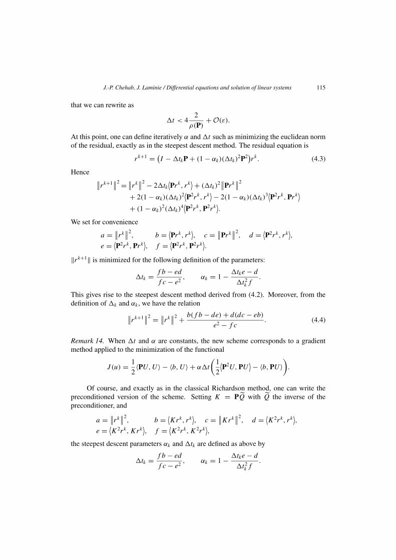
that we can rewrite as

�t < 42

ρ(P)+ O(ε).

At this point, one can define iteratively α and �t such as minimizing the euclidean normof the residual, exactly as in the steepest descent method. The residual equation is

rk+1 = (I − �tkP + (1 − αk)(�tk)

2P2)rk. (4.3)

Hence∥∥rk+1

∥∥2 = ∥

∥rk∥∥2 − 2�tk

⟨Prk, rk

⟩ + (�tk)2∥∥Prk

∥∥2

+ 2(1 − αk)(�tk)2⟨P2rk, rk

⟩ − 2(1 − αk)(�tk)3⟨P2rk, Prk

⟩

+ (1 − αk)2(�tk)

4⟨P2rk, P2rk

⟩.

We set for convenience

a = ∥∥rk

∥∥2

, b = ⟨Prk, rk

⟩, c = ∥

∥Prk∥∥2

, d = ⟨P2rk, rk

⟩,

e = ⟨P2rk, Prk

⟩, f = ⟨

P2rk, P2rk⟩.

‖rk+1‖ is minimized for the following definition of the parameters:

�tk = f b − ed

f c − e2, αk = 1 − �tke − d

�t2k f

.

This gives rise to the steepest descent method derived from (4.2). Moreover, from thedefinition of �k and αk, we have the relation

∥∥rk+1

∥∥2 = ∥

∥rk∥∥2 + b(f b − de) + d(dc − eb)

e2 − f c. (4.4)

Remark 14. When �t and α are constants, the new scheme corresponds to a gradientmethod applied to the minimization of the functional

J (u) = 1

2〈PU, U〉 − 〈b, U〉 + α�t

(1

2

⟨P2U, PU

⟩ − 〈b, PU〉)

.

Of course, and exactly as in the classical Richardson method, one can write thepreconditioned version of the scheme. Setting K = PQ̃ with Q̃ the inverse of thepreconditioner, and

a = ∥∥rk

∥∥2

, b = ⟨Krk, rk

⟩, c = ∥

∥Krk∥∥2

, d = ⟨K2rk, rk

⟩,

e = ⟨K2rk, Krk

⟩, f = ⟨

K2rk, K2rk⟩,

the steepest descent parameters αk and �tk are defined as above by

�tk = f b − ed

f c − e2, αk = 1 − �tke − d

�t2k f

.


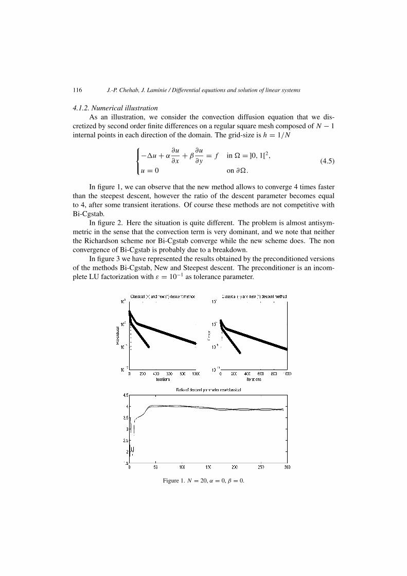
4.1.2. Numerical illustrationAs an illustration, we consider the convection diffusion equation that we dis-

cretized by second order finite differences on a regular square mesh composed of N − 1internal points in each direction of the domain. The grid-size is h = 1/N

−�u + α∂u

∂x+ β

∂u

∂y= f in � = ]0, 1[2,

u = 0 on ∂�.

(4.5)

In figure 1, we can observe that the new method allows to converge 4 times fasterthan the steepest descent, however the ratio of the descent parameter becomes equalto 4, after some transient iterations. Of course these methods are not competitive withBi-Cgstab.

In figure 2. Here the situation is quite different. The problem is almost antisym-metric in the sense that the convection term is very dominant, and we note that neitherthe Richardson scheme nor Bi-Cgstab converge while the new scheme does. The nonconvergence of Bi-Cgstab is probably due to a breakdown.

In figure 3 we have represented the results obtained by the preconditioned versionsof the methods Bi-Cgstab, New and Steepest descent. The preconditioner is an incom-plete LU factorization with ε = 10−1 as tolerance parameter.

Figure 1. N = 20, α = 0, β = 0.


Figure 2. N = 20, α = 104, β = 102.

Figure 3. N = 25, α = 105, β = 0.


5. Numerical results

5.1. Self-preconditioning

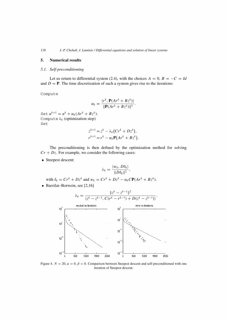
Let us return to differential system (2.4), with the choices A = 0, B = −C = Idand D = P. The time discretization of such a system gives rise to the iterations:

Compute

αk = 〈rk, P(Ark + Bzk)〉‖P(Ark + Bzk)‖2

.

Set uk+1 = uk + αk(Ark + Bzk).Compute λk (optimization step)Set

zk+1 = zk − λk

(Crk + Dzk

),

rk+1 = rk − αkP(Ark + Bzk

).

The preconditioning is then defined by the optimization method for solvingCr + Dz. For example, we consider the following cases:

• Steepest descent:

λk = 〈wk, Dδk〉‖Dδk‖2

,

with δk = Crk + Dzk and wk = Crk + Dzk − αkCP(Ark + Bzk).

• Barzilai–Borwein, see [2,16]

λk = ‖zk − zk−1‖2

〈zk − zk−1, C(rk − rk−1) + D(zk − zk−1)〉 .

Figure 4. N = 20, α = 0, β = 0. Comparison between Steepest descent and self-preconditioned with oneiteration of Steepest descent.


Figure 5. N = 20, α = 0, β = 0. Comparison between steepest descent and self-preconditioned with oneiteration of Barzilai–Borwein.

• Spectral gradient method λk = β−1k with

βk = (−βk−1)〈zk − zk−1, C(rk − rk−1) + D(zk − zk−1)〉

‖zk − zk−1‖2.

Of course, one can improve the preconditioning step by doing more than 1 it-eration of the optimization step Barzilai–Borwein (BB) or Steepest Method (SM), forinstance.

We have summarized in the following table the results for the Dirichlet problemdiscretized with a uniform mesh with 30 points in each direction of the domain).

# iterations Self-preconditioning CG Steepest descent

of BB/methodouter iterations total iterations

1 1145 1145 61 3960

2 460 916

3 259 771

4 232 920

10 115 1130

5.2. Shooting methods

Let us consider the subdivision of [0, T ] into N equal subintervals. The flow func-tion F : z(0) �→ r(T ) is approached by computing r(T ) with M iterations of a giventime marching scheme with �t = T/M as time step. We denote by FN the underlyingdiscrete flow function. At this point the problem consists in computing a zero of FN ;


this task can be accomplished any optimization method:{

For k = 0 . . .

zk+10 = zk

0 − αkGkFN

(zk

0

).

Here αk is a real number and Gk is a matrix, so the classical methods (Newton [17],Barzilai–Borwein [16], etc.) enter in this framework.

If the optimization method is chosen to be Barzilai–Borwein, we obtain thescheme:

Compute FN(zk) asSet rk,0 = rk, zk,0 = zk for m = 1 to M

{rk,m = rk,m−1 − �tPzk,m−1,

zk,m = zk,m−1 + �t(−zk,m−1 + rk,m−1 − Pzk,m−1

)

Set rk,N = rk+1, zk,N = zk+1

Compute

λk = ‖zk − zk−1‖2

〈zk − zk−1,FN(zk) − FN(zk−1)〉Set zk+1 = zk − λkFN(zk).

In practice, we chose �t as the optimal relaxation parameter of the associatedRichardson method, namely, �t = 2/(µ + ) where µ (resp. ) is the magnitude ofthe smallest (resp. the largest) eigenvalue of the matrix in magnitude. We observed thatthis choice gives better results.

In figure 6 we have compared the solution of the Poisson equation, comparing GM-RES(10), Bi-Cgstab and the shooting method with 2 time steps (�t = 6.1035e−05) withthe Barzilai–Borwein scheme for computing iteratively the root of the flow function, asdescribed above.

We observe that the coupled method shooting/BB converges faster than BB itselfand that it requires less matrix–vector product (536 vs 620): BB is accelerated by theshooting coupling.

In figure 7 we have compared the solution of the convection–diffusion equationwhen applying first, Bi-Cgstab and the shooting method with 2 time steps (�t =5.9167e−05) and after when using the Barzilai–Borwein scheme for computing iter-atively the root of the flow function, as described above.

The classical BB scheme does not converge while the coupled BB-S does. Thecoupling with the shooting method stabilizes then the original BB scheme.

In figure 8 we have realized a similar simulation, but here the convection termis more important (10000ux) and the number of grid points per direction of the domainis 63. We compare the coupled shooting method – Barzilai–Borwein scheme (with �t =3.0871e−06) with GMRES(10).


Figure 6. Solution of −�u = f , ]0, 1[2, u|∂� = 0 by GMRES(10), Bi-Cgstab and by the shooting method;63 grid points per direction of the domain.

6. Concluding remarks

The dynamical system approach to the solution of linear systems we have presentedhere allows to recover classical methods but also to introduce new ones. This approachis versatile thanks to its modularity since two degrees of freedom are needed, one for thedefinition of the (continuous) dynamical system and the other for the choice of the timemarching scheme that can be treated in many different manners, e.g., by using an ODEtoolbox. This is, in fact, a kind of arte povera in numerical analysis: many of existing


Figure 7. Solution of −�u + 1000ux = f , ]0, 1[2, u|∂� = 0 by Bi-Cgstab and by the shooting method.

iterative schemes, not necessary aimed at solving linear systems, can be (re-)used forcomposing a new method. Finally, the analysis of the numerical methods can be easilyaccomplished by using tools and concepts of numerical analysis of ODEs instead oftools of linear algebra only, mainly Krylov spaces techniques.

The schemes we have obtained are of numerical interest: they are stable (as ob-served in the solution of dominant convective problems) and the coupling with shootingmethods allows to stabilize optimizations schemes. Of course, we have studied heresimple models but many further developments can be considered, involving more com-plex situations, such as the modeling of a problem by an ODE can apply to nonlinearproblems, see [1, and the references therein].

The dynamical system approach can be applied advantageously for deriving newnumerical schemes and for studying their convergence in a simple way; it suggests toconsider the numerical linear algebra not only through the Krylov methods.


Figure 8. Solution of −�u + 10000ux = f , ]0, 1[2, u|∂� = 0 by Bi-Cgstab, GRMES(10) and by theshooting method.

References

[1] F. Alvarez, H. Attouch, J. Bolte and P. Redont, A second-order gradient-like dissipative dynamicalsystem with Hessian-driven damping. Application to optimization and mechanics, J. Math. PuresAppl. 81 (2002) 747–779.

[2] J. Barzilai and J.M. Borwein, Two points step size gradient methods, IMA J. Numer. Anal. 8 (1988)141–148.

[3] M. Benzi, Preconditioning techniques for large linear systems: A survey, J. Comput. Phys. 182 (2002)418–477.

[4] A. Bhaya and E. Kaszkurewicz, Iterative methods as dynamical systems with feedback control,Preprint, UFRJ, Department of Electrical Engineering (2003).


[5] C. Brezinski, Variations on Richardson’s method and acceleration, in: Numerical Analysis.A Numerical Analysis Conference in Honour of Jean Meinguet, Bull. Soc. Math. Belg. (1996)pp. 33–44.

[6] C. Brezinski, Projection Methods for Systems of Equations (North-Holland, Amsterdam, 1997).[7] C. Brezinski, Difference and differential equations, and convergence acceleration algorithms, in:

SIDE III – Symmetries and Integrability of Difference Equations, eds. D. Levi and O. Ragnisco, CRMProceedings and Lecture Notes, Vol. 25 (AMS, Providence, RI, 2000).

[8] C. Brezinski, Dynamical systems and sequence transformations, J. Phys. A: Math. Gen. 34 (2001)10659–10669.

[9] C. Brezinski and J.-P. Chehab, Nonlinear Hybrid Procedures and fixed point iterations, Numer. Funct.Anal. Optim. 19 (1998) 465–487.

[10] J.-P. Chehab, Differential equations and inverse preconditioners, Prépublications d’Orsay 2002-20,submitted.

[11] A. Cuyt and L. Wuytack, Nonlinear Methods in Numerical Analysis (North-Holland, Amsterdam,1987).

[12] R.W. Freund and N.M. Nachtigal, QMR a quasi-minimal residual method for non-Hermitian linearsystems, Numer. Math. 60 (1991) 315–339.

[13] U. Helmke and J.B. Moore, Optimization and Dynamical Systems (Springer, Berlin, 1994).[14] M.W. Hirsch and S. Smale, Differential Equations, Dynamical Systems and Linear Algebra

(Academic Press, London, 1974).[15] J.H. Hubbard and B.H. West, Differential Equations. A Dynamical Systems Approach. Part I: Ordi-

nary Differential Equations (Springer, New York, 1991).[16] F. Luengo, M. Raydan, W. Glunt and T.L. Hayden, Preconditioned spectral gradient method, Numer.

Algorithms 30 (2002) 241–258.[17] J.M. Ortega and W.C. Rheinboldt, Iterative Solution of Nonlinear Equations in Several Variables

(Academic Press, San Diego, 1970).[18] Y. Saad, Iterative Methods for Sparse Linear Systems (SIAM, Philadelphia, PA, 1996).[19] A.M. Stuart, Numerical analysis of dynamical systems, in: Acta Numerica (Cambridge Univ. Press,

Cambridge, 1994) pp. 467–572.[20] H.A. Van der Vorst, Bi-Cgstab: A fast and smoothly converging variant of Bi-CG for the solution of

nonsymmetric linear systems, SIAM J. Sci. Statist. Comput. 13 (1992) 631–644.

Documents

Differential equations and solution of linear systemsmath.univ-lille1.fr/~chehab/Rech/chehablaminie.pdf · 2007-04-06 · J.-P. Chehab, J. Laminie / Differential equations and solution