Embed Size (px)
Citation preview

Differential cross-section measurements
of the associated production of top
quarks with a photon at 13 TeV with the
ATLAS detector
DISSERTATIONzur Erlangung des Grades eines
Doktors der Naturwissenschaften
(Dr. rer. nat.)
vorgelegt vonJohn Meshreki, M.Sc.
ausAlexandria, Ägypten
eingereicht bei der Naturwissenschaftlich-Technischen Fakultätder Universität Siegen
Siegen 2021

Betreuer und erster Prof. Dr. Ivor FleckGutachter: Universität Siegen
Zweiter Gutachter: Prof. Dr. Markus CristinzianiUniversität Siegen
Tag der Disputation: 15.06.2021

Acknowledgements
I would like to sincerely thank my supervisor Prof. Dr. Ivor Fleck for giving me theopportunity to pursue my doctoral research at one of the top-tier experiments at CERN, whichwas a dream to me since I was a bachelor student and first heard about CERN and all theexciting research done there. I am most grateful for my supervisor’s continuous supportand for all the skills and professional experiences I built as a member of his group, and forsupporting me to attend workshops and conferences in Germany and abroad. I would alsolike to thank Prof. Dr. Markus Cristinziani for reviewing and grading my thesis as the secondreviewer as well as the other members of my Ph.D. committee, Prof. Dr. Markus Risse andProf. Dr. Wolfgang Kilian.
I am thankful to all my colleagues in Siegen, Göttingen, Bonn and CERN with whomI collaborated over the years, learnt from and made this work possible. I would like tothank Dr. Carmen Diez Pardos for the day-to-day supervision, numerous discussions andhelpful feedback, for pushing forward the analysis leading to a publication, and for her carefulrevision and comments on the thesis’ draft which helped me to improve its quality. I wouldlike to take this opportunity to express my gratitude to Dr. Yichen Li who helped me a lot ingaining technical skills as well as simplifying many of the new topics I faced at the beginningof my Ph.D. I can not thank you enough for all the support you gave me. I was also lucky tohave wonderful, cheerful, and supportive colleagues in my �푡�푡�훾 Siegen group. I would liketo thank Amartya Rej and Binish Batool for all the countless discussions and all the funmoments we shared in the office and in the schools and conferences we attended together.I am also thankful to Dr. Knut Zoch for his contribution to the �푡�푡�훾 �푒�휇 analysis as the leadanalyser for the inclusive measurement.
I would like to express my gratitude to all my friends and especially Andreas Albu whohas been there for me all along and supported me as a true, honest and reliable friend.
Last but not least, I would like to thank my family for making the impossible possibleand for their constant encouragement and support. I would like to express my fullest anddeepest gratitude to my mother for helping me achieve my dreams and for all the sacrificesshe made so that my dreams come true. I am also very fortunate and ever grateful for havingmy beloved wife Reham who supported me in all the difficult times and has always believedin me and I am thankful to her for consistently giving me hope and strength to keep on goingforward claiming my dreams.
iii


Abstract
Absolute and normalised differential cross-sections for the associated production of topquarks with a photon are measured in proton-proton collisions data at a centre-of-mass energyof 13 TeV. The data were collected by the ATLAS detector during the full Run 2 of theLHC with an integrated luminosity of 139 fb
−1. The measurements are performed in theelectron-muon decay channel in a fiducial phase space at parton level. The signal region ischaracterised by events with exactly one hard photon, one electron and one muon of oppositecharge, at least two jets, among which at least one is �푏-tagged, and missing transverse energy.The differential cross-sections are measured as functions of photon kinematic observables,the minimum angular distance between the photon and the leptons, and angular separationsbetween the two leptons. The results are compared to the most recent theory prediction atnext-to-leading-order accuracy in QCD and state-of-the-art Monte Carlo simulations. Themeasurements are found to be in agreement with the Standard Model predictions withinuncertainties.
v

Zusammenfassung
Absolute und normalisierte differentielle Wirkungsquerschnitte für die assoziierte Produk-tion von Top-Quarks mit einem Photon bei Proton-Proton-Kollisionen mit einer Schwerpunkt-senergie von 13 TeV werden gemessen. Die Daten wurden vom ATLAS-Detektor währenddes gesamten Laufs 2 des LHC mit einer integrierten Luminosität von 139 fb
−1 aufgezeich-net. Die Messungen werden im Elektron-Muon-Zerfallskanal in einem wohldefiniertenPhasenraum auf Partonenebene durchgeführt. Der Signalbereich ist charakterisiert durchein hochenergetisches Photon, ein Elektron und ein Myon mit entgegengesetzter Ladung,mindestens zwei Jets, von denen mindestens einer �푏-tagged ist, und fehlenden transversalenImpuls. Die differentiellen Wirkungsquerschnitte werden als Funktionen kinematischerObservablen des Photons, des minimalen Winkelabstands zwischen dem Photon und denLeptonen, und Winkelabstände zwischen den beiden Leptonen gemessen. Die Ergebnissewerden mit der neuesten Theorievorhersage mit NLO-Genauigkeit in QCD und dem Standder Technik entsprechenden Monte-Carlo-Simulationen verglichen. Die Messungen sind inÜbereinstimmung mit den Vorhersagen des Standardmodells im Rahmen der Unsicherheiten.
vi


Contents
1 Introduction 1
2 Top quark at the Standard Model 3
2.1 The Standard Model . . . . . . . . . . . . . . . . . . . . . . . . . . . . . 32.2 Top-quark physics . . . . . . . . . . . . . . . . . . . . . . . . . . . . . . . 72.3 Top-quark production in association with photons . . . . . . . . . . . . . . 10
3 Experimental Setup 15
3.1 The ATLAS detector . . . . . . . . . . . . . . . . . . . . . . . . . . . . . 173.1.1 Coordinates of the detector . . . . . . . . . . . . . . . . . . . . . . 183.1.2 Magnet systems . . . . . . . . . . . . . . . . . . . . . . . . . . . . 193.1.3 Inner Detector . . . . . . . . . . . . . . . . . . . . . . . . . . . . 193.1.4 Calorimeters . . . . . . . . . . . . . . . . . . . . . . . . . . . . . 213.1.5 Muon Spectrometer . . . . . . . . . . . . . . . . . . . . . . . . . . 213.1.6 Trigger system . . . . . . . . . . . . . . . . . . . . . . . . . . . . 23
4 Object definition 25
4.1 Electrons . . . . . . . . . . . . . . . . . . . . . . . . . . . . . . . . . . . 254.1.1 Reconstruction . . . . . . . . . . . . . . . . . . . . . . . . . . . . 254.1.2 Identification and isolation . . . . . . . . . . . . . . . . . . . . . . 26
4.2 Muons . . . . . . . . . . . . . . . . . . . . . . . . . . . . . . . . . . . . . 274.2.1 Reconstruction . . . . . . . . . . . . . . . . . . . . . . . . . . . . 274.2.2 Identification and isolation . . . . . . . . . . . . . . . . . . . . . . 29
4.3 Photons . . . . . . . . . . . . . . . . . . . . . . . . . . . . . . . . . . . . 304.3.1 Reconstruction . . . . . . . . . . . . . . . . . . . . . . . . . . . . 304.3.2 Identification and isolation . . . . . . . . . . . . . . . . . . . . . . 304.3.3 Shower shapes reweighting . . . . . . . . . . . . . . . . . . . . . . 31
4.4 Jets . . . . . . . . . . . . . . . . . . . . . . . . . . . . . . . . . . . . . . 314.4.1 Reconstruction . . . . . . . . . . . . . . . . . . . . . . . . . . . . 314.4.2 Calibration . . . . . . . . . . . . . . . . . . . . . . . . . . . . . . 324.4.3 �푏-tagging . . . . . . . . . . . . . . . . . . . . . . . . . . . . . . . 33
4.5 Missing transverse energy . . . . . . . . . . . . . . . . . . . . . . . . . . . 34
ix

5 Shower shapes reweighting for photons 37
5.1 Data and MC samples . . . . . . . . . . . . . . . . . . . . . . . . . . . . . 375.2 Cell-based energy reweighting of photons . . . . . . . . . . . . . . . . . . 375.3 Event selection . . . . . . . . . . . . . . . . . . . . . . . . . . . . . . . . 385.4 Pure �푍 → �푒�푒�훾 sample . . . . . . . . . . . . . . . . . . . . . . . . . . . . 385.5 Results of cell-based reweighting . . . . . . . . . . . . . . . . . . . . . . . 42
5.5.1 Background reduction . . . . . . . . . . . . . . . . . . . . . . . . 425.5.2 Cell-based energy reweighting . . . . . . . . . . . . . . . . . . . . 42
6 Data and MC simulation for �풕 �풕�휸 + �풕�푾�휸 measurement 49
6.1 Data . . . . . . . . . . . . . . . . . . . . . . . . . . . . . . . . . . . . . . 496.2 MC simulation . . . . . . . . . . . . . . . . . . . . . . . . . . . . . . . . 496.3 Simulation of signal . . . . . . . . . . . . . . . . . . . . . . . . . . . . . . 516.4 Simulation of background processes . . . . . . . . . . . . . . . . . . . . . 526.5 Overlap removal between samples . . . . . . . . . . . . . . . . . . . . . . 54
7 Object and event selection 55
7.1 Object-level selection . . . . . . . . . . . . . . . . . . . . . . . . . . . . . 557.2 Event-level selection . . . . . . . . . . . . . . . . . . . . . . . . . . . . . 56
8 Analysis strategy 61
8.1 Fiducial phase-space definition . . . . . . . . . . . . . . . . . . . . . . . . 618.2 Differential cross-sections . . . . . . . . . . . . . . . . . . . . . . . . . . 638.3 Unfolding methodology . . . . . . . . . . . . . . . . . . . . . . . . . . . . 69
8.3.1 Iterative Bayesian unfolding . . . . . . . . . . . . . . . . . . . . . 708.3.2 Binning optimisation . . . . . . . . . . . . . . . . . . . . . . . . . 718.3.3 Performance and optimisation studies using pseudo-data . . . . . . 77
9 Systematic uncertainties 87
9.1 Experimental uncertainties . . . . . . . . . . . . . . . . . . . . . . . . . . 889.2 Modelling uncertainties . . . . . . . . . . . . . . . . . . . . . . . . . . . . 91
10 Results 95
10.1 Absolute cross-section measurements . . . . . . . . . . . . . . . . . . . . 9510.2 Normalised cross-section measurements . . . . . . . . . . . . . . . . . . . 107
11 Conclusions and outlook 119
Bibliography 121
A Additional shower shapes and fit results 133
B Additional cross-section results 151
x

CHAPTER 1
Introduction
The Standard Model (SM) of elementary particles is the most successful theory to date indescribing the building blocks of the universe and their interactions. Its current structurewas completed in the 1970s, and since then, its predictions have been extensively tested.Through these experimental tests, all predictions of the SM have been confirmed. Despite itsimpressive success, however, the SM is not a final theory. For example, it does not explainthe matter-antimatter asymmetry and does not yet include the gravitational force. Theseunreconciled topics, among others, are the main drive to continuously test predictions of theSM to the best achievable accuracy and simultaneously search for hints of new physics.
One of the pillars of the SM is the top quark. It is the heaviest elementary particle andthe last quark to be discovered, found at the Tevatron Collider in 1995 [1, 2]. Its heavymass implies a large Yukawa coupling to the Higgs boson, which points to its unique role inthe electroweak symmetry breaking of the SM. The top quark has a very short lifetime anddecays before hadronisation, allowing for studying its properties through its decay products.One of these properties is the electroweak coupling between the top quark and the photon.Such coupling can be probed at the Large Hadron Collider (LHC) by studying the associatedproduction of a top-quark pair with a photon (�푡�푡�훾).
The evidence of the �푡�푡�훾 process was found with a 3.0 �휎 significance at the TevatronCollider in proton-antiproton (�푝�푝) collisions at centre-of-mass energy (
√�푠) of 1.96 TeV, with
an integrated luminosity of 6 fb−1 in 2011 [3]. The �푡�푡�훾 process was later observed by the
ATLAS experiment in proton-proton (�푝�푝) collisions at√�푠 = 7 TeV at the LHC in 2015 [4].
The observation was perfomred in the lepton+jets channel with an integrated luminosity of4.59 fb
−1 and achieved a 5.0 �휎 significance. In 2017, the ATLAS experiment performed thefirst differential �푡�푡�훾 measurement at
√�푠 = 8 TeV with an integrated luminosty of 20.2 fb
−1 [5].In the same year and at the same
√�푠 of 8 TeV, the CMS experiment measured the ratio of
cross-sections of �푡�푡�훾 to �푡�푡 with an integrated luminosity of 19.7 fb−1 [6]. In 2019, the inclusive
and differential �푡�푡�훾 cross-sections were measured in both the single lepton and dileptonchannels. The measurements were performed by the ATLAS experiment at
√�푠 = 13 TeV
using collisions data with an integrated luminosity of 36.1 fb−1 [7]. This thesis presents the
1
Chapter 1 Introduction
most recent differential measurement of the production of top quarks in association with aphoton, performed in the �푒�휇 channel at
√�푠 = 13 TeV using data from the ATLAS experiment,
with an integrated luminosity of 139 fb−1 [8]. The measurements are compared for the first
time to a full calculation at next-to-leading order in Quantum Chromodynamics, whichincludes resonant and non-resonant diagrams, interferences, and off-shell effects of the topquark [9]. Hence, the signal process of the measurements is the combined �푡�푡�훾 productionand single top-quark production in association with a �푊 boson and a photon (�푡�푊�훾), which isreferred to as �푡�푡�훾 + �푡�푊�훾.
This thesis is organised as follows. Chapter 2 presents a brief overview of the SM anddiscusses the physics of the top quark and the production of the �푡�푡�훾 process. An overviewof the LHC and the experimental setup of the ATLAS detector is introduced in Chapter 3.A description of the algorithms used to reconstruct and select physics objects relevant tothis work is detailed in Chapter 4. In Chapter 5, a method to improve the agreement ofdistributions related to the energy deposits of photons (referred to as shower shapes) betweendata and Monte Carlo simulations is presented. The data and Monte Carlo samples ofsignal and backgrounds and the selection applied at an object- and event-levels are describedin Chapters 6 and 7, respectively. The fiducial phase-space definition, the strategy to performthe differential measurements, and the unfolding procedure and related studies are detailedin Chapter 8. Chapter 9 describes the systematic uncertainties considered in this work. Theresults of the absolute and normalised cross-sections are reported in Chapter 10, which isfollowed by conclusions and an outlook in Chapter 11.
Natural units are used throughout this thesis, ℏ = �푐 = 1, where ℏ and �푐 are the reducedPlanck constant and speed of light in vacuum, respectively. The electric charge of particles ismeasured in units of the elementary charge (e). Masses, momenta and energies of particlesare measured in units of electronvolt (eV) and its (metric prefixes) multiples such as MeV,GeV and TeV.
2
CHAPTER 2
Top quark at the Standard Model
2.1 The Standard Model
The SM is a theory that describes elementary particles and their interactions at the mostminiature scale. It uses a quantum field formalism which describes particles as excitationstates of the corresponding quantum field; hence, it is a Quantum Field Theory (QFT). Itincludes three fundamental forces of nature: the strong force mediated by the exchange ofthe massless and electrically neutral gluons, the weak force mediated by the exchange of themassive neutral �푍 bosons and charged �푊 bosons, and the electromagnetic force mediatedby the massless and electrically neutral photons. The theory of Quantum Chromodynamics(QCD) [10–12] describes the strong force, whereas the weak and electromagnetic forcesare unified together and described by the electroweak theory [13–15]. The gauge symmetrygroup of the SM have the structure:
�푆�푈 (3)�퐶 ⊗ �푆�푈 (2)�퐿 ⊗ �푈 (1)�푌 , (2.1)
where �푆�푈 (3)�퐶 is the gauge group of QCD and �푆�푈 (2)�퐿 ⊗ �푈 (1)�푌 is the gauge group of theelectroweak interaction. The subscript �퐶 refers to colour charge, whereas the subscripts �퐿and �푌 refer to left-handed isospin and hypercharge, respectively. The fourth force of nature,which is the gravitational one, is not included in the SM.
Elementary particles are considered the building blocks, hence, the name elementary, ofthe visible matter of our universe, which comprises only around 5% of the total density of theuniverse. There are twelve fermions in the SM, where fermions are particles with half-integerspin. Such particles interact by exchanging one of five particles called gauge bosons, particleswith integer spin. Fig. 2.1 display all these elementary particles of the SM.
There are two types of fermions: leptons and quarks. They are classified into three familiesor generations, which increase in mass when going from the first to the third generation.Leptons that are electrically charged have a charge of 1 e. Such charged leptons are electrons,muons, and taus which are denoted as �푒, �휇, and �휏, respectively. Both muons and taus are
3

Chapter 2 Top quark at the Standard Model
Figure 2.1: Overview of elementary particles in the SM. Three families of fermions, along with thegauge and Higgs bosons, are shown. The figure is sourced from Ref. [16] and modified.
unstable particles, and they decay spontaneously, whereas the electron is stable. Furthermore,leptons in each generation form a weak isospin doublet where each charged lepton has acorresponding electrically neutral particle called a neutrino, e.g. the �푒 forms with the electronneutrino (�휈�푒) an isospin doublet. The muon neutrino and tau neutrino are denoted as �휈�휇 and�휈�휏, respectively. Moreover, charged leptons have their corresponding antiparticles, whichhave the same mass and spin but an opposite sign of the relevant quantum numbers, e.g. theelectron has an electric charge of -1 e, whereas its antiparticle, the positron, has a chargeof +1 e. Neutrinos are distinguished from their corresponding antiparticles, denoted asantineutrinos, by differing in the sign of the lepton number and the chirality of the particle(right- or left-handed). For simplicity, charged leptons hereafter are called leptons, andthey refer to particles and their corresponding antiparticles as well, unless explicitly statedotherwise.
Quarks have a non-integer electric charge of either +2/3 e such as the up, charm, and
4

2.1 The Standard Model
top quarks, denoted as �푢, �푐, and �푡, respectively, or -1/3 e such as the down, strange, andbottom quarks, denoted as �푑, �푠, and �푏, respectively. Like leptons, quarks are also groupedinto weak isospin doublets that differ by one unit of electric charge, e.g. the up and downquarks. In addition to an electric charge, quarks have a colour charge. Quarks also have theircorresponding antiparticles, called antiquarks, e.g. the antitop and antibottom quarks denotedas �푡 and �̄푏, respectively.
The strong interaction
The strong force is, as the name suggests, the most potent force of nature. It acts at theshortest distances and is responsible for holding the protons together in the nucleus, despitetheir electric repulsion. Furthermore, it is also responsible for holding together the quarksinside the proton or the neutron.
The quantum number of the strong interaction is called colour, and it has three states: red,green, and blue. Quarks carry one unit of colour charge, while antiquarks carry one unit ofanticolour. Gluons carry one unit of colour and one unit of anticolour, and they exist in anoctet of linear combinations of the three colours. Since gluons are colour charged, they caninteract with one another in addition to their interactions with the quarks.
The strength of the strong interaction is determined by the strong coupling constant (�훼�푆).The coupling constant is also called running coupling constant, since it is not a constantquantity but rather runs with respect to the four-momentum transfer (�푄):
�훼�푆 (�푄2) = 12�휋
(33 − 2n �푓 ) log(Q2/Λ2QCD)
, (2.2)
where n �푓 is the number of quark flavors and ΛQCD is the fundamental scale of QCD whichallows the evaluation of the coupling constant at a scale of �푄 > ΛQCD.
The dependence of �훼�푆 on �푄, which can be seen in Fig. 2.2, probes two characteristicproperties of QCD:
• Colour confinement which states that at small �푄2, colour-charged particles —quarksand gluons—cannot exist as isolated particles. When quarks are pulled apart, thepotential energy increases so that it is enough to produce quark and antiquark pairs,forming colourless bound-states called hadrons. There are two types of hadrons, mesonsconsisting of a quark and an antiquark, and baryons composed of either three quarksor three antiquarks. The process of forming hadrons is called hadronisation which isdescribed in Chapter 6.
• Asymptotic freedom which states that at large �푄2, quarks and gluons interact weakly orbehave like free particles [18].
5

Chapter 2 Top quark at the Standard Model
Figure 2.2: Summary of measurements of �훼�푆 as a function of �푄. The respective degree of QCDperturbation theory is indicated in parenthesis. The figure is sourced from Ref. [17].
The electroweak interaction
The theories of Quantum Electrodynamics (QED) and weak interactions were initiallydeveloped separately. The electromagnetic interaction describes the interactions betweenelectrically charged particles through mediating photons. The strength of the electromagneticforce is represented by the coupling constant (�푔�푒), which is expressed as �훼�푒:
�훼�푒 =�푔
2�푒
4�휋≈ 1
137(2.3)
The weak interaction describes the interactions of particles via mediating charged �푊±
bosons (also denoted simply as �푊 bosons) or neutral �푍 bosons. Leptons do not participatein the strong interaction since they do not carry colour, and neutrinos do not interactelectromagnetically, as they have no electric charge. However, all leptons and quarks interactweakly, i.e. participate in the weak interaction.
In the 1960s, a gauge-invariant theory was constructed, which combined the electromagneticand weak forces. This unification of forces was the work of Glashow [13], Salam [14], andWeinberg [15], which is referred to as the electroweak unification. The resulting electroweak
6

2.2 Top-quark physics
interaction is described by the �푆�푈 (2)�퐿 ⊗ �푈 (1)�푌 symmetry group. The gauge symmetryrequires the �푊 and �푍 bosons to be massless, although experimentally, they are observed to bemassive [19]. The origin of their masses was understood by introducing another quantum field,the so-called Higgs field [20–23], which leads to the spontaneous breaking of the electroweaksymmetry. The Higgs field was introduced as a complex scalar SU(2) doublet. Through theelectroweak symmetry breaking, fermions acquire their masses through interactions withthe Higgs field, where their masses are proportional to the vacuum expectation value of theHiggs field and the corresponding Yukawa coupling. Quantum excitation of the Higgs fieldproduces the Higgs boson, which was was discovered experimentally in 2012 by ATLAS [24]and CMS [25].
2.2 Top-quark physics
The top quark is the heaviest elementary particle in the SM with a mass of 173.34 ±0.76 GeV [26]. Its heavy mass provides access to the largest Yukawa coupling, which ispredicted to be close to unity. This points to its unique role in validating predictions ofthe SM. Furthermore, it has a very short lifetime of 10
−24s. This remarkably brief record
permits it to decay before forming a bound state, which allows measuring its properties byexamining its decay products. One of these properties which is accessible experimentally andnot washed out by hadronisation is the spin information of the top quark. The top-quark pair(�푡�푡) spin correlation can be probed through the angular distributions of the decay productsof the �푡 and �푡 (see Section 8.2 for observables that are sensitive to the �푡�푡 spin correlation).Deviations from the angular distributions predicted by the SM would indicate new physics.
Production of top-quark pairs
At hadron colliders, top quarks are produced in pairs or as a single top, where the former isthe dominant process. The �푡�푡 are produced predominantly through the strong interaction viagluon-gluon (�푔�푔) fusion and �푞�푞 annihilation, for which representative diagrams at leadingorder (LO) in QCD are shown in Fig. 2.3. At the LHC, 90% of the production is throughthe �푔�푔 fusion at
√�푠 = 14 TeV. The reason for such a high rate is that the �푞�푞 annihilation is
suppressed since antiquarks in protons exist only as sea quarks.
The �푡�푡 production cross-section can be calculated with the help of the factorisationtheorem [27]. This theorem separates the calculation of the long-distance interactions ofpartons from the short-distance ones (hard interaction) by introducing a factorisation scale(�휇�퐹). The value of �휇�퐹 is arbitrarily chosen, but it is typically set to the momentum transfer ofthe hard process. The hard interaction terms can be calculated with the perturbation theory,while the terms corresponding to the long-distance interactions are calculated using structurefunctions, known as Parton Distribution Functions (PDF) [28–30].
7

Chapter 2 Top quark at the Standard Model
Figure 2.3: Representative Feynman diagrams of the top-quark pair production at leading order inQCD via �푞�푞 annihilation (top left) and �푔�푔 fusion (top right and bottom).
Let two hadrons, �퐴 and �퐵, collide creating a final state �푋 . The inclusive cross-section forsuch a process is given as:
�휎�퐴�퐵→�푋 =
∑
�푎�푏
∫
�푥�푎
∫
�푥�푏
�푑�푥�푎�푑�푥�푏 �푓�푎,�퐴 (�푥�푎, �휇�퐹) �푓�푏,�퐵 (�푥�푏, �휇�퐹) × �̂휎�푎�푏→�푋 , (2.4)
where �̂휎�푎�푏→�푋 is the partonic cross-section of the hard interaction. The indices �푎 and �푏
represent partons in hadrons �퐴 and �퐵, respectively, where partons are valence quarks, seaquarks and gluons. The terms �푓�푎,�퐴 (�푥�푎, �휇�퐹) and �푓�푏,�퐵 (�푥�푏, �휇�퐹) are the PDFs of the hadrons�퐴 and �퐵, respectively, where �푥�푎 and �푥�푏 are the fractions of the momentum carried by thecorresponding parton. Therefore, the inclusive cross-section (�휎�푝�푝→�푡�푡) of �푝�푝 collisions to
create a final state of �푡�푡 can be calculated with Eq. (2.4). At√�푠 = 13 TeV, assuming a
top-quark mass of 172.5 GeV, �휎�푝�푝→�푡�푡 is predicted to be 831.8+19.8−29.2(scale)+35.1
−35.1(PDF) pb atthe LHC [17]. The cross-section is obtained at next-to-next-to-leading order (NNLO) in QCDand next-to-next-to-leading-logarithmic (NNLL) soft-gluon resummation with the TOP++2.0
program [31].
Production of single top quarks
The single top quark is produced via the electroweak interaction in three channels: �푠-channel, �푡-channel, and �푡�푊-channel, at LO in QCD. In the �푠-channel and �푡-channel, the
8

2.2 Top-quark physics
Figure 2.4: Representative Feynman diagrams of the single-top production at LO in QCD in the�푡-channel (top left), �푠-channel (top right), and �푡�푊-channel (bottom).
top quark is produced by the exchange of a virtual �푊 boson, whereas in the �푡�푊-channel, itis produced in association with a real �푊 boson. Examples of Feynman diagrams for thethree channels at LO in QCD are shown in Fig. 2.4. At
√�푠 = 13 TeV, assuming a top-quark
mass of 172.5 GeV, the cross-sections of the �푠-channel, �푡-channel, and �푡�푊-channel for thetop quark and antitop quark components at the LHC are 10.32
+0.29−0.24(scale)+0.27
−0.27(PDF) pb,
216.99+6.62−4.64(scale)+6.16
−6.16(PDF) pb, and 71.7+1.8−1.8(scale)+3.40
−3.40(PDF) pb, respectively [32]. Thecross-sections are obtained at NLO in QCD with the HATHOR (v2.1) program [33, 34].
Top-quark decay
The top quark decays via the weak interaction to a �푊 boson and a down-type quark (�푑, �푠,or �푏). The decay to a �푊 boson and a �푏-quark is the predominant process with a BranchingRatio (BR) close to 1 [35]. The decay to �푠- or �푑-quark is heavily suppressed owing to theirsubstantially weak mixing in the Cabibbo–Kobayashi–Maskawa matrix. The �푊 boson thendecays to leptons (a charged lepton and its corresponding neutrino) or quarks (a quark and anantiquark of the first two generations). Therefore, the �푡�푡 decay can be categorised in threedecay channels, for which the branching ratios are shown in Fig. 2.5, according to the decayproducts of the �푊 boson:
• Dileptonic: both �푊 bosons decay to two leptons: �푡�푡 → �푙+�휈�푙�푏�푙
−�̄휈�푙 �̄푏, where �푙 = �푒, �휇,
or �휏. This channel has the advantage of being very clean with the lowest backgroundcontamination. However, it has the smallest BR of 9%.
9

Chapter 2 Top quark at the Standard Model
Figure 2.5: Branching ratios of the �푡�푡 decay channels. The figure is sourced from Ref. [36] andmodified.
• All-hadronic: both �푊 bosons decay to two quarks: �푡�푡 → �푞1�푞2�푞3�푞4�푏�̄푏, where �푞 = �푢, �푑,�푠, or �푐. This channel has the largest BR of 46%, but it suffers from a large contributionof background processes.
• Single lepton or lepton+jets: one �푊 boson decays hadronically, whereas the other onedecays leptonically: �푡�푡 → �푙
+�휈�푙�푏�푞1�푞2�̄푏 or �푡�푡 → �푞1�푞2�푏�푙
−�̄휈�푙 �̄푏 where �푙 = �푒, �휇, or �휏 and
�푞 = �푢, �푑, �푠, or �푐. This channel is called the golden channel since it has a rather highBR of 45% while the background contamination is moderate.
2.3 Top-quark production in association with photons
The study of the �푡�푡�훾 process plays a vital role in testing predictions of the SM and possiblenew physics. For example, it has access to the �푡�훾 electroweak coupling. The SM predictssuch coupling, and deviation from such prediction would indicate new physics [37, 38].Furthermore, at the LHC, the �푡�푡�훾 couplings can be probed with a high precision (a fewper cent level), which allows to scrutinise the SM predictions and put constraints on theanomalous dipole moments of the top quark [37, 38]. Moreover, precise measurements of the�푡�푡�훾 permit interpretations in the context of effective field theories [39].
Photons being massless can be radiated from any electrically charged particle and not onlythe top quark. The �푡�푡�훾 process can be classified in two categories:
• In radiative top-quark production, the photon is radiated during the production of the �푡�푡.At LO in QCD, such production can occur in a �푞�푞 annihilation or a �푔�푔 fusion, as shownin the example diagrams of Fig. 2.6. The photon is radiated either from an incomingcharged parton or an off-shell top quark in these diagrams.
10
2.3 Top-quark production in association with photons
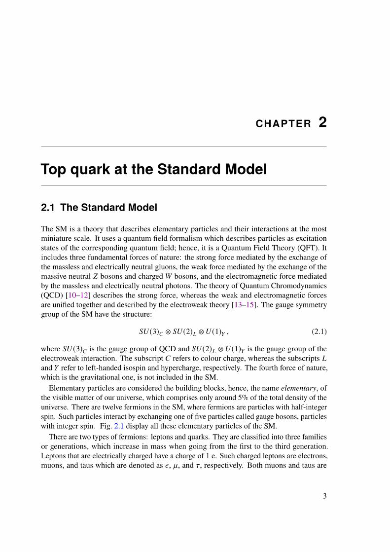
Figure 2.6: Representative Feynman diagrams at LO in QCD of the radiative top-quark production.The photon can be radiated from an off-shell top quark in �푞�푞 annihilation (top left) or �푔�푔 fusion (topright). The incoming partons can also emit the photon (bottom).
• In radiative top-quark decay, the photon is radiated from an on-shell top quark or anyof the electrically charged particles in the decay chain. Examples of Feynman diagramsare shown in Fig. 2.7. In the diagrams, the photon is emitted from the top quark, the�푏-quark, the �푊 boson, or the electrically charged decay product of the �푊 boson.
Both radiative production and decay of the top quark yield the same final state in thedetector.
A non-exhaustive summary of the theoretical calculations of the �푡�푡�훾 process is discussedin the following section, including the theory calculation used for comparison to themeasurements reported in this thesis.
Theory calculations
The earliest calculation of the �푡�푡�훾 process at next-to-leading order (NLO) in QCD wasperformed in 2009 [40]. This calculation used the Born approximation for top quarks,i.e. considering them as stable particles. Later in 2011, the �푡�푡�훾 calculation was furtherextended by considering a decaying top quark [41], i.e. including the two processes: radiativeproduction and decay of the top quark. When considering top quarks to be truly unstable,non-factorisable QCD corrections emerge [42–44]. The 2011 calculation [41] overcame suchan issue by treating the top quarks in the narrow width approximation. However, using the
11

Chapter 2 Top quark at the Standard Model
Figure 2.7: Representative Feynman diagrams at LO in QCD of the radiative top-quark decay. Thephoton can be radiated from the on-shell top quark (top left), the �푏-quark (top-middle), or the �푊
+
boson (top right). It can also be emitted from the electrically charged lepton, the �푙+ (bottom).
narrow width approximation means that off-shell contributions are neglected, and hence theinterference between the top-quark production and decay is ignored.
In 2018, the first full computation of the �푡�푡�훾 process at NLO in QCD was performed [9]. Itincluded resonant and non-resonant contributions, interferences, and off-shell effects of the topquark and the �푊 boson. This calculation considered the �푒�휇 final state: �푝�푝 → �푏�푒
+�휈�푒 �̄푏�휇
−�휈�휇�훾
at√�푠 = 13 TeV. Example Feynman diagrams of the double resonant, single resonant and
non-resonant top-quark diagrams are shown in Fig. 2.8. There are two top-quark resonancesin the double-resonant case, whereas there is only one top quark in the single resonant one. Inthe non-resonant case, no top-quark resonances are present. The three cases contribute to thesame final state of �푏�푒+�휈�푒 �̄푏�휇
−�휈�휇�훾. The top-quark mass was set to 173.2 GeV. The electroweak
coupling was derived from the Fermi constant �퐺�휇, where it was set to �훼�퐺�휇≈ 1/132. A value
of �훼 = 1/137 was used to describe the real photon emission. The calculation considered twoscenarios for the chosen factorisation (�휇�퐹) and normalisation (�휇�푅) scales. The first scenarioused a fixed scale for both scales, which were set to �휇�퐹 = �휇�푅 = �푚�푡/2 where �푚�푡 is the mass ofthe top quark. The second scenario used a dynamic scale, which was set to �휇�퐹 = �휇�푅 = �푆T/4.The �푆T is defined as the total transverse momentum of the system, i.e. the sum of transversemomenta of the leptons, photon, �푏-jets, and the missing transverse momentum from theescaping neutrinos. The second scenario was found to stabilise the shapes in the high regionof the transverse momentum of the photon and provided smaller theoretical uncertainties aswell. Therefore, it is chosen for the comparison with the measurements reported in this thesis.
The authors of Ref. [9] have done a dedicated recalculation in the fiducial phase spaceof the measurement (see Section 8.1). The NLO fiducial inclusive cross-section of the
12

2.3 Top-quark production in association with photons
Figure 2.8: Representative Feynman diagrams at LO in QCD of the double resonant (top left), singleresonant (top right), and non-resonant (bottom) top quark. The figure is sourced from Ref. [9].
process �푝�푝 → �푏�푒+�휈�푒 �̄푏�휇
−�휈�휇�훾 using the CT14 PDF set [45] and dynamical scale of �푆T/4 was
calculated to be:
�휎fid = 38.50+0.56−2.18 (scale) +1.04
−1.18 (PDF) fb (2.5)
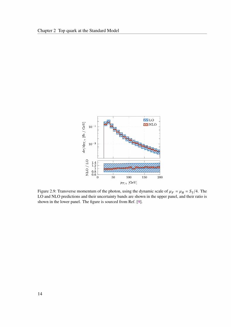
Besides the inclusive cross-section, the calculation also computed results of variousdifferential distributions at LO and NLO in QCD. Distributions as functions of observablesthat are relevant for searches beyond the SM were included. An example is the transversemomentum of the photon, which can be seen in Fig. 2.9. For such an observable, correctionsup to 13% is observed. The uncertainty bands in the figure also show that the NLO uncertaintyis smaller than the LO one.
13
Chapter 2 Top quark at the Standard Model
Figure 2.9: Transverse momentum of the photon, using the dynamic scale of �휇�퐹 = �휇�푅 = �푆T/4. TheLO and NLO predictions and their uncertainty bands are shown in the upper panel, and their ratio isshown in the lower panel. The figure is sourced from Ref. [9].
14

CHAPTER 3
Experimental Setup
LHC is the most powerful particle accelarator across the globe, which is built by the biggestlaboratory of high energy physics, CERN, the European Organization for Nuclear Research.The LHC has a 27 km circular tunnel, which lies approximately 120 m underground on theborder between France and Switzerland. It is a �푝�푝 collider which is designed to accelerate andcollide protons at
√�푠 = 14 TeV. It has four collision points at which four main experiments
are placed. The four experiments are A Toroidal LHC ApparatuS (ATLAS) [46, 47], CompactMuon Solenoid (CMS) [48], Large Hadron Collider beauty (LHCb) [49], and A Large IonCollider Experiment (ALICE) [50], which can be seen in Fig. 3.1. The ATLAS and CMSare called multipurpose detectors since they cover a broad spectrum of physics analyses.The LHCb experiment focuses on the physics of B hadrons, while ALICE investigates thequark-gluon plasma in heavy-ion collisions.
Physics analyses often use three quantities when describing physics processes at the LHC:
• The integrated luminosity (�퐿) : it is the number of collisions which are collected over acertain period of time interval and unit area. Its unit is expressed in the inverse of areaunits, e.g. inverse picobarn (pb−1
= 1040m−2) or inverse femtobarn (fb−1
= 1043m−2),
where barn is a metric unit of area (1 barn = 10−28m2). It is obtained by integrating the
instantaneous luminosity (�퐿inst) over the corresponding period of time (d�푡):
�퐿 =
∫
�퐿instd�푡 . (3.1)
The instantaneous luminosity is defined as:
�퐿inst =�푁
2�푏�푛
2�푏 �푓rev�훾
4�휋�휎�푥�휎�푦
�퐹 , (3.2)
15

Chapter 3 Experimental Setup
Figure 3.1: A schematic view of the accelerator complex at CERN. The LHC is the uppermost ring(dark grey ellipse) with the four main experiments (orange-colored circles) at the designed collisionpoints (©2008-2021 CERN). The figure is sourced from Ref. [51].
16

3.1 The ATLAS detector
where �푁�푏 is the number of particles per bunch, �푛�푏 is the number of bunches per beam,�푓rev is the revolution frequency, and �훾 is the relativistic gamma factor. The quantity�퐹 represents the geometric luminosity reduction factor, and �휎�푥 and �휎�푦 are the beamcross-sections in �푥 and �푦 directions, respectively.
• The cross-section (�휎): it represents the probability that an event or several events occuras a result of particles’ collisions with a given luminosity.
• The number of events (�푁): it is the expected number of events of a particular physicsprocess for a given cross-section and luminosity.
The relation between the three quantities can be expressed as:
�푁 = �휎 · �퐿 . (3.3)
3.1 The ATLAS detector
The ATLAS detector is constructed to perform precise measurements of the SM and beyond.One of its primary goals was to search for the Higgs boson, which was discovered in 2012 byboth experiments, ATLAS [24] and CMS [25].
The detector has an overall length of 44 m and a diameter of 25 m, weighing nearly7 × 10
6kg. It is constructed so that different subdetector systems are built in concentric
layers around the designed interaction point. The subdetector systems are classified into threesystems, as shown in Fig. 3.2:
• The Inner Detector (ID): it is the innermost part of the ATLAS detector, which iscontained within a cylindrical envelope surrounded by a solenoidal magnetic field. TheID is responsible for tracking the paths of charged particles, i.e. it acts as a trackingsystem. Besides, it measures their electric charge and momenta, as well as identifyingprimary and secondary interaction vertices. The vertex is called primary [52] whentwo protons collide with each other and secodary if it is associated with a decay of aparticle coming from the primary vertex.
• The calorimeters: they are placed outside the solenoidal magnetic field. They areresponsible for measuring the deposited energy of charged and neutral particles. Theyare designed to stop most of the particles that pass through except muons and neutrinos.
• The Muon Spectrometer (MS): it is the outermost part of the detector. It is immersed ina toroidal magnetic field and is responsible for measuring the properties of muons sincethey travel relatively longer distances than other particles and are less likely to interactwith other systems of the detector.
The coordinates of the detector and more details on the three subdetector systems aredescribed in the following sections.
17

Chapter 3 Experimental Setup
Figure 3.2: A schematic overview of the ATLAS detector. The figure is sourced from Ref. [53]
3.1.1 Coordinates of the detector
The ATLAS detector uses a right-handed coordinate system, denoted as (�휙, �휂, �푧). The�푧-coordinate is an axis defined by the beam direction, whereas the �휙- and �휂-coordinates arethe azimuthal angle and pseudorapidity defined in terms of the Cartesian coordinates (�푥, �푦, �푧).The (�푥, �푦, �푧) coordinates are defined such that the origin (0, 0, 0) is located at the designedinteraction point at the centre of the detector. The �푥-axis points towards the centre of theLHC ring, the �푦-axis points towards the surface of the earth, and the �푧-axis points along thedirection of the counterclockwise beam. The angle �휙 is defined in the �푥-�푦 plane (denoted asthe transverse plane) with respect to the positive direction of the �푥-axis and around the �푧-axis.The quantity �휂 is defined as the angle relative to the �푧-axis and can be given as:
�휂 = − ln tan( �휃
2
)
, (3.4)
where �휃 is the polar angle with respect to the positive �푧-axis.
To define the third component of the system, �휂 is used for massless particles, whereas formassive particles, the rapidity (�푦) is employed. The �푦-quantity can be defined in terms of theenergy �퐸 and the �푧-component of the momentum of the particle:
18
3.1 The ATLAS detector
�푦 =1
2ln
( �퐸 + �푝�푧
�퐸 − �푝�푧
)
. (3.5)
At the LHC, particles have large transverse momenta compared to their rest masses so thattheir rapidity is equivalent to their pseudorapidity. The latter is the common coordinate usedwithin the ATLAS Collaboration, which is preferred over �휃 since differences in �휂 are Lorentzinvariant under boosts along the �푧-axis. Using �휙 and �휂, the distance between two objects canbe expressed as:
Δ�푅 =
√
(Δ�휂)2 + (Δ�휙)2, (3.6)
where Δ�휙 and Δ�휂 are the differences in azimuthal angles and pseudorapidities between thetwo objects, respectively.
The transverse momentum �푝T and transverse energy �퐸T are defined in the x-y plane asfollows:
�푝T = �푝 sin �휃 , �퐸T = �퐸 sin �휃 , (3.7)
where �푝 and �퐸 are the momentum and energy of the particle, respectively.
3.1.2 Magnet systems
The magnet systems in the ATLAS detector are the magnetic field sources needed to bendthe trajectories of charged particles. They allow measurements of the momentum and chargeof particles to be performed. The ATLAS magnet systems comprise four magnets :
• Solenoid magnet: it is aligned around the beam axis and placed between the ID and thecalorimeters. It provides a 2 T axial magnetic field.
• Toroid magnets: there are three of them, with one central and two end-cap toroids.They provide a 4 T magnetic field to the MS.
The ID, calorimeters and MS are described in the following sections.
3.1.3 Inner Detector
The ID is a tracking system that enables the reconstruction of the paths of charged particles(called tracks) and measures their momenta. It can perform measurements of transversemomenta within a pseudorapidity coverage of |�휂 | < 2.5. The ID consists of three systems,which can be seen in Fig. 3.3:
19

Chapter 3 Experimental Setup
Figure 3.3: Cut-away (top) and cross-sectional (bottom) views of the ATLAS ID. The figures aresourced from Ref. [53, 54].
20

3.1 The ATLAS detector
• Pixel detector: it is the innermost system of the ID. It has a very fine granularityof silicon sensors, which supports detecting short-lived particles like �푏-quarks and�휏 leptons. For Run 2 of the LHC, a new system was installed in the pixel detectoras its innermost barrel layer (called Insertable B-layer or IBL) to improve trackingperformance.
• Semiconductor Tracker (SCT): it is placed outside the pixel detector with four-barrellayers in the central region and nine disk layers in the end-caps region. Similar to thepixel detector, the SCT layers consist of silicon sensors. It has strips parallel to thebeam pipe, whereas, in the end-cap region, the strips are perpendicular to the beam.Complementary to the pixel detector, SCT provides tracking information with a highresolution along the �푧-coordinate and transverse plane.
• Transition Radiation Tracker (TRT): it is the outermost system of the ID. In addition toperforming tracking measurements, it plays a special role in distinguishing betweenelectrons and pions based on their transition radiation. It uses a different technologyfrom the pixel detector and SCT, where it operates drift tubes instead of silicon sensors.
3.1.4 Calorimeters
The calorimeters are placed outside the ID and solenoid magnets. They are designed tomeasure the deposited energy of photons, electrons, and hadrons. There are three types ofcalorimeters, as shown in Fig. 3.4:
• Electromagnetic Calorimeter (ECAL): it is the inner part of the calorimeters and consistsof one liquid argon (LAr) electromagnetic barrel and two LAr Electromagnetic End-Caps (EMEC) covering the range of |�휂 | < 3.2. It is designed to perform high-resolutionmeasurements of the energies of photons and electrons.
• Hadronic Calorimeter (HCAL): it is the outer part of the calorimeters and consists ofone central tile barrel, two extended tile barrels, and two end-caps. It is designed toenable precise measurement of energies of hadrons, e.g. protons, neutrons, and pions.
• Forward Calorimeter (FCAL): it extends the coverage of the calorimeters in theforward region of pseudorapidity (3.1 < |�휂 | < 4.9). It provides measurements of bothelectromagnetic and hadronic particles.
3.1.5 Muon Spectrometer
The MS is the outermost part of the ATLAS detector, designed to perform precise measure-ments of tracks and momenta of muons coming out of the barrel and end-cap calorimeters.Being immersed in a toroidal magnetic field enables the MS to perform such measurements.
21

Chapter 3 Experimental Setup
Figure 3.4: An overview of the ATLAS ECAL and HCAL calorimeters. The figure is sourced fromRef. [53].
While the solenoidal magnetic field is parallel to the beam pipe, the toroidal one is aligned inthe transverse plane bending trajectories of muons in the �휂-direction. The MS consists offour systems, which are shown in Fig. 3.5:
• Monitored Drift Tubes (MDTs): they are pressurised drift tubes made of aluminium andfilled with argon and carbon dioxide gases. Having coverage of |�휂 | < 2.0 and |�휂 | < 2.7
in the inner and outer barrels, respectively, allows the MDTs to measure the positionsof muons with a resolution of 35 µm per chamber.
• Cathode Strip Chambers (CSCs): they are multiwire proportional chambers with stripsof cathode planes, which are used in the forward region of |�휂 | > 2. CSCs provide aspatial resolution of 40 µm in the transverse plane for four CSCs layers.
• Resistive Plate Chambers (RPCs): they are chambers filled with gas mixtures andplaced between two resistive bakelite plates. Complementary to MDTs, which have�휂-coverage, the RPCs have coverage in both �휂- and �휙-directions.
• Thin Gap Chambers (TGCs): they are multiwire proportional chambers with twocathode plates connected through an anode wire. TGCs provide optimal position and�휙-resolutions.
22

3.1 The ATLAS detector
Figure 3.5: An overview of the ATLAS MS. The figure is sourced from Ref. [55].
3.1.6 Trigger system
The LHC produces a huge number of collisions per second (around 1 billion collisionsper second in Run 2). It is quite impossible to store and analyse this huge amount of data.Therefore, a decision has to be made whether to keep or discard a given event. Such adecision is determined by the Trigger AND Data Acquisition (TDAQ) system [56]. TheATLAS TDAQ system consists of two trigger levels:
• Low-level (L1) trigger: it is a hardware-based trigger consisting of a central unit thatreceives information from the calorimeters and the RPCs and TGCs of the MS. The L1trigger defines Regions-of-Interest (ROIs) for each event, based on the information of �휂,�휙, and transverse momenta. The ROIs highlight interesting candidate objects such asmuons, electromagnetic clusters, or large transverse momenta.
• High-level Trigger (HLT): it is a software-based trigger, which receives informationfrom all ATLAS components. The HLT determines whether to keep or discard events,and if an event is accepted, it is then written to the disks and stored.
23


CHAPTER 4
Object definition
In order to analyse data, physics objects have to be reconstructed by processing the signalswhich are recorded in the detector. Reconstruction algorithms are based on combininginformation from the hits in the tracking systems and energy deposits in the calorimeters.The reconstructed physics objects considered in this work are electrons, muons, photons,jets and missing transverse energy. After the reconstruction of physics objects, certaincriteria are required to improve the purity of the selected objects. These criteria are referredto as identification and isolation working points (WPs). The identification algorithms areadopted to select prompt signal-like objects and reject background-like objects. The isolationalgorithms are used to further suppress background-like objects by selecting those objectswhich are more isolated. Correction factors are used to improve the agreement between dataand MC, i.e. to calibrate the objects in the MC simulation to match those in data.
In the following sections of this chapter, a description of the different algorithms ofreconstruction, identification, and isolation in ATLAS is given. The ones used in this workare also highlighted.
4.1 Electrons
4.1.1 Reconstruction
Electrons are reconstructed by matching deposited energy in the central region of the ECALto possible tracks in the ID. When charged particles move in a magnetic field, they radiatephotons, known as Bremsstrahlung. Photons can be converted or unconverted, where theformer undergoes a pair production creating an electron-positron pair before reaching theECAL system. Therefore, there is a reconstruction ambiguity between electrons and convertedphotons since both would leave tracks in the ID and deposit energies in the ECAL. Thisambiguity is resolved by performing the reconstruction of electrons and photons in parallelwhile checking the ID tracks and whether a conversion vertex exists or not (see Section 4.3.1).
The electron reconstruction is based on three consecutive steps, which are described in
25

Chapter 4 Object definition
more detail in Ref. [57].
• First, a seed cluster is created as follows. The �휂-�휙 space is transformed into a grid of200 × 256 elements (towers) of size Δ�휂 × Δ�휙 = 0.025 × 0.025. Energy deposits pertower from the presampler, first, second, and third layers of the ECAL are summedtogether. Then a sliding-window algorithm [58] is used to seed these energy deposits,forming clusters of electromagnetic energy. The algorithm uses a window size of 3 × 5
towers in �휂 × �휙 to span the whole grid.
• After creating a seed cluster, a track reconstruction is performed. Track reconstructionis based on forming track seeds from hits in the ID layers by clustering them. This isfollowed by two steps: pattern recognition and a track fit. The pattern recognition stepuses a pion model to account for the energy loss due to the interaction with the materialof the detector, whereas the track fit is performed using the ATLAS Global �휒2 TrackFitter [59] under either the pion or the electron hypothesis of energy loss.
• As a final step, the reconstruction of the electron candidate is performed where thecalorimeter seed cluster in the ECAL is matched to the reconstructed track in the ID.In the case of more than one track match, the decision is to be taken after consideringhits in the silicon layers and pixel, conversion vertex, energy, and momentum of thecandidate electron. Electron candidates are required to originate from the primaryvertex requiring that longitudinal impact parameter |�푧0 sin(�휃) | < 0.5 mm
1 and transverseimpact parameter �푑0
2 with significance |�푑0/�휎�푑0| < 5 where �휎�푑0
is the uncertainty on�푑0 and to be calibrated with the procedure described in Ref. [60].
4.1.2 Identification and isolation
The identification of electrons is based on a multivariate-analysis likelihood-based (LH)approach, which takes variables based on measurements from the tracker and calorimetersystems as inputs. Such variables, collectively called shower shapes, are shown in Table 4.1.The ATLAS Collaboration defines four different LH discriminant values, so-called identifica-tion WPs: VeryLoose, Loose, MediumLH, and TightLH. The efficiencies of identifying aprompt electron with �퐸T = 40 GeV with Loose, MediumLH, and TightLH are 93%, 88%, and80%, respectively. In this work, electron candidates are selected with the identification WPTightLH [57]. Furthermore, to distinguish between prompt electrons, semileptonic decays ofhadrons and hadrons misidentified as electrons, specific criteria called isolation are imposedon the activity in the vicinity around the electron candidate. The isolation criteria for theelectron candidates are based on the sum of �퐸T of clusters in the calorimeter or �푝T of tracks
in a cone of Δ�푅 =
√
Δ�휂2 + Δ�휙
2 around the electron candidate. In other words, the isolation
1�푧0 is the distance of closest approach to the primary vertex along the the �푧-axis.
2�푑0 is the transverse impact parameter relative to the beam-line.
26

4.2 Muons
WPs are defined based on the sum of energies of topological clusters [57] within a coneof size Δ�푅 = 0.2 around the electron candidate and excluding cells corresponding to theelectron’s energy cluster ( calorimeter-based isolation) and/or the �푝T of all tracks within acone of size Δ�푅 = 0.3 around the electron candidate and excluding the electron’s track itself(tracking-based isolation). In this work, electron candidates are isolated with the isolationWP Gradient. This WP has an isolation efficiency (�휖iso) dependent on the �푝T of the electroncandidate but uniform in �휂 (�휖iso = 90 (99)% at 25 (60) GeV).
4.2 Muons
4.2.1 Reconstruction
Muons are reconstructed from track segments which are built independently in the ID andthe MS systems [61]. The ID gives information regarding the tracks of the muon candidatesand distances from the interaction point (IP), while the MS provides information on themomentum of the candidates with high precision. Furthermore, the calorimeters provideuseful information for reconstruction, especially in case of an energy loss. The reconstructionof muon tracks in the ID is the same procedure as for electrons (described in Section 4.1),whereas in the MS the track reconstruction is performed by fitting hits from the segmentsin the MDT, RPC, TGC and CSC systems. Based on the information from the differentcomponents of the ATLAS detector, four types of muon candidates are reconstructed:
• Combined (CB) muons are reconstructed using a global refit to the hits in the ID andMS. First, the tracks are reconstructed independently in the ID and MS. Then, twomatching procedures are performed: firstly an inward extrapolation starting from theMS tracks and matching them to the ID ones, and second an outward extrapolationstarting from the ID tracks and matching them to the MS ones. The second procedurerecovers the missing tracks of low �푝T, which did not form a track segment in the firstprocedure. The CB muon candidates have the highest purity among all types of muons.
• Segment-tagged muons have only one track segment in the MDT or CSC chambers,which is matched to a track extrapolated from the ID. Such muon candidates either havelow �푝T or pass through the low-acceptance region of the MS.
• Calorimeter-tagged muons are reconstructed from tracks in the ID, which are matchedto energy deposits consistent with minimum-ionising particles. Even though thesemuon candidates have the lowest purity among all types of muons, they still recoverregions of low acceptance of the MS, which are not fully instrumented due to the busyenvironment of cables and equipment.
• Extrapolated muons are reconstructed from hits in the MS, forming a track whichis assumed to originate close to the IP. The track parameters take into account the
27
Chapter 4 Object definition
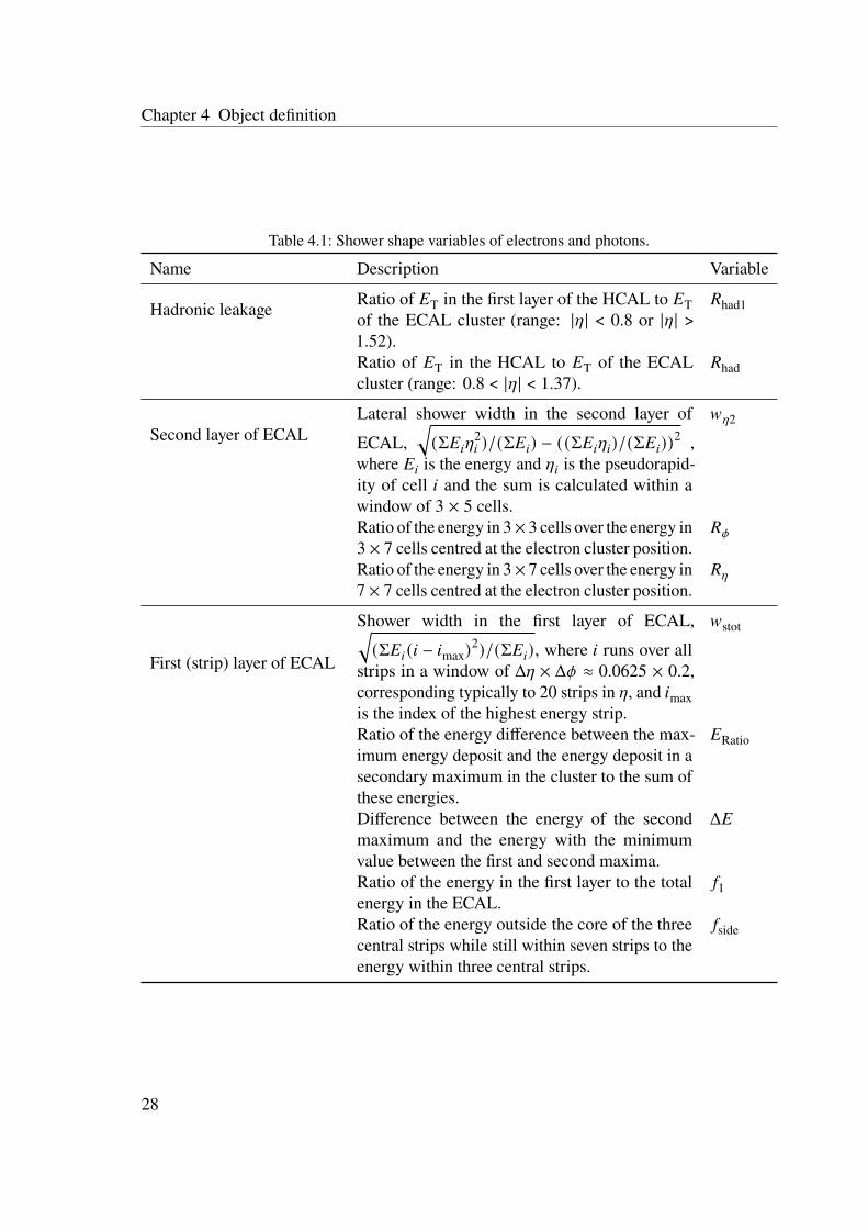
Table 4.1: Shower shape variables of electrons and photons.
Name Description Variable
Hadronic leakageRatio of �퐸T in the first layer of the HCAL to �퐸Tof the ECAL cluster (range: |�휂 | < 0.8 or |�휂 | >1.52).
�푅had1
Ratio of �퐸T in the HCAL to �퐸T of the ECALcluster (range: 0.8 < |�휂 | < 1.37).
�푅had
Second layer of ECALLateral shower width in the second layer of
ECAL,√
(Σ�퐸�푖�휂2�푖 )/(Σ�퐸�푖) − ((Σ�퐸�푖�휂�푖)/(Σ�퐸�푖))
2 ,where �퐸�푖 is the energy and �휂�푖 is the pseudorapid-ity of cell �푖 and the sum is calculated within awindow of 3 × 5 cells.
�푤�휂2
Ratio of the energy in 3× 3 cells over the energy in3 × 7 cells centred at the electron cluster position.
�푅�휙
Ratio of the energy in 3× 7 cells over the energy in7 × 7 cells centred at the electron cluster position.
�푅�휂
First (strip) layer of ECAL
Shower width in the first layer of ECAL,√
(Σ�퐸�푖 (�푖 − �푖max)2)/(Σ�퐸�푖), where �푖 runs over all
strips in a window of Δ�휂 × Δ�휙 ≈ 0.0625 × 0.2,corresponding typically to 20 strips in �휂, and �푖maxis the index of the highest energy strip.
�푤stot
Ratio of the energy difference between the max-imum energy deposit and the energy deposit in asecondary maximum in the cluster to the sum ofthese energies.
�퐸Ratio
Difference between the energy of the secondmaximum and the energy with the minimumvalue between the first and second maxima.
Δ�퐸
Ratio of the energy in the first layer to the totalenergy in the ECAL.
�푓1
Ratio of the energy outside the core of the threecentral strips while still within seven strips to theenergy within three central strips.
�푓side
28

4.2 Muons
energy loss in the calorimeter. These muon candidates expand the muons’ acceptanceto regions that are not covered by the ID (2.5 < |�휂 | < 2.7).
Since there is more than one type of muons, an overlap removal procedure is used toremove the duplication of muon candidates sharing the same ID track, which is done asfollows. CB muon candidates have the highest priority, followed by the segment-tagged,while the lowest priority is given to the calorimeter-tagged type. Furthermore, based on thegoodness of the fit and the number of hits, the overlap with the extrapolated muon candidatesis removed. In this work, only CB muons are considered since they have the highest purityand provide coverage of |�휂 | < 2.5.
Similar to electron candidates they are required to originate from the primary vertex, wherethe longitudinal impact parameter |�푧0 sin(�휃) | < 0.5 mm and transverse impact parameter�푑0 with significance |�푑0/�휎�푑0
| < 3. The candidates are also calibrated with the proceduredescribed in Ref. [61].
4.2.2 Identification and isolation
Muon identification criteria are needed to distinguish prompt muons from muons comingfrom hadron decays, mainly from pions and kaons decays. The various identification WPsare defined using different requirements on quantities, like the number of hits in the IDand/or the MS, the charge/momentum ratio between the ID and the MS tracks, and thegoodness of the combined-track fit. In this work, the Medium identification WP [61] is used,which has the advantage of having minimum systematic uncertainties during calibration andreconstruction. Similar to the isolation of electrons, the isolation of muons is also done byplacing requirements on track-based and calorimeter-based isolation variables. Here, theFCTight_FixedRad isolation WP is used, which requires that muons satisfy:
• �퐸topocone20T /�푝T(�휇) < 0.15 and
• for �푝T < 50 GeV : �푝varcone30T /�푝T(�휇) < 0.04 ,
for �푝T > 50 GeV : �푝cone20T /�푝T(�휇) < 0.04 ,
where �퐸topocone20T is a calorimeter-based isolation variable defined as the sum of energies
of topological clusters around the muon candidate excluding the energy of the muon itselfand �푝T(�휇) is the transverse momentum of the muon. Both of �푝
varcone30T and �푝
cone20T are
track-based isolation variables defined as the scalar sum of all tracks’ transverse momentawith a cone of Δ�푅 around the muon candidate, excluding the muon track itself where theformer uses a variable-radius cone of Δ�푅 = min (10 GeV/�푝T(�휇), 0.3) while the latter uses afixed-radius cone of Δ�푅 = 0.2.
29

Chapter 4 Object definition
4.3 Photons
4.3.1 Reconstruction
Photons and electrons produce similar signatures, in the form of electromagnetic showers,when interacting with the ECAL. Therefore, their reconstruction is performed in parallel.Photons are reconstructed using the same procedure as for electrons. Energy deposits inthe ECAL are clustered using a sliding-window algorithm. Then tracks are reconstructedin the ID and matched to the clusters in the ECAL to check if the candidate is a conver-ted/unconverted photon or simply an electron. If the ECAL clusters do not correspond toeither a conversion vertex or any track in the ID, then the candidate is reconstructed as anunconverted photon. However, if the ECAL clusters are matched to a conversion vertex, thecandidate is reconstructed as a converted photon. Both types, converted and unconvertedphotons, are considered in this work. Energies of the photon candidates are calibrated withthe procedure described in Ref. [62].
4.3.2 Identification and isolation
Photons in this work are identified using rectangular cuts on the shower shape variablesdescribed in Table 4.1. The identification of photons distinguishes between prompt photonsand background photons originating from decays of neutral hadrons (e.g. �휋
0 → �훾�훾) orQCD jets mimicking photons (jets deploying large energy fractions in the ECAL and aremis-reconstructed as photons). The distinction is performed based on the prompt photonsdepositing narrower energies in the ECAL and have smaller leakage to the HCAL comparedto background photons. Furthermore, non-prompt photons from �휋
0 → �훾�훾 decays arecharacterised by two separate local energy maxima in the first layer of the ECAL. There aretwo WPs for the identification of photons: Loose and Tight. The Loose identification is basedon the shower shapes in the second layer of the ECAL and on the energy deposits in theHCAL. The Tight identification makes use of the same info as in the Loose, but it adds to itadditional info from the finely segmented strip layer of the calorimeter. Since unconvertedand converted photons have slightly different shower shapes, the Tight identification criteriaare optimised separately for each of them. Moreover, due to the calorimeter geometry andthe effect on the shower shapes from different detector material, the identification WPs areoptimised as a function of the reconstructed photon candidate |�휂 |. In order to enhance thenumber of prompt photons, photons are required to be isolated. Isolation of photons is basedon the transverse energy in a cone of angular size Δ�푅 around the photon candidate. Suchtransverse energy depends on two quantities, calorimeter isolation and track isolation.
• �퐸isoT is the calorimeter isolation and is defined as the sum of transverse energies of
topological clusters [57] after subtracting the energy of the photon candidate and thecontribution from the underlying event and pile-up.
30

4.4 Jets
Table 4.2: Isolation WPs of photons.
WP Calorimeter isolation Track isolation
FixedCutLoose �퐸isoT
�
�
�
Δ�푅<0.2< 0.065 · �퐸T(�훾) �푝
isoT
�
�
�
Δ�푅<0.2< 0.05 · �퐸T(�훾)
FixedCutTight �퐸isoT
�
�
�
Δ�푅<0.4< 0.022 · �퐸T(�훾) + 2.45 GeV �푝
isoT
�
�
�
Δ�푅<0.2< 0.05 · �퐸T(�훾)
FixedCutTightCaloOnly �퐸isoT
�
�
�
Δ�푅<0.4< 0.022 · �퐸T(�훾) + 2.45 GeV –
• �푝isoT is the track isolation and is defined as the sum of transverse momenta of all the
tracks with transverse momentum above 1 GeV. Further requirements of having adistance to the primary vertex [52] along the beam axis |�푧0 sin �휃 | < 3 mm and exclusionof tracks associated with photon conversions must also be satisfied. In the ATLASCollaboration, there are three isolation WPs shown in Table 4.2. This work uses theWPs Tight for the identification and FixedCutTight for the isolation of photons.
4.3.3 Shower shapes reweighting
As already discussed earlier, shower shapes play a major role in the identification and isolationof photons. The simulation of the shower shapes in MC differs from the distributions in data.This could happen owing to a mis-modelling of the simulation or/and a leakage from thehadronic calorimeter, among other reasons. Therefore, a correction of the shower shapes isneeded so that the MC shapes match the data ones. A method to perform this correction isdescribed in Chapter 5.
4.4 Jets
4.4.1 Reconstruction
Quarks and gluons are colour-charged particles and, hence, they can not be observedexperimentally due to the colour confinement property of QCD. These partons hadronisevery quickly, forming a hadron which in turn decays to a collimated cascade of particlescollectively called a jet. Jets have associated tracks in the ID system and energy depositsin both the ECAL and HCAL systems. In order to reconstruct a jet, a clustering algorithmis needed to combine tracks in the ID system and energy deposits in the ECAL and HCALcalorimeters. Such an algorithm must be collinear and infrared safe. This means it mustensure that the jets are robust to collinear splittings and soft infrared radiations. In theATLAS Collaboration, the most commonly used algorithm is the anti-�푘�푡 algorithm [63]. Itis a sequential clustering algorithm that uses topological cell clusters [64] as inputs. Theseclusters are treated as massless pseudo-particles with four-momentum defined from the energy
31

Chapter 4 Object definition
Figure 4.1: Jet clustering example using the �푘�푡 (left) and anti-�푘�푡 (right) algorithms. The figures aresourced from Ref. [63].
and direction weighted by the barycentre of the cell cluster. The algorithm calculates twoparameters, the distance �푑�푖 �푗 between each pair of inputs, �푖 and �푗 , and the distance �푑�푖�퐵 betweeneach input �푖 and the beam axis as follows:
�푑�푖 �푗 = min(�푘2�푝
�푡,�푖, �푘
2�푝
�푡, �푗)Δ�푅
2�푖 �푗
�푅2
, (4.1a)
�푑�푖�퐵 = �푘2�푝
�푡,�푖, (4.1b)
where Δ�푅2�푖 �푗 = (�푦�푖 − �푦 �푗 )
2 − (�휙�푖 − �휙 �푗 )2 and �푘�푡 , �푦, and �휙 are the transverse momentum, rapidity,
and azimuthal angle of the input particle, respectively. �푅 is the radius parameter whichcontrols the approximate cone size of the final jet. The parameter �푝 determines the orderof the clustering where in the case of the anti-�푘�푡 algorithm, �푝 = −1, while in the case of �푘�푡algorithm [65], �푝 = 1. If �푝 is positive, then the algorithm will cluster particles from softest tohardest, while if it is negative, it behaves the other way around. The anti-�푘�푡 algorithm thenidentifies the smallest distance, which is the minimum of �푑�푖 �푗 and �푑�푖�퐵. If the smallest distanceis �푑�푖 �푗 , then clusters �푖 and �푗 are combined. If �푑�푖�퐵 is the smallest, then �푖 is called a jet andremoved from the list of clusters. This process is repeated for all the topological clusters untilno clusters are left in the list. The anti-�푘�푡 algorithm results in more cone-like jets comparedto clusters combined with the �푘�푡 algorithm which can be seen in Fig. 4.1.
In this work, jets are reconstructed using the anti-�푘�푡 algorithm in the FastJet implementa-tion [66] with a radius parameter �푅 = 0.4.
4.4.2 Calibration
Once jets are reconstructed, calibration techniques are used to calibrate their four-momentain the MC simulation and data. In general, there are two methods used in combination: MC-based and in-situ techniques. The former is to correct the four-momenta of the reconstructedjet to the particle-level truth jet, while the latter is to correct for the differences in jet response
32

4.4 Jets
Figure 4.2: A schematic overview of the jet calibration steps in the ATLAS detector. The figure issourced from Ref. [67].
between data and MC. The calibration of jets is divided into several steps, as shown inFig. 4.2. First, the origin of the jet is corrected so that it points to the primary vertex ratherthan the centre of the detector, which improves the resolution in �휂. Next, the excess inenergy originating from the in-time and out-of-time pile-up is removed. In-time (out-of-time)pile-up is defined as additional �푝�푝 interactions from the same (neighbouring) bunch crossings.This correction is done by subtracting the per-event pile-up contribution to the �푝T of eachjet according to its area, hence an area-based correction. After this pile-up correction, adependency of the anti-�푘�푡 jet �푝T on the amount of pile-up remains. Therefore, a furthercorrection is applied, which is called residual pile-up correction. After pile-up corrections,an MC-based calibration is used. It uses the absolute jet energy scale (JES) and �휂-calibrationto correct the four-momentum of the reconstructed jet to the particle-level true energy scaleand account for biases in the jet-�휂 reconstruction. The next step is called the global sequentialcalibration. It removes the residual dependencies due to differences in the composition ofquark- and gluon-initiated jets and accounts for energy leakage effects. The last step in the jetcalibration is called residual in-situ. It accounts for differences in the jet response betweendata and MC due to the mis-modelling of the detector response and detector material in theMC simulation.
4.4.3 �풃-tagging
The distinction between jets originating from hadrons with �푏-quarks, so-called �푏-jets, andjets from hadrons with other quark flavours is essential for analyses studying properties ofthe top quark, such as the one presented here. A property of hadrons with �푏-quarks, called�푏-hadrons, is that they have a much longer lifetime than light-flavour hadrons and hencetravel for a measurable distance before they decay. Light-flavour hadrons are hadrons with �푢-,�푑- or �푠- quarks. Therefore, �푏-hadrons can be identified by the presence of a secondary vertexdisplaced from the primary vertex of the hard interaction. Furthermore, they are heavier and
33

Chapter 4 Object definition
produce more energetic decay products compared to the light-flavour hadrons. In the ATLASCollaboration, a very common �푏-tagging algorithm is the MV2c10 [68]. It is a multivariatediscriminant algorithm that distinguishes between different jet flavours and uses as input thefollowing �푏-tagging algorithms:
• IP2D and IP3D impact parameter algorithms [69] are techniques that use the transverseand longitudinal track impact parameters of the tracks associated with �푏-hadron decaysto identify the �푏-hadrons. The outcome of such algorithms is a log-likelihood ratio forthe possible combinations of different jet flavours.3
• Secondary vertex SV1 [70] is an algorithm that reconstructs a single displaced secondaryvertex inside a jet. The reconstruction is performed by checking all possible two-trackvertices and rejecting tracks in agreement with the decay of long-lived particles.
• JetFitter [71] performs a topological reconstruction of the �푏-hadron decays inside thejet. The algorithm is of high importance when a higher level of �푐- and light jet rejectionis needed while maintaining an intermediate �푏-jet efficiency.
In this work, the MV2c10 [68] algorithm is used with a WP of 85% �푏-tagging efficiency,which corresponds to �푐- and light-jet rejection factors of 3.1 and 35, respectively.
4.5 Missing transverse energy
Some particles escape the ATLAS detector without any detection, i.e. they do not leavetracks in the ID and do not deposit energies in the calorimeters. These invisible particles areneutrinos in the case of the SM. They can also hint to other hypothetical weakly-interactingparticles in the case of theories beyond the SM. Their presence is detected indirectly owingto the energy and momentum conservation in the transverse plane, and it is quantified as the
missing energy−→�퐸
miss�푇 . It is defined as the magnitude of �푝miss
T with an azimuthal coordinate of
�휙miss. The
−→�퐸
miss�푇 comprises two terms where the first one depends on the different objects
(electrons, muons, photons, jets and the hadronically-decaying �휏-leptons that come from theprimary interaction, i.e. hard objects) in an event, and therefore they need to be well-calibratedand reconstructed [72]. The second term is called the soft term, which depends on tracks inthe ID system or calorimeter energy deposits that are not associated with physics objects (soft
signals). The first term has a slight dependence on pile-up since it depends on well-calibratedobjects where the pile-up contribution is already accounted for and corrected. However,the second term is not robust against pile-up and therefore further techniques are used to
correct it. The−→�퐸
miss�푇 has two components �퐸miss
�푥 and �퐸miss�푦 , which are expressed in the �푥- and
�푦-components of the �푝missT , �푝miss
�푥(�푦) :
3 The combinations are �푏- and light jet, �푏- and �푐-jet, and �푐- and light jet, where light jet is a jet with �푢-, �푑- or �푠-quarks.
34

4.5 Missing transverse energy
�퐸miss�푥(�푦) = −
∑
all hard objects
�푝miss�푥(�푦) −
∑
all soft signals
�푝miss�푥(�푦) , (4.2)
from which the �퐸miss�푇 is calculated as:
�퐸miss�푇 =
√
(�퐸miss�푥 )2 + (�퐸miss
�푦 )2. (4.3)
35

CHAPTER 5
Shower shapes reweighting for photons
The photon shower shapes differ between MC and data due to mis-modelling of the simulationand/or leakage from the hadronic calorimeter. The motivation for the study in this chapter isto improve the agreement between data and MC shower shapes (for definitions of showershapes, see Table 4.1) by applying a correction to the MC shapes using a cell-based energyreweighting of the photons. After applying the correction, the MC shower shapes of thephotons would better mimic those in the data.
In this chapter, the data and MC samples used in the shower shapes reweighting arepresented in Section 5.1. The method of cell-based reweighting of photons is introducedin Section 5.2. The applied event selection and the approaches to obtain a pure sample aredescribed in Sections 5.3 and 5.4, respectively. Results of the study are presented at the endof the chapter in Section 5.5.
5.1 Data and MC samples
This study is performed with �푝�푝 collision data collected during the years 2 015, 2 016, and2 017 at
√�푠 = 13 TeV, with the corresponding integrated luminosities of 3.2 fb
−1, 33.0 fb−1,
and 44.3 fb−1, respectively. The total collision data correspond to an integrated luminosity
of 80.5 fb−1 and are required to have been collected while the ATLAS detector was fully
operational and satisfied quality criteria. The �푍 → �푒�푒�훾 MC samples used for this study aregenerated with Sherpa 2.2.2 using the NNPDF3.0NNLO [73] and CT10 [74] PDF sets.
5.2 Cell-based energy reweighting of photons
The correction of the shower shape variables of photons is performed through a reweightingto the cell-based energies of photons along the �휂-direction. In order to derive such correction,photons are matched to clusters in the second layer of the ECAL with different sizes ofclusters in the �휂-�휙 space. More specifically, photons are matched to clusters with �휂 × �휙 cells
37

Chapter 5 Shower shapes reweighting for photons
of sizes 3 × 7 in the barrel and 5 × 5 in the end-cap regions. In addition, a matching ofphotons to a bigger-size cluster of 7 × 11 is also constructed which surrounds the 3 × 7 and5 × 5 clusters. The reason behind the construction of the bigger cluster is to study the lateralenergy leakage. To construct the 7 × 11 cluster, two steps are needed:
• Firstly, the central cell of the cluster has to be located. The closest cell with the minimalΔ�푅 around the photon cluster which passes the selection is stored. Next, within aΔ�푅 < 0.5 around the located cell, a search for the cell with the largest energy depositis performed; as a result, such cell with the maximum energy is considered to be thecentral cell of the cluster.
• Secondly, the construction of 7 × 11 cluster around the central cell is performed.Important information like energies, �휂 and �휙 are stored for the 77 cells; only a completenumber of 77 cells are kept.
Once the 7 × 11 cluster is built, the weights (to correct the MC simulation) are calculatedas ratios of the data energy per cell to the MC one along �휂-direction, �퐸data
�푖 /�퐸MC�푖 , where �푖 is
the index of the cell.
5.3 Event selection
The cell-based energy reweighting is studied by investigating photons originating from theradiative decay process of the �푍 boson, i.e. �푍 → �푒�푒�훾. Such a process has the advantageof having a relatively small fraction of backgrounds. The primary source of backgroundis due to photons originating from jets mimicking photons (from �푍+jets). The selection isapplied such that events are required to include at least one primary vertex with at least threeassociated tracks, an electron-positron pair, and one photon. Photons and electrons mustfulfil the criteria described in Table 5.1. Furthermore, a requirement on the mass of theelectron-positron pair is placed: 40 < �푚�푒�푒 < 83 GeV. Despite the object and event selectionrequirements, there still exists a large portion of background, as shown in the �푚�푒�푒�훾 distributionin Fig. 5.1. Therefore, additional approaches are needed to select a pure �푍 → �푒�푒�훾 sample, asdiscussed in the following section.
5.4 Pure �풁 → �풆�풆�휸 sample
In order to study the effect of the cell reweighting on the shower shapes of prompt photons,it is necessary to have a pure �푍 → �푒�푒�훾 sample. The aim is to remove the backgroundcontamination in data, mainly in the peak region of the �푚�푒�푒�훾 distribution (see Fig. 5.1). Afterapplying the selection in Section 5.3, the remaining background contribution is accountedfor by a reweighting based on the signal fraction or by tightening the selection requirements.Therefore, two approaches are tested where the first one is used as the benchmark, whereasthe second is used as a verification:
38

5.4 Pure �푍 → �푒�푒�훾 sample
Table 5.1: Object definition of electrons and photons for the cell-based energy reweighting ofphotons. The MediumLH identification WP has an efficiency of 88% for selecting a promptelectron with �퐸T = 40 GeV. The GradientLoose isolation WP has an isolation efficiency of95 (99)% at 25 (60) GeV [57].
Electrons Photons
Acceptance
�푝T > 10 GeV �퐸T > 10 GeV|�휂 | < 1.37 , 1.52 < |�휂 | < 2.47 |�휂 | < 1.37, 1.52 < |�휂 | < 2.37
|�푑0 / �휎�푑0| < 10 —
|�푧0 sin(�휃) | < 10 mm —
Identification MediumLH —
Isolation GradientLoose —
• The first approach is based on a signal fraction reweighting. This is performed byfitting the �푚�푒�푒�훾 distribution in data, followed by a window cut of 80 < �푚�푒�푒�훾 < 100 GeV.The fit function is a combination of a Crystal-ball function (for signal) and fourth-orderBernstein polynomial (for background). The fit is performed for each of the measured�푍 → �푒�푒�훾 datasets (2015–2017) independently. An example of the fit for the dataset ofthe year 2017 can be seen in Fig. 5.2. The fits for the datasets corresponding to 2015and 2016 can be seen in Appendix A. Afterwards, from the post-fit results a signalfraction weight �푊sf is estimated in each bin of the �푚�푒�푒�훾:
�푊sf =signal
signal + background. (5.1)
These weights are then applied to the shower shapes of data to correct for the backgroundcontamination. An example of the weights calculated from the fit to the 2017 datasetcan be seen in Fig. 5.3. The weights corresponding to the datasets of the years 2015and 2016 can be found in Appendix A.
• Additionally, a second approach is used to verify the first one, by applying a photonisolation WP FixedCutLoose
1 , followed by a window cut of 80 < �푚�푒�푒�훾 < 100 GeV.
The two approaches are compared to the nominal case where the latter represents applyingonly the event selection (see Section 5.3) without any further requirements to reduce thebackground. The results of the two approaches in the inclusive �휂 region for converted andunconverted photons are discussed in Section 5.5.1. The results of the cell reweightingcorrection are shown in Section 5.5.2.
1 This WP is chosen as loose as possible to avoid causing a bias in the shower shapes, which are intended to becorrected in the first place.
39

Chapter 5 Shower shapes reweighting for photons
0
10000
20000
30000
40000
50000
60000
Eve
nts
γInclusive
-1=13 TeV, 80.5 fbs Data
MCγ ee→ Z
0 20 40 60 80 100 120 140 160 180 200
[GeV]γeem
0.5
1
1.5
Da
ta/M
C
Figure 5.1: Invariant mass distribution of �푚�푒�푒�훾 in data (black) and MC (red) in the inclusive �휂 region:0 < |�휂(�훾) | < 1.37 or 1.52 < |�휂(�훾) | < 2.37 for inclusive (converted and unconverted) photons.
40

5.4 Pure �푍 → �푒�푒�훾 sample
50 60 70 80 90 100 110 120 [GeV]γeem
0
5000
10000
15000
20000
25000
30000
Events
/ 1
GeV
Data
Signal+Background
Signal
Background
-1=13 TeV, 44.3 fbs
γInclusive
Figure 5.2: Example of the fit to the �푚�푒�푒�훾 distribution of �푍 → �푒�푒�훾 data for the year 2017, where aCrystal-ball function and 4th order Bernstein polynomial are used to model signal and background,respectively.
50 60 70 80 90 100 110 120 [GeV]γeem
0.2
0.3
0.4
0.5
0.6
0.7
0.8
0.9
sf
W
-1=13 TeV, 44.3 fbs
γInclusive
Figure 5.3: Example of signal fraction weights �푊sf, calculated from the post-fit results of the �푍 → �푒�푒�훾
data for the year 2017 using Eq. (5.1).
41

Chapter 5 Shower shapes reweighting for photons
5.5 Results of cell-based reweighting
5.5.1 Background reduction
Fig. 5.4 shows the �푚�푒�푒�훾 distribution in the data and the MC simulation for converted (leftcolumn) and unconverted (right column) photons. The first row displays the data distributionswithout applying any additional requirements beyond the selection in Section 5.3. The secondand third rows show the data distributions after applying the first and second approaches,respectively. The behaviour of the two approaches is similar, where most of the backgroundcontribution is removed. The first approach is chosen as the benchmark for all the results inthe main body of the thesis, while the results of the second approach and more studies, suchas showing the distributions in different slices of �휂, can be found in Appendix A.
5.5.2 Cell-based energy reweighting
As an example, in the case of �푅�휂 distribution, the top and bottom plots of Fig. 5.5 show themodelling of the shower shape for converted and unconverted photons, respectively. The datadistributions to the right have the first approach applied to them, whereas the data distributionsto the left do not have any requirements beyond the event selection. The shapes of the data inthe left column look similar to those of the right, indicating no bias due to the first approachbackground reduction. This can be seen for the rest of the shower shapes as well.
In order to examine the impact of the cell-based reweighting correction, the MC showershapes before and after correction are compared to those of the data , which can be seen, forexample, for �푅�휂 in the right plots of Fig. 5.5. The correction for �푅�휂 gives a better agreementwith data for both converted and unconverted photons. For �푅�휙, the correction, in general, doesnot improve the agreement significantly, as can be seen in Fig. 5.6. For �푅had, �푓1, �퐸Ratio andΔ�퐸 , they are similar to �푅�휙, and are shown in Appendix A. The correction for �푤�휂2 provides abetter agreement with data, as shown in Fig. 5.7. The improvement for converted photonsis more enhanced than the unconverted photons. For �푤stot, the correction gives a moderateimprovement at the lower and higher tails of both converted and unconverted photonsdistributions, as shown in Fig. 5.8. For �푓side, the correction gives a noticeable improvementin the case of converted photons as can been seen in Fig. 5.9, while for unconverted photons,the correction slightly improves the agreement with data.
In summary, the results of the cell-based energy reweighting of photons show a goodimprovement in the agreement between data and MC shower shapes, especially for the �푅�휂,�푤�휂2, �푤stot and �푓side shower shapes. However, for the rest of the shower shapes, i.e., �푅�휙, �푅had1,�푓1, �퐸Ratio and Δ�퐸 , the correction does not improve the data/MC agreement significantly.
42

5.5 Results of cell-based reweighting
0
2000
4000
6000
8000
10000
12000
14000
16000
18000
20000
Eve
nts
γConverted
-1=13 TeV, 80.5 fbs Data
MCγ ee→ Z
0 20 40 60 80 100 120 140 160 180 200
[GeV]γeem
0.5
1
1.5
Da
ta/M
C
0
10000
20000
30000
40000
50000
60000
Eve
nts
γUnconverted
-1=13 TeV, 80.5 fbs Data
MCγ ee→ Z
0 20 40 60 80 100 120 140 160 180 200
[GeV]γeem
0.5
1
1.5
Da
ta/M
C
0
2000
4000
6000
8000
10000
12000
14000
16000
18000
20000
Eve
nts
γConverted
-1=13 TeV, 80.5 fbs
1st approach
Data - Bkg.
MCγ ee→ Z
70 75 80 85 90 95 100 105 110
[GeV]γeem
0.5
1
1.5
Data
/MC
0
10000
20000
30000
40000
50000
60000
Eve
nts
γUnconverted
-1=13 TeV, 80.5 fbs
1st approach
Data - Bkg.
MCγ ee→ Z
70 75 80 85 90 95 100 105 110
[GeV]γeem
0.5
1
1.5
Data
/MC
0
2000
4000
6000
8000
10000
12000
14000
16000
18000
20000
Eve
nts
γConverted
-1=13 TeV, 80.5 fbs
2nd approach
Data - Bkg.
MCγ ee→ Z
70 75 80 85 90 95 100 105 110
[GeV]γeem
0.5
1
1.5
Data
/MC
0
10000
20000
30000
40000
50000
60000
Eve
nts
γUnconverted
-1=13 TeV, 80.5 fbs
2nd approach
Data - Bkg.
MCγ ee→ Z
70 75 80 85 90 95 100 105 110
[GeV]γeem
0.5
1
1.5
Data
/MC
Figure 5.4: Invariant mass distributions of �푚�푒�푒�훾 in data (black) and MC (red) in the inclusive �휂 region:0 < |�휂(�훾) | < 1.37 or 1.52 < |�휂(�훾) | < 2.37. The left (right) column shows for converted (unconverted)photons, three distributions: nominal event selection case (top), first approach (middle), and secondapproach (bottom). In the middle and bottom rows, the background contribution in �푍 → �푒�푒�훾 data hasbeen further reduced using either the first or second approach, respectively, while in the top row, norequirements are added beyond the event selection described in Section 5.3. 43

Chapter 5 Shower shapes reweighting for photons
0
0.02
0.04
0.06
0.08
0.1
0.12
0.14
A. U
.
γConverted
-1=13 TeV, 80.5 fbs Data
MCγ ee→ Z MC Correctedγ ee→ Z
0.9 0.92 0.94 0.96 0.98 1
ηR
1
2
Data
/MC
0
0.02
0.04
0.06
0.08
0.1
0.12
0.14
A. U
.
γConverted
-1=13 TeV, 80.5 fbs
1st approach
Data - Bkg. MCγ ee→ Z MC Correctedγ ee→ Z
0.9 0.92 0.94 0.96 0.98 1
ηR
1
1.5D
ata
/MC
0
0.02
0.04
0.06
0.08
0.1
0.12
0.14
A. U
.
γUnconverted
-1=13 TeV, 80.5 fbs Data
MCγ ee→ Z MC Correctedγ ee→ Z
0.9 0.92 0.94 0.96 0.98 1
ηR
1
2
Data
/MC
0
0.02
0.04
0.06
0.08
0.1
0.12
0.14
A. U
.
γUnconverted
-1=13 TeV, 80.5 fbs
1st approach
Data - Bkg. MCγ ee→ Z MC Correctedγ ee→ Z
0.9 0.92 0.94 0.96 0.98 1
ηR
1
1.5
Data
/MC
Figure 5.5: �푅�휂 distributions in data (black) and MC before (red) and after (blue) cell-based correctionin the inclusive �휂 region: 0 < |�휂(�훾) | < 1.37 or 1.52 < |�휂(�훾) | < 2.37. In the top (bottom) row forconverted (unconverted) photons, two distributions are shown: nominal event selection case (left) andfirst approach (right).
44
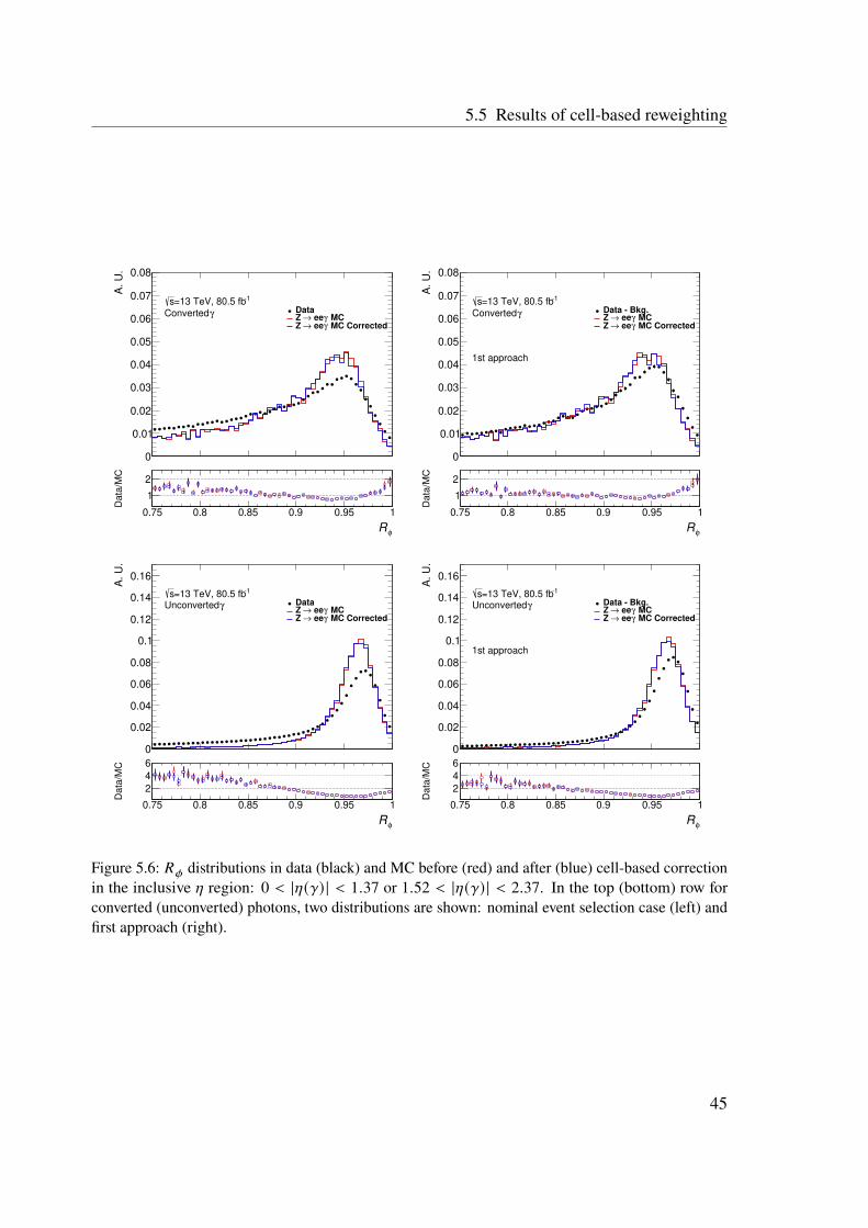
5.5 Results of cell-based reweighting
0
0.01
0.02
0.03
0.04
0.05
0.06
0.07
0.08
A. U
.
γConverted
-1=13 TeV, 80.5 fbs Data
MCγ ee→ Z MC Correctedγ ee→ Z
0.75 0.8 0.85 0.9 0.95 1
φR
1
2
Data
/MC
0
0.01
0.02
0.03
0.04
0.05
0.06
0.07
0.08
A. U
.
γConverted
-1=13 TeV, 80.5 fbs
1st approach
Data - Bkg. MCγ ee→ Z MC Correctedγ ee→ Z
0.75 0.8 0.85 0.9 0.95 1
φR
1
2
Data
/MC
0
0.02
0.04
0.06
0.08
0.1
0.12
0.14
0.16
A. U
.
γUnconverted
-1=13 TeV, 80.5 fbs Data
MCγ ee→ Z MC Correctedγ ee→ Z
0.75 0.8 0.85 0.9 0.95 1
φR
2
4
6
Data
/MC
0
0.02
0.04
0.06
0.08
0.1
0.12
0.14
0.16
A. U
.
γUnconverted
-1=13 TeV, 80.5 fbs
1st approach
Data - Bkg. MCγ ee→ Z MC Correctedγ ee→ Z
0.75 0.8 0.85 0.9 0.95 1
φR
2
4
6
Data
/MC
Figure 5.6: �푅�휙 distributions in data (black) and MC before (red) and after (blue) cell-based correctionin the inclusive �휂 region: 0 < |�휂(�훾) | < 1.37 or 1.52 < |�휂(�훾) | < 2.37. In the top (bottom) row forconverted (unconverted) photons, two distributions are shown: nominal event selection case (left) andfirst approach (right).
45

Chapter 5 Shower shapes reweighting for photons
0
0.02
0.04
0.06
0.08
0.1
0.12A. U
.
γConverted
-1=13 TeV, 80.5 fbs Data
MCγ ee→ Z MC Correctedγ ee→ Z
0.008 0.009 0.01 0.011 0.012 0.013
2ηw
0
2
Data
/MC
0
0.02
0.04
0.06
0.08
0.1
0.12A. U
.
γConverted
-1=13 TeV, 80.5 fbs
1st approach
Data - Bkg. MCγ ee→ Z MC Correctedγ ee→ Z
0.008 0.009 0.01 0.011 0.012 0.013
2ηw
0
2D
ata
/MC
0
0.02
0.04
0.06
0.08
0.1
0.12
0.14
A. U
.
γUnconverted
-1=13 TeV, 80.5 fbs Data
MCγ ee→ Z MC Correctedγ ee→ Z
0.008 0.009 0.01 0.011 0.012 0.013
2ηw
0
2
4
Data
/MC
0
0.02
0.04
0.06
0.08
0.1
0.12
0.14
A. U
.
γUnconverted
-1=13 TeV, 80.5 fbs
1st approach
Data - Bkg. MCγ ee→ Z MC Correctedγ ee→ Z
0.008 0.009 0.01 0.011 0.012 0.013
2ηw
0
2
4
Data
/MC
Figure 5.7: �푤�휂2 distributions in data (black) and MC before (red) and after (blue) cell-based correctionin the inclusive �휂 region: 0 < |�휂(�훾) | < 1.37 or 1.52 < |�휂(�훾) | < 2.37. In the top (bottom) row forconverted (unconverted) photons, two distributions are shown: nominal event selection case (left) andfirst approach (right).
46

5.5 Results of cell-based reweighting
0
0.02
0.04
0.06
0.08
0.1
0.12A. U
.
γConverted
-1=13 TeV, 80.5 fbs Data
MCγ ee→ Z MC Correctedγ ee→ Z
0.5 1 1.5 2 2.5 3 3.5 4
stotw
0
2
4
Data
/MC
0
0.02
0.04
0.06
0.08
0.1
0.12A. U
.
γConverted
-1=13 TeV, 80.5 fbs
1st approach
Data - Bkg. MCγ ee→ Z MC Correctedγ ee→ Z
0.5 1 1.5 2 2.5 3 3.5 4
stotw
0
2
4
Data
/MC
0
0.02
0.04
0.06
0.08
0.1
0.12
0.14
0.16
A. U
.
γUnconverted
-1=13 TeV, 80.5 fbs Data
MCγ ee→ Z MC Correctedγ ee→ Z
0.5 1 1.5 2 2.5 3 3.5 4
stotw
0
2
4
Data
/MC
0
0.02
0.04
0.06
0.08
0.1
0.12
0.14
0.16
A. U
.
γUnconverted
-1=13 TeV, 80.5 fbs
1st approach
Data - Bkg. MCγ ee→ Z MC Correctedγ ee→ Z
0.5 1 1.5 2 2.5 3 3.5 4
stotw
0
2
4
Data
/MC
Figure 5.8: �푤stot distributions in data (black) and MC before (red) and after (blue) cell-based correctionin the inclusive �휂 region: 0 < |�휂(�훾) | < 1.37 or 1.52 < |�휂(�훾) | < 2.37. In the top (bottom) row forconverted (unconverted) photons, two distributions are shown: nominal event selection case (left) andfirst approach (right).
47

Chapter 5 Shower shapes reweighting for photons
0
0.05
0.1
0.15
0.2
0.25
0.3
0.35
0.4
0.45
A. U
.
γConverted
-1=13 TeV, 80.5 fbs Data
MCγ ee→ Z MC Correctedγ ee→ Z
0 0.1 0.2 0.3 0.4 0.5 0.6 0.7 0.8 0.9 1
sidef
0
2
4
6
Data
/MC
0
0.05
0.1
0.15
0.2
0.25
0.3
0.35
0.4
0.45
A. U
.
γConverted
-1=13 TeV, 80.5 fbs
1st approach
Data - Bkg. MCγ ee→ Z MC Correctedγ ee→ Z
0 0.1 0.2 0.3 0.4 0.5 0.6 0.7 0.8 0.9 1
sidef
0
2
4
6D
ata
/MC
0
0.1
0.2
0.3
0.4
0.5
A. U
.
γUnconverted
-1=13 TeV, 80.5 fbs Data
MCγ ee→ Z MC Correctedγ ee→ Z
0 0.1 0.2 0.3 0.4 0.5 0.6 0.7 0.8 0.9 1
sidef
0246
Data
/MC
0
0.1
0.2
0.3
0.4
0.5
A. U
.
γUnconverted
-1=13 TeV, 80.5 fbs
1st approach
Data - Bkg. MCγ ee→ Z MC Correctedγ ee→ Z
0 0.1 0.2 0.3 0.4 0.5 0.6 0.7 0.8 0.9 1
sidef
0246
Data
/MC
Figure 5.9: �푓side distributions in data (black) and MC before (red) and after (blue) cell-based correctionin the inclusive �휂 region: 0 < |�휂(�훾) | < 1.37 or 1.52 < |�휂(�훾) | < 2.37. In the top (bottom) row forconverted (unconverted) photons, two distributions are shown: nominal event selection case (left) andfirst approach (right).
48

CHAPTER 6
Data and MC simulation for �풕 �풕�휸 + �풕�푾�휸
measurement
In this thesis, the fiducial differential cross-section of the combined �푡�푡�훾 and �푡�푊�훾 process inthe �푒�휇 decay channel is measured. The signature of signal events can be mimicked by otherphysics processes, which are called background processes. Therefore, MC simulations arecompared to data to determine the composition of signal and background processes.
In this chapter, the data used to perform the measurement is discussed in Section 6.1. Asummary of steps to generate an MC simulation is discussed in Section 6.2. The simulationof signal and background processes is discussed in Section 6.3 and Section 6.4, respectively.The method of overlap removal between the samples is illustrated in Section 6.5.
6.1 Data
The measurements presented here are performed with data collected by the ATLAS detectorduring Run 2 of the LHC in the period of 2 015–2 018 at
√�푠 = 13 TeV. A subset of the total
collected data is considered good if the detector was fully operational and the recorded datasatisfied certain quality criteria. These data correspond to integrated luminosities of 3.2,33.0, 44.3, and 58.5 fb
−1 for the the years 2 015 to 2 018, respectively, i.e. a total integratedluminosity of 139 fb
−1. The mean number of interactions per bunch crossing (pile-up) for thedata recorded in the years 2 015–2 018 with the ATLAS detector is shown in Fig. 6.1.
6.2 MC simulation
MC simulations are needed to estimate the contribution of different physics processes inthe measured data. They are also used to evaluate efficiencies, migration, and acceptance,which are discussed in Chapter 8. Furthermore, they are used to account for the in-timeand out-of-time pile-up by superimposing hard-scattering (discussed below) events with
49

Chapter 6 Data and MC simulation for �푡�푡�훾 + �푡�푊�훾 measurement
0 10 20 30 40 50 60 70 80
Mean Number of Interactions per Crossing
0
100
200
300
400
500
600/0
.1]
-1R
ecord
ed L
um
inosity [pb
Online, 13 TeVATLAS-1Ldt=146.9 fb∫
> = 13.4µ2015: <
> = 25.1µ2016: <
> = 37.8µ2017: <
> = 36.1µ2018: <
> = 33.7µTotal: <
2/1
9 c
alib
ratio
n
Figure 6.1: Pile-up distributions for the data recorded by the ATLAS experiment in the years2 015–2 018. The figure is sourced from Ref. [75].
minimum-bias interactions generated with Pythia 8 [76]. The MC simulations are producedthrough different steps: event generation, detector simulation and digitisation of the depositedenergy. The final output of these simulations can then be run through the ATLAS trigger andreconstruction algorithms to compare the corresponding objects in the measurement and thesimulation.
Event generation
The first step is to generate events mimicking the production rate and kinematic properties ofthe processes under study. This step is called event generation, and it comprises differentconsequent processes; the first one is called hard scattering. The Matrix Element (ME)calculation of the hard scattering process is performed in the perturbation theory at fixedorder. In the hard scattering, collisions of protons are simulated where the PDF determinesthe probability that the partons in the protons collide.
Next is the showering process, which simulates the radiation of gluons and photons, calledQCD and QED radiations, respectively. These radiations are called Initial State Radiation
50

6.3 Simulation of signal
(ISR) if they come from the incoming partons and Final State Radiation (FSR) if comingfrom the outgoing particles. The simulation of such radiations is a complex process becausepartons radiate gluons, which can, in turn, emit further gluons—since gluons carry color—orproduce �푞�푞 pairs. This leads to the formation of a cascade of particles called the parton
shower.The last step in the event generation is the hadronisation process, where partons form
hadrons and decay to stable particles. Hadronisation occurs due to the confinement propertyof QCD (see Section 2.1).
Detector simulation and digitisation
Once events are generated, they are fed to the second step which is the detector simulation.The full simulation of the ATLAS detector is done using the Geant4 [77–79] by modellingthe physics of the traversing particles and their interactions (hits) through their trajectories inthe different systems of ATLAS. Such simulation is continuously updated so that it becomesfaster and more accurate. Furthermore, to estimate some of the modelling uncertainties, afast simulation known as AtlFast-II [79, 80] is employed to avoid the intensive computationneeded for the full simulation.
6.3 Simulation of signal
This thesis aims to compare the measurement with the NLO theory prediction of the process�푝�푝 → �푏ℓ�휈�푏ℓ�휈�훾 in the �푒�휇 channel [9]. It was not feasible to simulate this 2 → 7 process, sothe signal process is instead simulated as the combination of the double-resonant �푡�푡�훾 andsingle-resonant �푡�푊�훾.
Double-resonant �풕 �풕�휸
The �푡�푡�훾 process is simulated as a 2 → 7 process with the MadGraph5_aMC@NLO generator[81] and the NNPDF2.3LO PDF set where the ME is at LO accuracy in QCD including thedecay of the top quarks and using a filter to produce final states with at least one chargedlepton. The events are generated for the process �푝�푝 → �푏�푙�휈�푏�푙�휈�훾 where the photon is radiatedoff the incoming charged partons (ISR radiations from the �푞�푞 annihilation), intermediate topquarks, �푏-quarks, intermediate �푊 bosons, or the charged decay products of the intermediate�푊 bosons. To ensure infrared and collinear safety, photons are required to have �푝T > 15 GeV
and |�휂 | < 5.0 and leptons to have |�휂 | < 5.0. Furthermore, the photons are ensured to beisolated where a Δ�푅 > 0.2 between the photon and any charged lepton of the seven final-stateparticles is kept. The top-quark mass is set to 172.5 GeV in this and all other samples,including top quarks. The renormalisation �휇R and factorisation �휇F scales are chosen to bedynamic and are calculated as
51
Chapter 6 Data and MC simulation for �푡�푡�훾 + �푡�푊�훾 measurement
�휇R = �휇F =1
2× Σ�푖
√
�푚2�푖 + �푝
2T,�푖 , (6.1)
where �푚�푖 and �푝T,�푖 are the mass and transverse momentum of particle �푖, respectively, where�푖 runs over all particles generated from the ME calculation. In order to model the partonshowers, the hadronisation, the fragmentation, and the underlying event, the event generationis interfaced to Pythia 8 (v8.212) with the A14 [76] parameter tune. The EvtGen [82] isemployed to model the heavy-flavour hadron decays.
Single-resonant �풕�푾�휸
The �푡�푊�훾 process is simulated with two complementary samples generated with the Mad-
Graph5_aMC@NLO generator at LO in QCD and the NNPDF2.3LO PDF set. The firstsample simulates the �푝�푝 → �푡�푊�훾 process in the five-flavour scheme while assuming the topquark to be stable. In the five-flavour scheme, the �푏-quarks are treated as massless wherethey are assumed to be in the initial state, meaning that they are considered partons in theprotons. This simplifies and gives a more accurate calculation compared to the four-flavourscheme. The first sample includes photons radiated during the production of the top quarkand the �푊 boson or radiated from the initial state particles. The second sample simulatesthe �푝�푝 → �푏�푊�푏�푊�훾 process in the five-flavour scheme where the photon is radiated fromany other charged final-state particle. The two samples are complementary since the firstone simulates the radiation of photons during production while the second simulates thephotons during decay, which are combined to give the full simulation of the �푡�푊�훾 process.Similar to the �푡�푡�훾 sample, both �푡�푊�훾 samples are interfaced with Pythia 8 (v8.212) for partonshowering using the A14 tune and use EvtGen to model the heavy-flavour hadron decays.Also similarly to the �푡�푡�훾 sample, photons are required to have �푝T > 15 GeV and photons andleptons are required to have |�휂 | < 5.0. Furthermore, a Δ�푅 > 0.2 between the photon and anycharged lepton of the seven final-state particles is maintained.
6.4 Simulation of background processes
The background events come from different processes, which are simulated using the samplesenlisted below.
(�푾�휸/�풁�휸) + jets
The �푊�훾+jets and �푍�훾+jets processes are generated using different versions of the Sherpa
generator [83, 84]. The�푊�훾+jets events are generated with the Sherpa 2.2.4 at NLO accuracyin QCD using the NNPDF3.0NNLO PDF set, and the �푍�훾+jets events are generated withSherpa 2.2.4 using the same PDF set. All �푊�훾+jets/�푍�훾+jets events are normalised to the
52

6.4 Simulation of background processes
cross-sections of the corresponding MC simulation. The Sherpa generator simulates all theevent generation steps, from the hard scattering to the final observable particles—including theparton showering step. All the samples are matched and merged by the Sherpa-internal partonshowering based on Catani–Seymour dipoles [85, 86] with the MEPS@NLO prescription[87–89]. Virtual corrections for the NLO accuracy in QCD in the matrix element are providedby the OpenLoops library [90, 91].
�풕 �풕
Inclusive �푡�푡 production is generated with Powheg-Box v2 [92–94] at NLO accuracy inQCD. The PDF set used is the NNPDF3.0NNLO [73]. The generated �푡�푡 sample is interfacedwith Pythia 8 (v8.230) with the A14 tune [95]. The �푡�푡 events are normalised to NNLO inperturbative QCD using the TOP++2.0 program which includes a soft-gluon resummation toNNLL precision (see Ref. [31] and references therein).
(�푾/�풁) + jets
Production of a �푊 or a �푍 boson in association with additional jets is simulated using Sherpa
2.2.1 [83, 84] at NLO accuracy in QCD. The simulation is performed using NNPDF3.0NNLOin combination with a dedicated tune provided by the Sherpa authors. The samples arenormalised to the NNLO cross-sections in perturbative QCD [96].
Diboson
Events with two vector bosons, i.e. �푊 �푊 , �푊 �푍 and �푍 �푍 , are generated with Sherpa 2.2.2 forthe purely leptonic decays and with Sherpa 2.2.1 for all other decays, at LO accuracy in QCD.The simulation is done using the NNPDF3.0NNLO PDF set combined with a dedicated tuneprovided by the Sherpa authors. The samples are normalised to NLO cross-sections in QCD[97].
�풕 �풕�푽
Events with a �푡�푡 pair produced in association with a �푊 or a �푍 boson (�푡�푡�푉) are generatedat NLO at the ME level with MadGraph5_aMC@NLO using the NNPDF3.0NNLO PDFset. The parton shower is simulated with Pythia 8 (v8.210) for which the A14 tune isused in conjunction with the NNPDF2.3LO PDF set. The samples are normalised to NLOcross-sections in QCD and electroweak theory [98].
53

Chapter 6 Data and MC simulation for �푡�푡�훾 + �푡�푊�훾 measurement
6.5 Overlap removal between samples
This analysis uses two types of samples, dedicated and inclusive. Inclusive samples simulateprocesses generated at ME level without explicitly including a photon in the final state.Dedicated samples are those that simulate processes generated where photons are included inthe ME. The dedicated samples have the advantage of having higher accuracy in simulatingphoton radiations compared to the inclusive ones. However, the dedicated samples havekinematic requirements placed on the photons to avoid infrared and collinear limits, wherethe emission angles and momentum fractions of photons are small. As a result, events withphotons below the kinematic thresholds can only be estimated from the inclusive samples.The samples for �푡�푡�훾, �푡�푊�훾, and �푉�훾 are all dedicated samples where �푉 is either a �푊 or a �푍
boson. Inclusive samples do not include photons from the ME; however, they include photonsradiated during the parton shower, i.e. they include both ISR and FSR. This means that thereis a probability of double-counting the events when both dedicated and inclusive samplesare used together, e.g. when using the �푡�푡�훾, �푡�푊�훾, and �푉�훾 dedicated samples together withthe corresponding �푡�푡, associated �푡�푊 , and �푉+jets inclusive samples. Therefore, an overlapremoval procedure is required.
Since the dedicated samples have photons simulated with higher accuracy comparedto the inclusive ones, the events in the dedicated samples are kept whenever an overlapoccurs—while removing the events in the inclusive samples. The dedicated samples havekinematic requirements applied to the photons at the ME level of pT(�훾) > 15 GeV andΔ�푅(�훾, �푙)min > 0.2. Therefore, all events in the inclusive samples with a parton-level photonin the phase space defined by the above requirements are removed.
In order to perform such a procedure, first, the overlap removal algorithm makes a list ofphoton and charged-lepton candidates that are generated at the ME level. These candidates areensured to be true photons and true charged leptons using their PDG ID1 values. Furthermore,they must originate from the primary interaction and not from hadronic activity or interactionswith the detector. Once the list is created, photon candidates are removed if they do not have�푝T > 15 GeV. The remaining photon candidates are checked if they have a nearby chargedlepton candidate within a cone of Δ�푅 = 0.2. If they do, then such photon candidates areremoved. After the last removal step, if photon candidates are still present, the event is taggedto fall in the overlap region, and the event is removed for the inclusive samples.
1 It is a particle numbering scheme following the Particle Data Group (PDG) conventions to identify (ID)particles.
54

CHAPTER 7
Object and event selection
The �푡�푡�훾 + �푡�푊�훾 events in the �푒�휇 decay channel are characterised by the presence of exactlyone high-�푝T �훾, 1�푒, 1�휇, missing transverse energy, and �푏-jets from the decay of the top quarks.In order to select those events and reject background processes, object and event selectionsare chosen. The object-level and event-level selections are described in Section 7.1 andSection 7.2, respectively.
7.1 Object-level selection
The selection applied to the objects used in this thesis: electrons, muons, photons, jets, and�푏-jets is described below. The definition of such objects, i.e. their reconstruction and theiridentification and isolation, are described in more details in Chapter 4.
Electrons
Electron candidates are required to have �푝T > 25 GeV and calorimeter cluster pseudorapidity|�휂clus | < 2.47, excluding the crack region between the barrel and the end-caps of the ECAL(1.37 < |�휂clus | < 1.52). They are also required to pass the TightLH and Gradient, identificationand isolation WPs (described in Section 4.1), respectively.
Muons
Muon candidates are required to have �푝T > 25 GeV and |�휂 | < 2.47. They are also requiredto pass the Medium and FCTight_FixedRad, identification and isolation WPs (described inSection 4.2), respectively.
55

Chapter 7 Object and event selection
Photons
Photon candidates are required to have �퐸T > 20 GeV and |�휂 | < 2.37, excluding the crackregion between the barrel and the end-caps of the ECAL (1.37 < |�휂clus | < 1.52). They are alsorequired to pass the Tight and FixedCutTight, identification and isolation WPs (described inSection 4.3), respectively.
Jets
Jet candidates are required to have �퐸T > 25 GeV and |�휂 | < 2.5. Candidates that have largecontributions from the pile-up are removed once identified by the Jet Vertex Tagger [99].Furthermore, jet candidates are tagged as �푏-jet candidates using the �푏-tagging algorithmMV2c10 with a WP of 85% efficiency (described in Section 4.4.3).
Overlap removal
The same energy clusters or tracks could be used more than once to reconstruct objects,which causes overlap between reconstructed objects. This overlap is removed as follows:
• Firstly, electron candidates sharing the tracks with muon candidates are removed. Also,if any jet candidates are found within a cone of Δ�푅 = 0.2 around any remaining electroncandidate, the jet candidates are removed.
• Secondly, if any electron candidates are found within a cone of Δ�푅 = 0.4 around anyremaining jet candidates, the electron candidates are removed.
• Thirdly, if the distance between any muon candidate and any jet candidate is Δ�푅 < 0.4,then the muon candidate is removed if the jet candidate has more than two associatedtracks, otherwise the jet candidate is removed.
• Finally, if any photon candidates are found within a cone of Δ�푅 = 0.4 around anyremaining electron or muon candidates, the photon candidates are removed. Furthermore,if any jet candidates are found within a cone of Δ�푅 = 0.4 around any remaining photoncandidates, the jet candidates are removed.
7.2 Event-level selection
Events are required to have at least one reconstructed primary vertex, which has at leasttwo reconstructed tracks that are associated with it. Events that fired at least one of thesingle-lepton triggers in Table 7.1 are selected. Furthermore, events are required to have thefollowing requirements:
56

7.2 Event-level selection
Table 7.1: The single-electron [100] and single-muon [101] triggers. Each trigger is represented asHLT_ < type >< �푝T > _ < ID > _ < ISO >, where type is the object’s type whether an electron or amuon, �푝T is the transverse momentum threshold, and ID and ISO are the identification and isolationWPs, respectively.
Data-taking year Lepton �푝T Single electron Single muon
HLT_e24_lhmedium_L1EM20VH HLT_mu20_iloose_L1MU152015 > 25 GeV HLT_e60_lhmedium HLT_mu50
HLT_e120_lhloose
HLT_e26_lhtight_nod0_ivarloose HLT_mu26_ivarmedium2016 > 27 GeV HLT_e60_lhmedium_nod0 HLT_mu50
HLT_e140_lhloose_nod0
HLT_e26_lhtight_nod0_ivarloose HLT_mu26_ivarmedium2017 > 28 GeV HLT_e60_lhmedium_nod0 HLT_mu50
HLT_e140_lhloose_nod0
HLT_e26_lhtight_nod0_ivarloose HLT_mu26_ivarmedium2018 > 28 GeV HLT_e60_lhmedium_nod0 HLT_mu50
HLT_e140_lhloose_nod0
• Events are required to have exactly one electron and exactly one muon with �푝T > 25 GeV
for each of them. In each event, the offline �푝T requirements for the electron and themuon which are matched to a fired single-lepton trigger are 25, 27, and 28 GeV forthe years 2015, 2016, and 2017–2018, respectively. This increase in the offline �푝Tthresholds follows the increase in the corresponding thresholds of the single-leptontriggers (see Table 7.1).
• In each event, the electron and the muon must have opposite-sign charges and their totalinvariant mass �푚�푒�휇 > 15 GeV.
• Events are required to have exactly one photon with �푝T > 20 GeV, for which the angulardistance to any lepton is required to be Δ�푅 > 0.4.
• Events must have at least two jets with �푝T > 25 GeV, out of which at least one jet is�푏−tagged.
The above event selection is applied to both data and MC samples. Selected events of thesignal are �푡�푡�훾 �푒�휇 and �푡�푊�훾 �푒�휇, which represent the events of the �푡�푡�훾 and �푡�푊�훾 processes inthe �푒�휇 decay channel, respectively. The �푒�휇 decay channel has the advantage of providinga clean final state with a small background contribution. Selected events of the �푡�푡�훾 and�푡�푊�훾 processes where the �푊 boson decays to an intermediate tau which in turn decays to anelectron or a muon, are not included in the signal (following the theory calculation [9]) andare considered to be a background called Other �푡�푡�훾/�푡�푊�훾. This category also includes �푡�푡�훾events in the single-lepton decay channel with one prompt lepton and another lepton that
57

Chapter 7 Object and event selection
is either non-prompt or a jet that is mis-reconstructed as a lepton. Selected events of thenon-�푡�푡�훾/non-�푡�푊�훾 backgrounds can be grouped into three categories:
• h-fake: it corresponds to events where hadronic activity fakes the signature of a photonin the detector, for example, a jet that is mis-reconstructed in the detector as a photon.It also contains events with non-prompt photons coming from hadron decays, e.g.�휋
0 → �훾�훾. Furthermore, it includes events with a prompt photon, where the promptphoton is not reconstructed in the detector or does not pass the selection requirements,but instead, an h-fake photon does.
• e-fake: it corresponds to events where an electron mimics a photon signature at thereconstruction level. It also includes events with a prompt photon, where the promptphoton is not reconstructed or does not pass the selection requirements, but instead, ane-fake photon does.
• Prompt �훾 background: it corresponds to any background events with a prompt photon,e.g. �푊�훾+jets, �푍�훾+jets, �푊�푊 + �훾, �푍�푍 + �훾, QCD + �훾.
The number of selected events in data and signal and background samples after applyingthe event selection is summarised in Table 7.2. In the table, the combined event yields of the�푡�푡�훾 �푒�휇, �푡�푊�훾 �푒�휇, and Other �푡�푡�훾/�푡�푊�훾 processes are scaled so that the total MC event yields(for all processes: signal and background) match those of the data. The processes �푡�푡�훾 �푒�휇,�푡�푊�훾 �푒�휇, and Other �푡�푡�훾/�푡�푊�훾 are simulated at LO in QCD, whereas the non-�푡�푡�훾/non-�푡�푊�훾
background processes are simulated at NLO in QCD, or their cross-sections are scaled with�푘-factors to be at NLO. This means that the former underestimate their expected number ofevents, and hence they are scaled. Moreover, to correct for detector effects, coming fromthe efficiency of the reconstruction and identification of objects, a correction is applied tothe MC simulation to match the data. The uncertainties in the table represent the statisticaland systematic uncertainties added in quadrature. A description of the sources of systematicuncertainties is illustrated in Chapter 9.
The �푒�휇 channel has a high signal purity, where the combined �푡�푡�훾 + �푡�푊�훾 signal eventscomprise 84% of the total MC event yields. This is a huge advantage of the �푒�휇 channelcompared to other decay channels, e.g. the single lepton channel suffers from a much largerbackground contribution of around 40% [7]. Fig. 7.1 shows the percentage of each of thedifferent MC simulations for signal and backgrounds. The largest background is the Other
�푡�푡�훾/�푡�푊�훾 category with a contribution of 9%, followed by the h-fake and the prompt �훾background categories with 3% each. The e-fake category has the smallest contribution ofonly 1%.
In order to examine the description of data by the simulation, distributions of variousobservables are shown in Fig. 7.2. The top row of the figure shows examples of thedistributions of the transverse momentum of the electron and the muon, while the lower rowshows the distributions of the �푆T observable and the invariant mass of the two leptons. The �푆Tis defined as the scalar sum of the transverse momenta of the electron, the muon, the photon,
58

7.2 Event-level selection
Table 7.2: Event yields after event selection in data and MC simulation. The MC simulation iscorrected with factors that compensate for detector effects. The �푡�푡�훾 and �푡�푊�훾 samples are scaled tomatch the event yields in data. The quoted uncertainties represent the quadrature sum of the statisticaland systematic uncertainties (see Chapter 9).
Events
�푡�푡�훾 �푒�휇 2 391 ± 130�푡�푊�훾 �푒�휇 156 ± 15Other �푡�푡�훾/�푡�푊�훾 279 ± 15h-fake 78 ± 40e-fake 23 ± 12Prompt �훾 bkg. 87 ± 40
Total 3 014 ± 160
Data 3014
Figure 7.1: Percentages of reconstructed events of signal and background processes after applyingevent selection.
jets, and the missing transverse momentum. Similar to Table 7.2, the combined yields of the�푡�푡�훾 �푒�휇, �푡�푊�훾 �푒�휇, and Other �푡�푡�훾/�푡�푊�훾 categories are scaled to match the event yields of data. Agood agreement between the shape of the distributions in data and MC within uncertainties isobserved, where the shaded bands include both the statistical and systematic uncertaintiesadded in quadrature.
59

Chapter 7 Object and event selection
40 60 80 100 120 140 160 180 200
(e) [GeV]T
p
0.75
0.875
1
1.125
Da
ta /
Pre
d. 0
10
20
30
40
50
60
70
80
90
100
Eve
nts
/ G
eV
-1 = 13 TeV, 139 fbs
µe
Data
µ eγtt
µ eγtW
γ/tWγtOther t
h-fake
e-fake
bkg.γPrompt
Uncertainty
40 60 80 100 120 140 160 180 200
) [GeV]µ(T
p
0.75
0.875
1
1.125
Da
ta /
Pre
d. 0
10
20
30
40
50
60
70
80
90
100
Eve
nts
/ G
eV
-1 = 13 TeV, 139 fbs
µe
Data
µ eγtt
µ eγtW
γ/tWγtOther t
h-fake
e-fake
bkg.γPrompt
Uncertainty
200 300 400 500 600 700 800 900 1000 1100 1200
[GeV]T
S
0.75
0.875
1
1.125
Da
ta /
Pre
d. 0
2
4
6
8
10
12
14
16
Eve
nts
/ G
eV
-1 = 13 TeV, 139 fbs
µe
Data
µ eγtt
µ eγtW
γ/tWγtOther t
h-fake
e-fake
bkg.γPrompt
Uncertainty
50 100 150 200 250 300 350 400
) [GeV]l,l(m
0.75
0.875
1
1.125
Da
ta /
Pre
d. 0
5
10
15
20
25
30
35
40
Eve
nts
/ G
eV
-1 = 13 TeV, 139 fbs
µe
Data
µ eγtt
µ eγtW
γ/tWγtOther t
h-fake
e-fake
bkg.γPrompt
Uncertainty
Figure 7.2: From left to right and top to bottom: Distributions of electron �푝T, muon �푝T, �푆T, andinvariant mass of the two leptons �푚(�푙, �푙). The combined yields of the �푡�푡�훾 �푒�휇, �푡�푊�훾 �푒�휇, and Other
�푡�푡�훾/�푡�푊�훾 categories are scaled to match the event yields of data. The distributions include the overflowin the last bin, and in the case of the �푆T, the underflow is included in the first bin. The distributionsshow the number of events divided by the bin width. The shaded bands represent the total statisticaland systematic uncertainties (see Chapter 9), and the vertical error bars represent the Poissonianstatistical fluctuations on the data points. The ratio of data to the MC prediction is shown at the bottomof each distribution.
60

CHAPTER 8
Analysis strategy
This analysis presents measurements of the combined �푡�푡�훾 + �푡�푊�훾 differential cross-sectionin the �푒�휇 channel. The measurements are performed in a fiducial phase space defined atparton level. They are measured as functions of photon kinematic observables, the angulardistance between the photon and the leptons, and angular separations between the two leptons.Furthermore, this analysis studies both the absolute and normalised differential cross-sections.The absolute differential cross-sections probe the �푡�푡�훾 + �푡�푊�훾 production rate and the associatedshape of the distributions as a function of the measured observable, whereas the normalisedones investigate only the shapes of the distributions but with higher precision. Moreover,the measured signal is corrected to remove distortions introduced by the detector due to itslimited efficiency, acceptance, and resolution. This correction is done with the unfoldingprocedure. The performance of such a procedure is validated with various statistical tests.
The fiducial phase-space definition is described in Section 8.1. The description of theabsolute and normalised differential cross-sections is discussed in Section 8.2. Section 8.3introduces the description of the unfolding method and its validation tests as well as thebinning optimisation study.
8.1 Fiducial phase-space definition
The fiducial phase space is chosen as close as possible to the kinematic requirements applied atdetector level, such that final-state physics objects are produced within the detector acceptance.It has the advantage of allowing the comparison between theory and experiment withoutany extrapolation beyond the experimental acceptance. Another advantage is that differentexperiments can compare their results of the same process if they use a common definition ofthe fiducial phase space. In practice, this phase space is chosen according to the kinematicrequirements of the signal process. In order to compare with the theory predictions, thedefinition of the fiducial region was discussed with the authors of Ref. [9] who provided adedicated calculation that matches that of the fiducial one of the experiment. The kinematicrequirements in the dedicated predictions are looser than those of Ref. [9], which reduces
61

Chapter 8 Analysis strategy
the statistical uncertainties of the measurements—looser kinematic requirements translate tomore events passing the selection and hence smaller statistical uncertainties.
The fiducial phase space is defined at parton level, meaning that objects are coming fromthe matrix element calculation and before the showering and hadronisation processes. Objectsare defined as follows.
Leptons (�풆, �흁)
Leptons are defined as stable particles after FSR and they are dressed1 with nearby photon
radiations within a cone of Δ�푅 = 0.1 around the lepton. They must originate from the �푊
boson decays and are required to have �푝T > 25 GeV and |�휂 | < 2.5.
Photons
Photons are required not to come from hadron decays. They are required to be well isolatedfrom any nearby jets using a modified-cone approach which is described in detail in Ref. [102].The approach ensures a Δ�푅 > 0.4 between the photon and the �푏/�̄푏-jet. This approach isalso used in defining photons in the theory calculation [9], so that soft and collinear safety isensured. Photons must have �퐸T > 20 GeV and |�휂 | < 2.37.
�풃-jets
�푏-jets are obtained by running the anti-�푘�푡 algorithm over all radiated partons from the two�푏-quarks —including the �푏-quarks themselves—and from the two initial partons using adistance parameter �푅 = 0.4. �푏-jets are required to include a �푏-quark coming from the decayof the top quark. Additionally, they are required to have �푝T > 25 GeV and |�휂 | < 2.5.
Events are required to fulfil the following criteria.
• Exactly one electron and exactly one muon coming from the �푊 boson decays. Eventswith leptons coming from intermediate �휏-leptons are rejected.
• Exactly one photon.
• Exactly one �푏-jet and exactly one �̄푏-jet.
• A Δ�푅 > 0.4 between objects is required; between the lepton and the photon, the leptonand the �푏/�̄푏-jet, the electron and the muon, and between the �푏-jet and the �̄푏-jet .
1 Dressed leptons mean that the four-momenta of the photons that do not come from hadron decays (softemission radiation) and are nearby the lepton are added to the four-momentum of the lepton.
62

8.2 Differential cross-sections
8.2 Differential cross-sections
The measurements are carried out as functions of various observables which allow probinginteresting keystones of the SM, such as the t�훾 coupling. The chosen observables are listedbelow.
• Transverse momentum of the photon: pT(�훾).
• Absolute pseudorapidity of the photon: |�휂(�훾) |.
• Minimum angular distance between the photon and the leptons: Δ�푅(�훾, �푙)min.
• Absolute angular separation along the �휂-direction between the two leptons: |Δ�휂(�푙, �푙) |.
• Angular separation along the �휙-direction between the two leptons: Δ�휙(�푙, �푙).
The photon-related observables allow probing the t�훾 coupling. One example of a sensitiveobservable is the Δ�푅(�훾, �푙)min, which is related to the angle between the top quark and thephoton. The |Δ�휂(�푙, �푙) | and Δ�휙(�푙, �푙) observables are sensitive to the �푡�푡 spin correlation.
The agreement between data and MC simulation for pT(�훾), |�휂(�훾) |, Δ�푅(�훾, �푙)min, Δ�휙(�푙, �푙)and |Δ�휂(�푙, �푙) |, using the same binning as the differential cross-sections (see Section 8.3.2)can be seen in Figs. 8.1 and 8.2. Similar to the distributions in Fig. 7.2, the total yields of the�푡�푡�훾 �푒�휇, �푡�푊�훾 �푒�휇, and Other �푡�푡�훾/�푡�푊�훾 categories are scaled to match the event yields of data.The shaded bands in the figure represent statistical and systematic uncertainties added inquadrature, while the vertical error bars represent Poissonian statistical fluctuations on thedata points. From the figure, the MC simulation agrees well with the data as a function ofpT(�훾), |�휂(�훾) | and |Δ�휂(�푙, �푙) | within the total uncertainty, while for Δ�푅(�훾, �푙)min and Δ�휙(�푙, �푙)the simulation tends to smaller and higher values than data, respectively.
The differential measurements are performed in bins �푖 of an observable �푋 . The absolutedifferential cross-sections are obtained by dividing the number of unfolded events in bin �푖,�푁
unfold�푖 , by the integrated luminosity �퐿 and the bin width Δ�푋�푖 of bin �푖.
�푑�휎
�푑�푋�푖
=�푁
unfold�푖
�퐿 × Δ�푋�푖
. (8.1)
The value of �푁unfold is derived by following two steps:
• Firstly, the number of observed signal events, �푁reco, is obtained by subtracting thebackground contribution from the measured data events:
�푁reco = (�푁data − �푁bkgs) × �푓�푒�휇 , (8.2)
63

Chapter 8 Analysis strategy
50 100 150 200 250 300
) [GeV]γ(T
p
0.75
0.875
1
1.125
Data
/ P
red. 2−10
1−10
1
10
210
310
410
Events
/ G
eV
-1 = 13 TeV, 139 fbs
µe
Data
µ eγtt
µ eγtW
γ/tWγtOther t
h-fake
e-fake
bkg.γPrompt
Uncertainty
0 0.2 0.4 0.6 0.8 1 1.2 1.4 1.6 1.8 2 2.2
)γ(η
0.75
0.875
1
1.125
Data
/ P
red. 0
500
1000
1500
2000
2500
3000
3500
4000η∆
Events
/
-1 = 13 TeV, 139 fbs
µe
Data
µ eγtt
µ eγtW
γ/tWγtOther t
h-fake
e-fake
bkg.γPrompt
Uncertainty
0.5 1 1.5 2 2.5 3 3.5 4 4.5 5
min)l,γR(∆
0.75
0.875
1
1.125
Data
/ P
red. 0
500
1000
1500
2000
2500
3000
3500
4000
4500
5000R∆
Events
/
-1 = 13 TeV, 139 fbs
µe
Data
µ eγtt
µ eγtW
γ/tWγtOther t
h-fake
e-fake
bkg.γPrompt
Uncertainty
Figure 8.1: Distributions of pT(�훾) (top left), |�휂(�훾) | (top right), and Δ�푅(�훾, �푙)min (bottom). Thedistributions display the data and MC events after event selection, where the total yields of the�푡�푡�훾 �푒�휇, �푡�푊�훾 �푒�휇, and Other �푡�푡�훾/�푡�푊�훾 categories are scaled to match the event yields of data. Thedistributions do not include the overflow. The shaded bands represent the quadrature sum of thestatistical uncertainty of the MC and systematic uncertainties, and the vertical error bars represent thestatistical uncertainty of the data.
64

8.2 Differential cross-sections
0 0.5 1 1.5 2 2.5 3
)l,l(φ∆
0.75
0.875
1
1.125
Data
/ P
red. 0
500
1000
1500
2000
2500
3000
3500
4000φ∆
Events
/
-1 = 13 TeV, 139 fbs
µe
Data
µ eγtt
µ eγtW
γ/tWγtOther t
h-fake
e-fake
bkg.γPrompt
Uncertainty
0 0.5 1 1.5 2 2.5 3 3.5 4 4.5 5
)l,l(η∆
0.75
0.875
1
1.125
D
ata
/ P
red. 0
500
1000
1500
2000
2500
3000η∆
Events
/
-1 = 13 TeV, 139 fbs
µe
Data
µ eγtt
µ eγtW
γ/tWγtOther t
h-fake
e-fake
bkg.γPrompt
Uncertainty
Figure 8.2: Distributions of Δ�휙(�푙, �푙) (left) and |Δ�휂(�푙, �푙) | (right). The distributions display the dataand MC events after event selection, where the total yields of the �푡�푡�훾 �푒�휇, �푡�푊�훾 �푒�휇, and Other �푡�푡�훾/�푡�푊�훾
categories are scaled to match the event yields of data. The distributions do not include the overflow.The shaded bands represent the quadrature sum of the statistical uncertainty of the MC and systematicuncertainties, and the vertical error bars represent the statistical uncertainty of the data.
where �푁data is the number of measured data events and �푁bkgs is the number of estimatednon-�푡�푡�훾/non-�푡�푊�훾 background events in bin �푖 at detector level. The �푓�푒�휇 is defined asthe ratio of the total number of selected signal �푡�푡�훾 �푒�휇 and �푡�푊�훾 �푒�휇 events to the totalnumber of all selected �푡�푡�훾 and �푡�푊�훾 events in bin �푖 at detector level. All selected �푡�푡�훾 and�푡�푊�훾 events are calculated as the sum of the �푡�푡�훾 �푒�휇, �푡�푊�훾 �푒�휇, and Other �푡�푡�훾/�푡�푊�훾 events.�푓�푒�휇 is in the order of 90%. Applying the �푓�푒�휇 ratio ensures that the dependency on thesignal cross-section, which is already used in the normalisation of the measurement, iseliminated.
• Secondly the Iterative Bayesian unfolding method is used to correct �푁reco using theingredients of migration matrix and correction factors for acceptance 1 − �푓out andefficiency �휖 (see Section 8.3.1).
– The migration matrix represents the probability of signal events to pass the parton-level and detector-level selections. The migration matrices (normalised per bin atdetector level and shown as percentages) as functions of the observables pT(�훾),|�휂(�훾) |, Δ�푅(�훾, �푙)min, Δ�휙(�푙, �푙), and |Δ�휂(�푙, �푙) | are shown in Fig. 8.3. The matriceshave the majority of events (all events in the case of Δ�휙(�푙, �푙) and |Δ�휂(�푙, �푙) |) to lie onits diagonal, indicating that the chosen binning results in a small migration effect
65

Chapter 8 Analysis strategy
(no migration for Δ�휙(�푙, �푙) and |Δ�휂(�푙, �푙) |). More specifically, for pT(�훾), |�휂(�훾) |, andΔ�푅(�훾, �푙)min, at least 82% of the events are non-migration, i.e. events correctlyreconstructed in a bin in which they were originally generated. For Δ�휙(�푙, �푙) and|Δ�휂(�푙, �푙) |, an excellent non-migration percentage of 100% is observed.
– The acceptance factor 1 − �푓out accounts for events that do not pass the parton-levelselection, i.e. generated outside the fiducial phase space, but pass the detector-levelselection. It is calculated as:
1 − �푓out =�푁
fidreco
�푁reco, (8.3)
where �푁reco is the number of all reconstructed events which pass the detector-levelselection, and �푁
fidreco is the number of events which are generated and reconstructed
in the fiducial phase space, i.e. passing both the detector- and parton-levelselections.
– The efficiency factor �휖 corrects for events that pass the parton-level selection,i.e. generated inside the fiducial phase space, but do not pass the detector-levelselection. It is calculated as:
�휖 =�푁
fidreco
�푁fidpart
, (8.4)
where �푁fidpart is the number of events which pass only the parton-level selection.
– The efficiency �휖 and acceptance 1 − �푓out factors can be combined into one factor,called the correction factor �퐶. It is calculated as:
�퐶 =�휖
1 − �푓out
. (8.5)
The distributions of �휖 , 1 − �푓out and the resulting �퐶 for the observables pT(�훾),|�휂(�훾) |, Δ�푅(�훾, �푙)min, Δ�휙(�푙, �푙), and |Δ�휂(�푙, �푙) | are shown in Fig. 8.4. 1 − �푓out showsa plateau for all the observables, with values slightly higher than 60%. �휖 increasesfrom 20% to 40% with the pT(�훾) causing the correction factor �퐶 to also increaseacross the pT(�훾) range. However, �퐶 remains flat with values around 30% forΔ�푅(�훾, �푙)min, Δ�휙(�푙, �푙), |Δ�휂(�푙, �푙) |, and most of the bins of |�휂(�훾) | due to the stablebehaviour of �휖 . In the last two bins of |�휂(�훾) |, �휖 drops due to a reconstruction-levelrequirement to exclude photons in the crack region of the detector (1.37 < |�휂clus | <1.52, see Chapter 7).
66

8.2 Differential cross-sections
93 9
7 85 9
6 84 10
7 82 9
7 84 7
6 88 5
5 92 5
3 92 2
4 96 2
1 96 2
1 98
) [GeV]γ(T
Reconstruction-level p
) [G
eV
]γ(
TP
art
on
-le
ve
l p
0
10
20
30
40
50
60
70
80
90
2020
25
25
30
30
35
35
40
40
47
47
55
55
70
70
85
85
132
132
180
180
300
300
= 13 TeVs
µe
γ+tWγtt
95 5
4 91 5
5 91 4
4 93 3
3 94 4
3 94 2
2 97 1
1 99
)|γ(ηReconstruction-level |
)|γ(
ηP
art
on
-le
ve
l |
0
10
20
30
40
50
60
70
80
90
0.00
0.000.20
0.20
0.40
0.40
0.60
0.60
0.80
0.80
1.00
1.00
1.20
1.20
1.70
1.70
2.37
2.37
= 13 TeVs
µe
γ+tWγtt
97 4
3 93 4
3 94 3
3 94 2
3 97 2
1 96 1
1 97 1
1 98 2
1 97 1
1 99
min,l)γR(∆Reconstruction-level
min
,l)
γR
(∆
Pa
rto
n-le
ve
l
0
10
20
30
40
50
60
70
80
90
0.40
0.400.55
0.55
0.70
0.70
0.85
0.85
1.00
1.00
1.30
1.30
1.60
1.60
1.90
1.90
2.30
2.30
2.70
2.70
5.00
5.00
= 13 TeVs
µe
γ+tWγtt
100
100
100
100
100
100
100
100
100
100
(l,l)φ∆Reconstruction-level
(l,l)
φ∆
Pa
rto
n-le
ve
l
0
10
20
30
40
50
60
70
80
90
0.00.0
0.6
0.6
1.2
1.2
1.6
1.6
1.9
1.9
2.2
2.2
2.4
2.4
2.6
2.6
2.8
2.8
3.0
3.0
3.14
3.14
= 13 TeVs
µe
γ+tWγtt
100
100
100
100
100
100
100
100
(l,l)|η∆Reconstruction-level |
(l,l)|
η∆
Pa
rto
n-le
ve
l |
0
10
20
30
40
50
60
70
80
90
100
0.00.0
0.3
0.3
0.6
0.6
0.9
0.9
1.2
1.2
1.5
1.5
1.8
1.8
2.2
2.2
5.0
5.0
= 13 TeVs
µe
γ+tWγtt
Figure 8.3: Migration matrices (normalised per bin at detector level and shown as percentages) asfunctions of pT(�훾), |�휂(�훾) |, Δ�푅(�훾, �푙)min, Δ�휙(�푙, �푙) and |Δ�휂(�푙, �푙) | (from left to right and top to bottom).
67

Chapter 8 Analysis strategy
) [GeV]γ(T
p
Facto
r
0
0.2
0.4
0.6
0.8
1
1.2
1.4
= 13 TeVs
µe
γ+tWγtt
Efficiency
out1 - f
C
20 25 30 35 40 47 55 70 85 132 180 300
)|γ(η|
Facto
r
0
0.2
0.4
0.6
0.8
1
1.2
1.4
= 13 TeVs
µe
γ+tWγtt
Efficiency
out1 - f
C
0 0.2 0.4 0.6 0.8 1 1.2 1.7 2.4
min)l,γR(∆
Facto
r
0
0.2
0.4
0.6
0.8
1
1.2
1.4
= 13 TeVs
µe
γ+tWγtt
Efficiency
out1 - f
C
0.4 0.6 0.7 0.9 1 1.3 1.6 1.9 2.3 2.7 5
)l,l(φ∆
Facto
r
0
0.2
0.4
0.6
0.8
1
1.2
1.4
= 13 TeVs
µe
γ+tWγtt
Efficiency
out1 - f
C
0 0.6 1.2 1.6 1.9 2.2 2.4 2.6 2.8 3 3.14
)|l,l(η∆|
Facto
r
0
0.2
0.4
0.6
0.8
1
1.2
1.4
= 13 TeVs
µe
γ+tWγtt
Efficiency
out1 - f
C
0 0.3 0.6 0.9 1.2 1.5 1.8 2.2 5
Figure 8.4: Selection efficiency �휖 , acceptance 1 − �푓out, and the resulting �퐶 correction factor as afunction of pT(�훾), |�휂(�훾) |, Δ�푅(�훾, �푙)min, Δ�휙(�푙, �푙) and |Δ�휂(�푙, �푙) | (from left to right and top to bottom).
68

8.3 Unfolding methodology
8.3 Unfolding methodology
Spectra of physics objects measured in the detector are distorted due to detector effects—finiteefficiency, acceptance and resolution. In the context of differential cross-sections, thecorrection for such effects is performed by applying an unfolding procedure.
The unfolding procedure can be described as follows: �푡 is a true value of a one-dimensionalobservable �푂, which is distributed according to a function �푓true(�푡). Due to the detectoreffects mentioned above, the true spectrum of the observable �푂 would be smeared, and thereconstructed measured value �푟 would follow the function �푓meas(�푟). The relation between the�푡 and �푟 events could be represented by a conditional probability �푃(�푟 |�푡). This is representedwith a matrix �푅�푖 �푗 called the migration or response matrix. The matrix has events in bin �푖 atreconstruction level and bin �푗 at parton level, �푟�푖 and �푡 �푗 , respectively. This means it takes intoaccount effects due to migration of events between bins, i.e. events generated within somebin boundaries and got reconstructed outside these boundaries (in a different bin).
The number of expected true events �휇 �푗 in bin �푗 is given as:
�휇 �푗 = �휇tot
∫
�푗
�푓true(�푡) �푑�푡 , (8.6)
where �휇tot is the total number of expected true events.
Similarly the number of expected reconstructed events �휈�푖 in bin �푖 is given as:
�휈�푖 = �휈tot
∫
�푖
�푓meas(�푟) �푑�푟 , (8.7)
where �휈tot is the total number of expected reconstructed events.
The expected reconstructed events �휈�푖 could be obtained from the expected true events �휇�푖using the response matrix �푅�푖 �푗 , and in the presence of background processes, an extra term �훽�푖has to be included:
�휈�푖 =∑
�푗
�푅�푖 �푗 �휇 �푗 + �훽�푖 . (8.8)
The unfolding procedure is simply to find a solution for �휇 �푗 from the information of �휈�푖, �훽�푖,and the response matrix �푅�푖 �푗 . This can be solved in different ways, for example, by using acorrection factor, as the case in the bin-by-bin unfolding method or using regularisation as inthe SVD method or using Bayes theorem as in the Iterative Bayesian unfolding.
69
Chapter 8 Analysis strategy
8.3.1 Iterative Bayesian unfolding
Unfolding can be performed using different techniques, which have different mathematicalapproaches to solve Eq. (8.8), to find the true signal. One of these techniques is the IterativeBayesian unfolding (IBS) used in this work. The IBS is based on Ref. [103] and implementedin RooUnfold package [104]. It follows —as the name suggests—a Bayesian approach inthe description of the relation between �휈�푖 and �휇 �푗 in terms of conditional probabilities, usingthe notion of cause and effect.
In IBS, the true events are the causes �퐶 �푗 ( �푗 = 1, 2, 3, ..., �푛�퐶), while the measured eventsare the effects �퐸�푖 (�푖 = 1, 2, 3, ..., �푛�퐸 ), where �푛�퐶 and �푛�퐸 are the maximum number of causesand effects, respectively. Each cause can produce many effects, but for a given effect, theexact cause is unknown. The relationship between causes and effects can be expressed usingBayes theorem as follows.
�푃(�퐶 �푗 |�퐸�푖) =�푃(�퐸�푖 |�퐶 �푗 ) �푃0(�퐶 �푗 )
∑�푛�퐶�푘=1
�푃(�퐸�푖 |�퐶�푘 ) �푃0(�퐶�푘 ), (8.9)
where �퐶 �푗 is a given cause in bin �푗 , while �퐸�푖 is the probable effect in bin �푖. �푃0(�퐶 �푗 ) is the
initial a-priori probability of the jth cause. �푃(�퐸�푖 |�퐶 �푗 ) is the conditional probability of thecause in bin �푗 , �퐶 �푗 , to produce the effect in bin �푖, �퐸�푖. The conditional probability �푃(�퐸�푖 |�퐶 �푗 ) isthe migration matrix. The a-priori �푃0(�퐶 �푗 ) can be a flat distribution or can be taken from theMC simulation.
The estimator of the number of true causes in bin �푗 can be given as:
�̂푛(�퐶 �푗 ) =1
�휖 �푗
�푛�퐸∑
�푖=1
�푃(�퐶 �푗 |�퐸�푖) (1 − �푓out,�푖)�푛(�퐸�푖) , (8.10)
where �푛(�퐸�푖) is the number of effects in bin �푖, �휖 �푗 is the efficiency that the cause �퐶 �푗 has aneffect �퐸�푖, and �푓out,�푖 is the factor that corrects for the acceptance loss (outside-migration). Theterms �휖 �푗 , and �푓out,�푖 are explained in the previous section.
It is then possible to evaluate a posterior probability of each cause �퐶 �푗 as:
�̂푃(�퐶 �푗 ) =�̂푛(�퐶 �푗 )
∑�푛�퐶�푗=1
�̂푛(�퐶 �푗 ). (8.11)
For the first iteration, �푃0(�퐶) which is the initial probability of causes and �푛0(�퐶), whichis the initial expected number of causes, are taken from the signal MC samples. Then, theestimators �̂푛(�퐶 �푗 ) and �̂푃(�퐶 �푗 ) are computed. For the second iteration, �푛0(�퐶) and �푃0(�퐶) are
replaced by the estimators from the first iteration, i.e. �̂푛(�퐶) and �̂푃(�퐶), respectively. A �휒2 test
70

8.3 Unfolding methodology
is performed between the estimators from the first and second iterations. If the �휒2 value is
small enough (e.g. close to 1), then the procedure is completed, otherwise the same procedureis repeated until a sufficiently small value is reached. The optimised number of iterations willthen be used as the regularisation parameter of the method.
The IBS is chosen for this analysis to perform the unfolding of data since it is theoreticallywell-grounded, does not involve matrix inversion, and can obtain the correlation matrix ofthe results. It also can take into account all kinds of detector effects.
8.3.2 Binning optimisation
In order to examine the shapes of the distributions closely, a fine granular binning is needed.However, infinitely fine binning is not possible due to the finite number of events and thelimited resolution of the detector. Furthermore, having too many bins would enhance themigration effect. The unfolding procedure can account for the migration effect; however,it can be tricky if the effect is large, requiring careful selection of the unfolding procedure.Therefore, certain factors have to be accounted for in choosing the binning.
For this thesis, the main factors are the statistical uncertainty per bin and the resolution ofthe kinematic observable. The first factor is the statistical uncertainty, which is required to bebelow 10% across all bins. The second factor is the resolution of the kinematic observable,which has to be smaller than the bin width. The resolution is checked by looking at the widthof the difference between parton- and reconstruction-level values. Also, the precision onthe mean of such a difference is checked. Therefore, the criterion for the binning choiceis as follows: the bin width has to be larger than twice the observable’s resolution, and thestatistical uncertainty has to be less than 10% across all bins.
The resolution of pT(�훾), the precision on the mean of the difference between reconstructedand truth pT(�훾), the comparison of the bin width to the resolution, and the expected statisticaluncertainty of the resulting bin width can be seen in Fig. 8.5. The corresponding distributionsfor |�휂(�훾) |, Δ�푅(�훾, �푙)min, Δ�휙(�푙, �푙), and |Δ�휂(�푙, �푙) | can be seen in Figs. 8.6–8.9. The resolutionof pT(�훾) is around 1 GeV for the �푝T-range up to 100 GeV, while for the higher range theresolution goes up to around 4 GeV. At low |�휂(�훾) |-region, the resolution is around 0.02,while for the higher region, it improves to be better than 0.01. The resolution of Δ�푅(�훾, �푙)minis better than 0.01, while for Δ�휙(�푙, �푙) and |Δ�휂(�푙, �푙) | it is better than 0.001. The precision onthe mean for all observables is checked where it is close to zero within uncertainties. Thebottom row in the figures shows that the limiting factor in choosing a finer binning is thestatistical uncertainty. The final chosen binning is listed in Table 8.1.
71

Chapter 8 Analysis strategy
50 100 150 200 250 300) [GeV]γ(
Tp
3−
2−
1−
0
1
2
3
4
Re
so
lutio
n [
Ge
V]
-1 = 13 TeV, 139 fbs
µe
50 100 150 200 250 300) [GeV]γ(
Tp
1−
0.5−
0
0.5
1
Pre
cis
ion
on
me
an
[G
eV
]
-1 = 13 TeV, 139 fbs
µe
50 100 150 200 250 300) [GeV]γ(
Tp
1
10
210
Bin
wid
th [
Ge
V]
2 x Resolution
Bin width
-1 = 13 TeV, 139 fbs
µe
50 100 150 200 250 300) [GeV]γ(
Tp
0.08
0.085
0.09
0.095
0.1
0.105
0.11
0.115
0.12
Re
lative
sta
tistica
l u
nce
rta
inty
-1 = 13 TeV, 139 fbs
µe
Figure 8.5: Top-left: resolution of the pT(�훾) where the y-axis is the mean of the difference betweenreconstructed and truth pT(�훾) in GeV, and the error bars represent one standard deviation aroundthat mean. Top-right: precision on the mean where the y-axis is the mean of the difference betweenreconstructed and truth pT(�훾) in GeV, and the error bars represent the error on the mean. Bottom-left:the bin width in blue is compared to the resolution multiplied by 2 in red. Bottom-right: the relativestatistical uncertainty of the resulting bin.
72

8.3 Unfolding methodology
0 0.2 0.4 0.6 0.8 1 1.2 1.4 1.6 1.8 2 2.2 2.4)|γ(η|
0.03−
0.02−
0.01−
0
0.01
0.02
0.03
0.04
0.05
Re
so
lutio
n
-1 = 13 TeV, 139 fbs
µe
0 0.2 0.4 0.6 0.8 1 1.2 1.4 1.6 1.8 2 2.2 2.4)|γ(η|
0
0.01
0.02
0.03
0.04
0.05
Pre
cis
ion
on
me
an
-1 = 13 TeV, 139 fbs
µe
0 0.2 0.4 0.6 0.8 1 1.2 1.4 1.6 1.8 2 2.2 2.4)|γ(η|
2−10
1−10
1
Bin
wid
th
2 x Resolution
Bin width
-1 = 13 TeV, 139 fbs
µe
0 0.2 0.4 0.6 0.8 1 1.2 1.4 1.6 1.8 2 2.2 2.4)|γ(η|
0.075
0.08
0.085
0.09
0.095
0.1
0.105
0.11
0.115
0.12
Re
lative
sta
tistica
l u
nce
rta
inty
-1 = 13 TeV, 139 fbs
µe
Figure 8.6: Top-left: resolution of the |�휂(�훾) | where the y-axis is the mean of the difference betweenreconstructed and truth |�휂(�훾) |, and the error bars represent one standard deviation around that mean.Top-right: precision on the mean where the y-axis is the mean of the difference between reconstructedand truth |�휂(�훾) |, and the error bars represent the error on the mean. Bottom-left: the bin width in blueis compared to the resolution multiplied by 2 in red. Bottom-right: the relative statistical uncertaintyof the resulting bin.
73

Chapter 8 Analysis strategy
0.5 1 1.5 2 2.5 3
min,l)γR(∆
0.01−
0.005−
0
0.005
0.01
0.015
0.02
Re
so
lutio
n
-1 = 13 TeV, 139 fbs
µe
0.5 1 1.5 2 2.5 3
min,l)γR(∆
0.003−
0.002−
0.001−
0
0.001
0.002
Pre
cis
ion
on
me
an
-1 = 13 TeV, 139 fbs
µe
0.5 1 1.5 2 2.5 3
min,l)γR(∆
2−10
1−10
1
Bin
wid
th
2 x Resolution
Bin width
-1 = 13 TeV, 139 fbs
µe
0.5 1 1.5 2 2.5 3
min,l)γR(∆
0.06
0.08
0.1
0.12
0.14
0.16
0.18
0.2
Re
lative
sta
tistica
l u
nce
rta
inty
-1 = 13 TeV, 139 fbs
µe
Figure 8.7: Top-left: resolution of the Δ�푅(�훾, �푙)min where the y-axis is the mean of the differencebetween reconstructed and truth Δ�푅(�훾, �푙)min, and the error bars represent one standard deviationaround that mean. Top-right: precision on the mean where the y-axis is the mean of the differencebetween reconstructed and truth Δ�푅(�훾, �푙)min, and the error bars represent the error on the mean.Bottom-left: the bin width in blue is compared to the resolution multiplied by 2 in red. Bottom-right:the relative statistical uncertainty of the resulting bin.
74

8.3 Unfolding methodology
0 0.5 1 1.5 2 2.5 3(l,l)φ∆
0.001−
0.0005−
0
0.0005
0.001
0.0015
0.002
Re
so
lutio
n
-1 = 13 TeV, 139 fbs
µe
0 0.5 1 1.5 2 2.5 3(l,l)φ∆
0.08−
0.06−
0.04−
0.02−
0
0.02
0.04
0.06
0.08
0.13−
10×
Pre
cis
ion
on
me
an
-1 = 13 TeV, 139 fbs
µe
0 0.5 1 1.5 2 2.5 3(l,l)φ∆
3−10
2−10
1−10
1
10
Bin
wid
th
2 x Resolution
Bin width
-1 = 13 TeV, 139 fbs
µe
0 0.5 1 1.5 2 2.5 3(l,l)φ∆
0
0.02
0.04
0.06
0.08
0.1
0.12
Re
lative
sta
tistica
l u
nce
rta
inty
-1 = 13 TeV, 139 fbs
µe
Figure 8.8: Top-left: resolution of the Δ�휙(�푙, �푙) where the y-axis is the mean of the difference betweenreconstructed and truth Δ�휙(�푙, �푙), and the error bars represent one standard deviation around that mean.Top-right: precision on the mean where the y-axis is the mean of the difference between reconstructedand truth Δ�휙(�푙, �푙), and the error bars represent the error on the mean. Bottom-left: the bin widthin blue is compared to the resolution multiplied by 2 in red. Bottom-right: the relative statisticaluncertainty of the resulting bin.
75

Chapter 8 Analysis strategy
0 0.5 1 1.5 2 2.5(l,l)|η∆|
0.001−
0.0005−
0
0.0005
0.001
0.0015
0.002
Re
so
lutio
n
-1 = 13 TeV, 139 fbs
µe
0 0.5 1 1.5 2 2.5(l,l)|η∆|
0.06−
0.04−
0.02−
0
0.02
0.04
0.063−
10×
Pre
cis
ion
on
me
an
-1 = 13 TeV, 139 fbs
µe
0 0.5 1 1.5 2 2.5(l,l)|η∆|
3−10
2−10
1−10
1
Bin
wid
th
2 x Resolution
Bin width
-1 = 13 TeV, 139 fbs
µe
0 0.5 1 1.5 2 2.5(l,l)|η∆|
0.03
0.04
0.05
0.06
0.07
0.08
0.09
0.1
0.11
0.12
Re
lative
sta
tistica
l u
nce
rta
inty
-1 = 13 TeV, 139 fbs
µe
Figure 8.9: Top-left: resolution of the |Δ�휂(�푙, �푙) | where the y-axis is the mean of the difference betweenreconstructed and truth |Δ�휂(�푙, �푙) |, and the error bars represent one standard deviation around that mean.Top-right: precision on the mean where the y-axis is the mean of the difference between reconstructedand truth |Δ�휂(�푙, �푙) |, and the error bars represent the error on the mean. Bottom-left: the bin widthin blue is compared to the resolution multiplied by 2 in red. Bottom-right: the relative statisticaluncertainty of the resulting bin.
76

8.3 Unfolding methodology
Table 8.1: List of number of bins and bin boundaries for the observables: pT(�훾), |�휂(�훾) |, Δ�푅(�훾, �푙)min,Δ�휙(�푙, �푙) and |Δ�휂(�푙, �푙) |. The last bin boundary for all the observables except the pT(�훾) is the physicallimit of such observables.
Observable No. of bins Bin boundaries
pT(�훾) [GeV] 11 20, 25, 30, 35, 40, 47, 55, 70, 85, 132, 180, 300
|�휂(�훾) | 8 0.00, 0.20, 0.40, 0.60, 0.80, 1.00, 1.20, 1.70, 2.37
Δ�푅(�훾, �푙)min 10 0.40, 0.55, 0.70, 0.85, 1.00, 1.30, 1.60, 1.90, 2.30, 2.70, 5.00
Δ�휙(�푙, �푙) 10 0.00, 0.60, 1.20, 1.60, 1.90, 2.20, 2.40, 2.60, 2.80, 3.00, 3.14
|Δ�휂(�푙, �푙) | 8 0.0, 0.3, 0.6, 0.9, 1.2, 1.5, 1.8, 2.2, 5.0
8.3.3 Performance and optimisation studies using pseudo-data
In order to validate the unfolding procedure and perform the necessary checks, pseudo-dataare used. Signal MC events are randomly divided into two samples, testing and training, suchthat the testing sample has the equivalent statistical power as the data. Then, pseudo-data areconstructed from the testing sample. In all of the unfolding checks, pseudo-data are unfoldedusing the a-priori and migration matrix information from the training sample.
Regularisation parameter
The IBS method is an iterative process which means that the optimised number of iterations,at which a stable result is obtained has to be found. The number of iterations, which is theregularisation parameter of the IBS method, is determined by making a �휒
2 test for eachiteration between unfolded pseudo-data and the corresponding truth distributions. A total of1000 pseudo-experiments are generated using a Poisson distribution, and generated pseudo-data are unfolded. Afterwards, �휒2 tests are performed between the unfolded distributionsand the corresponding parton-level ones, taking into account the covariance matrices of theunfolded distributions. The mean of the �휒
2/NDF for all the chosen observables can be seen inFig. 8.10. For two iterations, the �휒
2/NDF is small, and for iterations higher than two, it showsa plateau, where the mean is approximately constant within its Root Mean Square (RMS)value. Therefore, the optimised number of iterations is fixed to two. This number is used inunfolding when performing all the checks as well as the differential cross-section results.
Closure test
A closure test is performed to check if the unfolding procedure can recover the truth spectrum.In order to do that, pseudo-data from the testing sample are unfolded using the training
77

Chapter 8 Analysis strategy
)γ(T
iterations for p1 2 3 4 5 6 7 8 9 10 11
/ND
F2
χ
-1
0
1
2
3
4
5
6
Mean
RMS
-1 = 13 TeV, 139 fbsµe
)γ(ηiterations for 1 2 3 4 5 6 7 8 9 10 11
/ND
F2
χ
-1
0
1
2
3
4
5
6
Mean
RMS
-1 = 13 TeV, 139 fbsµe
min)l,γR(∆iterations for
1 2 3 4 5 6 7 8 9 10 11
/ND
F2
χ
-1
0
1
2
3
4
5
6
Mean
RMS
-1 = 13 TeV, 139 fbsµe
)l,l(φ∆iterations for 1 2 3 4 5 6 7 8 9 10 11
/ND
F2
χ
-1
0
1
2
3
4
5
6
Mean
RMS
-1 = 13 TeV, 139 fbsµe
)l,l(η∆iterations for 1 2 3 4 5 6 7 8 9 10 11
/ND
F2
χ
-1
0
1
2
3
4
5
6
Mean
RMS
-1 = 13 TeV, 139 fbsµe
Figure 8.10: �휒2 test with mean in blue and RMS in violet for pT(�훾), |�휂(�훾) |, Δ�푅(�훾, �푙)min, Δ�휙(�푙, �푙) and|Δ�휂(�푙, �푙) | (from left to right and top to bottom).
78

8.3 Unfolding methodology
Table 8.2: �휒2/NDF values between unfolded pseudo-data and truth distributions for the pT(�훾), |�휂(�훾) |,Δ�푅(�훾, �푙)min, Δ�휙(�푙, �푙) and |Δ�휂(�푙, �푙) |.
Variable pT(�훾) |�휂(�훾) | Δ�푅(�훾, �푙)min |Δ�휂(�푙, �푙) | Δ�휙(�푙, �푙)
�휒2/NDF 1.3 1.2 0.5 2.0 1.0
sample. The result of the closure test of pseudo-data can be seen in Fig. 8.11. The unfoldeddistributions of pseudo-data are compared to the corresponding parton-level truth distributions,which show a good closure within uncertainties. The �휒
2 values between the unfolded andparton-level distributions are shown in Table 8.2. The values illustrate a good performance ofthe unfolding procedure in recovering the truth spectrum using information from a statisticallyindependent sample.
Pull test
Pull tests are performed to check the stability of the results with the chosen binning. A totalof 1000 pseudo-experiments are generated from the testing sample at reconstruction levelusing a Poisson distribution, and generated pseudo-data are unfolded. Afterwards, the pullsare calculated as:
Pull �푗 =(�푡�푛�푗 − �푢
�푛�푗 )
�휎�푗
, (8.12)
where �푡�푛�푗 and �푢
�푛�푗 are the truth and unfolded values in bin �푗 of the pseudo-experiment �푛,
respectively, while �휎�푗 is the statistical uncertainty estimated in bin �푗 . The resulting pulldistributions are fitted by a Gaussian function to extract the mean and width. Fig. 8.12 showsthe mean and width values of the pulls, where the mean values are close to zero with widthsclose to one, indicating that there is no bias in the chosen binning and that the statisticaluncertainty is estimated correctly.
Stress test
The stress test is performed to verify that the unfolding procedure is not biased towardsthe simulation used to perform the measurement. The test is performed by modifying theshape of the parton-level and reconstruction-level distributions from the testing sample witha reweighting procedure. The reweighted distribution at reconstruction-level is unfoldedusing the training sample, and the unfolded distributions are compared to the correspondingparton-level ones. There are two weights considered to smear distributions. The first isto have a linear skewness of the shape. Such weight is defined for each observable as thefollowing:
79

Chapter 8 Analysis strategy
Eve
nts
/ G
eV
0
50
100
150
200
250
300
350
400
Unfolded
Truth
-1 = 13 TeV, 139 fbsµe
) [GeV]γ(T
p50 100 150 200 250 300
Un
fold
ed
/ T
ruth
0.60.8
11.21.4
η∆
Eve
nts
/
1
2
3
4
5
6
7
8
9
103
10×
Unfolded
Truth
-1 = 13 TeV, 139 fbsµe
)|γ(η|0 0.2 0.4 0.6 0.8 1 1.2 1.4 1.6 1.8 2 2.2
Un
fold
ed
/ T
ruth
0.8
1
1.2
1.4
R∆
Eve
nts
/
0
1
2
3
4
5
6
7
8
9
103
10×
Unfolded
Truth
-1 = 13 TeV, 139 fbsµe
min,l)γR(∆
0.5 1 1.5 2 2.5 3 3.5 4 4.5 5
Un
fold
ed
/ T
ruth
0.8
1
1.2
φ∆
Eve
nts
/
1
2
3
4
5
6
7
83
10×
Unfolded
Truth
-1 = 13 TeV, 139 fbsµe
(l,l)φ∆0 0.5 1 1.5 2 2.5 3
Un
fold
ed
/ T
ruth
0.8
1
1.2
η∆
Eve
nts
/
0
1
2
3
4
5
6
7
83
10×
Unfolded
Truth
-1 = 13 TeV, 139 fbsµe
(l,l)|η∆|0 0.5 1 1.5 2 2.5 3 3.5 4 4.5 5U
nfo
lded / T
ruth
0.7
1.05
1.4
Figure 8.11: Overlay of unfolded pseudo-data and truth distributions as a function of pT(�훾), |�휂(�훾) |,Δ�푅(�훾, �푙)min, Δ�휙(�푙, �푙) and |Δ�휂(�푙, �푙) | (from left to right and top to bottom). The error bars represent thestatistical uncertainties on the unfolded values.
80

8.3 Unfolding methodology
)γ(T
Bin number of p2 4 6 8 10 12
A.U
.
-0.5
0
0.5
1
1.5
Pull Width
Pull Mean
-1 = 13 TeV, 139 fbsµe
)γ(ηBin number of 1 2 3 4 5 6 7 8 9
A.U
.-0.5
0
0.5
1
1.5
Pull Width
Pull Mean
-1 = 13 TeV, 139 fbsµe
min)l,γR(∆Bin number of
1 2 3 4 5 6 7 8 9 10 11
A.U
.
-0.5
0
0.5
1
1.5
Pull Width
Pull Mean
-1 = 13 TeV, 139 fbsµe
)l,l(φ∆Bin number of 1 2 3 4 5 6 7 8 9 10 11
A.U
.
-0.5
0
0.5
1
1.5
Pull Width
Pull Mean
-1 = 13 TeV, 139 fbsµe
)l,l(η∆Bin number of 1 2 3 4 5 6 7 8 9
A.U
.
-0.5
0
0.5
1
1.5
Pull Width
Pull Mean
-1 = 13 TeV, 139 fbsµe
Figure 8.12: Pull test for the pT(�훾), |�휂(�훾) |, Δ�푅(�훾, �푙)min, Δ�휙(�푙, �푙) and |Δ�휂(�푙, �푙) | (from left to right andtop to bottom), where the pull mean is shown in black and the pull width in red.
81

Chapter 8 Analysis strategy
• pT(�훾):weight = 1 + 100 − �푖
300= 1 + �푋 . (8.13)
• |�휂(�훾) |:weight = 1 + 1.2 − �푖
2.37= 1 + �푋 . (8.14)
• Δ�푅(�훾, �푙)min:
weight = 1 + 1.8 − �푖
6= 1 + �푋 . (8.15)
• Δ�휙(�푙, �푙):weight = 1 + 1.75 − �푖
3.14= 1 + �푋 . (8.16)
• |Δ�휂(�푙, �푙) |:weight = 1 + 1.2 − �푖
2.5= 1 + �푋 . (8.17)
The index �푖 is the bin centre. The second weight is chosen by taking the difference atreconstruction level between number of data �푁
data�푖 and MC �푁
MC�푖 events in bin �푖, which is
calculated as:
weight = 1 + �푁data�푖 − �푁
MC�푖
�푁data�푖
= 1 + �푌 . (8.18)
The results of the test can be seen in Fig. 8.13, where unfolded distributions of thereweighted spectra are compared to the corresponding truth-level ones. The unfoldingprocedure is able to recover the shape of the reweighted distributions, and there is not a biastowards the shape of the truth parton-level distributions used in training.
Alternative unfolding methods
The unfolding of pseudo-data with the IBS method is compared to two alternative approaches:bin-by-bin and Singular Value Decomposition (SVD). The two approaches are summarisedbelow.
Bin-by-bin
Bin-by-bin is a simple technique to perform unfolding, in which a factor is used to correctdetector effects. As mentioned in Section 8.3, the aim of the unfolding procedure is to finda solution for �휇 in Eq. (8.8) with the help of information of �휈, �훽, and the response matrix�푅. Assuming the same binning for �휇 and �휈, and that �푅 is a diagonal matrix with negligiblebin-to-bin migrations, �휇�푖 can be estimated from:
82

8.3 Unfolding methodology
)γ(T
p50 100 150 200 250 300
Re
we
igh
ted
/ T
ruth
0.2
0.4
0.6
0.8
1
1.2
1.4
1.6
1.8
2
2.2
Unfolded (1+X)
Truth (1+X)
Unfolded (1+Y)
Truth (1+Y)
-1 = 13 TeV, 139 fbsµe
)γ(η0 0.2 0.4 0.6 0.8 1 1.2 1.4 1.6 1.8 2 2.2
Re
we
igh
ted
/ T
ruth
0.2
0.4
0.6
0.8
1
1.2
1.4
1.6
1.8
2
2.2
Unfolded (1+X)
Truth (1+X)
Unfolded (1+Y)
Truth (1+Y)
-1 = 13 TeV, 139 fbsµe
min)l,γR(∆
0.5 1 1.5 2 2.5 3 3.5 4 4.5 5
Re
we
igh
ted
/ T
ruth
0.2
0.4
0.6
0.8
1
1.2
1.4
1.6
1.8
2
2.2
Unfolded (1+X)
Truth (1+X)
Unfolded (1+Y)
Truth (1+Y)
-1 = 13 TeV, 139 fbsµe
)l,l(φ∆0 0.5 1 1.5 2 2.5 3
Re
we
igh
ted
/ T
ruth
0.2
0.4
0.6
0.8
1
1.2
1.4
1.6
1.8
2
2.2
Unfolded (1+X)
Truth (1+X)
Unfolded (1+Y)
Truth (1+Y)
-1 = 13 TeV, 139 fbsµe
)l,l(η∆0 0.5 1 1.5 2 2.5 3 3.5 4 4.5 5
Re
we
igh
ted
/ T
ruth
0.2
0.4
0.6
0.8
1
1.2
1.4
1.6
1.8
2
2.2
Unfolded (1+X)
Truth (1+X)
Unfolded (1+Y)
Truth (1+Y)
-1 = 13 TeV, 139 fbsµe
Figure 8.13: Ratios of the reweighted unfolded (dots) and reweighted truth (lines) distributions to thetruth ones from the training sample. The reweighted distributions are from the testing sample. Theratios are shown as functions of pT(�훾), |�휂(�훾) |, Δ�푅(�훾, �푙)min, Δ�휙(�푙, �푙) and |Δ�휂(�푙, �푙) | (from left to rightand top to bottom). X is defined in Equations (8.13)–(8.17), while Y in Eq. (8.18).
83

Chapter 8 Analysis strategy
�휇�푖 = �퐶�푖 (�푛�푖 − �훽�푖) , (8.19)
where �푛�푖 is the number of measured data events in bin �푖, �훽�푖 is the number of backgroundevents, and �퐶�푖 is the bin-by-bin correction which is derived from the simulation.
For this thesis, �퐶�푖 is estimated from the signal MC samples and it is given as:
�퐶�푖 =�휇�푖
�휈�푖, (8.20)
where �휇�푖 and �휈�푖 are the expected number of events at parton and reconstruction level,respectively. This method might introduce a bias towards the model prediction.
SVD
SVD or Tikhonov SVD is a regularised unfolding method, described in Ref. [105], whichsimplifies the inversion of the migration matrix �푅 by decomposing it into three matrices:
�푅 = �푈�푆�푉�푇, (8.21)
where �푈 and �푉 are orthogonal quadratic matrices, and �푆 is a diagonal matrix.This decomposition simplifies the computation of the inverse of the migration matrix, �푅−1,
since only the diagonal matrix �푆 must be inverted:
�푅−1
= (�푈�푆�푉�푇 )−1
= (�푉�푇 )−1(�푆)−1(�푈)−1= �푉�푆
−1�푈
�푇. (8.22)
In this method, to reduce the sensitivity of the estimators to small statistical fluctuations inthe input values, a regularisation term is added.
Comparison of alternative methods
As a cross-check to the IBS method, used as a benchmark, the bin-by-bin and SVD methodsare compared to the IBS by performing a closure test. For each of the three unfolding methods,the pseudo-data distributions from the testing sample are unfolded using the signal MC eventsfrom the training sample. For SVD, the regularisation parameters are set to their defaultvalues as implemented in the RooUnfold package [104]. The three unfolded distributionsare compared per observable to the same truth distribution, which can be seen in Fig. 8.14.The three methods agree with each other and the corresponding truth distributions withinuncertainties for all observables. The bin-by-bin unfolded distributions have the higheststatistical uncertainties, while the SVD ones have slightly lower uncertainties than the IBS.
84

8.3 Unfolding methodologyE
ve
nts
0
50
100
150
200
250
300
350
400Unfolded IBS
Unfolded SVD
Unfolded Bin-by-bin
Truth
-1 = 13 TeV, 139 fbsµe
) [GeV]γ(T
p50 100 150 200 250 300
Unfo
lded / T
ruth
0.60.8
11.21.4
Eve
nts
1
2
3
4
5
6
7
8
9
103
10×
Unfolded IBS
Unfolded SVD
Unfolded Bin-by-bin
Truth
-1 = 13 TeV, 139 fbsµe
)|γ(η|0 0.2 0.4 0.6 0.8 1 1.2 1.4 1.6 1.8 2 2.2
Unfo
lded / T
ruth
0.8
1
1.2
1.4
Eve
nts
0
1
2
3
4
5
6
7
8
9
103
10×
Unfolded IBS
Unfolded SVD
Unfolded Bin-by-bin
Truth
-1 = 13 TeV, 139 fbsµe
min,l)γR(∆
0.5 1 1.5 2 2.5 3 3.5 4 4.5 5
Unfo
lded / T
ruth
0.8
1
1.2
Eve
nts
1
2
3
4
5
6
7
83
10×
Unfolded IBS
Unfolded SVD
Unfolded Bin-by-bin
Truth
-1 = 13 TeV, 139 fbsµe
(l,l)φ∆0 0.5 1 1.5 2 2.5 3
Unfo
lded / T
ruth
0.8
1
1.2
Eve
nts
0
1
2
3
4
5
6
7
83
10×
Unfolded IBS
Unfolded SVD
Unfolded Bin-by-bin
Truth
-1 = 13 TeV, 139 fbsµe
(l,l)|η∆|
0 0.5 1 1.5 2 2.5 3 3.5 4 4.5 5
Unfo
lded / T
ruth
0.7
1.05
1.4
Figure 8.14: Comparison between unfolded distributions obtained using the bin-by-bin, SVD andIBS methods for the pT(�훾), |�휂(�훾) |, Δ�푅(�훾, �푙)min, Δ�휙(�푙, �푙) and |Δ�휂(�푙, �푙) | (from left to right and top tobottom). Error bars represent statistical uncertainties on the unfolded distributions.
85

CHAPTER 9
Systematic uncertainties
Statistical and systematic uncertainties limit the precision of measurements. The statisticaluncertainty results from the stochastic fluctuations due to the finite number of observationsin a measurement. It quantifies the variation in the repeated observations of the samephenomena. Systematic uncertainties come from effects related to the measuring apparatusor the assumptions or models used in the measurement.
The systematic uncertainties of the measurements presented here can be classified intotwo categories: experimental and modelling uncertainties. The first category representsuncertainties associated with the reconstruction and identification efficiency of the detector.It includes uncertainties on reconstructed physics objects related to their momenta andenergy scale and resolution, jet flavour tagging, jet vertex tagger (JVT), and detector triggerefficiency, in addition to uncertainties on pile-up and integrated luminosity. The secondcategory represents uncertainties that are related to simulations of the signal and backgroundprocesses. It includes uncertainties on the chosen renormalisation and factorisation scales,parton shower, ISR/FSR, and PDFs of gluons and quarks.
The systematic uncertainties on the differential cross-sections are estimated using alternativesamples, e.g. parton shower uncertainties, or through reweighting the nominal (original)sample, e.g. experimental uncertainties. They are estimated individually in each bin of themeasurement. Depending on the type of the uncertainty —experimental, signal modelling,or background modelling—uncertainties are estimated as follows.
• For experimental uncertainties, training pseudo-data are built using the nominal signaldistributions at parton and reconstruction levels. The input (to be unfolded) is variedwith the corresponding experimental source, resulting in a shift in the normalisation andshape of both signal and background distributions. Then, the varied input is unfoldedusing the training pseudo-data. The resulting unfolded distribution is compared tothe unfolded distribution of the nominal. The difference between these two unfoldeddistributions is taken as the uncertainty.
• For background modelling uncertainties on non-�푡�푡�훾/non-�푡�푊�훾 backgrounds, i.e. onh-fake, e-fake and prompt �훾 Bkg (the Other �푡�푡�훾/�푡�푊�훾 modelling uncertainty is included
87

Chapter 9 Systematic uncertainties
in the signal modelling), they are calculated similarly to the experimental ones. Trainingpseudo-data are constructed from the nominal signal distributions, and the input is variedusing the corresponding background source. The varied input is then unfolded usingthe training pseudo-data. The difference between the resulting unfolded distributionand the unfolded distribution of the nominal is taken as the uncertainty.
• For signal modelling uncertainties, the procedure is different, where training pseudo-data are built using an alternative sample or the nominal reweighted one, i.e. usingvaried pseudo-data. The nominal distribution of the signal is unfolded twice; oncewith the varied pseudo-data and another with the nominal pseudo-data. The differencebetween the two resulting unfolded distributions is taken as the uncertainty.
By default, many of the systematics uncertainties used in the ATLAS Collaboration arerepresented by up- and down-variations obtained by a 1 �휎 shift from the nominal (central)value. For a number of systematic uncertainties, the two variations are asymmetric, and insome other cases, they have the same sign in a few bins. For both scenarios, a maximum
symmetrisation is used. It is a conservative approach to symmetrise uncertainties where thelarger variation is taken as the up- as well as the down-variations. There are other few caseswhere only one variation (either up or down) is provided. For these uncertainties, a one-sided
symmetrisation is used where the available variation is mirrored around the nominal value,i.e. taken as the up- and down-variations.
Once all individual systematic uncertainties are estimated, as explained above, theyare added in quadrature. This is based on the assumption that the sources of systematicuncertainties are not correlated. The resulting quadrature sum is reported as the systematicuncertainty on the calculated differential cross-section in each bin of the measurement.
The experimental uncertainties on the differential cross-sections are discussed in Section 9.1,while the modelling uncertainties are discussed in Section 9.2.
9.1 Experimental uncertainties
As mentioned earlier, the sources of experimental uncertainties originate from the measuringapparatus, i.e. the ATLAS detector. These sources are discussed below while grouping themin terms of the reconstructed physics objects that they affect.
Leptons
There are two types of uncertainties related to charged leptons (electrons and muons), wherethe first type is on the scale factors (SFs) that correct trigger, reconstruction, identificationand isolation efficiencies. These lepton SFs are used to correct for the mis-modelling of thedetector so that charged leptons in the simulation match those in data.
88

9.1 Experimental uncertainties
The SFs are estimated by studying a tag-and-probe method on the �푍 → �푒�푒, �푍 → �휇�휇, and�퐽/�휓 → �푒�푒 processes. Therefore, the uncertainties are estimated by varying the estimatedSFs up and down. The second type of uncertainties is on the SFs that correct the energy scaleand resolution of electrons and mouns. They are estimated for electrons in Ref. [60], whilefor muons in Ref. [61]. Similarly, uncertainties on these SFs are estimated by an up- anddown-variation from their nominal values.
Photons
Similar to electrons and muons, photon SFs are applied to the MC simulation of photonsto match the data ones. Photon SFs include corrections for the identification and isolationefficiency of photons. These SFs are estimated by studying radiative and non-radiative �푍
boson decays, �푍 → �푒�푒�훾 and �푍 → �푒�푒, respectively. The uncertainties associated with theseSFs are estimated by shifting them up and down from their nominal values.
The size and shape of the uncertainties on the photon identification and isolation efficienciesare shown in Fig. 9.1. The left subfigure shows systematic uncertainties on the photonidentification SF as a function of the pT(�훾). They go up to around 2% below/above thenominal �푡�푡�훾 �푒�휇 prediction. The MC statistical uncertainties have a similar (bigger) size to thatof the down (up) systematic one for most of the �푝T-range, except at low �푝T where the size ofthe systematic uncertainty is slightly bigger. Similarly, the right subfigure shows systematicuncertainties on the photon efficiency isolation SF, which go up to approximately 2% aroundthe nominal MC prediction. However, the MC statistical uncertainties have a bigger size thanboth the up- and down-variations (except at low �푝T). The uncertainties on the photon energyscale and resolution are estimated similarly to the electrons.
Jets
Jets are calibrated using the techniques discussed in Section 4.4.2, which are based on acombination of MC-based and in-situ methods to correct the energy scale, �휂-intercalibration,and energy resolution of the jets, among other effects. All these corrections are consideredsources of uncertainties, and they are grouped into two categories.
The first category is called the Jet Energy Scale (JES) uncertainties, and it includes sourcessuch as jet-flavour composition, �휂-intercalibration, in-situ calibration, punch-through jets,and pile-up corrections. The JES uncertainties are estimated using 30 uncorrelated JESuncertainty components, of which 29 are non-zero based on an event-by-event approach.
The second category of uncertainties is called the Jet Energy Resolution (JER), and itcontains eight uncorrelated components. An additional source of uncertainty is the JVTdiscriminant, estimated by varying the efficiency correction factors.
89

Chapter 9 Systematic uncertainties
Eve
nts
50
100
150
200
250
300
350
Nominal
Up
Down
µ eγtPhoton identification SF, t
) [GeV]γ(T
p50 100 150 200 250 300
Syst./N
om
.
0.960.98
1
1.021.04
Stat.
Eve
nts
50
100
150
200
250
300
350
Nominal
Up
Down
µ eγtPhoton efficiency isolation SF, t
) [GeV]γ(T
p50 100 150 200 250 300
Syst./N
om
.
0.960.98
1
1.021.04
Stat.
Figure 9.1: Impact of systematic uncertainty on the photon identification SF (left), and photon efficiencyisolation SF (right), as a function of pT(�훾). The nominal (central) �푡�푡�훾 �푒�휇 MC prediction is comparedto the up- and down-variations. The lower panel shows ratios of both the up- and down-variations tothe nominal prediction. The shaded bands represent the MC statistical uncertainties.
�풃-tagging
The �푏-tagging of jets so that �푏-jets are distinguished from �푐-jets or light-flavour jets isperformed with the MV2c10 [68] discriminant algorithm (see Section 4.4.3). The SFs tocalibrate the efficiencies of the discriminant performance in the MC simulation to those inthe data introduce a number of sources of uncertainties, where the uncertainties are estimatedindividually for �푏-jets, �푐-jets and light-flavour jets [68, 106, 107]. The uncertainties areestimated with 45, 20, and 20 variations in the SFs for �푏-jets, �푐-jets and light-flavour jets,respectively, where the uncertainties in each category of jets are considered to be uncorrelated.
Missing transverse momentum
−→�퐸
miss�푇 has two terms, where the first one depends on hard objects, e.g. photons, leptons,
and jets, and the second term depends on soft signals (see Section 4.5). Therefore, the
uncertainties on the−→�퐸
miss�푇 are estimated by evaluating uncertainties on the energy scales and
resolutions of the hard objects as well as uncertainties on the modelling of the soft signal.
Pile-up
Pile-up SFs are used to correct the pile-up contribution in the MC simulation to the dataone. Therefore, the uncertainty on the pile-up is estimated by varying the SFs within their
90
9.2 Modelling uncertainties
uncertainties.
Luminosity
The uncertainty on the total integrated luminosity for the years 2015–2018 is 1.7% [108], whichis estimated using the LUCID-2 detector [109] for the primary luminosity measurements.
9.2 Modelling uncertainties
The assumptions made to simulate the signal and background processes introduce differentsources of uncertainties, which can be split into two categories: signal modelling andbackground modelling uncertainties. These modelling assumptions include, for example, thefactorisation and renormalisation scales and PDFs of gluons and quarks.
Signal modelling
The uncertainties related to the �푡�푡�훾 simulation originate from different sources such as thechosen QCD scales, the parton shower model, the parameters chosen to model the ISR andFSR radiations as well as the used PDF set. The uncertainties related to QCD scales areestimated by varying the renormalisation �휇�푅 and factorisation �휇�퐹 scales separately up anddown by a factor of two from their nominal chosen values. In order to reduce the impactof statistical fluctuations, the variation in the scales’ values is achieved by reweighting theevents in the nominal MadGraph5_aMC@NLO + Pythia 8 sample of �푡�푡�훾.
The uncertainties on the parton shower (PS) model of the �푡�푡�훾 samples are estimatedby performing a comparison between the MadGraph5_aMC@NLO [81] interfaced withthe nominal Pythia 8 [76] and MadGraph5_aMC@NLO interfaced with the alternativeHerwig 7 [110, 111]. The Pythia 8 generator uses the string fragmentation model [112],while the Herwig 7 makes use of the cluster fragmentation model [113], which allowsestimating possible differences in the showering process.
The uncertainties on ISR and FSR are estimated by comparing two samples of theMadGraph5_aMC@NLO + Pythia 8, where the Pythia 8 A14 tune [76] (called A14var3c) is varied between them.
The uncertainties on the PDF for the �푡�푡�훾 process are estimated using the standard deviationin each bin of the unfolded distributions, where a set of 100 replicas of the NNPDF set [114]is used.
The sources of uncertainties related to the �푡�푊�훾 simulation are estimated similarly tothose of the �푡�푡�훾. The uncertainties on the renormalisation �휇�푅 and factorisation �휇�퐹 scalesare estimated by varying the nominal chosen values by a factor of two, up and down. Theuncertainties on the parton shower are estimated by comparing Pythia 8 and Herwig 7where both are interfaced with MadGraph5_aMC@NLO.
91

Chapter 9 Systematic uncertainties
Eve
nts
50
100
150
200
250
300
350
Nominal
Up
Down
µ eγtPS model, t
) [GeV]γ(T
p50 100 150 200 250 300
Syst./N
om
.
0.90.95
11.05
1.11.15
Stat.
Eve
nts
5
10
15
20
25
Nominal
Up
Down
µ eγWPS model, t
) [GeV]γ(T
p50 100 150 200 250 300
Syst./N
om
.
0.9
1
1.1
1.2 Stat.
Figure 9.2: Impact of systematic uncertainty on the parton shower modelling for the �푡�푡�훾 �푒�휇 process(left) and the �푡�푊�훾 �푒�휇 process (right), as a function of pT(�훾). The nominal distribution representingthe Pythia 8 is compared to the up- and down-variations representing the Herwig 7. The lowerpanel shows ratios of both the up- and down-variations to the nominal prediction. The shaded bandsrepresent the MC statistical uncertainties.
The impact of the parton shower uncertainties for the �푡�푡�훾 and �푡�푊�훾 samples is shownin Fig. 9.2. The systematic uncertainties of the PS model as a function of the pT(�훾)go up to around 5% below/above the nominal �푡�푡�훾 �푒�휇 prediction and the direction of thevariations is reversed at low �푝T. The MC statistical uncertainties have a smaller size thanthe systematic ones of the �푡�푡�훾 �푒�휇. Similarly, the systematic uncertainties of the PS model goup to approximately 10% around the nominal �푡�푊�훾 �푒�휇 prediction, and the direction of thevariations is reversed at low/high �푝T. The MC statistical uncertainties of the �푡�푊�훾 �푒�휇 have asmaller size than the systematics ones except at high �푝T.
An additional uncertainty related to the ME simulation of the �푡�푊�훾 process is considered.The �푡�푊�훾 process is simulated using the five-flavour scheme at LO in QCD (see Section 6.3),where one of the two �푏-quarks is not simulated at ME level but is supposed to be added bythe PDF in the initial state. This �푏-quark is missing from a faction of events when applyingthe fiducial requirements —such as requiring exactly two �푏-quarks (see Section 8.1)—whichhas the consequence of having fewer �푡�푊�훾 events entering the fiducial region. The fractionof events without a second �푏-quark is found to be 30% and 50% in the �푡�푊�훾 MC samplesinterfaced with Herwig 7 and Pythia 8, respectively. In order to account for this missingfraction of events, an uncertainty is added by doubling the number of parton-level eventswhile keeping the number of reconstructed-level events constant.
92

9.2 Modelling uncertainties
Background modelling
The process of �푡�푡 production has the dominant contribution to the non-�푡�푡�훾/non-�푡�푊�훾 back-grounds: h-fake, e-fake, and prompt �훾 background. Hence, the uncertainties related to thebackground simulation are estimated as follows. The shape component of the �푡�푡 modellinguncertainties is varied for the h-fake and prompt �훾 background since these two categoriesare the largest ones. These modelling uncertainties account for uncertainties on the chosenQCD scales, the parton showering and hadronisation processes, and the ISR/FSR simulation.Furthermore, a global normalisation uncertainty is added by applying a 50% variation on thesimulation of the non-�푡�푡�훾/non-�푡�푊�훾 backgrounds.
The uncertainties associated with the chosen QCD scales are estimated by varying therenormalisation �휇�푅 and factorisation �휇�퐹 scales individually up and down by a factor of twofrom their nominal chosen values. The variation in the scales is done by reweighting thenominal �푡�푡 events to reduce statistical fluctuations.
The uncertainties associated with ISR/FSR are estimated by varying the A14 var3c tuneof the Pythia 8 generator. An additional uncertainty associated with the ISR simulation isestimated by varying the ℎdamp parameter of the Powheg-Box by a factor of two, followingthe measurements done in Ref. [115]. The ℎdamp parameter controls the �푝T threshold of thefirst additional emission.
The uncertainty associated with the simulation of the showering and hadronisation processesis estimated by comparing Pythia 8 to Herwig 7 interfaced with the nominal �푡�푡 samples.The impact of the parton shower and hadronisation uncertainty on the h-fake and prompt �훾background can be seen in Fig. 9.3. The systematic uncertainties of the PS model as a functionof the pT(�훾) go up to approximately 50% below/above the nominal h-fake prediction and thedirection of the variations is reversed at low/high �푝T. The MC statistical uncertainties have amuch smaller size than the systematic ones of h-fake. Similarly, the systematic uncertaintiesof the PS model go up to approximately 20% around the nominal prompt �훾 Bkg prediction.The MC statistical uncertainties of the prompt �훾 Bkg have a bigger size than the systematicsones.
93

Chapter 9 Systematic uncertainties
Eve
nts
5
10
15
20
25
30
35
40
Nominal
Up
Down
PS model, h-fake
) [GeV]γ(T
p50 100 150 200 250 300
Syst./N
om
.
00.5
11.5
22.5
Stat.
Eve
nts
0
10
20
30
40
50
60
Nominal
Up
Down
Bkg.γPS model, Prompt
) [GeV]γ(T
p50 100 150 200 250 300
Syst./N
om
.
0.8
1
1.2
1.4Stat.
Figure 9.3: Impact of systematic uncertainty on the parton shower modelling for the h-fake background(left) and the prompt �훾 background (right), as a function of pT(�훾). The nominal distributionrepresenting the Pythia 8 is compared to the up- and down-variations representing the Herwig 7.The lower panel shows ratios of both the up- and down-variations to the nominal prediction. Theshaded bands represent the MC statistical uncertainties.
94

CHAPTER 10
Results
In this chapter, the results of the absolute and normalised fiducial differential cross-sectionsare reported. The unfolded spectra of data are compared to those of the MC predictions(see Section 6.3). Moreover, they are compared to the latest NLO theory calculation(see Section 2.3). The measurements are performed as functions of pT(�훾), |�휂(�훾) |, Δ�푅(�훾, �푙)min,Δ�휙(�푙, �푙), and |Δ�휂(�푙, �푙) |. The absolute and normalised cross-section measurements are reportedin Section 10.1 and Section 10.2, respectively.
10.1 Absolute cross-section measurements
The absolute fiducial differential cross-sections and the contribution of each category of thesystematic uncertainties as functions of pT(�훾), |�휂(�훾) |, Δ�푅(�훾, �푙)min, Δ�휙(�푙, �푙) and |Δ�휂(�푙, �푙) |are shown in Figs. 10.1–10.3. The top-row subfigures show the absolute cross-sections ofunfolded data compared to the latest NLO theory prediction [9], where the shaded bandsrepresent the statistical and the total uncertainties. The bottom-row subfigures display thedecomposition of the systematic uncertainties and the statistical ones. The cross-sectiondistributions show the number of events divided by the bin width, and they do not include theoverflow for pT(�훾), whereas for the rest of the distributions, the higher boundary of the lastbin is limited by the physical value. A good agreement between the unfolded data and theNLO theory predictions within uncertainties is observed.
The values of the absolute cross-sections and their associated uncertainties are listedin Tables 10.1–10.5. The dominant source of uncertainty is the statistical one. The last rowin each table represents the inclusive cross-section obtained by adding the individual cross-sections (multiplied by the corresponding bin width) per observable. From the tables, it canbe seen that such fiducial inclusive cross-sections agree with each other within uncertainties,and they also agree with the fiducial inclusive cross-section of 39.6
+2.7−2.3 fb, obtained by
performing a profile likelihood fit to the �푆T distribution [8].The sources of systematic uncertainties are classified into signal and background modelling
and experimental uncertainties (see Chapter 9). The size of these three categories, as well
95

Chapter 10 Results
as of the statistical uncertainty, is shown as a percentage of the measured cross-sectionsin Tables 10.6–10.10. The signal and background uncertainties dominate the systematicuncertainties. Furthermore, the total uncertainty is roughly in the range of 8%-12% for mostof the absolute cross-sections of all variables. At high values of pT(�훾) and Δ�푅(�훾, �푙)min, itgoes higher up to 16% and 23%, respectively.
The agreement between the data and NLO theory prediction is quantified using a Pearson�휒
2 test:
�휒2=
∑
�푗 ,�푘
(�휎�푗 ,data − �휎�푗 ,pred.) · �퐶−1�푗 �푘 · (�휎�푘,data − �휎�푘,pred.) , (10.1)
where �퐶 �푗 �푘 is the covariance matrix, calculated as the sum of the covariance matrix ofthe statistical uncertainty and the covariance matrices of the corresponding systematicuncertainties. The terms �휎data and �휎pred. are the unfolded and predicted differential cross-sections, and �푗 and �푘 are the binning indices of the distribution. The covariance matrix foreach systematic uncertainty is estimated as �휎�푗 × �휎�푘 , where �휎�푗 and �휎�푘 are the symmetriseduncertainties for bin �푗 and bin �푘 of the unfolded distribution.
The estimation of the statistical correlation between the differential cross-sections asfunctions of all observables is performed using the bootstrap method. It is based on derivingten thousand pseudo-experiments by reweighting the measured data sample on an event-by-event basis using a Poisson distribution. The pseudo-experiments are obtained such thatthe average over all of them for a given event yields exactly one event. Pseudo-data arethen unfolded, and the statistical uncertainties and their correlations are calculated from theunfolded distributions. The statistical correlation matrix of the absolute cross-sections of allobservables is shown in Fig. 10.4, where no significant correlation between different bins isobserved. The full correlation matrices of the absolute fiducial cross-sections as functions ofall observables are shown in Appendix B.
The �푝-values between the data and NLO theory prediction are calculated using the �휒2 and
the number of degrees of freedom (ndf) for each observable individually. The �휒2/ndf and
the corresponding �푝-values for the absolute fiducial cross-sections are shown in Table 10.11.The high �푝-values assert the good agreement between the measured absolute cross-sectionsand the NLO prediction for all observables.
96

10.1 Absolute cross-section measurements [fb
/ G
eV
])
γ(T
d p
σd
-310
-210
-110
1
10
Unfolded data
Theory NLO
Stat.
Syst.⊕Stat
-1 = 13 TeV, 139 fbs
Absolute cross-section
µe
) [GeV]γ(T
p50 100 150 200 250 300
Pre
d./D
ata
0.8
1
1.2
[fb
])|
γ(η
d |
σd
0
10
20
30
40
50
60
Unfolded data
Theory NLO
Stat.
Syst.⊕Stat
-1 = 13 TeV, 139 fbs
Absolute cross-section
µe
)|γ(η|
0 0.2 0.4 0.6 0.8 1 1.2 1.4 1.6 1.8 2 2.2
Pre
d./D
ata
0.8
1
1.2
) [GeV]γ(T
p50 100 150 200 250 300
Fra
ctio
na
l u
nce
rta
inty
siz
e
-0.4
-0.2
0
0.2
0.4
0.6
Signal modelling Exp. systematics
Bkg. modelling
Stat. Syst.⊕Stat.
-1 = 13 TeV, 139 fbs
Absolute cross-section
µe
)|γ(η|0 0.2 0.4 0.6 0.8 1 1.2 1.4 1.6 1.8 2 2.2
Fra
ctio
na
l u
nce
rta
inty
siz
e
-0.3
-0.2
-0.1
0
0.1
0.2
0.3
0.4
Signal modelling Exp. systematics
Bkg. modelling
Stat. Syst.⊕Stat.
-1 = 13 TeV, 139 fbs
Absolute cross-section
µe
Figure 10.1: Distributions of the absolute fiducial differential cross-sections as functions of pT(�훾) and|�휂(�훾) | in the top row where data are compared to the NLO theory prediction [9]. In the bottom row,the relative statistical and systematic uncertainties are shown in each bin. The systematic uncertaintiesare decomposed into three categories: signal, background, and experimental.
97

Chapter 10 Results
[fb
]m
in)l,
γR
(∆
d
σd
0
10
20
30
40
50
60
70
80
Unfolded data
Theory NLO
Stat.
Syst.⊕Stat
-1 = 13 TeV, 139 fbs
Absolute cross-section
µe
min)l,γR(∆
0.5 1 1.5 2 2.5 3 3.5 4 4.5 5
Pre
d./D
ata
0.8
1
1.2
[fb
])l,l(
φ∆
d
σd
0
10
20
30
40
50
60
Unfolded data
Theory NLO
Stat.
Syst.⊕Stat
-1 = 13 TeV, 139 fbs
Absolute cross-section
µe
)l,l(φ∆
0 0.5 1 1.5 2 2.5 3
Pre
d./D
ata
0.8
1
1.2
min)l,γR(∆
0.5 1 1.5 2 2.5 3 3.5 4 4.5 5
Fra
ctio
na
l u
nce
rta
inty
siz
e
-0.6
-0.4
-0.2
0
0.2
0.4
0.6
0.8
Signal modelling Exp. systematics
Bkg. modelling
Stat. Syst.⊕Stat.
-1 = 13 TeV, 139 fbs
Absolute cross-section
µe
)l,l(φ∆0 0.5 1 1.5 2 2.5 3
Fra
ctio
na
l u
nce
rta
inty
siz
e
-0.4
-0.3
-0.2
-0.1
0
0.1
0.2
0.3
0.4
0.5
Signal modelling Exp. systematics
Bkg. modelling
Stat. Syst.⊕Stat.
-1 = 13 TeV, 139 fbs
Absolute cross-section
µe
Figure 10.2: Distributions of the absolute fiducial differential cross-sections as functions of Δ�푅(�훾, �푙)min
and Δ�휙(�푙, �푙) in the top row where data are compared to the NLO theory prediction [9]. In the bottomrow, the relative statistical and systematic uncertainties are shown in each bin. The systematicuncertainties are decomposed into three categories: signal, background, and experimental.
98

10.1 Absolute cross-section measurements
[fb
])|l,l(
η∆
d |
σd
0
5
10
15
20
25
30
35
40
45
50
Unfolded data
Theory NLO
Stat.
Syst.⊕Stat
-1 = 13 TeV, 139 fbs
Absolute cross-section
µe
)|l,l(η∆|
0 0.5 1 1.5 2 2.5 3 3.5 4 4.5 5
Pre
d./D
ata
0.8
1
1.2
)|l,l(η∆|0 0.5 1 1.5 2 2.5 3 3.5 4 4.5 5
Fra
ctio
na
l u
nce
rta
inty
siz
e
-0.4
-0.3
-0.2
-0.1
0
0.1
0.2
0.3
0.4
0.5
Signal modelling Exp. systematics
Bkg. modelling
Stat. Syst.⊕Stat.
-1 = 13 TeV, 139 fbs
Absolute cross-section
µe
Figure 10.3: Distribution of the absolute fiducial differential cross-section as a function of |Δ�휂(�푙, �푙) |in the top row where data are compared to the NLO theory prediction [9]. In the bottom row, therelative statistical and systematic uncertainties are shown in each bin. The systematic uncertainties aredecomposed into three categories: signal, background, and experimental.
99

Chapter 10 Results
Table 10.1: Values of the absolute differential cross-section as a function of pT(�훾), divided by the binwidth. The first and second associated uncertainties are the statistical and systematic uncertainties,respectively. The sum is calculated by adding the individual cross-sections multiplied by theircorresponding bin width, and the uncertainty on the sum is estimated by adding the total statisticaland systematic uncertainties in quadrature.
pT(�훾) [Gev] d�휎/d�푥 ± (stat.) ± (syst.) [fb/GeV]
20 – 25 1.78 ± 0.12 ± 0.2025 – 30 1.33 ± 0.09 ± 0.1130 – 35 0.966 ± 0.072 ± 0.06635 – 40 0.705 ± 0.058 ± 0.04440 – 47 0.474 ± 0.040 ± 0.04947 – 55 0.333 ± 0.031 ± 0.01855 – 70 0.221 ± 0.019 ± 0.00970 – 85 0.122 ± 0.014 ± 0.00785 – 132 0.0603 ± 0.0053 ± 0.0069132 – 180 0.0199 ± 0.0029 ± 0.0009180 – 300 0.0085 ± 0.0012 ± 0.0005
Sum [39.8 ± 4.7] fb
Table 10.2: Values of the absolute differential cross-section as a function of |�휂(�훾) |, divided by the binwidth. The first and second associated uncertainties are the statistical and systematic uncertainties,respectively. The sum is calculated by adding the individual cross-sections multiplied by theircorresponding bin width, and the uncertainty on the sum is estimated by adding the total statisticaland systematic uncertainties in quadrature.
|�휂(�훾) | d�휎/d�푥 ± (stat.) ± (syst.) [fb]
0.00 – 0.20 25.5 ± 1.8 ± 1.00.20 – 0.40 25.7 ± 1.8 ± 1.20.40 – 0.60 23.0 ± 1.7 ± 1.70.60 – 0.80 24.0 ± 1.7 ± 1.80.80 – 1.00 19.6 ± 1.6 ± 1.11.00 – 1.20 16.7 ± 1.4 ± 1.31.20 – 1.70 15.6 ± 1.1 ± 1.11.70 – 2.37 7.97 ± 0.62 ± 0.71
Sum [40.0 ± 4.0] fb
100

10.1 Absolute cross-section measurements
Table 10.3: Values of the absolute differential cross-section as a function of Δ�푅(�훾, �푙)min, dividedby the bin width. The first and second associated uncertainties are the statistical and systematicuncertainties, respectively. The sum is calculated by adding the individual cross-sections multipliedby their corresponding bin width, and the uncertainty on the sum is estimated by adding the totalstatistical and systematic uncertainties in quadrature.
Δ�푅(�훾, �푙)min d�휎/d�푥 ± (stat.) ± (syst.) [fb]
0.40 — 0.55 36.4 ± 2.6 ± 2.30.55 – 0.70 28.5 ± 2.3 ± 1.50.70 – 0.85 23.6 ± 2.1 ± 0.90.85 – 1.00 19.2 ± 1.9 ± 1.81.00 – 1.30 18.0 ± 1.3 ± 1.11.30 – 1.60 14.5 ± 1.2 ± 0.91.60 – 1.90 15.4 ± 1.2 ± 1.01.90 – 2.30 10.55 ± 0.88 ± 0.842.30 – 2.70 6.42 ± 0.70 ± 0.602.70 – 5.00 0.98 ± 0.12 ± 0.19
Sum [39.6 ± 4.4] fb
Table 10.4: Values of the absolute differential cross-section as a function of Δ�휙(�푙, �푙), divided by thebin width. The first and second associated uncertainties are the statistical and systematic uncertainties,respectively. The sum is calculated by adding the individual cross-sections multiplied by theircorresponding bin width, and the uncertainty on the sum is estimated by adding the total statisticaland systematic uncertainties in quadrature.
Δ�휙(�푙, �푙) d�휎/d�푥 ± (stat.) ± (syst.) [fb]
0.00 – 0.60 7.58 ± 0.66 ± 0.770.60 – 1.20 9.89 ± 0.72 ± 0.591.20 – 1.60 10.49 ± 0.89 ± 0.711.60 – 1.90 13.7 ± 1.2 ± 1.01.90 – 2.20 15.0 ± 1.2 ± 0.72.20 – 2.40 16.0 ± 1.5 ± 0.92.40 – 2.60 18.0 ± 1.6 ± 1.52.60 – 2.80 17.1 ± 1.5 ± 1.32.80 – 3.00 18.2 ± 1.6 ± 1.03.00 – 3.14 20.3 ± 2.0 ± 1.5
Sum [40.0 ± 4.4] fb
101
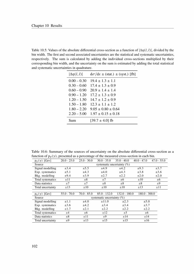
Chapter 10 Results
Table 10.5: Values of the absolute differential cross-section as a function of |Δ�휂(�푙, �푙) |, divided by thebin width. The first and second associated uncertainties are the statistical and systematic uncertainties,respectively. The sum is calculated by adding the individual cross-sections multiplied by theircorresponding bin width, and the uncertainty on the sum is estimated by adding the total statisticaland systematic uncertainties in quadrature.
|Δ�휂(�푙, �푙) | d�휎/d�푥 ± (stat.) ± (syst.) [fb]
0.00 – 0.30 19.4 ± 1.3 ± 1.10.30 – 0.60 17.4 ± 1.3 ± 0.90.60 – 0.90 20.9 ± 1.4 ± 1.40.90 – 1.20 17.2 ± 1.3 ± 0.91.20 – 1.50 14.7 ± 1.2 ± 0.91.50 – 1.80 12.3 ± 1.1 ± 1.21.80 – 2.20 9.05 ± 0.80 ± 0.642.20 – 5.00 1.97 ± 0.15 ± 0.18
Sum [39.7 ± 4.0] fb
Table 10.6: Summary of the sources of uncertainty on the absolute differential cross-section as afunction of pT(�훾), presented as a percentage of the measured cross-section in each bin.
pT (�훾) [Gev] 20.0 - 25.0 25.0 - 30.0 30.0 - 35.0 35.0 - 40.0 40.0 - 47.0 47.0 - 55.0Source systematic uncertainty (%)Signal modelling ±3.4 ±5.5 ±4.9 ±4.2 ±9.3 ±3.7
Exp. systematics ±5.1 ±4.3 ±4.0 ±4.3 ±3.8 ±3.6
Bkg. modelling ±9.4 ±3.9 ±2.7 ±2.2 ±2.0 ±2.0
Total systematics ±11 ±8 ±7 ±6 ±10 ±6
Data statistics ±7 ±7 ±8 ±8 ±8 ±9
Total uncertainty ±13 ±10 ±10 ±10 ±13 ±11
pT (�훾) [Gev] 55.0 - 70.0 70.0 - 85.0 85.0 - 132.0 132.0 - 180.0 180.0 - 300.0Source systematic uncertainty (%)Signal modelling ±1.1 ±4.0 ±11.0 ±2.3 ±5.0
Exp. systematics ±3.6 ±4.2 ±3.4 ±3.4 ±3.7
Bkg. modelling ±1.7 ±2.1 ±2.2 ±2.2 ±2.2
Total systematics ±4 ±6 ±12 ±5 ±6
Data statistics ±8 ±11 ±9 ±14 ±14
Total uncertainty ±9 ±13 ±15 ±15 ±16
102

10.1 Absolute cross-section measurements
Table 10.7: Summary of the sources of uncertainty on the absolute differential cross-section as afunction of |�휂(�훾) |, presented as a percentage of the measured cross-section in each bin.
|�휂 (�훾) | 0.0 - 0.2 0.2 - 0.4 0.4 - 0.6 0.6 - 0.8 0.8 - 1.0 1.0 - 1.2 1.2 - 1.7Source systematic uncertainty (%)Signal modelling ±1.6 ±2.8 ±6.2 ±6.3 ±2.5 ±5.6 ±2.8
Exp. systematics ±3.5 ±3.6 ±3.7 ±3.8 ±3.9 ±4.0 ±4.4
Bkg. modelling ±1.1 ±1.2 ±1.5 ±2.0 ±3.5 ±4.1 ±4.9
Total systematics ±4 ±5 ±7 ±7 ±5 ±8 ±7
Data statistics ±7 ±7 ±7 ±7 ±8 ±9 ±7
Total uncertainty ±8 ±8 ±10 ±10 ±10 ±12 ±10
|�휂 (�훾) | 1.7 - 2.37Source systematic uncertainty (%)Signal modelling ±3.9
Exp. systematics ±4.6
Bkg. modelling ±6.5
Total systematics ±9
Data statistics ±8
Total uncertainty ±12
Table 10.8: Summary of the sources of uncertainty on the absolute differential cross-section as afunction of Δ�푅(�훾, �푙)min, presented as a percentage of the measured cross-section in each bin.
Δ�푅 (�훾, �푙)min 0.4 - 0.55 0.55 - 0.7 0.7 - 0.85 0.85 - 1.0 1.0 - 1.3 1.3 - 1.6 1.6 - 1.9Source systematic uncertainty (%)Signal modelling ±5.3 ±3.5 ±1.5 ±8.2 ±4.1 ±2.9 ±3.5
Exp. systematics ±3.6 ±3.8 ±3.6 ±3.5 ±3.7 ±4.1 ±3.9
Bkg. modelling ±0.88 ±1.3 ±1.4 ±1.9 ±3.2 ±4.0 ±4.2
Total systematics ±6 ±5 ±4 ±9 ±6 ±6 ±7
Data statistics ±7 ±8 ±9 ±10 ±7 ±8 ±8
Total uncertainty ±10 ±9 ±10 ±14 ±9 ±10 ±10
Δ�푅 (�훾, �푙)min 1.9 - 2.3 2.3 - 2.7 2.7 - 5.0Source systematic uncertainty (%)Signal modelling ±3.9 ±2.1 ±7.7
Exp. systematics ±4.3 ±4.2 ±5.5
Bkg. modelling ±5.7 ±8.2 ±16.0
Total systematics ±8 ±9 ±19
Data statistics ±8 ±11 ±12
Total uncertainty ±11 ±14 ±23
103

Chapter 10 Results
Table 10.9: Summary of the sources of uncertainty on the absolute differential cross-sectionas a function of Δ�휙(�푙, �푙), presented as a percentage of the measured cross-section in each bin.
Δ�휙 (�푙, �푙) 0.0 - 0.6 0.6 - 1.2 1.2 - 1.6 1.6 - 1.9 1.9 - 2.2 2.2 - 2.4 2.4 - 2.6Source systematic uncertainty (%)Signal modelling ±6.9 ±1.1 ±4.2 ±5.1 ±2.4 ±3.3 ±7.0
Exp. systematics ±4.4 ±4.2 ±4.0 ±3.6 ±3.5 ±4.1 ±3.7
Bkg. modelling ±6.2 ±4.3 ±3.9 ±3.1 ±2.4 ±2.6 ±2.3
Total systematics ±10 ±6 ±7 ±7 ±5 ±6 ±8
Data statistics ±9 ±7 ±9 ±8 ±8 ±9 ±9
Total uncertainty ±13 ±9 ±11 ±11 ±9 ±11 ±12
Δ�휙 (�푙, �푙) 2.6 - 2.8 2.8 - 3.0 3.0 - 3.14Source systematic uncertainty (%)Signal modelling ±5.9 ±3.5 ±5.8
Exp. systematics ±4.0 ±3.7 ±4.5
Bkg. modelling ±2.5 ±2.4 ±2.1
Total systematics ±7 ±6 ±7
Data statistics ±9 ±9 ±10
Total uncertainty ±12 ±10 ±12
Table 10.10: Summary of the sources of uncertainty on the absolute differential cross-sectionas a function of |Δ�휂(�푙, �푙) |, presented as a percentage of the measured cross-section in each bin.
|Δ�휂 (�푙, �푙) | 0.0 - 0.3 0.3 - 0.6 0.6 - 0.9 0.9 - 1.2 1.2 - 1.5 1.5 - 1.8 1.8 - 2.2Source systematic uncertainty (%)Signal modelling ±1.9 ±2.0 ±4.1 ±2.4 ±4.2 ±8.4 ±5.3
Exp. systematics ±4.0 ±3.7 ±3.8 ±3.9 ±3.8 ±3.9 ±4.0
Bkg. modelling ±3.4 ±3.3 ±3.3 ±2.8 ±2.7 ±2.9 ±2.6
Total systematics ±6 ±5 ±7 ±5 ±6 ±10 ±7
Data statistics ±7 ±7 ±7 ±7 ±8 ±9 ±9
Total uncertainty ±9 ±9 ±9 ±9 ±10 ±13 ±11
|Δ�휂 (�푙, �푙) | 2.2 - 5.0Source systematic uncertainty (%)Signal modelling ±8.1
Exp. systematics ±4.4
Bkg. modelling ±2.4
Total systematics ±9
Data statistics ±7
Total uncertainty ±12
104

10.1 Absolute cross-section measurements
Figure 10.4: Statistical correlation matrix of the absolute fiducial cross-sections, estimated with thebootstrap method. Each bin is represented as < name >_bin< number >, where the name tag denotesthe observable’s name with ph_pt, ph_eta, dR_lep_ph, dEta_lep, and dPhi_lep referring to pT(�훾),|�휂(�훾) |, Δ�푅(�훾, �푙)min, |Δ�휂(�푙, �푙) | and Δ�휙(�푙, �푙), respectively. The number tag indicates the bin’s numberof the respective observable.
105
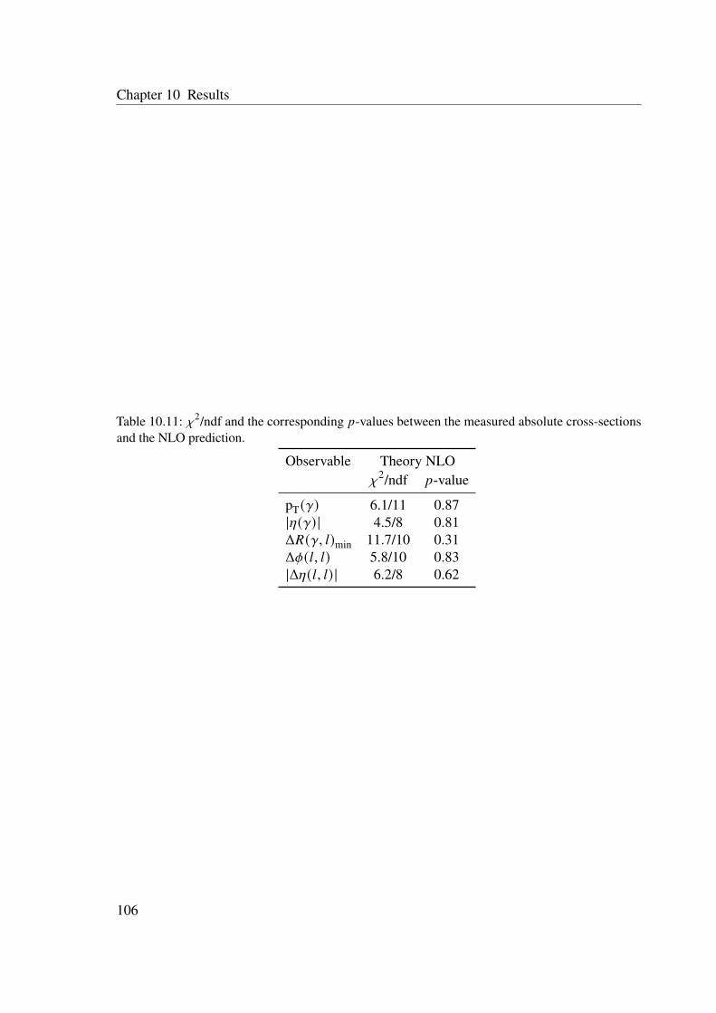
Chapter 10 Results
Table 10.11: �휒2/ndf and the corresponding �푝-values between the measured absolute cross-sectionsand the NLO prediction.
Observable Theory NLO
�휒2/ndf �푝-value
pT(�훾) 6.1/11 0.87|�휂(�훾) | 4.5/8 0.81Δ�푅(�훾, �푙)min 11.7/10 0.31Δ�휙(�푙, �푙) 5.8/10 0.83|Δ�휂(�푙, �푙) | 6.2/8 0.62
106
10.2 Normalised cross-section measurements
10.2 Normalised cross-section measurements
The unfolded distributions are normalised to their total integrals to benefit from the can-cellation of the normalisation components in the corresponding systematics while keepingthe components that change only the shapes of the distributions. The normalised fiducialdifferential cross-sections and the contribution of each category of systematic uncertainties asfunctions of pT(�훾), |�휂(�훾) |, Δ�푅(�훾, �푙)min, Δ�휙(�푙, �푙) and |Δ�휂(�푙, �푙) | are shown in Figs. 10.5–10.7.The top-row subfigures show the normalised cross-sections of unfolded data compared to thelatest NLO theory prediction [9] as well as state-of-the-art MC predictions of the combined�푡�푡�훾 + �푡�푊�훾 process, where the latter are generated at LO with MadGraph5_aMC@NLO andinterfaced with Pythia 8 and Herwig 7. The corresponding shaded bands represent thestatistical and the total uncertainties. The bottom-row subfigures display the decompositionof the systematic uncertainties and the statistical ones. The size of the uncertainties is reducedcompared to those of the absolute cross-sections in Figs. 10.1–10.3. As mentioned earlier,this is due to the cancellation of the normalisation components of the respective sources ofuncertainties while the shape components are kept. Similar to the absolute cross-sections, thenormalised distributions in the figures show the number of events divided by the bin width,and they do not include the overflow for pT(�훾), whereas for the rest of the distributions, thehigher boundary of the last bin is limited by the physical value. The shape of the measureddistributions as functions of pT(�훾), |�휂(�훾) |, and |Δ�휂(�푙, �푙) | shows a good agreement betweenthe unfolded data and the predictions within uncertainties. The NLO theory prediction welldescribes the shape of the measured distributions as functions of Δ�푅(�훾, �푙)min and Δ�휙(�푙, �푙),while the LO MC simulations do not model such shape perfectly. Both simulations ofMadGraph5_aMC@NLO interfaced with Pythia 8 and Herwig 7, exhibit similar behaviourin modelling the data, which weakens the possibility that the mis-modelling is caused due tothe showering algorithm.
The values of the normalised cross-sections and their associated uncertainties are listedin Tables 10.12–10.16. Similar to the absolute cross-sections, the statistical uncertainty isthe principal source, while the signal and background modelling dominate the systematicuncertainty.
The size of the systematic and statistical uncertainties are displayed in Tables 10.17–10.21.The total uncertainty is roughly in the range of 8%-10% for most of the normalised cross-sections of all variables (compared to 8%-12% for the absolute cross-sections). At highvalues of pT(�훾) and Δ�푅(�훾, �푙)min, it goes higher up to 15% and 21%, respectively (comparedto 16% and 23% for the pT(�훾) and Δ�푅(�훾, �푙)min absolute cross-sections, respectively).
The statistical correlation matrix of the normalised cross-sections of all observables,which is estimated using the bootstrap method, is shown in Fig. 10.8, where no significantcorrelation between different bins is observed. The full correlation matrices of the normalisedcross-sections as functions of all observables are shown in Appendix B.
The agreement between the unfolded data and the predictions for the normalised cross-sections is quantified using Eq. (10.1) with one ndf less by removing the last bin in the �휒
2
calculation.
107

Chapter 10 Results
The �휒2/ndf and the corresponding �푝-values for the normalised cross-sections are shown
in Table 10.22. The �푝-values between the data and the NLO prediction confirm the goodagreement between them for all the observables. Similarly, the �푝-values for the pT(�훾), |�휂(�훾) |,and |Δ�휂(�푙, �푙) | show a good agreement between the data and the MC predictions. However,for the Δ�푅(�훾, �푙)min and Δ�휙(�푙, �푙), the �푝-values between the data and the MC predictions arevery low (close to zero). These values verify that the modelling by the MC predictions is notperfectly compatible with the unfolded data for these observables.
[1 / G
eV
])
γ(T
d p
σd
⋅ σ1
-410
-310
-210
-110
1 Unfolded data
(MG5_aMC+Pythia8)γ+tWγtt
(MG5_aMC+Herwig7)γ+tWγtt
Theory NLO
Stat.
Syst.⊕Stat
-1 = 13 TeV, 139 fbs
Normalised cross-section
µe
) [GeV]γ(T
p
Pre
d./D
ata
0.81
1.2
) [GeV]γ(T
p50 100 150 200 250 300T
heory
/MC
0.95
1
1.05
)|γ(
ηd |
σd
⋅ σ1
0
0.2
0.4
0.6
0.8
1
1.2
1.4Unfolded data
(MG5_aMC+Pythia8)γ+tWγtt
(MG5_aMC+Herwig7)γ+tWγtt
Theory NLO
Stat.
Syst.⊕Stat
-1 = 13 TeV, 139 fbs
Normalised cross-section
µe
)|γ(η|
Pre
d./D
ata
0.81
1.2
)|γ(η|0 0.2 0.4 0.6 0.8 1 1.2 1.4 1.6 1.8 2 2.2T
heory
/MC
0.81
1.2
) [GeV]γ(T
p50 100 150 200 250 300
Fra
ctio
na
l u
nce
rta
inty
siz
e
-0.4
-0.2
0
0.2
0.4
0.6
Signal modelling Exp. systematics
Bkg. modelling
Stat. Syst.⊕Stat.
-1 = 13 TeV, 139 fbs
Normalised cross-section
µe
)|γ(η|0 0.2 0.4 0.6 0.8 1 1.2 1.4 1.6 1.8 2 2.2
Fra
ctio
na
l u
nce
rta
inty
siz
e
-0.3
-0.2
-0.1
0
0.1
0.2
0.3
0.4
Signal modelling Exp. systematics
Bkg. modelling
Stat. Syst.⊕Stat.
-1 = 13 TeV, 139 fbs
Normalised cross-section
µe
Figure 10.5: Distributions of the normalised fiducial differential cross-sections as functions of pT(�훾)and |�휂(�훾) | in the top row where unfolded data are compared to the NLO theory prediction [9], aswell MC predictions at LO which are generated with MadGraph5_aMC@NLO and interfaced withPythia 8 and Herwig 7. In the bottom row the statistical and systematic uncertainties are shown asfractions of the cross-section in each bin where the systematic uncertainties are decomposed into threecategories: signal, background, and experimental.
108

10.2 Normalised cross-section measurementsm
in)l,
γR
(∆
d
σd
⋅ σ1
0
0.2
0.4
0.6
0.8
1
1.2
1.4
1.6
1.8Unfolded data
(MG5_aMC+Pythia8)γ+tWγtt
(MG5_aMC+Herwig7)γ+tWγtt
Theory NLO
Stat.
Syst.⊕Stat
-1 = 13 TeV, 139 fbs
Normalised cross-section
µe
min)l,γR(∆
Pre
d./D
ata
0.5
1
1.5
min)l,γR(∆
0.5 1 1.5 2 2.5 3 3.5 4 4.5 5Theory
/MC
0.651
1.351.7
)l,l(φ
∆d
σd
⋅ σ1
0
0.2
0.4
0.6
0.8
1
1.2Unfolded data
(MG5_aMC+Pythia8)γ+tWγtt
(MG5_aMC+Herwig7)γ+tWγtt
Theory NLO
Stat.
Syst.⊕Stat
-1 = 13 TeV, 139 fbs
Normalised cross-section
µe
)l,l(φ∆
Pre
d./D
ata
0.5
1
1.5
)l,l(φ∆
0 0.5 1 1.5 2 2.5 3Theory
/MC
0.81
1.2
min)l,γR(∆
0.5 1 1.5 2 2.5 3 3.5 4 4.5 5
Fra
ctio
na
l u
nce
rta
inty
siz
e
-0.6
-0.4
-0.2
0
0.2
0.4
0.6
0.8
Signal modelling Exp. systematics
Bkg. modelling
Stat. Syst.⊕Stat.
-1 = 13 TeV, 139 fbs
Normalised cross-section
µe
)l,l(φ∆0 0.5 1 1.5 2 2.5 3
Fra
ctio
na
l u
nce
rta
inty
siz
e
-0.4
-0.3
-0.2
-0.1
0
0.1
0.2
0.3
0.4
0.5
Signal modelling Exp. systematics
Bkg. modelling
Stat. Syst.⊕Stat.
-1 = 13 TeV, 139 fbs
Normalised cross-section
µe
Figure 10.6: Distributions of the normalised fiducial differential cross-sections as functions ofΔ�푅(�훾, �푙)min and Δ�휙(�푙, �푙) in the top row where unfolded data are compared to the NLO theoryprediction [9], as well MC predictions at LO which are generated with MadGraph5_aMC@NLOand interfaced with Pythia 8 and Herwig 7. In the bottom row the statistical and systematicuncertainties are shown as fractions of the cross-section in each bin where the systematic uncertaintiesare decomposed into three categories: signal, background, and experimental.
109

Chapter 10 Results
)|l,l(η
∆d |
σd
⋅ σ1
0
0.2
0.4
0.6
0.8
1
1.2
1.4Unfolded data
(MG5_aMC+Pythia8)γ+tWγtt
(MG5_aMC+Herwig7)γ+tWγtt
Theory NLO
Stat.
Syst.⊕Stat
-1 = 13 TeV, 139 fbs
Normalised cross-section
µe
)|l,l(η∆|
Pre
d./D
ata
0.81
1.2
)|l,l(η∆|0 0.5 1 1.5 2 2.5 3 3.5 4 4.5 5T
heory
/MC
0.91
1.11.2
)|l,l(η∆|0 0.5 1 1.5 2 2.5 3 3.5 4 4.5 5
Fra
ctio
na
l u
nce
rta
inty
siz
e
-0.4
-0.3
-0.2
-0.1
0
0.1
0.2
0.3
0.4
0.5
Signal modelling Exp. systematics
Bkg. modelling
Stat. Syst.⊕Stat.
-1 = 13 TeV, 139 fbs
Normalised cross-section
µe
Figure 10.7: Distribution of the normalised fiducial differential cross-section as a function of |Δ�휂(�푙, �푙) |in the top row where unfolded data are compared to the NLO theory prediction [9], as well MCpredictions at LO which are generated with MadGraph5_aMC@NLO and interfaced with Pythia 8and Herwig 7. In the bottom row the statistical and systematic uncertainties are shown as fractions ofthe cross-section in each bin where the systematic uncertainties are decomposed into three categories:signal, background, and experimental.
110

10.2 Normalised cross-section measurements
Table 10.12: Values of the normalised differential cross-section as a function of pT(�훾), divided by thebin width. The first and second associated uncertainties are the statistical and systematic uncertainties,respectively.
pT(�훾) [Gev] 1/�휎 · d�휎/d�푥 ± (stat.) ± (syst.) [1/GeV]
20 – 25 0.0447 ± 0.0029 ± 0.003925 – 30 0.0333 ± 0.0022 ± 0.000930 – 35 0.0243 ± 0.0018 ± 0.000635 – 40 0.0177 ± 0.0015 ± 0.000640 – 47 0.0119 ± 0.0010 ± 0.000847 – 55 0.00836 ± 0.00079 ± 0.0003855 – 70 0.00554 ± 0.00047 ± 0.0002570 – 85 0.00305 ± 0.00034 ± 0.0001285 – 132 0.00151 ± 0.00013 ± 0.00013132 – 180 0.000501 ± 0.000072 ± 0.000019180 – 300 0.000212 ± 0.000029 ± 0.000012
Table 10.13: Values of the normalised differential cross-section as a function of |�휂(�훾) |, divided by thebin width. The first and second associated uncertainties are the statistical and systematic uncertainties,respectively.
|�휂(�훾) | 1/�휎 · d�휎/d�푥 ± (stat.) ± (syst.)
0.00 – 0.20 0.637 ± 0.045 ± 0.0220.20 – 0.40 0.642 ± 0.045 ± 0.0220.40 – 0.60 0.575 ± 0.042 ± 0.0200.60 – 0.80 0.600 ± 0.044 ± 0.0190.80 – 1.00 0.489 ± 0.040 ± 0.0081.00 – 1.20 0.418 ± 0.036 ± 0.0101.20 – 1.70 0.389 ± 0.028 ± 0.0131.70 – 2.37 0.199 ± 0.015 ± 0.008
111

Chapter 10 Results
Table 10.14: Values of the normalised differential cross-section as a function of Δ�푅(�훾, �푙)min, dividedby the bin width. The first and second associated uncertainties are the statistical and systematicuncertainties, respectively.
Δ�푅(�훾, �푙)min 1/�휎 · d�휎/d�푥 ± (stat.) ± (syst.)
0.40 – 0.55 0.921 ± 0.066 ± 0.0320.55 – 0.70 0.720 ± 0.057 ± 0.0190.70 – 0.85 0.596 ± 0.053 ± 0.0190.85 – 1.00 0.484 ± 0.048 ± 0.0241.00 – 1.30 0.455 ± 0.032 ± 0.0141.30 – 1.60 0.367 ± 0.029 ± 0.0101.60 – 1.90 0.390 ± 0.030 ± 0.0091.90 – 2.30 0.267 ± 0.022 ± 0.0092.30 – 2.70 0.162 ± 0.018 ± 0.0102.70 – 5.00 0.0248 ± 0.0029 ± 0.0043
Table 10.15: Values of the normalised differential cross-section as a function of Δ�휙(�푙, �푙), dividedby the bin width. The first and second associated uncertainties are the statistical and systematicuncertainties, respectively.
Δ�휙(�푙, �푙) 1/�휎 · d�휎/d�푥 ± (stat.) ± (syst.)
0.00 – 0.60 0.190 ± 0.016 ± 0.0110.60 – 1.20 0.247 ± 0.018 ± 0.0091.20 – 1.60 0.262 ± 0.022 ± 0.0051.60 – 1.90 0.342 ± 0.029 ± 0.0071.90 – 2.20 0.376 ± 0.029 ± 0.0202.20 – 2.40 0.399 ± 0.038 ± 0.0082.40 – 2.60 0.449 ± 0.039 ± 0.0182.60 – 2.80 0.428 ± 0.038 ± 0.0142.80 – 3.00 0.455 ± 0.039 ± 0.0103.00 – 3.14 0.508 ± 0.049 ± 0.018
112

10.2 Normalised cross-section measurements
Table 10.16: Values of the normalised differential cross-section as a function of |Δ�휂(�푙, �푙) |, dividedby the bin width. The first and second associated uncertainties are the statistical and systematicuncertainties, respectively.
|Δ�휂(�푙, �푙) | 1/�휎 · d�휎/d�푥 ± (stat.) ± (syst.)
0.00 – 0.30 0.488 ± 0.034 ± 0.0140.30 – 0.60 0.439 ± 0.032 ± 0.0100.60 – 0.90 0.527 ± 0.035 ± 0.0200.90 – 1.20 0.432 ± 0.032 ± 0.0071.20 – 1.50 0.370 ± 0.029 ± 0.0061.50 – 1.80 0.311 ± 0.027 ± 0.0151.80 – 2.20 0.228 ± 0.020 ± 0.0082.20 – 5.00 0.0496 ± 0.0037 ± 0.0026
Table 10.17: Summary of the sources of uncertainty on the normalised differential cross-section as afunction of pT(�훾), presented as a percentage of the measured cross-section in each bin.
pT (�훾) [Gev] 20.0 - 25.0 25.0 - 30.0 30.0 - 35.0 35.0 - 40.0 40.0 - 47.0 47.0 - 55.0Source systematic uncertainty (%)Signal modelling ±5.5 ±2.5 ±2.1 ±1.5 ±6.2 ±3.6
Exp. systematics ±1.6 ±1.0 ±0.98 ±1.9 ±0.9 ±1.3
Bkg. modelling ±6.7 ±0.9 ±1.0 ±2.2 ±2.6 ±2.5
Total systematics ±9 ±3 ±3 ±3 ±7 ±5
Data statistics ±7 ±7 ±8 ±8 ±8 ±9
Total uncertainty ±11 ±7 ±8 ±9 ±11 ±10
pT (�훾) [Gev] 55.0 - 70.0 70.0 - 85.0 85.0 - 132.0 132.0 - 180.0 180.0 - 300.0Source systematic uncertainty (%)Signal modelling ±3.3 ±2.1 ±8.1 ±1.5 ±3.7
Exp. systematics ±1.1 ±2.0 ±1.7 ±2.0 ±3.1
Bkg. modelling ±2.8 ±2.8 ±3.1 ±3.0 ±3.1
Total systematics ±5 ±4 ±9 ±4 ±6
Data statistics ±8 ±11 ±9 ±14 ±14
Total uncertainty ±10 ±12 ±13 ±15 ±15
113

Chapter 10 Results
Table 10.18: Summary of the sources of uncertainty on the normalised differential cross-section as afunction of |�휂(�훾) |, presented as a percentage of the measured cross-section in each bin.
|�휂 (�훾) | 0.0 - 0.2 0.2 - 0.4 0.4 - 0.6 0.6 - 0.8 0.8 - 1.0 1.0 - 1.2 1.2 - 1.7Source systematic uncertainty (%)Signal modelling ±2.7 ±2.7 ±2.8 ±2.8 ±1.1 ±2.1 ±2.2
Exp. systematics ±0.86 ±0.91 ±0.85 ±0.95 ±0.98 ±0.68 ±1.3
Bkg. modelling ±1.9 ±2.0 ±1.7 ±1.2 ±0.75 ±1.2 ±2.1
Total systematics ±3 ±4 ±3 ±3 ±2 ±3 ±3
Data statistics ±7 ±7 ±7 ±7 ±8 ±9 ±7
Total uncertainty ±8 ±8 ±8 ±8 ±8 ±9 ±8
|�휂 (�훾) | 1.7 - 2.37Source systematic uncertainty (%)Signal modelling ±0.68
Exp. systematics ±1.3
Bkg. modelling ±3.8
Total systematics ±4
Data statistics ±8
Total uncertainty ±9
Table 10.19: Summary of the sources of uncertainty on the normalised differential cross-section as afunction of Δ�푅(�훾, �푙)min, presented as a percentage of the measured cross-section in each bin.
Δ�푅 (�훾, �푙)min 0.4 - 0.55 0.55 - 0.7 0.7 - 0.85 0.85 - 1.0 1.0 - 1.3 1.3 - 1.6 1.6 - 1.9Source systematic uncertainty (%)Signal modelling ±1.8 ±0.75 ±2.2 ±4.7 ±2.0 ±0.78 ±1.1
Exp. systematics ±0.61 ±0.59 ±0.8 ±0.93 ±0.56 ±0.87 ±0.73
Bkg. modelling ±2.8 ±2.4 ±2.0 ±1.5 ±2.3 ±2.5 ±1.9
Total systematics ±4 ±3 ±3 ±5 ±3 ±3 ±2
Data statistics ±7 ±8 ±9 ±10 ±7 ±8 ±8
Total uncertainty ±8 ±8 ±9 ±11 ±8 ±8 ±8
Δ�푅 (�훾, �푙)min 1.9 - 2.3 2.3 - 2.7 2.7 - 5.0Source systematic uncertainty (%)Signal modelling ±2.0 ±1.6 ±9.3
Exp. systematics ±0.75 ±1.1 ±2.7
Bkg. modelling ±3.0 ±5.8 ±15.0
Total systematics ±4 ±6 ±17
Data statistics ±8 ±11 ±12
Total uncertainty ±9 ±12 ±21
114

10.2 Normalised cross-section measurements
Table 10.20: Summary of the sources of uncertainty on the normalised differential cross-section as afunction of Δ�휙(�푙, �푙), presented as a percentage of the measured cross-section in each bin.
Δ�휙 (�푙, �푙) 0.0 - 0.6 0.6 - 1.2 1.2 - 1.6 1.6 - 1.9 1.9 - 2.2 2.2 - 2.4 2.4 - 2.6Source systematic uncertainty (%)Signal modelling ±3.9 ±3.1 ±1.5 ±1.7 ±5.2 ±1.4 ±3.6
Exp. systematics ±1.3 ±1.1 ±0.84 ±0.92 ±0.76 ±1.2 ±1.3
Bkg. modelling ±3.8 ±1.9 ±1.1 ±0.6 ±0.72 ±0.81 ±0.98
Total systematics ±6 ±4 ±2 ±2 ±5 ±2 ±4
Data statistics ±9 ±7 ±9 ±8 ±8 ±9 ±9
Total uncertainty ±10 ±8 ±9 ±9 ±9 ±10 ±10
Δ�휙 (�푙, �푙) 2.6 - 2.8 2.8 - 3.0 3.0 - 3.14Source systematic uncertainty (%)Signal modelling ±2.9 ±1.4 ±2.7
Exp. systematics ±0.82 ±0.92 ±1.6
Bkg. modelling ±0.98 ±1.4 ±1.7
Total systematics ±3 ±2 ±4
Data statistics ±9 ±9 ±10
Total uncertainty ±9 ±9 ±10
Table 10.21: Summary of the sources of uncertainty on the normalised differential cross-section as afunction of |Δ�휂(�푙, �푙) |, presented as a percentage of the measured cross-section in each bin.
|Δ�휂 (�푙, �푙) | 0.0 - 0.3 0.3 - 0.6 0.6 - 0.9 0.9 - 1.2 1.2 - 1.5 1.5 - 1.8 1.8 - 2.2Source systematic uncertainty (%)Signal modelling ±2.6 ±1.8 ±3.7 ±1.2 ±1.3 ±4.9 ±3.3
Exp. systematics ±0.75 ±0.98 ±0.87 ±0.87 ±0.52 ±0.63 ±0.88
Bkg. modelling ±1.1 ±0.79 ±0.53 ±0.29 ±0.58 ±0.77 ±0.76
Total systematics ±3 ±2 ±4 ±2 ±2 ±5 ±4
Data statistics ±7 ±7 ±7 ±7 ±8 ±9 ±9
Total uncertainty ±8 ±8 ±8 ±8 ±8 ±10 ±10
|Δ�휂 (�푙, �푙) | 2.2 - 5.0Source systematic uncertainty (%)Signal modelling ±4.9
Exp. systematics ±1.4
Bkg. modelling ±1.1
Total systematics ±5
Data statistics ±7
Total uncertainty ±9
115

Chapter 10 Results
Figure 10.8: Statistical correlation matrix of the normalised fiducial cross-sections, estimated with thebootstrap method. Each bin is represented as < name >_bin< number >, where the name tag denotesthe observable’s name with ph_pt, ph_eta, dR_lep_ph, dEta_lep, and dPhi_lep referring to pT(�훾),|�휂(�훾) |, Δ�푅(�훾, �푙)min, |Δ�휂(�푙, �푙) | and Δ�휙(�푙, �푙), respectively. The number tag indicates the bin’s numberof the respective observable.
116
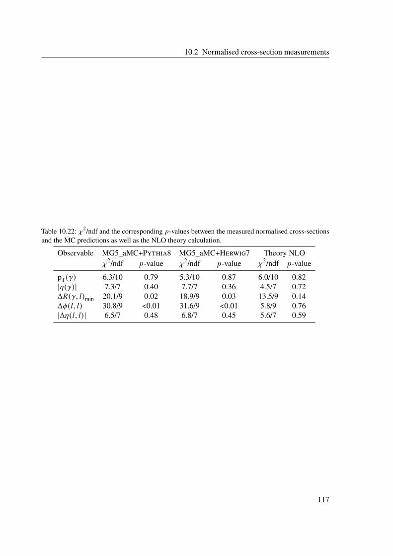
10.2 Normalised cross-section measurements
Table 10.22: �휒2/ndf and the corresponding �푝-values between the measured normalised cross-sectionsand the MC predictions as well as the NLO theory calculation.
Observable MG5_aMC+Pythia8 MG5_aMC+Herwig7 Theory NLO
�휒2/ndf �푝-value �휒
2/ndf �푝-value �휒2/ndf �푝-value
pT(�훾) 6.3/10 0.79 5.3/10 0.87 6.0/10 0.82|�휂(�훾) | 7.3/7 0.40 7.7/7 0.36 4.5/7 0.72Δ�푅(�훾, �푙)min 20.1/9 0.02 18.9/9 0.03 13.5/9 0.14Δ�휙(�푙, �푙) 30.8/9 <0.01 31.6/9 <0.01 5.8/9 0.76|Δ�휂(�푙, �푙) | 6.5/7 0.48 6.8/7 0.45 5.6/7 0.59
117


CHAPTER 11
Conclusions and outlook
This work presents differential cross-section measurements of the combined �푡�푡�훾 + �푡�푊�훾
process in the �푒�휇 decay channel. The measurements are performed in this decay channel dueto its high signal purity and to compare with the most recent theory calculation at NLO inQCD [9]. The data used in this work were collected by the ATLAS detector at the LHC in�푝�푝 collisions at
√�푠 = 13 TeV, with an integrated luminosity of 139 fb
−1.
The signal region of the measurements is characterised by the presence of exactly one hardphoton, one electron and one muon of opposite charge, at least two jets among which at leastone is �푏-tagged, and missing transverse energy. The reconstructed distributions of data arecorrected for acceptance and efficiencies of the detector using the IBS unfolding method.The performance of the IBS method is tested and optimised, leading to a reliable unfoldingprocedure.
The differential measurements are performed in a fiducial phase space at parton level,as functions of pT(�훾), |�휂(�훾) |, Δ�푅(�훾, �푙)min, Δ�휙(�푙, �푙), and |Δ�휂(�푙, �푙) |. Fiducial phase-spacerequirements mimic the selection in the dedicated theoretical calculation, provided by theauthors of Ref. [9].
For the first time, the combined �푡�푡�훾 + �푡�푊�훾 cross-section measurements are comparedto a full calculation at NLO in QCD, including resonant and non-resonant contributionsand off-shell effects. Furthermore, the measurements are compared to state-of-the-art MCsimulations at LO in QCD. They are found to be in good agreement with the calculation andthe MC simulations within uncertainties. The overall shape of the measured distributions isdescribed better by the calculation than the MC simulations, especially for the Δ�푅(�훾, �푙)minand Δ�휙(�푙, �푙) distributions.
The precision of the results presented here surpasses that of the differential measurementsperformed at an integrated luminosity of 36 fb
−1 [7]. However, results can not be directlycompared since they are performed in a different fiducial phase space. The results haveoverall total uncertainties of approximately 8%-12% and 8%-10% for most absolute andnormalised differential cross-sections, respectively. Only in regions with a small numberof events, such as at high values of pT(�훾) and Δ�푅(�훾, �푙)min, the total uncertainty increases
119

Chapter 11 Conclusions and outlook
to 16% and 23%, respectively, for the absolute cross-sections and 15% and 21%, for thenormalised ones. Statistical uncertainties limit the precision of the measurements, whereassignal and background modelling dominate the systematic uncertainties.
The measurements presented here are compared with the NLO theory calculation focusingon the �푒�휇 channel. The statistical uncertainty for future measurements, being the limiting factor,can be reduced by including more decay channels, with minor background contaminations,such as the �푒�푒 and �휇�휇 channels, i.e. performing the measurements in the full dileptonchannel. Despite having relatively small BRs, these decay channels combined, i.e. �푒�푒 and�휇�휇, would still double the number of collected data events. Furthermore, having a smallbackground contribution would mean that the uncertainties related to background processeswill not outperform the possible decrease in the statistical uncertainty. Moreover, systematicuncertainties of the measurements presented in this work approach in size the statisticalones. Hence, using an unfolding procedure that correlates the sources of uncertainties, e.g.employing a fit where the uncertainties are included as nuisance parameters, can lessen suchsystematic uncertainties. For example, techniques such as a likelihood profiling based onHistFitter [116] and Fully Bayesian Unfolding [117] offer such advantage.
The modelling of Δ�푅(�훾, �푙)min and Δ�휙(�푙, �푙) distributions by the MC simulations at LO inQCD requires further investigation, and higher-order corrections are needed to describe thedata better. Additionally, other measurements can be performed using the full Run 2 data inthe single lepton and dilepton channels. Such measurements with a large number of dataevents can unravel the possibility to perform double-differential measurements, for example,as a function of pT(�훾) in different |�휂(�훾) | regions. These measurements are sensitive to thegluon parton distribution functions.
The differential measurements can be interpreted in effective field theories by testinghigher-dimensional operators sensitive to the �푡�푡�훾 vertex [39]. Such an interpretation wouldbe a stringent test to SM predictions where any deviation would point to new physics.
120

Bibliography
[1] CDF Collaboration, Observation of Top Quark Production in pp Collisions with the
Collider Detector at Fermilab, Phys. Rev. Lett. 74 (14 1995) 2626 (cit. on p. 1).
[2] D0 Collaboration, Observation of the Top Quark, Phys. Rev. Lett. 74 (14 1995) 2632(cit. on p. 1).
[3] CDF Collaboration, Evidence for �푡�푡�훾 production and measurement of �휎�푡�푡�훾/�휎�푡�푡 ,Phys. Rev. D 84 (2011) (cit. on p. 1).
[4] ATLAS Collaboration, Observation of top-quark pair production in association with
a photon and measurement of the �푡�푡�훾 production cross section in �푝�푝 collisions at√�푠 = 7 TeV using the ATLAS detector, Phys. Rev. D 91 (7 2015) 072007 (cit. on p. 1).
[5] ATLAS Collaboration, Measurement of the �푡�푡�훾 production cross section in
proton-proton collisions at√�푠 = 8 TeV with the ATLAS detector,
JHEP 11 (2017) 086, arXiv: 1706.03046 [hep-ex] (cit. on p. 1).
[6] CMS Collaboration, Measurement of the semileptonic �푡�푡 + �훾 production cross section
in �푝�푝 collisions at√�푠 = 8 TeV, JHEP 10 (2017) 006, arXiv: 1706.08128 [hep-ex]
(cit. on p. 1).
[7] ATLAS Collaboration, Measurements of inclusive and differential fiducial
cross-sections of �푡�푡�훾 production in leptonic final states at√�푠 = 13 TeV in ATLAS,
Eur. Phys. J. C 79 (2019), arXiv: 1812.01697 [hep-ex] (cit. on pp. 1, 58, 119).
[8] ATLAS Collaboration,Measurements of inclusive and differential cross-sections of combined �푡�푡�훾 and �푡�푊�훾
production in the e�휇 channel at 13 TeV with the ATLAS detector,JHEP 09 (2020) 049, arXiv: 2007.06946 [hep-ex] (cit. on pp. 2, 95).
[9] G. Bevilacqua et al.,Hard photons in hadroproduction of top quarks with realistic final states,JHEP 10 (2018) 158, arXiv: 1803.09916 [hep-ph](cit. on pp. 2, 12–14, 51, 57, 61, 62, 95, 97–99, 107–110, 119).
[10] H. D. Politzer, Reliable Perturbative Results for Strong Interactions?,Phys. Rev. Lett. 30 (26 1973) 1346 (cit. on p. 3).
[11] D. J. Gross and F. Wilczek, Asymptotically Free Gauge Theories. I,Phys. Rev. D 8 (10 1973) 3633 (cit. on p. 3).
121

Bibliography
[12] H. David Politzer, Asymptotic freedom: An approach to strong interactions,Phys. Rep. 14 (1974) 129 (cit. on p. 3).
[13] S. L. Glashow, Partial-symmetries of weak interactions, Nucl. Phys. 22 (1961) 579(cit. on pp. 3, 6).
[14] A. Salam and J. C. Ward, Electromagnetic and weak interactions,Phys. Lett. 13 (1964) 168 (cit. on pp. 3, 6).
[15] S. Weinberg, A Model of Leptons, Phys. Rev. Lett. 19 (21 1967) 1264(cit. on pp. 3, 6).
[16] Wikimedia Commons, Standard Model of Elementary Particles and Gravity, 2017,url: https://commons.wikimedia.org/w/index.php?curid=59970304(cit. on p. 4).
[17] M. Tanabashi et al., Review of Particle Physics, Phys. Rev. D 98 (2018)(cit. on pp. 6, 8).
[18] D. J. Gross and F. Wilczek, Ultraviolet Behavior of Non-Abelian Gauge Theories,Phys. Rev. Lett. 30 (1973) 1343 (cit. on p. 5).
[19] ALEPH Collaboration, CDF Collaboration, D0 Collaboration, DELPHICollaboration, L3 Collaboration, OPAL Collaboration, SLD Collaboration, LEPElectroweak Working Group, Tevatron Electroweak Working Group, SLDelectroweak and heavy flavour groups,Precision Electroweak Measurements and Constraints on the Standard Model, 2011,arXiv: 1012.2367 [hep-ex] (cit. on p. 7).
[20] P. W. Higgs, Broken Symmetries and the Masses of Gauge Bosons,Phys. Rev. Lett. 13 (16 1964) 508 (cit. on p. 7).
[21] P. W. Higgs, Broken symmetries, massless particles and gauge fields,Phys. Lett. 12 (1964) 132 (cit. on p. 7).
[22] F. Englert and R. Brout, Broken Symmetry and the Mass of Gauge Vector Mesons,Phys. Rev. Lett. 13 (9 1964) 321 (cit. on p. 7).
[23] G. S. Guralnik, C. R. Hagen and T. W. B. Kibble,Global Conservation Laws and Massless Particles, Phys. Rev. Lett. 13 (20 1964) 585(cit. on p. 7).
[24] ATLAS Collaboration, Observation of a new particle in the search for the Standard
Model Higgs boson with the ATLAS detector at the LHC, Phys. Lett. B 716 (2012) 1(cit. on pp. 7, 17).
[25] CMS Collaboration, Observation of a new boson at a mass of 125 GeV with the CMS
experiment at the LHC, Phys. Lett. B 716 (2012) 30 (cit. on pp. 7, 17).
[26] ATLAS, CDF, CMS and D0 Collaborations,First combination of Tevatron and LHC measurements of the top-quark mass, 2014,arXiv: 1403.4427 [hep-ex] (cit. on p. 7).
122

[27] J. C. Collins, D. E. Soper and G. F. Sterman,Factorization of Hard Processes in QCD,Adv. Ser. Direct. High Energy Phys. 5 (1989) 1, arXiv: hep-ph/0409313(cit. on p. 7).
[28] J. D. Bjorken, Asymptotic Sum Rules at Infinite Momentum,Phys. Rev. 179 (5 1969) 1547 (cit. on p. 7).
[29] J. D. Bjorken and E. A. Paschos,Inelastic Electron-Proton and �훾-Proton Scattering and the Structure of the Nucleon,Phys. Rev. 185 (5 1969) 1975 (cit. on p. 7).
[30] R. P. Feynman, Very High-Energy Collisions of Hadrons,Phys. Rev. Lett. 23 (24 1969) 1415 (cit. on p. 7).
[31] M. Czakon and A. Mitov, Top++: A program for the calculation of the top-pair
cross-section at hadron colliders, Comput. Phys. Commun. 185 (2014) 2930,arXiv: 1112.5675 [hep-ph] (cit. on pp. 8, 53).
[32] LHCTopWG,NLO single-top channel cross sections: ATLAS-CMS recommended predictions for
single-top cross sections using the Hathor v2.1 program (topic revision: r34), 2017,url: https://twiki.cern.ch/twiki/bin/view/LHCPhysics/SingleTopRefXsec
(cit. on p. 9).
[33] M. Aliev et al.,HATHOR – HAdronic Top and Heavy quarks crOss section calculatoR,Comput. Phys. Commun. 182 (2011) 1034, arXiv: 1007.1327 [hep-ph](cit. on p. 9).
[34] P. Kant et al., HATHOR for single top-quark production: Updated predictions and
uncertainty estimates for single top-quark production in hadronic collisions,Comput. Phys. Commun. 191 (2015) 74, arXiv: 1406.4403 [hep-ph] (cit. on p. 9).
[35] K. Olive, Review of Particle Physics, Chin. Phys. C 40 (2016) 100001 (cit. on p. 9).
[36] D0 Collaboration, Useful Diagrams of Top Signals and Backgrounds, 2011,url: https://www-d0.fnal.gov/Run2Physics/top/top_public_web_pages/top_feynman_diagrams.html (cit. on p. 10).
[37] S. M. Etesami, S. Khatibi and M. M. Najafabadi,Measuring anomalous �푊�푊�훾 and �푡�푡�훾 couplings using top+�훾 production at the LHC,Eur. Phys. J. C 76 (2016), arXiv: 1606.02178 [hep-ex] (cit. on p. 10).
[38] U. Baur et al.,Probing electroweak top quark couplings at hadron and lepton colliders,Nucl. Phys. B Proc. Suppl. 160 (2006) 17, arXiv: hep-ph/0606264 (cit. on p. 10).
123
Bibliography
[39] O. Bessidskaia Bylund et al., Probing top quark neutral couplings in the Standard
Model Effective Field Theory at NLO in QCD, JHEP 05 (2016) 052,arXiv: 1601.08193 [hep-ph] (cit. on pp. 10, 120).
[40] P.-F. Duan et al.,QCD corrections to associated production of �푡�푡�훾 at hadron colliders,Phys. Rev. D 80 (1 2009) 014022 (cit. on p. 11).
[41] K. Melnikov, M. Schulze and A. Scharf, QCD corrections to top quark pair
production in association with a photon at hadron colliders,Phys. Rev. D 83 (7 2011) 074013 (cit. on p. 11).
[42] V. S. Fadin, V. A. Khoze and A. D. Martin,Interference radiative phenomena in the production of heavy unstable particles,Phys. Rev. D 49 (5 1994) 2247 (cit. on p. 11).
[43] K. Melnikov and O. Yakovlev, Top near threshold: all α�푆 corrections are trivial,Phys. Lett. B 324 (1994) 217 (cit. on p. 11).
[44] K. Melnikov and O. Yakovlev,Final state interaction in the production of heavy unstable particles,Nucl. Phys. B 471 (1996) 90 (cit. on p. 11).
[45] S. Dulat et al., New parton distribution functions from a global analysis of quantum
chromodynamics, Phys. Rev. D 93 (2016) 033006, arXiv: 1506.07443 [hep-ph](cit. on p. 13).
[46] ATLAS Collaboration,ATLAS detector and physics performance: Technical Design Report, 1,CERN-LHCC-99-014, ATLAS-TDR-14, CERN, 1999,url: https://cds.cern.ch/record/391176 (cit. on p. 15).
[47] ATLAS detector and physics performance: Technical Design Report, 2,CERN-LHCC-99-015, ATLAS-TDR-15, CERN, 1999,url: https://cds.cern.ch/record/391177 (cit. on p. 15).
[48] CMS Collaboration, CMS Physics: Technical Design Report Volume 1: Detector
Performance and Software, CERN-LHCC-2006-001, CMS-TDR-8-1, CERN, 2006,url: https://cds.cern.ch/record/922757 (cit. on p. 15).
[49] LHCb Collaboration, LHCb : Technical Proposal,CERN-LHCC-98-004, LHCC-P-4, CERN, 1998,url: https://cds.cern.ch/record/622031 (cit. on p. 15).
[50] ALICE Collaboration,ALICE: Technical proposal for a Large Ion collider Experiment at the CERN LHC,CERN-LHCC-95-71, LHCC-P-3, CERN, 1995,url: http://cds.cern.ch/record/293391 (cit. on p. 15).
124

[51] C. Lefévre, The CERN Accelerator Complex. Complexe des accélérateurs du CERN,url: http://cds.cern.ch/record/1260465 (cit. on p. 16).
[52] ATLAS Collaboration, Reconstruction of primary vertices at the ATLAS experiment
in Run 1 proton–proton collisions at the LHC, Eur. Phys. J. C77 (2017) 332,arXiv: 1611.10235 [physics.ins-det] (cit. on pp. 17, 31).
[53] ATLAS Collaboration, The ATLAS Experiment at the CERN Large Hadron Collider,JINST 3 (2008) S08003 (cit. on pp. 18, 20, 22).
[54] ATLAS Collaboration, Performance of the ATLAS track reconstruction algorithms in
dense environments in LHC Run 2, Eur. Phys. J. C 77 (2017) (cit. on p. 20).
[55] E. Diehl, Calibration and Performance of the ATLAS Muon Spectrometer, 2011,arXiv: 1109.6933 [physics.ins-det] (cit. on p. 23).
[56] ATLAS Collaboration, Performance of the ATLAS trigger system in 2015,Eur. Phys. J. C 77 (2017), arXiv: 1611.09661 [hep-ex] (cit. on p. 23).
[57] ATLAS Collaboration,Electron reconstruction and identification in the ATLAS experiment using the 2015
and 2016 LHC proton–proton collision data at√�푠 = 13 TeV,
Eur. Phys. J. C79 (2019) 639, arXiv: 1902.04655 [physics.ins-det](cit. on pp. 26, 27, 30, 39).
[58] W. Lampl et al., Calorimeter Clustering Algorithms: Description and Performance,ATL-LARG-PUB-2008-002, ATL-COM-LARG-2008-003, CERN, 2008,url: https://cds.cern.ch/record/1099735 (cit. on p. 26).
[59] T. Cornelissen et al., The global �휒2
track fitter in ATLAS,J. Phys. Conf. Ser. 119 (2008) 032013 (cit. on p. 26).
[60] ATLAS Collaboration, Electron and photon performance measurements with the
ATLAS detector using the 2015–2017 LHC proton–proton collision data,JINST 14 (2019) P12006, arXiv: 1908.00005 [hep-ex] (cit. on pp. 26, 89).
[61] ATLAS Collaboration, Muon reconstruction performance of the ATLAS detector in
proton–proton collision data at√�푠 = 13 TeV, Eur. Phys. J. C76 (2016) 292,
arXiv: 1603.05598 [hep-ex] (cit. on pp. 27, 29, 89).
[62] ATLAS Collaboration, Electron and photon energy calibration with the ATLAS
detector using 2015–2016 LHC proton–proton collision data,JINST 14 (2019) P03017, arXiv: 1812.03848 [hep-ex] (cit. on p. 30).
[63] M. Cacciari, G. P. Salam and G. Soyez, The anti-�푘�푡 jet clustering algorithm,JHEP 04 (2008) 063, arXiv: 0802.1189 [hep-ph] (cit. on pp. 31, 32).
[64] ATLAS Collaboration, Topological cell clustering in the ATLAS calorimeters and its
performance in LHC Run 1, Eur. Phys. J. C 77 (2017) 490,arXiv: 1603.02934 [hep-ex] (cit. on p. 31).
125

Bibliography
[65] S. D. Ellis and D. E. Soper,Successive combination jet algorithm for hadron collisions,Phys. Rev. D 48 (1993) 3160 (cit. on p. 32).
[66] M. Cacciari, G. P. Salam and G. Soyez, FastJet user manual,Eur. Phys. J. C 72 (2012) 1896, arXiv: 1111.6097 [hep-ph] (cit. on p. 32).
[67] ATLAS Collaboration, Jet energy scale measurements and their systematic
uncertainties in proton-proton collisions at√�푠 = 13 TeV with the ATLAS detector,
Phys. Rev. D 96 (2017) 072002 (cit. on p. 33).
[68] ATLAS Collaboration, Measurements of b-jet tagging efficiency with the ATLAS
detector using �푡�푡 events at√�푠 = 13 TeV, JHEP 08 (2018) 089,
arXiv: 1805.01845 [hep-ex] (cit. on pp. 34, 90).
[69] ATLAS Collaboration, Optimisation and performance studies of the ATLAS
�푏-tagging algorithms for the 2017-18 LHC run, ATL-PHYS-PUB-2017-013,CERN, 2017, url: https://cds.cern.ch/record/2273281 (cit. on p. 34).
[70] ATLAS Collaboration,Secondary vertex finding for jet flavour identification with the ATLAS detector,ATL-PHYS-PUB-2017-011, CERN, 2017,url: https://cds.cern.ch/record/2270366 (cit. on p. 34).
[71] ATLAS Collaboration, Topological �푏-hadron decay reconstruction and identification
of �푏-jets with the JetFitter package in the ATLAS experiment at the LHC,ATL-PHYS-PUB-2018-025, CERN, 2018,url: https://cds.cern.ch/record/2645405 (cit. on p. 34).
[72] ATLAS Collaboration, Performance of missing transverse momentum reconstruction
with the ATLAS detector using proton-proton collisions at√�푠 = 13 TeV,
Eur. Phys. J. C 78 (2018) 903, arXiv: 1802.08168 [hep-ex] (cit. on p. 34).
[73] A. D. Martin et al., Parton distributions for the LHC, Eur. Phys. J. C 63 (2009) 189,arXiv: 0901.0002 [hep-ph] (cit. on pp. 37, 53).
[74] H.-L. Lai et al., New parton distributions for collider physics,Phys. Rev. D 82 (7 2010) 074024,url: https://link.aps.org/doi/10.1103/PhysRevD.82.074024(cit. on p. 37).
[75] ATLAS Collaboration, Luminosity Public Results, 2018, url: https://twiki.cern.ch/twiki/bin/view/AtlasPublic/LuminosityPublicResultsRun2
(cit. on p. 50).
[76] ATLAS Collaboration, ATLAS Pythia 8 tunes to 7 TeV data,ATL-PHYS-PUB-2014-021, CERN, 2014,url: https://cds.cern.ch/record/1966419 (cit. on pp. 50, 52, 91).
126

[77] S. Agostinelli et al., Geant4 – a simulation toolkit,Nucl. Instrum. Meth. A 506 (2003) 250 (cit. on p. 51).
[78] ATLAS Collaboration, The ATLAS Simulation Infrastructure,Eur. Phys. J. C 70 (2010) 823 (cit. on p. 51).
[79] ATLAS Collaboration, The new Fast Calorimeter Simulation in ATLAS,ATL-SOFT-PUB-2018-002, CERN, 2018,url: https://cds.cern.ch/record/2630434 (cit. on p. 51).
[80] ATLAS Collaboration, The simulation principle and performance of the ATLAS fast
calorimeter simulation FastCaloSim, ATL-PHYS-PUB-2010-013, CERN, 2010,url: https://cds.cern.ch/record/1300517 (cit. on p. 51).
[81] J. Alwall et al., The automated computation of tree-level and next-to-leading order
differential cross sections, and their matching to parton shower simulations,JHEP 07 (2014) 079, arXiv: 1405.0301 [hep-ph] (cit. on pp. 51, 91).
[82] D. J. Lange, The EvtGen particle decay simulation package,Nucl. Instrum. Meth. A 462 (2001) 152 (cit. on p. 52).
[83] T. Gleisberg et al., Event generation with SHERPA 1.1, JHEP 02 (2009) 007,arXiv: 0811.4622 [hep-ph] (cit. on pp. 52, 53).
[84] S. Höche et al., QCD matrix elements and truncated showers, JHEP 05 (2009) 053,arXiv: 0903.1219 [hep-ph] (cit. on pp. 52, 53).
[85] T. Gleisberg and S. Höche, Comix, a new matrix element generator,JHEP 12 (2008) 039, arXiv: 0808.3674 [hep-ph] (cit. on p. 53).
[86] S. Schumann and F. Krauss,A parton shower algorithm based on Catani–Seymour dipole factorisation,JHEP 03 (2008) 038, arXiv: 0709.1027 [hep-ph] (cit. on p. 53).
[87] S. Höche et al., A critical appraisal of NLO+PS matching methods,JHEP 09 (2012) 049, arXiv: 1111.1220 [hep-ph] (cit. on p. 53).
[88] S. Catani et al., QCD Matrix Elements + Parton Showers, JHEP 11 (2001) 063,arXiv: hep-ph/0109231 [hep-ph] (cit. on p. 53).
[89] S. Höche et al., QCD matrix elements + parton showers. The NLO case,JHEP 04 (2013) 027, arXiv: 1207.5030 [hep-ph] (cit. on p. 53).
[90] F. Cascioli, P. Maierhöfer and S. Pozzorini, Scattering Amplitudes with Open Loops,Phys. Rev. Lett. 108 (2012) 111601, arXiv: 1111.5206 [hep-ph] (cit. on p. 53).
[91] A. Denner, S. Dittmaier and L. Hofer,COLLIER: A fortran-based complex one-loop library in extended regularizations,Comput. Phys. Commun. 212 (2017) 220, arXiv: 1604.06792 [hep-ph](cit. on p. 53).
127

Bibliography
[92] P. Nason,A new method for combining NLO QCD with shower Monte Carlo algorithms,JHEP 11 (2004) 040, arXiv: hep-ph/0409146 (cit. on p. 53).
[93] S. Frixione, P. Nason and C. Oleari, Matching NLO QCD computations with parton
shower simulations: the POWHEG method, JHEP 11 (2007) 070,arXiv: 0709.2092 [hep-ph] (cit. on p. 53).
[94] S. Alioli et al., A general framework for implementing NLO calculations in shower
Monte Carlo programs: the POWHEG BOX, JHEP 06 (2010) 043,arXiv: 1002.2581 [hep-ph] (cit. on p. 53).
[95] ATLAS Collaboration, Summary of ATLAS Pythia 8 tunes,ATL-PHYS-PUB-2012-003, CERN, 2012,url: https://cds.cern.ch/record/1474107 (cit. on p. 53).
[96] ATLAS Collaboration, Measurement of �푊±
and �푍-boson production cross sections
in �푝�푝 collisions at√�푠 = 13 TeV with the ATLAS detector,
Phys. Lett. B 759 (2016) 601, arXiv: 1603.09222 [hep-ex] (cit. on p. 53).
[97] J. M. Campbell and R. K. Ellis,Update on vector boson pair production at hadron colliders,Phys. Rev. D 60 (1999) 113006, arXiv: hep-ph/9905386 (cit. on p. 53).
[98] D. de Florian et al., Handbook of LHC Higgs cross sections: 4. Deciphering the
nature of the Higgs sector, 2016, arXiv: 1610.07922 [hep-ph] (cit. on p. 53).
[99] ATLAS Collaboration,Tagging and suppression of pileup jets with the ATLAS detector,ATLAS-CONF-2014-018, CERN, 2014,url: https://cds.cern.ch/record/1700870 (cit. on p. 56).
[100] ATLAS Collaboration,Performance of electron and photon triggers in ATLAS during LHC Run 2,Eur. Phys. J. C 80 (2020) 47, arXiv: 1909.00761 [hep-ex] (cit. on p. 57).
[101] ATLAS Collaboration, Performance of the ATLAS muon triggers in Run 2,CERN-EP-2020-031, 2020, arXiv: 2004.13447 [hep-ex] (cit. on p. 57).
[102] S. Frixione, Isolated photons in perturbative QCD, Phys. Lett. B 429 (1998) 369,arXiv: hep-ph/9801442 [hep-ph] (cit. on p. 62).
[103] G. D’Agostini, A multidimensional unfolding method based on Bayes’ theorem,Nucl. Instrum. Meth. A 362 (1995) 487 (cit. on p. 70).
[104] T. Adye, Unfolding algorithms and tests using RooUnfold, 2011,arXiv: 1105.1160 [physics.data-an] (cit. on pp. 70, 84).
[105] J. B. Bell, A. N. Tikhonov and V. Y. Arsenin, Solutions of Ill-Posed Problems.,Math. Comput 32 (1978) 1320 (cit. on p. 84).
128

[106] ATLAS Collaboration, Measurement of �푏-tagging efficiency of �푐-jets in �푡�푡 events
using a likelihood approach with the ATLAS detector,ATLAS-CONF-2018-001, CERN, 2018,url: https://cds.cern.ch/record/2306649 (cit. on p. 90).
[107] ATLAS Collaboration, Calibration of light-flavour �푏-jet mistagging rates using
ATLAS proton–proton collision data at√�푠 = 13 TeV,
ATLAS-CONF-2018-006, CERN, 2018,url: https://cds.cern.ch/record/2314418 (cit. on p. 90).
[108] ATLAS Collaboration, Luminosity determination in �푝�푝 collisions at√�푠 = 13 TeV
using the ATLAS detector at the LHC, ATLAS-CONF-2019-021, CERN, 2019,url: https://cds.cern.ch/record/2677054 (cit. on p. 91).
[109] G. Avoni et al.,The new LUCID-2 detector for luminosity measurement and monitoring in ATLAS,JINST 13 (2018) P07017 (cit. on p. 91).
[110] M. Bahr et al., Herwig++ physics and manual, Eur. Phys. J. C 58 (2008) 639,arXiv: 0803.0883 [hep-ph] (cit. on p. 91).
[111] J. Bellm et al., Herwig 7.0/Herwig++ 3.0 release note, Eur. Phys. J. C 76 (2016) 196,arXiv: 1512.01178 [hep-ph] (cit. on p. 91).
[112] B. Andersson et al., Parton fragmentation and string dynamics,Phys. Rep. 97 (1983) 31 (cit. on p. 91).
[113] B. Webber, A QCD model for jet fragmentation including soft gluon interference,Nucl. Phys. B 238 (1984) 492 (cit. on p. 91).
[114] J. Pumplin et al., New Generation of Parton Distributions with Uncertainties from
Global QCD Analysis, JHEP 07 (2002) 012, arXiv: hep-ph/0201195 (cit. on p. 91).
[115] ATLAS Collaboration,Improvements in �푡�푡 modelling using NLO+PS Monte Carlo generators for Run 2,ATL-PHYS-PUB-2018-009, CERN, 2018,url: https://cds.cern.ch/record/2630327 (cit. on p. 93).
[116] ATLAS Collaboration, HistFitter software framework for statistical data analysis,Eur. Phys. J. C 75 (2015) 153, arXiv: 1410.1280 [hep-ex] (cit. on p. 120).
[117] G. Choudalakis, Fully Bayesian Unfolding, 2012,arXiv: 1201.4612 [physics.data-an] (cit. on p. 120).
129


Appendix
131


APPENDIX A
Additional shower shapes and fit results
The fits performed to the �푚�푒�푒�훾 distribution for the 2015 and 2016 �푍 → �푒�푒�훾 data eventsare shown in Fig. A.1. The signal fraction weights �푊sf calculated from the fits are shownin Fig. A.2. The shower shapes are compared between the first and second approachesas well as the nominal event selection case. They are shown in Figs. A.3–A.18 in 4different |�휂 |-regions: 0 < |�휂(�훾) | < 0.6, 0.6 < |�휂(�훾) | < 1.37, 1.52 < |�휂(�훾) | < 1.81, and1.81 < |�휂(�훾) | < 2.37.
50 60 70 80 90 100 110 120 [GeV]γeem
0
200
400
600
800
1000
1200
1400
Events
/ 1
GeV
Data
Signal+Background
Signal
Background
-1=13 TeV, 3.2 fbs
γInclusive
50 60 70 80 90 100 110 120 [GeV]γeem
0
2000
4000
6000
8000
10000
12000
14000
16000
18000
20000
22000
24000
Events
/ 1
GeV
Data
Signal+Background
Signal
Background
-1=13 TeV, 33.0 fbs
γInclusive
Figure A.1: Fits to the �푚�푒�푒�훾 distribution of �푍 → �푒�푒�훾 data for the years 2015 (top) and 2016 (bottom),where a Crystal-ball function and 4th order Bernstein polynomial are used to model singal andbackground, respectively.
133

Appendix A Additional shower shapes and fit results
50 60 70 80 90 100 110 120 [GeV]γeem
0.5−
0
0.5
1
1.5
2
2.5sf
W
-1=13 TeV, 3.2 fbs
γInclusive
50 60 70 80 90 100 110 120 [GeV]γeem
0.2
0.3
0.4
0.5
0.6
0.7
0.8
0.9
1sf
W
-1=13 TeV, 33.0 fbs
γInclusive
Figure A.2: Signal fraction weights �푊sf calculated from post-fit results of the �푍 → �푒�푒�훾 data for theyears 2015 (top) and 2016 (bottom) using Eq. (5.1).
134

0
0.05
0.1
0.15
0.2
0.25
0.3
0.35
0.4A.
U.
)| < 0.6γ(η0 < |
γConverted
-1=13 TeV, 80.5 fbs Data
MCγ ee→ Z MC Correctedγ ee→ Z
0.03− 0.02− 0.01− 0 0.01 0.02 0.03
Rhad1
0
2
Data
/MC
0
0.05
0.1
0.15
0.2
0.25
0.3
0.35
0.4A.
U.
)| < 0.6γ(η0 < |
γUnconverted
-1=13 TeV, 80.5 fbs Data
MCγ ee→ Z MC Correctedγ ee→ Z
0.03− 0.02− 0.01− 0 0.01 0.02 0.03
Rhad1
0
2
Data
/MC
0
0.05
0.1
0.15
0.2
0.25
0.3
0.35
0.4
0.45
A.
U.
)| < 0.6γ(η0 < |
γConverted
-1=13 TeV, 80.5 fbs
1st approach
Data - Bkg. MCγ ee→ Z MC Correctedγ ee→ Z
0.03− 0.02− 0.01− 0 0.01 0.02 0.03
Rhad1
0
2
Data
/MC
0
0.05
0.1
0.15
0.2
0.25
0.3
0.35
0.4
0.45
A.
U.
)| < 0.6γ(η0 < |
γUnconverted
-1=13 TeV, 80.5 fbs
1st approach
Data - Bkg. MCγ ee→ Z MC Correctedγ ee→ Z
0.03− 0.02− 0.01− 0 0.01 0.02 0.03
Rhad1
0
2
Data
/MC
0
0.1
0.2
0.3
0.4
0.5
A.
U.
)| < 0.6γ(η0 < |
γConverted
-1=13 TeV, 80.5 fbs
2nd approach
Data - Bkg. MCγ ee→ Z MC Correctedγ ee→ Z
0.03− 0.02− 0.01− 0 0.01 0.02 0.03
Rhad1
0
2
Data
/MC
0
0.1
0.2
0.3
0.4
0.5
A.
U.
)| < 0.6γ(η0 < |
γUnconverted
-1=13 TeV, 80.5 fbs
2nd approach
Data - Bkg. MCγ ee→ Z MC Correctedγ ee→ Z
0.03− 0.02− 0.01− 0 0.01 0.02 0.03
Rhad1
0
2
Data
/MC
Figure A.3: Rhad1 distributions in data (black) and MC before (red) and after (blue) correction in the1st eta region 0 < |�휂(�훾) | < 0.6. The left (right) column shows for converted (unconverted) photons,three distributions: nominal event selection case (top), 1st approach (middle), and 2nd approach(bottom) applied.
135

Appendix A Additional shower shapes and fit results
0
0.05
0.1
0.15
0.2
0.25
0.3
0.35
0.4A.
U.
)| < 1.37γ(η0.6 < |
γConverted
-1=13 TeV, 80.5 fbs Data
MCγ ee→ Z MC Correctedγ ee→ Z
0.03− 0.02− 0.01− 0 0.01 0.02 0.03
Rhad1
0
2
Data
/MC
0
0.05
0.1
0.15
0.2
0.25
0.3
0.35
0.4
A.
U.
)| < 1.37γ(η0.6 < |
γUnconverted
-1=13 TeV, 80.5 fbs Data
MCγ ee→ Z MC Correctedγ ee→ Z
0.03− 0.02− 0.01− 0 0.01 0.02 0.03
Rhad1
0
2
Data
/MC
0
0.05
0.1
0.15
0.2
0.25
0.3
0.35
0.4
0.45
A.
U.
)| < 1.37γ(η0.6 < |
γConverted
-1=13 TeV, 80.5 fbs
1st approach
Data - Bkg. MCγ ee→ Z MC Correctedγ ee→ Z
0.03− 0.02− 0.01− 0 0.01 0.02 0.03
Rhad1
0
2
Data
/MC
0
0.05
0.1
0.15
0.2
0.25
0.3
0.35
0.4A.
U.
)| < 1.37γ(η0.6 < |
γUnconverted
-1=13 TeV, 80.5 fbs
1st approach
Data - Bkg. MCγ ee→ Z MC Correctedγ ee→ Z
0.03− 0.02− 0.01− 0 0.01 0.02 0.03
Rhad1
0
2
Data
/MC
0
0.1
0.2
0.3
0.4
0.5
A.
U.
)| < 1.37γ(η0.6 < |
γConverted
-1=13 TeV, 80.5 fbs
2nd approach
Data - Bkg. MCγ ee→ Z MC Correctedγ ee→ Z
0.03− 0.02− 0.01− 0 0.01 0.02 0.03
Rhad1
0
2
Data
/MC
0
0.05
0.1
0.15
0.2
0.25
0.3
0.35
0.4
0.45
A.
U.
)| < 1.37γ(η0.6 < |
γUnconverted
-1=13 TeV, 80.5 fbs
2nd approach
Data - Bkg. MCγ ee→ Z MC Correctedγ ee→ Z
0.03− 0.02− 0.01− 0 0.01 0.02 0.03
Rhad1
0
2
Data
/MC
Figure A.4: Rhad1 distributions in data (black) and MC before (red) and after (blue) correction inthe 2nd eta region 0.6 < |�휂(�훾) | < 1.37. The left (right) column shows for converted (unconverted)photons, three distributions: nominal event selection case (top), 1st approach (middle), and 2ndapproach (bottom) applied.
136
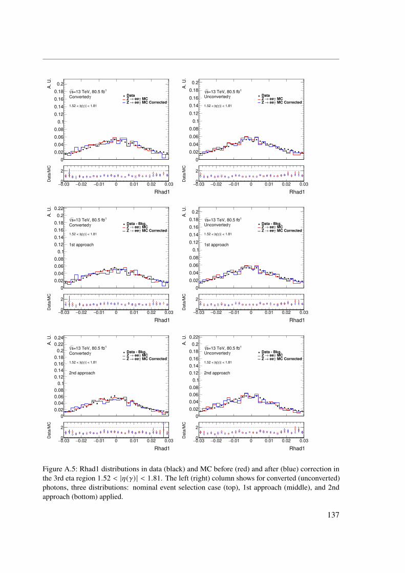
0
0.02
0.04
0.06
0.08
0.1
0.12
0.14
0.16
0.18
0.2
A.
U.
)| < 1.81γ(η1.52 < |
γConverted
-1=13 TeV, 80.5 fbs Data
MCγ ee→ Z MC Correctedγ ee→ Z
0.03− 0.02− 0.01− 0 0.01 0.02 0.03
Rhad1
0
2
Data
/MC
0
0.02
0.04
0.06
0.08
0.1
0.12
0.14
0.16
0.18
0.2
A.
U.
)| < 1.81γ(η1.52 < |
γUnconverted
-1=13 TeV, 80.5 fbs Data
MCγ ee→ Z MC Correctedγ ee→ Z
0.03− 0.02− 0.01− 0 0.01 0.02 0.03
Rhad1
0
2
Data
/MC
0
0.02
0.04
0.06
0.08
0.1
0.12
0.14
0.16
0.18
0.2
0.22
A.
U.
)| < 1.81γ(η1.52 < |
γConverted
-1=13 TeV, 80.5 fbs
1st approach
Data - Bkg. MCγ ee→ Z MC Correctedγ ee→ Z
0.03− 0.02− 0.01− 0 0.01 0.02 0.03
Rhad1
0
2
Data
/MC
0
0.02
0.04
0.06
0.08
0.1
0.12
0.14
0.16
0.18
0.2
A.
U.
)| < 1.81γ(η1.52 < |
γUnconverted
-1=13 TeV, 80.5 fbs
1st approach
Data - Bkg. MCγ ee→ Z MC Correctedγ ee→ Z
0.03− 0.02− 0.01− 0 0.01 0.02 0.03
Rhad1
0
2
Data
/MC
0
0.02
0.04
0.06
0.08
0.1
0.12
0.14
0.16
0.18
0.2
0.22
0.24
A.
U.
)| < 1.81γ(η1.52 < |
γConverted
-1=13 TeV, 80.5 fbs
2nd approach
Data - Bkg. MCγ ee→ Z MC Correctedγ ee→ Z
0.03− 0.02− 0.01− 0 0.01 0.02 0.03
Rhad1
0
2
Data
/MC
0
0.02
0.04
0.06
0.08
0.1
0.12
0.14
0.16
0.18
0.2
0.22
A.
U.
)| < 1.81γ(η1.52 < |
γUnconverted
-1=13 TeV, 80.5 fbs
2nd approach
Data - Bkg. MCγ ee→ Z MC Correctedγ ee→ Z
0.03− 0.02− 0.01− 0 0.01 0.02 0.03
Rhad1
0
2
Data
/MC
Figure A.5: Rhad1 distributions in data (black) and MC before (red) and after (blue) correction inthe 3rd eta region 1.52 < |�휂(�훾) | < 1.81. The left (right) column shows for converted (unconverted)photons, three distributions: nominal event selection case (top), 1st approach (middle), and 2ndapproach (bottom) applied.
137

Appendix A Additional shower shapes and fit results
0
0.02
0.04
0.06
0.08
0.1
0.12
0.14
0.16
0.18
0.2
0.22
A.
U.
)| < 2.37γ(η1.81 < |
γConverted
-1=13 TeV, 80.5 fbs Data
MCγ ee→ Z MC Correctedγ ee→ Z
0.03− 0.02− 0.01− 0 0.01 0.02 0.03
Rhad1
0
2
Data
/MC
0
0.02
0.04
0.06
0.08
0.1
0.12
0.14
0.16
0.18
0.2
0.22
A.
U.
)| < 2.37γ(η1.81 < |
γUnconverted
-1=13 TeV, 80.5 fbs Data
MCγ ee→ Z MC Correctedγ ee→ Z
0.03− 0.02− 0.01− 0 0.01 0.02 0.03
Rhad1
0
2
Data
/MC
0
0.02
0.04
0.06
0.08
0.1
0.12
0.14
0.16
0.18
0.2
0.22A.
U.
)| < 2.37γ(η1.81 < |
γConverted
-1=13 TeV, 80.5 fbs
1st approach
Data - Bkg. MCγ ee→ Z MC Correctedγ ee→ Z
0.03− 0.02− 0.01− 0 0.01 0.02 0.03
Rhad1
0
2
Data
/MC
0
0.02
0.04
0.06
0.08
0.1
0.12
0.14
0.16
0.18
0.2
0.22A
. U
.
)| < 2.37γ(η1.81 < |
γUnconverted
-1=13 TeV, 80.5 fbs
1st approach
Data - Bkg. MCγ ee→ Z MC Correctedγ ee→ Z
0.03− 0.02− 0.01− 0 0.01 0.02 0.03
Rhad1
0
2
Data
/MC
0
0.05
0.1
0.15
0.2
0.25
A.
U.
)| < 2.37γ(η1.81 < |
γConverted
-1=13 TeV, 80.5 fbs
2nd approach
Data - Bkg. MCγ ee→ Z MC Correctedγ ee→ Z
0.03− 0.02− 0.01− 0 0.01 0.02 0.03
Rhad1
0
2
Data
/MC
0
0.02
0.04
0.06
0.08
0.1
0.12
0.14
0.16
0.18
0.2
0.22
0.24
A.
U.
)| < 2.37γ(η1.81 < |
γUnconverted
-1=13 TeV, 80.5 fbs
2nd approach
Data - Bkg. MCγ ee→ Z MC Correctedγ ee→ Z
0.03− 0.02− 0.01− 0 0.01 0.02 0.03
Rhad1
0
2
Data
/MC
Figure A.6: Rhad1 distributions in data (black) and MC before (red) and after (blue) correction inthe 4th eta region 1.81 < |�휂(�훾) | < 2.37. The left (right) column shows for converted (unconverted)photons, three distributions: nominal event selection case (top), 1st approach (middle), and 2ndapproach (bottom) applied.
138

0
0.05
0.1
0.15
0.2
0.25
0.3A.
U.
)| < 0.6γ(η0 < |
γConverted
-1=13 TeV, 80.5 fbs Data
MCγ ee→ Z MC Correctedγ ee→ Z
0 0.1 0.2 0.3 0.4 0.5 0.6
f1
0
2
Data
/MC
0
0.05
0.1
0.15
0.2
0.25A.
U.
)| < 0.6γ(η0 < |
γUnconverted
-1=13 TeV, 80.5 fbs Data
MCγ ee→ Z MC Correctedγ ee→ Z
0 0.1 0.2 0.3 0.4 0.5 0.6
f1
0
2
Data
/MC
0
0.05
0.1
0.15
0.2
0.25
0.3A.
U.
)| < 0.6γ(η0 < |
γConverted
-1=13 TeV, 80.5 fbs
1st approach
Data - Bkg. MCγ ee→ Z MC Correctedγ ee→ Z
0 0.1 0.2 0.3 0.4 0.5 0.6
f1
0
2
Data
/MC
0
0.05
0.1
0.15
0.2
0.25
A.
U.
)| < 0.6γ(η0 < |
γUnconverted
-1=13 TeV, 80.5 fbs
1st approach
Data - Bkg. MCγ ee→ Z MC Correctedγ ee→ Z
0 0.1 0.2 0.3 0.4 0.5 0.6
f1
0
2
Data
/MC
0
0.05
0.1
0.15
0.2
0.25
0.3A.
U.
)| < 0.6γ(η0 < |
γConverted
-1=13 TeV, 80.5 fbs
2nd approach
Data - Bkg. MCγ ee→ Z MC Correctedγ ee→ Z
0 0.1 0.2 0.3 0.4 0.5 0.6
f1
0
2
Data
/MC
0
0.05
0.1
0.15
0.2
0.25
A.
U.
)| < 0.6γ(η0 < |
γUnconverted
-1=13 TeV, 80.5 fbs
2nd approach
Data - Bkg. MCγ ee→ Z MC Correctedγ ee→ Z
0 0.1 0.2 0.3 0.4 0.5 0.6
f1
0
2
Data
/MC
Figure A.7: f1 distributions in data (black) and MC before (red) and after (blue) correction in the 1steta region 0 < |�휂(�훾) | < 0.6. The left (right) column shows for converted (unconverted) photons, threedistributions: nominal event selection case (top), 1st approach (middle), and 2nd approach (bottom)applied.
139

Appendix A Additional shower shapes and fit results
0
0.05
0.1
0.15
0.2
0.25
0.3
0.35
0.4
A.
U.
)| < 1.37γ(η0.6 < |
γConverted
-1=13 TeV, 80.5 fbs Data
MCγ ee→ Z MC Correctedγ ee→ Z
0 0.1 0.2 0.3 0.4 0.5 0.6
f1
0
2
Data
/MC
0
0.05
0.1
0.15
0.2
0.25
0.3A.
U.
)| < 1.37γ(η0.6 < |
γUnconverted
-1=13 TeV, 80.5 fbs Data
MCγ ee→ Z MC Correctedγ ee→ Z
0 0.1 0.2 0.3 0.4 0.5 0.6
f1
0
2
Data
/MC
0
0.05
0.1
0.15
0.2
0.25
0.3
0.35
0.4
0.45
A.
U.
)| < 1.37γ(η0.6 < |
γConverted
-1=13 TeV, 80.5 fbs
1st approach
Data - Bkg. MCγ ee→ Z MC Correctedγ ee→ Z
0 0.1 0.2 0.3 0.4 0.5 0.6
f1
0
2
Data
/MC
0
0.05
0.1
0.15
0.2
0.25
0.3A.
U.
)| < 1.37γ(η0.6 < |
γUnconverted
-1=13 TeV, 80.5 fbs
1st approach
Data - Bkg. MCγ ee→ Z MC Correctedγ ee→ Z
0 0.1 0.2 0.3 0.4 0.5 0.6
f1
0
2
Data
/MC
0
0.05
0.1
0.15
0.2
0.25
0.3
0.35
0.4
0.45
A.
U.
)| < 1.37γ(η0.6 < |
γConverted
-1=13 TeV, 80.5 fbs
2nd approach
Data - Bkg. MCγ ee→ Z MC Correctedγ ee→ Z
0 0.1 0.2 0.3 0.4 0.5 0.6
f1
0
2
Data
/MC
0
0.05
0.1
0.15
0.2
0.25
0.3A.
U.
)| < 1.37γ(η0.6 < |
γUnconverted
-1=13 TeV, 80.5 fbs
2nd approach
Data - Bkg. MCγ ee→ Z MC Correctedγ ee→ Z
0 0.1 0.2 0.3 0.4 0.5 0.6
f1
0
2
Data
/MC
Figure A.8: f1 distributions in data (black) and MC before (red) and after (blue) correction in the 2ndeta region 0.6 < |�휂(�훾) | < 1.37. The left (right) column shows for converted (unconverted) photons,three distributions: nominal event selection case (top), 1st approach (middle), and 2nd approach(bottom) applied.
140

0
0.1
0.2
0.3
0.4
0.5A.
U.
)| < 1.81γ(η1.52 < |
γConverted
-1=13 TeV, 80.5 fbs Data
MCγ ee→ Z MC Correctedγ ee→ Z
0 0.1 0.2 0.3 0.4 0.5 0.6
f1
0
2
Data
/MC
0
0.05
0.1
0.15
0.2
0.25
0.3
0.35A.
U.
)| < 1.81γ(η1.52 < |
γUnconverted
-1=13 TeV, 80.5 fbs Data
MCγ ee→ Z MC Correctedγ ee→ Z
0 0.1 0.2 0.3 0.4 0.5 0.6
f1
0
2
Data
/MC
0
0.1
0.2
0.3
0.4
0.5A.
U.
)| < 1.81γ(η1.52 < |
γConverted
-1=13 TeV, 80.5 fbs
1st approach
Data - Bkg. MCγ ee→ Z MC Correctedγ ee→ Z
0 0.1 0.2 0.3 0.4 0.5 0.6
f1
0
2
Data
/MC
0
0.05
0.1
0.15
0.2
0.25
0.3
0.35A.
U.
)| < 1.81γ(η1.52 < |
γUnconverted
-1=13 TeV, 80.5 fbs
1st approach
Data - Bkg. MCγ ee→ Z MC Correctedγ ee→ Z
0 0.1 0.2 0.3 0.4 0.5 0.6
f1
0
2
Data
/MC
0
0.1
0.2
0.3
0.4
0.5
A.
U.
)| < 1.81γ(η1.52 < |
γConverted
-1=13 TeV, 80.5 fbs
2nd approach
Data - Bkg. MCγ ee→ Z MC Correctedγ ee→ Z
0 0.1 0.2 0.3 0.4 0.5 0.6
f1
0
2
Data
/MC
0
0.05
0.1
0.15
0.2
0.25
0.3
0.35
A.
U.
)| < 1.81γ(η1.52 < |
γUnconverted
-1=13 TeV, 80.5 fbs
2nd approach
Data - Bkg. MCγ ee→ Z MC Correctedγ ee→ Z
0 0.1 0.2 0.3 0.4 0.5 0.6
f1
0
2
Data
/MC
Figure A.9: f1 distributions in data (black) and MC before (red) and after (blue) correction in the 3rdeta region 1.52 < |�휂(�훾) | < 1.81. The left (right) column shows for converted (unconverted) photons,three distributions: nominal event selection case (top), 1st approach (middle), and 2nd approach(bottom) applied.
141

Appendix A Additional shower shapes and fit results
0
0.05
0.1
0.15
0.2
0.25
0.3A.
U.
)| < 2.37γ(η1.81 < |
γConverted
-1=13 TeV, 80.5 fbs Data
MCγ ee→ Z MC Correctedγ ee→ Z
0 0.1 0.2 0.3 0.4 0.5 0.6
f1
0
2
Data
/MC
0
0.05
0.1
0.15
0.2
0.25
A.
U.
)| < 2.37γ(η1.81 < |
γUnconverted
-1=13 TeV, 80.5 fbs Data
MCγ ee→ Z MC Correctedγ ee→ Z
0 0.1 0.2 0.3 0.4 0.5 0.6
f1
0
2
Data
/MC
0
0.05
0.1
0.15
0.2
0.25
0.3A.
U.
)| < 2.37γ(η1.81 < |
γConverted
-1=13 TeV, 80.5 fbs
1st approach
Data - Bkg. MCγ ee→ Z MC Correctedγ ee→ Z
0 0.1 0.2 0.3 0.4 0.5 0.6
f1
0
2
Data
/MC
0
0.05
0.1
0.15
0.2
0.25A
. U
.
)| < 2.37γ(η1.81 < |
γUnconverted
-1=13 TeV, 80.5 fbs
1st approach
Data - Bkg. MCγ ee→ Z MC Correctedγ ee→ Z
0 0.1 0.2 0.3 0.4 0.5 0.6
f1
0
2
Data
/MC
0
0.05
0.1
0.15
0.2
0.25
0.3
A.
U.
)| < 2.37γ(η1.81 < |
γConverted
-1=13 TeV, 80.5 fbs
2nd approach
Data - Bkg. MCγ ee→ Z MC Correctedγ ee→ Z
0 0.1 0.2 0.3 0.4 0.5 0.6
f1
0
2
Data
/MC
0
0.05
0.1
0.15
0.2
0.25
A.
U.
)| < 2.37γ(η1.81 < |
γUnconverted
-1=13 TeV, 80.5 fbs
2nd approach
Data - Bkg. MCγ ee→ Z MC Correctedγ ee→ Z
0 0.1 0.2 0.3 0.4 0.5 0.6
f1
0
2
Data
/MC
Figure A.10: f1 distributions in data (black) and MC before (red) and after (blue) correction in the 4theta region 1.81 < |�휂(�훾) | < 2.37. The left (right) column shows for converted (unconverted) photons,three distributions: nominal event selection case (top), 1st approach (middle), and 2nd approach(bottom) applied.
142

0
0.05
0.1
0.15
0.2
0.25
0.3
0.35A.
U.
)| < 0.6γ(η0 < |
γConverted
-1=13 TeV, 80.5 fbs Data
MCγ ee→ Z MC Correctedγ ee→ Z
0.6 0.65 0.7 0.75 0.8 0.85 0.9 0.95 1 1.05 1.1
Eratio
0
2
Data
/MC
0
0.05
0.1
0.15
0.2
0.25
0.3
0.35
0.4A.
U.
)| < 0.6γ(η0 < |
γUnconverted
-1=13 TeV, 80.5 fbs Data
MCγ ee→ Z MC Correctedγ ee→ Z
0.6 0.65 0.7 0.75 0.8 0.85 0.9 0.95 1 1.05 1.1
Eratio
0
2
Data
/MC
0
0.05
0.1
0.15
0.2
0.25
0.3
0.35
0.4A.
U.
)| < 0.6γ(η0 < |
γConverted
-1=13 TeV, 80.5 fbs
1st approach
Data - Bkg. MCγ ee→ Z MC Correctedγ ee→ Z
0.6 0.65 0.7 0.75 0.8 0.85 0.9 0.95 1 1.05 1.1
Eratio
0
2
Data
/MC
0
0.05
0.1
0.15
0.2
0.25
0.3
0.35
0.4
0.45
A.
U.
)| < 0.6γ(η0 < |
γUnconverted
-1=13 TeV, 80.5 fbs
1st approach
Data - Bkg. MCγ ee→ Z MC Correctedγ ee→ Z
0.6 0.65 0.7 0.75 0.8 0.85 0.9 0.95 1 1.05 1.1
Eratio
0
2
Data
/MC
0
0.1
0.2
0.3
0.4
0.5
A.
U.
)| < 0.6γ(η0 < |
γConverted
-1=13 TeV, 80.5 fbs
2nd approach
Data - Bkg. MCγ ee→ Z MC Correctedγ ee→ Z
0.6 0.65 0.7 0.75 0.8 0.85 0.9 0.95 1 1.05 1.1
Eratio
0
2
Data
/MC
0
0.1
0.2
0.3
0.4
0.5A.
U.
)| < 0.6γ(η0 < |
γUnconverted
-1=13 TeV, 80.5 fbs
2nd approach
Data - Bkg. MCγ ee→ Z MC Correctedγ ee→ Z
0.6 0.65 0.7 0.75 0.8 0.85 0.9 0.95 1 1.05 1.1
Eratio
0
2
Data
/MC
Figure A.11: Eratio distributions in data (black) and MC before (red) and after (blue) correction in the1st eta region 0 < |�휂(�훾) | < 0.6. The left (right) column shows for converted (unconverted) photons,three distributions: nominal event selection case (top), 1st approach (middle), and 2nd approach(bottom) applied.
143
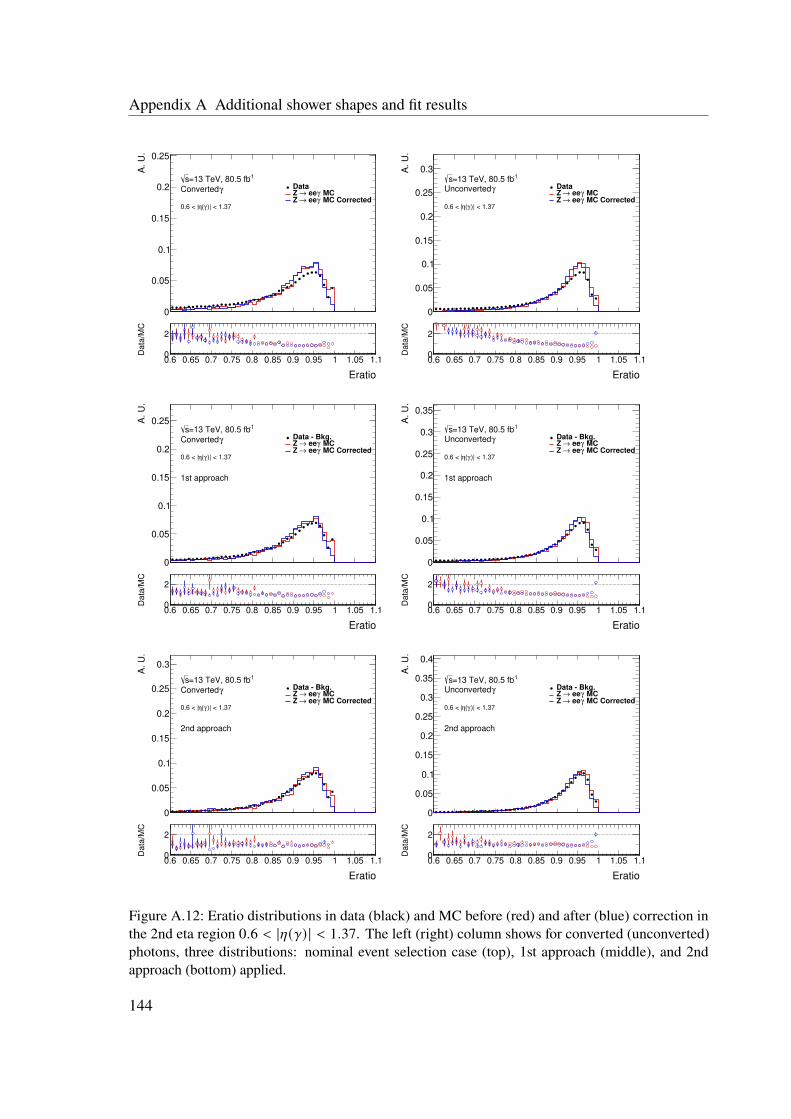
Appendix A Additional shower shapes and fit results
0
0.05
0.1
0.15
0.2
0.25
A.
U.
)| < 1.37γ(η0.6 < |
γConverted
-1=13 TeV, 80.5 fbs Data
MCγ ee→ Z MC Correctedγ ee→ Z
0.6 0.65 0.7 0.75 0.8 0.85 0.9 0.95 1 1.05 1.1
Eratio
0
2
Data
/MC
0
0.05
0.1
0.15
0.2
0.25
0.3A.
U.
)| < 1.37γ(η0.6 < |
γUnconverted
-1=13 TeV, 80.5 fbs Data
MCγ ee→ Z MC Correctedγ ee→ Z
0.6 0.65 0.7 0.75 0.8 0.85 0.9 0.95 1 1.05 1.1
Eratio
0
2
Data
/MC
0
0.05
0.1
0.15
0.2
0.25A.
U.
)| < 1.37γ(η0.6 < |
γConverted
-1=13 TeV, 80.5 fbs
1st approach
Data - Bkg. MCγ ee→ Z MC Correctedγ ee→ Z
0.6 0.65 0.7 0.75 0.8 0.85 0.9 0.95 1 1.05 1.1
Eratio
0
2
Data
/MC
0
0.05
0.1
0.15
0.2
0.25
0.3
0.35A
. U
.
)| < 1.37γ(η0.6 < |
γUnconverted
-1=13 TeV, 80.5 fbs
1st approach
Data - Bkg. MCγ ee→ Z MC Correctedγ ee→ Z
0.6 0.65 0.7 0.75 0.8 0.85 0.9 0.95 1 1.05 1.1
Eratio
0
2
Data
/MC
0
0.05
0.1
0.15
0.2
0.25
0.3
A.
U.
)| < 1.37γ(η0.6 < |
γConverted
-1=13 TeV, 80.5 fbs
2nd approach
Data - Bkg. MCγ ee→ Z MC Correctedγ ee→ Z
0.6 0.65 0.7 0.75 0.8 0.85 0.9 0.95 1 1.05 1.1
Eratio
0
2
Data
/MC
0
0.05
0.1
0.15
0.2
0.25
0.3
0.35
0.4
A.
U.
)| < 1.37γ(η0.6 < |
γUnconverted
-1=13 TeV, 80.5 fbs
2nd approach
Data - Bkg. MCγ ee→ Z MC Correctedγ ee→ Z
0.6 0.65 0.7 0.75 0.8 0.85 0.9 0.95 1 1.05 1.1
Eratio
0
2
Data
/MC
Figure A.12: Eratio distributions in data (black) and MC before (red) and after (blue) correction inthe 2nd eta region 0.6 < |�휂(�훾) | < 1.37. The left (right) column shows for converted (unconverted)photons, three distributions: nominal event selection case (top), 1st approach (middle), and 2ndapproach (bottom) applied.
144

0
0.05
0.1
0.15
0.2
0.25
A.
U.
)| < 1.81γ(η1.52 < |
γConverted
-1=13 TeV, 80.5 fbs Data
MCγ ee→ Z MC Correctedγ ee→ Z
0.6 0.65 0.7 0.75 0.8 0.85 0.9 0.95 1 1.05 1.1
Eratio
0
2
Data
/MC
0
0.05
0.1
0.15
0.2
0.25
0.3
0.35
0.4
A.
U.
)| < 1.81γ(η1.52 < |
γUnconverted
-1=13 TeV, 80.5 fbs Data
MCγ ee→ Z MC Correctedγ ee→ Z
0.6 0.65 0.7 0.75 0.8 0.85 0.9 0.95 1 1.05 1.1
Eratio
0
2
Data
/MC
0
0.05
0.1
0.15
0.2
0.25
0.3A.
U.
)| < 1.81γ(η1.52 < |
γConverted
-1=13 TeV, 80.5 fbs
1st approach
Data - Bkg. MCγ ee→ Z MC Correctedγ ee→ Z
0.6 0.65 0.7 0.75 0.8 0.85 0.9 0.95 1 1.05 1.1
Eratio
0
2
Data
/MC
0
0.05
0.1
0.15
0.2
0.25
0.3
0.35
0.4
0.45
A.
U.
)| < 1.81γ(η1.52 < |
γUnconverted
-1=13 TeV, 80.5 fbs
1st approach
Data - Bkg. MCγ ee→ Z MC Correctedγ ee→ Z
0.6 0.65 0.7 0.75 0.8 0.85 0.9 0.95 1 1.05 1.1
Eratio
0
2
Data
/MC
0
0.05
0.1
0.15
0.2
0.25
0.3
0.35A.
U.
)| < 1.81γ(η1.52 < |
γConverted
-1=13 TeV, 80.5 fbs
2nd approach
Data - Bkg. MCγ ee→ Z MC Correctedγ ee→ Z
0.6 0.65 0.7 0.75 0.8 0.85 0.9 0.95 1 1.05 1.1
Eratio
0
2
Data
/MC
0
0.1
0.2
0.3
0.4
0.5A.
U.
)| < 1.81γ(η1.52 < |
γUnconverted
-1=13 TeV, 80.5 fbs
2nd approach
Data - Bkg. MCγ ee→ Z MC Correctedγ ee→ Z
0.6 0.65 0.7 0.75 0.8 0.85 0.9 0.95 1 1.05 1.1
Eratio
0
2
Data
/MC
Figure A.13: Eratio distributions in data (black) and MC before (red) and after (blue) correction inthe 3rd eta region 1.52 < |�휂(�훾) | < 1.81. The left (right) column shows for converted (unconverted)photons, three distributions: nominal event selection case (top), 1st approach (middle), and 2ndapproach (bottom) applied.
145

Appendix A Additional shower shapes and fit results
0
0.1
0.2
0.3
0.4
0.5
0.6
0.7
0.8
0.9
A.
U.
)| < 2.37γ(η1.81 < |
γConverted
-1=13 TeV, 80.5 fbs Data
MCγ ee→ Z MC Correctedγ ee→ Z
0.6 0.65 0.7 0.75 0.8 0.85 0.9 0.95 1 1.05 1.1
Eratio
0
2
Data
/MC
0
0.1
0.2
0.3
0.4
0.5
0.6A.
U.
)| < 2.37γ(η1.81 < |
γUnconverted
-1=13 TeV, 80.5 fbs Data
MCγ ee→ Z MC Correctedγ ee→ Z
0.6 0.65 0.7 0.75 0.8 0.85 0.9 0.95 1 1.05 1.1
Eratio
0
2
Data
/MC
0
0.1
0.2
0.3
0.4
0.5
0.6
0.7
0.8
0.9
A.
U.
)| < 2.37γ(η1.81 < |
γConverted
-1=13 TeV, 80.5 fbs
1st approach
Data - Bkg. MCγ ee→ Z MC Correctedγ ee→ Z
0.6 0.65 0.7 0.75 0.8 0.85 0.9 0.95 1 1.05 1.1
Eratio
0
2
Data
/MC
0
0.1
0.2
0.3
0.4
0.5
0.6A.
U.
)| < 2.37γ(η1.81 < |
γUnconverted
-1=13 TeV, 80.5 fbs
1st approach
Data - Bkg. MCγ ee→ Z MC Correctedγ ee→ Z
0.6 0.65 0.7 0.75 0.8 0.85 0.9 0.95 1 1.05 1.1
Eratio
0
2
Data
/MC
0
0.1
0.2
0.3
0.4
0.5
0.6
0.7
0.8
0.9A.
U.
)| < 2.37γ(η1.81 < |
γConverted
-1=13 TeV, 80.5 fbs
2nd approach
Data - Bkg. MCγ ee→ Z MC Correctedγ ee→ Z
0.6 0.65 0.7 0.75 0.8 0.85 0.9 0.95 1 1.05 1.1
Eratio
0
2
Data
/MC
0
0.1
0.2
0.3
0.4
0.5
0.6A.
U.
)| < 2.37γ(η1.81 < |
γUnconverted
-1=13 TeV, 80.5 fbs
2nd approach
Data - Bkg. MCγ ee→ Z MC Correctedγ ee→ Z
0.6 0.65 0.7 0.75 0.8 0.85 0.9 0.95 1 1.05 1.1
Eratio
0
2
Data
/MC
Figure A.14: Eratio distributions in data (black) and MC before (red) and after (blue) correction inthe 4th eta region 1.81 < |�휂(�훾) | < 2.37. The left (right) column shows for converted (unconverted)photons, three distributions: nominal event selection case (top), 1st approach (middle), and 2ndapproach (bottom) applied.
146

0
0.1
0.2
0.3
0.4
0.5
0.6A.
U.
)| < 0.6γ(η0 < |
γConverted
-1=13 TeV, 80.5 fbs Data
MCγ ee→ Z MC Correctedγ ee→ Z
100− 50− 0 50 100 150 200 250 300
DeltaE
0
2
Data
/MC
0
0.1
0.2
0.3
0.4
0.5
0.6
A.
U.
)| < 0.6γ(η0 < |
γUnconverted
-1=13 TeV, 80.5 fbs Data
MCγ ee→ Z MC Correctedγ ee→ Z
100− 50− 0 50 100 150 200 250 300
DeltaE
0
2
Data
/MC
0
0.1
0.2
0.3
0.4
0.5
0.6
0.7A.
U.
)| < 0.6γ(η0 < |
γConverted
-1=13 TeV, 80.5 fbs
1st approach
Data - Bkg. MCγ ee→ Z MC Correctedγ ee→ Z
100− 50− 0 50 100 150 200 250 300
DeltaE
0
2
Data
/MC
0
0.1
0.2
0.3
0.4
0.5
0.6A.
U.
)| < 0.6γ(η0 < |
γUnconverted
-1=13 TeV, 80.5 fbs
1st approach
Data - Bkg. MCγ ee→ Z MC Correctedγ ee→ Z
100− 50− 0 50 100 150 200 250 300
DeltaE
0
2
Data
/MC
0
0.1
0.2
0.3
0.4
0.5
0.6
0.7
0.8
A.
U.
)| < 0.6γ(η0 < |
γConverted
-1=13 TeV, 80.5 fbs
2nd approach
Data - Bkg. MCγ ee→ Z MC Correctedγ ee→ Z
100− 50− 0 50 100 150 200 250 300
DeltaE
0
2
Data
/MC
0
0.1
0.2
0.3
0.4
0.5
0.6
0.7
A.
U.
)| < 0.6γ(η0 < |
γUnconverted
-1=13 TeV, 80.5 fbs
2nd approach
Data - Bkg. MCγ ee→ Z MC Correctedγ ee→ Z
100− 50− 0 50 100 150 200 250 300
DeltaE
0
2
Data
/MC
Figure A.15: DeltaE distributions in data (black) and MC before (red) and after (blue) correction in the1st eta region 0 < |�휂(�훾) | < 0.6. The left (right) column shows for converted (unconverted) photons,three distributions: nominal event selection case (top), 1st approach (middle), and 2nd approach(bottom) applied.
147

Appendix A Additional shower shapes and fit results
0
0.1
0.2
0.3
0.4
0.5
0.6
0.7A.
U.
)| < 1.37γ(η0.6 < |
γConverted
-1=13 TeV, 80.5 fbs Data
MCγ ee→ Z MC Correctedγ ee→ Z
100− 50− 0 50 100 150 200 250 300
DeltaE
0
2
Data
/MC
0
0.1
0.2
0.3
0.4
0.5
0.6
0.7
A.
U.
)| < 1.37γ(η0.6 < |
γUnconverted
-1=13 TeV, 80.5 fbs Data
MCγ ee→ Z MC Correctedγ ee→ Z
100− 50− 0 50 100 150 200 250 300
DeltaE
0
2
Data
/MC
0
0.1
0.2
0.3
0.4
0.5
0.6
0.7
0.8A.
U.
)| < 1.37γ(η0.6 < |
γConverted
-1=13 TeV, 80.5 fbs
1st approach
Data - Bkg. MCγ ee→ Z MC Correctedγ ee→ Z
100− 50− 0 50 100 150 200 250 300
DeltaE
0
2
Data
/MC
0
0.1
0.2
0.3
0.4
0.5
0.6
0.7A.
U.
)| < 1.37γ(η0.6 < |
γUnconverted
-1=13 TeV, 80.5 fbs
1st approach
Data - Bkg. MCγ ee→ Z MC Correctedγ ee→ Z
100− 50− 0 50 100 150 200 250 300
DeltaE
0
2
Data
/MC
0
0.1
0.2
0.3
0.4
0.5
0.6
0.7
0.8
0.9A.
U.
)| < 1.37γ(η0.6 < |
γConverted
-1=13 TeV, 80.5 fbs
2nd approach
Data - Bkg. MCγ ee→ Z MC Correctedγ ee→ Z
100− 50− 0 50 100 150 200 250 300
DeltaE
0
2
Data
/MC
0
0.1
0.2
0.3
0.4
0.5
0.6
0.7
0.8A.
U.
)| < 1.37γ(η0.6 < |
γUnconverted
-1=13 TeV, 80.5 fbs
2nd approach
Data - Bkg. MCγ ee→ Z MC Correctedγ ee→ Z
100− 50− 0 50 100 150 200 250 300
DeltaE
0
2
Data
/MC
Figure A.16: DeltaE distributions in data (black) and MC before (red) and after (blue) correction inthe 2nd eta region 0.6 < |�휂(�훾) | < 1.37. The left (right) column shows for converted (unconverted)photons, three distributions: nominal event selection case (top), 1st approach (middle), and 2ndapproach (bottom) applied.
148

0
0.1
0.2
0.3
0.4
0.5A.
U.
)| < 1.81γ(η1.52 < |
γConverted
-1=13 TeV, 80.5 fbs Data
MCγ ee→ Z MC Correctedγ ee→ Z
100− 50− 0 50 100 150 200 250 300
DeltaE
0
2
Data
/MC
0
0.1
0.2
0.3
0.4
0.5
A.
U.
)| < 1.81γ(η1.52 < |
γUnconverted
-1=13 TeV, 80.5 fbs Data
MCγ ee→ Z MC Correctedγ ee→ Z
100− 50− 0 50 100 150 200 250 300
DeltaE
0
2
Data
/MC
0
0.1
0.2
0.3
0.4
0.5
A.
U.
)| < 1.81γ(η1.52 < |
γConverted
-1=13 TeV, 80.5 fbs
1st approach
Data - Bkg. MCγ ee→ Z MC Correctedγ ee→ Z
100− 50− 0 50 100 150 200 250 300
DeltaE
0
2
Data
/MC
0
0.1
0.2
0.3
0.4
0.5A.
U.
)| < 1.81γ(η1.52 < |
γUnconverted
-1=13 TeV, 80.5 fbs
1st approach
Data - Bkg. MCγ ee→ Z MC Correctedγ ee→ Z
100− 50− 0 50 100 150 200 250 300
DeltaE
0
2
Data
/MC
0
0.1
0.2
0.3
0.4
0.5
0.6
A.
U.
)| < 1.81γ(η1.52 < |
γConverted
-1=13 TeV, 80.5 fbs
2nd approach
Data - Bkg. MCγ ee→ Z MC Correctedγ ee→ Z
100− 50− 0 50 100 150 200 250 300
DeltaE
0
2
Data
/MC
0
0.1
0.2
0.3
0.4
0.5A.
U.
)| < 1.81γ(η1.52 < |
γUnconverted
-1=13 TeV, 80.5 fbs
2nd approach
Data - Bkg. MCγ ee→ Z MC Correctedγ ee→ Z
100− 50− 0 50 100 150 200 250 300
DeltaE
0
2
Data
/MC
Figure A.17: DeltaE distributions in data (black) and MC before (red) and after (blue) correction inthe 3rd eta region 1.52 < |�휂(�훾) | < 1.81. The left (right) column shows for converted (unconverted)photons, three distributions: nominal event selection case (top), 1st approach (middle), and 2ndapproach (bottom) applied.
149

Appendix A Additional shower shapes and fit results
0
0.2
0.4
0.6
0.8
1A.
U.
)| < 2.37γ(η1.81 < |
γConverted
-1=13 TeV, 80.5 fbs Data
MCγ ee→ Z MC Correctedγ ee→ Z
100− 50− 0 50 100 150 200 250 300
DeltaE
0
2
Data
/MC
0
0.1
0.2
0.3
0.4
0.5
0.6
0.7A.
U.
)| < 2.37γ(η1.81 < |
γUnconverted
-1=13 TeV, 80.5 fbs Data
MCγ ee→ Z MC Correctedγ ee→ Z
100− 50− 0 50 100 150 200 250 300
DeltaE
0
2
Data
/MC
0
0.2
0.4
0.6
0.8
1A.
U.
)| < 2.37γ(η1.81 < |
γConverted
-1=13 TeV, 80.5 fbs
1st approach
Data - Bkg. MCγ ee→ Z MC Correctedγ ee→ Z
100− 50− 0 50 100 150 200 250 300
DeltaE
0
2
Data
/MC
0
0.1
0.2
0.3
0.4
0.5
0.6
0.7A.
U.
)| < 2.37γ(η1.81 < |
γUnconverted
-1=13 TeV, 80.5 fbs
1st approach
Data - Bkg. MCγ ee→ Z MC Correctedγ ee→ Z
100− 50− 0 50 100 150 200 250 300
DeltaE
0
2
Data
/MC
0
0.2
0.4
0.6
0.8
1A.
U.
)| < 2.37γ(η1.81 < |
γConverted
-1=13 TeV, 80.5 fbs
2nd approach
Data - Bkg. MCγ ee→ Z MC Correctedγ ee→ Z
100− 50− 0 50 100 150 200 250 300
DeltaE
0
2
Data
/MC
0
0.1
0.2
0.3
0.4
0.5
0.6
0.7A.
U.
)| < 2.37γ(η1.81 < |
γUnconverted
-1=13 TeV, 80.5 fbs
2nd approach
Data - Bkg. MCγ ee→ Z MC Correctedγ ee→ Z
100− 50− 0 50 100 150 200 250 300
DeltaE
0
2
Data
/MC
Figure A.18: DeltaE distributions in data (black) and MC before (red) and after (blue) correction inthe 4th eta region 1.81 < |�휂(�훾) | < 2.37. The left (right) column shows for converted (unconverted)photons, three distributions: nominal event selection case (top), 1st approach (middle), and 2ndapproach (bottom) applied.
150

APPENDIX B
Additional cross-section results
The full covariance matrices of the absolute cross-sections are shown in Tables B.1–B.5 andof the normalised ones are shown in Tables B.6–B.10.
Table B.1: Full covariance matrix of the absolute cross-section as a function of pT(�훾), accounting forstatistical and systematic uncertainties.
3.42e-02 7.26e-03 3.54e-03 2.44e-03 1.41e-03 9.95e-04 5.24e-04 3.20e-04 1.28e-04 4.19e-05 1.37e-057.26e-03 1.14e-02 2.14e-03 1.09e-03 6.80e-04 4.67e-04 2.60e-04 1.69e-04 6.49e-05 2.27e-05 8.39e-063.54e-03 2.14e-03 6.57e-03 1.06e-03 3.44e-04 2.61e-04 1.55e-04 9.45e-05 3.62e-05 1.22e-05 4.37e-062.44e-03 1.09e-03 1.06e-03 4.19e-03 5.33e-04 2.04e-04 1.28e-04 8.62e-05 3.30e-05 1.21e-05 4.00e-061.41e-03 6.80e-04 3.44e-04 5.33e-04 1.91e-03 2.20e-04 7.68e-05 5.32e-05 2.05e-05 7.67e-06 2.67e-069.95e-04 4.67e-04 2.61e-04 2.04e-04 2.20e-04 1.12e-03 7.83e-05 3.38e-05 1.38e-05 5.28e-06 1.79e-065.24e-04 2.60e-04 1.55e-04 1.28e-04 7.68e-05 7.83e-05 3.99e-04 2.71e-05 8.09e-06 3.08e-06 1.05e-063.20e-04 1.69e-04 9.45e-05 8.62e-05 5.32e-05 3.38e-05 2.71e-05 2.08e-04 7.49e-06 2.37e-06 8.79e-071.28e-04 6.49e-05 3.62e-05 3.30e-05 2.05e-05 1.38e-05 8.09e-06 7.49e-06 3.25e-05 1.09e-06 3.53e-074.19e-05 2.27e-05 1.22e-05 1.21e-05 7.67e-06 5.28e-06 3.08e-06 2.37e-06 1.09e-06 8.87e-06 1.56e-071.37e-05 8.39e-06 4.37e-06 4.00e-06 2.67e-06 1.79e-06 1.05e-06 8.79e-07 3.53e-07 1.56e-07 1.51e-06
Table B.2: Full covariance matrix of the absolute cross-section as a function of |�휂(�훾) |, accounting forstatistical and systematic uncertainties.
3.95e+00 5.05e-01 3.94e-01 4.18e-01 4.21e-01 3.89e-01 3.39e-01 2.17e-015.05e-01 3.83e+00 5.14e-01 4.07e-01 4.21e-01 3.98e-01 3.40e-01 2.15e-013.94e-01 5.14e-01 3.38e+00 4.80e-01 4.14e-01 4.06e-01 3.54e-01 2.23e-014.18e-01 4.07e-01 4.80e-01 3.69e+00 5.31e-01 4.41e-01 4.02e-01 2.56e-014.21e-01 4.21e-01 4.14e-01 5.31e-01 3.24e+00 5.73e-01 4.76e-01 3.12e-013.89e-01 3.98e-01 4.06e-01 4.41e-01 5.73e-01 2.70e+00 4.92e-01 3.07e-013.39e-01 3.40e-01 3.54e-01 4.02e-01 4.76e-01 4.92e-01 1.81e+00 3.06e-012.17e-01 2.15e-01 2.23e-01 2.56e-01 3.12e-01 3.07e-01 3.06e-01 6.07e-01
151

Appendix B Additional cross-section results
Table B.3: Full covariance matrix of the absolute cross-section as a function of Δ�푅(�훾, �푙)min, accountingfor statistical and systematic uncertainties.
8.18e+00 8.53e-01 5.64e-01 4.54e-01 3.64e-01 3.49e-01 3.37e-01 3.03e-01 1.62e-01 2.42e-028.53e-01 6.08e+00 6.13e-01 3.94e-01 3.12e-01 3.03e-01 3.03e-01 2.71e-01 1.44e-01 2.17e-025.64e-01 6.13e-01 4.96e+00 3.94e-01 2.63e-01 2.61e-01 2.69e-01 2.39e-01 1.40e-01 2.42e-024.54e-01 3.94e-01 3.94e-01 4.05e+00 3.51e-01 3.21e-01 2.98e-01 2.49e-01 1.81e-01 4.06e-023.64e-01 3.12e-01 2.63e-01 3.51e-01 2.15e+00 3.92e-01 3.35e-01 2.66e-01 2.24e-01 5.57e-023.49e-01 3.03e-01 2.61e-01 3.21e-01 3.92e-01 1.80e+00 3.46e-01 2.77e-01 2.29e-01 5.70e-023.37e-01 3.03e-01 2.69e-01 2.98e-01 3.35e-01 3.46e-01 1.84e+00 2.87e-01 2.26e-01 5.46e-023.03e-01 2.71e-01 2.39e-01 2.49e-01 2.66e-01 2.77e-01 2.87e-01 1.06e+00 1.99e-01 4.58e-021.62e-01 1.44e-01 1.40e-01 1.81e-01 2.24e-01 2.29e-01 2.26e-01 1.99e-01 6.77e-01 4.13e-022.42e-02 2.17e-02 2.42e-02 4.06e-02 5.57e-02 5.70e-02 5.46e-02 4.58e-02 4.13e-02 2.55e-02
Table B.4: Full covariance matrix of the absolute cross-section as a function of Δ�휙(�푙, �푙), accountingfor statistical and systematic uncertainties.
5.77e-01 1.34e-01 1.34e-01 1.41e-01 1.41e-01 1.63e-01 1.60e-01 1.80e-01 1.79e-01 2.06e-011.34e-01 7.08e-01 1.67e-01 1.74e-01 1.79e-01 2.10e-01 2.08e-01 2.30e-01 2.19e-01 2.66e-011.34e-01 1.67e-01 1.03e+00 1.89e-01 1.96e-01 2.27e-01 2.26e-01 2.49e-01 2.29e-01 2.70e-011.41e-01 1.74e-01 1.89e-01 1.61e+00 2.09e-01 2.39e-01 2.35e-01 2.63e-01 2.50e-01 2.88e-011.41e-01 1.79e-01 1.96e-01 2.09e-01 1.66e+00 2.57e-01 2.55e-01 2.87e-01 2.68e-01 3.13e-011.63e-01 2.10e-01 2.27e-01 2.39e-01 2.57e-01 2.66e+00 3.01e-01 3.43e-01 3.17e-01 3.88e-011.60e-01 2.08e-01 2.26e-01 2.35e-01 2.55e-01 3.01e-01 2.87e+00 3.33e-01 3.04e-01 3.78e-011.80e-01 2.30e-01 2.49e-01 2.63e-01 2.87e-01 3.43e-01 3.33e-01 2.78e+00 3.53e-01 4.23e-011.79e-01 2.19e-01 2.29e-01 2.50e-01 2.68e-01 3.17e-01 3.04e-01 3.53e-01 2.91e+00 4.04e-012.06e-01 2.66e-01 2.70e-01 2.88e-01 3.13e-01 3.88e-01 3.78e-01 4.23e-01 4.04e-01 4.56e+00
Table B.5: Full covariance matrix of the absolute cross-section as a function of |Δ�휂(�푙, �푙) |, accountingfor statistical and systematic uncertainties.
2.50e+00 4.66e-01 5.30e-01 4.28e-01 3.54e-01 2.97e-01 2.21e-01 4.21e-024.66e-01 2.17e+00 4.68e-01 3.77e-01 3.09e-01 2.64e-01 1.96e-01 3.72e-025.30e-01 4.68e-01 2.61e+00 4.35e-01 3.53e-01 2.96e-01 2.25e-01 4.20e-024.28e-01 3.77e-01 4.35e-01 2.06e+00 2.89e-01 2.42e-01 1.83e-01 3.50e-023.54e-01 3.09e-01 3.53e-01 2.89e-01 1.66e+00 1.98e-01 1.49e-01 2.85e-022.97e-01 2.64e-01 2.96e-01 2.42e-01 1.98e-01 1.40e+00 1.26e-01 2.44e-022.21e-01 1.96e-01 2.25e-01 1.83e-01 1.49e-01 1.26e-01 7.74e-01 1.86e-024.21e-02 3.72e-02 4.20e-02 3.50e-02 2.85e-02 2.44e-02 1.86e-02 2.66e-02
152

Table B.6: Full covariance matrix of the normalised cross-section as a function of pT(�훾), accountingfor statistical and systematic uncertainties.
1.36e-05 2.53e-07 -5.27e-07 -4.47e-07 -3.83e-07 -2.64e-07 -2.32e-07 -1.14e-07 -6.16e-08 -2.21e-08 -8.60e-092.53e-07 5.11e-06 8.37e-08 -1.83e-07 -1.13e-07 -8.44e-08 -5.64e-08 -2.68e-08 -1.48e-08 -4.60e-09 -1.40e-09-5.27e-07 8.37e-08 3.38e-06 1.79e-07 -7.28e-08 -3.76e-08 -1.88e-08 -9.50e-09 -5.00e-09 -1.20e-09 -2.00e-10-4.47e-07 -1.83e-07 1.79e-07 2.32e-06 1.56e-07 9.90e-09 1.27e-08 1.32e-08 4.10e-09 2.20e-09 1.10e-09-3.83e-07 -1.13e-07 -7.28e-08 1.56e-07 1.10e-06 6.71e-08 9.20e-09 7.80e-09 4.00e-09 1.80e-09 8.00e-10-2.64e-07 -8.44e-08 -3.76e-08 9.90e-09 6.71e-08 6.57e-07 2.37e-08 5.50e-09 2.70e-09 1.40e-09 6.00e-10-2.32e-07 -5.64e-08 -1.88e-08 1.27e-08 9.20e-09 2.37e-08 2.38e-07 8.80e-09 2.50e-09 1.20e-09 5.00e-10-1.14e-07 -2.68e-08 -9.50e-09 1.32e-08 7.80e-09 5.50e-09 8.80e-09 1.25e-07 2.40e-09 7.00e-10 4.00e-10-6.16e-08 -1.48e-08 -5.00e-09 4.10e-09 4.00e-09 2.70e-09 2.50e-09 2.40e-09 1.98e-08 5.00e-10 2.00e-10-2.21e-08 -4.60e-09 -1.20e-09 2.20e-09 1.80e-09 1.40e-09 1.20e-09 7.00e-10 5.00e-10 5.50e-09 1.00e-10-8.60e-09 -1.40e-09 -2.00e-10 1.10e-09 8.00e-10 6.00e-10 5.00e-10 4.00e-10 2.00e-10 1.00e-10 1.00e-09
Table B.7: Full covariance matrix of the normalised cross-section as a function of |�휂(�훾) |, accountingfor statistical and systematic uncertainties.
2.19e-03 3.83e-05 -3.69e-05 -6.47e-05 -8.36e-05 -5.51e-05 -2.33e-05 1.14e-053.83e-05 2.12e-03 4.06e-05 -6.28e-05 -7.43e-05 -4.83e-05 -1.09e-05 1.76e-05-3.69e-05 4.06e-05 1.83e-03 -1.39e-05 -7.36e-05 -4.90e-05 -1.51e-05 9.90e-06-6.47e-05 -6.28e-05 -1.39e-05 1.95e-03 -4.85e-05 -6.63e-05 -3.66e-05 -7.66e-06-8.36e-05 -7.43e-05 -7.36e-05 -4.85e-05 1.61e-03 -3.30e-05 -5.41e-05 -2.11e-05-5.51e-05 -4.83e-05 -4.90e-05 -6.63e-05 -3.30e-05 1.32e-03 -2.66e-05 -9.94e-06-2.33e-05 -1.09e-05 -1.51e-05 -3.66e-05 -5.41e-05 -2.66e-05 8.18e-04 8.01e-061.14e-05 1.76e-05 9.90e-06 -7.66e-06 -2.11e-05 -9.94e-06 8.01e-06 2.73e-04
Table B.8: Full covariance matrix of the normalised cross-section as a function of Δ�푅(�훾, �푙)min,accounting for statistical and systematic uncertainties.
4.88e-03 1.71e-04 2.55e-05 -5.91e-05 -1.50e-04 -1.38e-04 -6.78e-05 3.25e-05 5.92e-05 2.40e-051.71e-04 3.50e-03 7.16e-05 -5.96e-05 -1.22e-04 -1.12e-04 -6.00e-05 1.43e-05 2.89e-05 1.33e-052.55e-05 7.16e-05 2.89e-03 -6.81e-06 -9.81e-05 -8.54e-05 -4.97e-05 2.51e-06 1.57e-05 9.07e-06-5.91e-05 -5.96e-05 -6.81e-06 2.34e-03 -2.80e-05 -3.42e-05 -2.90e-05 -8.63e-06 1.43e-05 1.01e-05-1.50e-04 -1.22e-04 -9.81e-05 -2.80e-05 1.12e-03 7.21e-06 -1.65e-05 -2.21e-05 1.33e-05 1.12e-05-1.38e-04 -1.12e-04 -8.54e-05 -3.42e-05 7.21e-06 9.09e-04 -8.64e-06 -2.06e-05 9.72e-06 9.03e-06-6.78e-05 -6.00e-05 -4.97e-05 -2.90e-05 -1.65e-05 -8.64e-06 9.43e-04 -8.35e-06 1.25e-05 8.65e-063.25e-05 1.43e-05 2.51e-06 -8.63e-06 -2.21e-05 -2.06e-05 -8.35e-06 5.22e-04 2.16e-05 9.09e-065.92e-05 2.89e-05 1.57e-05 1.43e-05 1.33e-05 9.72e-06 1.25e-05 2.16e-05 3.61e-04 1.37e-052.40e-05 1.33e-05 9.07e-06 1.01e-05 1.12e-05 9.03e-06 8.65e-06 9.09e-06 1.37e-05 1.42e-05
153

Appendix B Additional cross-section results
Table B.9: Full covariance matrix of the normalised cross-section as a function of Δ�휙(�푙, �푙), accountingfor statistical and systematic uncertainties.
2.96e-04 1.16e-06 -9.46e-06 -1.71e-05 -2.28e-05 -2.60e-05 -3.16e-05 -2.79e-05 -2.79e-05 -2.80e-051.16e-06 3.38e-04 -1.35e-05 -2.13e-05 -2.55e-05 -2.72e-05 -3.19e-05 -3.08e-05 -3.26e-05 -3.09e-05-9.46e-06 -1.35e-05 5.13e-04 -2.64e-05 -3.25e-05 -3.60e-05 -4.09e-05 -4.05e-05 -4.43e-05 -4.84e-05-1.71e-05 -2.13e-05 -2.64e-05 8.50e-04 -3.53e-05 -4.14e-05 -4.42e-05 -4.35e-05 -4.29e-05 -4.33e-05-2.28e-05 -2.55e-05 -3.25e-05 -3.53e-05 8.62e-04 -3.77e-05 -3.95e-05 -4.17e-05 -4.22e-05 -3.49e-05-2.60e-05 -2.72e-05 -3.60e-05 -4.14e-05 -3.77e-05 1.43e-03 -3.89e-05 -4.41e-05 -4.95e-05 -3.65e-05-3.16e-05 -3.19e-05 -4.09e-05 -4.42e-05 -3.95e-05 -3.89e-05 1.57e-03 -4.59e-05 -4.83e-05 -3.33e-05-2.79e-05 -3.08e-05 -4.05e-05 -4.35e-05 -4.17e-05 -4.41e-05 -4.59e-05 1.45e-03 -4.58e-05 -4.05e-05-2.79e-05 -3.26e-05 -4.43e-05 -4.29e-05 -4.22e-05 -4.95e-05 -4.83e-05 -4.58e-05 1.57e-03 -2.99e-05-2.80e-05 -3.09e-05 -4.84e-05 -4.33e-05 -3.49e-05 -3.65e-05 -3.33e-05 -4.05e-05 -2.99e-05 2.50e-03
Table B.10: Full covariance matrix of the normalised cross-section as a function of |Δ�휂(�푙, �푙) |,accounting for statistical and systematic uncertainties.
1.18e-03 -7.62e-05 -8.68e-05 -7.71e-05 -6.12e-05 -4.76e-05 -3.88e-05 -9.19e-06-7.62e-05 1.05e-03 -6.63e-05 -5.89e-05 -5.22e-05 -4.18e-05 -3.09e-05 -6.45e-06-8.68e-05 -6.63e-05 1.24e-03 -6.58e-05 -5.88e-05 -4.75e-05 -3.42e-05 -7.69e-06-7.71e-05 -5.89e-05 -6.58e-05 1.03e-03 -4.96e-05 -4.02e-05 -2.85e-05 -6.19e-06-6.12e-05 -5.22e-05 -5.88e-05 -4.96e-05 8.63e-04 -3.34e-05 -2.40e-05 -5.33e-06-4.76e-05 -4.18e-05 -4.75e-05 -4.02e-05 -3.34e-05 7.56e-04 -1.94e-05 -4.24e-06-3.88e-05 -3.09e-05 -3.42e-05 -2.85e-05 -2.40e-05 -1.94e-05 4.15e-04 -2.90e-06-9.19e-06 -6.45e-06 -7.69e-06 -6.19e-06 -5.33e-06 -4.24e-06 -2.90e-06 1.40e-05
154