DISCUSSION PAPER SERIES

IZA DP No. 11379

José AzarIoana MarinescuMarshall SteinbaumBledi Taska

Concentration in US Labor Markets: Evidence from Online Vacancy Data

MARCH 2018

Any opinions expressed in this paper are those of the author(s) and not those of IZA. Research published in this series may include views on policy, but IZA takes no institutional policy positions. The IZA research network is committed to the IZA Guiding Principles of Research Integrity.The IZA Institute of Labor Economics is an independent economic research institute that conducts research in labor economics and offers evidence-based policy advice on labor market issues. Supported by the Deutsche Post Foundation, IZA runs the world’s largest network of economists, whose research aims to provide answers to the global labor market challenges of our time. Our key objective is to build bridges between academic research, policymakers and society.IZA Discussion Papers often represent preliminary work and are circulated to encourage discussion. Citation of such a paper should account for its provisional character. A revised version may be available directly from the author.

Schaumburg-Lippe-Straße 5–953113 Bonn, Germany

Phone: +49-228-3894-0Email: publications@iza.org www.iza.org

IZA – Institute of Labor Economics

DISCUSSION PAPER SERIES

IZA DP No. 11379

Concentration in US Labor Markets: Evidence from Online Vacancy Data

MARCH 2018

José AzarIESE Business School, Universidad de Navarra

Ioana MarinescuUniversity of Pennsylvania, NBER and IZA

Marshall SteinbaumRoosevelt Institute

Bledi TaskaBurning Glass Technologies

ABSTRACT

IZA DP No. 11379 MARCH 2018

Concentration in US Labor Markets: Evidence from Online Vacancy Data*

Using data on the near-universe of online US job vacancies collected by Burning Glass

Technologies in 2016, we calculate labor market concentration using the Herfindahl-

Hirschman index (HHI) for each commuting zone by 6-digit SOC occupation. The average

market has an HHI of 3,953, or the equivalent of 2.5 recruiting employers. 54% of labor

markets are highly concentrated (above 2,500 HHI) according to the DOJ/FTC guidelines.

Highly concentrated markets account for 17% of employment. All plausible alternative

market definitions show that more than 33% of markets are highly concentrated,

suggesting that employers have market power in many US labor markets.

JEL Classification: J21, J23, J42, K21, L11

Keywords: monopsony, oligopsony, labor markets, competition policy

Corresponding author:Ioana MarinescuSchool of Social Policy & PracticeUniversity of Pennsylvania3701 Locust WalkPhiladelphia PA, 19104-6214USA

E-mail: ioma@upenn.edu

* José Azar gratefully acknowledges the financial support of Secretaria d’Universitats I Recerca del Departament

d’Empresa I Coneixement de la Generalitat de Catalunya. Ref.2016 BP00358. Steinbaum acknowledges the support

of the Ewing Marion Kauffman Foundation.

1 Introduction

While interest in labor market monopsony power has increased in recent years (Ashenfel-

ter, Farber and Ransom, 2010; Manning, 2011; CEA, 2016), the effects of mergers and other

anti-competitive conduct on labor markets are generally not taken into account in antitrust

practice. Antitrust enforcement is based on the consumer welfare standard, i.e. examining the

adverse effects of anticompetitive behavior for consumers. This is despite substantial evidence

of market power in the labor market (Staiger, Spetz and Phibbs, 2010; Falch, 2010; Ransom and

Sims, 2010; Dube, Lester and Reich, 2016). But this empirical work has generally focused on

particular labor markets (e.g. Matsudaira, 2013), and there is little evidence to inform the de-

bate about how widespread labor market concentration is, and how it varies across occupations

and geographies in the US.

In this paper, we directly quantify the level of labor market concentration across nearly all

occupations and for every commuting zone in the US, building on our findings in Azar, Mari-

nescu and Steinbaum (2017). The earlier paper used data for the most frequent occupations

from a large online job board (CareerBuilder.com) to show that higher concentration is asso-

ciated with lower posted wages. Here, we focus on systematically measuring concentration.

We use a dataset from Burning Glass Technologies (BGT) covering the near-universe of online

US vacancy postings in 2016. This allows us to give a comprehensive picture of labor market

concentration in the US.

We calculate Herfindahl Hirschman Indices (HHIs) for labor markets at the occupation (6-

digit SOC), commuting zone and quarterly level. The average market has an HHI of 3953,

which is the equivalent of 2.5 recruiting firms. 54% of markets are highly concentrated (above

2,500 HHI) by the standard of the Department of Justice / Federal Trade Commission 2010

horizontal merger guidelines. To understand the threshold for high concentration, note that

a market with four firms and equal market shares has an HHI of 2,500, so an HHI of 2500 is

the equivalent of 4 recruiting firms. Another 11% of markets are moderately concentrated by

1

the standard of the Department of Justice / Federal Trade Commission 2010 horizontal merger

guidelines, i.e. have an HHI between 1,500 and 2,500. When we weight markets by BLS total

employment, we find that 17 percent of workers work in highly concentrated labor markets (by

our measure of concentration from Burning Glass), and a further 6 percent work in moderately

concentrated markets. Concentration is lower in large commuting zones, which explains why

weighing by employment lowers the prevalence of high concentration.

We carefully discuss the definition of a labor market, and provide a justification for our

choice of the 6-digit SOC by commuting zone by quarter; we also calculate concentration for a

number of alternative market definitions in terms of occupation, location and time. According

to all plausible alternative market definitions, we find that at least 33% of markets are highly

concentrated. Given the observed level of concentration, company mergers have the potential

to significantly increase employers’ labor market power. The labor market concentration mea-

sure we develop here can be usefully leveraged in merger reviews and the litigation of other

anti-competitive behaviors1 in the labor market, as detailed in Marinescu and Hovenkamp

(2018) and Naidu, Posner and Weyl (2018).

Our measure of concentration is distinct from the industry concentration measures used by

Autor et al. (2017) and Barkai (2016): it is based on concentration in the labor market rather

than concentration in the product market. Our contribution is therefore complementary, and it

is the first economy-wide measure of labor market concentration to have been made in many

decades.2

The recent study that comes closest to our approach is Benmelech, Bergman and Kim (2018),

which uses Census data for manufacturing industries over a long time horizon to measure em-

ployment concentration (as opposed to vacancy concentration) and its effect on wages. Those

authors focus on county-industries as the analogues to local labor markets, whereas we use

commuting zones and six-digit SOC occupations.

1Examples include no-poaching agreements (Ashenfelter and Krueger, 2017), and, in some cases, non-competition agreements (Starr, Prescott and Bishara, 2017).

2The last, to our knowledge, is Bunting (1962); see review of literature by Boal and Ransom (1997).

2

In contrast to Benmelech, Bergman and Kim (2018), we measure concentration using job

openings rather than employment because we view vacancies as a better gauge of how likely

searching workers (whether employed or unemployed) are to receive a job offer. Recent stud-

ies show that workers remain in jobs for longer.3 The corollary is that jobs are vacated less

frequently, and so the concentration of employment is a less relevant gauge of available work

and employer market power than is the concentration of vacancies among the relatively few

firms who are likely to be hiring at any given time.

Section 2 describes the Burning Glass data, section 3 addresses market definition for labor

markets, and section 4 gives our estimates of labor market concentration. Section 5 places

our results in the larger debate over inter-firm inequality compares concentration in the labor

market to concentration in the product market, and section 6 concludes.

2 Data

We use data from Burning Glass Technologies (BGT). The company examines about 40,000

websites and believes to be able to capture the near-universe of online US vacancies. Hersh-

bein and Kahn (2016); Deming and Kahn (2017); Modestino, Shoag and Ballance (2016) have

used this data and provide a more in-depth description. Importantly, BGT data is fairly similar

in terms of industry composition when compared to all vacancies recorded in the Job Open-

ings and Labor Turnover Survey (JOLTS) (Hershbein and Kahn, 2016). Furthermore, the oc-

cupational distribution is similar to the one found in the Occupational Employment Statistics

(Hershbein and Kahn, 2016).

We restrict the data to 2016 because this is the year with the highest data quality and the

greatest coverage for vacancies across the US. Indeed, the tools used by BGT improve over

time, and more and more of the US vacancies are online.4 To understand the share of job

openings captured by BGT, it is important to note BGT only measures new postings (the same

3See Haltiwanger et al. (forthcoming), Molloy et al. (2016), and Konczal and Steinbaum (2016).4Average concentration levels in 2007-2015 are comparable to average concentration levels in 2016.

3

posting appears only on the first month it is recorded) while JOLTS measures active postings

(the same posting can appear in two or more consecutive months if time to fill is more than

30 days). Help Wanted Online (HWOL) measures both. Therefore, the number of postings on

BGT can be inflated using the new jobs to active jobs ratio in HWOL, i.e. the same method used

in Carnevale, Jayasundera and Repnikov (2014). Based on this calculation, BGT shows that the

share of jobs online as captured by BGT is roughly 85% of the jobs in JOLTS in 2016. The jobs

that are not online now are usually in small businesses (the classic example being the “help

wanted” sign in the restaurant window) and union hiring halls. Overall, however, research

shows the online job market has consistently expanded over the last few years.

The data is cleaned by Burning Glass to remove vacancy duplicates and extract key charac-

teristics for each vacancy. Of interest to our work are the location of the vacancy (county), name

of the employer, and the occupation. The name of the employer is normalized by BGT so that

similar employer names are grouped together into a single employer: for example, “Bausch

and Lomb”, “Bausch Lomb”, and “Bausch & Lomb” would be grouped together. Still, 35.9% of

employer names are missing, partly due to staffing companies not disclosing which employer

the job is at. To calculate concentration, we will assume that all these missing employer names

are different, thus providing a lower bound for labor market concentration.

The BGT dataset contains many variables describing the occupation of each vacancy. These

include the SOC code, the standardized job title, and the BGT occupation. The standardized

job title is based on the full text job title of the job vacancy: the full text job title is cleaned

and similar job titles are grouped together. The BGT occupation starts with the SOC code, and

either consolidates SOC codes or divides them into several categories based on the similarity

of skills, education and knowledge requirements.

We drop internships and data with missing SOC or commuting zones, which represents

5.2% of the initial sample. We are left with a sample of 24,317,178 observations.

For our benchmark analysis, we keep 200 occupations, which represent 90% of vacancy

postings in the BGT dataset. We trim away very small occupations because they may be de-

4

fined too narrowly. We note that this choice results in lower HHI than if we had included all

occupations. The total number of markets (6-digit SOC occupation by commuting zone) we

consider in our main analysis is 117,707.

Our main summary statistics on HHI treat each cell (commuting zone by 6-dgit SOC by

quarter) as an observation. But we also want to understand how the summary statistics change

when we weight by employment in each of these markets. When we report HHI weighted by

employment, we include every occupation in the data, since small and possibly ill-defined

occupations will not be overly influential after weighing by employment. To analyze HHI

weighted by employment, we use the May 2016 Metropolitan and Nonmetropolitan Area Oc-

cupational Employment and Wage estimates from the Bureau of Labor Statistics (BLS). The

BLS data is only available at the CBSA level, and not at the commuting zone level. To get

commuting zone employment, we first estimate BLS county-level employment: we use county

population shares within a CBSA and multiply these shares with the BLS employment by 6-

digit SOC at the CBSA level. Finally, to get commuting zone 6-digit SOC employment numbers,

we aggregate the 6-digit SOC employment numbers across the counties that form a commuting

zone.

3 Herfindahl-Hirschman Index and Labor Market Definition

3.1 Herfindahl-Hirschman Index

Our baseline measure of concentration in a labor market is the Herfindahl-Hirschman In-

dex (HHI) calculated based on the share of vacancies of all the firms that post vacancies in

that market. The HHI is widely used as a measure of market concentration in the industrial

organization literature and in antitrust practice. An advantage of this measure of market con-

centration is that there are guidelines for what represents a high level of market concentration.

The DOJ/FTC guidelines: an HHI above 1500 is "moderately concentrated", and above 2500 is

5

"highly concentrated". Also, a merger that increases the HHI by more than 200 points, leading

to a highly concentrated market is "presumed likely to increase market power".

While these measures and thresholds are generally used to evaluate market concentration

in product markets, the antitrust agency guidelines state that “[t]o evaluate whether a merger

is likely to enhance market power on the buying side of the market, the Agencies employ

essentially the framework described above for evaluating whether a merger is likely to enhance

market power on the selling side of the market.” This implies that adverse effects of mergers on

the inputs market, including the labor market, are part of the legal framework for evaluating

mergers.

The formula for the HHI in market m and time t is

HHIm,t =J

∑j=1

s2j,m,t (3.1)

where sj,m is the market share of firm j in market m. The market share of a firm in a given

market and time is defined as the sum of vacancies posted by a given firm in a given market

and time divided by total vacancies posted in that market and time. The inverse of the HHI

multiplied by 10,000, 10,000/HHI, gives the “equivalent” number of firms in the market, or the

number of firms that would result in such an HHI if each had the same share of the market.

When reporting average HHI, we first take the average over time t for each market m. A key

question is how the labor market should be defined.

3.2 Frictions to worker mobility across markets

The economic literature shows that there are substantial frictions associated with transi-

tioning between labor markets, however defined (Artuc, Chaudhuri and McLaren, 2010; Dix-

Caneiro, 2014; Artuc and McLaren, 2015; Traiberman, 2017; Macaluso, 2017). Marinescu and

Rathelot (2017) (and Manning and Petrongolo (2017) for the UK) find that job search behavior

is quite local, implying that geographic labor markets are also narrowly defined.

6

It is important to note that monopsony and market power may render observed transition

rates endogenous. For example, workers displaced from their job in a local labor market will

be more likely to transition to an unconcentrated than a concentrated labor market.

Based on this literature, it is clear that labor markets are relatively narrow, but how exactly a

labor market should be defined remains unclear. Keeping this evidence in mind, we now turn

to the legal practice of product market definition, which can help us to develop a plausible

definition of the labor market.

3.3 Market definition: legal framework

In this subsection and the next two, we discuss our choice of the commuting zone by 6-digit

SOC by quarter as our baseline market definition.

Under §7 of the Clayton Act the court must identify some “line of commerce” and “sec-

tion of the country” in which a contemplated merger threatens lower output and higher prices.

Ever since the Supreme Court’s Brown Shoe decision, it has become conventional to identify

these two statutory requirements, respectively, as a relevant product market and a relevant ge-

ographic market. Under the approach laid out in the 2010 Horizontal Merger Guidelines, the

government first makes out a prima facie case that a merger is likely to result in an anticompet-

itive price increase in at least one affected market. Someone who wants to challenge a merger

only needs to identify one market and geography in which anticompetitive results would be

substantially likely to occur.

3.4 Market definition: time and geography

For our baseline analysis, we calculate HHI at the quarterly level, since the median duration

of unemployment is about 10 weeks in 2016 BLS (2017). We consider for our market share

calculations all vacancies that occur within a given quarter. We will also show results for other

time aggregations.

7

We use commuting zones (CZs) to define geographic labor markets. Commuting zones are

geographic area definitions based on clusters of counties that were developed by the United

States Department of Agriculture (USDA) using data from the 2000 Census on commuting pat-

terns across counties to capture local economies and local labor markets in a way that is more

economically meaningful than county boundaries. According to the USDA documentation,

“commuting zones were developed without regard to a minimum population threshold and

are intended to be a spatial measure of the local labor market.” Marinescu and Rathelot (2017)

also show that 81% of applications on CareerBuilder.com are within the commuting zone. We

also conduct robustness checks using other geographical areas for our market definition in-

stead of commuting zones.

3.5 Market definition: occupation

To organize the discussion of market definition in terms of line of work (corresponding to

the “line of commerce” in the Clayton Act), we can think of it in terms of the “hypothetical

monopsonist test” (HMT). The HMT is analogous to the hypothetical monopolist test that is

commonly used for product market definition. Since 1982, the horizontal merger guidelines

have included the hypothetical monopolist test to determine whether a product market could

be profitably monopolized. The idea of the hypothetical monopolist test is to use as the relevant

antitrust market the smallest market for which a hypothetical monopolist that controlled that

market would find it profitable to implement a “small significant non-transitory increase in

price” (SSNIP).

In the 1982 horizontal merger guidelines, there were no specific instructions about how

this SSNIP test could be applied, but an influential paper soon defined a methodology (Har-

ris and Simons, 1991): critical loss analysis. Analogously, the hypothetical monopsonist test

would suggest as the relevant antitrust market the smallest labor market for which a hypothet-

ical monopsonist that controlled that labor market would find profitable to implement “small

significant non-transitory reduction in wages” (SSNRW).

8

Consider a simple model of monopsony, with a constant value of marginal product of labor

given by a, a wage w which depends on the employment level of the monopsonist L. The

profits of the monopsonist are

π(L) = (a − w)L.

If the monopsonist changes wages by ∆w, and this generates a change in labor supply ∆L,

the change in profits is

∆π = ∆L × (a − w − ∆w)− ∆w × L.

Thus, the SSNRW is profitable for the monopsonist if and only if

∆L × (a − w − ∆w) > ∆w × L.

Dividing on both sides by wL, we obtain

∆LL

×

a − ww︸ ︷︷ ︸

Markdown µ

−∆ww

>∆ww

.

Rearranging terms (and taking into account that the change in wage is negative, which

changes the direction of the inequality):

∆L/L∆w/w

<1

µ − ∆w/w.

Since the left-hand side is approximately the elasticity of labor supply, which we denote η,

we have that the critical elasticity (see Harris and Simons (1991) for the corresponding concept

in the product market) for the wage reduction to increase profits is:

η ≈ 1µ − ∆w/w

.

The antitrust practice typically considers a 5% increase in price (for at least a year) as the

9

SSNIP. Therefore, we will consider a 5% “small significant non-transitory reduction in wages”

(SSNRW). The market is too broad if the actual labor demand elasticity is less than the critical

elasticity. For example, if the markdown µ of wages relative to the value of the marginal prod-

uct of labor is 45% and the wage reduction is 5%, then the critical elasticity is 1/(.45+.05)=2,

implying that if the market-level elasticity of labor supply corresponding to the proposed mar-

ket definition is less than 2, the market definition is too broad, and it should be defined more

narrowly. On the other hand, if the market-level elasticity of labor supply is higher than 2, the

market is too narrow, and it should be defined more broadly.

Empirically, we have estimates of the labor supply elasticity to the individual firm, which

should be larger than the labor supply elasticity to an entire market η. Estimates of the elasticity

of labor supply to the individual firm typically range between 0.1 and 4, with most estimates

being below 2 (Manning, 2011). Therefore the elasticity of labor supply to the market is typi-

cally below 2. This implies that, unless we believe that the markdown is above 45%, markets

with an elasticity below 2 are well defined according to the SSNRW.

The low elasticity of labor supply to the individual firms found in the literature suggests

that even the narrowest definition of a labor market can pass the test: most individual firms

already have very low elasticities of labor supply, and so each firm may be seen as a market

of its own. For the purpose of the present paper, we take a less radical approach and we want

to determine whether our baseline choice of the 6-digit SOC occupation is a reasonable market

definition. Using online job board data from CareerBuilder.com, Marinescu and Wolthoff (2016)

show that, within a 6-digit SOC, the elasticity of applications with respect to wages is negative.

Therefore, the 6-digit SOC is too broad of a market according to the SSNRW.

When narrowing the market definition to look at job titles, as opposed to 6-digit occupa-

tions, the elasticity of applications with respect to wages is positive and equal to 0.77 (Mari-

nescu and Wolthoff, 2016). The elasticity of applications with respect to wages, when inter-

preted as a recruitment elasticity, is roughly equal to half the elasticity of labor supply (Ashen-

felter, Farber and Ransom, 2010). Therefore, the elasticity of labor supply for job titles is around

10

1.5, which is below the critical elasticity of 2 implied by a 45% markdown on wages. This anal-

ysis suggests that, according to the SSNRW test, a job title is a legitimate labor market for the

purpose of antitrust analysis.

Ultimately, we choose to define the line of work as a 6-digit SOC as the baseline. This

choice is conservative in that the 6-digit SOC is likely too broad, and therefore labor market

concentration as measured by HHI will tend to be underestimated. In any case, we will report

the HHI for alternative definitions of the occupation.

4 Labor Market Concentration Estimates

Table 1 shows summary statistics for the HHI. In our baseline market definition as a SOC-

6 occupation by commuting zone by quarter, the average HHI is 3,953. 54% of markets are

highly concentrated, i.e. above the 2,500 HHI threshold established by the horizontal merger

guidelines. To put the average HHI into perspective, one firm with 50% of vacancies, another

one with 35% of vacancies, and a third with 15% yield an HHI of 3,950. On average, the number

of firms is 16.5, which seems high5, but the average HHI of 3,953 indicates that most vacancies

are posted by just a few firms. In fact, the average HHI implies that the equivalent number

of firms recruiting is just 2.5 on average. Furthermore, note that the 25th percentile for the

number of firms is 1.5, i.e. in a quarter of the markets there are fewer than two firms recruiting

on average.

Looking at percentiles of the HHI beyond the mean, the 75th percentile of HHI is 6,667.

Again, to place this 6,667 number in perspective, a market with one firm having 80% of va-

cancies and another one having 20% yields an HHI of 6,800. While 54% of markets are highly

concentrated, another 11% of markets are moderately concentrated, i.e. have an HHI between

1,500 and 2,500. Only 35% of markets have low concentration (below 1,500 HHI).

5The maximum number of firms, at 3069.8, is the average number of firms across the four quarters of 2016 for"Sales Representatives, Wholesale and Manufacturing, Except Technical and Scientific Products" in the New Yorkcommuting zone. Overall, there are 11 markets with more than 2000 firms, and 77 with more than 1000 firms.

11

To complement these national statistics, Figure 1 shows a map of all the commuting zones

in the United States color-coded by the average HHI, based on vacancy shares. Commuting

zones around large cities have lower levels of labor market concentration than smaller cities

or rural areas. Figure 3 illustrates the relationship between commuting zone and concentra-

tion: we see that the relationship is roughly linear in logs, with commuting zones with larger

populations having lower concentration. This suggests a new explanation for the city-wage

premium (Yankow, 2006; Baum-Snow and Pavan, 2012): cities, and especially large cities, tend

to have less concentrated labor markets than rural areas.6

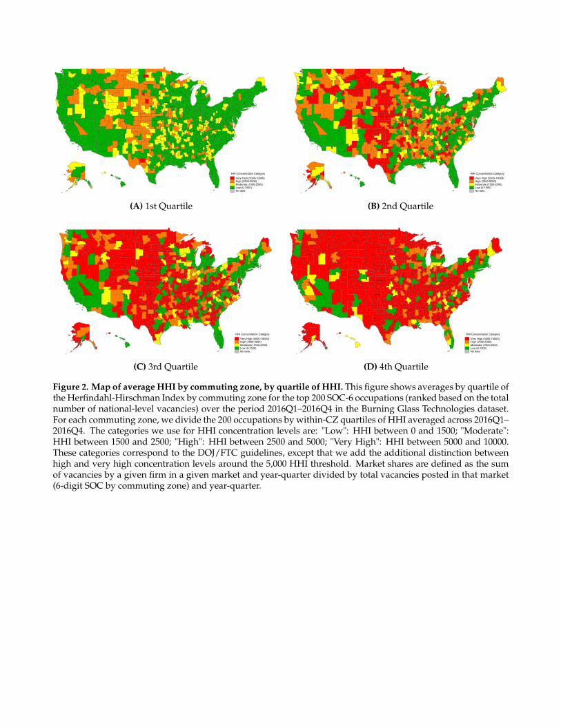
In Figure 2, we show the quartiles of HHI across the US, and reveal substantial heterogene-

ity in concentration across occupations even within a commuting zone. For each commuting

zone, we define quartiles of concentration of the top 200 6-digit SOC: the first quartile contains

the 25% least concentrated occupations on average over 2016 Q1-Q4 in that commuting zone,

the second quartile contains the next 25% least concentrated occupations in the commuting

zone, etc. Therefore, the quartiles can contain different occupations in each commuting zone

depending on the local level of the HHI. The map is color coded according to the average level

of the HHI in each quartile for each commuting zone. There are few commuting zones that

have highly concentrated occupations in the first quartile of concentration. Most of the com-

muting zones with highly concentrated occupations in the first quartile are in the middle of the

country at the west end of the Great Plains. At the other extreme, occupations in the fourth

quartile of concentration are extremely highly concentrated with an HHI above 5,000 in almost

all (86%) of the US commuting zones. Therefore, for much of the country, the least concentrated

25% of occupations have low concentration, while the most concentrated 25% of occupations

have extremely high concentration.

To further explore the variation in HHI by occupation, we report the average HHI in the

largest 30 occupations in Figure 4. There is substantial heterogeneity across the most frequent

occupations: over a third are highly concentrated, about one third are moderately concentrated

6Manning (2010) shows evidence on plant size that is consistent with lower monopsony power in cities.

12

and less than one third have low concentration. The most concentrated frequent occupation

is marketing managers and the least concentrated frequent occupation is registered nurses.

The top 5 most concentrated occupations are all high skilled occupations, while the rest of

occupations are more of a mix and of high and low skill.

The majority of labor markets are highly concentrated according to our baseline definition

of concentration. The frequency of highly concentrated labor markets is important for merger

policy because, as mentioned above, a merger challenger needs to identify only one market in

which anticompetitive results would be substantially likely to occur. At the same time, it is

also interesting to examine the extent to which US workers as a whole face high concentration.

When weighing each labor market by the number of employed workers, we find that HHI

is 1382 on average, implying an equivalent number of recruiting firms of 7.2. This relatively

low level of concentration is due to the fact that, as mentioned above, concentration is lower in

commuting zones with higher population. However, even after taking into account the unequal

distribution of employment across markets, we find that 17% of employment is in SOC-6 by

CZ by quarter cells that have high levels of concentration. Another 6% of employment is in

markets that are moderately concentrated. Overall, 23% of employment is in moderately or

highly concentrated markets, and these markets represent 65% of all labor markets.

The legal standard for merger review is that a merger that substantially reduces competition

in any market is illegal, and under the precedent of United States v. Philadelphia National

Bank, pro-competitive benefits in one market cannot be used to offset the loss of competition

in another. Therefore, the existence of many highly concentrated labor markets matters for

antitrust enforcement, even if most workers work in less concentrated markets.

So far, we have discussed variation in concentration while holding the market definition in

terms of 6-digit SOC by commuting zone by quarter fixed. We now examine how concentration

changes when we vary the definition of each one of these elements. Starting with occupation,

we report HHI for four alternative definitions. As mentioned above, there are reasons to think

that the job title may be the most appropriate definition of the labor market. When using

13

standardized job titles to define an occupational labor market, we find that the average con-

centration is higher than in the benchmark, at 5,323 (Table 1). This higher concentration was

to be expected, since job titles are more detailed than 6-digit SOC. When using job titles as the

definition of an occupation, 72% of markets are highly concentrated.

Next, instead of using the SOC-6 definition, we use the Burning Glass Technology (BGT)

occupation. This classification is based on the SOC, but expands or consolidates SOC categories

using the similarity of skills, education and knowledge requirements. This classification gives

results (Table 1) that are almost identical to the baseline. We then broaden the occupational

categories by using either the BGT broader occupation group or the 4-digit SOC. The BGT

broader occupation group categorizes occupations based on similar work functions, skills, and

profiles of education and training. When using either the BGT broader occupation group or the

4-digit SOC, HHI levels are very similar: the average market is roughly at the 2,500 threshold

for high concentration, and about one third of markets are highly concentrated.

We now examine the impact of alternative geographical market definitions. As would be

expected, county-level HHIs are higher than CZ-level HHIs, and state-level HHIs are lower

than CZ-level HHIs (Table 1). State-level HHIs are very low and only 4% of markets are highly

concentrated according to this definition. However, a state is very likely too broad a market.

By contrast, a county is smaller than a commuting zone and is sometimes used to define a

geographic market, e.g. by the Federal Reserve to calculate banking concentration (Federal

Reserve Bank of St. Louis, 2017). If we adopt the county as a definition of the geography for a

labor market, a whooping 74% of labor markets are highly concentrated.

Finally, we examine time aggregations other than the quarter. Table 1 shows that the average

HHI calculated using monthly data is higher than the baseline, and the HHI using semesters is

lower but still highly concentrated.

In summary, we find that reasonably defined local labor markets are highly concentrated

on average. In our preferred definition of the labor market, the majority of US labor markets

are highly concentrated (above 2,500 HHI).

14

5 Discussion

One potential explanation of firm-specific earnings premia (Card et al., 2016; Song et al.,

2016) is a lack of competition among employers: if job offers are not frequent enough to equi-

librate earnings of similar workers across firms, then firms likely have market power in wage

setting. The increase in the degree of inter-firm earnings inequality, especially since the dis-

persion of pure firm fixed effects has not increased (Song et al. (2016)), is an indication that

firm-level wage-setting power has become relatively more important. Empirical studies of the

declining frequency of incoming job offers for employed workers (Hyatt and Spletzer (2016)

and Molloy et al. (2016)) are also consistent with a decrease in labor market competition among

employers.

The estimates we offer of labor market concentration are comparable with estimates of mar-

ket concentration in many product markets that are considered concentrated in the Industrial

Organization literature, especially for those where geography is at least one element of market

definition. For example, Kwoka, Hearle and Alepin (2016) report an average HHI of 3930 in

their sample of high-traffic airline routes, and Steinbaum (forthcoming) calculates an average

airline route HHI around 5400 in recent years, using a less stringent criterion for route-level

traffic. Azar, Schmalz and Tecu (forthcoming) estimate mean route-level concentration at 5202.

Cooper et al. (2015) find that mean HHI in hospital markets, defined by number of beds

within a 15-mile radius, is 4160. For health insurers, for which the relevant market is the state,

given state-level insurance regulation, the same authors calculate mean HHI as 2120. Another

commonly-studied output market in which geography matters is retail groceries: Hosken, Ol-

son and Smith (2012) find that in markets in which a merger occurred during their study period

(2005-2009), the ex-ante HHI averaged 2334, while in their control group of markets that expe-

rienced no consolidation of any kind, concentration was 3368. Finally, concentration in local

banking markets is typically measured at the county level; Azar, Raina and Schmalz (2016)

estimate mean HHI for deposit-taking institutions is 1840. Altogether, many markets are very

15

concentrated. In this sense, what we find in labor markets is not anomalous.

However, a crucial final point to be made is that labor markets are different from the goods

markets which are the usual domain of antitrust analysis and hence of the concentration thresh-

olds contained in the Horizontal Merger Guidelines. Goods markets are typically thought of

as one-sided, and hence the extent of the market is delimited by the options among which con-

sumers substitute. Labor markets, on the other hand, are two-sided: workers not only have to

find an employer; they have to find an employer who is willing to hire them (Naidu, Posner

and Weyl, 2018). This implies that traditional concentration measures overestimate the options

available to workers, and thus underestimate concentration. Indeed, 55% of job offers are ac-

cepted by the non-employed, showing that in practice workers have few offers they could have

accepted (Faberman et al., 2017). The two-sided nature of labor markets therefore implies that

job choice sets are typically more restricted than product choice sets.

6 Conclusion

Since the release of Barkai (2016), Autor et al. (2017) and De Loecker and Eeckhout (2017),

and other papers documenting rising product market concentration and discussing its effect

on the labor market, there has been a great deal of academic and popular interest in whether

market concentration might be the cause of monopsony power, wage stagnation, and other

macro labor trends.

In this paper, we contribute to this growing debate by calculating measures of market con-

centration in local labor markets for the near-universe of 2016 online vacancy postings con-

structed by Burning Glass, and building on Azar, Marinescu and Steinbaum (2017). We have

shown that concentration is high (above 2,500 HHI) in 54% of US labor markets according to

our baseline market definition, and in at least a third of US labor markets according to alter-

native labor market definitions. Our results suggest that the anti-competitive effects of con-

centration on the labor market could be important. As detailed in Marinescu and Hovenkamp

16

(2018), the type of analysis we provide could be used to incorporate labor market concentration

concerns as a factor in the legal review of company mergers.

17

References

Artuc, Erhan, and John McLaren. 2015. “Trade policy and wage inequality: A structural anal-

ysis with occupational and sectoral mobility.” Journal of International Economics, 97: 28–41.

Artuc, Erhan, Shubham Chaudhuri, and John McLaren. 2010. “Trade Shocks and Labor Ad-

justment: A Structural Empirical Approach.” American Economic Review, 100: 1008–1045.

Ashenfelter, Orley, and Alan B. Krueger. 2017. “Theory and Evidence on Employer Collusion

in the Franchise Sector.” Princeton University Industrial Relations Section Working Paper.

DOI: 10.3386/w23396.

Ashenfelter, Orley C., Henry Farber, and Michael R. Ransom. 2010. “Labor market monop-

sony.” Journal of Labor Economics, 28(2): 203–210.

Autor, David, David Dorn, Lawrence F. Katz, Christina Patterson, and John Van Reenen.

2017. “The Fall of the Labor Share and the Rise of Superstar Firms.” National Bureau of

Economic Research Working Paper 23396. DOI: 10.3386/w23396.

Azar, Jose, Ioana Marinescu, and Marshall Steinbaum. 2017. “Labor Market Concentration.”

Azar, Jose, Martin Schmalz, and Isabel Tecu. forthcoming. “Anti-Competitive Effects of Com-

mon Ownership.” Journal of Finance.

Azar, Jose, Sahil Raina, and Martin Schmalz. 2016. “Ultimate Ownership and Bank Competi-

tion.”

Barkai, Simcha. 2016. “Declining Labor and Capital Shares.”

Baum-Snow, Nathaniel, and Ronni Pavan. 2012. “Understanding the City Size Wage Gap.”

The Review of Economic Studies, 79(1): 88–127.

18

Benmelech, Efraim, Nittai Bergman, and Hyunseob Kim. 2018. “Strong Employers and Weak

Employees: How Does Employer Concentration Affect Wages?”

BLS. 2017. “Unemployed persons by duration of unemployment.” Bureau of Labor Statistics.

Boal, William M., and Michael R Ransom. 1997. “Monopsony in the Labor Market.” Journal of

Economic Literature, 35(1): 86–112.

Bunting, Robert. 1962. Employer Concentration in Local Labor Markets. University of North Car-

olina Press.

Card, David, Ana Rute Cardoso, Joerg Heining, and Patrick Kline. 2016. “Firms and Labor

Market Inequality: Evidence and Some Theory.”

Carnevale, Anthony P, Tamara Jayasundera, and Dmitri Repnikov. 2014. “Understanding on-

line job ads data.”

CEA. 2016. “Labor market monopsony: trends, consequences, and policy responses.” White

House Council of Economics Adivsors.

Cooper, Zack, Stuart V. Craig, Martin Gaynor, and John Van Reenen. 2015. “The Price Ain’t

Right? Hospital Prices and Health Spending on the Privately Insured.”

De Loecker, Jan, and Jan Eeckhout. 2017. “The Rise of Market Power and the Macroeconomic

Implications.”

Deming, David, and Lisa B. Kahn. 2017. “Skill Requirements across Firms and Labor Mar-

kets: Evidence from Job Postings for Professionals.” National Bureau of Economic Research

Working Paper 23328. DOI: 10.3386/w23328.

Dix-Caneiro, Rafael. 2014. “Trade Liberalization and Labor Market Dynamics.” Econometrica,

82: 825–885.

19

Dube, Arindrajit, William T. Lester, and Michael Reich. 2016. “Minimum Wage Shocks, Em-

ployment Flows, and Labor Market Frictions.” Journal of Labor Economics, 34: 663–704.

Faberman, R. Jason, Andreas I. Mueller, Aysegül Sahin, and Giorgio Topa. 2017. “Job Search

Behavior among the Employed and Non-Employed.” National Bureau of Economic Research

Working Paper 23731. DOI: 10.3386/w23731.

Falch, Torberg. 2010. “The Elasticity of Labor Supply at the Establishment Level.” Journal of

Labor Economics, 28(2): 237–266.

Federal Reserve Bank of St. Louis. 2017. “Competitive Analysis and Structure Source Instru-

ment for Depository Institutions.”

Haltiwanger, John, Henry R. Hyatt, Lisa B. Kahn, and Erica McEntarfer. forthcoming. “Cycli-

cal Job Ladders by Firm Size and Firm Wage.” American Economic Journal: Macroeconomics.

Harris, Barry C., and Joseph J. Simons. 1991. “Focusing Market Definition: How Much Substi-

tution is Necessary The DOJ Merger Guidelines Part I: Market Definition 12 Research in Law

and Economics 207 (1989).” Journal of Reprints for Antitrust Law and Economics, 21: 151–172.

Hershbein, Brad, and Lisa B. Kahn. 2016. “Do Recessions Accelerate Routine-Biased Techno-

logical Change? Evidence from Vacancy Postings.” National Bureau of Economic Research

Working Paper 22762. DOI: 10.3386/w22762.

Hosken, Daniel, Luke M. Olson, and Loren Smith. 2012. “Do Retail Mergers Affect Competi-

tion? Evidence from Retail Grocery.”

Hyatt, Henry R., and James R. Spletzer. 2016. “The Shifting Job Tenure Distribution.” Labour

Economics, 41: 363–377.

Konczal, Mike, and Marshall Steinbaum. 2016. “Declining Entrepreneurship, Labor Mobility,

and Business Dynamism: A Demand-Side Approach.”

20

Kwoka, John, Kevin Hearle, and Philippe Alepin. 2016. “From the Fringe to the Fore-

front: Low Cost Carriers and Airline Price Determination.” Review of Industrial Organization,

48: 247–268.

Macaluso, Claudia. 2017. “Skill remoteness and post-layoff labor market outcomes.”

Manning, Alan. 2010. “The plant size-place effect: agglomeration and monopsony in labour

markets.” Journal of Economic Geography, 10(5): 717–744.

Manning, Alan. 2011. “Imperfect competition in the labor market.” Handbook of labor economics,

4: 973–1041.

Manning, Alan, and Barbara Petrongolo. 2017. “How Local Are Labor Markets? Evidence

from a Spatial Job Search Model.” American Economic Review, 107(10): 2877–2907.

Marinescu, Ioana, and Herbert Hovenkamp. 2018. “Anticompetitive Mergers in Labor Mar-

kets.” Social Science Research Network SSRN Scholarly Paper ID 3124483, Rochester, NY.

Marinescu, Ioana, and Roland Rathelot. 2017. “Mismatch Unemployment and the Geography

of Job Search.” American Economic Journal: Macroeconomics, forthcoming.

Marinescu, Ioana, and Ronald Wolthoff. 2016. “Opening the Black Box of the Matching Func-

tion: the Power of Words.” National Bureau of Economic Research Working Paper 22508.

DOI: 10.3386/w22508.

Matsudaira, Jordan D. 2013. “Monopsony in the Low-Wage Labor Market? Evidence from

Minimum Nurse Staffing Regulations.” The Review of Economics and Statistics, 96(1): 92–102.

Modestino, Alicia Sasser, Daniel Shoag, and Joshua Ballance. 2016. “Downskilling: Changes

in Employer Skill Requirements Over the Business Cycle.”

21

Molloy, Raven, Christopher L. Smith, Ricardo Trezzi, and Abigail Wozniak. 2016. “Under-

standing declining fluidity in the U.S. labor market.” Brookings Papers on Economic Activity,

183–237.

Naidu, Suresh, Eric N. Posner, and E. Glen Weyl. 2018. “Antitrust Remedies for Labor Market

Power.”

Ransom, Michael R, and David P. Sims. 2010. “Estimating the Firm’s Labor Supply Curve in

a “New Monopsony” Framework: Schoolteachers in Missouri.” Journal of Labor Economics,

28(2): 331–355.

Song, Jae, David J. Price, Fatih Guvenen, Nicholas Bloom, and Till von Wachter. 2016. “Firm-

ing Up Inequality.”

Staiger, Douglas O, Joanne Spetz, and Ciaran S Phibbs. 2010. “Is there monopsony in the

labor market? Evidence from a natural experiment.” Journal of Labor Economics, 28(2): 211–

236.

Starr, Evan, J. J. Prescott, and Norman Bishara. 2017. “Noncompetes in the U.S. Labor Force.”

Social Science Research Network SSRN Scholarly Paper ID 2625714, Rochester, NY.

Steinbaum, Marshall. forthcoming. “Airline Consolidation, Merger Retrospectives, and Oil

Price Pass-Through.”

Traiberman, Sharon. 2017. “Occupations and Import Competition: Evidence from Denmark.”

Yankow, Jeffrey J. 2006. “Why do cities pay more? An empirical examination of some compet-

ing theories of the urban wage premium.” Journal of Urban Economics, 60(2): 139–161.

22

Table 1. Summary statistics for labor market concentration, for the baseline and alternative market definitions.This table shows summary statistics for labor market Herfindahl-Hirschman Index (HHI) under various marketdefinitions, for the year 2016 using data from Burning Glass Technologies (BGT). The baseline is calculated usingcommuting zones for the geographic market definition, 6-digit SOC codes for the occupational market definition,aggregating the data at the quarterly level (and then averaging over quarters for a given CZ×SOC). In the alter-native definitions, the calculation is done by changing the baseline along one dimension (occupation, geography,time horizon). Except for the HHI weighted by employment, concentration is calculated over the top 200 SOC-6occupations (ranked based on the number of vacancies) over the period 2016Q1–2016Q4.

Mean Min Max 25th Pctile. 75th Pctile.Fraction

ModeratelyConcentrated

FractionHighly

Concentrated

Baseline market definition:

Number of Firms(Unweighted) 16.5 1.0 3069.8 1.5 10.0

HHI (Unweighted) 3953 3 10000 875 6667 0.11 0.54HHI (Weighted byBLS Employment) 1382 3 10000 101 1249 0.06 0.17

Alternative occupational definition:

HHI (By Job Title) 5323 3 10000 2232 8333 0.09 0.72HHI (By BGT Occupation) 3978 3 10000 875 6667 0.11 0.55HHI (By BGT Broader

Occupation Group) 2504 4 10000 363 3966 0.11 0.35

HHI (By 4-digit SOC) 2437 4 10000 339 3739 0.11 0.33

Alternative geographical definition:

HHI (By County) 5609 5 10000 2418 10000 0.08 0.74HHI (By State) 561 2 10000 79 422 0.02 0.04

Alternative time aggregation:

HHI (Monthly) 5767 10 10000 2822 8651 0.07 0.77HHI (Semesterly) 2850 2 10000 426 4300 0.12 0.37

Very High (5000-10000)High (2500-5000)Moderate (1500-2500)Low (0-1500)No data

HHI Concentration Category

Figure 1. Average HHI by commuting zone, based on vacancy shares. This figure shows the average of theHerfindahl-Hirschman Index by commuting zone code for the top 200 SOC-6 occupations (ranked based on thenumber of vacancies) over the period 2016Q1–2016Q4 in the Burning Glass Technologies dataset. The categorieswe use for HHI concentration levels are: "Low": HHI between 0 and 1500; "Moderate": HHI between 1500 and2500; "High": HHI between 2500 and 5000; "Very High": HHI between 5000 and 10000. These categories cor-respond to the DOJ/FTC guidelines, except that we add the additional distinction between high and very highconcentration levels around the 5,000 HHI threshold. Market shares are defined as the sum of vacancies by a givenfirm in a given market (6-digit SOC by commuting zone) and year-quarter divided by total vacancies posted inthat market and year-quarter.

Very High (5000-10000)High (2500-5000)Moderate (1500-2500)Low (0-1500)No data

HHI Concentration Category

(A) 1st Quartile

Very High (5000-10000)High (2500-5000)Moderate (1500-2500)Low (0-1500)No data

HHI Concentration Category

(B) 2nd Quartile

Very High (5000-10000)High (2500-5000)Moderate (1500-2500)Low (0-1500)No data

HHI Concentration Category

(C) 3rd Quartile

Very High (5000-10000)High (2500-5000)Moderate (1500-2500)Low (0-1500)No data

HHI Concentration Category

(D) 4th Quartile

Figure 2. Map of average HHI by commuting zone, by quartile of HHI. This figure shows averages by quartile ofthe Herfindahl-Hirschman Index by commuting zone for the top 200 SOC-6 occupations (ranked based on the totalnumber of national-level vacancies) over the period 2016Q1–2016Q4 in the Burning Glass Technologies dataset.For each commuting zone, we divide the 200 occupations by within-CZ quartiles of HHI averaged across 2016Q1–2016Q4. The categories we use for HHI concentration levels are: "Low": HHI between 0 and 1500; "Moderate":HHI between 1500 and 2500; "High": HHI between 2500 and 5000; "Very High": HHI between 5000 and 10000.These categories correspond to the DOJ/FTC guidelines, except that we add the additional distinction betweenhigh and very high concentration levels around the 5,000 HHI threshold. Market shares are defined as the sumof vacancies by a given firm in a given market and year-quarter divided by total vacancies posted in that market(6-digit SOC by commuting zone) and year-quarter.

020

0040

0060

0080

00H

HI

8 10 12 14 16Log(CZ Population)

Figure 3. Binned scatter of HHI and Population. This figure shows a binned scatter of the Herfindahl-HirschmanIndex by commuting zone for the top 200 SOC-6 occupations (ranked based on the number of vacancies) over theperiod 2016Q1–2016Q4 in the Burning Glass Technologies dataset, and log of population in the correspondingcommuting zone in 2016 (based on Census data).

0 1,000 2,000 3,000 4,000Average HHI

Registered Nurses

Heavy and Tractor-Trailer Truck Drivers

Customer Service Representatives

Sales Representatives, Wholesale and Manufacturing, Except Technical and Scientific Products

First-Line Supervisors of Retail Sales Workers

Retail Salespersons

Maintenance and Repair Workers, General

Licensed Practical and Licensed Vocational Nurses

Nursing Assistants

Laborers and Freight, Stock, and Material Movers, Hand

Medical and Health Services Managers

Managers, All Other

Secretaries and Administrative Assistants, Except Legal, Medical, and Executive

Combined Food Preparation and Serving Workers, Including Fast Food

Stock Clerks and Order Fillers

First-Line Supervisors of Food Preparation and Serving Workers

Human Resources Specialists

Computer Occupations, All Other

Sales Managers

General and Operations Managers

Accountants and Auditors

Financial Managers

Bookkeeping, Accounting, and Auditing Clerks

Software Developers, Applications

Computer User Support Specialists

Computer Systems Analysts

Management Analysts

Database Administrators

Financial Analysts

Web Developers

Marketing Managers

Figure 4. Average HHI by occupation, based on vacancy shares, for the largest 30 occupations. This figure showsthe average of the Herfindahl-Hirschman Index by 6-digit SOC occupation code for the 30 largest occupations asmeasured by number of vacancies over the period 2016Q1–2016Q4 in the Burning Glass Technologies dataset.Market shares are defined as the sum of vacancies posted by a given firm in a given market (6-digit SOC bycommuting zone) and year-quarter divided by total vacancies posted in the website in that market and year-quarter.