Diatom-based stream bioassessment: the effects of rare taxa and

live/dead ratio

Dissertation Proposal

Ph. D. in Environmental Sciences and Resources

Submitted by: Nadezhda D. Gillett

January 2009

Defense Date: 12:00 pm, February 3, 2009

Dissertation Committee

Portland State University

Committee Members:

Dr. Yangdong Pan, Chair

Dr. Joseph Maser

Dr. Ian Waite

Dr. J. Alan Yeakley

Graduate Office Representative: Dr. Jiunn-Der Duh

2

General Introduction

The assessment of ecological integrity in streams and rivers is essential for the

healthy, social and economic well-being of humans. However, human-induced stressors

(e. g. agriculture, logging, urbanization, sewage contamination, etc.) alter the stream

environment and the aquatic organisms by changing their habitat structure, flow regime,

water quality, energy source and biotic interactions (Karr and Chu, 1999). Conceptually

such alterations may cause the biota to respond in a predictable way by changing its

energetics, nutrient cycling and community structure (Odum, 1985). Bioassessment

focuses on changes in biotic community structure and function in response to human

disturbance.

Diatom-based assessment has been an integral part of both national and regional

bioassessment programs (Stevenson and Bahls, 1999; Peck et al., 2006). Accuracy and

precision in diatom-based bioassessment need to be improved to meet the increasing

demands of water resource management. Diatoms, a group of algae, are good

bioindicators of water quality in streams and rivers (Stevenson and Pan, 1999). As

primary producers, they are at the base of the food web in streams. Diatoms, with short

life cycles, respond quickly to a variety of environmental conditions such as organic

pollution (Lange-Bertalot, 1979), siltation (Bahls, 1993), pH (Pan et al., 1996) and

eutrophication (Kelly and Whitton, 1995; Potapova and Charles, 2007). Diatom

assemblages are species rich and each species may provide information about their

environment (Lowe and Pan, 1996). Conventional diatom-based bioassessment

programs, however, often draw assessment conclusions based on the responses of the

common taxa to the environment, while the rare taxa in the diatom assemblages, regarded

as noise, are often excluded from final assessment analyses or down-weighted (Pan et al.

1996, 2000; Potapova and Charles, 2002, 2003). Based on the niche theory, several

researchers assume that rare species may have narrow environmental requirements and

therefore may be used as good indicators of pollution (Gaston, 1994; Potapova and

Charles, 2004). This notion is not well supported by the current diatom literature.

Bioassessment uses living organisms to evaluate environmental quality, with

diatoms being an exception. A diatom sample comprises a mixture of live (chloroplast

3

containing siliceous cell walls) and dead (only siliceous cell walls) individuals which are

not distinguished from each other in the conventional diatom analysis (Charles et al.,

2002). This analysis involves the use of strong acid to remove the organic material in

diatom cells to reveal the fine morphological features of their cell walls, which allows

diatom identification to the lowest possible taxonomic level. It is unclear whether

differentiating live and dead diatoms in an assemblage would significantly improve the

accuracy and precision of diatom-based bioassessment. Several researchers have

suggested that assemblages generated by the traditional method may better integrate

spatial and temporal variability of environmental conditions in the sampled stream and its

watershed, because the accumulation of live and dead diatoms over time may provide

broad environmental information (Cox, 1998; Stevenson and Pan, 1999). However,

Pryfogle and Lowe (1979) concluded that the traditional counting technique might mask

the specific response of the live resident taxa to the local environmental conditions. In

addition, dead diatoms from adjacent habitats might be a significant source of error in

characterizing diatom communities and their signals about the local environment (Round,

1998).

The US Environmental Protection Agency’s Western Environmental Monitoring

and Assessment Program (WEMAP) provides a great opportunity to enhance the quality

of diatom-based assessment. WEMAP sampled the western US streams and rivers with

the major objective to assess the status of surface waters in the west. The project

collected an extensive set of physical, chemical and biological data over the course of

five years in 12 western states. Another important task of this project is to develop and

evaluate the tools for assessing ecological conditions. Both of these objectives, as well as

its large spatial coverage and probability-based sampling design, allow inferences to be

made from a small number of samples about the extent of the whole study area. The

extensive study area provides potential good natural and disturbance gradients which can

be used to explore the roles of live/or dead diatoms and rare diatom taxa in

bioassessment.

My proposed research focuses on the potential roles of both rare taxa and

live/dead diatoms in diatom-based stream bioassessment (Fig. 1). Specifically, I want to

evaluate whether rare diatom taxa with either low abundance or small range size have

4

narrower ecological niches than common taxa and if so, I want to assess if the number of

rare taxa can be used as an indicator of environmental conditions. I also want to assess

the relationships between live/dead diatoms and human disturbance from a large scale

study (12 western states) and a small scale study (Oregon coastal region).

Fig. 1. Flow diagram of proposed research plan.

Background Information

Bioassessment

The main goal of bioassessment is to evaluate whether a site or a system of

interest (test site) is impaired based on biological indicators. This is usually done by a

comparison to reference conditions with high physical, chemical and biological quality.

The reference conditions can be defined for a region or for a site depending on the

assessment objectives (US EPA, 2002). The regional reference condition represents

natural state within a region for ecosystems with different geographical features (e.g.,

climate, soil, topography and vegetation) and their biological communities (Hughes et al.,

1986). The site-specific approach evaluates the conditions upstream from a point source

pollution or in a matching watershed (Hughes et al., 1986). Due to the pervasive nature of

human disturbance, a reference condition free of human disturbance may not exist and

Importance of rare taxa in diatom-based stream bioassessment

Do rare taxa with small range size inhabit narrow ecological niches?

Live diatoms in bioassessment: a small regional study

Do different metrics of diatom rarity respond to natural conditions or to human disturbance?

Are the diatom assemblages generated by counting the traditional acid cleaned samples different from the live diatoms in the undigested samples?

Do the assemblages from the two counts differ in their responses to the measured environmental variables?

Live diatoms in bioassessment: a large scale study

Can percent live diatoms be used as a metric of human disturbance?

Dead diatoms in bioassessment

Can percent dead diatoms be used as a metric of human disturbance?

Do rare taxa with low abundance inhabit narrow ecological niches?

5

the phrase “reference condition for biological integrity” (biological condition without

human disturbance in a watershed, e.g., national parks) has been proposed (Stoddard et

al., 2006). Several definitions for reference conditions include: minimally disturbed

condition (absence of significant human disturbance), least disturbed condition (least

impacted current condition), historical condition (known lack of human influence in the

past) or best attainable condition (desirable future condition with better management)

(Stoddard et al., 2006). Reference site selection is often determined by proximity and

influence by human population density and distribution, road density and land use in the

watershed (logging, mining, agriculture, grazing and urbanization). Biological indicators,

organisms with well-known response to disturbance, are used to detect deviations from

reference conditions (Davies and Jackson, 2006).

Bioassessment uses different groups of organisms (e.g., algae, macroinvertebrates

and fish) to evaluate the environmental conditions of waters. Biological assemblages are

often characterized using different biological attributes such as diversity, abundance, and

functional groups. Diversity measures play an important role in bioassessment, because

diversity is perceived as a correlate of environmental well being (Magurran, 2004).

Diversity can decrease with disturbance, increase or have mixed response depending on

the type of pollution (Patrick et al., 1954; Patrick, 1967; Stevenson, 1984, 2006). Under

stressed conditions, species richness decreases while dominance increases (increase in

unevenness of species abundances) (Patrick, 1973; Odum, 1985). Many statistical models

assume that the abundance of an organism is related to its ecological importance

(Magurran, 2004). Functional groups are based on trophic level (e. g., herbivores,

omnivores, carnivores, predators) (Karr, 1981), feeding habits (e. g., filterers, collectors,

gatherers) (Vannote et al., 1980) or other processes that different community members

perform.

Rare taxa in bioassessment

The importance of rare species in bioassessment programs is a topic of big

debates. Rare taxa often occur with low abundances or in a limited number of sites.

Most sampling methods are not designed to collect rare species adequately, which

subsequently affects their identification and enumeration, and results interpretation.

6

Consequently, their ecology is not well studied. The supporters of using rare species in

bioasessment state that because we do not know enough about them, exclusing rare taxa

in bioassessment may lose valuable information about their environment (Karr, 1991,

1999; Fore et al., 1996; Cao et al., 1998, 2001; Cao and Williams, 1999; Nijboer and

Schmidt-Kloiber, 2004). These researchers assume that rare taxa may inhabit narrow

ecological niches and therefore may be good indicators of very specific conditions

(Magurran, 2004). In contrast, other researchers argue that rare taxa should be excluded

because they may simply add noise to data analyses (Marchant, 1999, 2002; Hawkins et

al., 2000; Van Sickle et al., 2007). Some predictive models exclude rare

macroinvertebrate taxa from the model development (Marchant et al., 1997; Reynoldson

et al. 1995; Carlisle et al. 2008), while others do not (Wright et al., 2000). Another

argument against using rare taxa in bioassessment is that the information contained in

them is already provided by common species which are better quantified (Marchant,

1999, 2002). Most studies that looked at the effects of rare species exclusion on the

detection of major environmental gradients found that common species recovered these

gradients well (Cao et al., 1998; Van Sickle et al., 2007; Hawkins et al., 2000; Nijboer

and Schmidt-Kloiber, 2004; Lavoie et al., 2009).The few studies that analyzed rare

species exclusively recommended against their exclusion from the analysis (Faith and

Norris, 1989; Nijboer and Schmidt-Kloiber, 2004). Faith and Norris (1989) compared

the responses of common and rare macroinvertebrate species to their environment and

found that the rare species correlated with more environmental variables than the

common taxa. This finding made them suggest that the distribution and abundance of rare

taxa might be determined by a different set of environmental variables than common

taxa. Nijboer and Schmidt-Kloiber (2004) found that when rare taxa with low relative

abundances were excluded from the analysis, the sites were classified in higher

ecological quality class, but when rare taxa with narrow distribution ranges were

excluded the results were the opposite.

Live/dead diatoms in stream bioassessment

The development of benthic diatom communities in lotic systems is similar to the

development of terrestrial plant communities. They start as two-dimensional communities

7

consisting of small adnate or prostrate individuals and develop with time into three-

dimensional diatom mats of erect, stalked and chain-forming species (Patrick, 1976;

Hoagland et al., 1982; Korte and Blinn, 1983). These mats, commonly referred as

‘periphyton’, comprise of not only diatoms, but of fungi, bacteria, organic debris and

other algal groups such as green algae. Since diatoms are its major component, the two

terms are used interchangeably in this study (Fig. 2). As the early colonizers are replaced

by later successional species which overshadow them and deplete them from nutrients,

the pioneer species perish and are either washed away by the current or trapped within

the diatom matrix. As a result, mature periphyton mats might have high numbers of live

diatoms or high numbers of dead diatoms (Peterson et al., 1990). Biological assessment

of water quality uses living organisms as indicators of environmental conditions, but in

diatom analysis live and dead diatoms are not distinguished from each other. This is a

result of the diatom sample processing which requires removal of all organic material to

aid in their identification based on the morphological features of their cell walls. This

technique may result in overestimated cell density and species diversity (Pryfogle and

Lowe, 1979; Potapova and Charles, 2005). For example, higher diversity is generally

associated with reference conditions (Magurran, 2003; Odum, 1985), and a site with

overestimated diversity might be classified as being in better ecological condition than it

actually is.

Fig. 2. Periphyton community succession (from Hoagland et al., 1982).

8

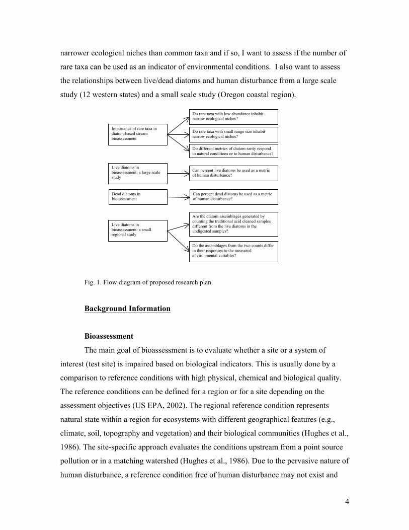
The accumulation of live/dead diatoms is a function of reproduction rate, death

rate, immigration and emigration rates (McCormick and Stevenson, 1991; Stevenson and

Peterson, 1991), age of the community (Peterson et al., 1990; Steinman and McIntire,

1990), disturbance (Peterson and Stevenson, 1992; Peterson, 1996), predation (Peterson,

1987; Steinman et al., 1987), and resource supply (Steinman and McIntire, 1986;

Peterson and Stevenson, 1989; Stevenson et al., 1991). In flowing waters periphyton is

frequently removed from the substrata by current, spates, substratum instability and

grazing activity (Fig. 3) (Korte and Blinn, 1983). These dislodged clumps of periphyton

become suspended in the water column (drift) and provide continuous supply of potential

colonists of newly cleared substrata downstream (Peterson, 1996). Thus, emigration and

immigration are important processes which affect benthic diatom species composition

(Stevenson and Peterson, 1991). Emigration is positively influenced by disturbance from

grazing and stream discharge while immigration is negatively affected by them. Early-

successional species utilize different growth strategies which include high immigration

coefficients and high drift abundances while late-successional species have high

reproduction rates (McCormick and Stevenson, 1991). Death rate may become important

at later stages of succession when the accumulated biomass of upper layers prevents the

underlying ones from vital resources. With time and in the absence of disturbance, the

periphyton mat grows thicker, but it also becomes more susceptible to sloughing

(Hoagland et al. 1982; Peterson et al., 1990). The thickness of the periphyton mat is

controlled by disturbance and predation. When either one is high, the benthic community

is dominated by prostrate tightly attached to the substrate diatoms. When either one is

low, the periphyton mat has a complex three-dimensional structure. Live/dead diatom

accumulation is also influenced by the resources required for its development (e. g.,

space, nutrients and light) (Patrick, 1967, Steinman and McIntire, 1986; Stevenson et al.,

1991). The amount of live diatoms might be higher in erosional habitats compared to

depositional ones. The former usually provide dissolved nutrients with the fast flowing

water, while the latter serve as sinks for dislodged live and dead individuals. Ultimately,

large-scale factors (climate, geology and land use) determine the resources, while biotic

factors and abiotic stressors affect the structure and function of benthic algal assemblages

in streams (Stevenson, 1997).

9

Fig. 3. Live/dead diatom accumulation and loss (modified after Biggs, 1996).

Western Environmental Monitoring and Assessment Program (WEMAP)

Sampling design and site selection

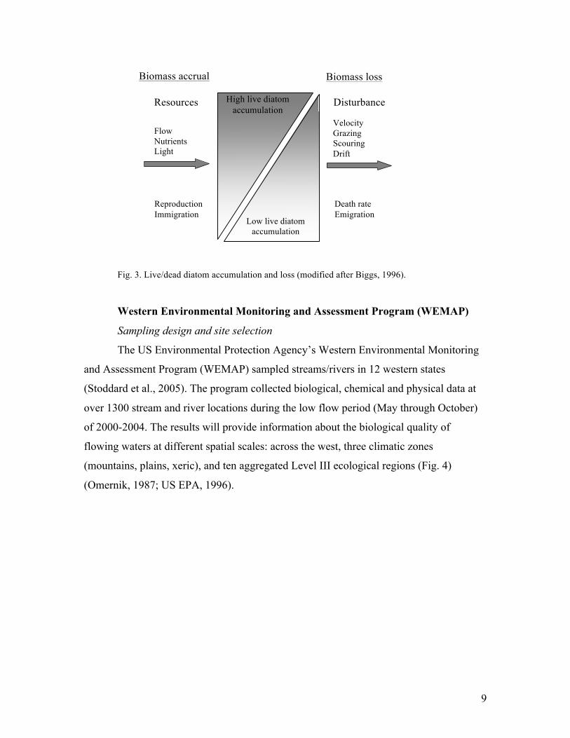
The US Environmental Protection Agency’s Western Environmental Monitoring

and Assessment Program (WEMAP) sampled streams/rivers in 12 western states

(Stoddard et al., 2005). The program collected biological, chemical and physical data at

over 1300 stream and river locations during the low flow period (May through October)

of 2000-2004. The results will provide information about the biological quality of

flowing waters at different spatial scales: across the west, three climatic zones

(mountains, plains, xeric), and ten aggregated Level III ecological regions (Fig. 4)

(Omernik, 1987; US EPA, 1996).

Disturbance Resources

Reproduction Immigration

Flow Nutrients Light

Death rate Emigration

Velocity Grazing Scouring Drift

Low live diatom accumulation

Biomass accrual

High live diatom accumulation

Biomass loss

10

Fig. 4. WEMAP study area with sampling locations within three spatial scales: West-wide, three

climatic zones (mountains, plains, xeric) and ten aggregated Level III ecoregions (Omernik, 1987).

A key element of the WEMAP is its probability-based sampling design for site

selection. This feature allows for the results from a small number of samples to be

applied to the whole area of interest with a known level of uncertainty. Sampling sites are

selected from digital 1:100,000-scale USGS hydrographic maps of perennial and non-

perennial streams and rivers following spatially-balanced stratified random sampling

design (Herlihy et al., 2000; Hughes et al., 2000; Stevens  and  Olsen,  2004). A randomly

placed grid of triangular points and their hexagonal tessellations are overlaid with the

map of the continental US, allowing for a finer or coarser grid depending on the desired

sample size and spatial coverage (Herlihy et al., 2000). Sampling sites are identified after

a two-stage selection process. In the first stage, 40 km2 hexagons are delimited and the

length of streams within each one of them is calculated (Fig. 5). In the second stage,

individual sampling sites are selected from a subset of the first-stage sample after

examination of maps, aerial and satellite imagery, and other types of data (Herlihy et al.,

2000). All stream segments from the first-stage process (within a hexagon) are randomly

arranged in a straight line and sampling points are randomly selected at equal intervals

after a random start. The length of the intervals is determined by the length of the line

divided by the number of desired samples. The total sampled stream length was 304,544

11

km or 48% of the original frame length, and 72% of the target stream length (Stoddard et

al., 2005).

Fig. 5. An example of EMAP site selection process in the Mid-Atlantic. A map of stream network

overlaid with 40 km2 hexagons (from Herlihy et al., 2000). See text for explanation.

Field sampling

Streams  were  sampled  with  wadeable-­‐stream  protocols  (Peck  et  al.  2006),  whereas  

rivers  were  sampled  with  rafts  and  boatable-­‐river  protocols  (Peck  et  al.,  in  

press).WEMAP employs standardized reach length which increases in proportion to

stream size. Each sampling site (X-site on Fig. 6) is positioned in the center of the

sampling reach whose length is 40x the average stream wetted width or a minimum of

150 m (Kaufmann et al., 1999). Eleven equally spaced transects (A-K, Fig. 6) are

delineated along the sampling reach.

Stream flow

B

E C

D F

G H I

A

R

L

C

R

L

C R

L

C

J

R

K

L

X-site

Total reach length = 40 times mean wetted width at X-site (min = 150 m)

12

Fig. 6. WEMAP sampling reach features. The sampling site (X-site) lays in the center of the sapling reach which is defined by 11 equally spaced transects (A-K). Biological data are collected on the left (L), center (C) or the right (R) side of the stream, after a random start. Transects delineate stream reach which equals the length of 40 times the mean wetted width at the X-site. See text for details.

A grab sample from the middle of the stream is collected for water chemistry

analysis. It is used to determine acid-base status, trophic condition (nutrient enrichment),

chemical stressors and classification of water chemistry type (Herlihy, 2006). Water

chemistry measurements include major cations (Ca2+, Mg2+, Na+, K+) and anions (Cl–,

NO3–, SO4

2–), nutrients (total nitrogen, total phosphorus, NO3–/NO2

–-N, NH3), turbidity,

color, pH, conductivity, dissolved oxygen, dissolved organic and inorganic carbon. They

are analyzed following standard methods (US EPA, 1989). Physical habitat

characteristics are summarized (mean, standard deviation) from 20-100 measurements

per site (Kaufmann et al., 1999). Physical habitat is measured along the sampling reach to

determine channel dimensions and gradient, substrate size and type, habitat complexity

and cover, riparian vegetation cover and structure, anthropogenic alterations and channel-

riparian interaction (Kaufmann, 2006). The landscape component of WEMAP includes

soils, topography, climate, vegetation and land use. Watershed boundaries are delineated

from 1:24,000-scale USGS topographic maps and USGS’s 30-m digital elevation models

(DEMs). They are used to calculate watershed area, slope and elevation. Watershed land

use/cover were characterized from the USGS 1992 National Land Cover Dataset.

One periphyton sample is collected at ¼, ½ or ¾ of the distance to the stream

bank for each of the 11 transects. A surface area of 12-cm2 is scraped with a toothbrush

from rock/wood substrates (erosional habitat) or soft sediments are vacuumed with a 60-

mL syringe (depositional habitat). All 11 samples per reach are combined into one

composite sample which is preserved with 37% formalin.

Chapter I. The importance of rare taxa in diatom-based stream

bioassessment.

Rarity is a relative term and it depends on the sampling protocol and scale, time of

the year, sample size and survey intensity (Cao et al., 2001). There is no universal

definition of rarity, but the most popular classification includes geographic range (large

13

or small), local population size (large or small) and habitat specificity (wide or narrow)

(Rabinowitz, 1981). The combinations between them (except for large range, large

population and wide habitat specificity) represent seven forms of rarity. Most commonly

rarity is defined in terms of low abundance and/or small range size (Gaston, 1994). Some

researchers define rarity as: taxa with less than 1% relative abundance in a sample or in

less than 10 sites from the dataset (Potapova and Charles, 2004), taxa with at least 2%

relative abundance in 1 to 10 sites (Potapova and Charles, 2002), taxa with less than 5

individuals in a sample (Nijboer and Schmidt-Kloiber, 2004), taxa which occur at less

than 5% of the sites (Carlisle et al., 2008) and taxa with less than 50% probability of

being captured (Hawkins et al., 2000). Gaston (1994) suggested a “quartile” definition of

rarity: all taxa whose abundance or distribution falls within the first quartile (25th

percentile) are considered rare.

Causes of rarity may include breeding system biased away from sexual

reproduction, poor dispersal ability, low level of genetic polymorphism, low competitive

ability, narrow resource usage, high trophic level, and larger body size (for taxa with low

abundance) or smaller body size (for taxa with small geographic ranges) (Gaston, 1994).

Not all of these causes of rarity are necessarily applicable to diatoms (e. g., high trophic

level or breeding system) (Fig. 7). Diatom rarity may be associated with poor dispersal

and competitive ability, narrow resource usage and low genetic polymorphism. The

proposed narrow resource usage leads to the assumption that rare taxa are sensitive to

environmental conditions (Gaston, 1994; Stevenson and Pan, 1999; Potapova and

Charles, 2004). This conclusion is based on the niche concept which describes the

environmental requirements of species (Grinell, 1917). The niche width (breadth) is the

range of environmental conditions in which a species is observed to survive and

reproduce (Gaston, 1994). According to Gause’s axiom (1934), no two species can

coexist in a single niche. Therefore, narrow niche width will distinguish a species as a

good bioindicator. However, there is little evidence that rare taxa have narrower

ecological niches than common ones (Gaston, 1994). Gaston (1994) suggested that rare

species were common in the past when there was no human disturbance, but because they

are sensitive to it, their abundances and ranges are reduced now. Recently, some

researchers assessed the potential bioassessment value of rare diatoms in streams

14

(Potapova and Charles, 2004; Lavoie et al., 2009). However, their results were not

conclusive.

Fig. 7. Generic model for causes of rarity and their outcomes for species (modified after Gaston, 1994). The names in italic do not apply to diatoms.

The roles of rare species in bioassessment are not clear. Hawkins et al., (2000)

concluded that rare macroinvertebrates were increasing in abundance at impacted sites

compared to reference sites, while Potapova and Charles (2004) found that the number

and abundance of rare diatoms was decreasing not only along a human disturbance

gradient, but also with elevation. However, Potapova and Charles (2004) used a very

narrow definition of rarity (species that occur with 2% relative abundance in 1 to 10 sites)

and correlation analysis to evaluate its relationship with a gradient of human disturbance.

Faith and Norris (1989) compared the responses of common and rare macroinvertebrate

species to their environment and found that the rare species correlated with more

environmental variables than the common taxa. However, it was unclear whether their

findings were due to the much bigger number of rare taxa or not. Nijboer and Schmidt-

Kloiber (2004) found that when macroinvertebrate taxa with low relative abundances

were excluded from the analysis, the sites were classified as having high ecological

Good Poor

Sexual High

Poor Narrow High

Good Broad Low

Asexual Low

Competitive ability Resource usage Trophic level

Dispersal ability

Breeding system Genetic polymorphism

Rare species

Common species

15

quality, but when taxa with narrow distribution ranges were excluded the results were the

opposite. They suggested that taxa with low relative abundances were associated with

human disturbance, while taxa with narrow distribution ranges were indicators of

reference conditions in the Netherlands. The recommendation of the authors was to

avoid excluding rare taxa, either with low abundance or small distribution range, from

ecological assessments and to develop a metric which includes the number of taxa with

small distribution ranges (Nijboer and Schmidt- Kloiber, 2004).

Proposed Research Plan:

Objectives. - I want to evaluate whether rare diatom taxa have narrower

ecological niches than common taxa and if so, I want to assess if the number of rare taxa

can be used as good indicators of environmental condition.

Methods

Dataset. - The site selection and field sampling were conducted as part of the

WEMAP protocols outlined above. Water chemistry, physical habitat, landscape

characteristics and diatom data were collected from perennial streams and rivers in 12

western states. A subset of 1037 streams and rivers with 600 diatom counts were used for

this analysis.

Diatom analysis. - A small amount of each composite diatom sample was acid-

digested and used for the preparation of one permanent microscope slide (Patrick and

Reimer, 1966). A minimum of 600 diatom valves were counted and identified to the

lowest possible taxonomic level (mainly species) at 1000x under a light microscope. The

diatom taxonomy followed primarily Krammer and Lange-Bertalot (1986, 1988, 1991a,

b) and Patrick and Reimer (1966, 1975).

Data analysis. - To evaluate the width of ecological niche of rare taxa, I will use

the weighted averaging approach (ter Braak and Looman, 1986). This method is founded

on the idea that a single environmental variable determines the species composition at a

site and that each species has bell-shaped response curve with regard to this variable. The

theoretical base for the weighted averaging approach is the species packing model

(MacArthur and Levins, 1967), which utilizes the idea that species occupy maximally

separated niches with respect to a limiting resource. Therefore, their response curves

should have minimal overlap and equally spaced indicator values. The species response

16

curve can be summarized as species optimum (indicator value, mode of the curve) and

tolerance (ecological amplitude). Species optimum is calculated by averaging the

environmental variable over the samples where the species is present weighted by the

species abundance in the sites. Tolerance is calculated as the weighted standard deviation

of species abundance in the sites. To uncover the most important environmental variables

in the data, I will run principal component analysis (PCA). PCA reduces the

dimensionality of complex multivariate data to detect structure in the relationships

between variables. The first principal axis captures most of the variation in the data and

the variable with highest loading on this axis is the one most strongly associated with it.

This variable will be used to calculate the weighted averages for the species. If several

variables load heavily on the first principal axis, I will select the most meaningful ones in

terms of diatom ecology. The weighed averaging results for the species (common, rare

with low abundance and rare with small range) will be summarized in a table where they

will be represented by the species optima and tolerance. If the tolerances of rare taxa

cover narrower part of the gradients of the most important variables compared to

common taxa, this will suggest that rare taxa may have narrower environmental niches.

Diatom counts will be represented as percentage of total species counts per site

(relative abundance). The following diatom rarity metrics, expressed as number of taxa,

will be employed: taxa with < 1% relative abundance in a sample and taxa with < 1%

relative abundance in the dataset or in a region (ecoregion, watershed or hydrologic unit).

I will also calculate frequency of occurrence and regional presence. In addition, Gaston’s

“quartile” definition of rarity will also be explored as potential indicator in diatom

bioassessment (Table 1).

Table. 1. Rarity metrics and their definitions.

Rarity metric Definition

Sample rare 1% taxon with relative abundance < 1% in a sample Region rare 1% taxon with relative abundance < 1% in the dataset or a region Regional presence number of sites where a taxon occurs within an ecoregion, a

watershed or a hydrologic unit Frequency of occurrence number of sites where a taxon occurs "Quartile" rare taxa with abundance or frequency of occurrence within the

1st quartile (25th percentile)

17

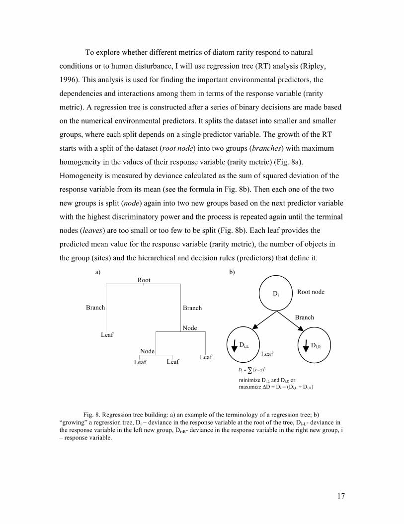
To explore whether different metrics of diatom rarity respond to natural

conditions or to human disturbance, I will use regression tree (RT) analysis (Ripley,

1996). This analysis is used for finding the important environmental predictors, the

dependencies and interactions among them in terms of the response variable (rarity

metric). A regression tree is constructed after a series of binary decisions are made based

on the numerical environmental predictors. It splits the dataset into smaller and smaller

groups, where each split depends on a single predictor variable. The growth of the RT

starts with a split of the dataset (root node) into two groups (branches) with maximum

homogeneity in the values of their response variable (rarity metric) (Fig. 8a).

Homogeneity is measured by deviance calculated as the sum of squared deviation of the

response variable from its mean (see the formula in Fig. 8b). Then each one of the two

new groups is split (node) again into two new groups based on the next predictor variable

with the highest discriminatory power and the process is repeated again until the terminal

nodes (leaves) are too small or too few to be split (Fig. 8b). Each leaf provides the

predicted mean value for the response variable (rarity metric), the number of objects in

the group (sites) and the hierarchical and decision rules (predictors) that define it.

Fig. 8. Regression tree building: a) an example of the terminology of a regression tree; b)

“growing” a regression tree, Di – deviance in the response variable at the root of the tree, Di,L- deviance in the response variable in the left new group, Di,R- deviance in the response variable in the right new group, i – response variable.

|Root

Branch

Node

Branch

Node Leaf

Leaf Leaf

Leaf

a)

Di

Di,L

Root node

Branch

Leaf

Di,R

b)

minimize Di,L and Di,R or maximize ∆D = Di – (Di,L + Di,R)

2)( xxDi ∑ −=

18

The resulting full tree may explain the variability in the response variable well but

may have limited predictive power. Therefore, cross-validation is used to trim the tree

and produce a less complex final tree. Cross-validation is done by splitting the original

dataset in two subsets and using 90% of it for model building (calibration dataset) and

10% for testing (validation dataset). This results in many tree models with different sizes

(number of splits). The difference between the observed and predicted values of the

response variable in the validation dataset is used to calculate the model prediction error

for each tree size (Fig. 9a). This cross-validation process is repeated again with another

90% of the data as calibration dataset and 10% as validation dataset and generates

another set of prediction errors for the different tree sizes. The prediction errors from

each cross-validation run are used to calculate the relative prediction error for the

different tree sizes. The size of the final tree model is decided by plotting the relative

prediction errors against the number of splits (tree sizes) (Fig. 9b). The final tree is

selected by the 1-SE rule (i. e., the tree within one standard error of the tree with the

lowest relative predictive error) (Therneau and Atkinson, 1997). Unlike multiple

regression, RT does not require any assumptions about the data. It describes the

hierarchical dependencies among the most important predictor variables. All data

analyses will be performed using R language and environment for statistical computing

(R Development Core Team, 2008).

a)

Original dataset

1

10

8

9

2

3

4

5

6

7

1 2 3

4 5

Predicted values of response variable

Observed values of response variable

1: validation dataset 2-10: calibration dataset

19

b)

Fig. 9. Regression tree cross-validation and tree selection: a) multiple trees with different sizes; b) selection of final regression tree.

Preliminary results

A total of 1090 taxa were identified in the 1037 samples for this study. Taxa

richness varied widely among the samples. The average number of taxa in a sample was

43 (range 11-96). The results for rare species defined by their relative abundance in the

samples are presented in Table 2.

Table. 2. Sample characteristics with minimum, median, mean and maximum values for rarity metrics.

Rarity metric No. species

Min Median Mean Max Sample rare 1% 4.0 25.0 27.1 70.0 Sample richness 11.0 42.0 42.8 96.0

The boxplot summarized the distribution of number of rare taxa (Fig. 10).

Samples with more than 60 rare taxa are outside of the maximum range for the first rarity

metric (1st boxplot in Fig. 10).

1 2 3 4 5 6

Size of tree

Pred

ictio

n er

ror

Mean + SE

20

Fig. 10. Boxplot for the number of rare taxa with < 1% relative abundance in a sample. The line in

the box shows the median, the box shows the interquartile ranges, and the whiskers represent 1.5x the interquartile range. Circles indicate sites outside the maximum range.

Chapter II. The importance of live/dead diatoms in bioassessment: a large

scale study in western US streams.

Accuracy and precision in diatom-based bioassessment are continually being

improved to meet the increasing demands of water resource management. Recently,

researchers have examined if sampling design (Potapova and Charles, 2005; Weilhoefer

and Pan, 2007), lab analytical procedures (Alverson et al., 2003), and taxonomic

consistency (Kelly, 2001; Prygiel et al., 2002) enhance the performance of diatoms in

stream bioassessment. The lack of distinction between live and dead diatoms in the

traditional method is resolved by the assumption that the abundance of live diatoms is

proportional to the abundance of dead diatoms (e.g. the most abundant live species is also

the most abundant dead species), although, dead diatoms might include resident species,

euplankton, and dislodged individuals from upstream and impoundments. A distinction

between live and dead diatoms is usually made in assessments of growth rate, biovolume

and cell density (Peterson, 1996; Potapova and Charles, 2005) where the abundance of

0

20

40

60

80

100

No.

rare

taxa

20

40

60

80

Sample rare < 1%

21

live diatoms is estimated from undigested samples. Live diatoms have been of interest in

studies on colonization patterns and downstream drifting (Stevenson and Peterson, 1990;

Peterson, 1996), grazer efficiency and selectivity (Peterson, 1987).

Our knowledge on the abundance of live and dead diatoms in aquatic systems is

limited. A few studies were conducted from natural substrates, e. g., estuarine sediments

(Wilson and Holmes, 1981; Oppenheim, 1987; Sawai, 2001; Hassan et al., 2008), plants

(Thomas, 1979), stream rocks (Pryfogle, 1975; Pryfogle and Lowe, 1979; Owen et al.,

1979), and artificial substrates (Patrick et al., 1954). However, they found contradictory

information about the abundance of dead diatoms in an assemblage. Proportions of dead

diatoms in depositional habitats were variable and high (Wilson and Holmes, 1981;

Oppenheim, 1987). Sawai (2001) recognized two trends between live and dead diatoms

in tidal wetlands: species numbers were higher for dead diatoms, and many dead diatom

frustules/valves were transported widely. Patrick et al. (1954) concluded that dead

diatoms were rare on artificial substrates in streams, while others found that more than

50% of the diatoms in a sample were dead (Pryfogle and Lowe, 1979; Owen et al., 1979;

Wilson and Holmes, 1981).

Diatom ecological indices use the relative abundance of species in assemblages

and their ecological preferences (sensitive or tolerant) to infer environmental conditions

(Stevenson and Pan, 1999). There are diatom indices for organic pollution (Lange-

Bertalot, 1979), siltation (Bahls, 1993) and eutrophication (Kelly and Whitton, 1995). All

those indices require detailed species information obtained after considerable taxonomic

expertise. It has been suggested that percent live diatoms might be used as a metric of the

health of diatom assemblages (Stevenson and Bahls, 1999), but this topic has not been

explored further. The speculations were that % of live diatoms in an assemblage might be

indicators of sedimentation and assemblage age.

Proposed Research Plan:

Objectives. - The main objective of this chapter is to evaluate whether percent

live/dead diatoms can be used as a metric of human disturbance.

Methods

Dataset. – The data used in this study were collected as part of the WEMAP. The

sites were selected using a spatially balanced probability-based sampling design (Herlihy

22

et al., 2000). The field sampling followed the WEMAP protocols outlined above.

Environmental conditions (water chemistry, physical habitat and landscape

characteristics) and diatom data were collected from perennial streams and rivers in 12

western states of the US. The sites were sampled during the summer low flow conditions

(May-October) from 2000 to 2004. A total of 822 streams with non-zero live and dead

diatom abundances were analyzed in this study.

Lab analysis. – Each composite algal sample was split in two. A small amount of

the first subsample was pipetted into a Palmer-Maloney counting chamber and examined

at 400x under a light microscope. A minimum of 300 natural algal counting units (NCU,

natural grouping of algae, i.e., each individual filament, colony, or isolated cell) were

counted and identified (Acker, 2002). Diatoms were counted as either live (possessing

visible cell contents), in which case their number contributed to the total of 300 NCU, or

dead (empty cells) and their number was also recorded but not included in the total of 300

NCU. When a sample was dominated by diatoms, all 300 NCU were live diatoms. Part of

the second algal subsample was acid-digested and used for the preparation of one

permanent diatom slide (Patrick and Reimer, 1966). A minimum of 600 diatom valves

were counted and identified to the lowest possible taxonomic level (mainly species) at

1000x under a light microscope. The diatom taxonomy followed primarily Krammer and

Lange-Bertalot (1986, 1988, 1991a, b) and Patrick and Reimer (1966, 1975).

Data analysis. - The percentage of live diatoms was calculated as (no. live diatom

cells/(no. live diatom cells + no. dead diatom cells))*100. I chose to use percent live

diatoms rather than the ratio of live/dead diatoms, because it has been suggested that it is

less variable (Fore et al., 1996). The percentage of live diatoms at reference sites will be

used as guidance for their abundance under natural conditions. To explore whether

percent live diatoms can be used as a metric of human disturbance, I will relate it to a

human disturbance gradient. This gradient will be defined by environmental variables

which respond to impairment. For example, Whittier et al. (2007) used the following

variables for the development of the human disturbance gradient: total phosphorus, total

nitrogen, turbidity, % fine substrate, mean number of disturbance types (e.g., pipes, walls,

grazing) in the stream or riparian zone of the sample reach, % of riparian zone with

shrubs and woody ground cover, % agricultural land,% urban land and road density. In

23

order to establish one disturbance gradient as a summary of a few variables, I will run

principal component analysis (PCA). The first principal component captures most of the

variation in the data and the site scores along this axis will be used in a linear regression

analysis to explore the relationship between human disturbance and live diatoms. To

evaluate whether the data meet the model assumptions, I will perform a diagnostic check

of the residuals. This is done by plotting the residuals against the fitted values. If the

linear model I build is not adequate (e. g., non-linear response, low r2), I will analyze the

data in few different ways. One way is to reduce the natural variability in a large dataset

like WEMAP by looking at the data at smaller spatial scales (e. g. ecoregion and

watershed). Another way is to convert the response variable to a categorical variable by

splitting the live diatoms into three categories (low, medium and high) based on the

distribution of their relative abundances. For a categorical response variable, I will use

logistic regression which uses a maximum likelihood approach to estimate the

parameters. An additional factor that may affect the model development is seasonality in

community succession which may be reflected in the sampling time of the year. To

evaluate whether time of sampling is affecting the distribution of live diatoms among the

sites, I will plot the data from repeat visits of the same site in non-metric

multidimensional scaling plot. If seasonal variation is evident, I will look at percent live

diatoms in samples collected within one month (e. g., May). The accumulation of live

diatoms may be determined by more local factors like age of the community (Peterson et

al., 1990; Steinman and McIntire, 1990), disturbance (Peterson and Stevenson, 1992;

Peterson, 1996), predation (Peterson, 1987; Steinman et al., 1987), and resource supply

(Steinman and McIntire, 1986; Peterson and Stevenson, 1989; Stevenson et al., 1991). To

assess whether different community age may be responsible for poor model performance,

I will split samples in three categories based on the number of early, medium and late

successional species (DeNicola and McIntire, 1990; McCormick and Stevenson, 1991).

This classification will be based on the species composition from the traditional diatom

analysis, because live diatoms were not identifies to species level. Then I will run the

linear regression analysis on each class. To evaluate the importance of disturbance (e. g.,

flow), I will select a subset of sites within a smaller geographic area like Oregon, find the

closest weather station to each site and compare the sampling date with the precipitation

24

record for occurrence of a storm event within a month before sampling. The influence of

predation will be evaluated by selecting data about grazers from a small area (OR) and

regressing it on live diatom data. The importance of resource supply will be evaluated by

analyzing individual variables like total nitrogen, total phosphorus and others. All data

analyses will be performed using R language and environment for statistical computing

(R Development Core Team, 2008).

Preliminary results

Environmental conditions varied substantially among sampled streams. Mean

stream width was 16.6 m with a range from 0.3 m to 185.4 m. The mean stream depth

was 65.7 cm (range 2.3-487.5 cm). Mean bank canopy density ranged between 0-100%

with an average of 59.1%. The average watershed area was 7550.9 km2 (range 0.2-

636,285.2 km2). The mean value of chlorophyll a was 30.2 mg/m2 (range 0- 2,418.2

mg/m2). The same environmental variables used by Whittier et al. (2007) will be used for

the development of the human disturbance gradient. These variables are summarized in

Table. 3.

Table. 3. Minimum, median, mean and maximum values for environmental variables associated with human disturbance for WEMAP streams (n = 822).

Variable name (units) Min Median Mean Max Water quality              

Total nitrogen (ug/L) 13.8 234.5 1011.5 89750.0 Total phosphorus (ug/L) 0.0 25.0 140.9 15366.0 Turbidity (NTU) 0.0 1.1 47.1 10686.0 Physical habitat      

Substrate fines -- silt/clay/muck (%) 0.0 8.8 22.2 100.0 Riparian disturbance - sum all types (mean number) 0.0 1.1 1.2 5.9 Shrubs + woody ground cover in riparian zone (%) 0.0 0.6 0.6 2.3 Landscape characteristics      

Agriculture in watershed (%) 0.0 0.3 15.6 98.2 Road density (m/ha) 0.0 9.8 9.8 59.5 Urban use in watershed (%) 0.0 0.0 0.5 34.8 NTU-nephelometric turbidity units        

The average percentage of live diatoms in a sample was 66.3 % (median = 71.1,

range 3.0-97.9 %). The percentage of live diatoms was not evenly distributed among the

samples. The data were negatively skewed toward the smaller percentages of live

25

diatoms. All samples with less than 20% live diatoms are outside of the minimum range

(Fig. 11).

Fig. 11. Boxplot for percent live diatoms in the samples. The line in the box shows the median,

the box shows the interquartile ranges, and the whiskers represent 1.5x the interquartile range. Circles indicate sites outside the minimum range.

Chapter III. The importance of live diatoms in bioassessment: a local

regional study in western US streams.

Benthic algal assemblages in streams exhibit great heterogeneity which is shaped

by a variety of factors (Stevenson, 1996). In addition to the many biotic factors affecting

algal heterogeneity, there is a range of hierarchically structured abiotic factors which

regulate them as well (Stevenson, 1997). Based on the spatial and temporal scales at

which these factors operate, they can be distinguished as proximate, intermediate and

ultimate (Stevenson, 1997). Ultimate factors (climate, geology and land use) function at

large scales and determine the resources, biotic factors and abiotic stressors which affect

the benthic algal assemblages. Intermediate factors (hydrology, sediment and nutrient

loading) are controlled by the ultimate factors and affect the proximate factors (resources

and abiotic stresses). Therefore, the benthic algal assemblages may be controlled by both

large scale (land use/cover in the watershed) and local factors (riparian condition) (Pan et

al., 1999). Large-scale studies such as WEMAP are necessary for detecting large-scale

patterns and processes that ultimately determine the local processes in a stream.

26

However, the big natural variation in ultimate factors may suppress the importance of

local scale factors. To keep the large-scale factors constant and to evaluate the accuracy

of species level live diatom identification on bioassessment, I designed a small regional

study. Unlike WEMAP, where the traditional diatom analysis was based on a mixture of

live and dead individuals summarized as total numbers, in the small scale study I

distinguished live and dead diatoms at species level. Such detailed information can not

easily be collected for a big study like WEMAP, because the amount of effort for live

diatom identification to species level is huge in terms of available time and resources.

Large scale studies try to find a balance between representative results and reasonable

amount of effort (Hughes and Peck, 2008).

The potential errors in diatom-based bioassessment when analyzing the entire

diatom community have been discussed by a number of scientists (Cox, 1998; Round,

1998), but without the support of empirical data. It has been suggested that the

conventional diatom analysis might overestimate cell density and taxa richness (Potapova

and Charles, 2005). The advantages of using live diatoms in bioassessment have been

emphasized by Cox (1998), but without evidence for their data quality. She argued that

live diatom identification will speed up and ease the process of bioassessment, decision

making and management. However, there are no comprehensive floras based on live

diatom cell morphology (except Cox, 1996) which hinders their identification and use in

bioassessment. Therefore, a study that would compare the response of the whole diatom

assemblage and its live component to the measured environmental variables would

benefit diatom-based stream bioassessment.

Proposed Research Plan:

Objectives. - I want to compare the diatom assemblages generated by counting the

traditional acid cleaned samples, which do not allow separation of live from dead

diatoms, to the live diatoms from the undigested samples. Next, the two assemblages will

be examined to see whether they differ in responses to the measured environmental

variables.

Methods

Study area and site selection. - Stream sites were located in the Northern Oregon

Coast, part of the Coast Range ecoregion (Level III ecoregions; Omernik, 1987). Land

27

use in the area is mainly ungrazed forest and woodland (Jackson and Kimerling, 1993).

Streams of the Coast Range ecoregion are naturally cool, clear, typically shaded and

oligotrophic in nutrient status. The sampling sites were selected based on geology, land

cover and land ownership, and stream order (1st and 2nd order streams). From the initial

pool of prospective sites, only watersheds dominated by volcanic bedrock lithology and

well-forested were retained. All sites were on public lands and allowed access for

sampling.

Watershed characterization. - Watershed boundaries above each sampling reach

were delineated with the Spatial Analyst extension of ArcInfo using 10-m digital

elevation models from USGS (CLAMS, 1996). Bedrock lithology categories within each

watershed were quantified from the geological map of Oregon (USGS 1:500,000,

www.gis.oregon.gov; Walker and Macleod, 1991). Vegetation and ownership data were

obtained from CLAMS (1996). ArcGIS (version 9, ESRI Inc. 2006) was used for all

spatial analysis and calculations.

Field sampling. -Diatom samples were collected from 25 stream sites in the Coast

Range of Oregon in September 2006 (Fig. 12). The sampling procedures followed a

modified US EPA’s Environmental Monitoring and Assessment Program (EMAP)

protocol for wadeable rivers and streams (Lazorchak et al., 1998). The stream reach, 100

m in length, was divided into 9 equally-spaced transects. Along each transect, one diatom

sample was collected at ¼ (left), ½ (center), or ¾ (right) of the distance from the stream

bank after a random start. One rock from each of the nine sampling transects was

removed from the stream, an 8-cm2 surface area was scraped with a toothbrush and

washed into a collection bottle with stream water. The scrapings from the 9 rocks were

combined into one composite sample which was frozen until the time of processing.

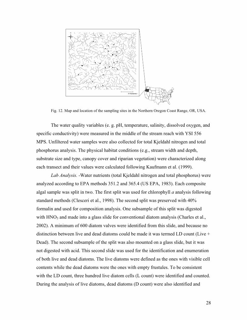
28

Fig. 12. Map and location of the sampling sites in the Northern Oregon Coast Range, OR, USA.

The water quality variables (e. g. pH, temperature, salinity, dissolved oxygen, and

specific conductivity) were measured in the middle of the stream reach with YSI 556

MPS. Unfiltered water samples were also collected for total Kjeldahl nitrogen and total

phosphorus analysis. The physical habitat conditions (e.g., stream width and depth,

substrate size and type, canopy cover and riparian vegetation) were characterized along

each transect and their values were calculated following Kaufmann et al. (1999).

Lab Analysis. -Water nutrients (total Kjeldahl nitrogen and total phosphorus) were

analyzed according to EPA methods 351.2 and 365.4 (US EPA, 1983). Each composite

algal sample was split in two. The first split was used for chlorophyll a analysis following

standard methods (Clesceri et al., 1998). The second split was preserved with 40%

formalin and used for composition analysis. One subsample of this split was digested

with HNO3 and made into a glass slide for conventional diatom analysis (Charles et al.,

2002). A minimum of 600 diatom valves were identified from this slide, and because no

distinction between live and dead diatoms could be made it was termed LD count (Live +

Dead). The second subsample of the split was also mounted on a glass slide, but it was

not digested with acid. This second slide was used for the identification and enumeration

of both live and dead diatoms. The live diatoms were defined as the ones with visible cell

contents while the dead diatoms were the ones with empty frustules. To be consistent

with the LD count, three hundred live diatom cells (L count) were identified and counted.

During the analysis of live diatoms, dead diatoms (D count) were also identified and

29

enumerated. The L and D counts from the second slide were used to calculate the

percentages of live and dead diatoms. All diatoms were identified to the lowest possible

taxonomic level (mainly species) at 1000x magnification, using Leica DM LB2 light

microscope with differential interference contrast (DIC). The diatom taxonomy followed

predominantly Krammer and Lange-Bertalot (1997 a, 1997 b, 2000, 2004) and Patrick

and Reimer (1966, 1975).

Data analysis. - Diatom counts were represented as relative abundances. To

compare the three assemblages (LD, L and D) I will calculate species richness, relative

abundance of dominant species, similarity between samples and site ordinations. Species

richness and the relative abundances of the dominant species will be evaluated with

paired t-tests due to their dependent nature. The similarity among the three assemblages

for each stream site will be assessed using Bray-Curtis similarity coefficient. Bray-Curtis

similarity values range between 0 (complete difference) and 100 (complete similarity).

The Bray-Curtis similarities will be used in non-metric multidimensional scaling

ordination (NMDS) to project their relationships into a low-dimensional space and to best

preserve the ranked distances between them. NMDS does not require any assumptions

about the species distribution, and allows for user-specified distance measure. NMDS

will be run separately for LD, L and D assemblages. The resulting three NMDS plots will

be compared using procrustes analysis with permutation test (Gower, 1971; Peres-Neto

and Jackson, 2001). Procrustes analysis rotates two ordinations to maximize the

similarities between them by minimizing the sum of their squared distances (m2 statistic,

Gower, 1971). Higher values of the m2 statistic indicate better correspondence between

two ordinations. To explore the relationship of each assemblage with its environment, a

linear fitting function will be used. This function finds vector averages of the

environmental variables, and fits them in the ordination space defined by the species data.

All data analyses will be performed using R language and environment for statistical

computing (R Development Core Team, 2008).

Preliminary results

The sampled stream reaches were generally small and well-shaded (Table 4).

Most streams were narrower than 7.0 m, but their stream width ranged from 1.9 to 10.1

m. The streams were shallow, with a mean depth of 4.0 to 14.8 cm. Mid-channel

30

canopy cover ranged between 50-100% with an average of 90%. The water temperature

ranged from 9.5 to 13.0oC, and pH was slightly acidic to neutral (range 5.5 to 7.5). All

streams had very low nutrient levels. The mean value of chlorophyll a was 0.025 mg/m2.

Watershed area ranged between 2.4 and 23.7 km2.

Table. 4. Minimum, mean and maximum values for some environmental variables for Oregon Coast Range streams (n=25). Min Mean Max Algal biomass Chlorophyll (mg/m2) 0.01 0.03 0.06 Water quality pH 5.5 6.9 7.5 Temperature (Co) 9.5 11.2 13.1 Specific conductivity (µS/cm) 41.0 68.2 203.0 Total phosphorus (mg/L) 0.01 0.02 0.05 Total Kjeldahl nitrogen (mg/L) 0.01 0.03 0.07 Physical habitat Watershed area (km2) 2.4 9.8 23.7 Mean depth (cm) 4.1 8.7 14.8 Mean wetted width (m) 1.9 4.6 10.2 Canopy cover (%) 50.0 89.5 99.7 Riparian deciduous canopy (%) 0.0 70.4 100.0 Riffles (%) 33.3 70.7 88.9 Smooth bedrock (%) 0.0 6.4 31.1 Fine gravel (%) 0.0 9.2 28.9 Sand (%) 0.0 3.2 13.6 Fines (Silt/Clay/Muck) (%) 0.0 3.5 37.8

A total of 135 species were recorded in the LD counts, with a mean species

richness of 26 (Table 5). Fewer taxa (90) were identified in the L counts, with mean

species richness of 19. The D counts were slightly more diverse than the L ones with a

total of 96 species, and a mean species richness of 20. There were 47, 7 and 12 species

unique to the LD, L and D counts, respectively, occurring with less than 1% mean

relative abundance.

31

Table. 5. Community characteristics with mean (minimum and maximum) values. LD L D Total number of species 135 90 96 Sample richness 26 (13-50) 19 (10-42) 20 (11-40) Dominant species (% relative abundance) Achnanthidium minutissimum (Kütz.) Cz. 23.0 (1.5-85.0) 28.0 (3.7-89.0) 25.1 (2.3-76.6) Rhoicosphenia abbreviata (Ag.) L.-B. 16.3 (0-57.2) 12.1 (0-56.0) 8.7 (0-27.2) Achnanthidium deflexum (Reim.) King. 9.0 (0.3-43.0) 11.6 (0.5-50.0) 9.4 (0.4-43.3) Planothidium lanceolatum (Bréb.) L.-B. 8.2 (0-26.0) 5.6 (0-25.0) 9.3 (0-29.5) Cocconeis placentula Ehr. 8.0 (0.5-40.0) 4.6 (0-23.0) 8.7 (0.3-40.0) Gomphonema pumilum (Grun.)R. & L.-B. 7.8 (0.8-40.2) 7.1 (0.3-50.5) 8.5 (1.6-37.2) Nitzschia inconspicua Grun. 5.2 (0-32.0) 7.0 (0-50.0) 7.1 (0-43.0) Mean % dominance by 1 taxon 39.8 43.7 36.5

The mean percentage of live diatoms in a sample was 63.4% (range 50.5-79.4).

The assemblages were overall similar. Their mean similarity values were 72.4%, 73.4%

and 75.4% for LD and L, L and D, and LD and D, respectively.

Time Table

Winter 2009 data analysis, dissertation writing

Spring 2009 dissertation defense

References:

Acker, F. 2002. Analysis of soft-algae and enumeration of total number of diatoms in USGS NAWQA

program quantitative targeted-habitat (RTH and DTH) samples. Protocol P-13-63 in Charles, D.F.,

C. Knowles & R. S. Davis. (Eds.), Protocols for the analysis of algal samples collected as part of

the U.S. Geological Survey National Water-Quality Assessment Program. Report No. 02-06,

Patrick Center for Environmental Research, The Academy of Natural Sciences, Philadelphia, PA.

(URL http://diatom.acnatsci.org/nawqa/pdfs/ProtocolPublication.pdf)

Alverson, A. J., K. M. Manoylov and R. J. Stevenson. 2003. Laboratory sources of error for algal

community attributes during sample preparation and counting. Journal of Applied Phycology 15:

357-369.

Bahls, L.L. 1993. Periphyton bioassessment methods for Montana streams. Water Quality Bureau,

Department of Health and Environmental Sciences, Helena, MT.

Barbour, M. T., J. Gerritsen, G. E. Griffith, R. Frydenborg, E. Mccarron, J. S. White and M. L. Bastian.

1996. A framework for biological criteria for Florida streams using benthic macroinvertebrates.

Journal of the North American Benthological Society 15 (2): 185-211.

32

Barbour, M.T., J. Gerritsen, B.D. Snyder and J.B. Stribling. 1999. Rapid bioassessment protocols for use in

streams and wadeable rivers: periphyton, benthic macroinvertebrates, and fish. Second edition.

EPA 841-B-99-002. US Environmental Protection Agency. Washington, DC.

Biggs, B. J. F. 1996. Patterns of benthic algae in streams. Pp. 31-76 in R. J. Stevenson, M. L. Bothwell and

R. L. Lowe (Eds.), Algal ecology: freshwater benthic ecosystems. Academic Press, San Diego,

California.

Cao, Y., D. D. Williams and N. E. Williams. 1998. How important are rare species in aquatic community

ecology and bioassessment? Limnology and Oceanography 43 (7): 1403-1409.

Cao, Y. and D. D. Williams. 1999. Rare species are important in bioassessment (reply to the comment by

Marchant). Limnology and Oceanography 44 (7): 1841-1842.

Cao, Y., D. P. Larsen, and R. St-J. Thorne. 2001. Rare species in multivariate analysis for bioassessment:

some considerations. Journal of the North American Benthological Society 20: 144–153.

Carlisle, D. M., C. P. Hawkins, M. R. Meador, M. Potapova and J. Falcone. 2008. Biological assessments

of Appalachian streams based on predictive models for fish, macroinvertebrate, and diatom

assemblages. Journal of the North American Benthological Society 27 (1): 16-37.

Charles, D.F., C. Knowles and R. S. Davis. 2002. Protocols for the analysis of algal samples collected as

part of the U.S. Geological Survey National Water-Quality Assessment Program. Report No. 02-

06, Patrick Center for Environmental Research, The Academy of Natural Sciences, Philadelphia,

PA. (URL http://diatom.acnatsci.org/nawqa/).

CLAMS (Coastal landscape analysis and modeling study). 1996. (URL

http://www.fsl.orst.edu/clams/data_index.html).

Clarke, K. R. 1993. Non-parametric multivariate analyses of changes in community structure. Australian

Journal of Ecology 18: 117-143.

Clarke, S. E., D. White & A. L. Schaedel. 1991. Oregon, USA, Ecological regions and subregions for water

quality management. Environmental Management 15: 847-856.

Clesceri, L. S., A. E. Greenberg & A. D. Eaton. 1998. Standard Methods for the Examination of Water and

Wastewater, 20th Edition. American Public Health Association, Washington, DC.

Cox, E. J. 1996. Identification of freshwater diatoms from live material. Chapman & Hall, London, UK.

Cox, E. J. 1998. A rationale and some suggestions for developing rapid biomonitoring techniques using

identification of live diatoms. Proceedings of the 15th International Diatom Symposium: 43-50.

Davies , S. P. and S. K. Jackson. 2006. The biological condition gradient: a descriptive model for

interpreting change in aquatic ecosystems. Ecological Applications 16(4): 1251–1266.

Dickman, M. 1968. The effect of grazing by tadpoles on the structure of a periphyton community. Ecology

49 (6): 1188-1190.

Faith, D. P. and R. H. Norris.1989. Correlation of environmental variables with patterns of distribution and

abundance of common and rare freshwater macroinvertebrates. Biological Conservation 50 (1):

77-98.

33

Fore, L. S. 2002. Response of diatom assemblages to human disturbance: development and testing of a

multimetric index for the Mid-Atlantic Region (USA). Pp. 445-480 in T. P. Simon (Ed.),

Biological response signatures: patterns in biological integrity for assessment of freshwater

aquatic assemblages. CRC Press LLC, Boca Raton, FL.

Fore, L.S., J.R. Karr and L.L. Conquest. 1994. Statistical properties of an index of biotic integrity used to

evaluate water resources. Canadian Journal of Fisheries and Aquatic Sciences 51: 1077-1087.

Fore, L.S., J.R. Karr and R.W. Wisseman. 1996. Assessing invertebrate responses to human activities:

evaluating alternative approaches. Journal of the North American Benthological Society 15: 212-

231.

Gaston, K. J. 1994. Rarity. Chapman & Hall, London.

Gotelli, N. J. and A. M. Ellison. 2004. A primer of ecological statistics. Sinauer Associates, Inc.,

Sunderland, Massachusetts, USA.

Gower, J. C. 1971. Statistical methods of comparing different multivariate analyses of the same data. Pp.

138–149 in Hodson, F.R., D.G. Kendall and P. Tautu (Eds.), Mathematics in the archaeological

and historical sciences. Edinburgh University Press.

Grinnell, J. 1917. The niche-relationships of the California Thrasher. Auk 34: 427-433.

Hassan, G. S., M. A. Espinosa and F. I. Isla. 2008. Fidelity of dead diatom assemblages in estuarine

sediments: how much environmental information is preserved? Palaios 23: 112-120.

Hawkins, C. P., R. H. Norris, J. N. Hogue and J. W. Feminella. 2000. Development and evaluation of

predictive models for measuring the biological integrity of streams. Ecological Applications 10

(5): 1456-1477.

Herlihy, A.T. 2006. Water chemistry. Pp. 73-84 in Peck, D.V., A. T. Herlihy, B. H. Hill, R. M. Hughes, P.

R. Kaufmann, D. Klemm, J. M. Lazorchak, F. H. McCormick, S. A. Peterson, P. L. Ringold, T.

Magee and M. Cappaert (Eds.), Environmental Monitoring and Assessment Program -Surface

Waters: Western Pilot Study Field Operations Manual for Wadeable Streams. EPA/620/R-06/003.

Office of Research and Development, U.S. Environmental Protection Agency, Washington, D.C.

Herlihy, A. T., D. P. Larsen, S. G. Paulsen, N. S. Urquhart and B. J. Rosenbaum. 2000. Designing a

spatially balanced, randomized site selection process for regional stream surveys: the EMAP mid-

Atlantic pilot study. Environmental Monitoring and Assessment 63 (1): 95-113.

Hill, B. H., A. T. Herlihy, P. R. Kaufman, R. J. Stevenson, F. H. Mccormick and C. B. Johnson. 2000. Use

of periphyton assemblage data as an index of biotic integrity. Journal of the North American

Benthological Society 19: 50–67.

Hoagland, K. D., S. C. Roemer and J. R. Rosowski. 1982. Colonization and community structure of two

periphyton assemblages, with emphasis on the diatoms (Bacillariophyceae). American Journal of

Botany 69 (2): 188-213.

Hughes, R. M., D. P. Larsen, and J. M. Omernik. 1986. Regional reference sites: a method for assessing

stream potentials. Evironmental Management 10:629–635.

34

Hughes, R. M. and D. V. Peck. 2008. Acquiring data for large aquatic resource surveys: the art of

compromise among science, logistics, and reality. Journal of the North American Benthological

Society 27 (4): 837–859.

Hughes, R. M., S. G. Paulsen and J. L. Stoddard. 2000. EMAP-Surface Waters: a national,

multiassemblage, probability survey of ecological integrity. Hydrobiologia 423: 429-443.

Hutchinson, G. E. 1957. Concluding remarks. Cold Spring Harbor Symposia on Quantitative Biology 22:

415-427.

Jackson, P. L. and A. J. Kimerling 1993. Atlas of the Pacific Northwest. OSU Press, Corvallis, OR.

Karr, J.R. 1981. Assessment of biotic integrity using fish communities. Fisheries 6 (6): 21-27.

Karr, J. R. 1991. Biological integrity: a long-neglected aspect of water resource management. Ecological

Applications 1: 66-84.

Karr, J. R. 1999. Defining and measuring river health. Freshwater Biology 41 (2): 221-234.

Karr, J. R. and E.W. Chu. 1999. Restoring life in running waters: better biological monitoring. Island

Press, Washington, D.C.

Kaufmann, P. R. 2006. Physical habitat characterization. Pp. 97-153 in Peck, D.V., A. T. Herlihy, B. H.

Hill, R. M. Hughes, P. R. Kaufmann, D. Klemm, J. M. Lazorchak, F. H. McCormick, S. A.

Peterson, P. L. Ringold, T. Magee and M. Cappaert (Eds.), Environmental Monitoring and

Assessment Program -Surface Waters: Western Pilot Study Field Operations Manual for

Wadeable Streams. EPA/620/R-06/003. Office of Research and Development, U.S. Environmental

Protection Agency, Washington, D.C.

Kaufmann, P. R, P. Levine, E.G. Robison, C. Seeliger and D.V. Peck. 1999. Quantifying Physical Habitat

in Wadeable Streams. EPA/620/R-99/003. U.S. Environmental Protection Agency, Washington,

D.C.

Kelly, M. 2001. Use of similarity measures for quality control of benthic diatom samples. Water Resources

35: 2784-2788.

Kelly, M. G. and B. A. Whitton. 1995. Trophic diatom index - a new index for monitoring eutrophication in

rivers. Journal of Applied Phycology, 7 (4): 433-444.

Kerans, B.L. and J.R. Karr. 1994. A benthic index of biotic integrity (B-IBI) for rivers of the Tennessee

Valley. Ecological Applications 4: 768-785.

Korte, V. L. and D. W. Blinn. 1983. Diatom colonization on artificial substrata in pool and riffle zones

studied by light and scanning electron microscopy. Journal of Phycology 19 (3): 332-341.

Krammer K. & Lange-Bertalot H. 1986. 1988, 1991a, b. Bacillariophyceae. In J. Ettl, J. Gerloff, H. Heynig

and D. Mollenhauer (Eds), Sußwasserflora von Mitteleuropa 2/1-2/4. G. Fisher, Stuttgart.

Lange-Bertalot, H. 1979. Pollution tolerance of diatoms as a criterion for water quality estimation. Nova

Hedwigia 64:285–303.

35

Lavoie, I., P. J. Dillon and S. Campeau. 2009. The effect of excluding diatom taxa and reducing taxonomic

resolution on multivariate analyses and stream bioassessment. Ecological Indicators 9 (2): 213-

225.

Lazorchak, J.M., D.J. Klemm & D.V. Peck. 1998. Environmental Monitoring and Assessment Program -

Surface Waters: Field Operations and Methods for Measuring the Ecological Condition of

Wadeable Streams. EPA/620/R-94/004F. U.S. Environmental Protection Agency, Washington,

D.C.

Leibold, M. A. 1995. The niche concept revisited: mechanistic models and community context. Ecology 76

(5): 1371-1382.

MacArthur, R. and R. Levins. 1967. The limiting similarity, convergence, and divergence of coexisting.

The American Naturalist 101: 377-385.

Magurran, A. E. 2004 Measuring biological diversity. Wiley-Blackwell.

Marchant, R. 1999. How important are rare species in aquatic community ecology and bioassessment? A

comment on the conclusions of Cao et al. Limnology and Oceanography 44 (7): 1840-1841.

Marchant, R. 2002. Do rare species have any place in multivariate analysis for bioassessment? Journal of

the North American Benthological Society 21 (2): 311–313.

Marchant, R., A. Hirst, R. H. Norris, R. Butcher, L. Metzeling and D. Tiller. 1997. Classification and

ordination of macroinvertebrate assemblages from running waters in Victoria, Australia. Journal

of the North American Benthological Society 16: 664–681.

Mccormick, P. V. and R. J. Stevenson. 1991. Mechanisms of benthic algal succession in lotic

environments. Ecology 72 (5): 1835-1848.

Miller, A. R., R. L. Lowe and J. T. Rotenberry. 1987. Succession of diatom communities on sand grains.

The Journal of Ecology 75 (3): 693-709.

Naiman, R. J. & R. E. Bilby. 1998. River ecology and management in the Pacific Coastal ecoregion. Pp. 1-

10 in Naiman, R. J. & R. E. Bilby (Eds.), River ecology and management: lessons from the Pacific

Coastal ecoregion. Springer-Verlag, New York.

Nijboer, R. C. and A. Schmidt-Kloiber. 2004. The effect of excluding taxa with low abundances or taxa

with small distribution ranges on ecological assessment. Hydrobiologia 516 (1): 347-363.

Odum, E. P. 1985. Trends expected in stressed ecosystems. Bioscience 35 (7): 419-422.

Omernik, J.M. 1987. Ecoregions of the conterminous United States. Annals of the Association of American

Geographers 77:118-125.

Oppenheim, D. R. 1987. Frequency distribution studies of epipelic diatoms along an intertidal shore.

Helgoland Marine Research 41: 139-148.

Owen, B. B., M. Afzal and W. R. Cody. 1979. Distinguishing between live and dead diatoms in periphyton

communities. Pp. 70-76 in Wetzel, R. L. (Ed.), Methods and measurements of periphyton

communities: a review. American Society for Testing and Materials, STP 690.

36

Pan, Y., R. J. Stevenson, B. H. Hill, A. T. Herlihy, and C. B. Collins. 1996. Using diatoms as indicators of

ecological conditions in lotic systems: a regional assessment. Journal of the North American

Benthological Society 15: 481-494.

Pan, Y. D., R. J. Stevenson, B. H. Hill, P. R. Kaufmann and A. T. Herlihy. 1999. Spatial patterns and

ecological determinants of benthic algal assemblages in Mid-Atlantic streams, USA. Journal of

Phycology 35(3): 460-468.

Pan, Y. D., R. J. Stevenson, B. H. Hill and A. T. Herlihy. 2000. Ecoregions and benthic diatom

assemblages in Mid-Atlantic Highlands streams, USA. Journal of the North American

Benthological Society 19(3): 518-540.

Patrick, R. 1967. The effect of invasion rate, species pool, and size of area on the structure of the diatom

community. Proceedings of the National Academy of Sciences 58: 1335-1342.

Patrick, R. 1973. Use of algae, especially diatoms, in the assessment of water quality. Pp. 76-95 in Cairns,

J. Jr. and K. L. Dickson (Eds.), Biological Methods for the Assessment of Water Quality. ASTM

STP 528, American Society for Testing and Materials, Philadelphia, PA, USA.

Patrick, R. 1976. The formation and maintenance of benthic diatom communities. Proceedings of the

American Philosophical Society 120 (6): 475-484.

Patrick, R., M. H. Hohn and J. H. Wallace. 1954. A new method for determining the pattern of the diatom

flora. Notulae Naturae of the Academy of Natural Sciences of Philadelphia 259: 1-12.

Patrick, R. & C. W. Reimer. 1966. The Diatoms of the United States. Vol. 1. Monograph #13 of the

Academy of Natural Sciences of Philadelphia.

Patrick, R. & C. W. Reimer. 1975. The Diatoms of the United States. Vol. 2. Monograph #13 of the

Academy of Natural Sciences of Philadelphia.

Paulsen, S. G., A. Mayio, D. V. Peck, J. L. Stoddard, E. Tarquinio, S. M. Holdsworth, J. Van Sickle, L.

L. Yuan, C. P. Hawkins, A. T. Herlihy, P. R. Kaufmann, M. T. Barbour, D. P. Larsen and A.

R. Olsen. 2008. Condition of stream ecosystems in the US: an overview of the first national

assessment. Journal of the North American Benthological Society 27 (4): 812–821.

Peck, D.V., A. T. Herlihy, B. H. Hill, R. M. Hughes, P. R. Kaufmann, D. Klemm, J. M. Lazorchak, F. H.

McCormick, S. A. Peterson, P. L. Ringold, T. Magee and M. Cappaert. 2006. Environmental

Monitoring and Assessment Program -Surface Waters: Western Pilot Study Field Operations

Manual for Wadeable Streams. EPA/620/R-06/003. Office of Research and Development, U.S.

Environmental Protection Agency, Washington, D.C.

Peres-Neto, P.R. & D.A. Jackson. 2001. How well do multivariate data sets match? The advantages of a

Procrustean superimposition approach over the Mantel test. Oecologia 129: 169–178.

Peterson, C. G. 1987. Gut passage and insect grazer selectivity of lotic diatoms. Freshwater Biology 18 (3):

455-460.

Peterson, C.G. 1996. Mechanisms of lotic microalgal colonization following space-clearing disturbances

acting at different spatial scales. Oikos 77 (3): 417-435.

37

Peterson, C. G. and Stevenson, R. J. 1989. Substratum conditioning and diatom colonization in different

current regimes. Journal Of Phycology 25 (4): 790-793.

Peterson, C. G., K. D. Hoagland and R. J. Stevenson. 1990. Timing of wave disturbance and the resistance

and recovery of a freshwater epilithic microalgal community. Journal of the North American

Benthological Society 9 (1): 54-67.

Peterson, C. G. and R. J.Stevenson. 1992. Resistance and resilience of lotic algal communities -

importance of disturbance timing and current. Ecology 73 (4): 1445-1461.

Potapova, M. G. and D. F. Charles. 2002. Benthic diatoms in USA rivers: distributions along spatial and

environmental gradients. Journal of Biogeography 29 (2): 167-187.

Potapova, M. and D. F. Charles. 2003. Distribution of benthic diatoms in US rivers in relation to

conductivity and ionic composition. Freshwater Biology 48 (8): 1311-1328.

Potapova, M. and D. F. Charles. 2004. Potential use of rare diatoms as environmental indicators in USA

rivers. Pp. 281-295 in M Poulin (Ed.), Proceedings of the 17th International diatom symposium.

Biopress Ltd., Bristol.

Potapova, M. and D. F. Charles. 2005. Choice of substrate in algae-based water-quality assessment. Journal

of the North American Benthological Society 24 (2): 415-427.

Pryfogle, P. A. 1975. Seasonal distribution of periphytic diatom communities of Tymochtee Creek. In

Proceedings of the Sandusky River Basin Symposium. International Joint Commission Canada-

U.S.A. Great Lakes Water Quality Agreement 1972: 153–173.

Pryfogle, P. A. & R. L. Lowe. 1979. Sampling and interpretation of epilithic lotic diatom communities. Pp.

77-89 in Wetzel, R. L. (Ed.), Methods and measurements of periphyton communities: a review.

American Society for Testing and Materials, STP 690.

Prygiel, J., P. Carpentier, S. Almeida, M. Coste, J.-C. Druart, L. Ector, D. Guillard, M.-A. Honoré, R.

Iserentant, P. Ledeganck, C. Lalanne-Cassou, C. Lesniak, I. Mercier, P. Moncaut, M. Nazart, N.

Nouchet, F. Peres, V. Peeters, F. Rimet, A. Rumeau, S. Sabater, F. Straub, M. Torrisi, L.

Tudesque, B. V. de Vijver, H. Vidal, J. Vizinet & N. Zydek. 2002. Determination of the biological

diatom index (IBD NF T 90–354): results of an intercomparison exercise. Journal of Applied

Phycology 14: 27-39.

Rabinowitz, D. 1981. Seven forms of rarity. pp. 205-217 in The biological aspects of rare plant

conservation. H. Synge (Ed.), John Wiley, Chichester, UK.

Reisen, W. K. and D. J. Spencer. 1970. Succession and current demand relationships of diatoms on

artificial substrates in Prater's Creek, South Carolina, Journal of Phycology 6 (2): 117-121.

Reynoldson, T. B., R. C. Bailey, K. E. Day and R. H. Norris. 1995. Biological guidelines for fresh- water

sediment based on BEnthic Assessment of SedimenT (the BEAST) using a multivariate approach

for predicting biological state. Australian Journal of Ecology 20: 198-219.

Ripley, B.D. 1996. Pattern recognition and neural networks. Cambridge, Cambridge University Press.

38

Round, F. E. 1998. A problem in algal ecology: contamination of habitats from adjacent communities.

Cryptogamie Algologie 19: 49-55.

R Development Core Team. 2008. R: a language and environment for statistical computing. R Foundation

for Statistical Computing, Vienna, Austria. (URL http://www.R-project.org).

Sawai, Y. 2001. Distribution of living and dead diatoms in tidal wetlands of northern Japan: relations to

taphonomy. Palaeogeography, Palaeoclimatology, Palaeoecology 173: 125–141.

Steinman, A. D. and C. D. McIntire. 1986. Effects of current velocity and light energy on the structure of

periphyton assemblages in laboratory streams. Journal of Phycology 22: 352-361.

Steinman, A. D., C. D. McIntire, S. V. Gregory, G. A. Lamberti and L. R. Ashkenas. 1987. Effects of

herbivore type and density on taxonomic structure and physiognomy of algal assemblages in

laboratory streams, Journal of the North American Benthological Society 6 (3): 175-188.

Steinman, A. D. and C. D. McIntire. 1990. Recovery of lotic periphyton communities after disturbance.

Environmental Management 14 (5): 589-604.

Stevenson, RJ. 1984. Epilithic and epipelic diatoms in the Sandusky river, with emphasis on species-

diversity and water-pollution. Hydrobiologia 114 (3): 161-175.

Stevenson, R. J. 1996. An introduction to algal ecology in freshwater benthic habitats. Pp. 3-30 in

Stevenson, R. J., M. L. Bothwell and Rex L. Lowe (Eds.), Algal Ecology: Freshwater Benthic

Ecosystems, Academic Press, San Diego, CA.

Stevenson, R. J. 1997. Scale-dependent determinants and consequences of benthic algal heterogeneity.

Journal of the North American Benthological Society 16 (1): 248-262.

Stevenson, R. J. 2006. Refining diatom indicators for valued ecological attributes and development of

water quality criteria. Pp. 365-383 in Nadja Ognjanova-Rumenova and Kalina Manoylov (Eds.),

Advances in phycological studies, Pensoft, Sofia-Moscow.

Stevenson, R. J. and C. G. Peterson. 1991. Emigration and immigration can be important determinants of

benthic diatom assemblages in streams. Freshwater Biology 26 (2): 279-294.

Stevenson, R. J. and L. L. Bahls. 1999. Periphyton protocols. Pp 6-1 to 6-22 in: M. T. Barbour, J. Gerritsen,

& B. D. Snyder (Eds.), Rapid bioassessment protocols for use in wadeable streams and rivers:

periphyton, benthic macroinvertebrates, and fish. Second edition. EPA 841-B-99-002 United

States Environmental Protection Agency, Washington, DC.

Stevenson, R. J., C. G. Peterson, D. B. Kirschtel, C. C. King, and N. C. Tuchman. 1991. Density-dependent

growth, ecological strategies, and effects of nutrients and shading on benthic diatom succession in

streams. Journal of Phycology 27 (1): 59-69.

Stevenson, R. J. and Y. Pan. 1999. Assessing ecological conditions in rivers and streams with diatoms. Pp.

11-40 in E. F. Stoermer and J. P. Smol (Eds.), The diatoms: applications to the environmental and

earth sciences.. Cambridge University Press, Cambridge, UK.

Stoddard, J. L., D. V. Peck, S. G. Paulsen, J. Van Sickle, C. P. Hawkins, A. T. Herlihy, R. M. Hughes, P. R.

Kaufmann, D. P. Larsen, G. Lomnicky, A. R. Olsen, S. A. Peterson, P. L. Ringold and T. R.

39

Whittier. 2005. An ecological assessment of western streams and rivers. EPA 620/R-05/005, U.S.

Environmental Protection Agency, Washington, DC.

Stoddard, J. L., D. P. Larsen, C. P. Hawkins, R. K. Johnson and R. H. Norris. 2006. Setting expectations for

the ecological condition of streams: the concept of reference condition. Ecological Applications 16

(4): 1267-1276.

Suter II, G. W. 1993. A critique of ecosystem health concepts and indexes. Environmental Toxicology and

Chemistry 12 (9): 1533–1539.

Ter Braak, C. J. F. and C. W. N. Looman. 1986. Weighted averaging, logistic regression and the Gaussian

response model. Vegetatio 65: 3-11.

Thomas, D. P. 1979. Some problems connected with the use of cleared cells and relative proportions of

species in diatom ecology. Beiheft für Nova Hedwigia 64: 503-511.

US EPA. 1983. Methods for chemical analysis of water and wastes. EPA-600/4-79-020. U.S.

Environmental Protection Agency, Cincinnati, OH.

US EPA. 1989. Handbook of methods for acid deposition studies: field operations for surface water

chemistry. EPA 600/4-89/020. U.S. Environmental Protection Agency, Office of Research and

Development, Washington, D.C.

US EPA. 1996. Summary of state biological assessment programs for streams and rivers. EPA 230-R-96-

007. U.S. Environmental Protection Agency, Office of Policy, Planning, and Evaluation,

Washington, DC.

US EPA. 2002. Summary of biological assessment programs and biocriteria development for states, tribes,

territories, and interstate commissions: streams and wadeable rivers. EPA-822-R-02-048. U.S.

Environmental Protection Agency, Office of Environmental Information and Office of Water,

Washington, D.C.

Vannote, R. L., G. W. Minshall, K. W. Cummins, J. R. Sedell and C. E. Cushing. 1980. The river

continuum concept. Canadian Journal of Fisheries and Aquatic Sciences 37: 130-137.

Van Sickle, J., D. P. Larsen and C. P. Hawkins. 2007. Exclusion of rare taxa affects performance of the

O/E index in bioassessments. Journal of the North American Benthological Society 26 (2): 319–

331.

Walker, G. W. & N. S. MacLeod. 1991. Geologic map of Oregon. US Geological Survey, scale 1:500,000.

(URL http://geopubs.wr.usgs.gov/docs/geologic/or/oregon.html)

Weilhoefer, C. L. & Y. Pan. 2007. A comparison of periphyton assemblages generated by two sampling

protocols. Journal of the North American Benthological Society 26: 308-318.

Whittier, T. R., J. L. Stoddard, D. P. Larsen and A. T. Herlihy. 2007. Selecting reference sites for stream

biological assessments: best professional judgment or objective criteria. Journal of the North

American Benthological Society 26 (2): 349-360.

Wilson, C. J. & R. W. Holmes. 1981. The ecological importance of distinguishing between living and dead

diatoms in estuarine sediments. European Journal of Phycology 16: 345 – 349.

40

Wright, J.F., D.W. Sutcliffe, and M.T. Furse., 2000. Assessing the biological quality of fresh waters:

RIVPACS and other techniques. Freshwater Biological Association, Ambleside, Cumbria,

England.