DG-FEM for PDE’s Lecture 7 - Technical University of …apek/DGFEMCourse2009/Lecture07.pdf · DG-FEM for PDE’s Lecture 7 ... Introduction and DG-FEM in 1D • Lecture 2: Implementation

Jan S HesthavenBrown [email protected]

DG-FEM for PDE’sLecture 7

DGFEM 2009

mailto:[email protected]

mailto:[email protected]

A brief overview of what’s to come

• Lecture 1: Introduction and DG-FEM in 1D

• Lecture 2: Implementation and numerical aspects

• Lecture 3: Insight through theory

• Lecture 4: Nonlinear problems

• Lecture 5: Extension to two spatial dimensions

• Lecture 6: Introduction to mesh generation

• Lecture 7: Higher order/Global problems

• Lecture 8: 3D and advanced topics

Lecture 7

✓ Let’s briefly recall what we know

✓ Brief overview of multi-D analysis

✓ Part I: Time-dependent problems

✓ Heat equations

✓ Extensions to higher order problems

✓ Part II: Elliptic problems

✓ Different formulations

✓ Stabilization

✓ Solvers and application examples

Lets summarizeWe have a thorough understanding of 1st order problems

✓ For the linear problem, the error analysis and convergence theory is essentially complete. ✓ The theoretical support for DG for conservation laws is very solid.✓ Limiting is perhaps the most pressing open problem✓ The extension to 2D is fairly straightforward✓ .... and we have a nice and flexible way to implement it all

Time to move beyond the 1st order problem

Brief overview of multi-D analysis

In 1D we discussed that

6.7 A few theoretical results 237

In later work [190], this result was improved to

!u " uh!!,h # ChN+1/2!u!!,N+1,h,

provided the triangulation is quasi-uniform in the sense that the angles in alltriangles are bounded from below by a constant independent of the elementsize, h. In [190], much broader results were obtained also, including errorestimates in general Lp-norms.

It remained unclear, however, whether this result in L2 was sharp or simplya result of the analysis. In [272], this result was further improved to the optimalresult

!u " uh!!,h # ChN+1!u!!,N+2,h,

provided the grid is quasi-uniform and that all edges are bounded away fromthe characteristic direction (i.e., |!·n| > 0 for all outward pointing normals onthe element edges). In other words, this analysis does not capture the specialcase where edges are aligned with the characteristic direction.

To understand whether there are potential problems in this special case,let us consider an example, taken from [257].

Example 6.4. Consider the special case of the neutron equation as

!u

!y= 0, x $ [0, 1]2,

and withu(x, 0) = x.

It is easy to see that the exact solution is u(x, y) = x.We now assume that " = [0, 1]2 is triangulated using a simple grid where

hx = h = 1/I and hy = h/2 with I being the number of cells along x. In otherwords, the edge length along x is twice that along y, but otherwise the gridis entirely regular.

To solve the problem, we will use the simplest possible formulation, basedon an N = 0 basis; that is, it is a finite volume method given on the cellwiseform !

!Dknyu! dx = 0.

Using upwinding and exploiting the geometry of the grid, it is easy to see thatthe local scheme is

ui,j+1 =12

"ui"1/2,j + ui+1/2,j

#,

where we have defined the grid function

ui,j = uh

$ih,

jh2

%for

&i = 1/2, 3/2, 5/2, . . . , I ! 1/2, j = 0, 2, 4, . . . , Ji = 0, 1, 2, . . . , I, j = 1, 3, 5, . . . , J ! 1.

.. but this was a somewhat special case.

Question is -- is it possible in multi-D ?

Answer - No

238 6 Beyond one dimension

Induction now allows one to write down the exact numerical solution as

ui,j =12j

j!

q=0

"jq

#uj/2!q+i,0 =

12j

j!

q=0

"jq

#|h(j/2 ! q + i)|,

since u(x, 0) = x.Note that along x = 0 and x = 1, the grid is, by necessity, aligned with the

characteristic direction. Let us therefore consider the solution u0,1!h/2 givenas

u0,J!1 =12j

j!

q=0

"jq

#|h(j/2 ! q)| =

J+1!

j=1,3,5,...

h

2j

"j ! 1

(j ! 1)/2

#,

where we refer to [257] for a derivation of the last reduction. Using Stirling’sformula, we have

"a

a/2

#=

a!(a/2)!(a/2)!

" c2a+1a!1/2,

such that

u0,J!1 " chJ+1!

j=1,3,5,...

1#j ! 1

" ch#

J " ch1/2,

as J $ h!1. Since the exact solution is u(0, y) = 0, this result also reflects thepointwise error and indicates the possibility of losing optimality for certainspecial grids.

The above example reflects that if n ·! = 0, there may be a loss of optimalconvergence rate, at least for N = 0. In [257], this was used to construct aproblem, based on the above example with a grid with many vertical gridlines, which demonstrates the loss of optimality in L2 and confirms that theoriginal result in [190] of

%u ! uh%!,h & ChN+1/2%u%!,N+1,h,

is in fact sharp. It should be emphasized, though, that the suboptimal be-havior should be expected for very specific grids only and one can generallyexpect optimal order for DG-FEM when solving problems with smooth solu-tions on general unstructured grids. Furthermore, for linear problems one cannaturally guarantee that this special case does not happen by constructingthe grid appropriately. This conforms well with what we saw in the exampleof Maxwell’s equations in Section 6.5. The above discussion does not cover thecentral flux and, as we will see in Chapter 7, a loss of optimality in convergencerate is often associated with this choice of flux.

The results in Section 6.6 show that these results, as in the one-dimensionalcase, can be expected to carry over to nonlinear problems with smooth solu-tions as long as monotone fluxes are used. The proof of this for the multidi-mensional case is given in [337, 338], again assuming the use of upwind fluxes.

... but the optimal rate is often observed as initial error dominates over the accumulated error

The heat equation

Let us consider the heat equation

7

Higher-order equations

So far, we have only considered problems with first order spatial derivatives(e.g., as in conservation laws), and shown the methods to perform well and inagreement with the strong theoretical foundation. It is natural to ask whetherone can extend the formulation to include more general problem types. Thisis the topic of this chapter and, as we will see shortly, the generalization todeal with higher-order spatial operators is less direct than one would expect.Let us consider the following simple example, taken from [288].

Example 7.1. Consider the linear heat equation

!u

!t=

!2u

!x2, x ! [0, 2"],

with periodic boundary conditions and u(x, 0) = sin(x). The exact solution iseasily found as

u(x, t) = e!t sin(x).

Based on the previous discussions of the discontinuous Galerkin methods, itis tempting to simply write the heat equation as

!u

!t" !

!xux = 0,

and then identify ux as the flux in the first order equation. The resultingscheme becomes

vkh = Dru

kh, Mk duk

h

dt" Svk

h = "!

!Dkn ·

"vk

h " v"# !k(x) dx,

in each element, k. A reasonable choice for the flux could be a simple centralflux (i.e., v" = {{vh}}) since the heat equation has no preferred direction ofpropagation.

7




!u

!t=

!2u

!x2, x ! [0, 2"],




!u

!t" !

!xux = 0,


vkh = Dru

kh, Mk duk

h

dt" Svk

h = "!

!Dkn ·

"vk

h " v"# !k(x) dx,


7




!u

!t=

!2u

!x2, x ! [0, 2"],




!u

!t" !

!xux = 0,


vkh = Dru

kh, Mk duk

h

dt" Svk

h = "!

!Dkn ·

"vk

h " v"# !k(x) dx,


7




!u

!t=

!2u

!x2, x ! [0, 2"],




!u

!t" !

!xux = 0,


vkh = Dru

kh, Mk duk

h

dt" Svk

h = "!

!Dkn ·

"vk

h " v"# !k(x) dx,


7




!u

!t=

!2u

!x2, x ! [0, 2"],




!u

!t" !

!xux = 0,


vkh = Dru

kh, Mk duk

h

dt" Svk

h = "!

!Dkn ·

"vk

h " v"# !k(x) dx,


We can be tempted to write this as

and then just use our standard approach

Given the nature of the problem, a central flux seems reasonable

The heat equation244 7 Higher-order equations

Table 7.1. Global L2-errors for solving the heat equation using K elements, eachwith a local order of approximation, N , using the scheme in Example 7.1. A ‘–’marks that the algorithm is unstable.

N\K 10 20 40 80 160

1 4.27E-1 4.34E-1 4.37E-1 4.38E-1 4.39E-12 5.00E-1 4.58E-1 4.46E-1 4.43E-1 4.42E-14 1.68E-1 1.37E-1 1.28E-1 1.26E-1 –8 7.46E-3 8.60E-3 – – –

0 1.57 3.14 4.71 6.28!0.8

!0.6

!0.4

!0.2

0

0.2

0.4

0.6

0.8

x

u(x,0.8)

N=1

Exact

N=2

N=4

Fig. 7.1. Computed solutions to the heat equation using the scheme in Example7.1 with K = 80 elements and di!erent orders of approximation.

In Table 7.1 we show the global L2-error (i.e., the error measured in! ·! !,h), under refinement both in K and N . The results are disappointing,displaying both lack of convergence and/or regular instability at high resolu-tions.

To further illustrate the problem, we show the computed solutions inFig. 7.1 for fixed K and increasing values of N . Increasing K yields simi-lar results as expected from Table 7.1.

A careful analysis [335] reveals that the scheme is both inconsistent andweakly unstable, consistent with the results in Table 7.1. The instability isdriven by roundo! errors, which, in combination with the weak nature ofthe instability, explains why one does not observe the instability for somelow-resolution cases in Table 7.1.

244 7 Higher-order equations

Table 7.1. Global L2-errors for solving the heat equation using K elements, eachwith a local order of approximation, N , using the scheme in Example 7.1. A ‘–’marks that the algorithm is unstable.

N\K 10 20 40 80 160

1 4.27E-1 4.34E-1 4.37E-1 4.38E-1 4.39E-12 5.00E-1 4.58E-1 4.46E-1 4.43E-1 4.42E-14 1.68E-1 1.37E-1 1.28E-1 1.26E-1 –8 7.46E-3 8.60E-3 – – –

0 1.57 3.14 4.71 6.28!0.8

!0.6

!0.4

!0.2

0

0.2

0.4

0.6

0.8

x

u(x,0.8)

N=1

Exact

N=2

N=4

Fig. 7.1. Computed solutions to the heat equation using the scheme in Example7.1 with K = 80 elements and di!erent orders of approximation.

In Table 7.1 we show the global L2-error (i.e., the error measured in! ·! !,h), under refinement both in K and N . The results are disappointing,displaying both lack of convergence and/or regular instability at high resolu-tions.

To further illustrate the problem, we show the computed solutions inFig. 7.1 for fixed K and increasing values of N . Increasing K yields simi-lar results as expected from Table 7.1.

A careful analysis [335] reveals that the scheme is both inconsistent andweakly unstable, consistent with the results in Table 7.1. The instability isdriven by roundo! errors, which, in combination with the weak nature ofthe instability, explains why one does not observe the instability for somelow-resolution cases in Table 7.1.

Lets see what happens when we run it

It does not work!

It is weakly unstable

The heat equationWe need a new idea -- consider

7.1 Higher-order time-dependent problems 245

7.1 Higher-order time-dependent problems

From the above example it is clear that a new idea is required to use thediscontinuous Galerkin method for problems with higher spatial derivatives.This new idea, first proposed in [22], is to rewrite the high spatial derivativeas a system of first-order equations; for example, if we need to solve the (well-posed) problem

!u

!t=

P!

p=1

!

!x

"ap

!p!1u

!xp!1

#+ a0u,

subject to suitable boundary conditions, we discretizing the system

!u

!t=

P!

p=1

!apqp!1

!x+ a0u,

with!p = 1, . . . , P " 1 : qp =

!pq

!xp, q0 = u.

At first, this seems to introduce several disadvantages (e.g., the memory us-age increases significantly with the use of the system rather than the scalarformulation). Furthermore, it also appears to be more expensive to evaluatethe spatial derivative using a first-order derivative twice rather than a directlydefined second-order operator.

In the following, we nevertheless pursue this idea in some detail for di!erenttype of problems to illustrate that this overhead is not as bad as it appears ifwe choose the numerical fluxes using certain guidelines. Subsequently, we alsobriefly revisit the issue of computational cost and consider a few special waysof addressing this.

7.1.1 The heat equation

Let us first return to the heat equation discussed in Example 7.1 and followthe idea introduced above. We consider

!u

!t=

!

!xa(x)

!u

!x,

with u = 0 at the outer boundaries. It is easily shown that a(x) > 0 su"cesto guarantee well-posedness. We rewrite this problem as

!u

!t=

!

!x

#aq, q =

#a!u

!x,

to recover a system of first order equations. This we can discretize using thetechniques developed for the conservation laws; that is, we assume that (u, q)can be approximated as


7.1 Higher-order time-dependent problems

From the above example it is clear that a new idea is required to use thediscontinuous Galerkin method for problems with higher spatial derivatives.This new idea, first proposed in [22], is to rewrite the high spatial derivativeas a system of first-order equations; for example, if we need to solve the (well-posed) problem

!u

!t=

P!

p=1

!

!x

"ap

!p!1u

!xp!1

#+ a0u,

subject to suitable boundary conditions, we discretizing the system

!u

!t=

P!

p=1

!apqp!1

!x+ a0u,

with!p = 1, . . . , P " 1 : qp =

!pq

!xp, q0 = u.

At first, this seems to introduce several disadvantages (e.g., the memory us-age increases significantly with the use of the system rather than the scalarformulation). Furthermore, it also appears to be more expensive to evaluatethe spatial derivative using a first-order derivative twice rather than a directlydefined second-order operator.

In the following, we nevertheless pursue this idea in some detail for di!erenttype of problems to illustrate that this overhead is not as bad as it appears ifwe choose the numerical fluxes using certain guidelines. Subsequently, we alsobriefly revisit the issue of computational cost and consider a few special waysof addressing this.

7.1.1 The heat equation

Let us first return to the heat equation discussed in Example 7.1 and followthe idea introduced above. We consider

!u

!t=

!

!xa(x)

!u

!x,

with u = 0 at the outer boundaries. It is easily shown that a(x) > 0 su"cesto guarantee well-posedness. We rewrite this problem as

!u

!t=

!

!x

#aq, q =

#a!u

!x,

to recover a system of first order equations. This we can discretize using thetechniques developed for the conservation laws; that is, we assume that (u, q)can be approximated as

We know that DG is good for 1st order systems.

Since a(x)>0 we can write this as

Now follow our standard approach246 7 Higher-order equations

!u(x, t)q(x, t)

"!

!uh(x, t)qh(x, t)

"=

K#

k=1

!uk

h(x, t)qkh(x, t)

"=

K#

k=1

Np$

i=1

!uk

h(xi, t)qkh(xi, t)

"!ki (x),

where, as usual, we represent (u, q) by N -th-order piecewise polynomials onK elements. We recover the strong form

Mk dukh

dt= S

!aqk

h "%

!Dkn ·

&(#

aqkh) " (

#aqk

h)"'!k(x) dx,

Mkqkh = S

!auk

h "%

!Dkn ·

&#auk

h " (#

aukh)"

'!k(x) dx,

and the weak form

Mk dukh

dt= "(S

!a)T qk

h +%

!Dkn · (

#aqk

h)"!k(x) dx, (7.1)

Mkqkh = "(S

!a)T uk

h +%

!Dkn · (

#auk

h)"!(x) dx.

As in Section 5.2, we have introduced the two special operators

S!

aij =

%

Dk!ki (x)

d(

a(x)!kj (x)

dxdx, S

!a

ij =%

Dk

(a(x)!k

i (x)d!k

j (x)dx

dx.

We note that these operators are closely connected as

S!

aij + S

!a

ji =)(

a(x)!i(x)!j(x)*xr

xl

.

Before defining the numerical flux, it is worth making a few observations. Ingeneral, it is reasonable that the numerical fluxes can have dependencies as

(#

aqh)" = f((#

aqh)#, (#

aqh)+, (#

auh)#, (#

auh)+),

(#

auh)" = g((#

aqh)#, (#

aqh)+, (#

auh)#, (#

auh)+).The problem with this generic form is that the two first-order equations aretightly coupled through the numerical flux and, hence, must be solved simul-taneously as a globally coupled system. If, however, we restrict the generalityof the numerical flux as

(#

aqh)" = f((#

aqh)#, (#

aqh)+, (#

auh)#, (#

auh)+),(#

auh)" = g((#

auh)#, (#

auh)+),

we see that qkh can be recovered through a local operation. Hence, the auxiliary

function, q(x, t), is a truly local variable, used only on each element to computethe derivatives and impose boundary conditions.

Keeping in mind the inherent properties of the heat equation (i.e., thereis no preferred direction of propagation), it is natural to consider the simplecentral flux

(#

aqh)" = {{#

aqh}}, (#

auh)" = {{#

auh}}.Semidiscrete stability of this scheme is established in the following.

The heat equation


!u(x, t)q(x, t)

"!

!uh(x, t)qh(x, t)

"=

K#

k=1

!uk

h(x, t)qkh(x, t)

"=

K#

k=1

Np$

i=1

!uk

h(xi, t)qkh(xi, t)

"!ki (x),


Mk dukh

dt= S

!aqk

h "%

!Dkn ·

&(#

aqkh) " (

#aqk

h)"'!k(x) dx,

Mkqkh = S

!auk

h "%

!Dkn ·

&#auk

h " (#

aukh)"

'!k(x) dx,

and the weak form

Mk dukh

dt= "(S

!a)T qk

h +%

!Dkn · (

#aqk

h)"!k(x) dx, (7.1)

Mkqkh = "(S

!a)T uk

h +%

!Dkn · (

#auk

h)"!(x) dx.


S!

aij =

%

Dk!ki (x)

d(

a(x)!kj (x)

dxdx, S

!a

ij =%

Dk

(a(x)!k

i (x)d!k

j (x)dx

dx.


S!

aij + S

!a

ji =)(

a(x)!i(x)!j(x)*xr

xl

.


(#

aqh)" = f((#

aqh)#, (#

aqh)+, (#

auh)#, (#

auh)+),

(#

auh)" = g((#

aqh)#, (#

aqh)+, (#

auh)#, (#


(#

aqh)" = f((#

aqh)#, (#

aqh)+, (#

auh)#, (#

auh)+),(#

auh)" = g((#

auh)#, (#

auh)+),




(#

aqh)" = {{#

aqh}}, (#

auh)" = {{#



!u(x, t)q(x, t)

"!

!uh(x, t)qh(x, t)

"=

K#

k=1

!uk

h(x, t)qkh(x, t)

"=

K#

k=1

Np$

i=1

!uk

h(xi, t)qkh(xi, t)

"!ki (x),


Mk dukh

dt= S

!aqk

h "%

!Dkn ·

&(#

aqkh) " (

#aqk

h)"'!k(x) dx,

Mkqkh = S

!auk

h "%

!Dkn ·

&#auk

h " (#

aukh)"

'!k(x) dx,

and the weak form

Mk dukh

dt= "(S

!a)T qk

h +%

!Dkn · (

#aqk

h)"!k(x) dx, (7.1)

Mkqkh = "(S

!a)T uk

h +%

!Dkn · (

#auk

h)"!(x) dx.


S!

aij =

%

Dk!ki (x)

d(

a(x)!kj (x)

dxdx, S

!a

ij =%

Dk

(a(x)!k

i (x)d!k

j (x)dx

dx.


S!

aij + S

!a

ji =)(

a(x)!i(x)!j(x)*xr

xl

.


(#

aqh)" = f((#

aqh)#, (#

aqh)+, (#

auh)#, (#

auh)+),

(#

auh)" = g((#

aqh)#, (#

aqh)+, (#

auh)#, (#


(#

aqh)" = f((#

aqh)#, (#

aqh)+, (#

auh)#, (#

auh)+),(#

auh)" = g((#

auh)#, (#

auh)+),




(#

aqh)" = {{#

aqh}}, (#

auh)" = {{#



!u(x, t)q(x, t)

"!

!uh(x, t)qh(x, t)

"=

K#

k=1

!uk

h(x, t)qkh(x, t)

"=

K#

k=1

Np$

i=1

!uk

h(xi, t)qkh(xi, t)

"!ki (x),


Mk dukh

dt= S

!aqk

h "%

!Dkn ·

&(#

aqkh) " (

#aqk

h)"'!k(x) dx,

Mkqkh = S

!auk

h "%

!Dkn ·

&#auk

h " (#

aukh)"

'!k(x) dx,

and the weak form

Mk dukh

dt= "(S

!a)T qk

h +%

!Dkn · (

#aqk

h)"!k(x) dx, (7.1)

Mkqkh = "(S

!a)T uk

h +%

!Dkn · (

#auk

h)"!(x) dx.


S!

aij =

%

Dk!ki (x)

d(

a(x)!kj (x)

dxdx, S

!a

ij =%

Dk

(a(x)!k

i (x)d!k

j (x)dx

dx.


S!

aij + S

!a

ji =)(

a(x)!i(x)!j(x)*xr

xl

.


(#

aqh)" = f((#

aqh)#, (#

aqh)+, (#

auh)#, (#

auh)+),

(#

auh)" = g((#

aqh)#, (#

aqh)+, (#

auh)#, (#


(#

aqh)" = f((#

aqh)#, (#

aqh)+, (#

auh)#, (#

auh)+),(#

auh)" = g((#

auh)#, (#

auh)+),




(#

aqh)" = {{#

aqh}}, (#

auh)" = {{#


Treating this as a 1st order system we have

or the corresponding weak form

Here

The heat equation

How do we choose the fluxes?


!u(x, t)q(x, t)

"!

!uh(x, t)qh(x, t)

"=

K#

k=1

!uk

h(x, t)qkh(x, t)

"=

K#

k=1

Np$

i=1

!uk

h(xi, t)qkh(xi, t)

"!ki (x),


Mk dukh

dt= S

!aqk

h "%

!Dkn ·

&(#

aqkh) " (

#aqk

h)"'!k(x) dx,

Mkqkh = S

!auk

h "%

!Dkn ·

&#auk

h " (#

aukh)"

'!k(x) dx,

and the weak form

Mk dukh

dt= "(S

!a)T qk

h +%

!Dkn · (

#aqk

h)"!k(x) dx, (7.1)

Mkqkh = "(S

!a)T uk

h +%

!Dkn · (

#auk

h)"!(x) dx.


S!

aij =

%

Dk!ki (x)

d(

a(x)!kj (x)

dxdx, S

!a

ij =%

Dk

(a(x)!k

i (x)d!k

j (x)dx

dx.


S!

aij + S

!a

ji =)(

a(x)!i(x)!j(x)*xr

xl

.


(#

aqh)" = f((#

aqh)#, (#

aqh)+, (#

auh)#, (#

auh)+),

(#

auh)" = g((#

aqh)#, (#

aqh)+, (#

auh)#, (#


(#

aqh)" = f((#

aqh)#, (#

aqh)+, (#

auh)#, (#

auh)+),(#

auh)" = g((#

auh)#, (#

auh)+),




(#

aqh)" = {{#

aqh}}, (#

auh)" = {{#


Problem: Everything couples -- loss of locality

However, if we restrict it as


!u(x, t)q(x, t)

"!

!uh(x, t)qh(x, t)

"=

K#

k=1

!uk

h(x, t)qkh(x, t)

"=

K#

k=1

Np$

i=1

!uk

h(xi, t)qkh(xi, t)

"!ki (x),


Mk dukh

dt= S

!aqk

h "%

!Dkn ·

&(#

aqkh) " (

#aqk

h)"'!k(x) dx,

Mkqkh = S

!auk

h "%

!Dkn ·

&#auk

h " (#

aukh)"

'!k(x) dx,

and the weak form

Mk dukh

dt= "(S

!a)T qk

h +%

!Dkn · (

#aqk

h)"!k(x) dx, (7.1)

Mkqkh = "(S

!a)T uk

h +%

!Dkn · (

#auk

h)"!(x) dx.


S!

aij =

%

Dk!ki (x)

d(

a(x)!kj (x)

dxdx, S

!a

ij =%

Dk

(a(x)!k

i (x)d!k

j (x)dx

dx.


S!

aij + S

!a

ji =)(

a(x)!i(x)!j(x)*xr

xl

.


(#

aqh)" = f((#

aqh)#, (#

aqh)+, (#

auh)#, (#

auh)+),

(#

auh)" = g((#

aqh)#, (#

aqh)+, (#

auh)#, (#


(#

aqh)" = f((#

aqh)#, (#

aqh)+, (#

auh)#, (#

auh)+),(#

auh)" = g((#

auh)#, (#

auh)+),




(#

aqh)" = {{#

aqh}}, (#

auh)" = {{#



!u(x, t)q(x, t)

"!

!uh(x, t)qh(x, t)

"=

K#

k=1

!uk

h(x, t)qkh(x, t)

"=

K#

k=1

Np$

i=1

!uk

h(xi, t)qkh(xi, t)

"!ki (x),


Mk dukh

dt= S

!aqk

h "%

!Dkn ·

&(#

aqkh) " (

#aqk

h)"'!k(x) dx,

Mkqkh = S

!auk

h "%

!Dkn ·

&#auk

h " (#

aukh)"

'!k(x) dx,

and the weak form

Mk dukh

dt= "(S

!a)T qk

h +%

!Dkn · (

#aqk

h)"!k(x) dx, (7.1)

Mkqkh = "(S

!a)T uk

h +%

!Dkn · (

#auk

h)"!(x) dx.


S!

aij =

%

Dk!ki (x)

d(

a(x)!kj (x)

dxdx, S

!a

ij =%

Dk

(a(x)!k

i (x)d!k

j (x)dx

dx.


S!

aij + S

!a

ji =)(

a(x)!i(x)!j(x)*xr

xl

.


(#

aqh)" = f((#

aqh)#, (#

aqh)+, (#

auh)#, (#

auh)+),

(#

auh)" = g((#

aqh)#, (#

aqh)+, (#

auh)#, (#


(#

aqh)" = f((#

aqh)#, (#

aqh)+, (#

auh)#, (#

auh)+),(#

auh)" = g((#

auh)#, (#

auh)+),




(#

aqh)" = {{#

aqh}}, (#

auh)" = {{#


we can eliminate q-variable locally

The heat equation

Given the nature of the heat-equation, a natural fluxcould be central fluxes


!u(x, t)q(x, t)

"!

!uh(x, t)qh(x, t)

"=

K#

k=1

!uk

h(x, t)qkh(x, t)

"=

K#

k=1

Np$

i=1

!uk

h(xi, t)qkh(xi, t)

"!ki (x),


Mk dukh

dt= S

!aqk

h "%

!Dkn ·

&(#

aqkh) " (

#aqk

h)"'!k(x) dx,

Mkqkh = S

!auk

h "%

!Dkn ·

&#auk

h " (#

aukh)"

'!k(x) dx,

and the weak form

Mk dukh

dt= "(S

!a)T qk

h +%

!Dkn · (

#aqk

h)"!k(x) dx, (7.1)

Mkqkh = "(S

!a)T uk

h +%

!Dkn · (

#auk

h)"!(x) dx.


S!

aij =

%

Dk!ki (x)

d(

a(x)!kj (x)

dxdx, S

!a

ij =%

Dk

(a(x)!k

i (x)d!k

j (x)dx

dx.


S!

aij + S

!a

ji =)(

a(x)!i(x)!j(x)*xr

xl

.


(#

aqh)" = f((#

aqh)#, (#

aqh)+, (#

auh)#, (#

auh)+),

(#

auh)" = g((#

aqh)#, (#

aqh)+, (#

auh)#, (#


(#

aqh)" = f((#

aqh)#, (#

aqh)+, (#

auh)#, (#

auh)+),(#

auh)" = g((#

auh)#, (#

auh)+),




(#

aqh)" = {{#

aqh}}, (#

auh)" = {{#


But is it stable ?

Computing the local energy in a single element yields


Theorem 7.2. The discontinuous Galerkin scheme with central fluxes for theheat equation is stable.

Proof. Let us first consider the situation in a single interval, k, bounded by[xk

l , xkr ]. We form the local elementwise operator

Bh(uh, qh;!h,"h) = !ThM

d

dtuh ! !T

h S!

aqh +!!h(

"aqh) ! (

"aqh)"

"xr

xl

+"ThMqh ! "T

hS!

auh +!"h(

"auh) ! (

"auh)"

"xr

xl,

where we have left out the k superscript for the local element for simplicity.We first note that if (uh, qh) satisfies the numerical scheme, then

Bh(uh, qh;!h,"h) = 0, #(!h,"h) $ Vh,

where Vh is the space of N -th-order polynomials with support on the element,D. If we now choose the test functions as

!h = uh, "h = qh,

and use that

uTh S

!aqh + qT

hS!

auh = uTh S

!aqh + uT

h (S!

a)T qh =!"

auhqh

"xr

xl,

we recover12

d

dt%uh%2

D + %qh%2D + #r ! #l = 0,

where# =

"auhqh ! (

"aqh)"uh ! (

"auh)"qh.

First, assume that a(x) is continuous and use the central fluxes

("

aqh)" ="

a{{qh}}, ("

auh)" ="

a{{uh}}.

Consider xr, where we have the term

#r = !"

a

2#u#

h q+h + u+

h q#h$.

Summering over all elements, we immediately recover

12

d

dt%uh%2

!,h + %qh%2!,h = 0,

and, thus, stability.For the slightly more general case of a(x) being only piecewise smooth, we

consider the numerical flux

("

aqh)" = {{"

aqh}} +12[["

a]]q+h ,






d

dtuh ! !T

h S!

aqh +!!h(

"aqh) ! (

"aqh)"

"xr

xl

+"ThMqh ! "T

hS!

auh +!"h(

"auh) ! (

"auh)"

"xr

xl,


Bh(uh, qh;!h,"h) = 0, #(!h,"h) $ Vh,


!h = uh, "h = qh,

and use that

uTh S

!aqh + qT

hS!

auh = uTh S

!aqh + uT

h (S!

a)T qh =!"

auhqh

"xr

xl,

we recover12

d

dt%uh%2

D + %qh%2D + #r ! #l = 0,

where# =

"auhqh ! (

"aqh)"uh ! (

"auh)"qh.


("

aqh)" ="

a{{qh}}, ("

auh)" ="

a{{uh}}.


#r = !"

a

2#u#

h q+h + u+

h q#h$.


12

d

dt%uh%2

!,h + %qh%2!,h = 0,



("

aqh)" = {{"

aqh}} +12[["

a]]q+h ,






d

dtuh ! !T

h S!

aqh +!!h(

"aqh) ! (

"aqh)"

"xr

xl

+"ThMqh ! "T

hS!

auh +!"h(

"auh) ! (

"auh)"

"xr

xl,


Bh(uh, qh;!h,"h) = 0, #(!h,"h) $ Vh,


!h = uh, "h = qh,

and use that

uTh S

!aqh + qT

hS!

auh = uTh S

!aqh + uT

h (S!

a)T qh =!"

auhqh

"xr

xl,

we recover12

d

dt%uh%2

D + %qh%2D + #r ! #l = 0,

where# =

"auhqh ! (

"aqh)"uh ! (

"auh)"qh.


("

aqh)" ="

a{{qh}}, ("

auh)" ="

a{{uh}}.


#r = !"

a

2#u#

h q+h + u+

h q#h$.


12

d

dt%uh%2

!,h + %qh%2!,h = 0,



("

aqh)" = {{"

aqh}} +12[["

a]]q+h ,






d

dtuh ! !T

h S!

aqh +!!h(

"aqh) ! (

"aqh)"

"xr

xl

+"ThMqh ! "T

hS!

auh +!"h(

"auh) ! (

"auh)"

"xr

xl,


Bh(uh, qh;!h,"h) = 0, #(!h,"h) $ Vh,


!h = uh, "h = qh,

and use that

uTh S

!aqh + qT

hS!

auh = uTh S

!aqh + uT

h (S!

a)T qh =!"

auhqh

"xr

xl,

we recover12

d

dt%uh%2

D + %qh%2D + #r ! #l = 0,

where# =

"auhqh ! (

"aqh)"uh ! (

"auh)"qh.


("

aqh)" ="

a{{qh}}, ("

auh)" ="

a{{uh}}.


#r = !"

a

2#u#

h q+h + u+

h q#h$.


12

d

dt%uh%2

!,h + %qh%2!,h = 0,



("

aqh)" = {{"

aqh}} +12[["

a]]q+h ,

Stability

The heat equation

So this is stable!

How about boundary conditions


(!

auh)! = {{!

auh}} +12[[!

a]]u+h ,

which reduces to the central flux for the continuous case above. This yields

!r = "12{{!

a}}!u"

h q+h + u+

h q"h"

and, hence, stability by summation over all elements. !

Based on this, there is good reason to believe that the proposed scheme isfunctional. To confirm this, let us consider the implementation of the schemeoutlined in the above.

HeatCRHS1D.m

function [rhsu] = HeatCRHS1D(u,time)

% function [rhsu] = HeatCRHS1D(u,time)% Purpose : Evaluate RHS flux in 1D heat equation% using central flux

Globals1D;

% Define field differences at facesdu = zeros(Nfp*Nfaces,K); du(:) = (u(vmapM)-u(vmapP))/2.0;

% impose boundary condition -- Dirichlet BC’suin = -u(vmapI); du(mapI) = (u(vmapI)-uin)/2.0;uout = -u(vmapO); du(mapO)=(u(vmapO) - uout)/2.0;

% Compute q and form differences at facesq = rx.*(Dr*u) - LIFT*(Fscale.*(nx.*du));dq = zeros(Nfp*Nfaces,K); dq(:) = (q(vmapM)-q(vmapP))/2.0;

% impose boundary condition -- Neumann BC’sqin = q(vmapI); dq(mapI) = (q(vmapI)- qin )/2.0;qout = q(vmapO); dq(mapO) = (q(vmapO)-qout)/2.0;

% compute right hand sides of the semi-discrete PDErhsu = rx.*(Dr*q) - LIFT*(Fscale.*(nx.*dq));return

In HeatCRHS1D.m, we show the routine to compute the right-hand sidefor the semidiscrete discretization of the simplest problem with a(x) = 1. Weimpose homogenous Dirichlet boundary conditions by defining the exteriorghost states (u+

h , q+h ),

u+h = "u"

h , q+h = q"h #

#{{uh}} = 0, [[uh]] = 2n"u"

h{{qh}} = q"h , [[qh]] = 0.


In a similar fashion, Neumann conditions are imposed as

u+h = u!

h , q+h = !q!h "

!{{uh}} = u!

h , [[uh]] = 0{{qh}} = 0, [[qh]] = 2n!q!h .

If the boundary conditions are inhomogeneous, this is straightforwardly mod-ified; that is,

u+h = !u!

h + 2f(t), q+h = q!h ,

for a Dirichlet boundary condition u(x, t) = f(t).

Heat1D.m

function [u,time] = Heat1D(u,FinalTime)

% function [u] = Heat1D(u,FinalTime)% Purpose : Integrate 1D heat equation until% FinalTime starting with initial condition, u.

Globals1D;time = 0;

% Runge-Kutta residual storageresu = zeros(Np, K);

% compute time step sizexmin = min(abs(x(1,:)-x(2,:)));CFL=0.25;dt = CFL*(xmin)^2;Nsteps = ceil(FinalTime/dt); dt = FinalTime/Nsteps;

% outer time step loopfor tstep=1:Nstepsfor INTRK = 1:5timelocal = time + rk4c(INTRK)*dt;

% compute right hand side of 1D advection equations[rhsu] = HeatCRHS1D(u,timelocal);

% initiate and increment Runge-Kutta residualsresu = rk4a(INTRK)*resu + dt*rhsu;

% update fieldsu = u+rk4b(INTRK)*resu;

end;% Increment timetime = time+dt;

endreturn


In a similar fashion, Neumann conditions are imposed as

u+h = u!

h , q+h = !q!h "

!{{uh}} = u!

h , [[uh]] = 0{{qh}} = 0, [[qh]] = 2n!q!h .

If the boundary conditions are inhomogeneous, this is straightforwardly mod-ified; that is,

u+h = !u!

h + 2f(t), q+h = q!h ,

for a Dirichlet boundary condition u(x, t) = f(t).

Heat1D.m

function [u,time] = Heat1D(u,FinalTime)

% function [u] = Heat1D(u,FinalTime)% Purpose : Integrate 1D heat equation until% FinalTime starting with initial condition, u.

Globals1D;time = 0;

% Runge-Kutta residual storageresu = zeros(Np, K);

% compute time step sizexmin = min(abs(x(1,:)-x(2,:)));CFL=0.25;dt = CFL*(xmin)^2;Nsteps = ceil(FinalTime/dt); dt = FinalTime/Nsteps;

% outer time step loopfor tstep=1:Nstepsfor INTRK = 1:5timelocal = time + rk4c(INTRK)*dt;

% compute right hand side of 1D advection equations[rhsu] = HeatCRHS1D(u,timelocal);

% initiate and increment Runge-Kutta residualsresu = rk4a(INTRK)*resu + dt*rhsu;

% update fieldsu = u+rk4b(INTRK)*resu;

end;% Increment timetime = time+dt;

endreturn

Inhomogeneous BC

... and likewise for Neumann

Dirichlet

Neumann

The heat equation

Back to the example


101 10210!12

10!10

10!8

10!6

10!4

10!2

100

K ! 1/h|| u

! u

h ||

N=1

N=2

N=3

N=4

h1

h3

h3

h5

Fig. 7.2. Convergence of the scheme for solving the heat equation using a centralflux.

Section 6.5 when solving Maxwell’s equations using a central flux. For theheat problem, this behavior is confirmed in the following theorem [78]:

Theorem 7.3. Let !u = uh ! u and !q = qh ! q signify the pointwise errorsfor the heat equation with periodic boundaries and a constant coe!cient a(x),computed with Eq. (7.1) and central fluxes. Then

"!u(T )"2!,h +

! T

0"!q(s)"2

!,h ds # Ch2N ,

where C depends on the regularity of u, T , and N . For N even, C is O(h2).

The proof is technical and can be found in [78]. The computational resultsconfirm that the theorem is sharp and we can only in special cases expectoptimal convergence. However, we also note that the approximation error foru and q is of the same order.

While this loss of optimal convergence rate may appear as a minor thing, itsuggests that one should consider alternative formulations. It is worth keepingin mind that we have considerable freedom in choosing the numerical fluxand we can use the stability considerations to guide this choice. Additionalinspiration can be gained by recalling that upwind fluxes most often leads tothe schemes with optimal convergence rates.

From the proof of Theorem 7.2 we obtain at each interface a term like

" = uhqh$

a ! ($

aqh)!uh ! ($

auh)!qh.

To guarantee stability, we must ensure

""r ! "+

l % 0

Looks good -

.. but an even/oddpattern

The heat equation

Back to the example


101 10210!12

10!10

10!8

10!6

10!4

10!2

100

K ! 1/h|| u

! u

h ||

N=1

N=2

N=3

N=4

h1

h3

h3

h5




"!u(T )"2!,h +

! T

0"!q(s)"2

!,h ds # Ch2N ,





" = uhqh$

a ! ($

aqh)!uh ! ($

auh)!qh.


""r ! "+

l % 0


101 10210!12

10!10

10!8

10!6

10!4

10!2

100

K ! 1/h

|| u !

uh

||

N=1

N=2

N=3

N=4

h1

h3

h3

h5




"!u(T )"2!,h +

! T

0"!q(s)"2

!,h ds # Ch2N ,





" = uhqh$

a ! ($

aqh)!uh ! ($

auh)!qh.


""r ! "+

l % 0

Looks good -

.. but an even/oddpattern

The heat equationCan we do anything to improve on this?

Recall the stability condition


101 10210!12

10!10

10!8

10!6

10!4

10!2

100

K ! 1/h

|| u !

uh

||

N=1

N=2

N=3

N=4

h1

h3

h3

h5




"!u(T )"2!,h +

! T

0"!q(s)"2

!,h ds # Ch2N ,





" = uhqh$

a ! ($

aqh)!uh ! ($

auh)!qh.


""r ! "+

l % 0






d

dtuh ! !T

h S!

aqh +!!h(

"aqh) ! (

"aqh)"

"xr

xl

+"ThMqh ! "T

hS!

auh +!"h(

"auh) ! (

"auh)"

"xr

xl,


Bh(uh, qh;!h,"h) = 0, #(!h,"h) $ Vh,


!h = uh, "h = qh,

and use that

uTh S

!aqh + qT

hS!

auh = uTh S

!aqh + uT

h (S!

a)T qh =!"

auhqh

"xr

xl,

we recover12

d

dt%uh%2

D + %qh%2D + #r ! #l = 0,

where# =

"auhqh ! (

"aqh)"uh ! (

"auh)"qh.


("

aqh)" ="

a{{qh}}, ("

auh)" ="

a{{uh}}.


#r = !"

a

2#u#

h q+h + u+

h q#h$.


12

d

dt%uh%2

!,h + %qh%2!,h = 0,



("

aqh)" = {{"

aqh}} +12[["

a]]q+h ,

Stable choices252 7 Higher-order equations

at each interface. One easily shows that this is guaranteed with the flux choice

(!

auh)! =!

a"u"h , (

!aqh)! = {{

!a}}q+

h ,

or, alternatively, through

(!

auh)! = {{!

a}}u+h , (

!aqh)! =

!a"q"h .

A slightly more symmetric solution is

(!

auh)! = {{!

auh}} + ! · [[!

auh]], (!

aqh)! = {{!

aqh}}" ! · [[!

aqh]],

Here, ! can be taken as n or "n, where the essential property is the di!erencein sign between the two fluxes.

These choice of these fluxes, leading to methods often known as the localdiscontinuous Galerkin (LDG) methods, are remarkable in that they e!ec-tively utilize upwinding, even if it is counter-intuitive to do so for a problemlike the heat equation. A careful inspection of the approach reveals, however,that the upwinding is done in a very careful way, always doing upwinding foruh and qh in opposite directions. This is essential for the stability. In HeatLD-GRHS1D.m, we illustrate an implementation of this for solving the constantcoe"cient heat equation.

HeatLDGRHS1D.m

function [rhsu] = HeatLDGRHS1D(u,time)

% function [rhsu] = HeatLDGRHS1D(u,time,a,ax)% Purpose: Evaluate RHS flux in 1D heat equation using an LDG flux

Globals1D;

% Define field differences at facesdu = zeros(Nfp*Nfaces,K);du(:) = (1.0+nx(:)).*(u(vmapM)-u(vmapP))/2.0;

% impose boundary condition -- Dirichlet BC’suin = -u(vmapI); du(mapI) = (1.0+nx(mapI)).*(u(vmapI)- uin)/2.0;uout = -u(vmapO); du(mapO) = (1.0+nx(mapO)).*(u(vmapO)-uout)/2.0;

% Compute qq = rx.*(Dr*u)- LIFT*(Fscale.*(nx.*du));dq = zeros(Nfp*Nfaces,K);dq(:) = (1.0-nx(:)).*(q(vmapM)-q(vmapP))/2.0;

% impose boundary condition -- Neumann BC’sqin = q(vmapI); dq(mapI) = (1.0-nx(mapI)).*(q(vmapI)- qin)/2.0;qout = q(vmapO); dq(mapO) = (1.0-nx(mapO)).*(q(vmapO)-qout)/2.0;



(!

auh)! =!

a"u"h , (

!aqh)! = {{

!a}}q+

h ,


(!

auh)! = {{!

a}}u+h , (

!aqh)! =

!a"q"h .


(!

auh)! = {{!

auh}} + ! · [[!

auh]], (!

aqh)! = {{!

aqh}}" ! · [[!

aqh]],



HeatLDGRHS1D.m



Globals1D;







(!

auh)! =!

a"u"h , (

!aqh)! = {{

!a}}q+

h ,


(!

auh)! = {{!

a}}u+h , (

!aqh)! =

!a"q"h .


(!

auh)! = {{!

auh}} + ! · [[!

auh]], (!

aqh)! = {{!

aqh}}" ! · [[!

aqh]],



HeatLDGRHS1D.m



Globals1D;





! = nUpwind/downwind - LDG flux

The heat equation

Back to the example

Looks good -

.. full order restored



As elegant as this construction appears, the motivation for considering itis whether one can improve the convergence rate for N being odd. In Fig. 7.3we show results for solving the heat equation, and these appear to show thatoptimal order of accuracy is restored.

This observation is confirmed by the following theorem, the proof of whichcan be found in [78].

Theorem 7.4. Let !u = u ! uh and !q = q ! qh signify the pointwise errorsfor the heat equation with periodic boundaries and a constant coe!cient a(x),computed with Eq. (7.1) and LDG fluxes. Then

"!u(T )"2!,h +

! T

0"!q(s)"2

!,h ds # Ch2N+2,

where C depends on the regularity of u, T , and N .

Figure 7.3 also shows that one has to be careful to claim similar resultsfor nonperiodic cases. Indeed, extending the LDG fluxes directly to imposeDirichlet boundary conditions on both ends of the domain appears to destroythe optimal convergence rate. We are not aware of an analysis confirming thisor suggesting a way to overcome the loss of optimality for the general casewith nontrivial boundary conditions.

The analysis of the schemes (i.e., stability and error estimates) assumesthat all inner products are done exactly. As discussed at length in Chapter 5,it is often computationally advantageous to avoid this and compute withan aliased solution and stabilization if needed. However, in contrast to pure

101 10210!12

10!10

10!8

10!6

10!4

10!2

100

K ! 1/h|| u

! u

h ||

N=1

N=2

N=3

N=4

h2

h3

h4

h5

10!12

10!10

10!8

10!6

10!4

10!2

100

101 102

K ! 1/h

|| u !

uh ||

N=1

N=2

N=3

N=4

h1

h3

h3

h5

Fig. 7.3. On the left, we show convergence of scheme for solving the periodic heatequation using an LDG flux. On the right is shown the result of the same schemeused for solving the problem with homogeneous boundary conditions.

The heat equation

Back to the example

Looks good -

.. full order restored






"!u(T )"2!,h +

! T

0"!q(s)"2

!,h ds # Ch2N+2,




101 10210!12

10!10

10!8

10!6

10!4

10!2

100

K ! 1/h|| u

! u

h ||

N=1

N=2

N=3

N=4

h2

h3

h4

h5

10!12

10!10

10!8

10!6

10!4

10!2

100

101 102

K ! 1/h

|| u !

uh ||

N=1

N=2

N=3

N=4

h1

h3

h3

h5







"!u(T )"2!,h +

! T

0"!q(s)"2

!,h ds # Ch2N+2,




101 10210!12

10!10

10!8

10!6

10!4

10!2

100

K ! 1/h

|| u !

uh

||

N=1

N=2

N=3

N=4

h2

h3

h4

h5

10!12

10!10

10!8

10!6

10!4

10!2

100

101 102

K ! 1/h

|| u !

uh ||

N=1

N=2

N=3

N=4

h1

h3

h3

h5


Higher order and mixed problems

We can now mix and match what we know

Consider


7.1.2 Extensions to mixed and higher-order problems

With the approach for the heat equation in place, it is natural to considerfurther extensions. For instance, a very important class of problems, knownas convection-di!usion problems, is of the type

!u

!t+

!

!xf(u) =

!

!xa(x)

!u

!x,

subject to appropriate boundary and initial conditions.To develop a suitable discretization for such problems, we write it in first-

order form as!u

!t+

!

!x

!f(u) !

"aq

"= 0, (7.2)

q ="

a!u

!x,

by combining the knowledge we have from solving both conservation laws andheat equations. We can now discretize this exactly as above. The only problemthat requires attention is the choice of the numerical fluxes, (f(u) !

"aq)!

and ("

au)!.However, based on our past discussions, it is natural to use a monotone

flux for f!; for example, a Lax-Friedrichs flux like

f(u)! = {{f(u)}} +C

2[[u]], C # max |f "(u)|.

Furthermore, for the parts corresponding to the dissipative operator, ("

aq)!and (

"au)!, we rely on the results of the previous section and choose either a

central flux or the LDG flux, which, at least for the purely di!usive problem,yields optimal convergence rates.

To illustrate the behavior of this mixed approach, let us consider the fol-lowing example:

Example 7.5. We consider the solution of the viscous Burgers’ equation

!u

!t+

!

!x

#u2

2

$= "

!2u

!x2, x $ [!1, 1],

which has an exact traveling wave solution

u(x, t) = ! tanh#

x + 0.5 ! t

2"

$+ 1.

To solve this, we use a standard DG method with a Lax-Friedrichs flux for thenonlinear flux, f(u) = u2/2, and central fluxes for the dissipative operator. InBurgersRHS1D.m, we illustrate the implementation of this approach for theevaluation of the right-hand side, with the exact solution being used to imposeboundary conditions.




!u

!t+

!

!xf(u) =

!

!xa(x)

!u

!x,


order form as!u

!t+

!

!x

!f(u) !

"aq

"= 0, (7.2)

q ="

a!u

!x,


"aq)!

and ("



f(u)! = {{f(u)}} +C

2[[u]], C # max |f "(u)|.


aq)!and (





!u

!t+

!

!x

#u2

2

$= "

!2u

!x2, x $ [!1, 1],


u(x, t) = ! tanh#

x + 0.5 ! t

2"

$+ 1.





!u

!t+

!

!xf(u) =

!

!xa(x)

!u

!x,


order form as!u

!t+

!

!x

!f(u) !

"aq

"= 0, (7.2)

q ="

a!u

!x,


"aq)!

and ("



f(u)! = {{f(u)}} +C

2[[u]], C # max |f "(u)|.


aq)!and (





!u

!t+

!

!x

#u2

2

$= "

!2u

!x2, x $ [!1, 1],


u(x, t) = ! tanh#

x + 0.5 ! t

2"

$+ 1.





!u

!t+

!

!xf(u) =

!

!xa(x)

!u

!x,


order form as!u

!t+

!

!x

!f(u) !

"aq

"= 0, (7.2)

q ="

a!u

!x,


"aq)!

and ("



f(u)! = {{f(u)}} +C

2[[u]], C # max |f "(u)|.


aq)!and (





!u

!t+

!

!x

#u2

2

$= "

!2u

!x2, x $ [!1, 1],


u(x, t) = ! tanh#

x + 0.5 ! t

2"

$+ 1.


and rewrite as

Now choose fluxes as we know how



(!

auh)! =!

a"u"h , (

!aqh)! = {{

!a}}q+

h ,


(!

auh)! = {{!

a}}u+h , (

!aqh)! =

!a"q"h .


(!

auh)! = {{!

auh}} + ! · [[!

auh]], (!

aqh)! = {{!

aqh}}" ! · [[!

aqh]],



HeatLDGRHS1D.m



Globals1D;







(!

auh)! =!

a"u"h , (

!aqh)! = {{

!a}}q+

h ,


(!

auh)! = {{!

a}}u+h , (

!aqh)! =

!a"q"h .


(!

auh)! = {{!

auh}} + ! · [[!

auh]], (!

aqh)! = {{!

aqh}}" ! · [[!

aqh]],



HeatLDGRHS1D.m



Globals1D;









!u

!t+

!

!xf(u) =

!

!xa(x)

!u

!x,


order form as!u

!t+

!

!x

!f(u) !

"aq

"= 0, (7.2)

q ="

a!u

!x,


"aq)!

and ("



f(u)! = {{f(u)}} +C

2[[u]], C # max |f "(u)|.


aq)!and (





!u

!t+

!

!x

#u2

2

$= "

!2u

!x2, x $ [!1, 1],


u(x, t) = ! tanh#

x + 0.5 ! t

2"

$+ 1.





!u

!t+

!

!xf(u) =

!

!xa(x)

!u

!x,


order form as!u

!t+

!

!x

!f(u) !

"aq

"= 0, (7.2)

q ="

a!u

!x,


"aq)!

and ("



f(u)! = {{f(u)}} +C

2[[u]], C # max |f "(u)|.


aq)!and (





!u

!t+

!

!x

#u2

2

$= "

!2u

!x2, x $ [!1, 1],


u(x, t) = ! tanh#

x + 0.5 ! t

2"

$+ 1.



!1 !0.5 0 0.5 1!0.25

0

0.25

0.5

0.75

1

1.25

1.5

1.75

2

2.25

x

u(x,t)

t=0.0 t=0.5t=1.0

t=1.5

101 102

10!8

10!6

10!4

10!2

K

||u!u

h||

N=1

N=2

N=3

N=4

Fig. 7.4. On the left, we illustrate the moving front solution to the viscous Burgers’equation. On the right, we illustrate the convergence of the scheme, showing anO(hN+1/2) convergence rate for all orders.

In Fig. 7.4 we show both a few snapshots of the solution with ! = 0.1 andthe convergence of the error in the maximum norm. The convergence rategenerally behaves as O(hN+1/2), although there appears to be an optimalconvergence rate [i.e., O(hN+1)], for N even. Note that the convergence ratedoes not degrade to O(hN ), as for the pure heat problem with central fluxes.

The analysis of the stability of the discretization for such mixed problemsfollows, to a large extent, from the results for the individual operators (i.e.,the nonlinear stability through entropy conditions combined with the boundsof the individual terms for the linear operators). The nonlinear stability forthe convection-di!usion problem is shown rigorously in [78].

The analysis of the error (i.e., a quantitative understanding of the conver-gence rate of the scheme discussed in detail in Chapter 5), would suggest anexpected convergence rate of O(hN+1/2) from the use of the Lax-Friedrichsflux, in agreement with what we found in the above example. The possible lossof accuracy from the linear operator does not appear to impact this, althoughthis is based on experimental evidence only.

Let us briefly also consider general higher-order spatial operators and howto discretize these. As an example, consider the problem

"u

"t=

"3u

"x3.

First, we need to understand what kind of boundary conditions are requiredto ensure well-posedness in a finite domain. We can understand this throughthe energy method

12

d

dt!u!2

! =

!u

"2u

"x2" 1

2

""u

"x

#2$xr

xl

,

Consider viscous Burgers equation


Consider the 3rd order dispersive equation


!1 !0.5 0 0.5 1!0.25

0

0.25

0.5

0.75

1

1.25

1.5

1.75

2

2.25

x

u(x,t)

t=0.0 t=0.5t=1.0

t=1.5

101 102

10!8

10!6

10!4

10!2

K

||u!u

h||

N=1

N=2

N=3

N=4






"u

"t=

"3u

"x3.


12

d

dt!u!2

! =

!u

"2u

"x2" 1

2

""u

"x

#2$xr

xl

,


!1 !0.5 0 0.5 1!0.25

0

0.25

0.5

0.75

1

1.25

1.5

1.75

2

2.25

x

u(x,t)

t=0.0 t=0.5t=1.0

t=1.5

101 102

10!8

10!6

10!4

10!2

K

||u!u

h||

N=1

N=2

N=3

N=4






"u

"t=

"3u

"x3.


12

d

dt!u!2

! =

!u

"2u

"x2" 1

2

""u

"x

#2$xr

xl

,


where ! = [xl, xr]. To ensure well-posedness we need to impose boundaryconditions like

x = xl : On u or"2u

"x2and

"u

"x,

x = xr : On u or"2u

"x2.

As expected, three conditions are needed, although it is essential that two beimposed on the left-hand side of the domain.

To discretize this problem, we proceed as for the heat equation and writeit as a system of first-order equations in the form

"u

"t=

"q

"x, q =

"p

"x, p =

"u

"x.

This can now be discretized in a straightforward manner. Proving stabilitycan be done in exactly the same way as for the heat equation; that is, oneforms the elementwise operator, Bh(uh, qh, ph;#h,$h, %h), as the sum of thethree first order terms. Since Bh(uh, qh, ph;#h,$h, %h) = 0 for any N -th-orderpolynomial (#h,$h, %h) ! Vh when (uh, qh, ph) is a solution, we can choose(#h,$h, %h) = (uh,"ph, qh). A bit of manipulation yields a local elementwisebalance as

12

d

dt#uh#2

Dk = &r " &l,

& =p2

h

2" uhqh + uh(qh)! + qh(uh)! " ph(ph)!.

We can use this to guide the choice of fluxes leading to stable schemes; forexample, the use of central fluxes on all variables yields

& =12

!u+

h q"h + u"h q+

h " p"h p+h

",

which, after summation over all edges, vanishes. This establishes energy con-servation in the periodic case, as for the continuous equation.

Similar to the heat equation, we can also use an LDG-type upwinding bychoosing

(uh)! = u"h , (qh)! = q+

h , (ph)! = p"h ,

or(uh)! = u+

h , (qh)! = q"h , (ph)! = p"h .

A slightly di!erent way of writing this

(uh)! = {{uh}} + ! · [[uh]], (qh)! = {{qh}}" ! · [[qh]], (ph)! = p"h ,

where, again, ! = ±n. The key point here is that (ph)! has to be taken fromthe left, in agreement with the discussion of the well-posedness of the con-tinuous problem. In DispersiveLDGRHS1D.m, we illustrate how to implementthis for the dispersive problem, subject to periodic boundary conditions.

Which boundary conditions do we need?

must be bounded




x = xl : On u or"2u

"x2and

"u

"x,

x = xr : On u or"2u

"x2.



"u

"t=

"q

"x, q =

"p

"x, p =

"u

"x.


12

d

dt#uh#2

Dk = &r " &l,

& =p2

h



& =12

!u+

h q"h + u"h q+

h " p"h p+h

",



(uh)! = u"h , (qh)! = q+

h , (ph)! = p"h ,

or(uh)! = u+

h , (qh)! = q"h , (ph)! = p"h .






x = xl : On u or"2u

"x2and

"u

"x,

x = xr : On u or"2u

"x2.



"u

"t=

"q

"x, q =

"p

"x, p =

"u

"x.


12

d

dt#uh#2

Dk = &r " &l,

& =p2

h



& =12

!u+

h q"h + u"h q+

h " p"h p+h

",



(uh)! = u"h , (qh)! = q+

h , (ph)! = p"h ,

or(uh)! = u+

h , (qh)! = q"h , (ph)! = p"h .






x = xl : On u or"2u

"x2and

"u

"x,

x = xr : On u or"2u

"x2.



"u

"t=

"q

"x, q =

"p

"x, p =

"u

"x.


12

d

dt#uh#2

Dk = &r " &l,

& =p2

h



& =12

!u+

h q"h + u"h q+

h " p"h p+h

",



(uh)! = u"h , (qh)! = q+

h , (ph)! = p"h ,

or(uh)! = u+

h , (qh)! = q"h , (ph)! = p"h .






x = xl : On u or"2u

"x2and

"u

"x,

x = xr : On u or"2u

"x2.



"u

"t=

"q

"x, q =

"p

"x, p =

"u

"x.


12

d

dt#uh#2

Dk = &r " &l,

& =p2

h



& =12

!u+

h q"h + u"h q+

h " p"h p+h

",



(uh)! = u"h , (qh)! = q+

h , (ph)! = p"h ,

or(uh)! = u+

h , (qh)! = q"h , (ph)! = p"h .






x = xl : On u or"2u

"x2and

"u

"x,

x = xr : On u or"2u

"x2.



"u

"t=

"q

"x, q =

"p

"x, p =

"u

"x.


12

d

dt#uh#2

Dk = &r " &l,

& =p2

h



& =12

!u+

h q"h + u"h q+

h " p"h p+h

",



(uh)! = u"h , (qh)! = q+

h , (ph)! = p"h ,

or(uh)! = u+

h , (qh)! = q"h , (ph)! = p"h .




Write it as a 1st order system

To choose the fluxes, we consider the energy

Central fluxes yields



x = xl : On u or"2u

"x2and

"u

"x,

x = xr : On u or"2u

"x2.



"u

"t=

"q

"x, q =

"p

"x, p =

"u

"x.


12

d

dt#uh#2

Dk = &r " &l,

& =p2

h



& =12

!u+

h q"h + u"h q+

h " p"h p+h

",



(uh)! = u"h , (qh)! = q+

h , (ph)! = p"h ,

or(uh)! = u+

h , (qh)! = q"h , (ph)! = p"h .




0

AlternativeLDG-flux



DispersiveLDGRHS1D.m

function [rhsu] = DispersiveLDGRHS1D(u,time)

% function [rhsu] = DispersiveLDGRHS1D(u,time)% Purpose : Evaluate RHS flux in 1D u_xxx using LDG fluxes and% periodic BC’s

Globals1D;

% Define field differences at faces, incl BCdu = zeros(Nfp*Nfaces,K); du(:) = u(vmapM)-u(vmapP);uin = u(vmapO); du (mapI) = u(vmapI) - uin;uout = u(vmapI); du (mapO) = u(vmapO) - uout;fluxu = nx.*(1.0+nx).*du/2.0;

% Compute local variable p, define differences, incl BCp = rx.*(Dr*u) - LIFT*(Fscale.*fluxu);dp = zeros(Nfp*Nfaces,K); dp(:) = p(vmapM)-p(vmapP);pin = p(vmapO); dp(mapI) = p(vmapI) - pin;pout = p(vmapI); dp(mapO) = p(vmapO) - pout;fluxp = nx.*(1.0-nx).*dp/2.0;

% Compute local variable q, define differences, incl BCq = rx.*(Dr*p) - LIFT*(Fscale.*fluxp);dq = zeros(Nfp*Nfaces,K); dq(:) = q(vmapM)-q(vmapP);qin = q(vmapO); dq (mapI) = q(vmapI) - qin;qout = q(vmapI); dq (mapO) = q(vmapO) - qout;fluxq = nx.*(1.0-nx).*dq/2.0;

% compute right hand sides of the semi-discrete PDErhsu = rx.*(Dr*q) - LIFT*(Fscale.*fluxq);return

Let us conclude with an example.

Example 7.6. We consider the solution of the dispersive equation

!u

!t=

!3u

!x3, x ! ["1, 1],

with periodic boundary conditions and u(x, 0) = cos("x). One easily showsthat the exact solution is given as

u(x, t) = cos("3t + "x).

This problem is solved using both the central fluxes and the upwind-styleLDG fluxes, with the convergence results shown in Fig. 7.5.


DispersiveLDGRHS1D.m

function [rhsu] = DispersiveLDGRHS1D(u,time)

% function [rhsu] = DispersiveLDGRHS1D(u,time)% Purpose : Evaluate RHS flux in 1D u_xxx using LDG fluxes and% periodic BC’s

Globals1D;

% Define field differences at faces, incl BCdu = zeros(Nfp*Nfaces,K); du(:) = u(vmapM)-u(vmapP);uin = u(vmapO); du (mapI) = u(vmapI) - uin;uout = u(vmapI); du (mapO) = u(vmapO) - uout;fluxu = nx.*(1.0+nx).*du/2.0;

% Compute local variable p, define differences, incl BCp = rx.*(Dr*u) - LIFT*(Fscale.*fluxu);dp = zeros(Nfp*Nfaces,K); dp(:) = p(vmapM)-p(vmapP);pin = p(vmapO); dp(mapI) = p(vmapI) - pin;pout = p(vmapI); dp(mapO) = p(vmapO) - pout;fluxp = nx.*(1.0-nx).*dp/2.0;

% Compute local variable q, define differences, incl BCq = rx.*(Dr*p) - LIFT*(Fscale.*fluxp);dq = zeros(Nfp*Nfaces,K); dq(:) = q(vmapM)-q(vmapP);qin = q(vmapO); dq (mapI) = q(vmapI) - qin;qout = q(vmapI); dq (mapO) = q(vmapO) - qout;fluxq = nx.*(1.0-nx).*dq/2.0;

% compute right hand sides of the semi-discrete PDErhsu = rx.*(Dr*q) - LIFT*(Fscale.*fluxq);return

Let us conclude with an example.

Example 7.6. We consider the solution of the dispersive equation

!u

!t=

!3u

!x3, x ! ["1, 1],

with periodic boundary conditions and u(x, 0) = cos("x). One easily showsthat the exact solution is given as

u(x, t) = cos("3t + "x).

This problem is solved using both the central fluxes and the upwind-styleLDG fluxes, with the convergence results shown in Fig. 7.5.


101 10210!7

10!6

10!5

10!4

10!3

10!2

10!1

100

K

||u!u

h||

N=1

N=2N=3

101 10210!7

10!6

10!5

10!4

10!3

10!2

10!1

100

K

||u!u

h||

N=1

N=2

N=3

Fig. 7.5. On the left, we show the convergence rate for the linear third-order disper-sive equation, solved using a DG method with central fluxes, while the right showsthe results obtained using the LDG-style upwind fluxes.

As expected, we have suboptimal convergence for certain orders when us-ing central fluxes, while the LDG flux delivers optimal rates of convergence.However, it comes at a cost as the time-step has to be reduced by a factor of2 for the LDG fluxes. We shall return to this caveat shortly.

The extension of the above techniques to general higher-order equationsand mixed equations is straightforward. Analysis and details of such extensioncan be found in [219, 329, 330, 331, 332, 333], covering a variety of linearand nonlinear problems. One should generally expect convergence rates ofO(hN+1/2) when combining a Lax-Freidrichs flux for the nonlinear flux andan LDG flux for the linear operators.

While the careful attention to the design of the fluxes su!ces to ensurethat all the auxiliary variables are local, one can still voice concern aboutthe computational cost of this approach. In particular, the computation of aderivative of order s requires the computation of s first derivatives in contrastto more standard methods where an s-th-order operator is defined and appliedonce.

This concern has been addressed in recent work [124, 311] for the secondorder di"usion operator and in [57] for more general operators. We illustratethe basic idea of this alternative approach by the heat equation

!u

!t=

!2u

!x2,

with periodic conditions. On each element, Dk, we require that!

"h,!uh

!t

"

Dk=

!"h,

!2uh

!x2

"

Dk,

for all polynomial test functions, "h ! Vh. Here, uh represent the usual localpolynomial approximation to u. Integration by parts twice now results in

Consider

Central flux LDG flux

Convergence behaviorexactly as for the 2ndorder problem


Few comments

✓ The reformulation to a system of 1st order problems is entirely general for any order operator

✓ When combined with other operators, one chooses fluxes for each operator according to the analysis.

✓ The biggest problem is cost -- a 2nd order operator require two derivates rather than one.

✓ There are alternative ‘direct’ ways but they tend to be problem specific

What about the time step ?

For 1st order problems we know

A brief summary

We now have a good understanding all key aspectsof the DG-FEM scheme for linear first order problems

• We understand both accuracy and stability and what we can expect.• The dispersive properties are excellent.• The discrete stability is a little less encouraging. A scaling like

is the Achilles Heel -- but there are ways!

!t ! C haN2

How we use it to solve problems implementation

This gets worse -

!t ! C

!h

N2

"p

p = order of operator

Options :✓ Local time stepping✓ Implicit time stepping

Explicit time-stepping

Lecture 7

✓ Let’s briefly recall what we know

✓ Brief overview of multi-D analysis

✓ Part I: Time-dependent problems

✓ Heat equations

✓ Extensions to higher order problems

✓ Part II: Elliptic problems

✓ Different formulations

✓ Stabilization

✓ Solvers and application examples

Elliptic problems

Now we could consider solving a problem like

7.2 Elliptic problems 261

!!h,

"uh

"t

"

Dk=

!d2!h

dx2, uh

"

Dk+

!n · "uh

"x,!h

"

!Dk!

!n · uh,

d!h

dx

"

!Dk.

To complete the scheme, we introduce the numerical fluxes for uh and (uh)x

to obtain!

!h,"uh

"t

"

Dk=

!"2!h

"x2, uh

"

Dk+ (n · (uh)!x,!h)!Dk !

!n · u!

h,"!h

"x

"

!Dk.

The flux choices leading to stable schemes can then be found by energy meth-ods or entropy inequalities, resulting in both central fluxes and LDG-typefluxes being acceptable [57]. For even-order operators a stabilizing penaltyterm is required, much as we will see in more detail in the next chapter. Theerror analysis for this and more general higher-order operators indicates a sub-optimal convergence rate for many cases, but computational results confirmsoptimality. See [57] for the details.

The main advantage of this formulation is the reduction of the computa-tional work as well as a more compact formulation since the fluxes only connectto the neighboring elements. The impact of this on the spectral radius and,thus, the timestep is not understood at this point. Another constraint of thesemethods is their less systematic nature, requiring analysis for each new typeof equation.

7.2 Elliptic problems

With the ability to solve problems with higher spatial derivatives we canconsider problems of the type

"u

"t=

"2u

"x2! f(x),

with appropriate boundary and initial conditions. For this problem, any ofthe methods discussed in the previous section can be applied.

If, however, we are interested in a steady-state solution (i.e., ut = 0), it ismore natural to consider the elliptic problem

"2u

"x2= f(x),

and invert the discrete operator to recover the approximate solution, uh. Werecognize this as the classic Poisson problem. It is well known that under mildconditions on f(x), this problem has a unique solution [59].

As an example, let us consider the following problem

"2u

"x2= ! sin(x), x " [0, 2#],


!!h,

"uh

"t

"

Dk=

!d2!h

dx2, uh

"

Dk+

!n · "uh

"x,!h

"

!Dk!

!n · uh,

d!h

dx

"

!Dk.

To complete the scheme, we introduce the numerical fluxes for uh and (uh)x

to obtain!

!h,"uh

"t

"

Dk=

!"2!h

"x2, uh

"

Dk+ (n · (uh)!x,!h)!Dk !

!n · u!

h,"!h

"x

"

!Dk.

The flux choices leading to stable schemes can then be found by energy meth-ods or entropy inequalities, resulting in both central fluxes and LDG-typefluxes being acceptable [57]. For even-order operators a stabilizing penaltyterm is required, much as we will see in more detail in the next chapter. Theerror analysis for this and more general higher-order operators indicates a sub-optimal convergence rate for many cases, but computational results confirmsoptimality. See [57] for the details.

The main advantage of this formulation is the reduction of the computa-tional work as well as a more compact formulation since the fluxes only connectto the neighboring elements. The impact of this on the spectral radius and,thus, the timestep is not understood at this point. Another constraint of thesemethods is their less systematic nature, requiring analysis for each new typeof equation.

7.2 Elliptic problems

With the ability to solve problems with higher spatial derivatives we canconsider problems of the type

"u

"t=

"2u

"x2! f(x),

with appropriate boundary and initial conditions. For this problem, any ofthe methods discussed in the previous section can be applied.

If, however, we are interested in a steady-state solution (i.e., ut = 0), it ismore natural to consider the elliptic problem

"2u

"x2= f(x),

and invert the discrete operator to recover the approximate solution, uh. Werecognize this as the classic Poisson problem. It is well known that under mildconditions on f(x), this problem has a unique solution [59].

As an example, let us consider the following problem

"2u

"x2= ! sin(x), x " [0, 2#],


subject to u(0) = u(2!) = 0 and with the exact solution u(x) = sin(x). Weuse HeatCRHS1D.m to build the discrete approximation

Auh = fh,

to the second order problem by simply calling HeatCRHS1D.m with the Np!Ksize identity matrix, one unit-vector at a time.

When attempting to invert A, one quickly realizes, however, that the ma-trix is singular. This is in contrast to the continuous problem, which is uniquelysolvable. The question arises of what is causing this sudden breakdown andwhy we did not experience problems when solving the heat equation.

The singularity of the discrete operator indicates that it has at leastone zero eigenvalue – in contrast to the continuous case in which there arenone once the boundary conditions are enforced. To understand the severityof the problem, we show in Fig. 7.6 the computed eigenvalues of A close tothe real axis, confirming that all eigenvalues are negative and real but alsothat there is at least one zero eigenvalue. A closer inspection reveals thatthere is exactly one such zero eigenvalue and in Fig. 7.6 we also show thecorresponding eigenvector, v, for N = 1, 2, 4 and K = 6.

!15 !12 !9 !6 !3 0 3!0.01

!0.005

0

0.005

0.01

real(!)

imag(!)

0 1.57 3.14 4.71 6.28!0.4

!0.3

!0.2

!0.1

0

0.1

0.2

0.3

0.4

x

v

0 1.57 3.14 4.71 6.28!0.4

!0.3

!0.2

!0.1

0

0.1

0.2

0.3

0.4

x

v

0 1.57 3.14 4.71 6.28!0.4

!0.3

!0.2

!0.1

0

0.1

0.2

0.3

0.4

x

v

Fig. 7.6. Top left shows the eigenvalues of the discrete Poisson operator, confirmingthat it is singular. In the remaining three figures is shown the corresponding singulareigenmode for K = 6 and N = 1, N = 2, and N = 4, respectively in a clockwisedirection with N = 1 in the top right corner.

However, if we are interested in the steady state we may be better off considering

We can use any of the methods we just derived toobtain the linear system

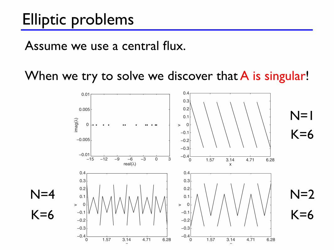
Elliptic problems

Assume we use a central flux.

When we try to solve we discover that A is singular!


subject to u(0) = u(2!) = 0 and with the exact solution u(x) = sin(x). Weuse HeatCRHS1D.m to build the discrete approximation

Auh = fh,

to the second order problem by simply calling HeatCRHS1D.m with the Np!Ksize identity matrix, one unit-vector at a time.

When attempting to invert A, one quickly realizes, however, that the ma-trix is singular. This is in contrast to the continuous problem, which is uniquelysolvable. The question arises of what is causing this sudden breakdown andwhy we did not experience problems when solving the heat equation.

The singularity of the discrete operator indicates that it has at leastone zero eigenvalue – in contrast to the continuous case in which there arenone once the boundary conditions are enforced. To understand the severityof the problem, we show in Fig. 7.6 the computed eigenvalues of A close tothe real axis, confirming that all eigenvalues are negative and real but alsothat there is at least one zero eigenvalue. A closer inspection reveals thatthere is exactly one such zero eigenvalue and in Fig. 7.6 we also show thecorresponding eigenvector, v, for N = 1, 2, 4 and K = 6.

!15 !12 !9 !6 !3 0 3!0.01

!0.005

0

0.005

0.01

real(!)

imag(!)

0 1.57 3.14 4.71 6.28!0.4

!0.3

!0.2

!0.1

0

0.1

0.2

0.3

0.4

x

v

0 1.57 3.14 4.71 6.28!0.4

!0.3

!0.2

!0.1

0

0.1

0.2

0.3

0.4

x

v

0 1.57 3.14 4.71 6.28!0.4

!0.3

!0.2

!0.1

0

0.1

0.2

0.3

0.4

x

v

Fig. 7.6. Top left shows the eigenvalues of the discrete Poisson operator, confirmingthat it is singular. In the remaining three figures is shown the corresponding singulareigenmode for K = 6 and N = 1, N = 2, and N = 4, respectively in a clockwisedirection with N = 1 in the top right corner.

N=1

N=4 N=2

K=6

K=6 K=6

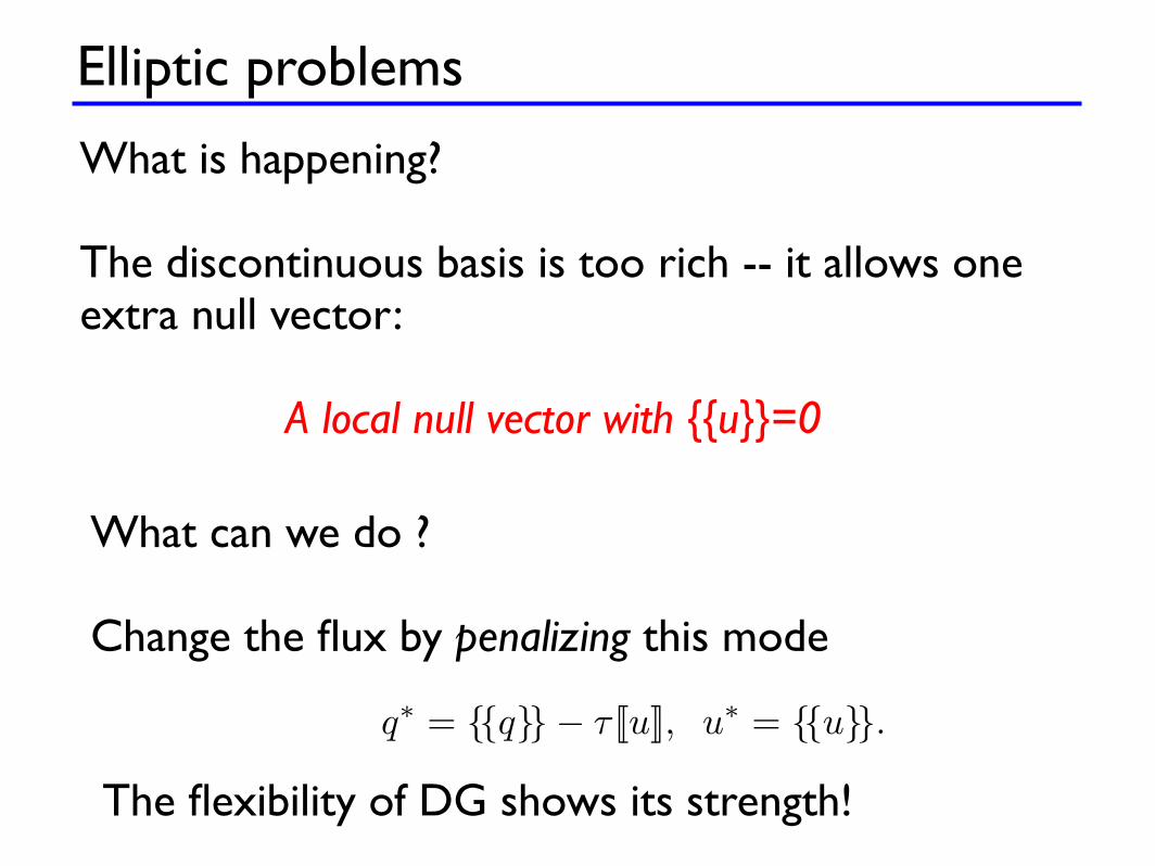
Elliptic problems

What is happening?

The discontinuous basis is too rich -- it allows one extra null vector:

A local null vector with {{u}}=0

What can we do ?

Change the flux by penalizing this mode


The eigenvectors for the three di!erent orders of approximation share somedistinct features. First, we notice that they are all piecewise linear inside theelements, as required to ensure that their second derivative reduces to zero.However, we also note that the eigenvectors v all share the property that

v! = !v+, (7.3)

at any internal interface. Since we are using a central flux, which vanishesexactly for this choice of values, all the elements e!ectively decouple. On theother hand, this condition is the same condition that we use to impose homo-geneous Dirichlet boundary conditions so that at the interfaces it appears as ifwe have the correct zero solution. It is the added freedom in the discontinuousbasis that comes back to bite us by allowing too much flexibility, which wecannot control using the simple central flux.

This also explains why this particular spurious mode caused no problemsin the time-dependent problem as it is characterized by being constant in timeand very rapidly varying in space. As long as the solutions are well resolved,this mode will not cause any problems. However, for marginally resolved prob-lems, the situation may be a little more delicate and the spurious mode mayimpact the accuracy. In such cases, the stabilization methods developed forthe elliptic case can also be useful to improve the accuracy for time-dependentproblems.

With this added understanding, we can ask ourselves what to do aboutit. An obvious solution would be, at least asymptotically in N and/or h,to disallow the eigenmode with the properties in Eq. (7.3) without it alsovanishing inside the element; that is, to remove the artificial null-space.

The discontinuous Galerkin (DG) method now shows one of its strengthsby allowing us to modify the choice of the numerical flux. In particular, letus consider a set of numerical fluxes as

q" = {{q}}! ! [[u]], u" = {{u}}.

For ! = 0 this reduces to the central flux. The role of the added term is topenalize the solution to disallow large jumps in u; clearly if we introduce oneof the null vectors with the property in Eq. (7.3), the added penalty termwould highlight the jump. The parameter ! is chosen to control this jump.

The minor change of the flux required is illustrated in HeatCstabRHS1D.m,which should be compared with HeatCRHS1D.m discussed Section 7.1. Indeed,as expected, taking ! > 0 makes A, the discrete approximation to the Poissonequation, invertible by pushing the zero eigenmode out of the kernel.

HeatCstabRHS1D.m

function [rhsu] = HeatCstabRHS1D(u,time)

% function [rhsu] = HeatCstabRHS1D(u,time)% Purpose : Evaluate RHS flux in 1D heat equation using stabilized% central flux

The flexibility of DG shows its strength!

Elliptic problems

Does it work?


Let us consider a simple example to illustrate the performance whensolving the one-dimensional Poisson equation.

Example 7.7. Consider the problem

d2u

dx2= ! sin(x), x " [0, 2!],

with u(0) = u(2!) = 0.The routine for setting up the discrete Poisson operator is shown in Pois-

sonCstabRHS1D.m, and in PoissonCstabDriver1D.m, we illustrate the driverroutine needed to solve the problem.

PoissonCstab1D.m

function [A] = PoissonCstab1D();

% function [A] = PoissonCstab1D();% Purpose: Set up symmetric Poisson matrix with estabilized% central fluxes

Globals1D;A = zeros(K*Np); g = zeros(K*Np,1);

% Build matrix -- one column at a timefor i=1:K*Np

g(i) = 1.0;gmat = reshape(g,Np,K);Avec = PoissonCstabRHS1D(gmat);A(:,i) = reshape(Avec,K*Np,1);g(i)=0.0;

endreturn

PoissonCDriver1D.m

% Driver script for solving the 1D Poisson equationGlobals1D;

% Polynomial order used for approximationN =4;

% Read in Mesh[Nv, VX, K, EToV] = MeshGen1D(0,2*pi,10);

% Initialize solver and construct grid and metricStartUp1D;


Let us consider a simple example to illustrate the performance whensolving the one-dimensional Poisson equation.

Example 7.7. Consider the problem

d2u

dx2= ! sin(x), x " [0, 2!],

with u(0) = u(2!) = 0.The routine for setting up the discrete Poisson operator is shown in Pois-

sonCstabRHS1D.m, and in PoissonCstabDriver1D.m, we illustrate the driverroutine needed to solve the problem.

PoissonCstab1D.m

function [A] = PoissonCstab1D();

% function [A] = PoissonCstab1D();% Purpose: Set up symmetric Poisson matrix with estabilized% central fluxes

Globals1D;A = zeros(K*Np); g = zeros(K*Np,1);

% Build matrix -- one column at a timefor i=1:K*Np

g(i) = 1.0;gmat = reshape(g,Np,K);Avec = PoissonCstabRHS1D(gmat);A(:,i) = reshape(Avec,K*Np,1);g(i)=0.0;

endreturn

PoissonCDriver1D.m

% Driver script for solving the 1D Poisson equationGlobals1D;

% Polynomial order used for approximationN =4;

% Read in Mesh[Nv, VX, K, EToV] = MeshGen1D(0,2*pi,10);

% Initialize solver and construct grid and metricStartUp1D;


% Set RHSf = -J.*((invV’*invV)*sin(x));

% Set up operator[A] = PoissonCstab1D();

% Solve Problemsolvec = A\f(:);u = reshape(solvec,Np,K);

101 10210!12

10!10

10!8

10!6

10!4

10!2

100

K ! 1/h

|| u !

uh ||

N=1

N=2

N=3

N=4

h2

h3

h4

h5

0 20 40 60 80

0

10

20

30

40

50

60

70

80

nz = 622

Fig. 7.7. On the left, we show the convergence rate for the solving the homogeneousPoisson problem with a stabilized central flux. On the right is shown the sparsitypattern for K = 20 and N = 3 of the discrete Poisson operator based on this flux.

The problem is solved with di!erent number of elements and orders ofapproximation, and we show the results in Fig. 7.7, obtained with ! = 1 forthe stabilization parameter. The results indicate optimal rates of convergence,O(hN+1).

One can naturally question whether the LDG flux, introduced to recoveroptimal convergence in Section 7.1 for the heat equation, can also be used todiscretize the Poisson problem. This is naturally possible and we show in Fig.7.8 the results of solving the problem in Example 7.5 using a local stabilizedflux of the kind

q!h = {{qh}} + ! · [[qh]] ! ! [[uh]], u!h = {{uh}}! ! · [[uh]],

with ! = 1 for all cases and ! = ±n. As in Fig. 7.7, we recover an optimalconvergence rate. The code used to solve the problem is a direct combinationof PoissonCstabRHS1D.m and HeatLDGRHS1D.m.

If we now compare the two plots of the nonzero elements in Fig. 7.7 andFig. 7.8, we note that the latter, based on the LDG fluxes, is considerablysparser that the former, based on the central fluxes.

What about the other flux - the LDG flux?

Elliptic problems

Consider the stabilized LDG flux


101 10210!12

10!10

10!8

10!6

10!4

10!2

100

K ! 1/h

|| u !

uh

||

N=1

N=2

N=3

N=4

h2

h3

h4

h5

0 20 40 60 80

0

10

20

30

40

50

60

70

80

nz = 472

Fig. 7.8. On the left, we show the convergence rate for the solving the homogeneousPoisson problem with a stabilized LDG flux. On the right is shown the sparsitypattern of the discrete Poisson operator based on this flux.

To appreciate the source of this, consider the simplest schemes with N = 0.In this case the scheme for element k becomes

q!h(qkh, qk+1

h , ukh, uk+1

h ) ! q!h(qkh, qk"1

h , ukh, uk"1

h ) = hfkh ,

u!h(uk

h, uk+1h ) ! u!

h(ukh, uk"1

h ) = hgkh.

If we first consider the central flux with

q!h(q"h , q+h , u"

h , u+h ) = {{qh}}! ! [[uh]], u!

h(u"h , u+

h ) = {{uh}},

we recoveruk+2

h ! 2ukh + uk"2

h

(2h)2+ !

uk+1h ! uk"1

h

h= fk

h . (7.4)

One notices that the stencil is wider than would be expected; that is, thestandard second-order finite di!erence method uses only the nearest neighborsin contrast to the central stencil in Eq. (7.4), which engages two levels ofelements.

If we instead consider the LDG flux

q!h(q"h , q+h , u"

h , u+h ) = q"h ! ! [[uh]], u!

h(u"h , u+

h ) = u+h ,

we recover the stencil

uk+1h ! 2uk

h + uk"1h

h2+ !

uk+1h ! uk"1

h

h= fk

h . (7.5)

This leads to a more compact stencil by relying only on the nearest neighbors.The sparsity patterns in Figs. 7.7 and 7.8 reflect how this carries over to thegeneral high-order case where the choice of the LDG flux generally leads toa much sparser operator. The extension to the multidimensional case is less

Works fine as expected - but we also notethat A is much more sparse!

Elliptic problems

Why is one more sparse than the other?

Consider the N=0 case


101 10210!12

10!10

10!8

10!6

10!4

10!2

100

K ! 1/h

|| u !

uh

||

N=1

N=2

N=3

N=4

h2

h3

h4

h5

0 20 40 60 80

0

10

20

30

40

50

60

70

80

nz = 472



q!h(qkh, qk+1

h , ukh, uk+1

h ) ! q!h(qkh, qk"1

h , ukh, uk"1

h ) = hfkh ,

u!h(uk

h, uk+1h ) ! u!

h(ukh, uk"1

h ) = hgkh.


q!h(q"h , q+h , u"

h , u+h ) = {{qh}}! ! [[uh]], u!

h(u"h , u+

h ) = {{uh}},

we recoveruk+2

h ! 2ukh + uk"2

h

(2h)2+ !

uk+1h ! uk"1

h

h= fk

h . (7.4)



q!h(q"h , q+h , u"

h , u+h ) = q"h ! ! [[uh]], u!

h(u"h , u+

h ) = u+h ,


uk+1h ! 2uk

h + uk"1h

h2+ !

uk+1h ! uk"1

h

h= fk

h . (7.5)



101 10210!12

10!10

10!8

10!6

10!4

10!2

100

K ! 1/h

|| u !

uh

||

N=1

N=2

N=3

N=4

h2

h3

h4

h5

0 20 40 60 80

0

10

20

30

40

50

60

70

80

nz = 472



q!h(qkh, qk+1

h , ukh, uk+1

h ) ! q!h(qkh, qk"1

h , ukh, uk"1

h ) = hfkh ,

u!h(uk

h, uk+1h ) ! u!

h(ukh, uk"1

h ) = hgkh.


q!h(q"h , q+h , u"

h , u+h ) = {{qh}}! ! [[uh]], u!

h(u"h , u+

h ) = {{uh}},

we recoveruk+2

h ! 2ukh + uk"2

h

(2h)2+ !

uk+1h ! uk"1

h

h= fk

h . (7.4)



q!h(q"h , q+h , u"

h , u+h ) = q"h ! ! [[uh]], u!

h(u"h , u+

h ) = u+h ,


uk+1h ! 2uk

h + uk"1h

h2+ !

uk+1h ! uk"1

h

h= fk

h . (7.5)



101 10210!12

10!10

10!8

10!6

10!4

10!2

100

K ! 1/h

|| u !

uh

||

N=1

N=2

N=3

N=4

h2

h3

h4

h5

0 20 40 60 80

0

10

20

30

40

50

60

70

80

nz = 472



q!h(qkh, qk+1

h , ukh, uk+1

h ) ! q!h(qkh, qk"1

h , ukh, uk"1

h ) = hfkh ,

u!h(uk

h, uk+1h ) ! u!

h(ukh, uk"1

h ) = hgkh.


q!h(q"h , q+h , u"

h , u+h ) = {{qh}}! ! [[uh]], u!

h(u"h , u+

h ) = {{uh}},

we recoveruk+2

h ! 2ukh + uk"2

h

(2h)2+ !

uk+1h ! uk"1

h

h= fk

h . (7.4)



q!h(q"h , q+h , u"

h , u+h ) = q"h ! ! [[uh]], u!

h(u"h , u+

h ) = u+h ,


uk+1h ! 2uk

h + uk"1h

h2+ !

uk+1h ! uk"1

h

h= fk

h . (7.5)



101 10210!12

10!10

10!8

10!6

10!4

10!2

100

K ! 1/h

|| u !

uh

||

N=1

N=2

N=3

N=4

h2

h3

h4

h5

0 20 40 60 80

0

10

20

30

40

50

60

70

80

nz = 472



q!h(qkh, qk+1

h , ukh, uk+1

h ) ! q!h(qkh, qk"1

h , ukh, uk"1

h ) = hfkh ,

u!h(uk

h, uk+1h ) ! u!

h(ukh, uk"1

h ) = hgkh.


q!h(q"h , q+h , u"

h , u+h ) = {{qh}}! ! [[uh]], u!

h(u"h , u+

h ) = {{uh}},

we recoveruk+2

h ! 2ukh + uk"2

h

(2h)2+ !

uk+1h ! uk"1

h

h= fk

h . (7.4)



q!h(q"h , q+h , u"

h , u+h ) = q"h ! ! [[uh]], u!

h(u"h , u+

h ) = u+h ,


uk+1h ! 2uk

h + uk"1h

h2+ !

uk+1h ! uk"1

h

h= fk

h . (7.5)



101 10210!12

10!10

10!8

10!6

10!4

10!2

100

K ! 1/h

|| u !

uh

||

N=1

N=2

N=3

N=4

h2

h3

h4

h5

0 20 40 60 80

0

10

20

30

40

50

60

70

80

nz = 472



q!h(qkh, qk+1

h , ukh, uk+1

h ) ! q!h(qkh, qk"1

h , ukh, uk"1

h ) = hfkh ,

u!h(uk

h, uk+1h ) ! u!

h(ukh, uk"1

h ) = hgkh.


q!h(q"h , q+h , u"

h , u+h ) = {{qh}}! ! [[uh]], u!

h(u"h , u+

h ) = {{uh}},

we recoveruk+2

h ! 2ukh + uk"2

h

(2h)2+ !

uk+1h ! uk"1

h

h= fk

h . (7.4)



q!h(q"h , q+h , u"

h , u+h ) = q"h ! ! [[uh]], u!

h(u"h , u+

h ) = u+h ,


uk+1h ! 2uk

h + uk"1h

h2+ !

uk+1h ! uk"1

h

h= fk

h . (7.5)


Using the central flux yields

Using the LDG flux yields

Wide

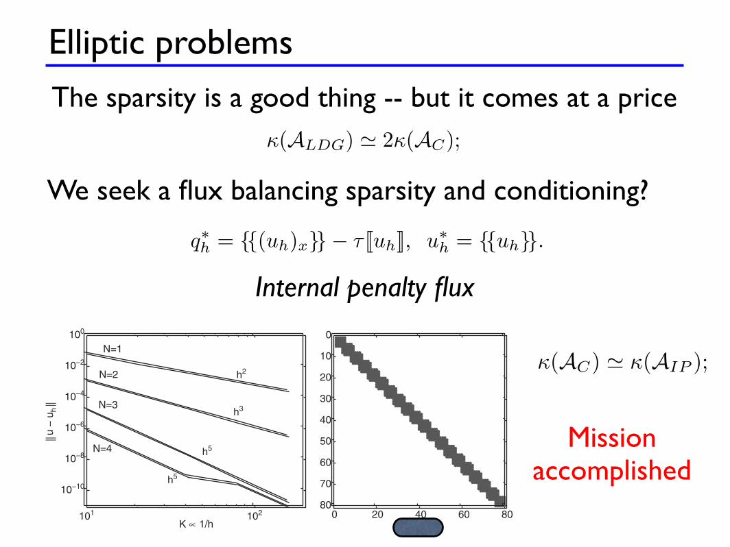
Elliptic problems

The sparsity is a good thing -- but it comes at a price


dramatic in terms of sparsity as LDG no longer guarantees nearest neigh-bor connections on general grids, although it will remain sparser than themultidimensional version of the central fluxes [252, 283].

The more compact discrete operator/stencil does, however, come at a price.If we compute the condition number, !, one observes that

!(ALDG) ! 2!(AC);

that is, the condition number of the LDG-based discrete operators is abouttwice that of the operator based on central fluxes. The impact of this is aslightly worse accuracy of direct solvers and increased iteration counts whenan iterative solver is used to solve the linear system.

Trying to balance sparsity and the conditioning, a possible compromise isthe internal penalty flux, defined as

q!h = {{(uh)x}}" " [[uh]], u!h = {{uh}}.

We note that for N = 0, the flux q!h depends solely on the penalty term. Thisindicates, as we will discuss shortly, that the value of " plays a larger role forthe internal penalty flux than for the previous two cases.

Nevertheless, to first convince ourselves that this approach works, we re-peat the problem in Example 7.5 using the internal penalty flux, and we showthe results in Fig. 7.9. As one could hope, we observe optimal rates of con-vergence and, when comparing with Figs. 7.7 and 7.8, a sparsity pattern inthe discrete operator in between those obtained with the central flux and theLDG flux. Furthermore, the condition number behaves as

!(AC) ! !(AIP );

that is, the internal penalty method appears to o!er a suitable compromisebetween central fluxes and LDG fluxes. An example of the implementation ofinternal penalty flux is shown in PoissonIPstabRHS1D.m.

101 102

10!10

10!8

10!6

10!4

10!2

100

K ! 1/h

|| u !

uh ||

N=1

N=2

N=3

N=4

h2

h3

h5

h5

0 20 40 60 80

0

10

20

30

40

50

60

70

80

nz = 586

Fig. 7.9. On the left, we show the convergence rate for the solving the homogeneousPoisson problem with a stabilized internal penalty flux. On the right is shown thesparsity pattern of the discrete Poisson operator based on this flux.

We seek a flux balancing sparsity and conditioning?




!(ALDG) ! 2!(AC);



q!h = {{(uh)x}}" " [[uh]], u!h = {{uh}}.



!(AC) ! !(AIP );


101 102

10!10

10!8

10!6

10!4

10!2

100

K ! 1/h

|| u !

uh ||

N=1

N=2

N=3

N=4

h2

h3

h5

h5

0 20 40 60 80

0

10

20

30

40

50

60

70

80

nz = 586


Internal penalty flux




!(ALDG) ! 2!(AC);



q!h = {{(uh)x}}" " [[uh]], u!h = {{uh}}.



!(AC) ! !(AIP );


101 102

10!10

10!8

10!6

10!4

10!2

100

K ! 1/h

|| u !

uh ||

N=1

N=2

N=3

N=4

h2

h3

h5

h5

0 20 40 60 80

0

10

20

30

40

50

60

70

80

nz = 586


Mission accomplished

Elliptic problems

The sparsity is a good thing -- but it comes at a price




!(ALDG) ! 2!(AC);



q!h = {{(uh)x}}" " [[uh]], u!h = {{uh}}.



!(AC) ! !(AIP );


101 102

10!10

10!8

10!6

10!4

10!2

100

K ! 1/h

|| u !

uh ||

N=1

N=2

N=3

N=4

h2

h3

h5

h5

0 20 40 60 80

0

10

20

30

40

50

60

70

80

nz = 586


We seek a flux balancing sparsity and conditioning?




!(ALDG) ! 2!(AC);



q!h = {{(uh)x}}" " [[uh]], u!h = {{uh}}.



!(AC) ! !(AIP );


101 102

10!10

10!8

10!6

10!4

10!2

100

K ! 1/h

|| u !

uh ||

N=1

N=2

N=3

N=4

h2

h3

h5

h5

0 20 40 60 80

0

10

20

30

40

50

60

70

80

nz = 586


Internal penalty flux




!(ALDG) ! 2!(AC);



q!h = {{(uh)x}}" " [[uh]], u!h = {{uh}}.



!(AC) ! !(AIP );


101 102

10!10

10!8

10!6

10!4

10!2

100

K ! 1/h

|| u !

uh ||

N=1

N=2

N=3

N=4

h2

h3

h5

h5

0 20 40 60 80

0

10

20

30

40

50

60

70

80

nz = 586





!(ALDG) ! 2!(AC);



q!h = {{(uh)x}}" " [[uh]], u!h = {{uh}}.



!(AC) ! !(AIP );


101 102

10!10

10!8

10!6

10!4

10!2

100

K ! 1/h

|| u !

uh ||

N=1

N=2

N=3

N=4

h2

h3

h5

h5

0 20 40 60 80

0

10

20

30

40

50

60

70

80

nz = 586


Mission accomplished

Elliptic problems

Remaining question: How do you choose ?!

The analysis shows that:

✓ For the central flux, suffices✓ For the LDG flux, suffices✓ For the IP flux, one must require

! > 0! > 0


Let us now return to the question of how to choose the penalty parame-ter, ! . As we will show rigorously in Section 7.2.2, for schemes based on centralor LDG fluxes, it su!ces to take ! > 0 to ensure invertibility and a purelynegative real spectrum [13, 48, 49]. However, for the internal penalty-basedscheme, we must require that

! ! C(N + 1)2

h, C ! 1,

to guarantee similar properties. The bound on C is derived in [281].Whereas these results ensure invertibility and definiteness, the actual value

of ! may well a"ect both the conditioning and the accuracy of the scheme. Infact, as we will see, the actual value of ! has quite a di"erent impact on theschemes.

PoissonIPstabRHS1D.m

function [rhsu] = PoissonIPstabRHS1D(u)

% function [rhsu] = PoissonIPstabRHS1D(u)% Purpose : Evaluate RHS in 1D Poisson equation on symmetric form% using stabilized internal penalty flux

Globals1D;

% Define field differences at facesdu = zeros(Nfp*Nfaces,K); du(:) = u(vmapM)-u(vmapP);

% impose boundary condition -- Dirichlet BC’suin = -u(vmapI); du(mapI) = u(vmapI)-uin;uout = -u(vmapO); du(mapO) = u(vmapO)-uout;

% Compute qfluxu = nx.*du/2.0;ux = rx.*(Dr*u);q = ux - LIFT*(Fscale.*fluxu);dq = zeros(Nfp*Nfaces,K);dq(:) = q(vmapM)-(ux(vmapM)+ux(vmapP))/2.0;

% impose boundary condition -- Neumann BC’sqin = ux(vmapI); dq (mapI) = q(vmapI) - (ux(vmapI)+ qin )/2.0;qout = ux(vmapO); dq (mapO) = q(vmapO) - (ux(vmapO)+ qout)/2.0;

% evaluate fluxeshmin = 2.0/max(max(rx)); tau = Np^2/hmin;fluxq = nx.*(dq+tau*nx.*du);

% compute right hand sides of the semi-discrete PDErhsu = J.*((invV’*invV)*(rx.*(Dr*q) - LIFT*(Fscale.*fluxq)));return

These suffices to guarantee stability, but they may not give the best accuracy

Generally, a good choice is


Let us now return to the question of how to choose the penalty parame-ter, ! . As we will show rigorously in Section 7.2.2, for schemes based on centralor LDG fluxes, it su!ces to take ! > 0 to ensure invertibility and a purelynegative real spectrum [13, 48, 49]. However, for the internal penalty-basedscheme, we must require that

! ! C(N + 1)2

h, C ! 1,

to guarantee similar properties. The bound on C is derived in [281].Whereas these results ensure invertibility and definiteness, the actual value

of ! may well a"ect both the conditioning and the accuracy of the scheme. Infact, as we will see, the actual value of ! has quite a di"erent impact on theschemes.

PoissonIPstabRHS1D.m

function [rhsu] = PoissonIPstabRHS1D(u)

% function [rhsu] = PoissonIPstabRHS1D(u)% Purpose : Evaluate RHS in 1D Poisson equation on symmetric form% using stabilized internal penalty flux

Globals1D;

% Define field differences at facesdu = zeros(Nfp*Nfaces,K); du(:) = u(vmapM)-u(vmapP);

% impose boundary condition -- Dirichlet BC’suin = -u(vmapI); du(mapI) = u(vmapI)-uin;uout = -u(vmapO); du(mapO) = u(vmapO)-uout;

% Compute qfluxu = nx.*du/2.0;ux = rx.*(Dr*u);q = ux - LIFT*(Fscale.*fluxu);dq = zeros(Nfp*Nfaces,K);dq(:) = q(vmapM)-(ux(vmapM)+ux(vmapP))/2.0;

% impose boundary condition -- Neumann BC’sqin = ux(vmapI); dq (mapI) = q(vmapI) - (ux(vmapI)+ qin )/2.0;qout = ux(vmapO); dq (mapO) = q(vmapO) - (ux(vmapO)+ qout)/2.0;

% evaluate fluxeshmin = 2.0/max(max(rx)); tau = Np^2/hmin;fluxq = nx.*(dq+tau*nx.*du);

% compute right hand sides of the semi-discrete PDErhsu = J.*((invV’*invV)*(rx.*(Dr*q) - LIFT*(Fscale.*fluxq)));return

Elliptic problems

What can we say more generally?

Consider


37 % set up boundary condition38 ubc = zeros(gauss.NGauss*Nfaces*K,1);39 xbc = gauss.x(gauss.mapD); ybc = gauss.y(gauss.mapD);40 ubc(gauss.mapD) = sin(pi*xbc).*sin(pi*ybc);41 xbc = gauss.x(gauss.mapN); ybc = gauss.y(gauss.mapN);42 ubc(gauss.mapN) = ...43 gauss.nx(gauss.mapN).*(pi*cos(pi*xbc).*sin(pi*ybc)) + ...44 gauss.ny(gauss.mapN).*(pi*sin(pi*xbc).*cos(pi*ybc));45

46 ubc = Abc*ubc;47

48 % solve linear system49 solvec = (A+M)\(M*(-f(:)) + ubc);50 u = reshape(solvec, Np, K);

In this particular example, we take a minor liberty with the evaluation ofthe right-hand-side portion of the load vector by interpolating f at the ele-mental Lagrange interpolation nodes and then evaluating the inner products.Alternatively, one can evaluate f at cubature nodes in each element and thenevaluate the inner products accordingly.

7.2.2 A look at basic theoretical properties

To gain a better understanding of the behavior we have observed in the lastsections, let us develop some of the basic theory for DG approximations ofelliptic problems.

To keep things simple, we primarily discuss the di!erent schemes in thecontext of Poisson’s equation but conclude with a few remarks and referencesfor more general problems.

Recall the Poisson equation

!"2u(x) = f(x), x # !,

subject to homogeneous Dirichlet boundary conditions as

u(x) = 0, x # "!.

Existence and uniqueness of solutions to this problem is well understood [59]under light conditions on f and !. The variational formulation for findingu # H1

0 (!) is

a(u,#) =!

!"u ·"# dx = (f, v)! , $# # H1

0 (!).

Here, H10 (!) is the space of functions u # H1(!) for which u = 0 on "!.

This is the essential statement of coercivity.


Table 7.3. Overview of numerical flux choices

u!h q!

h

Central flux {{uh}} {{qh}}! ! [[uh]]Local DG flux (LDG) {{uh}} + ! · [[uh]] {{qh}}! ![[qh]] ! ! [[uh]]Internal penalty flux (IP) {{uh}} {{"uh}}! ! [[uh]]

We follow the approach outlined previously and rewrite the problem as afirst-order system

!" · q = f, q = "u. (7.7)Let us now seek polynomial solutions, uh # Vh = $K

k=1PN (Dk), where werecall that PN (Dk) is the space of N -th-order polynomials defined on Dk andqh # Uh = Vh % Vh := V2

h. Following the standard DG approach, we seek(uh, qh) for all test functions (!h,"h) # Vh % Uh such that

(qh,"!h)!,h !K!

k=1

(n · q!h,!h)"Dk = (f,!h)!,h , (7.8)

(qh,"h)!,h =K!

k=1

(u!h, n · "h)"Dk ! (uh," · "h)!,h . (7.9)

We have introduced the numerical flux pair (u!h, q!

h) to connect elements andwe summarize in Table 7.3 the choices discussed previously. Recall the stan-dard notation that

{{u}} =u" + u+

2,

where u can be both a scalar or a vector. Similarly, we define the jumps alonga normal, n, in the standard notation as

[[u]] = n"u" + n+u+, [[u]] = n" · u" + n+ · u+.

We note that there are several lesser used alternatives to these three optionsfor the numerical fluxes and we refer to [13] for a complete discussion of these.

Primal forms and consistency

To get a better understanding of the di!erent schemes, let us eliminate theauxiliary variable, qh, to recover the primal form of the discretization. Toachieve this we need the following result:

Lemma 7.9. Assume that " has been triangulated into K elements, Dk. ThenK!

k=1

(n · u, v)"Dk ="

"{{u}} · [[v]] dx +

"

"i

{{v}}[[u]] dx,

where # represents the set of unique edges and #i the set of unique purelyinternal edges.



u!h q!

h






(qh,"!h)!,h !K!

k=1

(n · q!h,!h)"Dk = (f,!h)!,h , (7.8)

(qh,"h)!,h =K!

k=1

(u!h, n · "h)"Dk ! (uh," · "h)!,h . (7.9)



{{u}} =u" + u+

2,


[[u]] = n"u" + n+u+, [[u]] = n" · u" + n+ · u+.





k=1

(n · u, v)"Dk ="

"{{u}} · [[v]] dx +

"

"i

{{v}}[[u]] dx,




u!h q!

h






(qh,"!h)!,h !K!

k=1

(n · q!h,!h)"Dk = (f,!h)!,h , (7.8)

(qh,"h)!,h =K!

k=1

(u!h, n · "h)"Dk ! (uh," · "h)!,h . (7.9)



{{u}} =u" + u+

2,


[[u]] = n"u" + n+u+, [[u]] = n" · u" + n+ · u+.





k=1

(n · u, v)"Dk ="

"{{u}} · [[v]] dx +

"

"i

{{v}}[[u]] dx,


Discretized as

Using one of the fluxes

Elliptic problems

For the 3 discrete systems, one can prove (see text)

✓ They are all symmetric for any N✓ The are all invertible provided stabilization is used✓ The discretization is consistent✓ The adjoint problem is consistent✓ They have optimal convergence in L2

Many of these results can be extended to more general problems (saddle-point, non-coercive etc)

There are other less used fluxes also

Solving the systems

After things are discretized, we end up with

7.3 Intermission of solving linear systems 297

systems are banded, making a direct solver the natural choice. However, forthe multidimensional case, the situation is more complex, as the linear systemsare sparse but with a structure that depends on the grid connectivity.

This is not intended to be a comprehensive review, but rather a study ofsolver technology conveniently made available through Matlab. Further infor-mation be found in some of the many excellent texts on computational linearalgebra [104, 141, 275, 308]. We will include some comments on our experi-ence of their positive and negative aspects. At this time, it is unclear whichapproach is best for general DG discretizations and we demur on some moreaggressive strategies such as the algebraic multigrid [119, 150, 245] and do-main decomposition-based multilevel solvers [117, 133, 193, 213]. In addition,we mostly discuss techniques that are suitable for solving the same linear sys-tems with multiple di!erent right-hand sides, as one might encounter whenimplicitly timestepping partial di!erential equations.

As an example for experimentation, we consider the linear Poisson equa-tion

!2u = f(x, y) =!!

16 " n2"r2 +

!n2 " 36

"r4

"sin (n!), x2 + y2 # 1,

where n = 12, r =#

x2 + y2, ! = arctan (y, x) and the exact solution, u(x, y)is imposed at the boundary of ".

Using a DG formulation with internal penalty fluxes and K = 512 ele-ments, each of fourth order, we have a total of 7680 degrees of freedom. Tocompute these, we need to solve Auh = fh for the solution vector u. The dis-crete operator A, is a square matrix with a total of 284,100 nonzero entries,reflecting a sparsity exceeding 95%.

7.3.1 Direct methods

We first consider the use of an LU-factorization of the matrix such that A =LU , where the factor matrices are logically lower and upper triangular to allowtheir e"cient inversion. In Matlab the factorization and solution is achievedwith

>> [L, U] = lu(A);

>> u = U\(L\f);

This requires storage for the sparse matrices (A,L,U) which, in our test case,required storage for 8,149,974 extra nonzeros in (L,U). It is evident that thesparsity pattern of A is not compactly represented near the diagonal, so theLU-factorization process creates factor matrices with significantly fill in; thatis, significantly more storage is required for L and U than for A. For smallerproblems, this is less of a problem, but as problems increase in size this growthin memory usage becomes a significant concern.

We can solve this in two different ways

✓ Direct methods

✓ Iterative methods

The ‘right’ choice depends on things such as size, speed, sparsity etc

Solving the systems

Direct methods are ‘LU’ based





!2u = f(x, y) =!!

16 " n2"r2 +

!n2 " 36

"r4

"sin (n!), x2 + y2 # 1,

where n = 12, r =#





>> [L, U] = lu(A);

>> u = U\(L\f);


Example:





!2u = f(x, y) =!!

16 " n2"r2 +

!n2 " 36

"r4

"sin (n!), x2 + y2 # 1,

where n = 12, r =#





>> [L, U] = lu(A);

>> u = U\(L\f);






!2u = f(x, y) =!!

16 " n2"r2 +

!n2 " 36

"r4

"sin (n!), x2 + y2 # 1,

where n = 12, r =#





>> [L, U] = lu(A);

>> u = U\(L\f);


K=512N=4

7680 DoF

Solving the systems298 7 Higher-order equations

Fig. 7.14. On the left, we show the sparsity pattern of the discrete Poisson matrixbefore reverse Cuthill-McKee reordering. On the right, we show the sparsity patternafter the reordering.

To reduce the amount of fill in for the LU-factors, one can explore re-ordering of the degrees of freedom to minimize the bandwidth of the matrixas much a possible. A powerful approach for this is the reverse Cuthill-McKeenumbering system [125]. This is a built-in method in Matlab and provides apermutation vector for a given sparse symmetric matrix to significantly reducethe distance of any nonzero entry from the diagonal. To illustrate the e!ectof this reordering, we contrast in Fig. 7.14 the sparsity patterns of A beforeand after reordering.

To take advantage of this in the solution of the linear system, one can usethe following approach in which a permutation vector is computed, appliedto the row and column swaps to A, permute f , solve the two systems, andpermute the solution:

>> P = symrcm(A);>> A = A(P,P);>> rhs = rhs(P);>> [L,U] = lu(A);>> u = U\(L\f);>> u(P) = u;

This simple procedure reduces the number of nonzeros in the LU-factors to3,802,198 (i.e., a reduction of more than 50%). All subsequent tests use thereordered A matrix.

We can further reduce the storage requirements by taking advantage of Abeing a positive definite symmetric matrix and use a Cholesky factorization;that is, find the matrix C such that A = CTC using

Reordering is needed !

8,7m extra non-zero entries in (L,U)

Cuthill-McKee ordering

3,7m extra non-zero entries in (L,U)

Solving the systems

Re-ordering:







We can further reduce the storage requirements by taking advantage of Abeing a positive definite symmetric matrix and use a Cholesky factorization;that is, find the matrix C such that A = CTC using

.. but A is SPD:







We can further reduce the storage requirements by taking advantage of Abeing a positive definite symmetric matrix and use a Cholesky factorization;that is, find the matrix C such that A = CTC usingCholesky decomp7.3 Intermission of solving linear systems 299

>> C = chol(A);>> u = C\(C’\f);

In combination with the reordering, the number of extra nonzeros is reducedto 1,901,109.

7.3.2 Iterative methods

For the direct methods discussed above, it is evident that the additional stor-age requirement for the factors may become excessive. With this in mind, it isreasonable to consider Krylov subspace iterative methods as a suitable alter-native. Because matrix A is symmetric positive-definite, we use the conjugategradient (CG) method to solve the system to a chosen tolerance. Again, wecan use Matlab’s suite of iterative solvers to our advantage, allowing a solutionto be obtained by:

>> ittol = 1e-8; maxit = 1000;>> u = pcg(A, f, ittol, maxit);

This solves the system using the CG method. There are no significant extrastorage requirements beyond the system matrix A and f , which is a definiteadvantage. However, one also observes that it takes more than 100 timeslonger to finish the required 818 iterations than when using the reorderedLU-factorization. In the iterative approach, each iteration involves one matrix-vector between A and a residual vector along with a several less expensiveoperations. Clearly, storage is traded for additional execution time.

We can seek to reduce the amount of solver time taken for the conjugategradient solver by choosing to solve

C!1Auh = C!1fh,

where we require that C!1v is easily evaluated for a given vector v and that thepreconditioner, C, approximates A well. A straightforward way to form such apreconditioner is to compute the Cholesky factorization of A but drop entriesthat do not appear in the original sparse pattern of A. Such an incompleteCholesky factorization and its use with the CG methods can be accomplishedin Matlab through

>> ittol = 1e-8; maxit = 1000;>> Cinc = cholinc(OP, ’0’)>> u = pcg(A, f, ittol, maxit, Cinc’, Cinc);

For our sample system, the zero-fill incomplete Cholesky factor requires thestorage of 154,082 entries, but the timing is improved by about a factor of2 (i.e., it remains about 50 times slower than the reordered LU-factorizationmethod). However, notably the number of iterations is reduced to 138 from818 when compared to the nonpreconditioned case.

1,9m extra non-zero entries in C

Solving the systems

If the problem is too large, iterative methods are the only choice


>> C = chol(A);>> u = C\(C’\f);







C!1Auh = C!1fh,




Example requires 818 iterations - 100 times slower than LU !

Solution: Preconditioning


>> C = chol(A);>> u = C\(C’\f);







C!1Auh = C!1fh,




Solving the systems

How to choose the preconditioning ?

.. more an art than a science !

Example - Incomplete Cholesky Preconditioning


>> C = chol(A);>> u = C\(C’\f);







C!1Auh = C!1fh,




Sparsity preserving

138 iterations - but still 50 times slower


We finally supply a finite cut-o! tolerance to the incomplete factorizationthat limits the minimum of the entries that are added to the sparsity patternof the factor. Using a tolerance of 10!4 as in the following:

>> ittol = 1e-8; maxit = 1000; droptol = 1e-4;>> Cinc = cholinc(A, droptol);>> u = pcg(A, b, ittol, maxit, Cinc’, Cinc);

reduces the number of iterations to 17 and yields a dramatic reduction inthe execution time to just four times that of the direct solver. The amountof extra storage increases to 197,927. This again highlights the ability to bal-ance storage and performance by considering di!erent solution techniques andpreconditioners.

It is important to appreciate that these results are specific to the problembeing considered. Generally, one should consider iterative problems for largesparse problems for which excessive memory requirements would otherwisebe a bottleneck. A distinct problem for the straightforward use of iterativemethods is their inability to work with many right-hand sides at the same time.This is in contrast to direct solvers where the reordering and factorization isindependent of the right-hand side. For further discussion and many moredetails on these issues, we refer to [104, 141, 308, 275] and references therein.

7.4 The incompressible Navier-Stokes equations

The dynamics of an incompressible fluid flow in two spatial dimensions isdescribed by the Navier-Stokes equations as

!u

!t+ (u ·!) u = "!p + "!2u, x # #,

! · u = 0,

where u = (u, v), and p are the x-component of the velocity, the y-componentof the velocity, and the scalar pressure field, respectively. In conservative fluxform, the equations are

!u

!t+ ! ·F = "!p + "!2u,

! · u = 0,

with the flux F being

F = [F 1,F 2] =!

u2 uvuv v2

".

The equations are closed with initial conditions on the velocity fields andboundary conditions. In particular, we shall assign di!erent parts of theboundary according to specific boundary conditions; for example, as inflow

Drop tolerance

17 iterations - only 2 times slower

Solving the systems

Choosing fast and efficient linear solvers is not easy -- but there are many options

✓ Direct solvers✓MUMPS (multi-frontal parallel solver)✓SuperLU (fast parallel direct solver)

✓ Iterative solvers✓ Trilinos (large solver/precon library)✓PETSc (large solver/precon library)

Very often you have to try several options and combinations to find the most efficient and robust one(s)

A few examples

So far we have seen lots of theory and “homework” problems.

To see that it also works for more complex problems - but still 2D - let us look at a few examples

✓Incompressible Navier-Stokes✓Boussinesq problems✓Compressible Euler equations

Incompressible fluid flow

Time-dependent Navier-Stokes equations

Written on conservation form

• Water• Low speed• Bioflows• etc

7.4 The incompressible Navier-Stokes equations 279


For our sample system, the zero-fill incomplete Cholesky factor requires the storage of 154,082entries, but the timing is improved by about a factor of 2 (i.e., it remains about 50 times slowerthan the reordered LU-factorization method). However, notably the number of iterations is reducedto 138 from 818 when compared to the nonpreconditioned case.

We finally supply a finite cut-o! tolerance to the incomplete factorization that limits the mini-mum of the entries that are added to the sparsity pattern of the factor. Using a tolerance of 10!4

as in the following:


reduces the number of iterations to 17 and yields a dramatic reduction in the execution time tojust four times that of the direct solver. The amount of extra storage increases to 197,927. Thisagain highlights the ability to balance storage and performance by considering di!erent solutiontechniques and preconditioners.

It is important to appreciate that these results are specific to the problem being considered.Generally, one should consider iterative problems for large sparse problems for which excessivememory requirements would otherwise be a bottleneck. A distinct problem for the straightforwarduse of iterative methods is their inability to work with many right-hand sides at the same time. Thisis in contrast to direct solvers where the reordering and factorization is independent of the right-handside. For further discussion and many more details on these issues, we refer to [104, 141, 308, 275]and references therein.


The dynamics of an incompressible fluid flow in two spatial dimensions is described by the Navier-Stokes equations as

!u

!t+ (u ·!) u = "!p + "!2u, x # #,

! · u = 0,

where u = (u, v), and p are the x-component of the velocity, the y-component of the velocity, andthe scalar pressure field, respectively. In conservative flux form, the equations are

!u

!t+! ·F = "!p + "!2u,

! · u = 0,



F = [F 1,F 2] =!

u2 uvuv v2

".

The equations are closed with initial conditions on the velocity fields and boundary conditions. Inparticular, we shall assign di!erent parts of the boundary according to specific boundary conditions;for example, as inflow !"I , outflow !"O, or walls !"W . The specific boundary conditions appliedon each subset of the boundary will be discussed later.

These equations constitute a mixture of a conservation law, di!usion, and constrained evolution.The mixed nature of these equations makes discrete timestepping a more complicated a!air thanhas been case for the equations we have discussed previously. There are a number of di!erentprocedures mentioned in the literature and we will make no e!ort to provide a thorough overviewof these techniques. Good starting points for such explorations are [97, 198].

7.4.1 Temporal splitting scheme

We consider here the sti"y stable timestepping method [196, 282] in which each timestep breaksinto three stages. The first stage amounts to explicitly integrating the conservation law componentof the equations using an Adams-Bashforth second-order scheme. The second stage involves theprojection of the updated velocity components onto the space of weakly divergence-free functionsand in the final stage, the viscous term is treated implicitly.

First define the nonlinear functions, N (u) = (Nx, Ny) = ! · F , as

Nx (u) = ! · F 1 =!

#u2

$

!x+

! (uv)!y

, Ny (u) = ! · F 2 =! (uv)

!x+

!#v2

$

!y, (7.21)

and express the first part of the timestep as

#0u" $0un " $1un!1

%t= "&0N (un)" &1N (un!1) . (7.22)

This method is second order in time for the velocity (see [143] for details). However, it is not self-starting, in contrast to the Runge-Kutta schemes we have used thus far. For the first timestep wechoose the coe#cients $0,$1,&0,&1 to reduce the scheme to the forward Euler method,

#0 = 0, $0 = 1, $1 = 0, &0 = 1, &1 = 0,

consistent with the assumption that u0 and v0 are provided as initial conditions. The subsequenttimesteps are done with

#0 =32, $0 = 2, $1 = "1

2, &0 = 2, &1 = "1,

reflecting a second-order Adams-Bashforth method.In the second stage, the pressure projection step, the intermediate velocities u are updated using

#0

˜u" u

%t= "!pn+1.

To close this system we seek pn+1 such that the divergence of ˜u is zero by solving for pn+1 as

Solved by stiffly stable time-splitting and pressureprojection

Incompressible fluid flow

Time-dependent Navier-Stokes equations

Written on conservation form

• Water

• Low speed

• Bioflows

• etc











!u

!t+ (u ·!) u = "!p + "!2u, x # #,

! · u = 0,


!u

!t+! ·F = "!p + "!2u,

! · u = 0,












!u

!t+ (u ·!) u = "!p + "!2u, x # #,

! · u = 0,


!u

!t+! ·F = "!p + "!2u,

! · u = 0,



F = [F 1,F 2] =!

u2 uvuv v2

".

The equations are closed with initial conditions on the velocity fields and boundary conditions. Inparticular, we shall assign di!erent parts of the boundary according to specific boundary conditions;for example, as inflow !"I , outflow !"O, or walls !"W . The specific boundary conditions appliedon each subset of the boundary will be discussed later.

These equations constitute a mixture of a conservation law, di!usion, and constrained evolution.The mixed nature of these equations makes discrete timestepping a more complicated a!air thanhas been case for the equations we have discussed previously. There are a number of di!erentprocedures mentioned in the literature and we will make no e!ort to provide a thorough overviewof these techniques. Good starting points for such explorations are [97, 198].


We consider here the sti"y stable timestepping method [196, 282] in which each timestep breaksinto three stages. The first stage amounts to explicitly integrating the conservation law componentof the equations using an Adams-Bashforth second-order scheme. The second stage involves theprojection of the updated velocity components onto the space of weakly divergence-free functionsand in the final stage, the viscous term is treated implicitly.

First define the nonlinear functions, N (u) = (Nx, Ny) = ! · F , as

Nx (u) = ! · F 1 =!

#u2

$

!x+

! (uv)!y

, Ny (u) = ! · F 2 =! (uv)

!x+

!#v2

$

!y, (7.21)


#0u" $0un " $1un!1

%t= "&0N (un)" &1N (un!1) . (7.22)

This method is second order in time for the velocity (see [143] for details). However, it is not self-starting, in contrast to the Runge-Kutta schemes we have used thus far. For the first timestep wechoose the coe#cients $0,$1,&0,&1 to reduce the scheme to the forward Euler method,

#0 = 0, $0 = 1, $1 = 0, &0 = 1, &1 = 0,

consistent with the assumption that u0 and v0 are provided as initial conditions. The subsequenttimesteps are done with

#0 =32, $0 = 2, $1 = "1

2, &0 = 2, &1 = "1,

reflecting a second-order Adams-Bashforth method.In the second stage, the pressure projection step, the intermediate velocities u are updated using

#0

˜u" u

%t= "!pn+1.

To close this system we seek pn+1 such that the divergence of ˜u is zero by solving for pn+1 as

Solved by stiffly stable time-splitting and pressureprojection

Incompressible fluid flowThe basics are


!"I , outflow !"O, or walls !"W . The specific boundary conditions appliedon each subset of the boundary will be discussed later.

These equations constitute a mixture of a conservation law, di!usion, andconstrained evolution. The mixed nature of these equations makes discretetimestepping a more complicated a!air than has been case for the equationswe have discussed previously. There are a number of di!erent proceduresmentioned in the literature and we will make no e!ort to provide a thoroughoverview of these techniques. Good starting points for such explorations are[97, 198].


We consider here the sti"y stable timestepping method [196, 282] in whicheach timestep breaks into three stages. The first stage amounts to explicitlyintegrating the conservation law component of the equations using an Adams-Bashforth second-order scheme. The second stage involves the projection ofthe updated velocity components onto the space of weakly divergence-freefunctions and in the final stage, the viscous term is treated implicitly.

First define the nonlinear functions, N (u) = (Nx, Ny) = ! ·F , as

Nx (u) = ! · F 1 =!

!u2

"

!x+

! (uv)!y

, Ny (u) = ! · F 2 =! (uv)

!x+

!!v2

"

!y,

(7.21)


#0u " $0un " $1un!1

%t= "&0N (un) " &1N (un!1) . (7.22)

This method is second order in time for the velocity (see [143] for details).However, it is not self-starting, in contrast to the Runge-Kutta schemeswe have used thus far. For the first timestep we choose the coe#cients$0,$1,&0,&1 to reduce the scheme to the forward Euler method,

#0 = 0, $0 = 1, $1 = 0, &0 = 1, &1 = 0,

consistent with the assumption that u0 and v0 are provided as initial condi-tions. The subsequent timesteps are done with

#0 =32, $0 = 2, $1 = "1

2, &0 = 2, &1 = "1,

reflecting a second-order Adams-Bashforth method.In the second stage, the pressure projection step, the intermediate veloci-

ties u are updated using

#0

˜u " u

%t= "!pn+1.

.. and then take an inviscous time step







Nx (u) = ! · F 1 =!

!u2

"

!x+

! (uv)!y

, Ny (u) = ! · F 2 =! (uv)

!x+

!!v2

"

!y,

(7.21)


#0u " $0un " $1un!1

%t= "&0N (un) " &1N (un!1) . (7.22)


#0 = 0, $0 = 1, $1 = 0, &0 = 1, &1 = 0,


#0 =32, $0 = 2, $1 = "1

2, &0 = 2, &1 = "1,



#0

˜u " u

%t= "!pn+1.

The pressure is computed to ensure incompressibility







Nx (u) = ! · F 1 =!

!u2

"

!x+

! (uv)!y

, Ny (u) = ! · F 2 =! (uv)

!x+

!!v2

"

!y,

(7.21)


#0u " $0un " $1un!1

%t= "&0N (un) " &1N (un!1) . (7.22)


#0 = 0, $0 = 1, $1 = 0, &0 = 1, &1 = 0,


#0 =32, $0 = 2, $1 = "1

2, &0 = 2, &1 = "1,



#0

˜u " u

%t= "!pn+1.


To close this system we seek pn+1 such that the divergence of ˜u is zero bysolving for pn+1 as

!"2pn+1 = ! !0

"t" · u. (7.23)

This Poisson problem is closed with Neumann boundary conditions at inflowand wall boundaries derived from the equation as

n ·"pn+1 =#pn+1

#n(7.24)

= !$0n ·!

Dun

Dt! %"2un

"! $1n ·

!Dun!1

Dt! %"2un!1

"

= !$0n ·!

Dun

Dt+ %"# !n

"! $1n ·

!Dun!1

Dt+ %"# !n!1

"

whereDu

Dt=

#u

#t+ " ·F (u),

is the material derivative and &n := "#un is the vorticity at time t = tn. Atoutflow boundaries, Dirichlet pressure boundary conditions can be specified.

We then use pn+1 to update the intermediate velocity by

˜u = u ! "t

!0"pn+1.

Finally, the timestep is completed by solving:

!0

!un+1 ! ˜u

"t

"= %"2un+1, (7.25)

which expressed as implicit Helmholtz equations for the velocity components

!"2un+1 +!0

%"tun+1 =

!0

%"t˜u.

Adding the convection equations, Eq. (7.22), the pressure projection equation,Eq. (7.23), and the viscous equations, Eq. (7.25), the e!ective equation to beintegrated is

!0un+1 ! '0un ! '1un!1

"t= !"pn+1 ! $0N (un) ! $1N (un!1) + %"2un+1.

7.4.2 The spatial discretization

After the temporal discretization, there are a number of possible strategies forhandling the spatial derivatives. For the nonlinear advection, Eq. (7.22), weemploy an upwind DG treatment to improve stability in advection dominatedflows. For the pressure correction step, Eq. (7.23) we use an internal penaltyformulation, with su"cient stabilization to avoid spurious solution jumps be-tween elements. A basic treatment of the Neumann pressure condition, Eq.(7.24), is outlined. Likewise, for the viscous correction step, Eq. (7.25), weagain consider an internal penalty DG formulation.



!"2pn+1 = ! !0

"t" · u. (7.23)


n ·"pn+1 =#pn+1

#n(7.24)

= !$0n ·!

Dun

Dt! %"2un

"! $1n ·

!Dun!1

Dt! %"2un!1

"

= !$0n ·!

Dun

Dt+ %"# !n

"! $1n ·

!Dun!1

Dt+ %"# !n!1

"

whereDu

Dt=

#u

#t+ " ·F (u),



˜u = u ! "t

!0"pn+1.


!0

!un+1 ! ˜u

"t

"= %"2un+1, (7.25)


!"2un+1 +!0

%"tun+1 =

!0

%"t˜u.


!0un+1 ! '0un ! '1un!1

"t= !"pn+1 ! $0N (un) ! $1N (un!1) + %"2un+1.



.. and the viscous part is updated



!"2pn+1 = ! !0

"t" · u. (7.23)


n ·"pn+1 =#pn+1

#n(7.24)

= !$0n ·!

Dun

Dt! %"2un

"! $1n ·

!Dun!1

Dt! %"2un!1

"

= !$0n ·!

Dun

Dt+ %"# !n

"! $1n ·

!Dun!1

Dt+ %"# !n!1

"

whereDu

Dt=

#u

#t+ " ·F (u),



˜u = u ! "t

!0"pn+1.


!0

!un+1 ! ˜u

"t

"= %"2un+1, (7.25)


!"2un+1 +!0

%"tun+1 =

!0

%"t˜u.


!0un+1 ! '0un ! '1un!1

"t= !"pn+1 ! $0N (un) ! $1N (un!1) + %"2un+1.



Incompressible fluid flow7.4 The incompressible Navier-Stokes equations 287

The Kovasznay flow solution

The first test case is the Kovasznay [207] analytical solution for laminar flow behind a two-dimensional grid. This is a steady-state solution, so it does not provide a rigorous test of thetimestepping method. However, it does provide a valuable validation of the treatment of the non-linear terms, the pressure treatment, and the viscous terms.

!0.5 0 0.5 1

!0.5

0

0.5

1

1.5

Outflow

Inflow

x!velocity

!0.5 0 0.5 1

!0.5

0

0.5

1

1.5

y!velocity

!0.5 0 0.5 1

!0.5

0

0.5

1

1.5

Pressure

!0.5 0 0.5 1

!0.5

0

0.5

1

1.5

Fig. 7.15. On the left is shown the geometry for the Kovasznay solution; the remaining contours show theexact solution to the incompressible Navier-Stokes equations.

The proposed solution is an exact, steady-state solution for the incompressible Navier-Stokesequations given by

! :=12"!

!1

4"2+ 4#2,

u = 1! e!x cos (2#y),

v =!

2#e!x sin (2#y),

p =12

"1! e2!x

#.

The solution is used to apply Dirichlet boundary conditions for the velocity at the inflow boundaryshown in Fig. 7.15 as well as Neumann boundary conditions for the velocity at the outflow boundary.Similarly, we use the definition of the pressure for Dirichlet boundary conditions at the outflow. Forthe Neumann pressure boundary condition at the inflow, we apply the formula in Eq. (7.24).

To test the algorithm, we perform an experimental convergence analysis for polynomials up toeighth order. The simulation is performed for one time unit with the viscosity set to " = 1

40 . Thebase mesh is shown in Fig. 7.16 and two uniform element refinements were applied to the mesh.

In Table 7.4 we show the errors tabulated by polynomial order and mesh size for the horizontalvelocity component u and the pressure p. Results for v are similar. For N > 1, we see convincingconvergence in all cases and, in general, the rate of convergence is between O(hN ) and O(hN+1)and typically close to O(hN+1/2), as should be expected from the general theory in Section 6.7.


!0.5 0 0.5 1

!0.5

0

0.5

1

1.5

!0.5 0 0.5 1

!0.5

0

0.5

1

1.5

!0.5 0 0.5 1

!0.5

0

0.5

1

1.5

Fig. 7.16. Sequence of three meshes used to perform convergence analysis for the Kovasznay solution.

Table 7.4. Maximum nodal errors for the Kovasznay solution. The maximum pointwise error for u and pon the sequence of meshes shown in Fig. 7.16 with di!erent order approximations. Similar results are foundfor v.

Error in u Error in pN h h/2 h/4 Rate h h/2 h/4 Rate1 1.32E+00 7.05E-01 1.23E-01 1.71 3.13E+00 1.53E+00 3.48E-01 1.592 5.01E-01 9.67E-02 1.45E-02 2.55 1.47E+00 2.54E-01 2.08E-02 3.073 2.41E-01 2.74E-02 1.89E-03 3.49 5.02E-01 2.79E-02 2.42E-03 3.854 6.40E-02 3.34E-03 1.00E-04 4.66 9.31E-02 8.87E-03 2.02E-04 4.425 1.87E-02 6.92E-04 8.96E-06 5.51 6.15E-02 1.02E-03 1.89E-05 5.846 9.07E-03 5.41E-05 6.93E-07 6.84 1.23E-02 2.17E-04 2.63E-06 6.097 1.43E-03 1.37E-05 4.03E-08 7.56 4.73E-03 4.67E-05 1.29E-07 7.588 5.91E-04 1.02E-06 7.17E-09 8.16 1.52E-03 3.54E-06 1.97E-08 8.12

Vortex problem

The vortex problem is, in contrast to the Kovasznay solution above, a time-dependent flow. Thesolution is set up so that the viscous terms balance the temporal derivatives in the momentumequation and the nonlinear terms balance the gradient of the pressure. The solution is knowneverywhere for all time and is given by

u = ! sin (2!y)e!!4"2t,

v = sin (2!x)e!!4"2t,

p = ! cos (2!x) cos (2!y)e!!8"2t.

We use the exact solution to specify the velocity and pressure boundary conditions, excludingthe Neumann pressure boundary conditions at the inflows shown in Fig. 7.17, where Eq. (7.24)is applied. A minor di!erence from the previous test case is that the temporal derivative of thenormal component of velocity is required for the pressure boundary equation, and this is computed


0 0.5 1 1.5 2

!0.2

!0.1

0

0.1

0.2

Wall

Inflow

Outflow

Cylinder

0 0.5 1 1.5 2

!0.2

!0.1

0

0.1

0.2

0 0.5 1 1.5 2

!0.2

!0.1

0

0.1

0.2

Fig. 7.18. The top image illustrates the geometry of the domain used for cylinder flow simulations andthe bottom two images show a sequence of meshes used to perform convergence analysis.

26

27 PR = PR(vmapC); nxC = nx(mapC); nyC = ny(mapC); sJC = sJ(mapC);28

29 hforce = -PR.*nxC + nu*( nxC.*(2*dUxdx) + nyC.*(dUydx + dUxdy) );30 vforce = -PR.*nyC + nu*( nxC.*(dUydx+dUxdy) + nyC.*(2*dUydy) );31

32 hforce = reshape(hforce, Nfp, length(mapC)/Nfp);33 vforce = reshape(vforce, Nfp, length(mapC)/Nfp);34 sJC = reshape( sJC, Nfp, length(mapC)/Nfp);35

36 % compute weights for integrating (1,hforce) and (1,vforce)37 V1D = Vandermonde1D(N, r(Fmask(:,1)));38 MM1D = inv(V1D)’/V1D;39 w = sum(MM1D, 1);40

41 % Compute drag coefficient42 Cd = sum(w*(sJC.*hforce));43

44 % Compute lift coefficient45 Cl = sum(w*(sJC.*vforce));

7.5 The compressible Navier-Stokes equations 293

Fig. 7.19. Simulation results for a K = 236, N = 10 study of the unsteady cylinder test case.

At approximately the same time, an approach, even closer to the spirit of DG methods, wasoutlined as a constructive penalty formulation that provably achieved a stable coupling betweenhigh-order elements treated in a pseudo-spectral manner [152, 153, 157]. This approach is verysimilar to DG methods with weakly imposed boundary conditions but with the equations beingsatisfied in a pointwise collocation sense as illustrated in Example 2.2.

The emergence of schemes based on more classic DG formulations happened almost simultane-ously with the two previous developments. The first schemes seem to have been proposed indepen-dently in [22, 23] and in [228, 230] for triangular meshes. This was extended to meshes of mixedelement types in [323] and time-dependent meshes in [229]. These e!orts established that the DGmethod could successfully resolve shock structures in a number of numerical simulations of complexphenomena and applications.

The DG-based approach has met a certain amount of popularity and further practical resultshave been obtained with these methods in [37, 38], in which a dynamic order adaptive refinementalgorithm is explored to resolve shock structures.

There are, however, some significant challenges for large-scale time-dependent simulations. Thepresence of the second-order di!erential operators can induce very small timesteps, which we inci-dentally avoided in the incompressible Navier-Stokes case by employing a semi-implicit time inte-grator. In the case of the compressible Navier-Stokes equations, the di!usion operator is no longerlinear and additional consideration are required. In [116] a similar semi-implicit philosophy is ex-plored and in [191], it was demonstrated how one can address this problem by using an implicit


This code first computes the gradient of the velocity, extracts out the velocities on the cylinderboundary, and then evaluates the above integrands. Finally, the integrations are performed aroundthe cylinder to obtain the estimates for lift and drag.

In addition, we measure the drop in pressure between the leading point of the cylinder and thetrailing point; that is, we compute

!p = p (!0.05, 0)! p (0.05, 0) .

Once the simulation is complete, the maximum lift and drag is identified and the times at whichthese maxima were achieved were compared with the reference values from [189]. In Table 7.6 weshow excellent agreement with the reference values, despite the code only using a few hundredtriangles with N = 6 compared to the many thousands of degrees of freedom used to compute thereference values with a low-order finite element code.

Table 7.6. Maximum lift, drag coe!cients, and final time pressure drop for the cylinder in the channeltest case.

K N tCd Cd tCl Cl !p (t = 8)115 6 3.9394263 2.9529140 5.6742937 0.4966074 -0.1095664460 6 3.9363751 2.9509030 5.6930431 0.4778757 -0.1116310236 8 3.9343595 2.9417190 5.6990205 0.4879853 -0.1119122236 10 3.9370396 2.9545659 5.6927772 0.4789706 -0.1116177[189] N/A 3.93625 2.950921575 5.693125 0.47795 -0.1116

In Fig. 7.19 we show a snapshot of the computed solution as an illustration of the complexityof the computed flows.

7.5 The compressible Navier-Stokes equations

Let us finally return to the problem of fully compressible gas dynamics, already discussed in Section6.6 for the inviscid case, and consider the time-dependent compressible Navier-Stokes equations.This serves as an application of DG methods to problems that involve a combination of a hyperbolicsystem of nonlinear conservation laws with second-order dissipative terms. Both the compressibleEuler equations discussed in Section 6.6 and the incompressible Navier-Stokes equations from Sec-tion 7.4 are special cases of these equations, obtained by dropping the viscous terms and enforcingthe velocity field to be incompressible, respectively.

During the last two decades, a number of techniques, all related to the basic DG formulation,have been considered for e!ectively handling the combined hyperbolic/parabolic nature of theseequations in a high-order accurate scheme. The focus on high-order accuracy was to enable thee"cient modeling of boundary layers, shear layers, and complex vortical solutions typical of theseequations. One of the first methods to achieve high-order accuracy for these equations involvedthe use of a staggered-grid Chebyshev multidomain method [202, 203, 204]. The approach reliedheavily on the use of quadrilateral elements and strong imposition of fluxes, but showed the powerof high-order elements to resolve solution structures inherent for these equations.

Kovasznay solution

von Karman flow

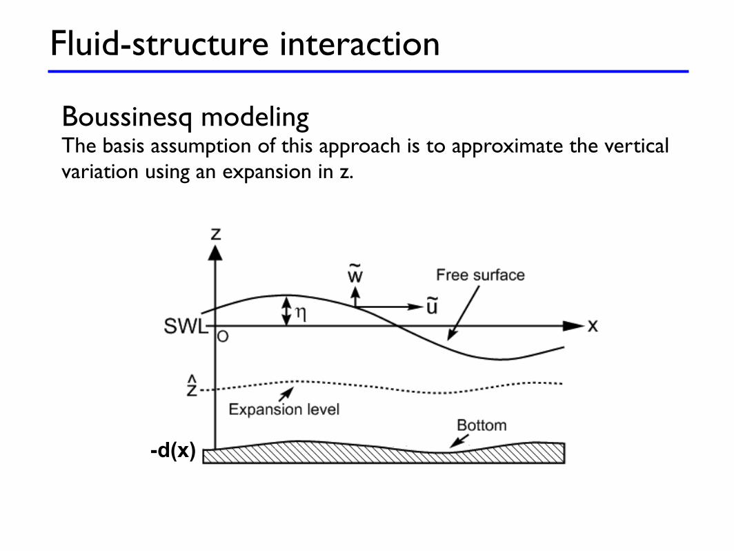
Fluid-structure interaction

Boussinesq modelingThe basis assumption of this approach is to approximate the vertical variation using an expansion in z.

-d(x)


Under certain assumptions, the proper model (a high-order Boussinesq model) becomes


Under certain assumptions, the proper model (a high-order Boussinesq model) becomes

2.1 Governing equations 11

where it has been assumed that d(x) has continuous first derivatives. At the free surface, wecan similarly determine a kinematic free surface condition by determining the rate of changeof z = !(x, t) as

"t! ! "z! + !! · !! =0 , z = !. (2.4)

We also need a dynamic free surface condition, which is given by Bernoulli’s equation havingset the atmospheric pressure to zero

"t! + g! +1

2

!

!! · !! +( "z!)2"

= 0, z = !. (2.5)

Following Zakharov (1968), Dommermuth and Yue (1987) and Witting (1984), the freesurface conditions can be reformulated by introducing variables defined directly at the freesurface

u " (!!)z=! , w " ("z!)z=! , ! " (!)z=! . (2.6)

The spatial and temporal di"erentiation of the free surface variables are by the chain rulegiven as

!! =( #!)z=! + ("z!)z=! !!,

"t! =( "t!)z=! + "t! ("z!)z=! ,

which by using Eq. (2.4) and Eq. (2.6) can be expressed as

U " !! = u + w!!, (2.7)

"t! =( "t!)z=! + w2 ! w!! · u. (2.8)

Now, we can reformulate the dynamic condition Eq. (2.5) using Eq. (2.7) and (2.8) into

"t! + g! +1

2

#

!! · !! ! w2(1 + !! · !!)$

= 0, (2.9)

and by applying the !-operator and changing notation we obtain

"tU + !

%

g! +1

2

#

U · U ! w2(1 + !! · !!)$&

= 0. (2.10)

Finally, the kinematic free surface condition Eq. (2.4) can be expressed as

"t! + !! · !! ! w (1 + !! · !!) = 0, (2.11)

or in the form used by Madsen et al. (2002) as

"t! ! w + !! ·#

U ! w!!$

= 0, (2.12)

which is then stated in terms of !, w and U .

2.1 Governing equations 11

where it has been assumed that d(x) has continuous first derivatives. At the free surface, wecan similarly determine a kinematic free surface condition by determining the rate of changeof z = !(x, t) as

"t! ! "z! + !! · !! =0 , z = !. (2.4)

We also need a dynamic free surface condition, which is given by Bernoulli’s equation havingset the atmospheric pressure to zero

"t! + g! +1

2

!

!! · !! +( "z!)2"

= 0, z = !. (2.5)

Following Zakharov (1968), Dommermuth and Yue (1987) and Witting (1984), the freesurface conditions can be reformulated by introducing variables defined directly at the freesurface

u " (!!)z=! , w " ("z!)z=! , ! " (!)z=! . (2.6)

The spatial and temporal di"erentiation of the free surface variables are by the chain rulegiven as

!! =( #!)z=! + ("z!)z=! !!,

"t! =( "t!)z=! + "t! ("z!)z=! ,

which by using Eq. (2.4) and Eq. (2.6) can be expressed as

U " !! = u + w!!, (2.7)

"t! =( "t!)z=! + w2 ! w!! · u. (2.8)

Now, we can reformulate the dynamic condition Eq. (2.5) using Eq. (2.7) and (2.8) into

"t! + g! +1

2

#

!! · !! ! w2(1 + !! · !!)$

= 0, (2.9)

and by applying the !-operator and changing notation we obtain

"tU + !

%

g! +1

2

#

U · U ! w2(1 + !! · !!)$&

= 0. (2.10)

Finally, the kinematic free surface condition Eq. (2.4) can be expressed as

"t! + !! · !! ! w (1 + !! · !!) = 0, (2.11)

or in the form used by Madsen et al. (2002) as

"t! ! w + !! ·#

U ! w!!$

= 0, (2.12)

which is then stated in terms of !, w and U .

18 Chapter 2. A high-order Boussinesq-type formulation

2.2 Boussinesq-type formulations

To summarize the results given in the former section, we show for clarity which equations weintend to solve. The starting point for the current work was the original velocity formulation,which we refer to as the rotational velocity formulation since by the approximation Eq. (2.13)the irrotational free assumption for the vorticity in the vertical is no longer required to besatisfied. However, with the intent to simplify the equations, Fuhrman (2004) re-introducedthe rotation free constraint, substituting !yu = !xv into the truncated equations, and as aside-e!ect found that the equation system became more stable numerically. We refer to thisformulation as the irrotational velocity formulation. Finally, Jamois et al. (2006) restatedand solved the high-order Boussinesq equation system numerically in terms of what we willrefer to as the potential formulation. The obvious advantage of the latter approach is thatthe number of unknowns and the complexity of the system reduces significantly leavingthe method much more attractive to solve numerically in comparison with the velocityformulations. However, the present work has primarily been based on the rotational versionas this formulation was used as the starting point for the current work.

2.2.1 Velocity formulations

The velocity formulations are given in terms of the exact free surface conditions Eq. (2.10)and Eq. (2.12) as

!t" = w ! !" ·!

U ! w!""

,

!tU = !!

#

g" +1

2

!

U · U ! w2(1 + !" · !")"$

,

and the vertical free surface velocity w can be determined in two steps by first solving forthe auxiliary variables u!, w! by solving both Eq. (2.7) and the kinematic condition at thesea bed Eq. (2.54) as a coupled system. The known values of U are related to the auxiliaryvariables through the definition in Eq. (2.7) combined with Eq. (2.50), Eq. (2.51). Fromthe solution we can determine w using Eq. (2.51). Using a compact notation this procedurefor the rotational velocity formulation amounts to first solving the 3x3 block system

%

&

UV0

'

( =

%

&

A11 ! !x" · B11 A2 ! !x" · B12 B11 + !x" · A1

A2 ! !y" · B11 A22 ! !y" · B12 B12 + !y" · A1

A01 + S01 A02 + S02 B0 + S03

'

(

%

&

u!

v!

w!

'

( , (2.58)

or for the irrotational formulation where the irrotational condition for the vertical vorticitycomponent !yu = !xv has been applied to simplify the equation system into

%

&

UV0

'

( =

%

&

A1 ! !x" · B11 !!x" · B12 B11 + !x" · A1

!!y" · B11 A1 ! !y" · B12 B12 + !y" · A1

A01 + S1 A02 + S2 B0 + S03

'

(

%

&

u!

v!

w!

'

( , (2.59)2.2 Boussinesq-type formulations 19

and then determine w from the solution of one of above using

w = !B11u! ! B12v

! + A1w!. (2.60)

The continuous di!erential operators characterized by the subscripted letters A, B, and Sare for brevity all given in Appendix A.

In the general case the global operators in Eq. (2.58) and Eq. (2.59) are unsymmetric andthe last row of block operators has no time-dependency. However, for the linearized versionof these operators, a flat sea bed, and an expansion level z = !0.5d the resulting globaloperators become block symmetric. As a result the kinematic condition at the sea bed (lastequation in Eq. (2.58) or (2.59)) can be added to Eq. (2.60) which then simplifies into asingle operation w = (A1 + B0)w!.

2.2.2 Potential formulation

The potential formulation is given in terms of the exact free surface conditions Eq. (2.9)and Eq. (2.11) as

!t" = !!" · !" + w (1 + !" · !") ,

!t" = !g" !1

2

!

!" · !" ! w2(1 + !" · !")"

.

As explained in the former subsection we can solve for the vertical free surface velocity wby a two step procedure, where the first step is to solve the Laplace problem in the interioras follows (notation deviates from the one used in Jamois et al. (2006))

#

"0

$

=

#

A1 B1

B2 + S3 B0 + S03

$ #

#!

w!

$

, (2.61)

and subsequently obtain the solution for w from

w = !B3#! + A1w

!. (2.62)

The continuous di!erential operators characterized by the subscripted letters A, B, and Sare for brevity all given in Appendix A.

Since the algebraic system Eq. (2.61) is expressed in terms of the scalar velocity potentialit therefore remains unchanged whether the problem is solved in one or two horizontaldimensions.

The potential formulation was recently presented and applied in Jamois et al. (2006). Thederivation for the potential formulation has been included in the former sections for com-pleteness, since it is considered to be more general than the equivalent velocity formulation.

Similar to the velocity formulations, the global operator in Eq. (2.61) is generally unsym-metric and the last row of block operators has no time-dependency.

Fluid-structure interactionWhere we have high-order derivates since

A bit on the complicated side !


Where we have high-order derivates since

Appendix A

Di!erential Boussinesq operators

A number of di!erential operators arise as a result of the derivation procedure for thehigh-order Boussinesq formulation given in Section 2.1. The definitions of these contin-uous di!erential operators for use with either of the three di!erent formulations in twohorizontal dimensions are given here for the Pade (4,4) versions. The Pade (2,2) versions arestraightforwardly obtained by truncating the high-order terms and changing the coe"cients!i, "i, #i, ci, si appropriately. The continuous operators are determined using the power rulesof ! given in Eq. (2.23). All coe"cients and variables used in the definitions have beenintroduced in Section 2.1. The operators for two horizontal dimensions reduce in the obviousway to the operators for one horizontal dimension.

The di!erential operators for the rotational velocity formulation are given as

A01 = $%x + #3$3(%xxx + %xyy) + #5$

5(%xxxxx + 2%xxxyy + %xyyyy), (A.1)

A02 = $%y + #3$3(%xxy + %yyy) + #5$

5(%xxxxy + 2%xxyyy + %yyyyy), (A.2)

A1 = 1 " !2(%xx + %yy) + !4(%xxxx + 2%xxyy + %yyyy), (A.3)

A11 = 1 " !2(%xx) + !4(%xxxx + %xxyy), (A.4)

A2 = "!2(%xy) + !4(%xxxy + %xyyy), (A.5)

A22 = 1 " !2(%yy) + !4(%xxyy + %yyyy), (A.6)

B0 = 1 + #2$2(%xx + %yy) + #4$

4(%xxxx + 2%xxyy + %yyyy), (A.7)

B11 = "1%x " "3(%xxx + %xyy) + "5(%xxxxx + 2%xxxyy + %xyyyy), (A.8)

B12 = "1%y " "3(%xxy + %yyy) + "5(%xxxxy + 2%xxyyy + %yyyyy), (A.9)

(A.10)

with the following operators for handling a mildly varying sea bed

S01 = %xd · C11 + %yd · C2, (A.11)

S02 = %xd · C2 + %yd · C22, (A.12)

S03 = "%xd · C13 " %yd · C23, (A.13)

159

Appendix A




A01 = $%x + #3$3(%xxx + %xyy) + #5$


A02 = $%y + #3$3(%xxy + %yyy) + #5$



A11 = 1 " !2(%xx) + !4(%xxxx + %xxyy), (A.4)

A2 = "!2(%xy) + !4(%xxxy + %xyyy), (A.5)

A22 = 1 " !2(%yy) + !4(%xxyy + %yyyy), (A.6)

B0 = 1 + #2$2(%xx + %yy) + #4$




(A.10)


S01 = %xd · C11 + %yd · C2, (A.11)

S02 = %xd · C2 + %yd · C22, (A.12)

S03 = "%xd · C13 " %yd · C23, (A.13)

159

Appendix A




A01 = $%x + #3$3(%xxx + %xyy) + #5$


A02 = $%y + #3$3(%xxy + %yyy) + #5$



A11 = 1 " !2(%xx) + !4(%xxxx + %xxyy), (A.4)

A2 = "!2(%xy) + !4(%xxxy + %xyyy), (A.5)

A22 = 1 " !2(%yy) + !4(%xxyy + %yyyy), (A.6)

B0 = 1 + #2$2(%xx + %yy) + #4$




(A.10)


S01 = %xd · C11 + %yd · C2, (A.11)

S02 = %xd · C2 + %yd · C22, (A.12)

S03 = "%xd · C13 " %yd · C23, (A.13)

159

160 Appendix A. Di!erential Boussinesq operators

where

C11 = 1 ! c2!2("xx) + c4!

4("xxxx + "xxyy), (A.14)

C2 = !c2!2("xy) + c4!

4("xxxy + "xyyy), (A.15)

C13 = !"x ! s3!3("xxx + "xyy) + s5!

5("xxxxx + 2"xxxyy + "xyyyy), (A.16)

C22 = 1 ! c2!2("yy) + c4!

4("xxyy + "yyyy), (A.17)

C23 = !"y ! s3!3("xxy + "yyy) + s5!

5("xxxxy + 2"xxyyy + "yyyyy). (A.18)

For the irrotational velocity formulation the operators for handling a mildly varying sea bedare given as

S1 = "xd · C1, (A.19)

S2 = "yd · C1, (A.20)

where

C1 = 1 ! c2!2("xx + "yy) + c4!

4("xxxx + 2"xxyy + "yyyy). (A.21)

In the potential formulation we have introduced the following di!erential operators

B1 = #1 ! #3("xx + "yy) + #5("xxxx + 2"xxyy + "yyyy), (A.22)

B2 = !("xx + "yy) + $3!3("xxxx + 2"xxyy + "yyyy)

+ $5!5("xxxxxx + 3"xxxxyy + 3"xxyyyy + "yyyyyy), (A.23)

B3 = #1("xx + "yy) ! #3("xxxx + 2"xxyy + "yyyy)

+ #5("xxxxxx + 3"xxxxyy + 3"xxyyyy + "yyyyyy), (A.24)

and the following additional operator for handling a mildly varying sea bed

S3 = "xd · C3 + "yd · C4, (A.25)

where

C3 = "x ! c2!2("xxx + "xyy) + c4!


C4 = "y ! c2!2("yyy + "xxy) + c4!


Note, that many of the terms involved in the di!erential operators above can be formedusing products of the Laplacian operator L = "xx + "yy. For example, the term "xxxxx +"xxxyy + "xyyyy = "x("xx + "yy)2, which appears in A01. This can be exploited in a practicalimplementation to reduce memory storage and increase e"ciency.

160 Appendix A. Di!erential Boussinesq operators

where

C11 = 1 ! c2!2("xx) + c4!

4("xxxx + "xxyy), (A.14)

C2 = !c2!2("xy) + c4!

4("xxxy + "xyyy), (A.15)

C13 = !"x ! s3!3("xxx + "xyy) + s5!


C22 = 1 ! c2!2("yy) + c4!

4("xxyy + "yyyy), (A.17)

C23 = !"y ! s3!3("xxy + "yyy) + s5!


For the irrotational velocity formulation the operators for handling a mildly varying sea bedare given as

S1 = "xd · C1, (A.19)

S2 = "yd · C1, (A.20)

where

C1 = 1 ! c2!2("xx + "yy) + c4!

4("xxxx + 2"xxyy + "yyyy). (A.21)

In the potential formulation we have introduced the following di!erential operators

B1 = #1 ! #3("xx + "yy) + #5("xxxx + 2"xxyy + "yyyy), (A.22)

B2 = !("xx + "yy) + $3!3("xxxx + 2"xxyy + "yyyy)

+ $5!5("xxxxxx + 3"xxxxyy + 3"xxyyyy + "yyyyyy), (A.23)

B3 = #1("xx + "yy) ! #3("xxxx + 2"xxyy + "yyyy)

+ #5("xxxxxx + 3"xxxxyy + 3"xxyyyy + "yyyyyy), (A.24)

and the following additional operator for handling a mildly varying sea bed

S3 = "xd · C3 + "yd · C4, (A.25)

where

C3 = "x ! c2!2("xxx + "xyy) + c4!


C4 = "y ! c2!2("yyy + "xxy) + c4!


Note, that many of the terms involved in the di!erential operators above can be formedusing products of the Laplacian operator L = "xx + "yy. For example, the term "xxxxx +"xxxyy + "xyyyy = "x("xx + "yy)2, which appears in A01. This can be exploited in a practicalimplementation to reduce memory storage and increase e"ciency.

A bit on the complicated side !

A couple of 2D(1D) testsSubmerged bar (K=110, P=8) - comparison with experimental data

A couple of 3D(2D) tests

x/L

y/L

-2 -1 0 1 2 3 4-2

-1

0

1

2

0

0.2

0.4

0.6

0.8

1

1.2

1.4

1.6

1.8

x/L

y/L

-2 -1 0 1 2 3 4-2

-1

0

1

2

00.20.40.60.811.21.41.61.8

0.5

1

1.5

2

30

210

60

240

90

270

120

300

150

330

180 0

Max. wave runup (ka=3.1)

θ

Emax/

(H/2)

0.5

1

1.5

2

30

210

60

240

90

270

120

300

150

330

180 0

θ

ηmax/

(H/2)

McCamy & Fuchs (1954)

DG-FEM solution:ka=pi, kd=1.0,P=4, K=1261, t=0.03s

Compressible fluid flow

Time-dependent Euler equations

• Gas• High speed• etc

Formulation is straightforward

Challenge: Shocks -- this requires limiting/filtering



• Gas

• High speed

• etc


100

101

102

10!8

10!7

10!6

10!5

10!4

10!3

10!2

10!1

100

K1/2

||E!Eh||

N=1

N=2

N=3

N=4

N=5

100

101

102

10!8

10!7

10!6

10!5

10!4

10!3

10!2

10!1

100

K1/2

||E!Eh||

N=1

N=2

N=3

N=4

N=5

Fig. 6.9. On the left is shown the discrete L2-error for Ezh at T = 10, obtained using a DG-FEM with

central fluxes, for di!erent values of N and K. As a measure of average cell size, we use!

K. On the rightwe show similar results obtained using an upwind flux.

!"u

!t+

!"u2 + p

!x+

!"uv

!y= 0,

!"v

!t+

!"uv

!x+

!"v2 + p

!y= 0,

!E

!t+

!u (E + p)!x

+!v (E + p)

!y= 0,

where " is the density of the gas, ("u, "v) are the x- and y-components of the momentum, p isthe internal pressure of the gas, and E is the total energy of the gas. The total energy of the gasis the sum of the potential energy due to the internal pressure and the kinetic energy due to itsmomentum, given by

E =p

# ! 1+

"

2!u2 + v2

",

where # is a constant dependent on the type of gas. For this example, we will consider a monoatomicgas with # = 1.4. The above equations neglect the e!ects of viscosity and thermal di!usion, whichwe will be incorporated into a later example that concerns the Navier-Stokes equations for a com-pressible fluid (see Section 7.5).

To provide some insight into a relatively general numerical discretization for a wide class ofnonlinear conservation laws, with Euler’s equations as the guiding example, we rewrite the equationsin vector form:

!q!t

+!F!x

+!G!y

= 0,

where

q =

#

$$%

""u"vE

&

''( , F =

#

$$%

"u"u2 + p

"uvu (E + p)

&

''( , G =

#

$$%

"v"uv

"v2 + pv (E + p)

&

''( ,

6.6 Compressible gas dynamics 193

represent the state vector and the two nonlinear fluxes, respectively. These vector flux functionsare implemented in a straightforward manner by first extracting the primitive variables (!, u, v, p)from the conserved variable state vector q at each volume element node in EulerFluxes2D.m. Wehave chosen to store the state vector as a three-dimensional array, Q, of size Np !K ! 4, with thelast dimension being the number of conserved variables.

EulerFluxes2D.m

6 % extract conserved variables7 rho = Q(:,:,1); rhou = Q(:,:,2); rhov = Q(:,:,3); Ener = Q(:,:,4);8

9 % compute primitive variables10 u = rhou./rho; v = rhov./rho; p = (gamma-1)*(Ener - 0.5*(rhou.*u + rhov.*v));

Combinations of the primitive and conserved variables are then used to evaluate the vector fluxfunctions F and G in a straightforward manner.

EulerFluxes2D.m

12 % compute flux functions13 F = zeros(size(Q));14 F(:,:,1) = rhou; F(:,:,2) = rhou.*u + p; F(:,:,3) = rhov.*u; F(:,:,4) = u.*(Ener+p);15

16 G = zeros(size(Q));17 G(:,:,1) = rhov; G(:,:,2) = rhou.*v; G(:,:,3) = rhov.*v + p; G(:,:,4) = v.*(Ener+p);

Following the previous discussions, we represent the state vector as a piecewise N -th-orderpolynomial, qh, and require it to satisfy a DG statement on weak form for all test functions "h " Vh,as !

Dk

"#qh

#t"h # Fh

#"h

#x#Gh

#"h

#y

#dx +

$

!Dk(nxFh + nyGh)! "hdx = 0.

For the numerical flux, we use the local Lax-Friedrichs flux

(nxFh + nyGh)! = nx{{Fh}} + ny{{Gh}} +$

2· [[qh]].

The dissipative nature of this flux will smear shocks in strongly supersonic and transitional flows butwill serve adequately for most subsonic and weakly supersonic flows. To complete the computationof the fluxes, we recover an approximate local maximum linearized acoustic wave speed

$ = maxs"[q!h ,q+

h ]

%|u(s)| +

&''''%p(s)!(s)

''''

(.

EulerRHS2D.m contains an implementation of the right-hand-side terms. First, we compute thevolume terms for each component of the state vector, taking advantage of the local di!erentiationmatrices common to all elements and applying the chain rule to compute the Cartesian derivativesof the fields.



EulerFluxes2D.m




EulerFluxes2D.m




Dk

"#qh

#t"h # Fh

#"h

#x#Gh

#"h

#y

#dx +

$




2· [[qh]].


$ = maxs"[q!h ,q+

h ]

%|u(s)| +

&''''%p(s)!(s)

''''

(.






• Gas

• High speed

• etc


100

101

102

10!8

10!7

10!6

10!5

10!4

10!3

10!2

10!1

100

K1/2

||E!Eh||

N=1

N=2

N=3

N=4

N=5

100

101

102

10!8

10!7

10!6

10!5

10!4

10!3

10!2

10!1

100

K1/2

||E!Eh||

N=1

N=2

N=3

N=4

N=5

Fig. 6.9. On the left is shown the discrete L2-error for Ezh at T = 10, obtained using a DG-FEM with

central fluxes, for di!erent values of N and K. As a measure of average cell size, we use!

K. On the rightwe show similar results obtained using an upwind flux.

!"u

!t+

!"u2 + p

!x+

!"uv

!y= 0,

!"v

!t+

!"uv

!x+

!"v2 + p

!y= 0,

!E

!t+

!u (E + p)!x

+!v (E + p)

!y= 0,

where " is the density of the gas, ("u, "v) are the x- and y-components of the momentum, p isthe internal pressure of the gas, and E is the total energy of the gas. The total energy of the gasis the sum of the potential energy due to the internal pressure and the kinetic energy due to itsmomentum, given by

E =p

# ! 1+

"

2!u2 + v2

",

where # is a constant dependent on the type of gas. For this example, we will consider a monoatomicgas with # = 1.4. The above equations neglect the e!ects of viscosity and thermal di!usion, whichwe will be incorporated into a later example that concerns the Navier-Stokes equations for a com-pressible fluid (see Section 7.5).

To provide some insight into a relatively general numerical discretization for a wide class ofnonlinear conservation laws, with Euler’s equations as the guiding example, we rewrite the equationsin vector form:

!q!t

+!F!x

+!G!y

= 0,

where

q =

#

$$%

""u"vE

&

''( , F =

#

$$%

"u"u2 + p

"uvu (E + p)

&

''( , G =

#

$$%

"v"uv

"v2 + pv (E + p)

&

''( ,



EulerFluxes2D.m




EulerFluxes2D.m




Dk

"#qh

#t"h # Fh

#"h

#x#Gh

#"h

#y

#dx +

$




2· [[qh]].


$ = maxs"[q!h ,q+

h ]

%|u(s)| +

&''''%p(s)!(s)

''''

(.




EulerFluxes2D.m




EulerFluxes2D.m




Dk

"#qh

#t"h # Fh

#"h

#x#Gh

#"h

#y

#dx +

$




2· [[qh]].


$ = maxs"[q!h ,q+

h ]

%|u(s)| +

&''''%p(s)!(s)

''''

(.






Density

Density

Density

Density

Fig. 6.14. Sequence of solutions to the Mach 3 forward facing step test case (with uniformly refined meshesof size K=381, 1524, 6096, and 24384) using the Tu and Aliabadi limiter with an N = 1 DG method. Thirtyequally spaced Mach contours are plotted in the range [0.090388, 6.2365].

extension of this result to the multidimensional case is, as it turns out, technically more complexthan the one-dimensional case, but the main results remain unchanged with one essential exception.

The analysis of the error estimates for linear problems is typically done for the equation

! ·!u + !u = f, x " " # R2,

which is in fact the neutron transport equation for which the first DG-FEM was introduced in [269].In early work [217], it was shown that if u is smooth and " is tiled with rectangular elements, eachusing an N -th-order tensor basis, the scheme exhibits optimal convergence; that is,

Remarks

We are done with all the basic now ! -- and we have started to see it work for us

What we need to worry about is:

✓The need for 3D✓The need for speed✓Software beyond Matlab

Tomorrow !

Documents

DG-FEM for PDE’s Lecture 7 - Technical University of …apek/DGFEMCourse2009/Lecture07.pdf · DG-FEM for PDE’s Lecture 7 ... Introduction and DG-FEM in 1D • Lecture 2: Implementation