DFT calculations of NMR indirect spin–spin coupling constants

•  Dalton program system –  Program capabilities

•  Density functional theory –  Kohn–Sham theory –  LDA, GGA and hybrid theories

•  Indirect NMR spin–spin coupling constants –  Ramsey’s second-order expression –  Computational aspects

•  Calculation of spin–spin coupling constants –  Comparison with high-level ab initio methods

Dalton program system •  Electronic-structure program system

–  developed mostly in Scandinavia (Aarhus, Odense, Oslo and Stockholm) –  http://www.kjemi.uio.no/software/dalton

•  Computational methods –  Hartree–Fock –  multiconfigurational self-consistent field (MCSCF) –  coupled-cluster theory –  density-functional theory

•  Properties –  geometry optimizations and trajectories –  vibrational spectra (frequencies and intensities) –  excitation energies (triplet and singlet) –  static and dynamic polarizabilities and hyperpolarizabilities –  magnetic properties

•  570 licenses worldwide

Density functional theory •  The energy is expressed as a functional of the electron density r:

•  The interaction with the external potential simple:

•  By contrast, the kinetic energy T[ρ] and electron–electron repulsion energy Vee[ρ] are difficult to calculate.

•  However, an important, simple contribution to Vee[ρ] is the electron– electron Coulomb repulsion energy:

Noninteracting electrons •  For a system of noninteracting electrons, we may write the density as

•  In this case, the total energy may be written in the form

where the kinetic energy is evaluated exactly as

•  and the orbitals satisfy the eigenvalue equations

Kohn–Sham theory

Kohn–Sham and Hartree–Fock theories •  With the density in the form , we have now expressed

the DFT (Kohn–Sham) energy in the form

which is similar to that of the Hartree–Fock energy

•  The optimization may therefore be carried out in the same manner, replacing the Fock potential by the exchange–correlation potential

•  In practice, the evaluation of Exc[ρ] involves adjustable parameters; we may thus regard Kohn–Sham theory as semi-empirical Hartree– Fock theory.

LDA theory

•  The true form of the exchange–correlation functional is unknown and is presumably a complicated, nonlocal function of the electron density.

•  However, reasonable results are obtained by assuming that the functional depends only locally on the density.

•  In the local-density approximation (LDA), we use Dirac’s (nonempirical) expression for the exchange energy

•  For the correlation energy, the Vosko–Wilk–Nusair (VWN) functional (1980) is used; it is based on electron-gas simulations and contains three adjustable parameters.

GGA theory •  For quantitative results, it is necessary to include corrections from the

gradient of the density such as

•  With such gradient corrections included, we arrive at the generalized gradient-approximation (GGA) level of theory.

•  The popular BLYP method uses –  Becke’s gradient correction to the exchange (1988)

•  one parameter adjusted to reproduce the exchange energy of the six noble-gas atoms

–  the correlation correction due to Lee, Yang and Parr (1988) •  four parameters adjusted to reproduce the correlation energy of the helium atom

Hybrid DFT theories

•  A successful Kohn–Sham approach has been to include some proportion of the exact Hartree–Fock exchange in the calculations: hybrid DFT

•  In particular, the B3LYP functional contains the following contributions

where the parameters have been fixed in a highly semi-empirical manner.

•  B3LYP performs remarkably well in many circumstances – for example, for the calculation of molecular structure, vibrational frequencies, atomization energies, and excitations.

•  In the following, we shall concern ourselves with indirect NMR spin–spin coupling constants.

Implementation of DFT

•  In an existing ab initio code such as Dalton, Kohn–Sham theory may be implemented as an extension to Hartree–Fock theory.

•  Wherever it appears, the Hartree–Fock exchange contribution is replaced by a contribution from the exchange–correlation functional:

–  total energy –  Kohn–Sham matrix –  linear Hessian transformations

•  In hybrid theories, the Hartree–Fock exchange is scaled rather than removed.

•  The evaluation of the exchange–correlation contributions involves an integration over all space:

–  numerical scheme more convenient than an analytical one –  the space is divided into regions surrounding each nucleus –  within each such region, a one-dimensional radial and two-dimensional

angular quadrature is carried out

Implementation in Dalton

•  The implementation in Dalton is based on that in Cadpac –  it uses the same code for generating quadrature points and weights –  many of the same routines for the functionals

•  Features of the implementation –  restricted Kohn–Sham theory only –  full use of Abelian point-group symmetry –  parallelization over quadrature points –  generally contracted spherical-harmonic Gaussians

•  The functional evaluation scales as KN2, where K is the number of atoms and N the number of AOs.

Features of Dalton DFT •  Functionals:

–  LDA, BLYP, B3LYP –  other functionals may be easily added

•  Properties: –  total electronic energies –  molecular forces (and thus first-order geometry optimizations) –  multipole moments and other expectation values –  RPA singlet and triplet excitation energies –  NMR shieldings (with and without London orbitals) –  NMR indirect spin–spin coupling constants –  static and dynamic polarizabilities –  magnetizabilities and molecular Hessians require some simple coding

•  Planned for Dalton 2.0 release

NMR nuclear spin–spin couplings

•  In NMR, we observe direct and indirect couplings between the magnetic moments of paramagnetic nuclei

•  Within the Born–Oppenheimer approximation, these couplings may be calculated as second-order time-independent properties

•  Because of the smallness of the moments (10-3) and their coupling to the electrons (10-5), these constants are extremely small: ~10-16Eh

NMR spectra

Nuclear magnetic perturbations •  Perturbed nonrelativistic electronic Hamiltonian:

•  The nuclear magnetic vector potential

gives rise to a first-order imaginary singlet perturbation and a second-order real singlet perturbation

•  The nuclear magnetic induction

gives rise to a first-order real triplet perturbation.

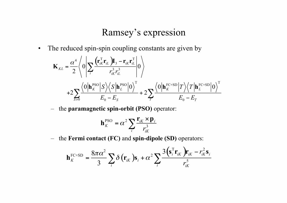
Ramsey’s expression •  The reduced spin-spin coupling constants are given by

–  the paramagnetic spin-orbit (PSO) operator:

–  the Fermi contact (FC) and spin-dipole (SD) operators:

Calculation of spin–spin couplings •  In practice, second-order properties are not calculated from sum-over-

states expressions •  Instead, the coupling constants are calculated from the expression

•  Here λS and λT represent singlet and triplet variations of the electronic state, whose responses are obtained by solving the linear equations

and similarly for the triplet perturbations. •  These response equations are solved iteratively, without constructing

the Hessian matrices explicitly

NMR indirect nuclear spin–spin couplings

•  The calculation of NMR spin-spin coupling constants is a very demanding task: –  requires a highly flexible wave function to describe the triplet perturbations

induced by the nuclear magnetic moments (triplet instabilities problems) –  large basis sets with a flexible inner core needed –  for each paramagnetic nucleus, we must solve at least nine response

equations: •  3 imaginary singlet perturbations •  6 real triplet perturbations

•  Standard ab initio approaches: –  RHF gives notoriously poor results –  CCSD is qualitatively but not quantitatively correct –  CCSD(T) not useful –  MCSCF and SOPPA are probably the most successful methods so far

•  Different DFT in HIII basis compared with RHF and full-valence CAS

•  LDA represents a significant improvement on RHF •  Whereas RHF overestimates couplings, LDA underestimates them •  BLYP increases couplings and improves agreement somewhat •  Significant improvement at the B3LYP level

DFT spin-spin methods compared

Contributions to spin-spin couplings •  In Ramsey’s treatment, there are four contributions to the couplings. •  Usually, the most important is FC and the least important DSO. •  A priori, none of the couplings can be neglected.

Couplings compared (Hz)

Karplus relation •  The nuclear spin-spin couplings are extremely sensitive to geometries. •  Important special case: the Karplus relation between vicinal coupling

constants and the dihedral angle φ between two CH bonds •  Below, we compare the B3LYP/HIII curve with an empirical curve

Conclusions

•  For the calculation of indirect NMR spin –spin coupling constants, LDA is a vast improvement on Hartree–Fock theory –  no triplet-instability problems –  indirect nuclear spin–spin couplings underestimated

•  Some improvement observed at the GGA (BLYP) level •  B3LYP in semi-quantitative agreement with experiment

–  typical errors less than 10% –  matches the best ab initio results (MCSCF, SOPPA, and CCSD) –  will presumably be no match for CCSDT –  may be applied to large systems –  cannot be systematically improved