Embed Size (px)
Citation preview

Developments in The Extended Finite Element Method & AlgebraicMultigrid for Solid Mechanics Problems Involving Discontinuities
Badri Krishna Jainath Hiriyur
Submitted in partial fulfillment of therequirements for the degree of
Doctor of Philosophyin the Graduate School of Arts and Sciences
COLUMBIA UNIVERSITY
2012

c© 2012
Badri Krishna Jainath Hiriyur
All rights reserved.

Abstract
Developments in The Extended Finite Element Method & Algebraic Multigridfor Solid Mechanics Problems Involving Discontinuities
Badri Krishna Jainath Hiriyur
In this dissertation, some contribututions related to computational modeling and solution of solid
mechanics problems involving discontinuities are discussed. The main tool employed for dis-
crete modeling of discontinuities is the extended finite element method and the primary solution
method discussed is the algebraic multigrid. The extended finite element method has been shown
to be effective for both weak and strong discontinuities. With respect to weak discontinuities,
a new approach that couples the extended finite element method with Monte Carlo simulations
with the goal of quantifying uncertainty in homogenization of material properties of random mi-
crostructures is presented. For accelearated solution of linear systems arising from problems in-
volving cracks, several new methods involving the algebraic multigrid are presented. In the first
approach, the Schur complement of the linear system arising from XFEM is used to develop a
Hybrid-AMG method such that crack-conforming aggregates are formed. Another alternative ap-
proach involves transforming the original linear system into a modified system that is amenable
for a direct application of algebraic multigrid. It is shown that if only Heaviside-enrichments
are present, a simple transformation based on the phantom-node approach is available, which
decouples the linear sysem along the discontinuities such that crack conforming aggregates are
automatically generated via smoother aggregation algebraic multigrid. Various numerical exam-
ples are presented to verify the accuracy of the resuting solutions and the convergence properties
of the proposed algorithms. The parallel scalability performance of the implementation are also
discussed.
Contents
Contents i
List of Tables v
List of Figures vii
Acknowledgements xi
I Introduction 1
1 Scope-Outline 2
1.1 Introduction . . . . . . . . . . . . . . . . . . . . . . . . . . . . . . . . . . . . . . . . . . 2
1.2 Outline . . . . . . . . . . . . . . . . . . . . . . . . . . . . . . . . . . . . . . . . . . . . . 2
II Weak Discontinuities 5
2 State-of-the-art 6
2.1 Motivation & Literature Survey . . . . . . . . . . . . . . . . . . . . . . . . . . . . . . . 6
3 XFEM-Inclusions 11
3.1 XFEM for Weak Discontinuities . . . . . . . . . . . . . . . . . . . . . . . . . . . . . . . 11
3.1.1 Fundamental equations . . . . . . . . . . . . . . . . . . . . . . . . . . . . . . . 11
3.1.2 Enrichment function . . . . . . . . . . . . . . . . . . . . . . . . . . . . . . . . . 15
3.1.3 Convergence study of XFEM solution for single inclusion . . . . . . . . . . . 16
3.1.4 Convergence study of XFEM solution for multiple inclusions . . . . . . . . . 21
4 XFEM-MC 25
4.1 Monte Carlo approach . . . . . . . . . . . . . . . . . . . . . . . . . . . . . . . . . . . . 25
i

4.1.1 Random microstructure generation . . . . . . . . . . . . . . . . . . . . . . . . 26
4.2 Homogenization . . . . . . . . . . . . . . . . . . . . . . . . . . . . . . . . . . . . . . . 27
4.2.1 Application and results . . . . . . . . . . . . . . . . . . . . . . . . . . . . . . . 27
4.2.2 Discussion . . . . . . . . . . . . . . . . . . . . . . . . . . . . . . . . . . . . . . . 40
4.3 Concluding remarks . . . . . . . . . . . . . . . . . . . . . . . . . . . . . . . . . . . . . 40
III Strong Discontinuities 42
5 Introduction 43
5.1 Motivation & Literature Survey . . . . . . . . . . . . . . . . . . . . . . . . . . . . . . . 43
5.2 XFEM for Strong Discontinuities . . . . . . . . . . . . . . . . . . . . . . . . . . . . . . 46
5.2.1 Governing Equations . . . . . . . . . . . . . . . . . . . . . . . . . . . . . . . . . 46
5.2.2 Weak Form . . . . . . . . . . . . . . . . . . . . . . . . . . . . . . . . . . . . . . 47
5.2.3 Levelset Functions . . . . . . . . . . . . . . . . . . . . . . . . . . . . . . . . . . 49
5.2.4 XFEM Linear System . . . . . . . . . . . . . . . . . . . . . . . . . . . . . . . . . 51
5.3 Algebraic Multigrid . . . . . . . . . . . . . . . . . . . . . . . . . . . . . . . . . . . . . . 53
5.4 AMG for XFEM . . . . . . . . . . . . . . . . . . . . . . . . . . . . . . . . . . . . . . . . 58
6 XAMG-I 60
6.1 Schur complement of XFEM matrix . . . . . . . . . . . . . . . . . . . . . . . . . . . . . 60
6.2 A new AMG method . . . . . . . . . . . . . . . . . . . . . . . . . . . . . . . . . . . . . 64
6.3 Algorithm Details . . . . . . . . . . . . . . . . . . . . . . . . . . . . . . . . . . . . . . . 68
6.4 Numerical Results . . . . . . . . . . . . . . . . . . . . . . . . . . . . . . . . . . . . . . . 72
6.4.1 Application in 3D . . . . . . . . . . . . . . . . . . . . . . . . . . . . . . . . . . . 76
6.5 Extensions . . . . . . . . . . . . . . . . . . . . . . . . . . . . . . . . . . . . . . . . . . . 78
7 XAMG-II 79
7.1 Introduction . . . . . . . . . . . . . . . . . . . . . . . . . . . . . . . . . . . . . . . . . . 79
7.2 Phantom node representation . . . . . . . . . . . . . . . . . . . . . . . . . . . . . . . . 80
7.2.1 Choice of enrichment form . . . . . . . . . . . . . . . . . . . . . . . . . . . . . 82
ii

7.2.2 Transformation . . . . . . . . . . . . . . . . . . . . . . . . . . . . . . . . . . . . 84
7.2.3 Modified null space . . . . . . . . . . . . . . . . . . . . . . . . . . . . . . . . . 85
7.3 Implementation . . . . . . . . . . . . . . . . . . . . . . . . . . . . . . . . . . . . . . . . 86
7.4 Numerical Results . . . . . . . . . . . . . . . . . . . . . . . . . . . . . . . . . . . . . . . 87
7.4.1 Linear elastic solves in serial . . . . . . . . . . . . . . . . . . . . . . . . . . . . 87
7.4.2 Plasticity solves in serial . . . . . . . . . . . . . . . . . . . . . . . . . . . . . . . 89
7.5 Summary and Conclusions . . . . . . . . . . . . . . . . . . . . . . . . . . . . . . . . . 92
IV Conclusions 93
8 Summary 94
8.1 Main Contributions . . . . . . . . . . . . . . . . . . . . . . . . . . . . . . . . . . . . . . 94
Bibliography 96
A XFEM-AMG-DD 105
A.1 Introduction . . . . . . . . . . . . . . . . . . . . . . . . . . . . . . . . . . . . . . . . . . 105
A.2 Multiplicative Schwarz . . . . . . . . . . . . . . . . . . . . . . . . . . . . . . . . . . . . 106
A.3 setup-algorithm . . . . . . . . . . . . . . . . . . . . . . . . . . . . . . . . . . . . . . . . 111
A.4 Representative Example . . . . . . . . . . . . . . . . . . . . . . . . . . . . . . . . . . . 113
A.4.1 Multiple cracks with different lengths and orientations . . . . . . . . . . . . . 113
B XFEM-GA 116
B.1 Introduction . . . . . . . . . . . . . . . . . . . . . . . . . . . . . . . . . . . . . . . . . . 116
B.2 XFEM approach for solution of the forward problem . . . . . . . . . . . . . . . . . . . 117
B.2.1 Convergence of elliptical enrichment . . . . . . . . . . . . . . . . . . . . . . . 118
B.3 GA - XFEM based Identification . . . . . . . . . . . . . . . . . . . . . . . . . . . . . . . 118
B.3.1 Applied Weighted Average Mutation GA (WAM-GA) . . . . . . . . . . . . . . 123
B.4 Representative Example . . . . . . . . . . . . . . . . . . . . . . . . . . . . . . . . . . . 123
B.4.1 Identification of a crack using the elliptical inclusion XFEM-GA scheme . . . 123
iii

C XICE 127
C.1 FEAP User Element for 3D XFEM . . . . . . . . . . . . . . . . . . . . . . . . . . . . . . 127
C.1.1 Input format . . . . . . . . . . . . . . . . . . . . . . . . . . . . . . . . . . . . . . 128
C.1.2 Stiffness generation for jump-enriched element . . . . . . . . . . . . . . . . . . 128
iv

List of Tables
3.1 Problem size comparison . . . . . . . . . . . . . . . . . . . . . . . . . . . . . . . . . . . 23
4.1 Stiff circular inclusions: Statistics of Ee f f . . . . . . . . . . . . . . . . . . . . . . . . . . 32
4.2 Stiff elliptical inclusions: Statistics of Ee f f . . . . . . . . . . . . . . . . . . . . . . . . . 33
4.3 Soft elliptical inclusions: Statistics of Ee f f . . . . . . . . . . . . . . . . . . . . . . . . . 33
6.1 PCG iterations for different AMG approaches on a six crack problem (case 5b in
Figure 6.3i). . . . . . . . . . . . . . . . . . . . . . . . . . . . . . . . . . . . . . . . . . . 63
6.2 Assessment of Schur complement approximations for case 5a in Figure 6.3i . . . . . 70
6.3 Preconditioned CG iterations for two-dimensional problems . . . . . . . . . . . . . . 75
6.4 AMG operator complexities for Quasi AMG on Case 5b. . . . . . . . . . . . . . . . . 76
6.5 Preconditioned CG iterations for a three-dimensional problem . . . . . . . . . . . . . 77
6.6 AMG operator complexities for a three-dimensional problem . . . . . . . . . . . . . . 77
7.1 Comparison of different solvers: Direct, CG (unpreconditioned, “black-box” AMG
preconditioned and “XAMG” preconditioned). The number of pre- and post- sweeps
of symmetric Gauss-Seidel smoother is also varied (S1 and S5) for the precondi-
tioner. “nits” is the number of CG iterations and cpu time is measured in seconds . . 89
7.2 Solution of a fracture problem involving plasticity using CG-brute . . . . . . . . . . 91
7.3 Solution of a fracture problem involving plasticity using “black-box” AMG-S1 . . . . 91
7.4 Solution of a fracture problem involving plasticity using XAMG-S1 . . . . . . . . . . 91
A.1 Summary of the convergence results for the problem considered in Fig. A.4. . . . . . 115
v

B.1 WAM-GA scheme . . . . . . . . . . . . . . . . . . . . . . . . . . . . . . . . . . . . . . . 126
vi

List of Figures
2.1 (a,b) Scanning Electron Microscope micrographs of ceramic matrix composite from
Fair et. al. [21] (c) SEM micrograph of carbon nanotubes from Zhang et. al. [85] . . . 7
2.2 Multiscale information-passing approach: (a) composites scale (b) fiber scale (c)
coating scale (d) nanotube scale . . . . . . . . . . . . . . . . . . . . . . . . . . . . . . 8
3.1 Multiple inclusions within element boundary . . . . . . . . . . . . . . . . . . . . . . 12
3.2 Multiple inclusions (a) Enriched element (b) Enriched DOF . . . . . . . . . . . . . . 13
3.3 The two coordinate systems . . . . . . . . . . . . . . . . . . . . . . . . . . . . . . . . . 16
3.4 Enrichment function for an elliptical inclusion within an element: (a) ϕ(x), (b) Con-
tour levels of ϕ(x), (c) ∂ϕ∂x , (d) ∂ϕ
∂y . . . . . . . . . . . . . . . . . . . . . . . . . . . . . . 17
3.5 Schematic of load and boundary conditions . . . . . . . . . . . . . . . . . . . . . . . 18
3.6 Displacement solution comparison (a) XFEM mesh (b) XFEM displacements (c)
FEM mesh (d) FEM displacements . . . . . . . . . . . . . . . . . . . . . . . . . . . . . 19
3.7 Convergence of XFEM results to FEM results . . . . . . . . . . . . . . . . . . . . . . . 20
3.8 Effect of elastic moduli ratio on accuracy of XFEM solution . . . . . . . . . . . . . . 22
3.9 Mesh discretization: (a) ABAQUS FEM model (b) MATLAB XFEM model . . . . . . 23
3.10 Convergence of XFEM results to benchmark FEM results for the case of multiple
inclusions: (a) Convergence of x displacements along right edge (b) Relative norm
of the difference in edge displacements versus XFEM element size . . . . . . . . . . . 24
4.1 Sample realizations of generated random microstructures . . . . . . . . . . . . . . . . 28
vii

4.2 Boundary Conditions (arrows here indicate enforced displacements) . . . . . . . . . 31
4.3 Stiff circular inclusions: (a) Ee f f versus λ, (b) Histograms of Ee f f , (c) Ee f f versus np . 34
4.4 Stiff circular inclusions: Convergence of Mean and COV of Ee f f . . . . . . . . . . . . 35
4.5 Stiff elliptical inclusions: (a) Ee f f versus λ, (b) Histograms of Ee f f , (c) Ee f f versus np 36
4.6 Stiff elliptical inclusions: Convergence of Mean and COV of Ee f f . . . . . . . . . . . 37
4.7 Soft elliptical inclusions: (a) Ee f f versus λ, (b) Histograms of Ee f f , (c) Ee f f versus np 38
4.8 Soft elliptical inclusions: Convergence of Mean and COV of Ee f f . . . . . . . . . . . 39
5.1 2D Fracture domain . . . . . . . . . . . . . . . . . . . . . . . . . . . . . . . . . . . . . 47
5.2 (a) Thick lines (red) depict cracks. Circles (green) and squares (red) give nodes
enriched by H(x) and FJ(x), respectively. (b) Computed stress σyy. . . . . . . . . . . 49
5.3 Levelset functions for a single crack effectively subdividing Ω into 4 regions. . . . . 50
5.4 Levelsets in three dimensions (a) Mesh with crack (b) Φn contours (c) Ψn contours . 51
5.5 (a) XFEM mesh for a single crack (b) Sparsity pattern of A (c) Sparsity pattern of Axx 52
5.6 Multigrid V-cycle . . . . . . . . . . . . . . . . . . . . . . . . . . . . . . . . . . . . . . . 54
5.7 Multigrid V cycle consisting of ` levels to solve A[0]u[0] = b[0], where level 0 is the
finest level. . . . . . . . . . . . . . . . . . . . . . . . . . . . . . . . . . . . . . . . . . . 54
5.8 Basis functions and sine wave representation. . . . . . . . . . . . . . . . . . . . . . . . 56
5.9 Convergence of CG with and without preconditioning . . . . . . . . . . . . . . . . . 59
6.1 Graphic illustration of Schur complement stencil just left of a crack. . . . . . . . . . 62
6.2 Sparsity Pattern Modification: Blue circles indicate sparsity pattern of a single pro-
longator column and black squares are removed pattern entries due to a crack. . . . 69
6.3 Test crack configurations (1a,b,c) Single propagating crack (2a,b) Two edge cracks
(3a,b) Six edge cracks (4) Six interior cracks (5a,b) Inclined cracks . . . . . . . . . . . 73
6.4 Sample aggregates. Each grid point is colored corresponding to the aggregate that
contains it. The red lines represent cracks. . . . . . . . . . . . . . . . . . . . . . . . . . 74
viii

6.5 (a) XFEM 3D mesh for a three crack problem (b) XFEM solution - displacement
contours . . . . . . . . . . . . . . . . . . . . . . . . . . . . . . . . . . . . . . . . . . . . 77
7.1 Phantom node representation. Shaded regions (Ωa and Ωb) indicate basis function
support. . . . . . . . . . . . . . . . . . . . . . . . . . . . . . . . . . . . . . . . . . . . . 80
7.2 Shape functions for a phantom node representation . . . . . . . . . . . . . . . . . . . 81
7.3 Sparsity pattern of the stiffness matrix for phantom node representation . . . . . . . 81
7.4 Shape functions and enrichments (a) Standard bilinear shape function (b) Original
XFEM Heaviside enrichment (c) Shifted enrichment (d) Modified shifted enrich-
ment . . . . . . . . . . . . . . . . . . . . . . . . . . . . . . . . . . . . . . . . . . . . . . 83
7.5 Representative examples. Tip enrichments are not used in any of the examples
shown. Stress contours correspond to Von Mises stress. . . . . . . . . . . . . . . . . . 88
7.6 Simulation involving plasticity: Von Mises stress contours . . . . . . . . . . . . . . . 90
A.1 Schematic representation of the “healthy” and “cracked” subdomains in the formula-
tion of domain decomposition. [a] multiple cracks share a single cracked subdomain
[b] each crack is assigned to a different cracked subdomain. . . . . . . . . . . . . . . . 107
A.2 Two overlapping domains employed in the Schwarz method. The following color
legend is used: black squares represent Schwarz essential boundary conditions, the
black triangles represent clamped nodes, the red circles represent pulled nodes, the
green zone represent the elements belonging to the same subdomain, the blue zone
represent the elements that are part of the overlapping layer. . . . . . . . . . . . . . . 108
A.3 Schematic description of the inexact Schwarz-AMG preconditioner . . . . . . . . . . 112
A.4 Domain decomposition and mesh of a plate with three cracks with different lengths
and orientations [a] Decomposition with multiple cracked subdomains [b] Decom-
position with a single cracked subdomain. . . . . . . . . . . . . . . . . . . . . . . . . . 113
A.5 Comparison of the convergence rate for the decomposition strategies shown in Fig.
A.4. . . . . . . . . . . . . . . . . . . . . . . . . . . . . . . . . . . . . . . . . . . . . . . . 114
ix

B.1 Convergence study of crack modeled with elliptical enrichment . . . . . . . . . . . . 119
B.2 The XFEM-GA algorithm flowchart. . . . . . . . . . . . . . . . . . . . . . . . . . . . . 121
B.3 Mesh generation, loading configuration, sensor placement and assumed linear crack
locations. . . . . . . . . . . . . . . . . . . . . . . . . . . . . . . . . . . . . . . . . . . . . 125
B.4 Estimated elliptical approximations for the assumed linear cracks of size l1 = 1√
2 . 125
x

Acknowledgements
I am extremely thankful to my wife, Malini Enjeti, without whose support this work would not
have been possible. Since the day that I first mentioned to her about my plans to quit employment
and pursue this endeavour, she has been a constant source of support and encouragement and has
unwaveringly stood by my side throughout.
I am thankful to my parents Jainath and Prabha Hiriyur, who have provided me with all the
love and taught me so much that has enabled me to reach this stage today. I would like to thank
all my family including - Mrs. Sita Pullella, Dr. Seetharam & Mrs. Mahalakshmi Enjeti, Deepti &
Gopala Suresha, Anupama & Raghu Gummaraju for their support.
I have been very fortunate in having Prof. Haim Waisman as my advisor here at Columbia. He
has been an excellent mentor through this academic journey and has provided all the guidance
and encouragement whenever I needed it, while allowing the freedom to pursue my own ideas.
His unbounded enthusiasm and drive to pursue more achievements is pefectly matched by his
calm patience through the slow phases of my research. I am extremely grateful to my co-advisor
Prof. George Deodatis. He is one of the best teachers I have ever come across and I have learnt a
lot from him, both in the classroom and from working closely with him on research. I have also
been very fortunate to have had the opportunity to work for two summers with Ray Tuminaro at
Sandia Labs. Ray has been instrumental in many of the successes achieved during the course of
my research and I am very thankful to him for his guidance and mentoring. I thank Prof. David
Keyes and Prof. Jacob Fish for agreeing to serve on my dissertation committee and providing
many useful comments that have helped improve the quality of this dissertation. I am thankful
to all the professors in the department of CEEM here at Columbia. Thanks to Axel Gerstenberger
and others at Sandia with whom I have had the pleasure of working on exciting research projects.
Thanks to all my friends here at CEEM and beyond - Arturo, Arundhati & Ravindra, Brett, Eleni,
Patrick, Kirubel, Luciana, Mahua & Uttam, Matt, Pablo, Suparno, Tavishi & Mahesh, Tulika &
Souvik, Xia and others, who have made this PhD journey memorable.
xi

Part I
Introduction

CHAPTER 1. SCOPE-OUTLINE 2
Chapter 1
Scope and Outline
In this introductory chapter, the scope of the author’s research is presented along with a brief outline of this
dissertation.
1.1 Introduction
In this work, some contributions made by the author in the field of computational simulation
of solid mechanics problems involving discontinuities are presented. Both modeling and solu-
tion of discontinuities are considered. To model the discontinuities, the main tool employed is
the extended finite element method (XFEM). Both weak discontinuities (material homogeneities,
inclusions etc.) and strong discontinuities (voids, cracks etc.) are considered.
Algebraic multigrid (AMG) is a powerful tool to accelerate iterative solvers to find the solution
of large sparse linear systems. However, it is shown that a “black-box” application of the AMG is
not suitable for linear systems arising from fracture mechanics problems modeled with XFEM. In
this work, some new methods are proposed to improve the performance of AMG for these fracture
problems modeled with XFEM. Here is a brief outline of this dissertation.
1.2 Outline
This dissertation is organized into four parts. Part I contains this introduction and outline.
Part II is devoted to the computational modeling of weak discontinuities - primarily material
inhomogeneities - and contains three chapters. In Chapter 2, a brief survey of the state-of-the-art
CHAPTER 1. SCOPE-OUTLINE 3
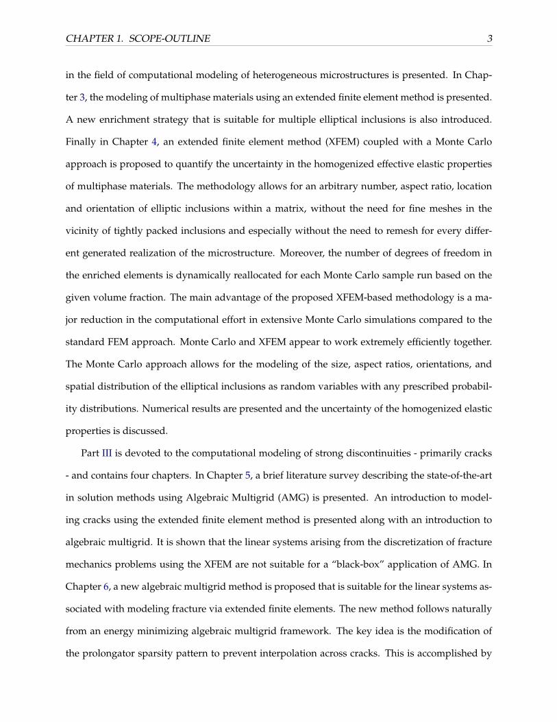
in the field of computational modeling of heterogeneous microstructures is presented. In Chap-
ter 3, the modeling of multiphase materials using an extended finite element method is presented.
A new enrichment strategy that is suitable for multiple elliptical inclusions is also introduced.
Finally in Chapter 4, an extended finite element method (XFEM) coupled with a Monte Carlo
approach is proposed to quantify the uncertainty in the homogenized effective elastic properties
of multiphase materials. The methodology allows for an arbitrary number, aspect ratio, location
and orientation of elliptic inclusions within a matrix, without the need for fine meshes in the
vicinity of tightly packed inclusions and especially without the need to remesh for every differ-
ent generated realization of the microstructure. Moreover, the number of degrees of freedom in
the enriched elements is dynamically reallocated for each Monte Carlo sample run based on the
given volume fraction. The main advantage of the proposed XFEM-based methodology is a ma-
jor reduction in the computational effort in extensive Monte Carlo simulations compared to the
standard FEM approach. Monte Carlo and XFEM appear to work extremely efficiently together.
The Monte Carlo approach allows for the modeling of the size, aspect ratios, orientations, and
spatial distribution of the elliptical inclusions as random variables with any prescribed probabil-
ity distributions. Numerical results are presented and the uncertainty of the homogenized elastic
properties is discussed.
Part III is devoted to the computational modeling of strong discontinuities - primarily cracks
- and contains four chapters. In Chapter 5, a brief literature survey describing the state-of-the-art
in solution methods using Algebraic Multigrid (AMG) is presented. An introduction to model-
ing cracks using the extended finite element method is presented along with an introduction to
algebraic multigrid. It is shown that the linear systems arising from the discretization of fracture
mechanics problems using the XFEM are not suitable for a “black-box” application of AMG. In
Chapter 6, a new algebraic multigrid method is proposed that is suitable for the linear systems as-
sociated with modeling fracture via extended finite elements. The new method follows naturally
from an energy minimizing algebraic multigrid framework. The key idea is the modification of
the prolongator sparsity pattern to prevent interpolation across cracks. This is accomplished by

CHAPTER 1. SCOPE-OUTLINE 4
accessing the standard levelset functions used during the discretization process. Numerical ex-
periments illustrate that the resulting method converges in a fashion that is relatively insensitive
to mesh resolution and to the number of cracks or their location. In Chapter 7, an alternative AMG
approach is used to accelerate the iterative solvers for linear systems arising from XFEM fracture
problems. The methods described in Chapter 6 require several modifications to the AMG to im-
prove convergence. Here the XFEM system itself is transformed into a different representation that
makes it more suitable for a direct application of AMG. It is shown that a transformation exists
to represent the XFEM system in an equivalent phantom node representation that decouples the
graph of the global stiffness matrix across strong discontinuities. Some parallel implementation
aspects and numerical examples are also discussed.
Finally Part IV contains the summary and concluding remarks. A list of the author’s primary
contributions in the field of modeling and solution of solid mechanics problems involving discon-
tinuities is presented. Following this part is the bibliography and the appendices. In Appendix A,
a collaborative work with Luc Berger-Vergiat involving a domain decomposition method for im-
proving the AMG method for XFEM linear systems is described. In Appendix B, another collabo-
rative effort with Eleni Chatzis is described and it involves the use of XFEM coupled with genetic
algorithms for flaw detection in structures. Finally a brief description of the XFEM and AMG
programs developed is provided in Appendix C.

Part II
Weak Discontinuities

CHAPTER 2. STATE-OF-THE-ART 6
Chapter 2
Motivation & Literature Survey
In this chapter, the motivation to study the computational modeling of weak discontinuities is presented. Further a
brief survey of the state-of-the-art in this field is also presented. The inputs from co-authors of the paper (Hiriyur et.
al. [31]) from which the main chapters in this section are reproduced are gratefully acknowledged.
2.1 Motivation & Literature Survey
Composite materials are commonly used in engineering practice as they can be designed to pro-
vide a desired mechanical behavior, while satisfying other requirements such as weight density,
thermal conductivity, durability etc. Fiber-reinforced materials, metal composites, concrete and
ceramics are some of the widely used materials of composite nature. Several examples of complex
multiphase materials including fiber-reinforced ceramic metal composites and carbon nanotubes
are shown in Fig. 2.1. The mechanical behavior of composites is governed by the mechanical
properties of their individual components, their volume fractions and other parameters defining
their spatial and size distribution. In many cases, only the macroscopic mechanical behavior is of
interest, but understanding the microstructure is also extremely important. However, a complete
deterministic analysis of the medium taking the microstructure into account would involve too
much computational effort and may not be feasible. It is therefore necessary to approximate the
complex microstructures with equivalent effective homogeneous material properties.
To obtain the effective homogeneous properties of the composite materials, various methods
have been proposed and used - both analytical [20, 18, 67, 39] and numerical [23, 36, 64, 52, 3, 83].

CHAPTER 2. STATE-OF-THE-ART 7
(a) (b) (c)
Figure 2.1: (a,b) Scanning Electron Microscope micrographs of ceramic matrix composite fromFair et. al. [21] (c) SEM micrograph of carbon nanotubes from Zhang et. al. [85]
Monte Carlo based stochastic homogenization involves the computational analysis of a large num-
ber of randomly generated realizations of the composite medium. The results from these analyses
are then used to derive the effective properties of an equivalent homogeneous medium and quan-
tify their inherent uncertainties. The heterogeneity of composites can have significant variation
across different spatial scales. Consequently, various multi-scale approaches to analyze such ma-
terials have been proposed, along with damage models for particle decohesion [42, 24, 53, 38, 35].
Figure 2.2 shows one such information passing approach applied to the modeling of nanocompos-
ites within the coatings of traditional fiber laminated composites. Information passing or sequen-
tial multiscale methods involves the computation of quantities at the finer scale and then injecting
them on to the coarser scale [22, 66]. Classical finite element methods are commonly used to an-
alyze complex microstructures. In this case, the mesh conforms to the internal material interface
boundaries that cause the strong or weak discontinuities in the displacement solution field. While
fast meshing algorithms are available to discretize a domain with such internal features, this step
still involves a significant computational effort. This is especially true when a large number of
simulations has to be performed along the lines of a Monte Carlo approach reflecting the var-
ious uncertainties involved. Alternatively pixel and voxel based methods have also been used
to analyze complex microstructures by constructing finite elements directly from microstructure
images [57]. By incorporating brute-force techniques, these methods may yield accurate represen-

CHAPTER 2. STATE-OF-THE-ART 8
tations of complex microstructure features. However, these approaches are also computationally
intensive and additionally, the effort involved is proportional to the pixel/voxel resolution, which
should be sufficiently high to capture complexities in the microstructure that it models. Moreover,
the generation of voxel-based elements from sets of 3-dimensional images is not a trivial task and
involves significant complexities.
(a)
Fiber
nanocomposite
(b) (c) (d)
Figure 2.2: Multiscale information-passing approach: (a) composites scale (b) fiber scale (c) coat-ing scale (d) nanotube scale
Development of XFEM [4, 46] has provided a way of dispensing with the need for remeshing
each random realization of the material microstructure in a Monte Carlo formulation. XFEM uses
nodal enrichment functions within the framework of the partition of unity method to augment
the finite element approximations over a structured mesh [44, 60, 9]. These enrichment functions
act as additional bases to model strong or weak discontinuities that are known to occur along
the interface boundaries. References [5, 47] provide exhaustive reviews of the developments in
extended finite element methods to date. While much of the focus of the research community
in this field has been on using this method for numerical modeling of fracture and crack prop-
agation [32, 7], there have also been many papers on the application of XFEM to model weak
discontinuities in solid mechanics problems. For example, the use of level-sets within the frame-
work of XFEM for modeling holes and inclusions has been proposed by Sukumar et al. [63] and
GFEM enrichment functions for discontinuous gradient fields have been studied by Aragon et
al. [1]. Alternate methods similar to XFEM have been proposed to model strong and weak dis-

CHAPTER 2. STATE-OF-THE-ART 9
continuities but using polynomial approximations similar to classical FEM and not modeling the
jump in displacement or strain as explicit variables [27]. More recently the use of XFEM to model
inclusion problems in viscoelastic materials has been explored [84] and extended stochastic finite
element methods for solving stochastic PDEs have been proposed [50].
In previous literature on the use of XFEM for modeling multiphase media, the discrete approx-
imations of the displacement fields were enriched by a single weakly discontinuous function. This
results in the need for high mesh densities in regions where the inclusions are tightly packed. In
the author’s work, the idea is to extend the framework of XFEM to incorporate the enrichments
of multiple weakly discontinuous functions over a single element domain. The scalar coefficients
corresponding to these multiple enrichment functions then act as unknown virtual degrees of
freedom added on to the global system of equations. The number of these additional degrees of
freedom associated with a particular node is also a variable that depends on the number of inclu-
sions enriching the elements containing the node. A similar approach of using multiple level sets
to prevent numerical artefacts arising from nearby inclusions in XFEM has been proposed by Tran
et al. [68]. To quantify the uncertainty in the homogenized effective properties of these multiphase
materials, the model is coupled with a Monte Carlo simulation approach, where a large number of
random realizations of the microstructure are analyzed. Therefore the probability distributions of
the size, aspect ratio, orientation and spatial distribution of the elliptical inclusions considered in
this work can be readily incorporated into the analysis of the output uncertainties. The following
chapters in this section are organized as follows: In section 3.1, the XFEM equations to model ellip-
tical inclusions are developed and the framework extended to include multiple inclusions within
an element domain. A comparison of the XFEM implementation with results obtained from a
benchmark FEM solution is also presented. In section 4.1, a description is provided for the Monte
Carlo simulation approach that is used to obtain the probability distribution of the output effec-
tive properties while modeling the randomness in the input microstructure. Finally the approach
used for finding the effective elastic properties of the homogenized microstructure is described in
section 4.2. The proposed approach is applied in three cases: stiff circular inclusions, stiff elliptical

CHAPTER 2. STATE-OF-THE-ART 10
inclusions and finally soft elliptical inclusions.

CHAPTER 3. XFEM-INCLUSIONS 11
Chapter 3
Modeling Inclusions via XFEM
In this chapter, an introduction to the extended finite element method in the context of modeling weak discontinuities
such as inclusions and material inhomogeneities is presented. A simple enrichment formulation suitable for elliptical
inclusions is presented. The traditional XFEM approach to modeling inclusions is extended to accommodate multiple
phase-separations within a single element domain.
3.1 XFEM for Weak Discontinuities
3.1.1 Fundamental equations
The discrete approximation for the displacement field within an element as used in classical FEM
is given in Eq. (3.1):
uh(x) =nen
∑j=1
Nj(x)uj (3.1)
where nen represents the number of element nodes and the nodal shape functions satisfy the
partition of unity condition described as ∑∀I
NI(x) = 1, ∀x ∈ Ωe .
An element that contains inclusions with discontinuous material properties within its bound-
aries will have a weakly discontinuous displacement field along the interface boundaries. Clearly,
the nodal shape functions Nj, which form a set of smooth and continuous functions are by them-
selves inadequate to model this weakly discontinuous displacement field. In XFEM, the basis
functions are “enriched” through a function ϕ(x) that satisfies the local character of the displace-
ment field that the discrete approximation aims to model. A description of the enrichment func-

CHAPTER 3. XFEM-INCLUSIONS 12
tion ϕ(x) that has been developed for an arbitrarily oriented elliptical inclusion is provided in
section 3.1.2. To satisfy partition of unity, the enrichment function is enveloped by the original
shape functions Nj and corresponding additional scalar nodal coefficients aj introduced in the
equation. This leads to the XFEM discrete approximation for an element containing a single ma-
terial inclusion:
uh(x) =nen
∑j=1
Nj[uj + ϕ(x)aj
](3.2)
When multiple inclusions are closely packed together as shown in Fig. 3.1, the mesh density
Figure 3.1: Multiple inclusions within element boundary
would have to be quite large so that the enrichment functions corresponding to the different inclu-
sions do not interfere. To overcome this limitation, the formulation is further extended to include
multiple enrichment functions as described in Eq. (3.3). Here, we have enrichment functions ϕi
corresponding to each inclusion i within the element domain that add to the set of basis functions
in modeling the displacement field. The additional scalar nodal coefficients ajk corresponding to
these functions are unknowns to be found, and act as virtual degrees of freedom in the global
CHAPTER 3. XFEM-INCLUSIONS 13
system of equations:
uh(x) =nen
∑j=1
Nj(x)uj +nen
∑j=1
Nj(x)
inclusion 1︷ ︸︸ ︷φj1(x)aj1 +
inclusion 2︷ ︸︸ ︷φj2(x)aj2 + · · ·+
inclusion n0︷ ︸︸ ︷φjn0(x)ajn0
=
nen
∑j=1
Nj(x)
[uj +
n0
∑k=1
φjk(x)ajk
](3.3)
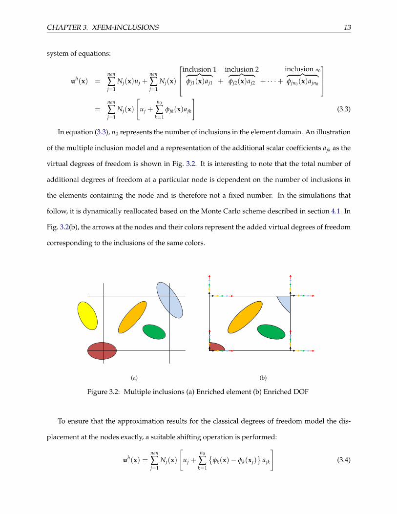
In equation (3.3), n0 represents the number of inclusions in the element domain. An illustration
of the multiple inclusion model and a representation of the additional scalar coefficients ajk as the
virtual degrees of freedom is shown in Fig. 3.2. It is interesting to note that the total number of
additional degrees of freedom at a particular node is dependent on the number of inclusions in
the elements containing the node and is therefore not a fixed number. In the simulations that
follow, it is dynamically reallocated based on the Monte Carlo scheme described in section 4.1. In
Fig. 3.2(b), the arrows at the nodes and their colors represent the added virtual degrees of freedom
corresponding to the inclusions of the same colors.
(a)
(b)
Figure 3.2: Multiple inclusions (a) Enriched element (b) Enriched DOF
To ensure that the approximation results for the classical degrees of freedom model the dis-
placement at the nodes exactly, a suitable shifting operation is performed:
uh(x) =nen
∑j=1
Nj(x)
[uj +
n0
∑k=1
φk(x)− φk(xj)
ajk
](3.4)

CHAPTER 3. XFEM-INCLUSIONS 14
The strain field is related to the displacement field through the gradients of the basis functions
B(x) as shown in Eq. (3.5):
ε(x) = B(x) · u (3.5)
In the case of XFEM representation of the displacement field, the gradients of the enrichment
functions also influence the strain field. Thus the expression for the strain ε at any point x along
the direction xi is written as in Eq. (3.6):
ε i(x) =nen
∑j=1
Bij(x)
[uj +
n0
∑k=1
ϕ(x)− ϕ(xj)
ajk
]+
nen
∑j=1
Nj(x)
[uj +
n0
∑k=1
∂’k(x)∂xi
ajk
](3.6)
=⇒ B =
[BFEM BENR
1 BENR2 · · · BENR
n0
](3.7)
Here, the B matrix in the XFEM approximation can be seen as consisting of two parts - the classical
FEM part which corresponds to the nodal displacement degrees of freedom uj and the augmented
virtual part which corresponds to the enriched degrees of freedom ajk. The size of the augmented
virtual part is dependent on the number of inclusions enriching the corresponding element nodes.
In the stochastic homogenization approach, this number is a random variable and depends on the
parameters describing the size and spatial distribution of inclusions. Using this B matrix and the
constitutive equations, the stiffness terms can be computed from numerical integration as shown
in equations (3.8) and (3.9). In these equations, ngp refers to the number of quadrature points
and wi are the corresponding weights. The numerical quadrature may be performed by either
partitioning the element domain into sub-triangles/sub-quads and using Gauss points with ap-
propriate weights or by using a large number of equidistant trapezoidal integration points along
each spatial dimension. Recently, an alternative approach to integrating strong and weak dis-
continuities in XFEM without using integration subcells has been proposed [49]. The trapezoidal
integration method with 64 quadrature points in an equispaced 8× 8 grid is used in the current
CHAPTER 3. XFEM-INCLUSIONS 15
work:
Keij =
∫Ωe
BiDBjdΩe (3.8)
=ngp
∑k=1
wiBi(xk)D(xk)Bj(xk) (3.9)
where D represents the material constitutive matrix.
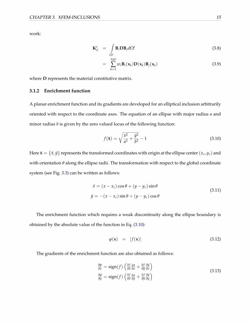
3.1.2 Enrichment function
A planar enrichment function and its gradients are developed for an elliptical inclusion arbitrarily
oriented with respect to the coordinate axes. The equation of an ellipse with major radius a and
minor radius b is given by the zero valued locus of the following function:
f (x) =
√x2
a2 +y2
b2 − 1 (3.10)
Here x = x, y represents the transformed coordinates with origin at the ellipse center (xc, yc) and
with orientation θ along the ellipse radii. The transformation with respect to the global coordinate
system (see Fig. 3.3) can be written as follows:
x = (x− xc) cos θ + (y− yc) sin θ
y = −(x− xc) sin θ + (y− yc) cos θ
(3.11)
The enrichment function which requires a weak discontinuity along the ellipse boundary is
obtained by the absolute value of the function in Eq. (3.10):
ϕ(x) = | f (x)| (3.12)
The gradients of the enrichment function are also obtained as follows:
∂φ∂x = sign( f )
(∂ f∂x
∂x∂x + ∂ f
∂y∂y∂x
)∂φ∂y = sign( f )
(∂ f∂x
∂x∂y + ∂ f
∂y∂y∂y
) (3.13)

CHAPTER 3. XFEM-INCLUSIONS 16
𝑥𝑥
𝑦𝑦
𝑥 𝑦𝑦
(𝑥𝑥𝑐𝑐 ,𝑦𝑦𝑐𝑐)
𝜃𝜃
Figure 3.3: The two coordinate systems
Where the gradient functions with respect to the transformed coordinates are given as follows:
∂ fdx = x
a2
(√x2
a2 +y2
b2
)−1
∂ fdy = y
b2
(√x2
a2 +y2
b2
)−1 (3.14)
The final form of the gradients of the enrichment function are obtained by plugging (3.14) in
(3.13):∂ϕ∂x = sign( f )
(√x2
a2 +y2
b2
)−1 (x cos(θ)
a2 − y sin(θ)b2
)∂ϕ∂y = sign( f )
(√x2
a2 +y2
b2
)−1 (x sin(θ)
a2 + y cos(θ)b2
) (3.15)
A graphical description of the enrichment function and its gradients is provided in Fig. 3.4.
3.1.3 Convergence study of XFEM solution for single inclusion
A convergence study is performed to compare the XFEM solution developed using the enrich-
ment function described in section 3.1.2 against a standard FEM solution. In the latter case, an
FEM mesh conforming to the interface boundaries is formed using quadrilateral bilinear elements.
These quadrilateral meshes are obtained using a python script within ABAQUS. A unit cell of size
1× 1 is subject to the boundary and loading configuration shown in Fig. 3.5. The magnitude of the
edge traction along the right edge is 1E3. The matrix and the inclusion are modeled using linear

CHAPTER 3. XFEM-INCLUSIONS 17
(a)
0.20.2
0.2
0.2
0.2
0.2
0.2
0.2
0.2
0.2
0.2
0.2
0.4
0.4
0.4
0.4
0.4
0.4
0.4
0.4 0.
4
0.4
0.4
0.4
0.6
0.6
0.6
0.6
0.6
0.6
0.6
0.6
0.6
0.6
0.60.8
0.8
0.8
0.8
0.8
1
1
1
1
1.2
1.2
1.4
1.4
1.6
1.6
−1 −0.8 −0.6 −0.4 −0.2 0 0.2 0.4 0.6 0.8 1−1
−0.8
−0.6
−0.4
−0.2
0
0.2
0.4
0.6
0.8
1
(b)
(c) (d)
Figure 3.4: Enrichment function for an elliptical inclusion within an element: (a) ϕ(x), (b) Contourlevels of ϕ(x), (c) ∂ϕ
∂x , (d) ∂ϕ∂y

CHAPTER 3. XFEM-INCLUSIONS 18
isotropic materials with the following elastic properties:
Matrix : Em = 70 · 103 MPa
Inclusions : Ep = 410 · 103 MPa(3.16)
Poisson’s ratio for both the matrix and the inclusion is set equal to 0.3. To obtain the stiffness
quantities in XFEM, the numerical integration in Eq. (3.8) is performed in the element domain
using 8× 8 equispaced quadrature points. The following variable parameters are considered in
this study: the inclusion aspect ratio (0.2, 0.4 0.6, 0.8 and 1) and the orientation angle (0, 45, 90)
with respect to the loading direction. Figure 3.6 shows the meshes and the displacement solutions
obtained using XFEM and FEM for the case of the inclusion ellipse aspect ratio being equal to
0.4 and the orientation angle of the major axis being equal to 45 with respect to the global x
axis. Agreement between FEM and XFEM solutions is excellent. Similar quality of agreement was
observed for all the cases considered involving the aforementioned values for the aspect ratio and
the orientation angle.
𝑥𝑥
𝑦𝑦
Figure 3.5: Schematic of load and boundary conditions
The differences in the solutions obtained from XFEM and FEM analyses are plotted against
the logarithm of the XFEM element size in Fig. 3.7 for five different aspect ratios r. The plots in
the left column show the relative norm of the difference in displacement solutions and the plots

CHAPTER 3. XFEM-INCLUSIONS 19
in the right column show the difference in strain energies computed by XFEM and FEM. The
results indicate that when the orientation of the elliptical inclusion is parallel or perpendicular
to the loading direction (θ = 0 or 90 degrees), the convergence rates for all the ellipse aspect
ratios considered are very close to each other. When the orientation of the elliptical inclusion is
45 degrees, the difference in the convergence rates for the different aspect ratios vary slightly; the
convergence being slowest when the aspect ratio is 0.2.
(a) (b)
(c) (d)
Figure 3.6: Displacement solution comparison (a) XFEM mesh (b) XFEM displacements (c) FEMmesh (d) FEM displacements
Since the enrichment function described in section 3.1.2 is designed for approximation of

CHAPTER 3. XFEM-INCLUSIONS 20
−1.5 −1 −0.5 0
−3
−2
−1
0
θ = 0
−1.5 −1 −0.5 0
−3
−2
−1
0
θ = 45
ln(||(u
fem
−uxfem)||
2/||
ufem|| 2)
11
2
1
−1.5 −1 −0.5 0
−3
−2
−1
0
θ = 90
Size of XFEM element: ln(h)
−1.5 −1 −0.5 0
−6
−5
−4
−3
θ = 0
−1.5 −1 −0.5 0
−6
−5
−4
−3
θ = 45ln(||(Π
fem
−Π
xfem)||
2/||
Πfem|| 2)
−1.5 −1 −0.5 0
−6
−5
−4
−3
θ = 90
Size of XFEM element: ln(h)
r = 0.2
r = 0.4
r = 0.6
r = 0.8
r = 1
Figure 3.7: Convergence of XFEM results to FEM results

CHAPTER 3. XFEM-INCLUSIONS 21
weakly discontinuous C0 fields, it is ideally suited when the difference in elastic moduli between
the matrix and inclusions is relatively small. Some studies have shown that an XFEM formulation
using an enrichment function that is based on a discontinuous deformation map is better suited
when there is a large modulus mismatch [62]. To study the effect of the ratio of the elastic moduli
of the two phases on the convergence properties of the XFEM enrichment function described in
section 3.1.2 towards a reference benchmark solution, the following test is performed. A unit cell
of size 1× 1 with a single elliptical inclusion (of aspect ratio r = 0.5 and orientation angle θ = 45)
is subjected to the same boundary conditions and loading as described earlier in this section. In
this study, only the ratio of the elastic moduli of the two phases is varied (Em is fixed at 70 · 103MPa
and the ratio Ep/Em is varied from 2 to 1,000 for stiff inclusions and from 0.001 to 0.5 for soft inclu-
sions) keeping all other parameters unchanged. XFEM analyses and reference FEM analyses are
performed for each ratio of the moduli and the two solutions are compared. In Fig. 3.8, the relative
differences (in terms of strain energy and displacements) of the two solutions are plotted against
the corresponding ratio of the elastic moduli. It is observed that the XFEM solution is increasingly
diverging from the reference FEM solution as the moduli ratio increases. The divergence appears
to be larger for the case of stiff inclusions. However, even for the largest ratio considered (1,000),
the difference in the two solutions is only about 1.4%. For the moduli ratios considered in the
convergence studies (refer to sections 3.1.3 and 3.1.4) and the Monte Carlo simulations (refer to
section 4.2.1), the differences between XFEM and the reference FEM solution are at most 0.3%.
3.1.4 Convergence study of XFEM solution for multiple inclusions
Implementation of the proposed XFEM approach for multiple inclusions is performed in MAT-
LAB. For the benchmark verification study between XFEM and FEM, a specific realization involv-
ing 15 elliptical inclusions of volume fraction 0.3, uniformly scattered in a 2D unit cell is studied.
The test configuration (size of the unit cell, material properties of the two phases, boundary condi-
tions and loads) is identical to the description provided in the preceding section. Figure 3.9 shows
the mesh discretization used for the reference FEM study and a representative XFEM discretiza-

CHAPTER 3. XFEM-INCLUSIONS 22
100
101
102
103
0
0.002
0.004
0.006
0.008
0.01
0.012
0.014
|Πxfem−Π
fem|/Π
fem
Ep > Em
Em > Ep
100
101
102
103
0
0.001
0.002
0.003
0.004
0.005
0.006
0.007
||uxfem−ufem|| 2/||ufem|| 2
Ratio of Elastic Moduli
E−ratio used in this paper
E−ratio used in this paper
Figure 3.8: Effect of elastic moduli ratio on accuracy of XFEM solution
tion (among the many considered for this convergence study). The benchmark FEM analysis was
performed using a quadrilateral mesh containing 12,842 nodes and 12,641 elements (shown in
Fig. 3.9a). The XFEM analyses were performed using structured square meshes of sizes ranging
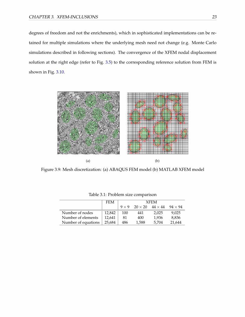
from 9× 9 elements to 94× 94 elements. Table 3.1 shows the comparison of the problem sizes
(nodes, elements and degrees of freedom) for the different discretizations considered. The XFEM
analyses involved the solution of smaller systems of equations compared to the corresponding
reference FEM mesh. However, it must be noted that in XFEM case, the establishment of the ele-
ment stiffness matrices involves a larger effort compared to FEM since more quadrature points are
required to accurately integrate over a weakly discontinuous field. This drawback however is off-
set by the benefits of having far simpler structured mesh generation and solving a smaller global
system of equations. As the mesh is refined, the number of global system of equations (unknown
degrees of freedom) in XFEM is approaching the size of the benchmark FEM system. However,
a majority of these degrees of freedom correspond to nodal displacements (i.e., the regular FEM
CHAPTER 3. XFEM-INCLUSIONS 23
degrees of freedom and not the enrichments), which in sophisticated implementations can be re-
tained for multiple simulations where the underlying mesh need not change (e.g. Monte Carlo
simulations described in following sections). The convergence of the XFEM nodal displacement
solution at the right edge (refer to Fig. 3.5) to the corresponding reference solution from FEM is
shown in Fig. 3.10.
(a) (b)
Figure 3.9: Mesh discretization: (a) ABAQUS FEM model (b) MATLAB XFEM model
Table 3.1: Problem size comparison
FEM XFEM9× 9 20× 20 44× 44 94× 94
Number of nodes 12,842 100 441 2,025 9,025Number of elements 12,641 81 400 1,936 8,836Number of equations 25,684 486 1,588 5,704 21,644

CHAPTER 3. XFEM-INCLUSIONS 24
0 .2 .4 .6 .8 10.008
0.009
0.01
0.011
0.012
y-coordinate along right edge
x-displacemen
talon
grigh
ted
ge
FEM 12641 elems
XFEM 9×9
XFEM 20×20
XFEM 44×44
XFEM 94×94
(a)
−3 −2 −1 0−5
−4
−3
−2
Size of XFEM element: ln(h)
ln(||(u
fem
−uxfem)||
2/||
/ufem|| 2)
1
1
(b)
Figure 3.10: Convergence of XFEM results to benchmark FEM results for the case of multipleinclusions: (a) Convergence of x displacements along right edge (b) Relative norm of the differencein edge displacements versus XFEM element size

CHAPTER 4. XFEM-MC 25
Chapter 4
Homogenization of RandomMicrostructures
In this chapter, the extended finite element method is coupled with the Monte-Carlo approach to be used in
uncertainty quantification in homogenization of random heterogeneous microstructures.
4.1 Monte Carlo approach
The first step of the proposed Monte Carlo based stochastic homogenization involves the gener-
ation of a large number of random realizations of the microstructure geometry based on a given
volume fraction of the inclusions and other parameters representing the uncertainties in their
number, aspect ratios, spatial distribution and orientation. There are several methods available
for this purpose, an example being the random growth algorithm [40]. The approach used in this
work (with certain similarities to the ballistic deposition algorithm [79]) is described in section
4.1.1. Once the random microstructures are obtained, deterministic elastic analyses are performed
for a unit cell containing these generated microstructures, when subjected to a predetermined set
of loads and boundary conditions. Finally, the effective homogeneous properties corresponding
to these random microstructures are obtained by finding the best-fit material properties for an
equivalent homogeneous unit cell subjected to the same loads and boundary conditions. When
XFEM is used, the equivalent homogeneous unit cell is obtained from the same mesh with the
internal boundaries and enrichments removed. Through the residual minimization routine, uni-
form material properties are assigned at all the quadrature points. The discrete problem for the
CHAPTER 4. XFEM-MC 26
homogeneous medium then reduces to a classical FEM one and the solution is obtained at the
same nodal points as the heterogeneous case.
A strain energy approach is used in this work to determine the homogenized effective prop-
erties. For the case considered here involving a linear isotropic material under plane stress con-
ditions, there are two independent effective properties to be found: the elastic modulus Ee f f and
Poisson’s ratio νe f f . To obtain the best-fit estimates for these two quantities, an optimization algo-
rithm is used with a residual quantity R as the objective function to be minimized and the material
properties as the control variables. As shown in Eq. (4.1), the residual quantity R is defined in
terms of the difference in internal strain energy stored in the heterogeneous system (computed us-
ing XFEM including enrichments) and the corresponding homogenized systems (computed using
classical FEM without enrichments):
RU(E, ν, · · · ) ≡⟨∫
Ω
σ : εdΩ
⟩XFEM
−⟨∫
Ω
σ : εdΩ
⟩FEM
(4.1)
The most important benefit of XFEM is realized when performing the elastic analyses of the
multiple randomly heterogeneous microstructures on a fixed structured mesh. Only the enrich-
ments and the corresponding additional degrees of freedom change in each Monte Carlo simu-
lation, thereby avoiding the need to remesh every generated random microstructure. An added
benefit of using XFEM is that it allows for easy comparison of individual nodal and elemental
solution quantities across different random realizations of the microstructure and equivalent ho-
mogeneous systems as the mesh remains the same. A similar type of optimization using XFEM
has been proposed for adapting the enrichment function to the solution [76] and for detection of
flaws in structures [54, 77].
4.1.1 Random microstructure generation
The Monte Carlo procedure to generate a large number of sample realizations of a unit cell of the
microstructure is described in Algorithm 4.1.1. The inclusions are described through the volume
fraction λ, the total number of inclusions np within the unit cell and independent probability

CHAPTER 4. XFEM-MC 27
distributions for the following: inclusion relative major radius f a, aspect ratio fr, location of the
ellipse center fc and ellipse orientation fθ . The first step is to generate the elliptical inclusions. To
this end, values representing the relative inclusion major radius ai and the inclusion aspect ratio ri
are generated according to prescribed PDF’s (assumed independent). The subscript i ranges from
1 to np. The minor radii are calculated as bi = ri ai. The inclusion sizes obtained are relative to the
prescribed distributions and need to be scaled to represent the prescribed volume fraction λ. The
cumulative area of all the randomly generated inclusions is then computed and an appropriate
scaling factor is determined and applied to the major and minor radii to obtain the final inclusion
sizes reflecting the prescribed volume fraction. It should be mentioned that the scaled inclusion
major radii ai do not follow strictly the prescribed PDF f a. Its shape is preserved but not its mean
value and variance.
The next step is to spatially distribute the generated inclusions within the base matrix repre-
senting the unit cell, starting with the largest inclusion and following with the remaining inclu-
sions in decreasing order of size. Values representing the coordinates of the ellipses’ centers and
their orientations are generated according to the prescribed probability distributions ( fc and fθ
respectively). If an inclusion centered at such generated coordinates is found to overlap with any
other previously generated and spatially placed inclusion(s), new center coordinates and orien-
tation are generated until no overlap is observed. The procedure continues then with the next
smaller inclusion. By spatially distributing the inclusions in decreasing order of size, the prob-
ability of overlap of a particular inclusion with others that have been previously placed within
the unit cell is reduced. A set of sample realizations obtained using Algorithm 4.1.1 for different
volume fractions λ and number of inclusions np is shown in Fig. 4.1.
4.2 Homogenization
4.2.1 Application and results
The proposed framework of using XFEM coupled with Monte Carlo simulations is used to obtain
the probability distribution of the effective elastic modulus for a plane-stress medium containing

CHAPTER 4. XFEM-MC 28
=
0.1
=
0.2
=
0.3
=
0.4
=
0.5
np = 1 n
p = 10 n
p = 20 n
p = 30
Figure 4.1: Sample realizations of generated random microstructures

CHAPTER 4. XFEM-MC 29
Algorithm 4.1.1 Random Microstructure Generation
• INPUT
– X1, X2: Size of the unit cell
– λ: Inclusion volume fraction
– np: Total number of inclusions in unit cell
– f a, fr, fc, fθ: Independant probability distributions for the relative major
radius, aspect ratio, center coordinates and orientation angle
• GENERATE/SCALE/SORT INCLUSIONS
– Generate np random numbers to represent relative major radius aifollowing the prescribed probability distribution f a
– Generate np random numbers to represent the aspect ratio ri following the
prescribed probability distribution fr
– Obtain the relative minor radii bi = ri ai and cumulative area Aincl =
πnp
∑k=1
ai bi
– Scale radii: ai = ai
√λ · X1X2
Aincland bi = bi
√λ · X1X2
Aincl
– Sort inclusions in decreasing order of size
• SPATIALLY DISTRIBUTE ON UNIT CELL
– Loop over inclusions k = 1 to np
∗ Generate random numbers xk, yk (uniform in [0, X1] and [0, X2]respectively) and θk (uniform in [0, 2π]) to represent inclusion
ellipse center and orientation
∗ Check overlap with previously positioned inclusions 1 to k· If TRUE, repeat step for inclusion k with new random values for
coordinates xk, yk and orientation θk
· if FALSE, proceed to next smaller inclusion
elliptical inclusions. A linear isotropic material model is used for the matrix and the inclusion
phases and for simplicity, the homogenization is assumed to preserve this property. Therefore
only two independent effective material properties are computed: effective elastic modulus Ee f f
and effective Poisson’s ratio νe f f . It should be noted that a more general orthotropic model would
be more accurate for the resulting homogenized medium. However using such a model involves
a significantly higher computational cost and therefore it is not used in the current study as it
CHAPTER 4. XFEM-MC 30
is not contributing towards the main objectives of this work. Here, the effective Poisson’s ratio
is fixed a priori to the common Poisson’s ratio for the two phases (νm = νp = 0.3 → νe f f ) and
the residual RU in Eq. (4.1) is minimized with respect to the effective elastic modulus Ee f f alone.
In the examples provided here, the size of the domain is smaller than the typical representative
volume element and therefore a strict comparison to the homognized effective properties would
not be accurate. However for comparison and perspective, the following three models for effective
elastic properties are provided:
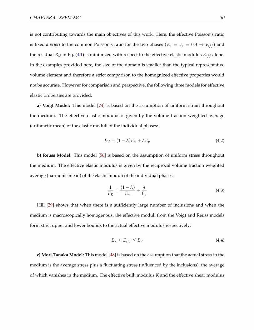
a) Voigt Model: This model [74] is based on the assumption of uniform strain throughout
the medium. The effective elastic modulus is given by the volume fraction weighted average
(arithmetic mean) of the elastic moduli of the individual phases:
EV = (1− λ)Em + λEp (4.2)
b) Reuss Model: This model [56] is based on the assumption of uniform stress throughout
the medium. The effective elastic modulus is given by the reciprocal volume fraction weighted
average (harmonic mean) of the elastic moduli of the individual phases:
1ER
=(1− λ)
Em+
λ
Ep(4.3)
Hill [29] shows that when there is a sufficiently large number of inclusions and when the
medium is macroscopically homogenous, the effective moduli from the Voigt and Reuss models
form strict upper and lower bounds to the actual effective modulus respectively:
ER ≤ Ee f f ≤ EV (4.4)
c) Mori-Tanaka Model: This model [48] is based on the assumption that the actual stress in the
medium is the average stress plus a fluctuating stress (influenced by the inclusions), the average
of which vanishes in the medium. The effective bulk modulus K and the effective shear modulus

CHAPTER 4. XFEM-MC 31
G are obtained as follows:
K = Km +λKm(Kp − Km)
Km + β2(1− λ)(Kp − Km)
G = Gm +λGm(Gp − Gm)
Gm + β1(1− λ)(Gp − Gm)
where β1 = 2(4−5νm)15(1−νm)
and β2 = 3− 5β1. The effective elastic modulus is then given as follows:
EMT =9KG
3K + G(4.5)
In the Monte Carlo simulations that follow, three different cases are considered: (a) stiff circu-
lar inclusions, (b) stiff elliptical inclusions and (c) soft elliptical inclusions. A total of 2000 Monte
Carlo simulations are performed for each volume fraction λ considered ranging from 0.1 to 0.5.
The number of inclusions np varies from 1 to 30. A unit cell of size 1× 1 subjected to the boundary
conditions shown in Fig. 4.2 is used for this study. The enforced uniform displacements (compres-
sive) on the top and bottom edges are 0.3 times the uniform displacements enforced on the left
and right edges (tensile).
E
Em m
E p p
Figure 4.2: Boundary Conditions (arrows here indicate enforced displacements)

CHAPTER 4. XFEM-MC 32
4.2.1.1 Case 1 - Stiff circular inclusions:
The elastic modulus of the inclusions Ep is related to that of the matrix Em as follows: Ep/Em = 5.8
(the values of Ep and Em mentioned in section 3.1.3 are used). The relative radii of the circular
inclusions follow a uniform distribution in [0.5, 1]. Figure 4.3(a) displays the results of the Monte
Carlo simulations regarding the variation of the effective modulus in terms of the volume fraction
λ. Figure 4.3(b) displays the corresponding histograms of Ee f f for the five values of λ considered.
And the variation of Ee f f with respect to the number of inclusions np is provided in Fig. 4.3(c). The
resulting mean, standard deviation and coefficient of variation of Ee f f for each volume fraction λ
considered are presented in Table 4.1. Figure 4.4 shows the convergence of the mean and COV of
Ee f f with increasing number of Monte Carlo realizations.
Table 4.1: Stiff circular inclusions: Statistics of Ee f f
λ Mean Std. Devn. COV0.1 7.85E+04 5.62E+02 0.00720.2 8.99E+04 1.13E+03 0.01260.3 1.04E+05 2.01E+03 0.01940.4 1.22E+05 2.64E+03 0.02170.5 1.44E+05 3.08E+03 0.0214
4.2.1.2 Case 2 - Stiff elliptical inclusions:
As in the previous case, the elastic modulus of the inclusions Ep is related to that of the matrix
Em as follows: Ep/Em = 5.8 (the values of Ep and Em mentioned in section 3.1.3 are used). The
relative major radii ai of the inclusions follow a uniform distribution in [0.5, 1] and the ellipses’
aspect ratios ri follow a uniform distribution also in [0.5, 1]. Figure 4.5(a) displays the results of the
Monte Carlo simulations regarding the variation of the effective modulus in terms of the volume
fraction λ. Figure 4.5(b) displays the corresponding histograms of Ee f f for the five values of λ
considered. And the variation of Ee f f with respect to the number of inclusions np is provided in
Fig. 4.5(c). The resulting mean, standard deviation and coefficient of variation of Ee f f for each
volume fraction λ considered are presented in Table 4.2. Figure 4.6 shows the convergence of the

CHAPTER 4. XFEM-MC 33
mean and COV of Ee f f with increasing number of Monte Carlo realizations.
Table 4.2: Stiff elliptical inclusions: Statistics of Ee f f
λ Mean Std. Devn. COV0.1 7.84E+04 6.10E+02 0.00780.2 9.00E+04 1.21E+03 0.01350.3 1.04E+05 2.15E+03 0.02060.4 1.22E+05 3.35E+03 0.02750.5 1.44E+05 3.97E+03 0.0275
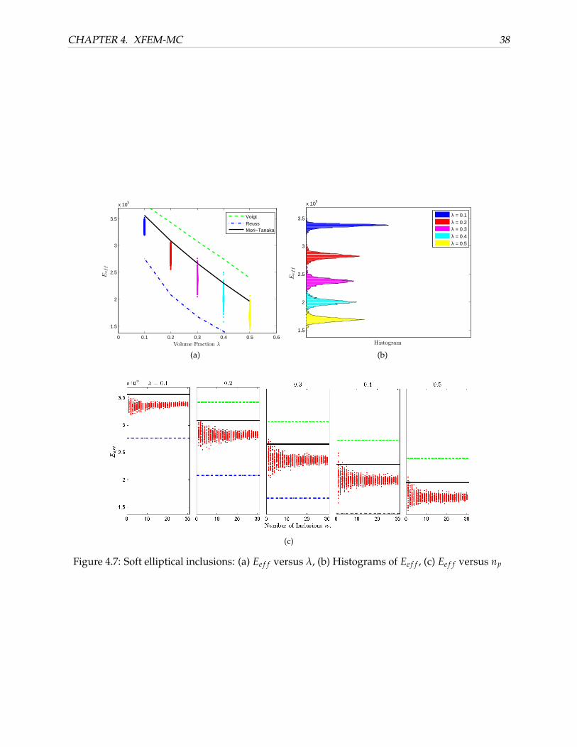
4.2.1.3 Case 3 - Soft elliptical inclusions:
In the third case, the elastic modulus of the matrix is higher than that of the inclusions as: Em/Ep =
5.8 (Ep = 70 · 103 MPa and Em = 410 · 103 MPa). The relative major radii ai of the inclusions follow
a uniform distribution in [0.5, 1] and the ellipses’ aspect ratios ri follow a uniform distribution
also in [0.5, 1]. Figure 4.7(a) displays the results of the Monte Carlo simulations regarding the
variation of the effective modulus in terms of the volume fraction λ. Figure 4.7(b) displays the
corresponding histograms of Ee f f for the five values of λ considered. And the variation of Ee f f
with respect to the number of inclusions np is provided in Fig. 4.7(c). The resulting mean, standard
deviation and coefficient of variation of Ee f f for each volume fraction λ considered are presented
in Table 4.3. Figure 4.8 shows the convergence of the mean and COV of Ee f f with increasing
number of Monte Carlo realizations.
Table 4.3: Soft elliptical inclusions: Statistics of Ee f f
λ Mean Std. Devn. COV0.1 3.37E+05 3.32E+03 0.00990.2 2.82E+05 5.39E+03 0.01910.3 2.37E+05 6.74E+03 0.02840.4 2.00E+05 6.71E+03 0.03360.5 1.69E+05 5.77E+03 0.0342

CHAPTER 4. XFEM-MC 34
0 0.1 0.2 0.3 0.4 0.5 0.6
0.8
0.9
1
1.1
1.2
1.3
1.4
1.5
1.6
x 105
Eeff
Volume Fraction λ
VoigtReussMori−Tanaka
(a)
0.8
0.9
1
1.1
1.2
1.3
1.4
1.5
1.6
x 105
Eeff
Histogram
λ = 0.1λ = 0.2λ = 0.3λ = 0.4λ = 0.5
(b)
(c)
Figure 4.3: Stiff circular inclusions: (a) Ee f f versus λ, (b) Histograms of Ee f f , (c) Ee f f versus np

CHAPTER 4. XFEM-MC 35
050
010
0015
0020
0025
000.
6
0.81
1.2
1.4
1.6
x 10
5
number
ofMonte
Carlosamplesn
µnE=mean(Eeff(1:n))
050
010
0015
0020
0025
000
0.01
0.02
0.03
0.04
number
ofMonte
Carlosamplesn
COV(Eeff(1:n))
λ=
0.1
λ=0.
2
λ=0.
3
λ=0.
4
λ=0.
5
Figu
re4.
4:St
iffci
rcul
arin
clus
ions
:Con
verg
ence
ofM
ean
and
CO
Vof
E eff

CHAPTER 4. XFEM-MC 36
0 0.1 0.2 0.3 0.4 0.5 0.6
0.8
0.9
1
1.1
1.2
1.3
1.4
1.5
1.6
1.7
1.8
x 105
Eeff
Volume Fraction λ
VoigtReussMori−Tanaka
(a)
0.8
0.9
1
1.1
1.2
1.3
1.4
1.5
1.6
1.7
1.8
x 105
Eeff
Histogram
λ = 0.1λ = 0.2λ = 0.3λ = 0.4λ = 0.5
(b)
(c)
Figure 4.5: Stiff elliptical inclusions: (a) Ee f f versus λ, (b) Histograms of Ee f f , (c) Ee f f versus np

CHAPTER 4. XFEM-MC 37
050
010
0015
0020
0025
000.
6
0.81
1.2
1.4
1.6
1.8
x 10
5
number
ofMonte
Carlosamplesn
µnE=mean(Eeff(1:n))
050
010
0015
0020
0025
000
0.02
0.04
0.06
0.08
number
ofMonte
Carlosamplesn
COV(Eeff(1:n))
λ=
0.1
λ=0.
2
λ=0.
3
λ=0.
4
λ=0.
5
Figu
re4.
6:St
iffel
lipti
cali
nclu
sion
s:C
onve
rgen
ceof
Mea
nan
dC
OV
ofE e
ff
CHAPTER 4. XFEM-MC 38
0 0.1 0.2 0.3 0.4 0.5 0.6
1.5
2
2.5
3
3.5
x 105
Eeff
Volume Fraction λ
VoigtReussMori−Tanaka
(a)
1.5
2
2.5
3
3.5
x 105
Eeff
Histogram
λ = 0.1λ = 0.2λ = 0.3λ = 0.4λ = 0.5
(b)
(c)
Figure 4.7: Soft elliptical inclusions: (a) Ee f f versus λ, (b) Histograms of Ee f f , (c) Ee f f versus np

CHAPTER 4. XFEM-MC 39
050
010
0015
0020
0025
001.
52
2.53
3.5
x 10
5
number
ofMonte
Carlosamplesn
µnE=mean(Eeff(1:n))
050
010
0015
0020
0025
000
0.01
0.02
0.03
0.04
0.05
0.06
number
ofMonte
Carlosamplesn
COV(Eeff(1:n))
λ=
0.1
λ=0.
2
λ=0.
3
λ=0.
4
λ=0.
5
Figu
re4.
8:So
ftel
lipti
cali
nclu
sion
s:C
onve
rgen
ceof
Mea
nan
dC
OV
ofE e
ff

CHAPTER 4. XFEM-MC 40
4.2.2 Discussion
In all three cases examined, the uncertainty in the effective elastic modulus Ee f f (indicated by the
spreading of the histograms and the COV values) is increasing as the volume fraction λ increases.
For all three cases too, the general trend is that the coefficient of variation of Ee f f decreases as
the number of inclusions increases. Finally, observing the results in cases 1 and 2 where the only
difference is the shape of the inclusions (circular vs. elliptical) and taking into account that there
are only minor differences between the results of these two cases, it appears that the uncertainty
in Ee f f is not greatly affected by the ellipse aspect ratio (at least for the values considered in this
study).
The computed effective moduli respect the Voigt and Reuss elastic bounds given in Eq. (4.4)
and are reasonably close to the effective elastic modulus predicted by the Mori-Tanaka model
given in Eq. (4.5).
4.3 Concluding remarks
This work demonstrated the application of extended finite element methods for modeling sys-
tems with known weak discontinuities in the solution field in combination with a Monte Carlo
simulation approach to quantify the uncertainty of homogenized elastic properties for a random
two-phase composite in 2D. XFEM methods offer a computationally superior alternative to classi-
cal FEM methods for such problems, especially when a large number of Monte Carlo simulations
is necessary. The numerical examples considered in this work indicated that the effective homo-
geneous properties exhibit increasingly higher uncertainty as the volume fraction increases, but
this uncertainty is largely insensitive to other parameters.
The main objective of this work was to demonstrate the excellent synergy of XFEM and Monte
Carlo simulation compared to standard FEM combined with MC simulation. Though the prob-
lems considered in this work were limited to two dimensions, it is expected that for three dimen-
sional problems (where meshing of discontinuous domains is more complicated and larger sizes

CHAPTER 4. XFEM-MC 41
of resulting linear systems involve significantly higher computational expense) the synergy pro-
vided by coupling XFEM and Monte Carlo simulations is further advantageous. Further, sophis-
ticated implementations of the XFEM-MC approach may be pursued wherein the regular degrees
of freedom can be retained across all the realizations and only the enriched degrees of freedom
(and its couplings with regular degrees of freedom) are computed for each individual simulation,
thereby resulting in additional savings of computational effort. Although the uncertainties in-
volved in the problem considered here were relatively simple and the problem was a linear one,
the main purpose was to demonstrate the capabilities of the overall methodology. Extensions to
more complex uncertainties modeled by random fields and to nonlinear problems where a Monte
Carlo simulation approach is the only option will be explored in the future.

Part III
Strong Discontinuities

CHAPTER 5. INTRODUCTION 43
Chapter 5
Introduction
In this chapter, the motivation to study the computational modeling of strong discontinuities is presented along with
a brief survey of the state-of-the-art in the modeling and solution methods involving multigrid methods applied to
XFEM linear systems. This chapter also features an introduction to extended finite element method in the context of
modeling strong discontinuities such as cracks and an introduction to the algebraic multigrid.
5.1 Motivation & Literature Survey
Numerical methods in mechanics often require modeling of discontinuities to obtain an accurate
representation of the response. In solid mechanics, strong discontinuities in continuum fields
are generally associated with fracture of structures. Any material will fracture depending on the
loading circumstances and environmental conditions. Typically fracture is classified as brittle or
ductile. This work is mainly concerned with brittle fracture. Some examples of brittle fracture
include delamination of composite structures due to fatigue loadings and the cracking of ice sheets
in Greenland due to global warming.
Unfortunately, the presence of discontinuities poses a number of numerical challenges asso-
ciated with discretization and solvers. Standard finite element methods are severely limited to
a small number of discontinuities or simplified problems as very fine meshes are required in the
vicinity of these discontinuities. Moreover, if these discontinuities propagate due to quasi-static or
fatigue loadings, the domain must be re-meshed at every step which makes modeling by standard

CHAPTER 5. INTRODUCTION 44
finite element methods highly challenging. The extended finite element method (XFEM) offers an
alternative [44, 4, 46, 6, 37, 47]. The key idea of XFEM is to use a standard finite element mesh that
is independent of internal boundaries. The discontinuities (along the interface) and singularities
(near the tip) are instead captured through an “enriched” space of basis functions that have local
support near a crack and satisfy a partition of unity. These additional enrichment functions model
the brittle fracture that certain materials exhibit. The use of an enriched space of basis functions
alleviates the need for remeshing the domain in the case of propagating cracks.
The linear system associated with an XFEM discretization includes unique features that pose
challenges for a multigrid linear solver. One obvious complication is that the number of degrees-
of-freedom at each node now depends on how many enrichment functions influence that node.
This variability in the number of degrees-of-freedom per node is not addressed by most algebraic
multigrid (AMG) algorithms or existing codes. While this is somewhat problematic, a greater dif-
ficulty is associated with the representation of discontinuities on coarser levels. Intuitively, the
value of an XFEM discretization comes from its ability to address discontinuities. If an algebraic
multigrid method does not preserve this ability on coarser levels (i.e. properly capture disconti-
nuities), then it can be expected that the corresponding convergence rates will be poor. Standard
algebraic multigrid methods are structured to accurately approximate smooth modes such as con-
stants or rigid body modes on coarse levels. Unfortunately, the presence of discontinuities intro-
duces additional modes that must be accurately represented to maintain a rapid convergence rate.
This, however, requires rethinking how prolongators are generated within an algebraic multigrid
scheme. One final difficulty is that enrichment functions at crack tips are fairly non-standard. They
are designed to capture singularities which are essential to modeling the appropriate physics, but
they do introduce a nontrivial degree of ill-conditioning into the linear system.
XFEM and geometric multigrid are considered in [55]. The importance of treating different
types of enrichment functions separately within interpolation as well as approximating fine level
basis functions within interpolation is recognized. Additionally, a consistent levelset function
across all multigrid levels is developed. These themes also appear in the method proposed here.

CHAPTER 5. INTRODUCTION 45
Domain decomposition is used to develop preconditioners suitable for extended finite elements
in [45]. In [8], the domain is decomposed into “cracked” and “healthy” subdomains with AMG
acting only on the latter, while a Schwarz multiplicative method is used to develop the full so-
lution. In [17] a multilevel BPX preconditioner is considered for the generalized finite element
method (GFEM) and is appropriate for simplicial grids. Here, an auxiliary matrix based approach
is pursued where one supplies an additional matrix which is used to guide the preconditioner.
In [82] point smoothers are analyzed for a model GFEM problem and it is shown how standard
smoothers do not in fact damp all high frequencies. This leads the authors to consider line Gauss-
Seidel schemes within an algebraic multigrid context which are shown to perform suitably on a
model problem.
In this section, the author presents two new methods based on algebraic multigrid suitable for
the discrete linear systems associated with XFEM. The first method described in Chapter 6 is moti-
vated by an examination of the Schur complement formulated by eliminating degrees-of-freedom
associated with enrichment functions, though the new method does not require formation of a
Schur complement. A key idea which follows from a Schur complement perspective is that the
prolongator sparsity pattern should be modified to prevent interpolation across cracks. This is
accomplished within the proposed algorithm by accessing the standard levelset functions used
during the discretization process. This also allows the method to accurately represent discontinu-
ities on coarse meshes, although the resulting method is no longer purely algebraic. Numerical
experiments illustrate that the algorithm converges in a fashion that is relatively insensitive to the
mesh resolution and to the number of cracks or their location.
The second new method described in Chapter 7 is derived from a phantom-node represen-
tation of XFEM. It is shown that the linear systems arising from this representation are directly
suitable for application of AMG. The transformation between a typical XFEM system and the
corresponding phantom node representation is presented. Some numerical results are shown to
illustrate the effectiveness of the proposed algortihms. In this work, three dimensional cracks,
nonlinear materials and parallel implementation issues are also considered.

CHAPTER 5. INTRODUCTION 46
5.2 XFEM for Strong Discontinuities
5.2.1 Governing Equations
The governing equations are now presented for an elasto-static physical system. Consider a two-
dimensional bounded domain Ω with internal crack surfaces Γc. Body forces are represented by
b, prescribed displacements u are applied along Γu and prescribed tractions t along Γt. The linear
elastic equations are
∇Ts σ + b = 0 in Ω
u = u on Γu
σ·n = t on Γt
σ · n = 0 on Γc+, Γc−
(5.1)
where n is a unit normal vector on Γ and ∇s is the symmetric gradient operator
∇Ts =
∂∂x 0 ∂
∂y
0 ∂∂y
∂∂x
. (5.2)
Indeed the last condition in (5.1) corresponds to a linear elastic material where all cracks have
opened. In a more general case, residual stresses, near-tip plasticity or simply complex loading
conditions may cause cracks to close during the growth process [58]. In such cases, the following
no-penetration condition must also be applied:
[[u]] · n ≥ 0 on Γc (5.3)
where [[u]] refers to the jump in displacement at crack-interface. This condition is checked a pos-
teriori similar to contact problems [80] thus leading to nonlinear boundary contact treatment.
Nonetheless, in the problems considered in this work, the loading conditions are chosen such
that cracks are only opening and thus condition (5.3) can be neglected in the solution process.
For the linear elastic case considered here, the stress σ is related to the strain ε through a
standard Hookean elasticity matrix D, where the strain ε for small displacements is obtained by

CHAPTER 5. INTRODUCTION 47
t
Γt
Γu
Γu
t
Γc
Γc
Γc
ΓcΩ
Figure 5.1: 2D Fracture domain
applying the gradient operator on displacements u:
σ = D · ε and ε = ∇s · u.
5.2.2 Weak Form
The weak form of (5.1) corresponds to finding a u ∈ U such that
∫Ω
(∇sw)T D (∇su) dΩ =∫Γt
wTt dΓt +∫Ω
wTb dΩ ∀w ∈ W (5.4)
where U =
u | u ∈ H1, u = u on Γu
,
W =
w | w ∈ H1, w = 0 on Γt, Γu
,
and H1 is the Sobolev Space of L2 functions with square integrable derivatives. The crack satisfies
the above weak form since the interfaces are traction free.
The discretization of the weak form leads to:
∫Ωh
(∇swh
)TD(∇suh
)dΩh =
∫Γh
t
(wh)T
t dΓht +
∫Ωh
(wh)T
b dΩh (5.5)
where superscript h denotes discrete quantities. The XFEM discrete trial function uh ∈ Uh for
fracture is then
uh(x) =n
∑I=1
NI(x)uI +nh
∑i=1
NIi(x) (H(x)− H(xIi)) aIi +
n f
∑i=1
NIi(x)
nJ
∑J=1
(FJ(x)− FJ(x Ii
))
b Ii J (5.6)
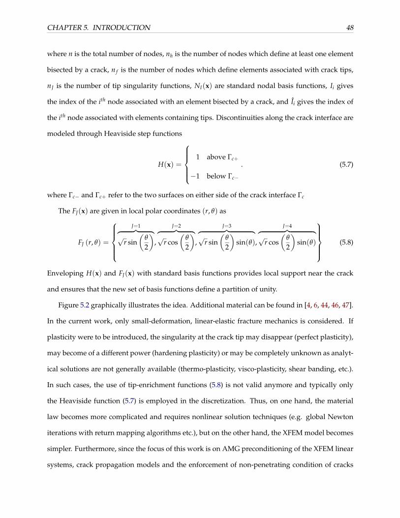
CHAPTER 5. INTRODUCTION 48
where n is the total number of nodes, nh is the number of nodes which define at least one element
bisected by a crack, n f is the number of nodes which define elements associated with crack tips,
nJ is the number of tip singularity functions, NI(x) are standard nodal basis functions, Ii gives
the index of the ith node associated with an element bisected by a crack, and Ii gives the index of
the ith node associated with elements containing tips. Discontinuities along the crack interface are
modeled through Heaviside step functions
H(x) =
1 above Γc+
−1 below Γc−
. (5.7)
where Γc− and Γc+ refer to the two surfaces on either side of the crack interface Γc
The FJ(x) are given in local polar coordinates (r, θ) as
FJ (r, θ) =
J=1︷ ︸︸ ︷
√r sin
(θ
2
),
J=2︷ ︸︸ ︷√
r cos(
θ
2
),
J=3︷ ︸︸ ︷√
r sin(
θ
2
)sin(θ),
J=4︷ ︸︸ ︷√
r cos(
θ
2
)sin(θ)
(5.8)
Enveloping H(x) and FJ(x) with standard basis functions provides local support near the crack
and ensures that the new set of basis functions define a partition of unity.
Figure 5.2 graphically illustrates the idea. Additional material can be found in [4, 6, 44, 46, 47].
In the current work, only small-deformation, linear-elastic fracture mechanics is considered. If
plasticity were to be introduced, the singularity at the crack tip may disappear (perfect plasticity),
may become of a different power (hardening plasticity) or may be completely unknown as analyt-
ical solutions are not generally available (thermo-plasticity, visco-plasticity, shear banding, etc.).
In such cases, the use of tip-enrichment functions (5.8) is not valid anymore and typically only
the Heaviside function (5.7) is employed in the discretization. Thus, on one hand, the material
law becomes more complicated and requires nonlinear solution techniques (e.g. global Newton
iterations with return mapping algorithms etc.), but on the other hand, the XFEM model becomes
simpler. Furthermore, since the focus of this work is on AMG preconditioning of the XFEM linear
systems, crack propagation models and the enforcement of non-penetrating condition of cracks

CHAPTER 5. INTRODUCTION 49
are not considered in this work.
(a) (b)
Figure 5.2: (a) Thick lines (red) depict cracks. Circles (green) and squares (red) give nodes en-riched by H(x) and FJ(x), respectively. (b) Computed stress σyy.
5.2.3 Levelset Functions
Levelset functions are now described as they play a role in the proposed multigrid algorithm.
The XFEM enrichment functions are developed by utilizing a normal levelset function ψ(x) and
a tangential levelset function φ(x) for each crack. These functions represent a local coordinate
system oriented along the crack with the origin at the crack-tip as shown in Figure 5.3. The signs of
the two functions effectively define four subregions of the domain. Levelset functions are used to
identify whether a crack completely cuts across an element (signifying that Heaviside enrichment
functions should be added) or whether the tip is located within an element (signifying that tip
enrichments should be added). This is done by simply evaluating ψ(x) and φ(x) at nodes defining
each element. H(x) is then determined by the sign of ψ(x) and the polar-coordinates (r, θ) for
specifying tip-enrichment are
r(x) =√
ψ2(x) + φ2(x)
θ(x) = tan−1(
ψ(x)φ(x)
).

CHAPTER 5. INTRODUCTION 50
This concept is generalized for multiple cracks using levelset functions defined for each crack
interface and each tip.
crack
ψ > 0, φ > 0
ψ > 0, φ < 0
ψ < 0, φ > 0
ψ < 0, φ < 0
Figure 5.3: Levelset functions for a single crack effectively subdividing Ω into 4 regions.
In the three-dimensional implementation of XFEM, only planar cracks bounded by general
polygonal edges are considered. The crack planes are represented in terms of the equation of a
plane (5.9). This facilitates the easy evaluation of the levelset functions with respect to the crack,
e.g., the left-hand-side of (5.9) is itself the normal levelset Φn(x) or the perpendicular distance
from the point x to the crack plane. The tangent levelset at a point Φt(x) denotes the perpen-
dicular distance to the closest edge of the crack along the crack plane. This is evaluated by first
projecting the point to the crack plane and then finding the perpendicular distance to the crack
edges represented by their corresponding line equations. The use of levelsets simplifies the iden-
tification of nodes to be enriched, the evaluation of the enrichment functions, and it also facilitates
the modeling of propagating cracks. A graphical representation of the levelset functions in three
dimensions is shown in Fig. 5.4.
Ax + By + Cz + D = 0 (5.9)
From a multigrid perspective, it is important to notice that the evaluation of levelset func-
tions requires coordinates. This type of information is not normally available within an algebraic
multigrid solver, but will be used in the proposed quasi-algebraic approach. In particular, fine
level coordinates and the levelset functions must be supplied along with the fine level discretiza-

CHAPTER 5. INTRODUCTION 51
Time = 0.00E+00
(a)
-5.59E+00
-4.47E+00
-3.35E+00
-2.23E+00
-1.10E+00
2.15E-02
1.14E+00
2.27E+00
3.39E+00
4.51E+00
5.64E+00
-6.72E+00
6.76E+00
_________________ DISPLACEMENT 1
Time = 1.00E+00
(b)
-9.58E+00
-8.07E+00
-6.55E+00
-5.04E+00
-3.52E+00
-2.01E+00
-4.95E-01
1.02E+00
2.53E+00
4.05E+00
5.56E+00
-1.11E+01
7.08E+00
_________________ DISPLACEMENT 2
Time = 1.00E+00
(c)
Figure 5.4: Levelsets in three dimensions (a) Mesh with crack (b) Φn contours (c) Ψn contours
tion. Additionally, the multigrid solver must project the fine level coordinates using a restriction
operator to coarser levels.
5.2.4 XFEM Linear System
The discrete solution in (5.6) within an element e may be written in terms of an augmented shape-
function matrix Nenr and the nodal degrees of freedom ueenr (which includes ue
I , aeI and be
I J):
uh(xe) = Neenrue
enr (5.10)
A gradient operator is applied to the augmented shape-function matrix to obtain
Beenr = ∇Ne
enr (5.11)
The XFEM stiffness matrix for the element e is then written as
Ae =∫
Ωe
(Beenr)
T DBeenrdΩe. (5.12)
It should be noted that numerical quadrature must take into account the presence of discontinuous
fields in Benr.
The global stiffness matrix A is obtained by the assembly of the element stiffness matrices.
Grouping all the standard and the enriched degrees of freedom results in a linear system of the

CHAPTER 5. INTRODUCTION 52
following form: Arr Arx
Axr Axx
ur
ux
=
fr
fx
(5.13)
where ur are associated with regular nodal degrees-of-freedom and ux are associated with special
degrees-of-freedom. The submatrix Arr is a standard nodal finite element discretization without
any cracks. Axx contains couplings between special degrees-of-freedom. This includes contribu-
tions from Heaviside and tip functions. Cracks within two dimensional domains can essentially
be mapped to a single dimension. Figure 5.5 illustrates an XFEM mesh and the corresponding
sparsity pattern of Axx. The dense portions are associated with the tip enrichments.
(a) (b) (c)
Figure 5.5: (a) XFEM mesh for a single crack (b) Sparsity pattern of A (c) Sparsity pattern of Axx

CHAPTER 5. INTRODUCTION 53
5.3 Algebraic Multigrid
The primary solution method used in this section is the algebraic multigrid method. It is well
known that multigrid is effective for solving many discrete partial differential equations, see
e.g, [14, 26, 69]. The key is to capture errors by utilizing multiple resolutions. High energy (or
oscillatory) components are reduced through a simple smoothing procedure, while low energy
(or smooth) components are tackled using an auxiliary lower resolution version. The scheme is
then applied recursively on the next coarser level. In standard multigrid, this is accomplished by
generating a hierarchy of meshes, G [k], corresponding to differing resolutions where the super-
script [k] indicates the grid level. Grid transfers are defined to move data between meshes and
discretizations are constructed on all meshes by either re-utilizing the discretization procedure or
Galerkin projection:
A[k+1] = (P[k])T A[k]P[k] (5.14)
where P[k] interpolates from G [k+1] to G [k] and A[k] is the discretization on G [k]. A sample multilevel
iteration is given in Figure 5.7 to solve
A[0]u[0] = b[0]. (5.15)
To complete the specification, relaxation R[k] and the P[k] must be defined. The key to fast
convergence is their complementary nature; errors not reduced by R[k] must be well interpolated
by P[k].
Algebraic multigrid differs in that the G [k]’s are not supplied and instead a notion of mesh is
developed from matrix data. This mesh is coarsened via graph algorithms, the P[k] are deduced
from algebraic principles, and used in conjunction with (5.14) to recursively generate a hierarchy.
In Chapter 6, an energy minimizing philosophy is followed to generate the P[k] and in Chapter 7,
a smoothed aggregation framework is adopted. The details of these particular philosophies are
not critical for this work. Energy minimization is chosen in the former case because nonstandard
prolongator sparsity patterns are easily incorporated. A brief description is given where super-

CHAPTER 5. INTRODUCTION 54
Figure 5.6: Multigrid V-cycle
// Solve A[k]u[k] = b[k]
procedure multilevel(b[k], u[k], k)u[k] = R[k](A[k], b[k], u[k]);if ( k 6= `)
r[k] = b[k] − A[k]u[k] ;u[k+1] = 0;u[k+1] =multilevel((P[k])Tr[k], u[k+1], k+1);u[k] = u[k] + P[k]u[k+1];u[k] = R[k](A[k], b[k], u[k]);
Figure 5.7: Multigrid V cycle consisting of ` levels to solve A[0]u[0] = b[0], where level 0 is the finestlevel.

CHAPTER 5. INTRODUCTION 55
scripts indicating level are omitted to simplify the presentation; more information can be found
in [78, 13, 41, 51, 12, 11, 75, 81, 34, 73]. The basic principle is that interpolation is chosen to mini-
mize the energy norm of prolongator basis functions subject to constraints. That is,
P = argminP
∑j‖Pj‖A and PBC = B, with P ∈ N , (5.16)
where Pj is the jth column of P, B (BC) is a column matrix of fine (coarse) level near null-space
modes, P ∈ N specifies that P’s sparsity pattern conforms to a specified form, N , and ‖v‖A ≡√
vT Av defines energy. B and BC have m columns so the relation PBC = B defines a set of m
vectors which P must exactly interpolate. In this work, these vectors are rigid body modes (i.e.,
m = 3 in two dimensions amd m = 6 in three dimensions).
The main idea is that interpolation complements relaxation. The more poorly an error mode
is reduced by fine level relaxation, the better it should be captured by interpolation so that it
can be reduced on a coarse level. Standard relaxation is ineffective for modes corresponding to
eigenvectors with small eigenvalues. This is most easily seen for Jacobi relaxation. For unattached
domains (no Dirichlet boundary conditions) the rigid body modes correspond to eigenvectors
with zero eigenvalue. Thus, the constraint PBC = B guarantees that these lowest energy modes
are exactly interpolated. It is also important that other modes corresponding to small eigenvalues
be well interpolated with interpolation accuracy of an eigenvector proportional to the reciprocal of
its associated eigenvalue [10, 43]. Energy minimization in conjunction with the constraint PBC = B
accomplishes this. Figure 5.8 provides an illustration. The figure shows two interpolants to a sine
wave, the eigenvector with the smallest nonzero eigenvalue of a one dimensional periodic Poisson
operator. While a constant is contained within the span of both sets of basis functions, the lower
energy basis functions more accurately capture the sine wave.
Sparsity patterns play a key role in this work. Recall that Pj is the jth coarse level basis function.
Thus,N determines the nonzero support associated with coarse level basis functions. The number
of nonzeros in the coarse level discretization matrix (defined via (5.14)) grows as overlap between
basis functions increases. However, less overlap gives rise to higher energy basis functions due to
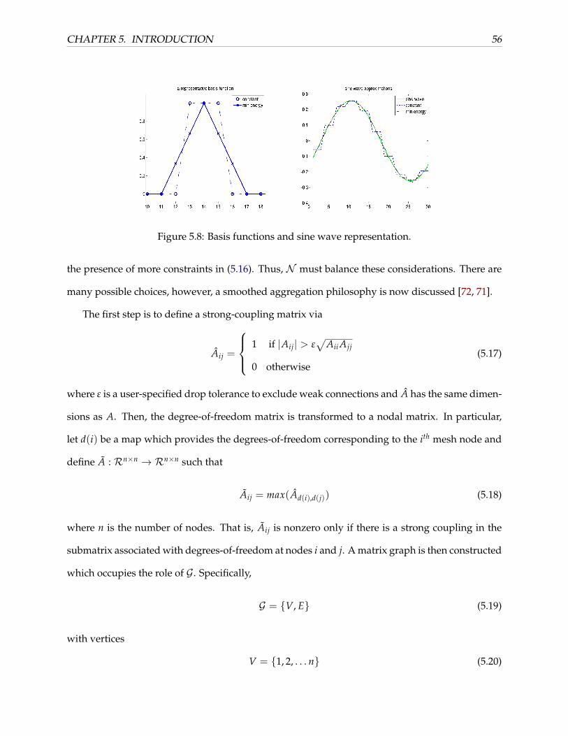
CHAPTER 5. INTRODUCTION 56
Figure 5.8: Basis functions and sine wave representation.
the presence of more constraints in (5.16). Thus, N must balance these considerations. There are
many possible choices, however, a smoothed aggregation philosophy is now discussed [72, 71].
The first step is to define a strong-coupling matrix via
Aij =
1 if |Aij| > ε
√Aii Ajj
0 otherwise(5.17)
where ε is a user-specified drop tolerance to exclude weak connections and A has the same dimen-
sions as A. Then, the degree-of-freedom matrix is transformed to a nodal matrix. In particular,
let d(i) be a map which provides the degrees-of-freedom corresponding to the ith mesh node and
define A : Rn×n → Rn×n such that
Aij = max(Ad(i),d(j)) (5.18)
where n is the number of nodes. That is, Aij is nonzero only if there is a strong coupling in the
submatrix associated with degrees-of-freedom at nodes i and j. A matrix graph is then constructed
which occupies the role of G. Specifically,
G = V, E (5.19)
with vertices
V = 1, 2, . . . n (5.20)
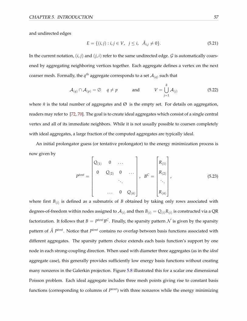
CHAPTER 5. INTRODUCTION 57
and undirected edges
E = (i, j) : i, j ∈ V, j ≤ i, Ai,j 6= 0. (5.21)
In the current notation, (i, j) and (j, i) refer to the same undirected edge. G is automatically coars-
ened by aggregating neighboring vertices together. Each aggregate defines a vertex on the next
coarser mesh. Formally, the qth aggregate corresponds to a set A(q) such that
A(q) ∩A(p) = ∅ q 6= p and V =n⋃
j=1
A(j) (5.22)
where n is the total number of aggregates and Ø is the empty set. For details on aggregation,
readers may refer to [72, 70]. The goal is to create ideal aggregates which consist of a single central
vertex and all of its immediate neighbors. While it is not usually possible to coarsen completely
with ideal aggregates, a large fraction of the computed aggregates are typically ideal.
An initial prolongator guess (or tentative prolongator) to the energy minimization process is
now given by
Ptent =
Q(1) 0 . . .
0 Q(2) 0 . . .
. . .
. . . 0 Q(n)
, BC =
R(1)
R(2)
. . .
R(n)
, (5.23)
where first B(i) is defined as a submatrix of B obtained by taking only rows associated with
degrees-of-freedom within nodes assigned to A(i) and then B(i) = Q(i)R(i) is constructed via a QR
factorization. It follows that B = PtentBC. Finally, the sparsity pattern N is given by the sparsity
pattern of A Ptent. Notice that Ptent contains no overlap between basis functions associated with
different aggregates. The sparsity pattern choice extends each basis function’s support by one
node in each strong-coupling direction. When used with diameter three aggregates (as in the ideal
aggregate case), this generally provides sufficiently low energy basis functions without creating
many nonzeros in the Galerkin projection. Figure 5.8 illustrated this for a scalar one dimensional
Poisson problem. Each ideal aggregate includes three mesh points giving rise to constant basis
functions (corresponding to columns of Ptent) with three nonzeros while the energy minimizing

CHAPTER 5. INTRODUCTION 58
basis functions have five nonzeros.
In practice, exact minimization is not needed and with initial guess given by (5.23) only a
couple of Krylov-like iterations are sufficient to approximate (5.16). Constraint satisfaction is also
straight-forward requiring solution of n linear systems of size m×m. The following reference [51]
is provided for additional aspects of energy minimization. fd
5.4 AMG for XFEM
In Fig. 5.9, the convergence of the solution obtained from a “black-box” application of AMG on
both an XFEM system and a regular FEM system is shown. The norm of the residual is plotted
against the number of conjugate gradient iterations with and without AMG preconditioning. It
may be observed from the figure that while the improvement in convergence is observed, AMG
is not as effective for XFEM as it is for FEM. To understand this, we must consider the sparsity
pattern algorithms described in the previous section in the context of XFEM. As mentioned pre-
viously, the grid transfer operators in AMG are obtained via the graph of the matrix constructed
from the couplings across various degrees of freedom in the linear system. For a stiffness matrix
generated via XFEM, strong couplings do exist across degrees of freedom corresponding to nodes
of an enriched element, even on opposite sides of a crack. This indicates that aggregates can span
across the cracks, leading to an inaccurate representation of the discontinuities on coarse levels.
Additionally, the variability of the number of degrees of freedom in XFEM enriched nodes, pose
problems for the AMG preconditioner. Further elaborations on the mismatch of XFEM linear sys-
tems for AMG are provided in Chapters 6 and 7 in addition to proposed methods to alleviate the
difficulties.

CHAPTER 5. INTRODUCTION 59
0 50 100 150 200 25010
−8
10−7
10−6
10−5
10−4
10−3
10−2
10−1
100
101
Number of Iterations
Res
idua
l Nor
m
FEM CG (unpreconditioned)FEM With AMG preconditioningXFEM With AMG preconditioningXFEM CG (unpreconditioned)
Figure 5.9: Convergence of CG with and without preconditioning

CHAPTER 6. XAMG-I 60
Chapter 6
AMG for XFEM - I
In this chapter, a new quasi-algebraic multigrid method that is suitable for linear systems obtained from discretizing
fracture mechanics problems using the extended finite element method is presented. This new method derives from
the application of AMG on the Schur Complement of the XFEM matrix. Primarily two-dimensional, static and
linear-elastic fracture mechanics implemented on the MATLAB platform is considered. The inputs from co-authors of
the paper (Hiriyur et. al. [30]) from which this chapter is reproduced are gratefully acknowledged.
6.1 Schur complement of XFEM matrix
We now consider application of the algebraic multigrid idea to the 2× 2 block system which is
repeated here for reference: Arr Arx
Axr Axx
ur
ux
=
fr
fx
. (6.1)
Unfortunately, the special degrees-of-freedom pose potential problems for algebraic multigrid.
One difficulty is the treatment of low energy modes. Recall that constants and more generally
rigid body modes correspond to low energy modes. Standard relaxation is not effective on these
components and so they must be accurately represented on a coarse level. In the XFEM context,
it is natural to ask whether cracks introduce additional low energy modes which must be treated
with care. Suppose, for example, that a crack completely traverses an unattached structure (i.e.
without Dirichlet boundary conditions) thereby dividing it into two floating subdomains. This

CHAPTER 6. XAMG-I 61
division doubles the number of rigid body modes reflecting the independent movement of the
individual subdomains. This larger space can be represented by defining a set of vectors corre-
sponding to standard rigid body modes and augmenting these with the same set of vectors except
that entries associated with one of the floating subdomains are redefined to be zero. All of these
low energy vectors must be well-represented in the range of interpolation, but unfortunately the
new vectors are discontinuous at the crack interface. It is unlikely that a standard AMG prolon-
gator will preserve this discontinuity when interpolating between coarse and fine meshes. Thus,
these discontinuous modes are not well-addressed by either standard relaxation or the coarse level
correction. Of course, cracks do not always completely traverse the domain. While prolongation
for partial crossings is somewhat less clear, it seems natural that interpolation should preserve
local discontinuities of rigid body modes across crack boundaries. This implies that coarse values
on one side of a crack should not be used to interpolate to fine values on the other side of a crack
when these values are far from a crack tip.
Another AMG difficulty arises from having a variable number of degrees-of-freedom (dofs)
at each fine level node. This variability defeats capabilities within most multigrid codes for ad-
dressing PDE systems. In particular, PDE systems are often tackled by grouping dofs at each
node (as described for creating the nodal matrix A in Section 5.3). Most AMG codes, however,
assume that the number of dofs per node is constant and so in this case blocking cannot be uti-
lized. Blocking information can be ignored, but this is akin to treating a PDE system as a scalar
PDE. Specifically, blocking is often used to guarantee exact interpolation of constant functions for
each degree-of-freedom at coarse nodes and so this is lost if blocking is not done. In the specific
case of energy minimization, interpolation of constants is accomplished by the rigid body mode
constraints. However, it is not clear how B should be defined for degrees-of-freedom associated
with enrichment functions.
One possible remedy is to algebraically eliminate special degrees-of-freedom from the system.

CHAPTER 6. XAMG-I 62
That is to instead consider the Schur complement
Sur = fr − Arx A−1xx fx with S = Arr − Arx A−1
xx Axr. (6.2)
Figure 6.1 illustrates a single crack and the stencil at an unknown near the left side of the crack.
Figure 6.1: Graphic illustration of Schur complement stencil just left of a crack.
Specifically, a matrix row is displayed of the Schur complement which has undergone symmetric
diagonal scaling. The figure plots absolute value of entries associated with the first degrees-of-
freedom at corresponding nodal locations. The largest entry corresponds to the matrix diagonal.
Entries to the left correspond to couplings away from the crack while those to the right are cou-
plings across the crack. The figure illustrates that this row contains nonzeros along the crack in-
terface but that these nonzeros are small far from the diagonal entry and almost negligible across
the crack. This reflects the nature of the problem in that adjacent dofs on opposite sides of a crack
are actually quite distant in terms of the underlying physics.
Removal of special degrees-of-freedom effectively renders the problem amenable to algebraic
multigrid methods. Table 6.1 illustrates convergence data for fairly standard 2-level AMG al-
gorithms applied directly to the full system as well as applied to the Schur complement. Two

CHAPTER 6. XAMG-I 63
different AMG versions are shown for the full system. The variable block AMG maintains the
relationship between dofs and nodes while scalar AMG does not. The Schur complement AMG
uses constant block sizes of two. In each case one Krylov-like iteration [51] is used to improve the
initial prolongator and generate a final prolongator that approximates (5.16). For scalar AMG and
variable block AMG, B(BC) are taken to be zero for enriched degrees-of-freedom. All AMG meth-
ods drop weak connections during prolongator construction using ε = 10−2. This dropping does
not have a big effect on scalar or variable block AMG, but this dropping effectively removes cou-
pling across cracks within the Schur AMG method. In addition to dropping small entries, Schur
complement nonzeros that are not present in Arr are removed when constructing S. Ensuring
that S does not have large stencils avoids large aggregates and sparsity patterns with too much
overlap.
In all experiments, a direct solver is always used for coarse level relaxation while on finer levels
one symmetric block Gauss-Seidel defines the R[k] where blocks are associated with grouping
dofs at nodes for the Schur AMG and block AMG. The block size is one for scalar AMG. “-”
indicates that preconditioned conjugate gradient did not achieve a residual reduction of 10−8 in
200 iterations. AMG V cycles are used for all the results presented here. It is clear from Table 6.1
that AMG applied directly to the full system is problematic while AMG applied to the Schur
complement is ideal. The key reason for this is that the Schur complement method does not
coarsen enrichment unknowns and that Schur complement prolongators do not interpolate across
cracks. This means that the interpolation respects the XFEM discontinuities.
Table 6.1: PCG iterations for different AMG approaches on a six crack problem (case 5b in Fig-ure 6.3i).
Mesh Scalar AMG Variable Block AMG AMG on Schur Complement30×30 180 89 1060×60 - 103 1190×90 - 114 11120×120 - 126 12
The remainder of this work focuses on an algebraic multigrid method which avoids the ex-

CHAPTER 6. XAMG-I 64
plicit computation of the Schur complement. This is particularly important for large parallel three
dimensional calculations with many cracks. It should be noted that Schur complement multilevel
methods have been considered in domain decomposition where unknowns within subdomain in-
teriors are removed from the linear system. In this case, spectral equivalence with the original
operator is often used to avoid an explicit Schur complement, though the Schur complement can
be efficiently computed for the Galerkin projection within a domain decomposition scheme [15].
6.2 A new AMG method
While avoiding the explicit computation of S, an algorithm with similar convergence character-
istics to that of applying AMG to the Schur complement is sought . To this end, three Lemmas
relating AMG applied to the Schur complement and AMG applied to the 2× 2 block linear system
are presented. Equivalences between Schur complements and full systems have been explored in
a non-multilevel context in [33].
Lemma 6.2.1. Schur complement/projection commutativity. Consider (6.1) and its associated Schur com-plement given by (6.2). Let P be a prolongation operator used in a Schur complement multigrid algorithmand let
P =
[P 00 I
](6.3)
be a prolongation operator used to project the full system. Then, the projected Schur complement,
SH = PTSP ,
and the Schur complement of the projected full system are equivalent.
Proof. Follows by comparison of the two coarse level Schur complements which in both cases isgiven by PT ArrP −PT Arx A−1
xx AxrP .
Remark 6.2.2. The above two-level result generalizes to a multilevel setting using recursive arguments.
It is important to notice the computational differences between projecting the Schur comple-
ment versus taking the Schur complement of a projected system. In both cases, the following
quantity is computed
PT Arx A−1xx AxrP .

CHAPTER 6. XAMG-I 65
The difference is in the order in which operations occur. Projection of the full system effectively
performs the product AxrP . The result has significantly fewer columns and so application of A−1xx
is less expensive than first forming A−1xx Axr.
Lemma 6.2.3. Assume the full linear system (6.1) is given along with S = Arr − Arx A−1xx Axr and a
reduced right hand side fr = fr − Arx A−1xx fx. Consider two relaxation procedures corresponding to the
reduced system and the full system:
Reduced Relaxationur ← ur + M−1
rr rr
Full System Relaxation
(a) ux ← A−1xx ( fx − Axrur)
(b)[
urux
]←
[urux
]+
[Mrr 0Axr Axx
]−1 [ rrrx
]where rr denotes the residual associated with the Schur system while rr and rx give residual components forthe full system. Mrr is non-singular and typically approximates Arr. Further, assume that both proceduresbegin with identical initial guesses for the regular degrees-of-freedom (i.e., ur = ur on entry). Then, thefinal ur and ur produced by Reduced Relaxation and by Full System Relaxation are equivalent and rx = 0after completion of both step (a) and (b) of Full System Relaxation.
Proof. Verification of rx = 0 after step (a) follows trivially from the definition of rx and the as-signed value to ux. Verification after step (b) is seen by transforming to a residual update. This isdone by pre-multiplication of step (b) with the 2× 2 block system and subtracting this from theright hand side. This results in[
rrrx
]←[
rrrx
]−[
Arr ArxAxr Axx
] [Mrr 0Axr Axx
]−1 [ rrrx
]where it may be noted that the second matrix is block triangular so the diagonal blocks can simplybe inverted. It follows that rx = 0. Finally, substitution of ux = A−1
xx ( fx − Axrur) into rr =fr − Arrur − Arxux reveals that if ur = ur on entry, then rr = rr after step (a) of Full SystemRelaxation. From this it follows that ur = ur at termination.
Notice that repeated Full System Relaxation sweeps require that step (a) only be performed on
the first sweep as it is only before the first step of the first sweep that rr might be nonzero. Further
notice that the initial value of ux is not used within Full System Relaxation.
Lemma 6.2.4. Assume the full linear system (6.1) is given along with a reduced right hand side fr = fr −Arx A−1
xx fx and S = Arr − Arx A−1xx Axr. Consider two m-level multigrid V cycle procedures as described
in Figure 5.7 which are fully defined by relaxation and grid transfers; one applied to the Schur complementand the other applied to the full system.
Reduced Multigrid

CHAPTER 6. XAMG-I 66
• P [k] prolongates from level k+1 to level k
• relaxation consists of ν > 0 pre- and post-sweeps given by
u[k]r ← u[k]
r + (M[k]rr )−1r[k]r
Full System Multigrid
• prolongation from level k+1 to level k is accomplished via[P [k] 0
0 I
].
• relaxation consists of ν > 0 pre- and post-sweeps given by
(a) u[k]x ← (A[k]
xx)−1( f [k]x − A[k]
xr u[k]r )
(b)
[u[k]
r
u[k]x
]←
[u[k]
r
u[k]x
]+
[M[k]
rr 0A[k]
xr A[k]xx
]−1 [r[k]r
r[k]x
]
where the superscript [k] again denotes grid level. Then, under the additional assumption that both proce-dures begin with the same initial guess for regular degrees-of-freedom (i.e. u[1]
r = u[1]r on entry), the two
multigrid procedures produce identical solutions for the regular degrees-of-freedom at termination.
Proof. The Lemma obviously holds for m = 1 as Lemma 6.2.3 directly applies when relaxation isused on the coarsest level and a direct solver is simply a special case of Lemma 6.2.3 associatedwith M[m]
rr = S[m]. The proof is completed by induction. Assume the Lemma is true for m− 1 levelversions of the multigrid procedures, and show that the Lemma holds for m level versions of themultigrid procedures.
For the finest grid (i.e. k = 1) pre-relaxation of the m level AMG versions, Lemma 6.2.3 appliesso that after pre-relaxation u[1]
r = u[1]r and r[1]x = 0. A recursive invocation of the multilevel proce-
dures follows the finest grid relaxation and this defines the second level of the m level methods.This recursive invocation, however, also coincides with the finest grid of a m− 1 level multigridmethod. Thus, the solutions coincide after this recursive invocation if we use the assumption thatthe Lemma is true for m − 1 versions of the multigrid procedures. To apply the m − 1 versionof the Lemma, however, the Lemma’s assumptions (initial guesses, right hand sides, and linearsystems) hold for this recursive invocation must first be validated. That is,
u[2]r = u[2]
r for the initial guessesS[2] = A[2]
rr − A[2]rx (A[2]
xx)−1A[2]
xr
f [2]r = f [2]r − A[2]rx (A[2]
xx)−1 f [2]x
(6.4)
The first statement is trivially true as coarse level initial guesses (u[2]r and u[2]
r ) are taken as zerowithin a V cycle procedure. The second statement follows directly from Lemma 6.2.1. After pre-relaxation, the projected residual of the reduced system is the right hand side for the next level

CHAPTER 6. XAMG-I 67
and sof [2]r = (P [1])T( f [1]r − S[1]u[1]
r ),= (P [1])T( f [1]r − A[1]
rx (A[1]xx)−1 f [1]x − S[1]u[1]
r ),= (P [1])T( f [1]r − A[1]
rx (A[1]xx)−1 f [1]x − A[1]
rr u[1]r + A[1]
rx (A[1]xx)−1A[1]
xr u[1]r ).
The first component of the projected residual for the full system is
f [2]r = (P [1])T( f [1]r − A[1]rr u[1]
r − A[1]rx u[1]
x ),= (P [1])T( f [1]r − A[1]
rr u[1]r − A[1]
rx (A[1]xx)−1( f [1]x − A[1]
xr u[1]r )),
= f [2]r
where r[1]x = 0 after pre-relaxation is used to eliminate u[1]x above. As f [2]x = Ir[1]x = 0, it follows
that (6.4) holds and so the interpolated corrections coincide (P [1]u[2]r = P [1]u[2]
r ) after recursiveinvocation as the m − 1 level version of the Lemma is assumed. The proof is completed by rec-ognizing that the assumptions of Lemma 6.2.3 are satisfied for post-relaxation and so that V cycleterminates with identical solutions for the regular degrees-of-freedom.
The last Lemma establishes that a multigrid cycle can be constructed for the 2× 2 block system
which is completely equivalent to multigrid applied directly to the explicit Schur complement.
To do this without forming an explicit Schur complement, however, requires that M[k]rr and P [k]
be defined without relying on S[k]. Additionally, an efficient procedure for solving systems of
the form A[k]xxw = b is needed within relaxation. Unfortunately, M[k]
rr and P [k] would normally
employ a Schur complement matrix in their definition and so it is not practical to make an entirely
equivalent multigrid cycle based on the 2× 2 block system. Instead, an approximation is pursued.
Prolongator construction is based on energy minimization which in turn utilizes S in the defi-
nition of energy and in the algorithm for building a prolongator sparsity pattern via SPtent where
again superscripts indicating level have been dropped. Recall that in the experiments associated
with Table 6.1, S is defined by not only removing small entries from S, but also by removing en-
tries that do not appear in Arr. This second removal avoids large stencils which give rise to large
aggregates and dense sparsity patterns. First, consider how S and Arr differ. In particular, the
sparsity pattern of S is identical to Arr for entries associated with mesh locations far from any
crack. This is due to the fact that Arx and Axr contain only nonzeros for dofs adjacent to cracks.
For each crack, S contains a dense block for all dofs along the crack. However, all entries not ap-

CHAPTER 6. XAMG-I 68
pearing in Arr were removed when generating Table 6.1. This means that the difference between S
and Arr is the coupling across cracks. As Figure 6.1 illustrated, this coupling is small in the Schur
complement matrix and so it is eliminated when small entries are dropped. To mimic this effect
without forming a Schur complement, the definition of Arr is modified so that crack couplings are
removed. This modification affects the aggregation (which gives rise to Ptent) and the resulting
sparsity pattern given by ArrPtent (see Figure 6.2).
The only remaining occurrence of the explicit Schur complement during prolongator construc-
tion is the use of S in the definition of energy. This is also replaced with Arr. As stated earlier, Arr
and S are identical far from cracks. They are most dissimilar for nonzeros corresponding to crack
crossings. However, these nonzeros do not play a significant role in the energy minimization pro-
cess as crack crossings are not permitted in prolongator basis functions (due to truncation of the
prolongator sparsity pattern). Numerical justification is given shortly to access the effects of these
approximations.
To complete the multigrid cycle, relaxation must be defined without forming Schur comple-
ments. Assume, for now, that a factorization of Axx is available and so the only remaining issue is
generating the Mrr. If a Jacobi smoother is used, then Mrr is the diagonal of the Schur complement.
Once again, far from cracks Arr and S correspond. It is only for degrees-of-freedom adjacent to
crack that they differ. In principle, one could use a technique such as probing [59] to approximate
this diagonal. Probing basically combines coloring techniques with matrix-vector products to ap-
proximate a matrix. As will be shown, however, simply using the diagonal of Arr to define Mrr
(e.g., taking the diagonal for Jacobi smoothing or the lower triangular part for Gauss-Seidel) does
not seriously impact convergence.
6.3 Algorithm Details
The new AMG algorithm uses a hybrid prolongator given by (6.3). P is defined by applying a
standard algebraic multigrid algorithm to a modified form of Arr which is intended to mimic the
Schur complement by dropping entries associated with crack crossings. This is done with the

CHAPTER 6. XAMG-I 69
Figure 6.2: Sparsity Pattern Modification: Blue circles indicate sparsity pattern of a single prolon-gator column and black squares are removed pattern entries due to a crack.
help of the function Drop. A simplistic version is detailed in Algorithm 6.3.1. As φ and ψ require
coordinates, these are projected using a restriction operator based on averaging coordinate values
at all nodes within an aggregate to define the associated coordinate location on the coarse level.
Algorithm 6.3.2 summarizes prolongation construction.
Algorithm 6.3.1 Arr ← Drop(Arr, BlkSize, coords, tol, φ, ψ)
Require: matrix Arr with constant blocksize of BlkSize.Require: coordinate locations coords of nodesRequire: drop tolerance tol for removing small entriesRequire: levelset functions φ, ψ representing cracks
Arr ← StandardDrop(Arr, tol)for i = 1 to dimension(Arr) do
Ci ← j | [Arr]ij 6= 0(x1, y1)← (coords(i/BlkSize, 1), coords(i/BlkSize, 2))for j ∈ Ci do(x2, y2)← (coords(j/BlkSize, 1), coords(j/BlkSize, 2))for each crack c do
if ψc(x1, y1)ψc(x2, y2) < 0 AND φc(x1, y1) ≤ 0 then
[Arr]ij ← 0[Arr]ji ← 0
end ifend for
end forend for
Algorithm 6.3.3 depicts the relaxation which avoids explicit construction of the Schur comple-

CHAPTER 6. XAMG-I 70
ment and uses Arr to define Mrr. Table 6.2 assesses the individual affects of these different approx-
imations on the convergence rate of the overall method. In particular, CG with AMG precondi-
tioning is applied to a problem with six cracks (case 5a depicted in Figure 6.3i). P(C, G) indicates
that the prolongator was generated via energy minimization using the matrix C in its definition of
energy and using G to generate the sparsity pattern. In the table, Arr refers to the modified form
with crack crossings removed. The second and third columns give preconditioned AMG iterations
applied to the true Schur complement with relaxation as defined in Lemma 6.2.3. The remain-
ing columns refer to the hybrid prolongator with different forms of Hybrid Smoother relaxation.
Specifically, the fourth column is associated with the Hybrid Smoother in Lemma 6.2.3 while the
rightmost columns use either symmetric Gauss-Seidel (indicated by GS) or a direct solver to de-
fine relaxation components. AMG V cycles are used for all the results presented here. The reader
should note that the third and fourth columns are identical. When Arr is used instead of S to
generate sparsity patterns for the Schur method, this does in fact give identical convergence to the
hybrid method in column four and these two variants correspond to Lemma 6.2.4. Overall, it is
clear that there is a very modest increase in the number of iterations reading from left to right cor-
responding to different approximations, and that the rightmost column still appears to be nearly
mesh independent.
Table 6.2: Assessment of Schur complement approximations for case 5a in Figure 6.3i
Schur Hybridmesh P(S, S) P(Arr, S) P(Arr, Arr) P(Arr, Arr) P(Arr, Arr)size Lem. 6.2.3 Lem. 6.2.3 Alg. 6.3.3 with Alg. 6.3.3 with Alg. 6.3.3 with
relaxation relaxation Rx as direct Rx as direct Rx as GSwith Mrr as with Mrr as solver andRr solver andRr on Axx andRr
GS on S GS on S as GS on S as GS on Arr as GS on Arr
302 10 11 14 14 18602 11 11 13 13 17902 11 11 13 13 171202 12 12 13 13 17

CHAPTER 6. XAMG-I 71
Algorithm 6.3.2 P← ConstructP(B, Arr, BlkSize, coords, tol, φ, ψ, s)Require: column matrix B of rigid body modesRequire: matrix Arr with constant blocksize of BlkSizeRequire: coordinate locations coords of nodesRequire: drop tolerance tol for removing small entriesRequire: levelset functions φ, ψ representing cracksRequire: number of enrichment degrees-of-freedom s
Arr ← Drop(Arr, BlkSize, coords, tol, φ, ψ) via Algorithm 6.3.1Arr ← MakeNodalMatrix(Arr, BlkSize)A(1) . . .A(n)← StandardAggregation(Arr)
Ptent, BC ← StandardInitialProlongator(B,A(1) . . .A(n), BlkSize)N ← Pattern(Arr Ptent)P ← StandardEnergyMinimization(Arr, Ptent, B, BC,N )
P ←[P 0
0 Is
]where Is is an s× s identity matrix
coords ← AverageCoords(coords,A(1) . . .A(n))
Algorithm 6.3.3 u←HybridSmoother(A, u, f ,Rr,Rx, s)Require: matrix A with s degrees-of-freedom corresponding to enrichmentsRequire: initial guess uRequire: right hand side fRequire: SubSmoothers: Rr,Rx
Apply one sweep ofRx to smooth on: Axxux = fx − AxrurApply one sweep ofRr to smooth on: Arrur = fr − ArxuxApply one sweep ofRx to smooth on: Axxux = fx − Axrur

CHAPTER 6. XAMG-I 72
6.4 Numerical Results
Crack configurations are shown in Figure 6.3 corresponding to different numbers of cracks, cracks
of different length, different crack orientations, and completely interior cracks. The aggregation of
a few sample cases is displayed in Figure 6.4. Aggregates for horizontal cracks tend to have some-
what regular rectangular shapes (though some aggregates are larger than others). Aggregates for
inclined cracks tend not to follow any particular pattern (though no aggregates cross cracks due
to the levelset dropping).
The total number of preconditioned conjugate gradient iterations are presented in Table 6.3 in
order to achieve a residual reduction of 10−8. In all cases, the initial guess is zero and the right
hand side corresponds to fixed Dirichlet boundary condition on the bottom boundary followed
by Neumann conditions on all other boundaries. The side edges are traction free while uniform
normal traction is applied on the top edge. VBlk AMG corresponds to relatively standard alge-
braic multigrid where all dofs at a common geometric position are blocked together. These blocks
are used when coarsening (or aggregating) as well as during the block symmetric Gauss-Seidel
relaxation. The Quasi AMG method is the new method advocated in this work. It uses the hybrid
prolongator described in Algorithm 6.3.2 in conjunction with the specialized dropping procedure
given in Algorithm 6.3.1. A constant block size of two (at the finest level) is used to construct P .
The previously discussed hybrid relaxation scheme is not employed in any of these experiments.
This was primarily a theoretical tool that helped establish the equivalence with the Schur com-
plement AMG method. Instead, point symmetric Gauss-Seidel relaxation is employed within the
new Quasi AMG method and within the HybridStandard AMG method to be discussed. Only the
VBlk AMG uses the more expensive block symmetric Gauss-Seidel relaxation. The HybridStan-
dard AMG method also uses Algorithm 6.3.2 to build a hybrid prolongator. The key difference,
however, is that specialized dropping which removes crack crossing is not used when construct-
ing Arr. Instead, standard dropping given by (5.17) is used for HybridStandard AMG as well as
for VBlk AMG. This makes both VBlk AMG and HybridStandard AMG truly algebraic as levelset

CHAPTER 6. XAMG-I 73
(a) Case 1a (b) Case 1b (c) Case 1c
(d) Case 2a (e) Case 2b
(f) Case 3a (g) Case 3b (h) Case 4
(i) Case 5a (j) Case 5b
Figure 6.3: Test crack configurations (1a,b,c) Single propagating crack (2a,b) Two edge cracks (3a,b)Six edge cracks (4) Six interior cracks (5a,b) Inclined cracks

CHAPTER 6. XAMG-I 74
Figure 6.4: Sample aggregates. Each grid point is colored corresponding to the aggregate thatcontains it. The red lines represent cracks.
functions and coordinates are not needed. For standard dropping in all methods, ε is 8 · 10−2.
Similar to Quasi AMG, a block size of two is used during coarsening. AMG V cycles are used for
all the results presented here. In all cases, one Krylov-like iteration is used to improve the ini-
tial prolongator and generate a final prolongator that approximates (5.16). For VBlk AMG, B(BC)
are taken to be zero for enriched degrees-of-freedom. A direct solver is always used for coarsest
level relaxation. “-” indicates that preconditioned conjugate gradient did not converge in 200 iter-
ations. It is clear from the results that only the Quasi AMG method gives acceptable performance
and that the number of iterations required for convergence does not grow. It is emphasized that
the performance of standard AMG deteriorates as the number of cracks increase while the Quasi
AMG method is not affected as much. Therefore the computational efficiencies introduced by the
proposed method are further advantageous when multiple cracks are present.
Table 6.4 concludes with AMG operator complexities for the Quasi AMG method associated
with Case 5b. Operator complexity is normally defined as
complexity =∑`
k=1 nnz(A[k])
nnz(A[1])(6.5)
where ` is the total number of multigrid levels and nnz(C) is the number of nonzero entries in
the matrix C. Thus, the operator complexity gives a measure of how much additional memory
is required to store the coarse level discretization operators as well as the computational work

CHAPTER 6. XAMG-I 75
Tabl
e6.
3:Pr
econ
diti
oned
CG
iter
atio
nsfo
rtw
o-di
men
sion
alpr
oble
ms
Mes
hC
ase
#of
dofs
VBl
kA
MG
Hyb
rid
Stan
dard
AM
G
Qua
siA
MG
Cas
e#
ofdo
fsV
Blk
AM
GH
ybri
dSt
anda
rdA
MG
Qua
siA
MG
302
1a
1900
2813
11
3a
2676
154
-16
602
7372
2915
1087
8412
7-
1490
216
444
4118
1418
492
--
3212
0229
116
4120
1431
800
--
2830
2
1b
1948
2422
11
3b
2772
--
1860
274
6824
2912
8808
--
2190
216
588
4037
1818
444
--
3412
0229
308
3842
1731
680
--
2630
2
1c
1996
3131
13
4
2436
116
107
1560
275
6432
4314
8328
102
154
2190
216
732
5455
2117
820
167
199
2812
0229
500
5262
2030
912
173
-25
302
2a
2132
6457
15
5a
2436
8076
1260
278
0852
8014
8328
9110
713
902
1708
410
010
226
1782
013
513
419
1202
2996
010
611
723
3091
215
315
519
302
2b
2676
7359
16
5b
2436
8981
1660
287
8472
8117
8328
103
116
1590
218
492
109
108
2717
820
149
147
2012
0231
800
108
123
2430
912
165
170
19

CHAPTER 6. XAMG-I 76
associated with operating on a hierarchy as opposed to a single level method. In particular, the
work per V cycle is proportional to the operator complexity. In Table 6.4 the column labeled “full
complexity” corresponds to this. The “sub-block complexity” column redefines nnz(A[k]) so that
nonzeros in A[k]xx are excluded. As the Axx block is identical on all levels, it need not be replicated
each time within the multigrid hierarchy. Thus, sub-block complexity more accurate reflects the
required storage for a more sophisticated implementation. In general, complexities less than two
are considered acceptable which is the case for the presented results. Obviously, this depends on
the number of cracks present in the problem. It should be noted that these operator complexities
are about 25% higher than standard smoothed aggregation operator complexities for model two
dimensional elasticity problems. Thus, we would expect that one iteration of the Quasi AMG
method would roughly be about 25% more costly than a standard smoothed aggregation iteration.
Table 6.4: AMG operator complexities for Quasi AMG on Case 5b.
Mesh # of levels full complexity sub-block complexity30× 30 2 1.673 1.60760× 60 3 1.815 1.71690× 90 3 1.650 1.583
120× 120 4 1.699 1.621
6.4.1 Application in 3D
The methods developed in this work are primarily motivated by three dimensional simulations
where iterative methods are essential due to the high costs associated with direct solvers. How-
ever the main concern in 3D is that cracks become essentially two-dimensional i.e. surface entities,
and tips become one-dimensional. To validate the applicability of the proposed AMG solution
process for three dimensional problems, a sample block with three planar cracks is considered as
shown in Figure 6.5. In this case, only Heaviside enrichments are considered. Table 6.5 shows the
number of preconditioned CG iterations for various mesh-sizes and the number of AMG levels
employed. The AMG operator complexities - full (FC) and sub-block (SC), are presented in Ta-

CHAPTER 6. XAMG-I 77
ble 6.6. From the table, it may be observed that iteration counts remain nicely behaved, though
Time = 0.00E Time = 0.00E
(a)
8.33E+04
1.67E+05
2.50E+05
3.33E+05
4.17E+05
5.00E+05
5.83E+05
6.67E+05
7.50E+05
8.33E+05
9.17E+05
0.00E+00
1.00E+06
_________________ DISPLACEMENT 3
Time = 0.00E+00
-3.20E-01
1.55E+00
3.42E+00
5.29E+00
7.16E+00
9.03E+00
1.09E+01
1.28E+01
1.46E+01
1.65E+01
1.84E+01
-2.19E+00
2.02E+01
_________________ DISPLACEMENT 3
Time = 0.00E+00
(b)
Figure 6.5: (a) XFEM 3D mesh for a three crack problem (b) XFEM solution - displacement contours
Table 6.5: Preconditioned CG iterations for a three-dimensional problem
Mesh # of 2-level 3-level 4-level 5-leveldofs nits nits nits nits
103 4818 15 16203 33015 19 20 21403 218988 20 24 25 25603 722559 29
Table 6.6: AMG operator complexities for a three-dimensional problem
Mesh # of 2-level 3-level 4-level 5-leveldofs FC SC FC SC FC SC FC SC
103 4818 1.71 1.66 2.03 1.86203 33015 1.69 1.65 2.01 1.89 2.17 1.94403 218988 1.53 1.51 1.70 1.63 1.81 1.70 1.87 1.71603 722559 1.91 1.75
there is a slight growth as we refine. While the AMG operator complexities are quite reasonable,
they are higher than in the two dimensional case. The bulk of this is due to a technical issue in how

CHAPTER 6. XAMG-I 78
sparsity patterns are chosen and a somewhat inefficient aggregation algorithm. In particular, the
coarse operators have six degrees-of-freedom per node as opposed to three degrees-of-freedom
on the fine mesh due to the presence of six near null space vectors in three dimensions. This six
degrees-of-freedom per node is certainly not required and was only used to mimic smoothed ag-
gregation sparsity patterns. Based on prior non-fracture experimentation, it is suspected that a
more judicious pattern choice could noticeably lower complexities without significantly affecting
convergence, though further experimentation would be needed to verify this.
6.5 Extensions
The algorithm proposed in this work only applies coarsening to the Arr block of the XFEM linear
system. When the percentage of elements with enrichment functions is relatively modest, then
this type of algorithm is indeed practical (though there may be some parallelization concerns).
However, when the dimensions of Axx are relatively large, the lack of coarsening on the enrich-
ment degrees-of-freedom can become prohibitively expensive. This often happens when many
micro cracks are modeled or in three dimensions when cracks are surface entities. Preliminary
experience indicates that coarsening degrees-of-freedom associated with Heaviside enrichments
is not problematic. In particular, a block diagonal prolongator can be developed using P for reg-
ular dofs, P for Heaviside enrichment dofs, and Is for tip enrichment dofs where s is the number
of dofs with tip enrichments. Somewhat standard AMG methods can then be used to develop
P . This is due to the fact that the associated basis functions (which are the product of Heavi-
side functions and standard nodal basis functions) are quite similar to typical finite element basis
functions. Additionally, Heaviside dofs in Axx on one side of a crack do not contain direct cou-
plings to Heaviside dofs on the other side of a crack and so the crack crossing issues do not arise.
These couplings are illustrated in Figure 5.5 where the first narrow banded section corresponds to
the lower crack interface while the second narrow band corresponds to the upper crack interface.
Coarsening of tip functions appears to be much more problematic as they are fairly nonstandard
and highly ill-conditioned basis functions.
CHAPTER 7. XAMG-II 79
Chapter 7
AMG for XFEM - II
In this chapter, a new algebraic multigrid method that is suitable for linear systems obtained from discretizing
fracture mechanics problems using the extended finite element method is presented. This method is based on the
transformation of the XFEM linear system into an alternate representation based on the Phantom-node variant of
XFEM. Three-dimensional cracks, nonlinear material properties and MPI based parallel implementation on the
parFEAP and Trilinos platforms are considered. The inputs from authors of the paper (Gerstenberger et. al. [25])
which forms the basis for this chapter are gratefully acknowledged.
7.1 Introduction
Similar to Chapter 6, here an alternative approach will be discussed to adapting algebraic multi-
grid (AMG) such that it is suitable for linear systems arising from fracture mechanics problems
modeled using the extended finite element method (XFEM). In this chapter, an extension of the
method proposed in Gerstenberger and Tuminaro [25] to fracture problems in three dimensions is
presented. In addition, nonlinear materials and parallel implementation so that the method can
be scaled to studying fracture problems at a larger scale are considered.
Here’s a brief outline of this chapter: In Section 7.2.1 a phantom node representation of XFEM
for modeling cracks is discussed. It is shown that AMG applied on the phantom node represen-
tation of the XFEM problem does retain its optimal convergence properties. The choice of XFEM
enrichment functions play an important role in this chapter and this is discussed in Section 7.2.1.

CHAPTER 7. XAMG-II 80
In Section 7.2.2 a simple transformation that exists between the XFEM system modeled with a
particular type of enrichment and the phantom node representation is presented. Finally some
implementation aspects are discussed in Section 7.3 and the effectiveness of this approach demon-
strated via some numerical examples presented in Section 7.4.
7.2 Phantom node representation
Figure 7.1: Phantom node representation. Shaded regions (Ωa and Ωb) indicate basis functionsupport.
A phantom node approach for modeling discontinuities has been studied by many researchers [27,
63, 61, 19]. It is a variant of XFEM in the sense that it also incorporates discontinuous shape func-
tions. The key idea is to model the domains on both sides of the crack separately with overlapping
discontinuous elements as shown in Fig. 7.1. The discontinuous elements have the nodes on the
opposite sides of the respective discontinuities. The discrete equation for displacement in the
phantom node approach is given as:
up = ∑ NIuI + NIΨIa uIa + NIΨIb uIb (7.1)
where the enrichment functions ΨIα take the value of 1 in domain Ωα and 0 otherwise. In the
above equation, α corresponds to the subdomains a and b on either side of the crack. A graphi-
cal description of the shape functions for a two-dimensional quadrilateral element are shown in
Fig. 7.2. Let us consider a domain that is cut through with a planar crack. If the crack cuts through
the entire domain, one would expect that the stiffnesses from either side of the domain would be

CHAPTER 7. XAMG-II 81
Figure 7.2: Shape functions for a phantom node representation
completely decoupled. This decoupling is naturally represented if regular finite are used elements
with double nodes. The decoupling of the stiffness is also seen if a phantom node representation
is adopted as can be seen in the sparsity pattern of the global stiffness matrix in Fig. 7.3. Since
the stiffness matrix entries are decoupled across the crack, if we use AMG on the phantom node
representation, the coarsening in the grid transfer process will retain the discontinuities across all
levels.
Figure 7.3: Sparsity pattern of the stiffness matrix for phantom node representation

CHAPTER 7. XAMG-II 82
7.2.1 Choice of enrichment form
Now a transformation is sought that commutes the linear system represented in XFEM into an
equivalent linear system obtained from the phantom node representation. In other words, a trans-
formation is sought that decouples the stiffness matrix across strong discontinuities. To this end,
some choices for the XFEM enrichment functions to model strong discontinuities are first ana-
lyzed.
For the modeling of crack opening, the discrete form for displacement originally proposed in
XFEM literature is of the following form:
u(x) =nel
∑i=1
Ni(x)ui +nel
∑i=1
Ni(x)Ψ(x)ai (7.2)
where Ψ(x) is the enrichment function that models the jump in displacement. It may be noted
that in the above form, the enrichment functions are non-zero at the nodes. Therefore the original
nodal unknown quantities ui do not directly correspond to physical displacements at the nodes
and post-processing of the solution is required to extract the physical displacement values.
Therefore an alternative formulation was proposed that retains the discontinuities at the crack
interface but is zero at the nodes. In this case, the nodal degrees of freedom ui correspond directly
to the physical displacements (though post-processing of the entire unknown solution would be
required for displacements in the interior of element). This formulation is called the “shifted
enrichment” and is written as:
u(x) =nel
∑i=1
Ni(x)ui +nel
∑i=1
Ni(x) (Ψ(x)−Ψi) ai (7.3)
where Ψi corresponds to the value of enrichment function Ψ(x) at node i.
In this work, an absolute value of the shifted enrichment multiplied by 12 is used to model the
displacement jumps. The reason this form is used is because a simple transformation may be then
employed to obtain an equivalent phantom node described in the previous section:
u(x) =nel
∑i=1
Ni(x)ui +nel
∑i=1
Ni(x)12(|Ψ(x)−Ψi|) ai (7.4)

CHAPTER 7. XAMG-II 83
The various shape functions and enrichment for a two-dimensional quadrilateral element is shown
in Fig. 7.4.
(a)
(b)
(c)
(d)
Figure 7.4: Shape functions and enrichments (a) Standard bilinear shape function (b) OriginalXFEM Heaviside enrichment (c) Shifted enrichment (d) Modified shifted enrichment

CHAPTER 7. XAMG-II 84
7.2.2 Transformation
A simple transformation exists between the XFEM representation with modified shifted enrich-
ments and the phantom node representation. For complete details about this transformation, the
reader is refered to [25]. In brief, the coefficients in the transformation matrix corresponding to
the regular degrees of freedom ui is equal to -1 and the coefficient corresponding to the enriched
degree of freedom itself is 1. The rows corresponding to non-enriched degrees of freedom remain
unchanged. Thus for a six node element in which node 2 and 3 are enriched, the transformation
matrix can be written as follows:
G =
1
1
1
−1 1
1
−1 1
1
1
u1
u2
u3
a3
u4
a4
u5
u6
(7.5)
It may be recalled that the original linear system is of the form:
Au = f (7.6)
where A is the XFEM stiffness matrix using the modified shifted enrichment. Using a global
transformation matrix G developed as described herein, the modified linear system is written as
follows:
(GTAG
)(G−1u) = (GTu) (7.7)
=⇒ Au = f (7.8)
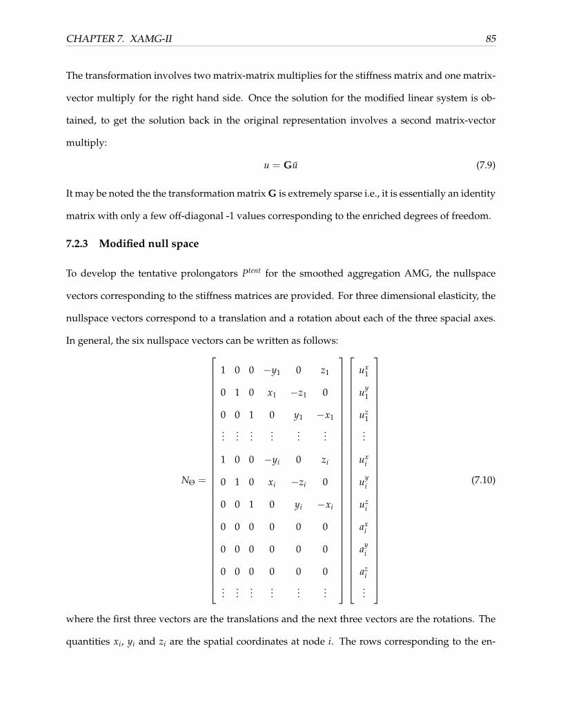
CHAPTER 7. XAMG-II 85
The transformation involves two matrix-matrix multiplies for the stiffness matrix and one matrix-
vector multiply for the right hand side. Once the solution for the modified linear system is ob-
tained, to get the solution back in the original representation involves a second matrix-vector
multiply:
u = Gu (7.9)
It may be noted the the transformation matrix G is extremely sparse i.e., it is essentially an identity
matrix with only a few off-diagonal -1 values corresponding to the enriched degrees of freedom.
7.2.3 Modified null space
To develop the tentative prolongators Ptent for the smoothed aggregation AMG, the nullspace
vectors corresponding to the stiffness matrices are provided. For three dimensional elasticity, the
nullspace vectors correspond to a translation and a rotation about each of the three spacial axes.
In general, the six nullspace vectors can be written as follows:
NΘ =
1 0 0 −y1 0 z1
0 1 0 x1 −z1 0
0 0 1 0 y1 −x1
......
......
......
1 0 0 −yi 0 zi
0 1 0 xi −zi 0
0 0 1 0 yi −xi
0 0 0 0 0 0
0 0 0 0 0 0
0 0 0 0 0 0...
......
......
...
ux1
uy1
uz1
...
uxi
uyi
uzi
axi
ayi
azi
...
(7.10)
where the first three vectors are the translations and the next three vectors are the rotations. The
quantities xi, yi and zi are the spatial coordinates at node i. The rows corresponding to the en-

CHAPTER 7. XAMG-II 86
riched degrees of freedom are all zero since they do not correspond to physical displacements.
In the current approach, even the nullspace vectors need to be transformed to the phantom node
representation. This is done through the following operation:
NΘ = G−1NΘ (7.11)
It may be noted that this operation is not very expensive because of the block-diagonal nature and
extreme sparsity of the transformation matrix. The 2×2 blocks containing the off-diagonal -1 term
can be inverted very inexpensively.
7.3 Implementation
Both serial and parallel implementations of XFEM and AMG routines have been developed. The
XFEM routines are implemented in the finite element program FEAP [65]. ParFEAP is the MPI based
parallel implementation of the program and the XFEM user element routines are also developed
in a manner amenable to parallelization. FEAP comes by default with an interface to PETSC [2]
for the use of many solver routines. The AMG based solution schemes are developed on the
Trilinos [28] platform through a user-solve interface for FEAP. Trilinos is family of numerical
packages developed by Sandia National Laboratories. A new solver class of libraries called XICE
is developed and it interfaces with FEAP and calls the relevant Trilinos packages.
The Trilinos package ML provides the AMG routines for the preconditioners while AztecOO
provides the interface to the conjugate gradient implementation. The global stiffness matrix is
developed on Trilinos as an Epetra CrsMatrix. In the serial implementation, the assembly is
performed directly in FEAP and the global stiffness matrix is passed on to a Trilinos Epetra Crs-
Matrix in directly in terms of compressed sparse row format. In the parallel implementation, the
stiffness matrix assembly is performed within each processor.

CHAPTER 7. XAMG-II 87
7.4 Numerical Results
In this section, some numerical results are presented that compare the computational time and
effort in different solvers.
7.4.1 Linear elastic solves in serial
In Table 7.1, a comparison of different solvers for linear elastic solves in serial is provided. Nine
different cases are considered. Case 1 corresponds to a non-XFEM case and the rest involve XFEM
systems. Figures 7.5 through ?? show some sample cases considered. Case 1 and 2 use the same
mesh with the only difference being that case 1 does not have a crack and is therefore a non-
XFEM example wheras the rest of the examples consider XFEM systems with different mesh sizes
and crack configurations. The column “Direct” corresponds to the case of a direct solver. The
Amesos package of Trilinos was used to provide an interface to the KLU algorithm that first
provides a factorization of the matrix (which takes the most effort) and then solves the linear
system (relatively faster compared to factorization). For this solver, only the CPU time in seconds
is shown.
The other columns correspond to iterative solvers and both the CPU time and the number of
iterations are mentioned. All the iterative solves use the conjugate gradient method. The column
“CG-brute” corresponds to the case where no preconditoner is used. The columns AMG-S1 and
AMG-S5 correspond to the conjugate gradient using a “black-box” AMG preconditioner. S1 and S5
refer to the number of pre- and post- smoother sweeps in the AMG preconditioner. The columns
XAMG-S1 and XAMG-S5 correspond to the proposed AMG scheme involving the phantom node
transformation. Even in this case, the number of pre- and post- sweeps of the smoother is varied.
For both of these preconditioning schemes, a symmetric block Gauss-Seidel smoother was used.
The number of iterations to reduce the residual norm (relative to the initial state) by a factor of
1e-8 is reported.
It is clear from the results that XAMG preconditioning provides the fastest and most efficient
convergence both in terms of CPU time and in terms of the number of Krylov iterations. The num-

CHAPTER 7. XAMG-II 88
(a) Case 2 (b) Case 2 σvm
(c) Case 4 (d) Case 4 σvm
(e) Case 8 σvm
Figure 7.5: Representative examples. Tip enrichments are not used in any of the examples shown.Stress contours correspond to Von Mises stress.
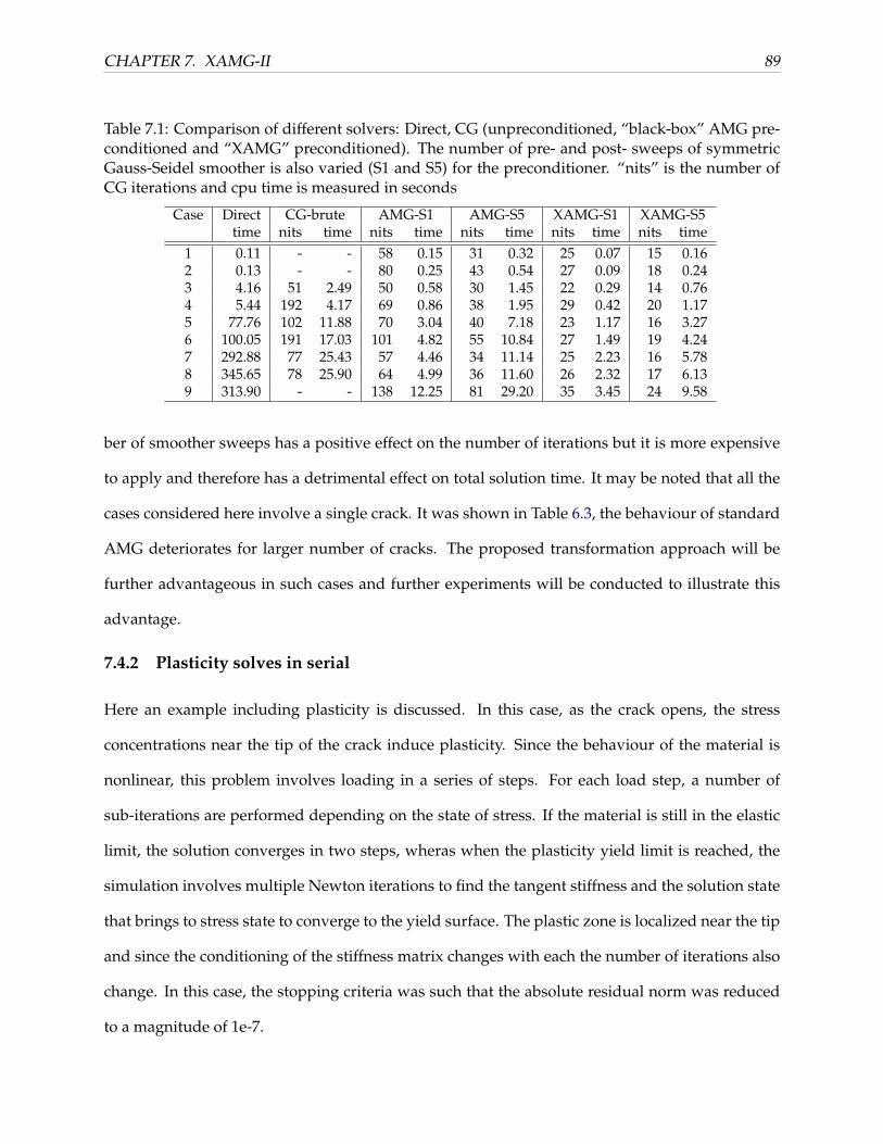
CHAPTER 7. XAMG-II 89
Table 7.1: Comparison of different solvers: Direct, CG (unpreconditioned, “black-box” AMG pre-conditioned and “XAMG” preconditioned). The number of pre- and post- sweeps of symmetricGauss-Seidel smoother is also varied (S1 and S5) for the preconditioner. “nits” is the number ofCG iterations and cpu time is measured in seconds
Case Direct CG-brute AMG-S1 AMG-S5 XAMG-S1 XAMG-S5time nits time nits time nits time nits time nits time
1 0.11 - - 58 0.15 31 0.32 25 0.07 15 0.162 0.13 - - 80 0.25 43 0.54 27 0.09 18 0.243 4.16 51 2.49 50 0.58 30 1.45 22 0.29 14 0.764 5.44 192 4.17 69 0.86 38 1.95 29 0.42 20 1.175 77.76 102 11.88 70 3.04 40 7.18 23 1.17 16 3.276 100.05 191 17.03 101 4.82 55 10.84 27 1.49 19 4.247 292.88 77 25.43 57 4.46 34 11.14 25 2.23 16 5.788 345.65 78 25.90 64 4.99 36 11.60 26 2.32 17 6.139 313.90 - - 138 12.25 81 29.20 35 3.45 24 9.58
ber of smoother sweeps has a positive effect on the number of iterations but it is more expensive
to apply and therefore has a detrimental effect on total solution time. It may be noted that all the
cases considered here involve a single crack. It was shown in Table 6.3, the behaviour of standard
AMG deteriorates for larger number of cracks. The proposed transformation approach will be
further advantageous in such cases and further experiments will be conducted to illustrate this
advantage.
7.4.2 Plasticity solves in serial
Here an example including plasticity is discussed. In this case, as the crack opens, the stress
concentrations near the tip of the crack induce plasticity. Since the behaviour of the material is
nonlinear, this problem involves loading in a series of steps. For each load step, a number of
sub-iterations are performed depending on the state of stress. If the material is still in the elastic
limit, the solution converges in two steps, wheras when the plasticity yield limit is reached, the
simulation involves multiple Newton iterations to find the tangent stiffness and the solution state
that brings to stress state to converge to the yield surface. The plastic zone is localized near the tip
and since the conditioning of the stiffness matrix changes with each the number of iterations also
change. In this case, the stopping criteria was such that the absolute residual norm was reduced
to a magnitude of 1e-7.

CHAPTER 7. XAMG-II 90
Table 7.2 shows the results using the conjugate gradient method without any preconditioner.
The column “plits” indicates the number of Newton iteration subsolves required for convergence
to be achieved. Each Newton iteration corresponds to a number of AMG iterations where the ma-
terial tangent stifnness is updated. The column “cumits” refer to to the cumulative total number
of AMG iterations for that particular load step. In this case, the CG was limited to a maximum of
500 iterations and in many cases even though the sub-solve iterations did not converge, the ap-
proximate solution was sufficient for the Newton method to update the stiffness. Table 7.3 show
the results using a “black-box” AMG preconditioner and Table 7.4 shows the results using the
AMG preconditioner on the transformed XFEM linear system. Similar to the elastic case, the re-
sults show that transformation of the linear system to the phantom node representation greatly
enhances the effectiveness of the AMG preconditioner. Typically for amg-preconditioned iterative
solves, the computational time scales proportionally with the number of iterations. This is not
observed from comparing Tables 7.3 and 7.4 indicating scope for further profiling and code opti-
mization. This effort is currently in progress and it is expected that the reported computational
time results for the transformed system will be revised and the relative advantage of the proposed
approach would be better demonstrated.
Figure 7.6: Simulation involving plasticity: Von Mises stress contours

CHAPTER 7. XAMG-II 91
Table 7.2: Solution of a fracture problem involving plasticity using CG-brute
Load # Iterations Residual norm Energy Norm CPU Timestep plits cumits Initial Final Initial Final (seconds)
1 3 501 8.94E+00 5.28E-08 1.36E-02 0.00E+00 7.202 3 501 8.94E+00 5.28E-08 1.36E-02 0.00E+00 14.173 3 501 8.94E+00 5.28E-08 1.36E-02 0.00E+00 21.154 3 501 8.94E+00 5.28E-08 1.36E-02 0.00E+00 28.135 4 1006 8.94E+00 7.77E-08 1.36E-02 0.00E+00 39.076 10 1445 8.94E+00 3.00E-08 1.36E-02 0.00E+00 60.967 10 1767 8.94E+00 8.90E-08 1.36E-02 0.00E+00 84.538 12 3582 8.95E+00 6.22E-08 1.36E-02 0.00E+00 120.179 24 3181 8.94E+00 1.95E-07 1.36E-02 6.69E-19 171.29
10 26 3654 8.95E+00 2.55E-07 1.36E-02 1.14E-18 227.72
Table 7.3: Solution of a fracture problem involving plasticity using “black-box” AMG-S1
Load # Iterations Residual norm Energy Norm CPU Timestep plits cumits Initial Final Initial Final (seconds)
1 2 77 8.94E+00 1.06E-07 1.36E-02 1.79E-19 2.262 2 77 8.94E+00 1.06E-07 1.36E-02 1.78E-19 4.303 2 77 8.94E+00 1.06E-07 1.36E-02 1.79E-19 6.334 2 77 8.94E+00 1.06E-07 1.36E-02 1.79E-19 8.365 4 153 8.94E+00 9.86E-08 1.36E-02 0.00E+00 12.346 10 475 8.94E+00 7.09E-08 1.36E-02 0.00E+00 22.907 10 499 8.94E+00 1.14E-07 1.36E-02 1.20E-19 33.648 12 665 8.95E+00 9.35E-08 1.36E-02 0.00E+00 47.019 24 774 8.94E+00 2.29E-07 1.36E-02 5.74E-19 69.52
10 26 921 8.95E+00 2.89E-07 1.36E-02 1.07E-18 94.57
Table 7.4: Solution of a fracture problem involving plasticity using XAMG-S1
Load # Iterations Residual norm Energy Norm CPU Timestep plits cumits Initial Final Initial Final (seconds)
1 2 31 8.94E+00 8.53E-08 1.36E-02 0.00E+00 2.232 2 31 8.94E+00 8.70E-08 1.36E-02 0.00E+00 4.203 2 31 8.94E+00 8.90E-08 1.36E-02 0.00E+00 6.154 2 31 8.94E+00 8.71E-08 1.36E-02 0.00E+00 8.115 4 59 8.94E+00 8.86E-08 1.36E-02 0.00E+00 11.946 10 183 8.94E+00 4.11E-08 1.36E-02 0.00E+00 21.667 10 192 8.94E+00 1.17E-07 1.36E-02 1.18E-19 31.448 12 251 8.95E+00 7.21E-08 1.36E-02 0.00E+00 43.359 23 306 8.94E+00 3.35E-07 1.36E-02 1.36E-18 64.70
10 26 357 8.95E+00 2.94E-07 1.36E-02 9.89E-19 88.93

CHAPTER 7. XAMG-II 92
7.5 Summary and Conclusions
In this chapter, a new method to adapt AMG for linear systems arising from modeling fracture
problems using XFEM is discussed. This method involves a simple transformation to an equiv-
alent phantom node representation. Some implementation aspects have been discussed and the
efficacy of this method has been demonstrated on a few numerical examples.

Part IV
Conclusions

CHAPTER 8. SUMMARY 94
Chapter 8
Summary
8.1 Main Contributions
The author’s main contributions in the field of computational modeling of discontinuities in solids
presented in this dissertation are summarized here:
i. XFEM for Inclusions: The extended finite element method is adapted to model multiple
elliptical inclusions within a single element domain. A new and simple formulation for the
enrichment function suitable for elliptical shaped inclusions is presented.
ii. XFEM - Monte Carlo: The extended finite element method is coupled with a Monte Carlo
approach to quantify the uncertainty in the homogenized effective elastic properties of mul-
tiphase materials having random microstructures. The methodology allows for an arbitrary
number, aspect ratio, location and orientation of elliptic inclusions within a matrix, without
the need for fine meshes in the vicinity of tightly packed inclusions and especially without
the need to remesh for every different generated realization of the microstructure. More-
over, the number of degrees of freedom in the enriched elements is dynamically reallocated
for each Monte Carlo sample run based on the given volume fraction. The main advantage
of the proposed XFEM-based methodology is a major reduction in the computational ef-
fort in extensive Monte Carlo simulations compared to the standard FEM approach. Monte
Carlo and XFEM appear to work extremely efficiently together.
iii. XFEM for Cracks: The extended finite element method for modeling both two and three
CHAPTER 8. SUMMARY 95
dimensional cracks is implemented. Further a parallel implementation of the three dimen-
sional crack problem involving general nonlinear material properties has been implemented.
A Trilinos interface to the finite element program FEAP has been developed.
iv. AMG for XFEM - I: It is shown the the linear systems arising from the discretization of frac-
ture mechanics problems using the XFEM are not suitable for a “black-box” application of
AMG. A new quasi-algebraic multigrid method is proposed that is suitable for the linear
systems associated with modeling fracture via extended finite elements. The new method
follows naturally from an energy minimizing algebraic multigrid framework. The key idea
is the modification of the prolongator sparsity pattern to prevent interpolation across cracks.
Numerical experiments have been presented to illustrate that the resulting method con-
verges in a fashion that is relatively insensitive to mesh resolution and to the number of
cracks or their location.
v. AMG for XFEM - II: An alternative method to improve the convergence properties for AMG
applied to XFEM systems that does require invasive modifications to the AMG has been
presented. Here the XFEM system is transformed into an alternate phantom-node repre-
sentation that makes it more suitable for a direct application of AMG. This transformation
automatically decouples the graph of the global stiffness matrix across strong discontinu-
ities ensuring their accurate representation in the multigrid hierarchy. Numerical examples
involving linear and nonlinear materials and implementations in serial and parallel are pre-
sented.
vi. Collaborative contributions: The appendices that follow detail two collaborative efforts that
the author has been involved in. The first effort pertains to the development of a Schwarz
domain decomposition method that allows the AMG method to be applied to fracture me-
chanics simulations while preserving its optimal convergence properties. The second collab-
orative effort involves the use of XFEM coupled with genetic algorithms for flaw detection
in structures.
BIBLIOGRAPHY 96
Bibliography
[1] A. M. Aragon, C. A. Duarte, and P. H. Geubelle. Generalized finite element enrichment
functions for discontinuous gradient fields. International Journal for Numerical Methods in En-
gineering, 82:242–268, 2010.
[2] S. Balay, J. Brown, K. Buschelman, W. D. Gropp, D. Kaushik, M. G. Knepley, L. C. McInnes,
B. F. Smith, and H. Zhang. PETSc Web page, 2011. http://www.mcs.anl.gov/petsc.
[3] S. C. Baxter and L. L. Graham. Characterization of random composites using the moving-
window technique. Journal of Engineering Mechanics, 126(4):389–397, 2000.
[4] T. Belytschko and T. Black. Elastic crack growth in finite elements with minimal remeshing.
International Journal for Numerical Methods in Engineering, 45:601–620, 1999.
[5] T. Belytschko, R. Gracie, and G. Ventura. A review of extended/generalized finite element
methods for mechanics. Modelling and Simulation in Materials Science and Engineering, 17(4),
2009.
[6] T. Belytschko, R. Gracie, and G. Ventura. A review of extended/generalized finite element
models for material modeling. Modeling and Simulation in Materials Science and Engineering,
17:1–24, 2009.
[7] T. Belytschko, N. Moes, S. Usui, and C. Parimi. Arbitrary discontinuities in finite elements.
International Journal for Numerical Methods in Engineering, 50:993–1013, 2001.

BIBLIOGRAPHY 97
[8] L. Berger-Vergiat, H. Waisman, B. Hiriyur, R. Tuminaro, and D. Keyes. Inexact schwarz-
algebraic multigrid preconditioners for crack problems modeled by extended finite element
methods. International Journal for Numerical Methods in Engineering, 2011.
[9] R. I. Borja. Assumed enhanced strain and the extended finite element methods: A unification
of concepts. Computer methods in applied mechanics and engineering, 197:2789–2803, 2008.
[10] A. Brandt. Multigrid techniques: 1984 guide with applications to fluid dynamics. Technical
Report Nr. 85, GMD-Studie, Sankt Augustin, West Germany, 1984.
[11] A. Brandt. General highly accurate algebraic coarsening. Electronic Trans. Num. Anal, 10:1–20,
2000.
[12] A. Brandt. Multiscale scientific computation: Review 2001. In Multiscale and Multiresolution
Methods, pages 1–96. Springer Verlag, 2001.
[13] J. Brannick and L. Zikatanov. Algebraic multigrid methods based on compatible relaxation
and energy minimization. In O. Widlund and D. E. Keyes, editors, Domain Decomposition
Methods in Science and Engineering XVI, volume 55 of Lecture Notes in Computational Science
and Engineering, pages 15–26. Springer, Berlin, 2007.
[14] W. L. Briggs, V. E. Henson, and S. McCormick. A Multigrid Tutorial, Second Edition. SIAM,
Philadelphia, 2000.
[15] L. M. Carvalho, L. Giraud, and P. L. Tallec. Algebraic two-level preconditioners for the Schur
complement method. SIAM J. Scientific Computing, 22:200–1, 1998.
[16] E. N. Chatzi, B. Hiriyur, H. Waisman, and A. W. Smyth. Experimental application and en-
hancement of the xfemga algorithm for the detection of flaws in structures. Computers &
Structures, 89(78):556 – 570, 2011.

BIBLIOGRAPHY 98
[17] D. Cho and L. Zikatanov. A multilevel preconditioning for generalized finite element method
problems on unstructured simplicial meshes. Journal of Numerical Mathematics, 15(3):163–180,
2007.
[18] R. M. Christensen. Asymptotic modulus results for composites containing randomly oriented
fibers. International Journal of Solids and Structures, 12:537–544, 1976.
[19] C. Daux, N. Moes, J. Dolbow, N. Sukumar, and T. Belytschko. Arbitrary cracks and holes with
the extended finite element method. International Journal for Numerical Methods in Engineering,
48:17411760, 2000.
[20] J. D. Eshelby. The determination of the elastic field of an ellipsoidal inclusion, and related
problems. Proceedings of the Royal Society of London. Series A, Mathematical and Physical Sciences,
241(1226):376–396, 1957.
[21] G. E. Fair, R. S. Hay, and E. E. Boakye. Precipitation coating of monazite on woven ceramic
fibers: II. effect of processing conditions on coating morphology and strength retention of
Nextel 610 and 720 fibers. Journal of the American Ceramic Society, 91(5):1508–1516, 2008.
[22] J. Fish. Multiscale computations: Boom or bust. IACM Expressions, 22, 2008.
[23] J. Fish, Q. Yu, and K. Shek. Computational damage mechanics for composite materials based
on mathematical homogenization. International Journal for Numerical Methods in Engineering,
45(11):1657–1679, 1999.
[24] B. Ganapathysubramanian and N. Zabaras. Modeling multiscale diffusion processes in ran-
dom heterogeneous media. Computer Methods in Applied Mechanics and Engineering, 197(43-
44):3560 – 3573, 2008.
[25] A. Gerstenberger and R. Tuminaro. An algebraic multigrid approach to solve xfem based
fracture problems. International Journal for Numerical Methods in Engineering, 2012. submitted.

BIBLIOGRAPHY 99
[26] W. Hackbusch. Multigrid Methods and Applications, volume 4 of Computational Mathematics.
Springer–Verlag, Berlin, 1985.
[27] A. Hansbo and P. Hansbo. A finite element method for the simulation of strong and weak
discontinuities in solid mechanics. Computer Methods in Applied Mechanics and Engineering,
193:3523–3540, 2004.
[28] M. Heroux, R. Bartlett, V. Howle, R. Hoekstra, J. Hu, T. Kolda, R. Lehoucq, K. Long,
R. Pawlowski, E. Phipps, A. Salinger, H. Thornquist, R. Tuminaro, J. Willenbring, A. Williams,
and K. Stanley. An overview of the Trilinos project. ACM Transactions on Mathematical Soft-
ware, 31(3):397–423, September 2005.
[29] R. Hill. The elastic behaviour of a crystalline aggregate. Proceedings of the Physical Society.
Section A, 65(5):349, 1952.
[30] B. Hiriyur, R. Tuminaro, H. Waisman, E. Boman, and D. Keyes. A quasi-algebraic multigrid
approach to fracture problems based on extended finite elements. SIAM Journal on Scientific
Computing, 34(2):A603–A626, 2012.
[31] B. Hiriyur, H. Waisman, and G. Deodatis. Uncertainty quantification in homogenization of
heterogeneous microstructures modeled by xfem. International Journal for Numerical Methods
in Engineering, 88(3):257–278, 2011.
[32] B. L. Karihaloo and Q. Z. Xiao. Modelling of stationary and growing cracks in fe framework
without remeshing: a state-of-the-art review. Computers & Structures, 81(3):119 – 129, 2003.
[33] D. Keyes and W. Gropp. A comparison of domain decomposition techniques for elliptic
partial differential equations and their parallel implementation. SIAM Journal on Scientific
and Statistical Computing, 8:s166–s202, 1987.
[34] T. V. Kolev and P. S. Vassilevski. AMG by element agglomeration and constrained energy
minimization interpolation. Numer. Linear Algebra Appl., 13(9):771–788, 2006.

BIBLIOGRAPHY 100
[35] M. G. Kulkarni, P. H. Geubelle, and K. Matous. Multi-scale modeling of heterogeneous ad-
hesives: Effect of particle decohesion. Mechanics of Materials, 41(5):573 – 583, 2009.
[36] S. Loehnert. Computational homogenization of microheterogeneous materials at finite strains includ-
ing damage. PhD thesis, University Hannover, 2004.
[37] S. Loehnert and T. Belytschko. A multiscale projection method for macro/microcrack simu-
lations. International Journal for Numerical Methods in Engineering, 71(12):1466–1482, 2007.
[38] S. Loehnert and P. Wriggers. Effective behaviour of elastic heterogeneous thin structures at
finite deformations. Computational Mechanics, 41(4):595–606, 2008.
[39] J. Ma, I. Temizer, and P. Wriggers. Random homogenization analysis in linear elasticity based
on analytical bounds and estimates. International Journal of Solids and Structures, In Press,
Accepted Manuscript:–, 2010.
[40] F. Maggi, S. Stafford, T. Jackson, and J. Buckmaster. Nature of packs used in propellant mod-
eling. Physical Review E, 77, 2008.
[41] J. Mandel, M. Brezina, and P. Vanek. Energy optimization of algebraic multigrid bases. Com-
puting, 62:205–228, 1999.
[42] K. Matous. Damage evolution in particulate composite materials. International Journal of
Solids and Structures, 40(6):1489 – 1503, 2003.
[43] S. McCormick and J. Ruge. Multigrid methods for variational problems. SIAM J. on Numerical
Analysis, 19(5):924–929, 1982.
[44] J. M. Melenk and I. Babuska. The partition of unity finite element method: Basic theory and
applications. Computer methods in applied mechanics and engineering, 139:289–314, 1996.
[45] A. Menk and S. Bordas. A robust preconditioning technique for the extended finite element
method. International Journal for Numerical Methods in Engineering, 85(13):1609–1632, 2011.

BIBLIOGRAPHY 101
[46] N. Moes, J. Dolbow, and T. Belytschko. A finite element method for crack growth without
remeshing. International Journal for Numerical Methods in Engineering, 46:131–150, 1999.
[47] S. Mohammadi. Extended finite element method for fracture analysis of structures. Blackwell
Publishing Ltd., 2008.
[48] T. Mori and K. Tanaka. Average stress in matrix and average elastic energy of materials with
misfitting inclusions. Acta Metallurgica, 21(5):571–574, 1973.
[49] S. Natarajan, D. R. Mahapatra, and S. P. A. Bordas. Integrating strong and weak disconti-
nuities without integration subcells and example applications in an xfem/gfem framework.
International Journal for Numerical Methods in Engineering, 83:269–294, 2010.
[50] A. Nouy, A. Clment, F. Schoefs, and N. Mos. An extended stochastic finite element method
for solving stochastic partial differential equations on random domains. Computer Methods in
Applied Mechanics and Engineering, 197(51-52):4663 – 4682, 2008.
[51] L. N. Olson, J. Schroder, and R. S. Tuminaro. A general interpolation strategy for algebraic
multigrid using energy-minimization. submitted to J. Comp. Phys., 2010.
[52] C. Oskay and J. Fish. Eigendeformation-based reduced order homogenization for failure
analysis of heterogeneous materials. Computer Methods in Applied Mechanics and Engineering,
196(7):1216 – 1243, 2007.
[53] C. Oskay and G. Pal. A Multiscale Failure Model for Analysis of Thin Heterogeneous Plates.
International Journal of Damage Mechanics, 19:575–610, 2009.
[54] D. Rabinovich, D. Givoli, and S. Vigdergauz. Crack identification by ’arrival timer’ using
xfem and a genetic algorithm. International Journal for Numerical Methods in Engineering,
77(3):337–359, 2007.
[55] J. Rannou, A. Gravouil, and A. Combescure. A multigrid extended finite element method for
elastic crack growth simulation. European J. of Comp. Mech., 16:161–182, 2007.

BIBLIOGRAPHY 102
[56] A. Reuss. Berechnung der fliegrenze von mischkristallen auf grund der plastizittsbedingung
fr einkristalle. ZAMM - Journal of Applied Mathematics and Mechanics / Zeitschrift fr Angewandte
Mathematik und Mechanik, 9:49–58, 1929.
[57] Z. Shan and A. M. Gokhale. Representative volume element for non-uniform micro-structure.
Computational Materials Science, 24(3):361–379, 2002.
[58] J. Shi, D. Chopp, J. Lua, N. Sukumar, and T. Belytschko. Abaqus implementation of extended
finite element method using a level set representation for three-dimensional fatigue crack
growth and life predictions. Engineering Fracture Mechanics, 77(14):2840 – 2863, 2010.
[59] C. Siefert and E. de Sturler. Probing methods for saddle point problems. Elec. Trans. Numer.
Anal., 22:163–183, 2006.
[60] A. Simone. Partition of unity-based discontinuous elements for interface phenomena: Com-
putational issues. Communications in Numerical Methods in Engineering, 20(6):465–478, 2004.
[61] J. Song, P. Areias, and T. Belytschko. A method for dynamic crack and shear band propaga-
tion with phantom nodes. International Journal for Numerical Methods in Engineering, 67:868893,
2006.
[62] K. R. Srinivasan, K. Matous, and P. H. Geubelle. Generalized finite element method for mod-
eling nearly incompressible bimaterial hyperelastic solids. Computer Methods in Applied Me-
chanics and Engineering, 197:4882–4893, 2008.
[63] N. Sukumar, D. L. Chopp, N. Moes, and T. Belytschko. Modeling holes and inclusions by
level sets in the extended finite-element method. Computer Methods in Applied Mechanics and
Engineering, 190(46-47):6183 – 6200, 2001.
[64] J.-H. S. T. Belytschko, S. Loehnert. Multiscale aggregating discontinuities a method for cir-
cumventing loss of material stability. International Journal for Numerical Methods in Engineering,
73:869–894, 2007.

BIBLIOGRAPHY 103
[65] R. Taylor. FEAP – a finite element analysis program, 2011. http://www.ce.berkeley.edu/
projects/feap/parmanual.pdf.
[66] M. Tootkaboni and L. Graham-Brady. A multi-scale spectral stochastic method for homoge-
nization of multi-phase periodic composites with random material properties. International
Journal of Numerical Methods in Engineering, 2009.
[67] S. Torquato. Random heterogeneous materials: microstructure and macroscopic properties. Springer
Science and Business Media Inc., 2001.
[68] A. B. Tran, J. Yvonnet, Q.-C. He, C. Toulemonde, and J. Sanahuja. A multiple level set ap-
proach to prevent numerical artefacts in complex microstructures with nearby inclusions
within xfem. International Journal for Numerical Methods in Engineering, 2010.
[69] U. Trottenberg, C. Oosterlee, and A. Schuller. Multigrid. Academic Press, London, UK, 2001.
[70] R. Tuminaro and C. Tong. Parallel smoothed aggregation multigrid: Aggregation strategies
on massively parallel machines. In J. Donnelley, editor, SuperComputing 2000 Proceedings,
2000.
[71] P. Vanek, M. Brezina, and J. Mandel. Convergence of algebraic multigrid based on smoothed
aggregation. Numerische Mathematik, 88(3):559–579, 2001.
[72] P. Vanek, J. Mandel, and M. Brezina. Algebraic multigrid based on smoothed aggregation for
second and fourth order problems. Computing, 56:179–196, 1996.
[73] P. S. Vassilevski. General constrained energy minimization interpolation mappings for AMG.
SIAM J. Sci. Comput., 32(1):1–13, 2010.
[74] W. Voigt. Lehrbuch der Kristallphysik. B. G. Teubner, Leipzig, 1910.
[75] C. Wagner. On the algebraic construction of multilevel transfer operators. Computing, 65:73–
95, August 2000.

BIBLIOGRAPHY 104
[76] H. Waisman and T. Belytschko. Parametric enrichment adaptivity by the extended finite
element method. International Journal for Numerical Methods in Engineering, 73(12):1671–1692,
2009.
[77] H. Waisman, E. Chatzi, and A. W. Smyth. Detection and quantification of flaws in struc-
tures by the extended finite element method and genetic algorithms. International Journal for
Numerical Methods in Engineering, 2009.
[78] W. L. Wan, T. F. Chan, and B. Smith. An energy-minimizing interpolation for robust multigrid
methods. SIAM J. Sci. Comput., 21(4):1632–1649, 2000.
[79] M. D. Webb and I. L. Davis. Random particle packing with large particle size variations using
reduced dimension algorithms. Powder Technology, 2006.
[80] P. Wriggers. Computational contact mechanics. Wiley, NY, 2002.
[81] J. Xu and L. Zikatanov. On an energy minimizing basis for algebraic multigrid methods.
Computing and Visualization in Science, 7:121–127(7), October 2004.
[82] J. Xu and L. T. Zikatanov. On multigrid methods for generalized finite element methods. In
Meshfree methods for partial differential equations (Bonn, 2001), volume 26 of Lect. Notes Comput.
Sci. Eng., pages 401–418. Springer, Berlin, 2003.
[83] Z. Yuan and J. Fish. Toward realization of computational homogenization in practice. Inter-
national Journal for Numerical Methods in Engineering, 73:361–380, 2008.
[84] H. H. Zhang and L. X. Li. Modeling inclusion problems in viscoelastic materials with the
extended finite element method. Finite Elements in Analysis and Design, 45(10):721 – 729, 2009.
[85] Q. Zhang, M. Zhao, Y. Liu, A. Cao, W. Qian, Y. Lu, and F. Wei. Energy-absorbing hybrid
composites based on alternate carbon-nanotube and inorganic layers. Advanced Materials,
21(28):2876–2880, 2009.

APPENDIX A. XFEM-AMG-DD 105
Appendix A
Schwarz-AMG for XFEM
In this chapter, another algebraic multigrid preconditioner based on the concept of Domain Decomposition and
suitable for fracture problems is presented. This work is reproduced in part from Berger-Vergiat et. al. [8]. Inputs
from the co-authors are gratefully acknowledged.
A.1 Introduction
In this article a simple domain decomposition approach is reproduced that retains the AMG ad-
vantages on well behaved domains by avoiding the coarsening of enriched degrees of freedom.
The idea is to employ a multiplicative Schwarz preconditioner where the physical domain is par-
titioned into a healthy (or unfractured) and cracked subdomains. First, the healthy subdomain
containing only standard degrees of freedom, is solved approximately by one AMG V-cycle, fol-
lowed by concurrent direct solves of cracked subdomains. This strategy alleviates the need to
redesign special AMG coarsening strategies that can handle XFEM discretizations. Numerical
examples on various crack problems clearly illustrate the superior performance of this approach
over a brute force AMG preconditioner applied to the linear system.
In the present work domain decomposition concepts based on the multiplicative Schwarz
method are employed to reformulate the problem so that AMG would retain its convergence
features when applied to the bulk of the domain that contains no cracks. Hence, the problem
is partitioned in a way that separates the enriched degrees of freedom from the nodes that are not
enriched. The formulation and the proposed preconditioner are outlined in the following subsec-

APPENDIX A. XFEM-AMG-DD 106
tions.
A.2 Domain Decomposition formulation for cracks: A multiplicativeSchwarz approach
The proposed multiplicative Schwarz preconditioner begins with a special domain decomposi-
tion. As shown in Fig. A.1, two possible partitioning strategies are considered: (i) a single sub-
domain containing all cracks (see Fig. A.1a) and (ii) multiple crack subdomains (see Fig. A.1b),
where each crack owns its own subdomain. In many cases the physics of the problem will de-
termine the partitioning scheme. For example, clusters of cracks and microcracks, e.g., formed
due to a localized impact or indentation loads, can be aggregated into a single subdomain, while
more isolated cracks, nucleating at far distances from each other, e.g., formed due to fatigue loads
applied to the whole structure, may be too far apart and will require their own subdomains. In
any case, the two strategies lead to the same type of systems.
In Fig. A.1, the subdomain Ωh1 that does not contain any enriched nodes (or cracks) is referred
to as a “healthy” subdomain (for simplicity of the presentation only one healthy subdomain is con-
sidered). The other subdomains containing at least one crack, and hence all enriched degrees
of freedom associated with that crack, are referred to as “cracked” subdomains and denoted by
Ωci . Cracked subdomains may also contain one or several layers of elements around cracks that
constitute the overlap with the healthy subdomain.
The general formulation leads to a coupled set of linear systems associated with the healthy
and cracked subdomains. The coupling occurs through the boundary conditions and overlapping
elements. Note that in this formulation, cracked subdomains are decoupled from each other and
are only coupled to the healthy subdomain. This property is not an essential feature of the pro-
posed approach, but is adopted in the current work to keep the description of the method simple,
without any loss of generality.

APPENDIX A. XFEM-AMG-DD 107
hhhhhhhh
//////////////////
/
Ω1
Ω1
Γ1
Γc
h
c
Γ1
hhhhhhh ///////////
/////
Ω1
Ω1
Ω2
Ω3
h
c
c
c
c
Γ1
Γ
c
Γ3
c
Γ2
h
Γ1
h
(a)
hhhhhhhh
//////////////////
/
Ω1
Ω1
Γ1
Γc
h
c
Γ1
hhhhhhh ///////////
/////
Ω1
Ω1
Ω2
Ω3
h
c
c
c
c
Γ1
Γ
c
Γ3
c
Γ2
h
Γ1
h
(b)
Figure A.1: Schematic representation of the “healthy” and “cracked” subdomains in the formulationof domain decomposition. [a] multiple cracks share a single cracked subdomain [b] each crack isassigned to a different cracked subdomain.
Mathematically, the decomposition into subdomains is written in the following way:
Kh1uh
1 = fh1 in Ωh
1 with uh1 = uE on Γ
and with uh1 = uc
1 on Γcj
Kc1uc
1 = fc1 in Ωc
1 with uc1 = uh
1 on Γc1
Kc2uc
2 = fc2 in Ωc
2 with uc2 = uh
1 on Γc2
...
Kcnuc
n = fcn in Ωc
n with ucn = uh
1 on Γcn
(A.1)
The superscript h is employed to denote an operator or variable defined on a healthy subdomain
and the superscript c denotes operators or variables defined on a cracked subdomain. Note that the
healthy subdomain is solved first, followed by cracked subdomains. Ω = Ωh1 ⊕Ωc
1 ⊕ ...⊕Ωcnc= Ωh
1
nc⊕i=1
Ωci
is the finite element space associated with the problem, nc is the number of cracked subdomains, uE
are the values of the displacement field where essential boundary are imposed, Γ is the boundary
of Ω and Γi is the boundary of subdomain Ωi. The solution over the full problem domain (hence-
forth referred to as global) is formed by assembling the solutions from the subdomain problems.
Once the problem is discretized by finite elements, in each subdomain, the stiffness matrix, force
vector and the unknown displacement vector are denoted by K,f and u, respectively.

APPENDIX A. XFEM-AMG-DD 108
A simple procedure to generate a cracked subdomain employs the levelset formulation and is
described as follows. Start by forming a set which is the union of all elements having specified
overlap for a given crack with the healthy subdomain. This is easily generated by selecting all
the nodes that have levelset values smaller than no × he,where he is the characteristic dimension
of an element. If no is chosen equal to 1, only the elements containing the crack are selected.
Choosing no = 2 selects all elements containing at least one enriched node. This would create
a non-overlapping partition of the domain between cracked subdomains and the healthy subdo-
main, and could be well suited for application of a FETI algorithm. An illustration of the domain
decomposition and the overlapping elements for XFEM are shown in Fig. A.2.
Overlapping elements Overlapping elements
Figure A.2: Two overlapping domains employed in the Schwarz method. The following colorlegend is used: black squares represent Schwarz essential boundary conditions, the black trianglesrepresent clamped nodes, the red circles represent pulled nodes, the green zone represent the ele-ments belonging to the same subdomain, the blue zone represent the elements that are part of theoverlapping layer.
The Schwarz algorithm may be written in the following way. The linear system on subdo-
main i (healthy or cracked) is extracted from the global system by employing a restriction operator
Ri : ΩN×N → ΩNid×N
i , where N denotes the overall number of degrees of freedom and Nid the
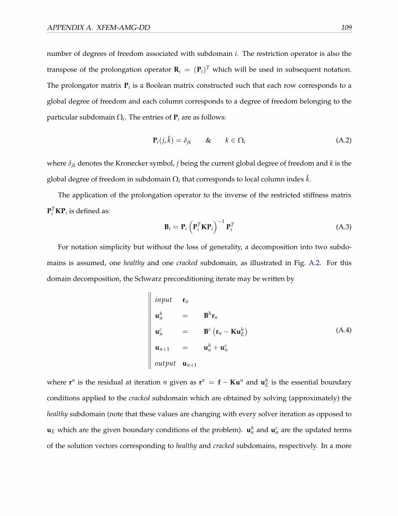
APPENDIX A. XFEM-AMG-DD 109
number of degrees of freedom associated with subdomain i. The restriction operator is also the
transpose of the prolongation operator Ri = (Pi)T which will be used in subsequent notation.
The prolongator matrix Pi is a Boolean matrix constructed such that each row corresponds to a
global degree of freedom and each column corresponds to a degree of freedom belonging to the
particular subdomain Ωi. The entries of Pi are as follows:
Pi(j, k) = δjk & k ∈ Ωi (A.2)
where δjk denotes the Kronecker symbol, j being the current global degree of freedom and k is the
global degree of freedom in subdomain Ωi that corresponds to local column index k.
The application of the prolongation operator to the inverse of the restricted stiffness matrix
PTi KPi is defined as:
Bi = Pi
(PT
i KPi
)−1PT
i (A.3)
For notation simplicity but without the loss of generality, a decomposition into two subdo-
mains is assumed, one healthy and one cracked subdomain, as illustrated in Fig. A.2. For this
domain decomposition, the Schwarz preconditioning iterate may be written by∥∥∥∥∥∥∥∥∥∥∥∥∥∥∥∥∥∥
input rn
uhn = Bhrn
ucn = Bc (rn −Kuh
E)
un+1 = uhn + uc
n
output un+1
(A.4)
where rn is the residual at iteration n given as rn = f − Kun and uhE is the essential boundary
conditions applied to the cracked subdomain which are obtained by solving (approximately) the
healthy subdomain (note that these values are changing with every solver iteration as opposed to
uE which are the given boundary conditions of the problem). uhn and uc
n are the updated terms
of the solution vectors corresponding to healthy and cracked subdomains, respectively. In a more

APPENDIX A. XFEM-AMG-DD 110
compact notation, Eq. (A.4) becomes:
un+1 =(
Bh + Bc − BcKBh)
rn = Mrn (A.5)
Where M is the preconditioning operator. Note that M defined in Eq. (A.5) is not symmetric. One
could symmetrize the preconditioner by adding an additional solve of cracked subdomains before
the healthy part, as follows: ∥∥∥∥∥∥∥∥∥∥∥∥∥∥∥∥∥∥∥∥∥∥
input rn
uc1n = Bcrn
uhn = Bh (rn −Kuc1
E)
uc2n = Bc (rn −Kuh
E)
un+1 = uc1n + uh
n + uc2n
output un+1
(A.6)
In a compact matrix form it reads:
Msym = Bc + Bh − BhKBc − BcKBh + BcKBhKBc (A.7)
= Bc + (I− BcK)Bh (I−KBc) (A.8)
Normally, a symmetric form of the preconditioner allows for a bigger choice of iterative solvers.
However, it also must be noted that it requires the application of the operator Bc twice, which is
more expensive, and hence is not be pursued in this work.
Another way of creating a symmetric system is to use an additive Schwarz algorithm instead
of a multiplicative one. The idea of the additive Schwarz algorithm is to solve all subdomains
concurrently. In contrast with the multiplicative Schwarz approach, the non symmetric term in
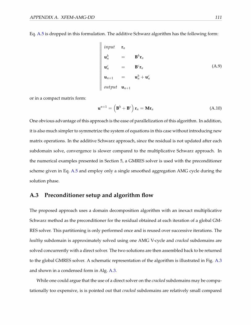
APPENDIX A. XFEM-AMG-DD 111
Eq. A.5 is dropped in this formulation. The additive Schwarz algorithm has the following form:∥∥∥∥∥∥∥∥∥∥∥∥∥∥∥∥∥∥
input rn
uhn = Bhrn
ucn = Bcrn
un+1 = uhn + uc
n
output un+1
(A.9)
or in a compact matrix form:
un+1 =(
Bh + Bc)
rn = Mrn (A.10)
One obvious advantage of this approach is the ease of parallelization of this algorithm. In addition,
it is also much simpler to symmetrize the system of equations in this case without introducing new
matrix operations. In the additive Schwarz approach, since the residual is not updated after each
subdomain solve, convergence is slower compared to the multiplicative Schwarz approach. In
the numerical examples presented in Section 5, a GMRES solver is used with the preconditioner
scheme given in Eq. A.5 and employ only a single smoothed aggregation AMG cycle during the
solution phase.
A.3 Preconditioner setup and algorithm flow
The proposed approach uses a domain decomposition algorithm with an inexact multiplicative
Schwarz method as the preconditioner for the residual obtained at each iteration of a global GM-
RES solver. This partitioning is only performed once and is reused over successive iterations. The
healthy subdomain is approximately solved using one AMG V-cycle and cracked subdomains are
solved concurrently with a direct solver. The two solutions are then assembled back to be returned
to the global GMRES solver. A schematic representation of the algorithm is illustrated in Fig. A.3
and shown in a condensed form in Alg. A.3.
While one could argue that the use of a direct solver on the cracked subdomains may be compu-
tationally too expensive, is is pointed out that cracked subdomains are relatively small compared

APPENDIX A. XFEM-AMG-DD 112
Exact Solves on cracked domains
Inexact AMG solve on Ωh
Ω1c
Ω2c
Ω3c
Ωnc
GMRES
Figure A.3: Schematic description of the inexact Schwarz-AMG preconditioner .
to the overall size of the problem and therefore, this step is fairly inexpensive. Moreover, lin-
ear systems associated with cracked subdomains are factored before starting GMRES iterations,
and reused in successive iterations of the preconditioner. Nonetheless in the case of propagating
cracks, a new partition may need to be built at every crack propagation step. Hence, the linear sys-
tems associated with cracked subdomains must also be re-factored after each crack propagation
step.
Algorithm A.3.1 GMRES preconditioned by an inexact Schwarz-AMG preconditionerStep 1: Apply one AMG V cycle to the healthy subdomain
uh ← AMG(rh, Kh) for the healthy subdomain
Step 2: solve all cracked subdomains
uci ← Bi(rh −Khuh) for all cracked subdomains i
Step 3: Update the residual and return to the GMRES solver
u← assemble(uh, uc1, . . . , uc
n)

APPENDIX A. XFEM-AMG-DD 113
A.4 Representative Example
A.4.1 Multiple cracks with different lengths and orientations
In this example the convergence of the preconditioners on a plate containing three cracks of dif-
ferent lengths and orientations is investigated. Two strategies, illustrated in Fig. A.1, are used to
partition the domain into healthy and cracked subdomains. In the first case the cracked subdomain
owns all the cracks (a single cracked subdomain) while in the second approach each crack owns its
own local subdomain (multiple cracked subdomains). In addition an Additive Schwarz method is
investigated and compared with the other methods. The mesh and the partitioned domains are
shown in Fig. A.4, and the convergence results are plotted in Fig. A.5.
0 0.1 0.2 0.3 0.4 0.5 0.6 0.7 0.8 0.9 10
0.1
0.2
0.3
0.4
0.5
0.6
0.7
0.8
0.9
1
Student Version of MATLAB
(a)0 0.1 0.2 0.3 0.4 0.5 0.6 0.7 0.8 0.9 1
0
0.1
0.2
0.3
0.4
0.5
0.6
0.7
0.8
0.9
1
Student Version of MATLAB
(b)
Figure A.4: Domain decomposition and mesh of a plate with three cracks with different lengthsand orientations [a] Decomposition with multiple cracked subdomains [b] Decomposition with asingle cracked subdomain.
It is clear that both domain decomposition strategies give excellent results compared to the AMG
brute force preconditioner. The AMG performance is poor, which is mainly attributed to the cracks
having two sets of tip functions inside the domain, and in close proximity to each other. More-
over, the different orientation of the cracks makes it significantly harder for the AMG to generate

APPENDIX A. XFEM-AMG-DD 114
0 20 40 60 80 100 120 140 160 180 20010−16
10−14
10−12
10−10
10−8
10−6
10−4
10−2
100
Number of iterations
Nor
m o
f the
resi
dual
AMG brute forceAdditive Schwarz−AMG multipleAdditive Schwarz−AMG singleMultiplicative Schwarz−AMG multipleMultiplicative Schwarz−AMG singleExact Schwarz−AMG multipleExact Schwarz−AMG single
Student Version of MATLAB
Figure A.5: Comparison of the convergence rate for the decomposition strategies shown in Fig.A.4.

APPENDIX A. XFEM-AMG-DD 115
appropriate aggregates and the coarsening of these special functions, significantly deteriorates its
performance.
As expected, the multiplicative inexact Schwarz method with a single cracked subdomain gives
slightly better performance than its counterpart with multiple cracked subdomains. The single
cracked subdomain has converged in 50 iterations whereas it converged in 63 iterations when mul-
tiple subdomains are introduced. This behavior is due to the fact that all the cracks are solved
concurrently in the single cracked subdomain case whereas solving them in a sequential manner
introduce a small delay in the coupling of these cracks. The convergence of the additive Schwarz
method is slightly worse than the multiplicative Schwarz as has been noticed before.
Table A.1: Summary of the convergence results for the problem considered in Fig. A.4.
AMG Additive Multiplicative Exactbrute force Schwarz-AMG Schwarz-AMG Schwarz-AMG
Single ”crack”190 68 50 48
subdomainMultiple ”crack”
190 74 63 59subdomains
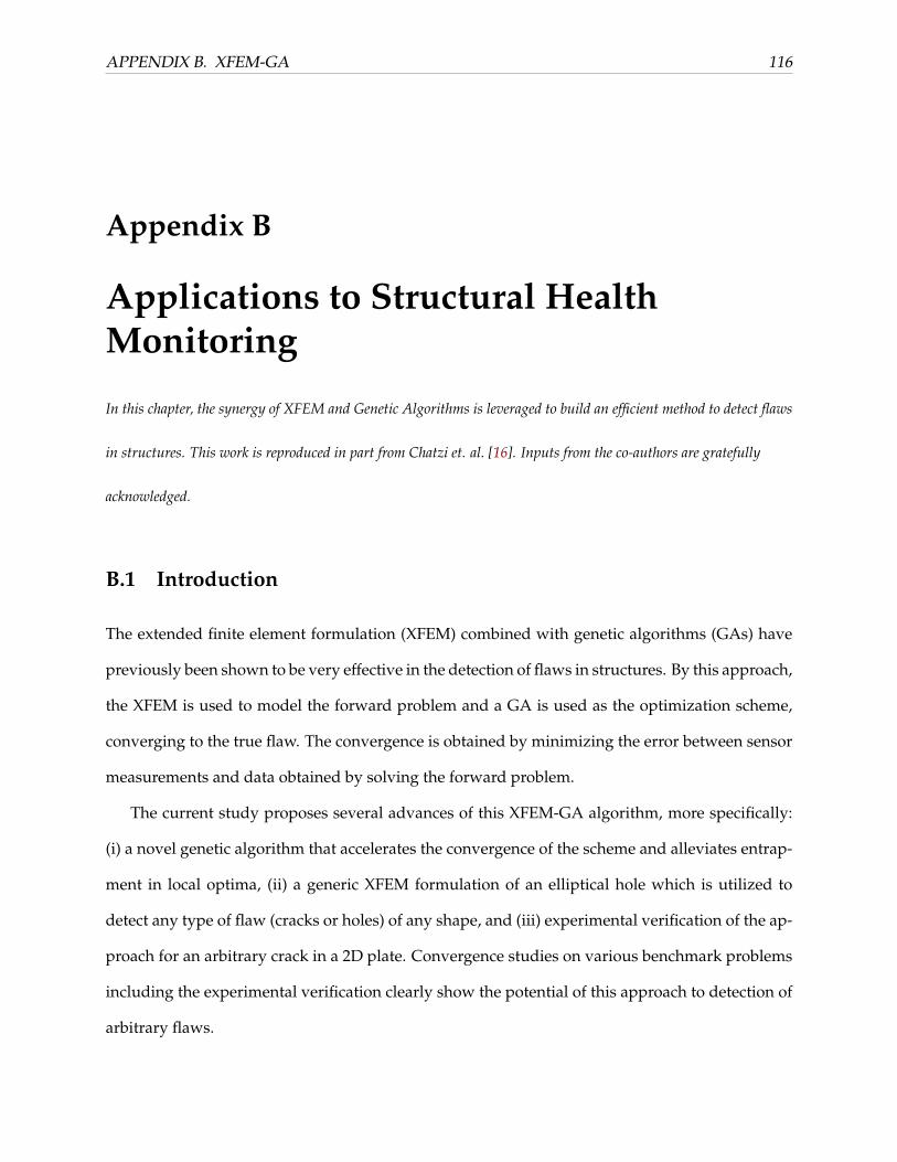
APPENDIX B. XFEM-GA 116
Appendix B
Applications to Structural HealthMonitoring
In this chapter, the synergy of XFEM and Genetic Algorithms is leveraged to build an efficient method to detect flaws
in structures. This work is reproduced in part from Chatzi et. al. [16]. Inputs from the co-authors are gratefully
acknowledged.
B.1 Introduction
The extended finite element formulation (XFEM) combined with genetic algorithms (GAs) have
previously been shown to be very effective in the detection of flaws in structures. By this approach,
the XFEM is used to model the forward problem and a GA is used as the optimization scheme,
converging to the true flaw. The convergence is obtained by minimizing the error between sensor
measurements and data obtained by solving the forward problem.
The current study proposes several advances of this XFEM-GA algorithm, more specifically:
(i) a novel genetic algorithm that accelerates the convergence of the scheme and alleviates entrap-
ment in local optima, (ii) a generic XFEM formulation of an elliptical hole which is utilized to
detect any type of flaw (cracks or holes) of any shape, and (iii) experimental verification of the ap-
proach for an arbitrary crack in a 2D plate. Convergence studies on various benchmark problems
including the experimental verification clearly show the potential of this approach to detection of
arbitrary flaws.

APPENDIX B. XFEM-GA 117
B.2 XFEM approach for solution of the forward problem
In XFEM, the effect of internal features such as cracks, voids or material interfaces are captured by
introducing special functions, which locally enrich the span of basis functions in the discretized
system.
The general form of the discretized weak form approximation for the solution variable u(x) in
XFEM is given as follows:
uh(x) = ∑I∈N
NI(x)uI + ∑J∈Nenr
I
(∑I∈F
ΦI(x)aI J
)(B.1)
Here N refers to the all the nodes in the mesh and NenrI refers to the subset of N that contains all
the nodes enriched by the functions ΦI , called the support of the basis ΦI . This support is made
up of only those elements that contain within their domains, the discontinuity interface modeled
by ΦI . If an element-wise discretized weak form is considered, both N and Nenr (for an enriched
element) refer to the number of element nodes Ne. The enrichments are controlled by degrees of
freedom aI J which are additional unknowns to be solved for, in the global system of equations.
When considering XFEM for linear elastic fracture mechanics, the number of enrichment func-
tions F generally equals 1 for elements with a crack interface and the Heavyside step function
H(x) is used for Φ. For elements with a crack-tip, F generally equals 4 and the span of ΦI is suit-
ably chosen to model tip singularity. In the case of XFEM for modeling weak-discontinuities (such
as those caused by material inclusions), a single enrichment function which is C0 continuous is
used. The discretized weak form for an enriched element is given as:
uhe (x) = ∑
I∈Ne
NI(x) (uI + Φ(x)aI) (B.2)
It may be seen from equation B.2 that the physical displacement at an enriched node I is pro-
vided in terms of both the standard dof uI and the enriched dof aI . To ensure that the physical
displacement solution is completely defined by the standard dof uI , a shifted-basis form of equa-
tion (B.2) may be written as follows:

APPENDIX B. XFEM-GA 118
uhe (x) = ∑
I∈Ne
NI(x)(uI +
[Φ(x)− Φ(xI)
]aI)
(B.3)
B.2.1 Convergence of elliptical enrichment
The convergence of the elliptical approximation to the modeling of a straight crack is studied. Fig-
ure B.1(a) represents a rectangular mesh grid with a straight crack shown as a red line, subjected
to load and boundary conditions as shown. An FEM analysis on a mesh conforming to the in-
ternal boundaries with the presence of double nodes along the crack was performed. The results
from this analysis (Displacement solution in Fig. B.1(b)) was used as a benchmark to compare
against the XFEM ellipse approximation. The XFEM approximation involved an ellipse with a
major radius equal to the crack length and oriented in the same direction. The variable parameter
in this study was the ellipse aspect ratio r = minor/major radius, which varied from 1 (circle) to
0.1 (elongated ellipse). As shown in Fig. B.1(c), the norm of the relative error in nodal displace-
ments between the XFEM and FEM analyses shows a linear trend decreasing to substantially low
magnitudes as the ellipse minor radius is reduced. Since the FEM nodes did not overlap with the
XFEM nodes, the FEM nodal displacements were first interpolated to the XFEM node locations
before the error was computed. The results confirm that an ellipse with a sufficiently small aspect
ratio can be used as a good approximation to a crack.
B.3 GA - XFEM based Identification
Genetic Algorithms have been chosen as the optimization tool for this non destructive detec-
tion scheme. GAs have long been used as an efficient tool for search, optimization and machine
learning problems. The main concept associated with this particular method is the mimicking
of the biological processes of natural evolution and survival of the fittest candidates. According
to Holland’s Genetic Algorithm each potential optimal solution to a problem can be seen as an
individual that can be coded by a set of genes. Usually these genes are chosen to be binary bits
and the binary string or alternatively the “individual” is also known as a chromosome. A random

APPENDIX B. XFEM-GA 119
(a) (b)
00.10.20.30.40.50.60.70.80.9110
−3
10−2
10−1
100
r = b/a
|u−
u ex| 2 /
|uex
|
θ = 0
θ = 90
θ = 45
(c)
Figure B.1: Convergence study of crack modeled with elliptical enrichment

APPENDIX B. XFEM-GA 120
generation of such chromosomes provides us with the initial population. At each cycle of the evo-
lutionary process a new set of offsprings is produced from the fittest individuals of the previous
generation. Reproduction takes place through the recombination of the bit strings or simple bit
flips that occur with some probability. The purpose of this evolutionary procedure is to eventually
lead to the survival of the fittest individual, as this will be the one to produce the largest number
of offsprings and thus has the best chances for survival. All genetic algorithms are based on the
following scheme (Figure B.2 - classic GA):
• Representation: Depending on the application the parameters of the problem can be either
integer or real numbers. Usually, the set of parameters can be appropriately encoded into a
finite length binary string. Once a representation is decided a number of different chromo-
somes is randomly generated to form the initial population.
• Fitness Evaluation - Selection: The evaluation of the fitness for each member of the pop-
ulation is carried out through the use of an objective function associated with each prob-
lem. The suitability of each chromosome is the criterion based on which this individual
will be selected for reproduction. Selection can be performed through various schemes like
“roulette wheel” selection or “tournament” selection. The roulette wheel selection is solely
dependent upon the performance (fitness) of each individual. In the case of the second
method, the probability of a string selection is also dependent upon the fitness of the “com-
petitive” strings chosen to participate in a tournament round. The latter contributes toward
the preservation of the diversity of the population.
• Crossover: This operator is applied with a certain probability, to the pairs of the previously
selected individuals (parents). In general the crossover procedure randomly selects a posi-
tion in the binary string and mutually exchanges the parts of the chromosome before and
after this location in order to produce two offsprings.
• Mutation: The use of the crossover procedure as the only means for generating new in-
dividuals could result in the loss of the diversity of the population. This problem can be

APPENDIX B. XFEM-GA 121
overcome using the mutation operator which involves the random flip of the binary genes
of the chromosome for the case of jump mutation, or the alteration of the phenotypic (real)
representation of the design parameters by a small increment or decrement for the case of
creep mutation.
In a nutshell, the basic GA consists of coding each potentially optimal solution to a prob-
lem, as a set of genes. Usually these genes are chosen to be binary bits, and the binary string
or alternatively the “individual”, is also known as a chromosome. Random generation of such
chromosomes provides the initial population. At each cycle of the evolutionary process a new
set of offsprings is produced from the fittest individuals of the previous generation (Selection).
Reproduction takes place through the recombination of the bit strings (Crossover) or simple bit
flips (Mutation) that occur with some probability. The purpose of this evolutionary procedure is
to eventually lead to the survival of the fittest individual, as this will be the one to produce the
largest number of offsprings and thus has the best chances for survival (Figure B.2).
Initial Population
Fitness Evaluation
Optimal Parameters
Start
yes
no
Selection
Crossover
Mutation
Form Next Generation
XFEM run
Are the optimality criteria satisfied?
Parent chromosomes
Children
Figure B.2: The XFEM-GA algorithm flowchart.
In the context of the current work, there are several noted advantages to using genetic algo-
rithms: (i) they have been fairly well studied in the literature and have proven to be very efficient
on difficult optimization problems (converging to a global minima), (ii) the current problem is ex-

APPENDIX B. XFEM-GA 122
tremely difficult as the forward model keeps changing and updating. Hence there is no straight-
forward analytical expression connecting the strain field to the crack parameters which may cause
traditional methods to stagnate, (iii) they are not limited by constraints imposed by other ana-
lytical methods which usually require linear or differentiable objective functions and a proper
estimation of the initial parameter interval, and (iv) can easily be implemented and adjusted to
any user source codes. The problem described in Section 2, consists of finding the parameters de-
scribing the flaw, i.e., for linear cracks-the tip coordinates, for circular holes-the radius and center
coordinates, or for elliptical holes-the center, minor and major axes and orientation angle. This
is achieved through minimizing the residual of the XFEM-GA estimate with respect to the actual
data provided at specific sensor locations, usually along the boundaries (equation (B.4)):
r (βi) =‖εγ (βi)− ε0
γ‖‖ε0
γ‖(B.4)
where ‖ · ‖ denotes the L2 norm, ε0γ is the real measured data (in most cases, this is the mea-
sured strain obtained from the damaged model) at some locations along the surface and εγ are the
computed strains at the exact same points. These computed strains are a function of the optimiza-
tion parameters βi which change with the forward problem as the outer (optimization) iteration
proceeds.
The problem setup involves the definition of the number of unknown parameters as well as the
discretized search space (upper, lower bounds and number of discrete possibilities per parame-
ter). The XFEM-GA identification process is initiated with the generation of binary bit individuals
(chromosomes), which are randomly selected from the search space, serving as the initial popu-
lation. The next step involves the fitness evaluation of each individual in the population group.
The fitness function to be minimized is the one defined in equation (B.4). At the next cycle a new
set of offsprings is produced from the fittest individuals of the previous generation using the tour-
nament selection scheme. The mechanisms of reproduction (mutation and crossover) are applied
and the evolutionary cycle continues for a specific number of total generations.

APPENDIX B. XFEM-GA 123
B.3.1 Applied Weighted Average Mutation GA (WAM-GA)
Most population-based, reproductive, optimization algorithms such as genetic algorithms, ant
colony optimization, and particle swarm optimization (PSO) often deal with the premature con-
vergence problem. This problem occurs when highly fit parents in a population pool rapidly
dominate the breeding process, commonly leading to confinement in local optima. The crossover
operator, is not enough to circumvent this hindrance since it uses only acquired information. The
mutation operator on the other hand, can move into broader areas within the search space in con-
trast to the crossover, but it also can not change many bits in individuals because the mutation
rate is too low. If the mutation rate is set to a high value, then genetic algorithms approach the
global optimum very slowly. As a result, it is very difficult to escape this premature convergence
problem.
This method suggests the use of a guided mutation scheme applied at the phenotype, mean-
ing the real representation of the individual (creep mutations). The standard implementation for
the creep mutation scheme is for a child to differ from its parent by only a small increment or
decrement, usually toward a random direction. The novel Weighted Average Mutation (WAM-
GA) implemented here, takes advantage of the large amount of information obtained throughout
a course of GA iterations. Each set of candidate parameters (individual) is linked to a fitness
value, thus providing a pseudo probability density function (pdf). The WAM-GA method utilizes
a weighted average approach to mutate the design parameters of the current population toward
areas of increased fitness.
B.4 Representative Example
B.4.1 Identification of a crack using the elliptical inclusion XFEM-GA scheme
In order to study the validity of the proposed algorithm in the presence of model error, the follow-
ing scheme is applied. The numerical results obtained from the XFEM analysis of a 45o oriented
crack are utilized as the strain measurements in order to identify the elliptical shaped hole that
would best approximate this straight crack. Thus, the GA process makes use of an elliptical en-

APPENDIX B. XFEM-GA 124
richment XFEM code for the solution of the forward problem, while the reference measurements
are obtained from the strain of an actual embedded crack, which is modeled with a crack formu-
lation with XFEM. For this particular problem, the number of parameters to be identified is five;
namely, the Cartesian coordinates (x, y) of the center, the major radius (α), the minor radius (β)
and the major axis orientation (ψ). The search space for the elliptical hole fitting problem is de-
fined follows: x, y ∈ [0.5 9.5], α ∈ [0 2], α ∈ [0 2], β ∈ [0 2], ψ ∈ [0 2]. The flaw in each
case lies within the interior of a rectangular plate of dimension 10 by 10 (units). Fixed boundary
conditions are applied on the left vertical boundary of the plate which is in tension along the hor-
izontal direction. Displacement sensors are this time assumed to be uniformly distributed along
the three free boundaries. Parametric runs have been performed for different crack sizes and loca-
tions within the interior of the plate, as shown in Figure B.3. Four different crack sizes have been
assumed: l1 = 1√
2, l2 = 0.75√
2, l3 = 0.5√
2 and l4 = 0.25√
2. The XFEM - WAM-GA scheme
was set to run for 200 generations for a mean population size of 7 individuals, a creep mutation
probability pc = 0.30 and a weighted average mutation probability pwam = 0.80. The performance
of the XFEM-GA identification scheme is satisfactory even in this case of artificial noise presence.
Figure B.4 provides the finally estimated elliptical shapes that best approximate a crack of size
l1 = 1√
2, for two mesh cases; a coarser mesh of 41 × 41 nodes and a finer mesh of 81 × 41 nodes.
It is obvious that the convergence results are improved for a finer mesh since this leads to higher
accuracy and thus closer finite element solutions for the linear and elliptical code. However, a
finer mesh corresponds to a higher computational cost both for the XFEM forward problem and
the GA optimization, hence it is sometimes preferable to utilize a coarser mesh and obtain cruder
estimates.
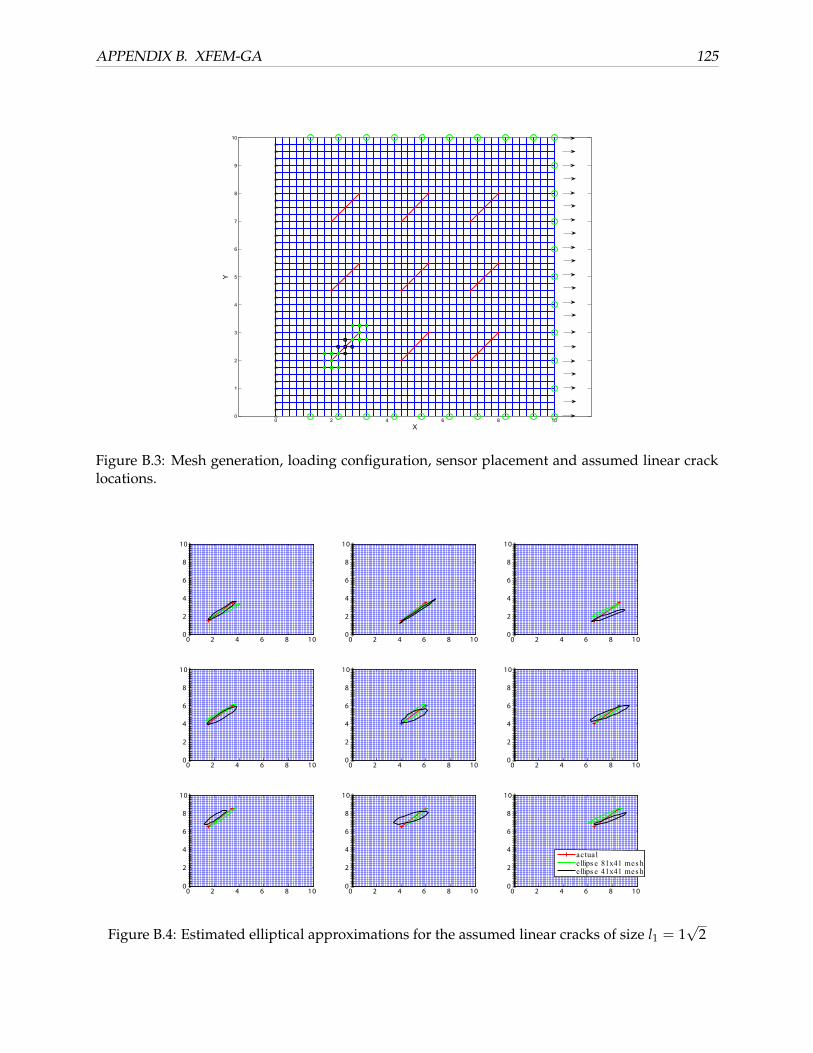
APPENDIX B. XFEM-GA 125
0 2 4 6 8 100
1
2
3
4
5
6
7
8
9
10
X
Y
Figure B.3: Mesh generation, loading configuration, sensor placement and assumed linear cracklocations.
0 2 4 6 8 100
2
4
6
8
10
0 2 4 6 8 100
2
4
6
8
10
0 2 4 6 8 100
2
4
6
8
10
0 2 4 6 8 100
2
4
6
8
10
0 2 4 6 8 100
2
4
6
8
10
0 2 4 6 8 100
2
4
6
8
10
0 2 4 6 8 100
2
4
6
8
10
0 2 4 6 8 100
2
4
6
8
10
0 2 4 6 8 100
2
4
6
8
10
actualellips e 81x41 mes hellips e 41x41 mes h
Figure B.4: Estimated elliptical approximations for the assumed linear cracks of size l1 = 1√
2

APPENDIX B. XFEM-GA 126
Table B.1: WAM-GA scheme
Mutation Pseudocodefor j=1,npop for k=1,nparam if (rand1 ≤ pc) /*perform mutation)*/ if (rand2 ≤ pwam) /*perform weighted average mutation)*/child(k, j)=child(k, j)+rand3 × (wmean(j)-child(k, j))else /*(perform standard creep mutation)*/child(k, j)=child(k, j)+g1(k) × crsgn
where,npop is the number of individuals per populationnparam is the number of parameters per candidate solution (individual)rand1,2,3 are random numbers uniformly distributed ∈ [0 1]pc is the creep mutation probabilityg1(k) is the incremental value between the upper and lower bound
for each parameter kcrsgn is equal to ±1 with a uniform probabilitypwam is the weighted average mutation probabilitychild(k, j) is the real value corresponding to parameter k of the j-th individual,andxm(k) is the weighted average for that parameter value by the end of the
previous generation obtained from:
xm(k) =∑i
wichild(k, i)
∑i
wi, wi =
1‖ f itness(i)‖+ ε
(B.5)
where, i is an index corresponding to each of the formed individuals up to that point of the evolu-tionary process, wi is the associated weight and ε is a sufficiently “small” numerical value addedfor the case where the fitness of the individual approaches 0. This particular expression has beenchosen for the type of problems considered herein aiming at minimizing a residual (error) func-tion toward zero. The formula yielding the weights can be properly modified for different classesof problems.

APPENDIX C. XICE 127
Appendix C
FEAP & Trilinos Implementations
In this chapter, the implementation details of the program XICE is presented.
C.1 FEAP User Element for 3D XFEM
A user element UEL is developed withing the finite element program FEAP to mode three dimen-
sional cracks. Listed below is a sample user input file and a description of using the XFEM user
elements. Here the solid elements to be checked are all assigned to MATErial 1 (XFEM elements).
A user mesh-manipulation command MANI is then called upon to identify the enriched elements
based on the nodal levelsets. This function automatically assigns all the non-enriched elements to
MATErial 2 which is the FEAP default solid elements.
The second line of the UEL input calls for the user element defined by ELMT01 (XFEM) to be
used. The third line of input requires four parameters to be defined. They are:
i. ncr: Number of crack planes
ii. gporder: Order of gauss quadrature for each tetrahedral subquadrature region for an en-
riched element
iii. tipon: A flag set to 0 or 1 to toggle tip enrichment on or off
iv. opflag: A flag set to 0 or 1 to toggle screen output from XFEM elements.
From the next line onwards, four sets of (x,y,z) points are specified and define the vertices of each
crack plane. For example, if ncr is 3, then 12 sets of points need to be specified.

APPENDIX C. XICE 128
Lastly the material properties to be used for the XFEM element are specified. Any standard
material definition that can be used in FEAP for solid continuum elements (small displacements)
can be specified. Please refer to the FEAP manual for details about this specification.
C.1.1 Input format
! MATERIAL 1 is XFEM user element
! -----------------------------------
MATErial 1
USER 1
1 11 0 0
x1 y1 z1
x1 y2 z2
x2 y2 z2
x2 y1 z1
SOLID
ELASTIC ISOTROPIC e nu
PLASTIC MISES ys
! MATERIAL 2 is regular solid element
! -----------------------------------
MATErial 2
SOLID
ELASTIC ISOTROPIC e nu
PLASTIC MISES ys
C.1.2 Stiffness generation for jump-enriched element
The code related to the generation of the element stiffness matrix for an XFEM element with jump-
entiched nodes is reproduced below.
subroutine XFEMnonlinstiff(d,ul,xl,tl,S,R,isw)
c SUBROUTINE TO COMPUTE THE STIFFNESS MATRIX OF A USER ELEMENT
use xfemvars
implicit none
include ’sdata.h’ !ndf,ndm,nen1,nst,nneq,ndl,nnlm,nadd
include ’eldata.h’ !dm,n,ma,mct,iel,nel,pstyp
include ’pointer.h’ !np,up
include ’comblk.h’ !hr(1),mr(1)
include ’cdata.h’ !numnp,numel,nummat,nen,neq,ipr
include ’hdata.h’ !nh1,nh2,nh3,ht1,ht2,ht3
include ’iofile.h’
include ’bdata.h’
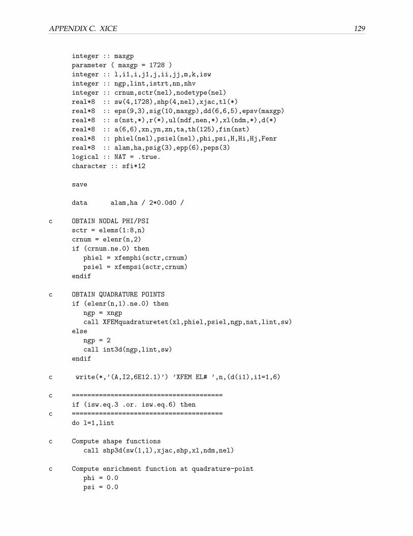
APPENDIX C. XICE 129
integer :: maxgp
parameter ( maxgp = 1728 )
integer :: l,i1,i,j1,j,ii,jj,m,k,isw
integer :: ngp,lint,istrt,nn,nhv
integer :: crnum,sctr(nel),nodetype(nel)
real*8 :: sw(4,1728),shp(4,nel),xjac,tl(*)
real*8 :: eps(9,3),sig(10,maxgp),dd(6,6,5),epsv(maxgp)
real*8 :: s(nst,*),r(*),ul(ndf,nen,*),xl(ndm,*),d(*)
real*8 :: a(6,6),xn,yn,zn,ta,th(125),fin(nst)
real*8 :: phiel(nel),psiel(nel),phi,psi,H,Hi,Hj,Fenr
real*8 :: alam,ha,psig(3),epp(6),peps(3)
logical :: NAT = .true.
character :: sfi*12
save
data alam,ha / 2*0.0d0 /
c OBTAIN NODAL PHI/PSI
sctr = elems(1:8,n)
crnum = elenr(n,2)
if (crnum.ne.0) then
phiel = xfemphi(sctr,crnum)
psiel = xfempsi(sctr,crnum)
endif
c OBTAIN QUADRATURE POINTS
if (elenr(n,1).ne.0) then
ngp = xngp
call XFEMquadraturetet(xl,phiel,psiel,ngp,nat,lint,sw)
else
ngp = 2
call int3d(ngp,lint,sw)
endif
c write(*,’(A,I2,6E12.1)’) ’XFEM EL# ’,n,(d(i1),i1=1,6)
c =======================================
if (isw.eq.3 .or. isw.eq.6) then
c =======================================
do l=1,lint
c Compute shape functions
call shp3d(sw(1,l),xjac,shp,xl,ndm,nel)
c Compute enrichment function at quadrature-point
phi = 0.0
psi = 0.0

APPENDIX C. XICE 130
do i = 1,nel
phi = phi + shp(4,i)*phiel(i)
psi = psi + shp(4,i)*psiel(i)
nodetype(i) = ndenr(sctr(i),1)
enddo
call Heaviside(H,phi)
c Compute strain at point
call XFEMstrn3d(d,xl,ul,th,shp,eps,ta,H,phiel)
c Compute stress at point
call modlsd(d,ta,eps,hr(nh1+nn),hr(nh2+nn),nhv,istrt,
& dd,sig(1,l),alam,ha,isw)
c Compute d * b matrix = adb
i1 = 1
do i = 1,nel
xn = shp(1,i)*xjac*sw(4,l)
yn = shp(2,i)*xjac*sw(4,l)
zn = shp(3,i)*xjac*sw(4,l)
call Heaviside(Hi,xfemphi(sctr(i),crnum))
a(1,1) = xn*dd(1,1,1) + yn*dd(4,1,1) + zn*dd(6,1,1)
a(1,2) = xn*dd(1,2,1) + yn*dd(4,2,1) + zn*dd(6,2,1)
a(1,3) = xn*dd(1,3,1) + yn*dd(4,3,1) + zn*dd(6,3,1)
a(1,4) = xn*dd(1,4,1) + yn*dd(4,4,1) + zn*dd(6,4,1)
a(1,5) = xn*dd(1,5,1) + yn*dd(4,5,1) + zn*dd(6,5,1)
a(1,6) = xn*dd(1,6,1) + yn*dd(4,6,1) + zn*dd(6,6,1)
a(2,1) = xn*dd(4,1,1) + yn*dd(2,1,1) + zn*dd(5,1,1)
a(2,2) = xn*dd(4,2,1) + yn*dd(2,2,1) + zn*dd(5,2,1)
a(2,3) = xn*dd(4,3,1) + yn*dd(2,3,1) + zn*dd(5,3,1)
a(2,4) = xn*dd(4,4,1) + yn*dd(2,4,1) + zn*dd(5,4,1)
a(2,5) = xn*dd(4,5,1) + yn*dd(2,5,1) + zn*dd(5,5,1)
a(2,6) = xn*dd(4,6,1) + yn*dd(2,6,1) + zn*dd(5,6,1)
a(3,1) = xn*dd(6,1,1) + yn*dd(5,1,1) + zn*dd(3,1,1)
a(3,2) = xn*dd(6,2,1) + yn*dd(5,2,1) + zn*dd(3,2,1)
a(3,3) = xn*dd(6,3,1) + yn*dd(5,3,1) + zn*dd(3,3,1)
a(3,4) = xn*dd(6,4,1) + yn*dd(5,4,1) + zn*dd(3,4,1)
a(3,5) = xn*dd(6,5,1) + yn*dd(5,5,1) + zn*dd(3,5,1)
a(3,6) = xn*dd(6,6,1) + yn*dd(5,6,1) + zn*dd(3,6,1)
! Heaviside-enriched-nodes a(4:6,1:6) = a(1:3,1:6)*Fenr
Fenr = dabs(H-Hi)
if (nodetype(i).eq.1) then

APPENDIX C. XICE 131
do ii = 1,3
do jj = 1,6
a(ii + 3,jj) = a(ii,jj)*Fenr
enddo
enddo
endif
c Compute stiffness matrix
j1 = 1
do j = 1,nel
xn = shp(1,j)
yn = shp(2,j)
zn = shp(3,j)
s(i1 ,j1 ) = s(i1 ,j1 ) + a(1,1)*xn + a(1,4)*yn + a(1,6)*zn
s(i1 ,j1+1) = s(i1 ,j1+1) + a(1,4)*xn + a(1,2)*yn + a(1,5)*zn
s(i1 ,j1+2) = s(i1 ,j1+2) + a(1,6)*xn + a(1,5)*yn + a(1,3)*zn
s(i1+1,j1 ) = s(i1+1,j1 ) + a(2,1)*xn + a(2,4)*yn + a(2,6)*zn
s(i1+1,j1+1) = s(i1+1,j1+1) + a(2,4)*xn + a(2,2)*yn + a(2,5)*zn
s(i1+1,j1+2) = s(i1+1,j1+2) + a(2,6)*xn + a(2,5)*yn + a(2,3)*zn
s(i1+2,j1 ) = s(i1+2,j1 ) + a(3,1)*xn + a(3,4)*yn + a(3,6)*zn
s(i1+2,j1+1) = s(i1+2,j1+1) + a(3,4)*xn + a(3,2)*yn + a(3,5)*zn
s(i1+2,j1+2) = s(i1+2,j1+2) + a(3,6)*xn + a(3,5)*yn + a(3,3)*zn
if (nodetype(j).eq.1) then
! bottom left
do m = 4,6
k = m - 1
s(i1+k,j1 ) = s(i1+k,j1 ) + a(m,1)*xn + a(m,4)*yn + a(m,6)*zn
s(i1+k,j1+1) = s(i1+k,j1+1) + a(m,4)*xn + a(m,2)*yn + a(m,5)*zn
s(i1+k,j1+2) = s(i1+k,j1+2) + a(m,6)*xn + a(m,5)*yn + a(m,3)*zn
enddo
! dNd(X,Y,Z) * (H-Hj)
call Heaviside(Hj,xfemphi(sctr(j),crnum))
Fenr = dabs(H-Hj)
xn = xn*Fenr
yn = yn*Fenr
zn = zn*Fenr
do m = 1,6
! Top/bottom-right
k = m-1
s(i1+k,j1+3) = s(i1+k,j1+3) + a(m,1)*xn + a(m,4)*yn + a(m,6)*zn

APPENDIX C. XICE 132
s(i1+k,j1+4) = s(i1+k,j1+4) + a(m,4)*xn + a(m,2)*yn + a(m,5)*zn
s(i1+k,j1+5) = s(i1+k,j1+5) + a(m,6)*xn + a(m,5)*yn + a(m,3)*zn
enddo
endif
j1 = j1 + ndf
end do ! j
i1 = i1 + ndf
end do ! i
enddo ! Quadrature points
do i = 1,nst
fin(i) = r(i)
enddo
call XFEMresid3d(s,ul,fin,r,nst)
c ===========================================
elseif (isw.eq.4 .or. isw.eq.8 .or. isw.eq.16) then
c ===========================================
nn = 0
do l = 1,lint
c Compute shape functions
call shp3d(sw(1,l),xjac,shp,xl,ndm,nel)
c Compute enrichment function at quadrature-point
phi = 0.0
psi = 0.0
do i = 1,nel
phi = phi + shp(4,i)*phiel(i)
psi = psi + shp(4,i)*psiel(i)
nodetype(i) = ndenr(sctr(i),1)
enddo
call Heaviside(H,phi)
c Compute strain at point
call XFEMstrn3d(d,xl,ul,th,shp,eps,ta,H,phiel)
c Compute stress at point
call modlsd(d,ta,eps,hr(nh1+nn),hr(nh2+nn),nhv,istrt,
& dd,sig(1,l),alam,ha,isw)
C Output values
if(isw.eq.4) then
c Compute coordinates

APPENDIX C. XICE 133
xn = 0.0
yn = 0.0
zn = 0.0
do j = 1,nel
xn = xn + shp(4,j)*xl(1,j)
yn = yn + shp(4,j)*xl(2,j)
zn = zn + shp(4,j)*xl(3,j)
end do ! j
c Compute principal stress values
do i = 1,3
epp(i ) = eps(i ,1)
epp(i+3) = eps(i+3,1)*0.5d0
end do ! i
call pstr3d(sig(1,l),psig)
call pstr3d(epp ,peps)
mct = mct - 5
if(mct.le.0) then
write(iow,2010) o,head
if(ior.lt.0) write(*,2010) o,head
mct = 50
endif
write(iow,2011) n,ma,xn,yn,zn,
& (sig(i,l),i=1,6),(epp(i),i=1,6),
& (psig(i),i=1,3),(peps(i),i=1,3)
if(ior.lt.0) then
write(*,2011) n,ma,xn,yn,zn,
& (sig(i,l),i=1,6),(epp(i),i=1,6),
& (psig(i),i=1,3),(peps(i),i=1,3)
endif
endif
nn = nn + nhv
end do ! l
c Plot stress values
if(isw.eq.8) then
call slcn3d(sig, r,s, nel)
c Compute J-integrals and material forces
elseif(isw.eq.16) then
call pjint3d(ul,tl,epsv,sig,r,ndf,ndm)
endif
endif

APPENDIX C. XICE 134
c Formats
2010 format(a1,20a4//5x,’Element Stresses’//’ Elmt Mat’,
& ’ 1-coord 2-coord 3-coord’/12x,
& ’ 11-stress 22-stress 33-stress 12-stress’,
& ’ 23-stress 31-stress’/12x,
& ’ 11-strain 22-strain 33-strain 12-strain’,
& ’ 23-strain 31-strain’/12x,
& ’ 1-stress 2-stress 3-stress’,
& ’ 1-strain 2-strain 3-strain’,/39(’ -’))
2011 format(/i9,i4,1p,3e11.3/(12x,1p,6e11.3))
end subroutine XFEMnonlinstiff