Embed Size (px)
Citation preview

The Dissertation Committee for Sara Navidi certifies that this is the approved version of the following dissertation:
Development of Site Amplification Model for Use in
Ground Motion Prediction Equations
Committee: ____________________________________ Ellen M. Rathje, Supervisor ____________________________________ Robert B. Gilbert ____________________________________ Chadi El Mohtar ____________________________________ Lance Manuel ____________________________________ Thomas W. Sager

Development of Site Amplification Model for Use in
Ground Motion Prediction Equations
by
Sara Navidi, B.S.; M.S.
Dissertation
Presented to the Faculty of the Graduate School of
The University of Texas at Austin
in Partial Fulfillment
of the Requirements
for the Degree of
Doctor of Philosophy
The University of Texas at Austin
May 2012

To my parents

iv
Development of Site Amplification Model for Use in
Ground Motion Prediction Equations
Sara Navidi, Ph.D.
The University of Texas at Austin, 2012
Supervisor: Ellen M. Rathje
The characteristics of earthquake shaking are affected by the local site conditions.
The effects of the local soil conditions are often quantified via an amplification factor
(AF), which is defined as the ratio of the ground motion at the soil surface to the
ground motion at a rock site at the same location. Amplification factors can be
defined for any ground motion parameter, but most commonly are assessed for
acceleration response spectral values at different oscillator periods. Site
amplification can be evaluated for a site by conducting seismic site response
analysis, which models the wave propagation from the base rock through the site-
specific soil layers to the ground surface. An alternative to site-specific seismic
response analysis is site amplification models. Site amplification models are
empirical equations that predict the site amplification based on general
characteristics of the site. Most of the site amplification models that already used in
v
ground motion prediction equations characterize a site with two parameters: the
average shear wave velocity in the top 30 m (VS30) and the depth to bedrock.
However, additional site parameters influence site amplification and should be
included in site amplification models.
To identify the site parameters that help explain the variation in site
amplification, ninety nine manually generated velocity profiles are analyzed using
seismic site response analysis. The generated profiles have the same VS30 and depth
to bedrock but a different velocity structure in the top 30 m. Different site
parameters are investigated to explain the variability in the computed amplification.
The parameter Vratio, which is the ratio of the average shear wave velocity between
20 m and 30 m to the average shear wave velocity in the top 10 m, is identified as
the site parameter that most affects the computed amplification for sites with the
same VS30 and depth to bedrock.
To generalize the findings from the analyses in which only the top 30 m of the
velocity profile are varied, a suite of fully randomized velocity profiles are generated
and site response analysis is used to compute the amplification for each site for a
range of input motion intensities. The results of the site response analyses
conducted on these four hundred fully randomized velocity profiles confirm the
influence of Vratio on site amplification. The computed amplification factors are
used to develop an empirical site amplification model that incorporates the effect of
Vratio, as well as VS30 and the depth to bedrock. The empirical site amplification

vi
model includes the effects of soil nonlinearity, such that the predicted amplification
is a function of the intensity of shaking. The developed model can be incorporated
into the development of future ground motion prediction equations.

vii
Contents
Development of Site Amplification Model for Use in Ground Motion Prediction
Equations .................................................................................................................................................. iv
Chapter 1 Introduction ........................................................................................................................ 1
1.1Research Significance ................................................................................................................. 1
1.2 Research Objectives ................................................................................................................... 4
1.3 Outline of Dissertation .............................................................................................................. 5
Chapter 2 Modeling Site Amplification in Ground Motion Prediction Equations ........ 6
2.1 Introduction .................................................................................................................................. 6
2.2 Site Amplification Models ........................................................................................................ 7
2.2.1 VS30 Scaling ...................................................................................................................... 8
2.2.2 Soil Depth Scaling ......................................................................................................... 19
2.3 Unresolved Issues .................................................................................................................... 24
Chapter 3 Identification of Site Parameters that Influence Site Amplification ............ 26
3.1 Introduction................................................................................................................................ 26
3.2 Site Profiles ................................................................................................................................. 27
3.3 Input Motions ............................................................................................................................ 32
3.4 Site Characteristics .................................................................................................................. 34
3.5 Amplification at Low Input Intensities ............................................................................ 39
3.5.1 Variability in Amplification Factors .............................................................................. 39
3.5.2 Identification of site parameters that explain variation in AF...................................... 43
3.6 Amplification at Moderate Input Intensities ................................................................. 53
viii
3.6.1 Variability in Amplification Factors .............................................................................. 53
3.6.2 Influence of site parameters on site amplification ...................................................... 57
3.7 Amplification at High Input Intensities ........................................................................... 63
3.7.1 Variability in Amplification Factors .............................................................................. 63
3.7.2 Influence of site parameters on site amplification ...................................................... 66
3.8 Summary...................................................................................................................................... 70
Chapter 4 Statistical Generation of Velocity Profiles ............................................................. 72
4.1 Introduction................................................................................................................................ 72
4.2 Development of Randomized Velocity Profiles for Site Response Analysis ...... 73
4.2.1 Modeling Variations in Site Properties ......................................................................... 73
4.2.2 Baseline Profiles ........................................................................................................... 78
4.2.3 Generated Shear Wave Velocity Profiles ..................................................................... 83
4.3 Approach to Development of Amplification Model ..................................................... 88
4.4 Summary...................................................................................................................................... 93
Chapter 5 Models for Linear Site Amplification ....................................................................... 94
5.1 Introduction................................................................................................................................ 94
5.2 Linear Site Amplification (PGArock=0.01g)...................................................................... 94
5.3 Influence of Vratio on Amplification ............................................................................... 105
5.4 Influence of Z1.0 on Amplification for Long Periods .................................................. 119
5.5 Summary.................................................................................................................................... 128
Chapter 6 Models for Nonlinear Site Amplification .............................................................. 129
6.1 Introduction ............................................................................................................................. 129
6.2 VS30 Scaling for Nonlinear Models .................................................................................... 130
6.3 Nonlinear Site Amplification at Short Periods ............................................................ 133
6.3.1 Influence of Vratio on Nonlinear Site Response......................................................... 139
6.4 Nonlinear Site Amplification at Long Periods ............................................................. 148
6.5 Summary.................................................................................................................................... 154
Chapter 7 Final Site Amplification Model ................................................................................. 155
7.1 Introduction ............................................................................................................................. 155

ix
7.2 Combined Model for Short Periods ................................................................................. 156
7.3 Combined Model for Long Periods .................................................................................. 170
7.4 Summary.................................................................................................................................... 179
Chapter 8 Amplification Prediction ............................................................................................ 180
8.1 Introduction ............................................................................................................................. 180
8.2 Scenario Events ....................................................................................................................... 180
8.3 Site Amplification Predicted by NGA Models .............................................................. 182
8.4 Site Amplification Predicted by the Developed Model ............................................ 185
8.4 Limitations of the Proposed Model ................................................................................. 190
8.5 Summary.................................................................................................................................... 193
Chapter 9 Summary, Conclusions, and Recommendations ............................................... 194
9.1 Summary and Conclusions ................................................................................................. 194
9.2 Recommendations for Future Work ............................................................................... 197
Bibliography......................................................................................................................................... 199

1
Chapter 1
Introduction
1.1 Research Significance
When an earthquake occurs, seismic waves are released at the source (fault), they
travel through the earth, and they generate ground shaking at the ground surface.
The characteristics of shaking at a site depend on the source characteristics and
change as they travel through their path to get to the site (Figure 1.1). The wave
amplitudes generally attenuate with distance as they travel through the bedrock in
the crust (i.e. path effect) and they are modified by the local soil conditions at the
site (i.e. site effect). The important property of the local soil conditions that
influence ground shaking is the shear wave velocity. Although seismic waves may
travel a longer distance through the bedrock than through the local soils, the
influence of the local soil conditions can be significant.

2
Figure 1.1 Propagation of seismic waves from source to surface.PSL, http://seismo.geology.upatras.gr/MICROZON-THEORY1.htm
The effects of the local soil conditions are often quantified via an amplification
factor (AF), which is defined as the ratio of the ground motion at the soil surface to
the ground motion at a rock site at the same location. Amplification factors can be
defined for any ground motion parameter, but most commonly are assessed for
acceleration response spectral values at different periods.
Two main alternatives are available to evaluate the amplification of acceleration
response spectra due to local soil conditions:
o Site-specific Site Response Analysis
o Empirical Ground Motion Prediction Equations

3
Site response analysis propagates waves from the underlying bedrock through the
soil layers to the ground surface. Most often site response analysis is performed
using a one-dimensional assumption in which the soil and bedrock surfaces extend
infinitely in the horizontal direction and all boundaries are assumed horizontal. The
nonlinear response of the soil can be modeled via the equivalent linear
approximation or through fully nonlinear approaches. Site response analysis
provides a detailed assessment of site amplification but requires significant
information about the site, including the shear wave velocity profile from the
surface down to bedrock and characterization of nonlinear soil properties, as well as
selection of appropriate input rock motions.
An alternative to site-specific site response analysis is an empirical estimate of
site amplification that uses an empirical equation to predict the site amplification
based on the input motion and the general characteristics of the site. This approach
is incorporated in empirical ground motion prediction equations (GMPEs). GMPEs
are statistical models that predict an acceleration response spectrum at a site as a
function of earthquake magnitude (M), site to source distance (R), local site
conditions, and other parameters. GMPEs are developed predominantly from
recorded ground motions from previous earthquakes. To account for local site
conditions, the site is characterized simply by one or two parameters (e.g. the
average shear wave velocity over the top 30 m) and the amplification at each period
is related to these parameters. The amplification relationship included in a ground
4
motion prediction equation is often called a site response or site amplification
model. While these models are relatively simple, and ignore important details about
the shear wave velocity profile and nonlinear properties at a site, they are important
tools that can be used to estimate site amplification for a range of applications. Yet
enhancements in these models can be made to improve their ability to predict site
amplification.
1.2 Research Objectives
The main objective of this research is to improve the site amplification models
included in ground motion prediction equations. Important site details that control
site amplification will be identified and statistical models will be developed that
include these parameters. These models then can be implemented in ground motion
prediction equations. To meet these objectives, first the important site parameters
that influence site amplification are identified. To identify these site parameters,
hypothetical shear wave velocity profiles are generated and their seismic response
computed using the equivalent linear approach. Various site parameters are
computed from the hypothetical velocity profiles and the relationship between each
of these parameters and the computed site amplification. After identifying
appropriate site parameters for use in the empirical site amplification model,
appropriate functional forms for the statistical model are developed. The developed
functional forms are fit to the computed amplification data.
5
1.3 Outline of Dissertation
The following dissertation consists of nine chapters. After the Introduction in
Chapter 1, Chapter 2 introduces modeling site amplification in ground motion
prediction equations and reviews the current state-of-the-art in site amplification
models. Identification of site parameters that affect site amplification is discussed in
Chapter 3. In this chapter sites with manually generated shear wave velocity profiles
are used to identify the parameters that most strongly influence the computed site
amplification. Chapter 4 presents the statistical generation of fully randomized
shear wave velocity profiles that are used to compute amplification factors for use in
developing the site amplification model. The nonlinear soil properties and the input
motions that are applied to these sites are also discussed in this chapter. In Chapter
5 through 7, the process of developing the functional form of the site amplification
model that includes the identified site parameters is presented. Chapter 5 discusses
the component of the proposed model for linear-elastic conditions and the
nonlinear component is discussed in Chapter 6. In Chapter 7, the linear and
nonlinear components of the developed functional form are combined and the final
model is presented. Chapter 8 demonstrates how the proposed model works to
predict the surface response spectrum of an actual site, and also compares the
developed amplification model with models developed by other researchers.
Chapter 9 provides a summary, conclusions, and recommendations for future
studies.
6
Chapter 2
Modeling Site Amplification in Ground
Motion Prediction Equations
2.1 Introduction
Site amplification has been included in ground motion prediction equations (GMPE)
for several decades. The initial site amplification models simply distinguished
between rock and soil sites and incorporated the site amplification by a scaling
parameter or by defining different statistical models for soil and rock sites (e.g.
Boore et al 1993; Campbell 1993; and Sadigh et al 1997). The ground motion
prediction equation of Abrahamson and Silva (1997) was the first to include
nonlinear effects in the site amplification model. Nonlinear effects represent the
influence of soil nonlinearity, where the stiffness of the soil decreases and the
damping increases as larger shear strains are induced in the soil. As a result of soil
nonlinearity, amplification is a nonlinear function of the input rock motion. While
the incorporation of nonlinear effect in the Abrahamson and Silva (1997) GMPE was

7
an improvement, the model only distinguishes between soil and rock, and did not
directly use shear wave velocity information in the amplification prediction. Boore
et al (1997) was the first to directly use the average shear wave velocity in the top
30 m (VS30) to predict site amplification, but their model did not include soil
nonlinearity.
The evolution of site amplification models used in GMPEs is described in the
next sections.
2.2 Site Amplification Models
The general form of a ground motion prediction equation is:
ln(Sa) = fm + fR + fsite (2.1)
where Sa is the spectral acceleration at a given period and fm , fR, and fsite are
functions that represent the ground motion scaling that accounts for magnitude (fm),
site-to-source distance (fR ), and site effects (fsite). The function fsite is considered the
“Site Amplification Model” or “Site Response Model” in the ground motion
prediction equation and it includes parameters that describe the site and the rock
input motion intensity.
An alternative form of equation (2.1) can be written in terms of the spectral
acceleration on soil (Sasoil), the spectral acceleration on rock (Sarock), and an
amplification factor (AF) using:
8
Sasoil = Sarock AF (2.2)
ln(Sasoil) = ln(Sarock AF) = ln(Sarock) + ln(AF) (2.3)
Comparing equations (2.1) and (2.3), it is clear that fm and fR work together to predict
ln (Sarock) and fsite represents ln(AF).
Researchers have modeled ln(AF) using different parameters and functional
forms, but most models incorporate the effects of VS30 (i.e., VS30 scaling). Some
models incorporate the effects of the soil depth (i.e., soil depth scaling).
2.2.1 VS30 Scaling
VS30 is computed from the travel time for a shear wave travelling through the top 30
m of a site. It is computed by:
S m
S i
ni
(2.4)
where VS,i is the shear wave velocity of layer i, and hi is the thickness of layer i. Only
layers within the top 30 m are used in this calculation.
The scaling of ground motions with respect to VS30 generally consists of two
terms: a linear-elastic term that is a function of VS30 alone, and a nonlinear term that
accounts for nonlinear soil effects. The nonlinear term is a function of both VS30 and
9
the input rock intensity. The linear term represents site amplification at small input
intensities where the soil response is essentially linear elastic. The nonlinear term
incorporates the effect of soil nonlinearity at larger input intensities. The resulting
functional form for the site amplification model (ln(AF)) is:
ln(AF) = fsite = ln(AF)LN + ln(AF)NL (2.5)
Boore et al (1997) were the first to use VS30 in their site amplification model.
Their model did not include nonlinearity effect and is written as:
(2.6)
where a and Vref are coefficients estimated by regression. In their model
amplification varies log-linearly with VS30.
Choi and Stewart (2005) expanded the Boore et al. (1997) site amplification
model to include both linear and nonlinear site amplification effects. The general
form of the model is given as:
(2.7)
where PGArock is the peak ground acceleration on rock in g unit, 0.1 is the reference
PGArock level for nonlinear behavior, and b is a function of VS30. This model does not
explicitly separate the linear and nonlinear components, because the
term contributes to the AF prediction at small values of PGArock.

10
The Choi and Stewart (2005) model was developed by considering recorded
ground motions at sites with known VS30 and computing the difference between the
observed ln(Sa) and the ln(Sa) predicted by an empirical ground motion prediction
equation for rock conditions. This difference represents ln(AF) because the
observed motion is ln(Sa,soil) and the predicted motion on rock is ln(Sa,rock).
Using the observed ln(AF), Choi and Stewart (2005) found that b is negative and
generally decreases towards zero as VS30 increases (Figure 2.1). This decrease in b
with increasing VS30 indicates that nonlinearity becomes less significant as sites
become stiffer.
Figure 2.2 shows predictions of amplification versus PGArock for three sites with
VS30= 250 m/s, 350 m/s, and 550 m/s using the Choi and Stewart (2005) model.
Amplification is shown for PGA and a spectral period of 0.2 s. For all three shown
sites, amplification decreases as input intensity increases. The softest site (i.e.,
VS30=250 m/s) has the greatest reduction in amplification. Again, note that the
nonlinear component of the Choi and Stewart (2005) model extends to small
PGArock, as the AF continues to change as PGA decreases to small values.

11
Figure 2.1 Derived values of b as a function of VS30 by Choi and Stewart (2005) for periods of 0.3 and 1.0 s.
Figure 2.2 Amplification for PGA and T=0.2 s as a function of input intensity (PGArock) as predicted by Choi and Stewart (2005) for a range of VS30.

12
Walling et al (2008) proposed a more complex site response model including the
nonlinear effect:
(2.8)
where the linear component of the model is similar those previously discussed (with
Vlin similar to Vref), but the nonlinear component is different. The main difference
between the Walling et al. (2008) model and the approach of Choi and Stewart
(2005) is the treatment of the coefficient b. Walling et al. (2008) models b as
independent of VS30 and adds a parameter to the input intensity that is VS30-
dependent (i.e.,
). With derived values of c and n positive, the functional
form in equation (2.8) results in the term
decreasing with decreasing
VS30. This results in soil nonlinearity affecting smaller VS30 more than larger VS30.
Walling et al. (2008) developed the regression parameters for equation (2.8)
using simulated amplification factors computed using the equivalent-linear method.
Figure 2.3 shows the predicted amplification versus input intensity for two sites
with VS30= 270 and 560m/s at spectral period of 0.2s as presented in Walling et al.
(2008). Amplification decreases when the input intensity increases and the
reduction in amplification with input intensity is larger for the softer site (i.e.,
VS30=270 m/s). The Walling et al (2008) model was developed using simulations of
sites with VS30 between 270 m/s and 900 m/s.

13
Figure 2.3 Example of the parametric fit for VS30=270 and 560 m/s using equation (2.8) at T=0.2 s (Walling et al 2008).
The current state–of-the-art in GMPEs is represented by models developed in
the “Next Generation of Ground-Motion Attenuation Models” (NGA) project
(peer.berkeley.edu/ngawest). This effort took place over five years to develop
improved GMPEs for shallow crustal earthquake in the western U.S. and similar
active tectonic zones. This effort was organized by the Pacific Earthquake
Engineering Research center (PEER). Different GMPE were developed by five teams:
Abrahamson and Silva (2008), Boore and Atkinson (2008), Campbell and Bozorgnia
(2008), Chiou and Youngs (2008), and Idriss (2008). Although each team developed
their own GMPE, the teams interacted with one another extensively. They all used
the same database of recorded ground motions, but they were free to use the entire
database or select subsets of it. The site amplification models included in the NGA

14
relationships are discussed below. The Idriss (2008) model is not discussed
because it does not explicitly use VS30.
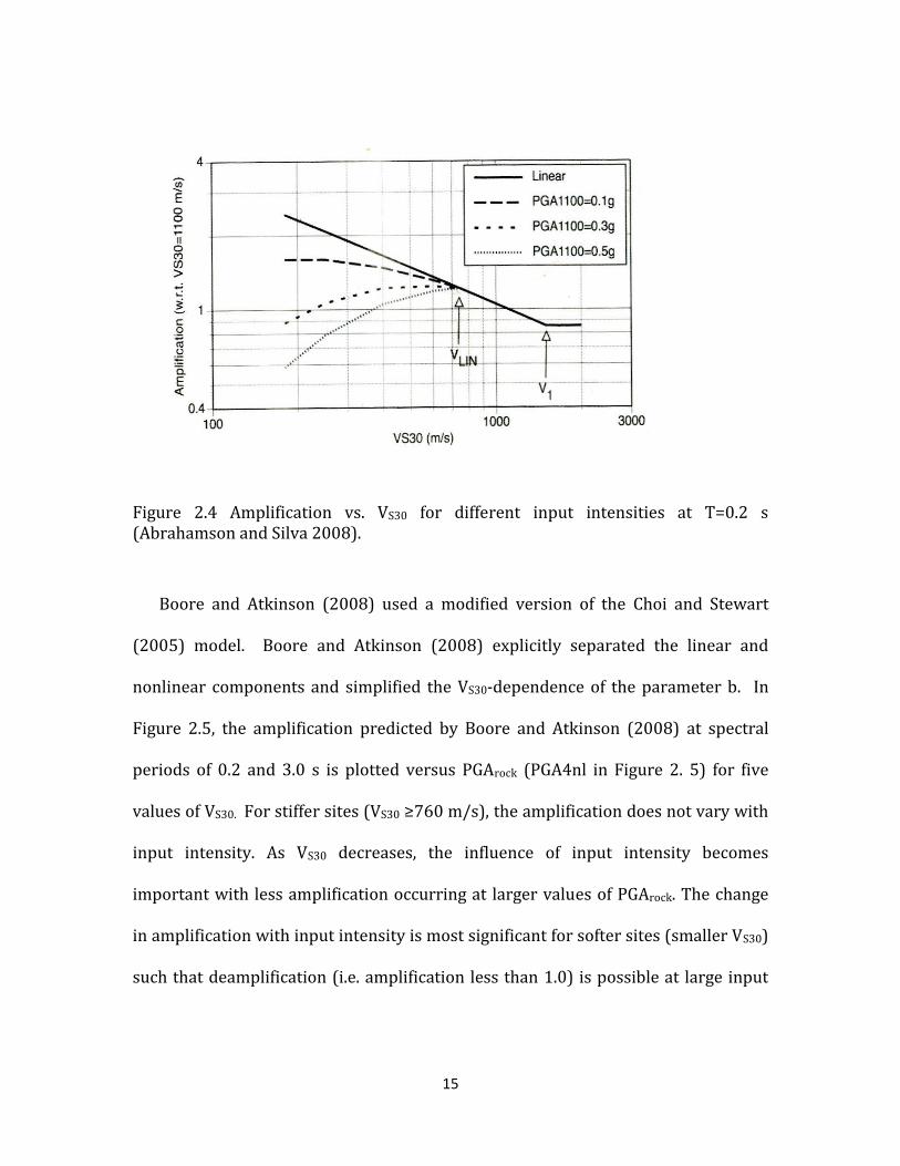
Abrahamson and Silva (2008) adopted the form of the nonlinear site
amplification model developed by Walling et al (2008). The regression coefficients
for the nonlinear component of the site amplification model were constrained by the
values obtained by Walling et al. (2008). Only the coefficient for the linear-elastic
component of the model (i.e., a) term was estimated in the regression analysis from
the recorded motions. Figure 2.4 shows the variation of amplification with VS30
under four different shaking levels using the Abrahamson and Silva (2008) site
amplification model for T=0.2 s. The amplification model shows that the
amplification decreases with increasing PGArock for VS30 smaller than Vlin. The
reduction in AF with increasing PGArock is strongest at the smallest VS30.
15
Figure 2.4 Amplification vs. VS30 for different input intensities at T=0.2 s (Abrahamson and Silva 2008).
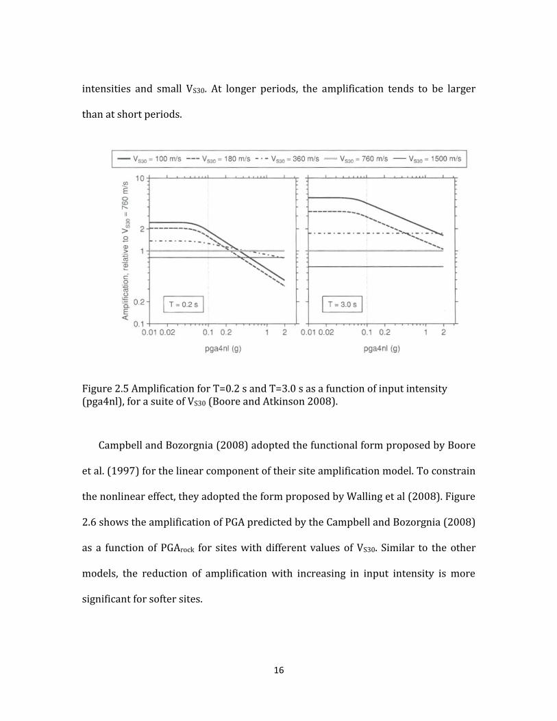
Boore and Atkinson (2008) used a modified version of the Choi and Stewart
(2005) model. Boore and Atkinson (2008) explicitly separated the linear and
nonlinear components and simplified the VS30-dependence of the parameter b. In
Figure 2.5, the amplification predicted by Boore and Atkinson (2008) at spectral
periods of 0.2 and 3.0 s is plotted versus PGArock (PGA4nl in Figure 2. 5) for five
values of VS30. For stiffer sites (VS30 ≥760 m/s), the amplification does not vary with
input intensity. As VS30 decreases, the influence of input intensity becomes
important with less amplification occurring at larger values of PGArock. The change
in amplification with input intensity is most significant for softer sites (smaller VS30)
such that deamplification (i.e. amplification less than 1.0) is possible at large input
16
intensities and small VS30. At longer periods, the amplification tends to be larger
than at short periods.
Figure 2.5 Amplification for T=0.2 s and T=3.0 s as a function of input intensity (pga4nl), for a suite of VS30 (Boore and Atkinson 2008).
Campbell and Bozorgnia (2008) adopted the functional form proposed by Boore
et al. (1997) for the linear component of their site amplification model. To constrain
the nonlinear effect, they adopted the form proposed by Walling et al (2008). Figure
2.6 shows the amplification of PGA predicted by the Campbell and Bozorgnia (2008)
as a function of PGArock for sites with different values of VS30. Similar to the other
models, the reduction of amplification with increasing in input intensity is more
significant for softer sites.

17
Figure 2.6 Amplification for PGA as a function of input intensity (PGA on rock), for a suite of VS30 (Campbell and Bozorgnia 2008).
Chiou and Youngs (2008) used a modified version of Choi and Stewart (2005)
site amplification model. While Choi and Stewart (2005) normalized PGArock by 0.1
g, Chiou and Youngs (2008) use the following form:
(2.9)
This functional form separates the linear and nonlinear components because for
small Sarock, the
term will tend to zero. Chiou and Youngs (2008) model
b as VS30-dependent.

18
Figure 2.7 plots amplification versus VS30 for different input intensities as
predicted by the Chiou and Youngs (2008) NGA model. Amplification is shown for
spectral periods of 0.01, 0.1, 0.3, and 1.0 sec. At small input intensities (i.e. 0.01g)
where the linear term dominates, amplification increases log-linearly as VS30
decreases. This effect is larger at longer periods. At larger input intensities, the
amplification at each VS30 is reduced due to soil nonlinearity (i.e. soil stiffness
reduction and increased damping). This effect is largest at small VS30 and shorter
periods.
Figure 2.7 Site amplification as a function of spectral period, VS30 and level of input intensity (Chiou and Youngs 2008).
19
2.2.2 Soil Depth Scaling
The Abrahamson and Silva (2008), Campbell and Bozorgnia (2008), and Chiou and
Youngs (2008) NGA models include a soil depth term in addition to VS30 when
predicting site amplification at long periods. Because the natural period of a soil site
is proportional to the soil depth (i.e., deeper sites have longer natural periods),
deeper soil sites will experience more amplification at long periods than shallow soil
sites. The scaling of site amplification with soil depth is commonly considered
independent of input intensity (i.e., not influenced by soil nonlinearity). Each NGA
model defines soil depth as the depth to a specific shear wave velocity horizon.
Abrahamson and Silva (2008) and Chiou and Youngs (2008) use the depth to VS
equal to or greater than 1.0 km/s (called Z1.0), while Campbell and Bozorgnia (2008)
use the depth to a VS equal to or greater than 2.5 km/s (called Z2.5). Essentially, Z1.0
represents the depth to “engineering” rock while Z2.5 represents the depth to hard
rock.
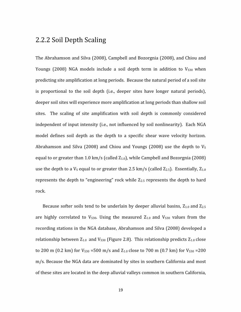
Because softer soils tend to be underlain by deeper alluvial basins, Z1.0 and Z2.5
are highly correlated to VS30. Using the measured Z1.0 and VS30 values from the
recording stations in the NGA database, Abrahamson and Silva (2008) developed a
relationship between Z1.0 and VS30 (Figure 2.8). This relationship predicts Z1.0 close
to 200 m (0.2 km) for VS30 =500 m/s and Z1.0 close to 700 m (0.7 km) for VS30 =200
m/s. Because the NGA data are dominated by sites in southern California and most
of these sites are located in the deep alluvial valleys common in southern California,

20
the depths are not necessarily representative of areas in other parts of the western
United States.
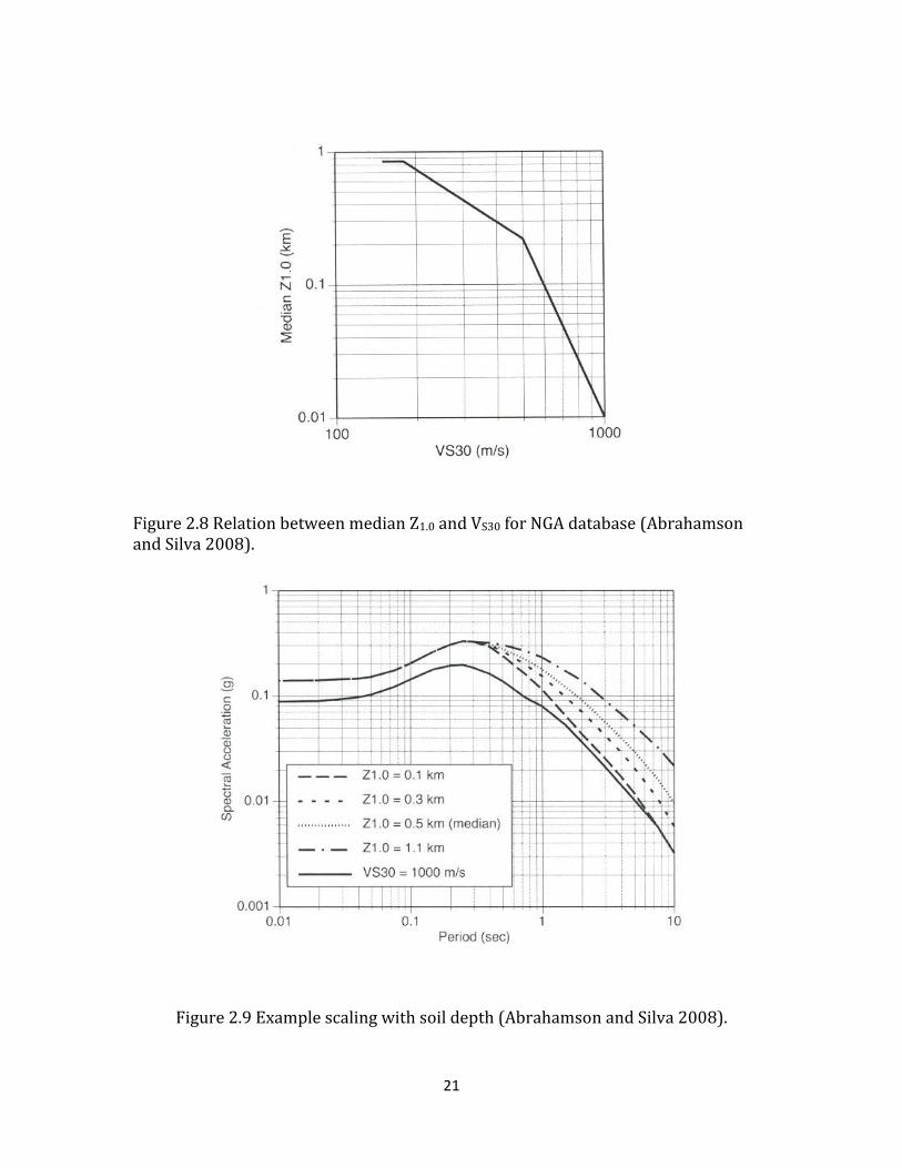
As noted previously, soil depth predominantly affects long period amplification
because soil depth affects the natural period of a site and the associated periods of
amplification. Figure 2.9 shows the predicted acceleration response spectra for a
soil site with VS30 = 270 m/s and different values of Z1.0 as predicted by the
Abrahamson and Silva (2008) NGA model for a M=7.0 earthquake at a distance of 30
km. At short periods (less than 0.4 s) Z1.0 does not influence the response spectrum,
while at longer periods the response spectra are significantly affected by Z1.0. For
example, at a spectral period of 1.0 s, the spectral acceleration for Z1.0=0.1 km is 0.08
while the spectral acceleration for Z1.0=1.1 km is close to 0.25. This represents an
amplification of greater than 3.0. At longer periods the effect of Z1.0 is even more
pronounced. At a spectral period of 5.0 s, the response spectra in Figure 2.9 indicate
an amplification of greater than 4.0 between Z1.0=0.1 km and 1.1 km.
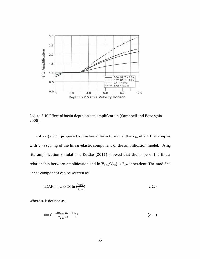
As mentioned previously, the Campbell and Bozorgnia (2008) model considers
the depth to the 2.5 km/s velocity horizon as the soil depth (Z2.5). Figure 2.10 shows
the site amplification as a function of Z2.5 as predicted by the Campbell and
Bozorgnia (2008) NGA model. The Z2.5 effect is only significant at deep sites (Z2.5> 3
km) with amplification as large as 2.0 to 3.0 for deep sites and long periods. There is
also a slight reduction in amplification for shallow profiles (Z2.5< 1.0 km).
21
Figure 2.8 Relation between median Z1.0 and VS30 for NGA database (Abrahamson and Silva 2008).
Figure 2.9 Example scaling with soil depth (Abrahamson and Silva 2008).
22
Figure 2.10 Effect of basin depth on site amplification (Campbell and Bozorgnia 2008).
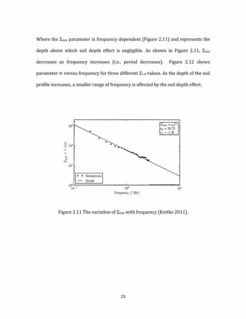
Kottke (2011) proposed a functional form to model the Z1.0 effect that couples
with VS30 scaling of the linear-elastic component of the amplification model. Using
site amplification simulations, Kottke (2011) showed that the slope of the linear
relationship between amplification and ln(VS30/Vref) is Z1.0 dependent. The modified
linear component can be written as:
(2.10)
Where is defined as:
(2.11)
23
Where the Zmin parameter is frequency dependent (Figure 2.11) and represents the
depth above which soil depth effect is negligible. As shown in Figure 2.11, Zmin
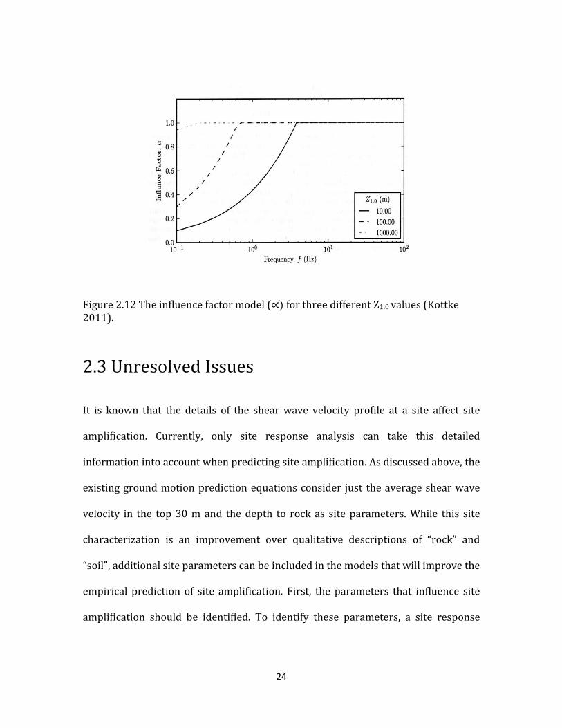
decreases as frequency increases (i.e., period decreases). Figure 2.12 shows
parameter versus frequency for three different Z1.0 values. As the depth of the soil
profile increases, a smaller range of frequency is affected by the soil depth effect.
Figure 2.11 The variation of Zmin with frequency (Kottke 2011).
24
Figure 2.12 The influence factor model ( for three different Z1.0 values (Kottke 2011).
2.3 Unresolved Issues
It is known that the details of the shear wave velocity profile at a site affect site
amplification. Currently, only site response analysis can take this detailed
information into account when predicting site amplification. As discussed above, the
existing ground motion prediction equations consider just the average shear wave
velocity in the top 30 m and the depth to rock as site parameters. While this site
characterization is an improvement over qualitative descriptions of “rock” and
“soil”, additional site parameters can be included in the models that will improve the
empirical prediction of site amplification. First, the parameters that influence site
amplification should be identified. To identify these parameters, a site response

25
study is performed as discussed in the next chapter. Then, the findings from these
analyses need to be expanded to any possible site. Numerous site profiles with a
wide range of site parameters should be analyzed. To be able to analyze a
reasonable number of soil profiles, 400 soil profiles are statistically generated and
analyzed. The response of the fully randomized profiles under different level of
input intensities are considered to develop a model that incorporates the effect of
the identified site parameters in site amplification.

26
Chapter 3
Identification of Site Parameters that
Influence Site Amplification
3.1 Introduction
As discussed in previous chapter, the average shear wave velocity in top 30 m (VS30)
and depth to rock (Z 1.0 or Z 2.5) are considered important site parameters that are
incorporated in site amplification models of GMPEs. This research aims to identify
further effective site parameters to improve site amplification predictions in
empirical ground motion prediction equations. The approach to identify these site
parameters is to perform wave propagation analysis (i.e., site response analysis) for
sites with different velocity profiles and relate the computed amplification factors to
characteristics of the site profiles. This study focuses on parameters that can be
determined from the shear wave velocity profile within the top 30 m because the
shear wave velocity information below 30 m is not always available.

27
In this exploratory part of the research, ninety-nine Vs profiles are generated
manually and analyzed by the program Strata (Kottke and Rathje 2008), which
performs 1D equivalent-linear site response analysis. The manually generated
profiles allow for different velocity structures within the top 30 m while at the same
time maintaining a constant VS30. Amplification factors (AF) are calculated for all
the generated profiles at multiple input intensities and spectral periods. These data
are used to identify parameters that strongly influence the site amplification.
3.2 Site Profiles
Profiles with the same average shear wave velocity (VS30) but different shear wave
velocity structures within the top 30 meters are generated. The profiles also have
the same depth to engineering rock (Z1.0=150 m). The same VS30 and Z1.0 in the
profiles facilitates investigation of other site parameters that influence the site
response. Profiles of 150 m depth are developed for five different VS30 values (V S30 =
225, 280, 350, 450, and 550 m/s) using the baseline profiles shown in Figure 3.1.
For each V S30 value, the profiles are manually varied in the top 30 meters (keeping
VS30 constant) with the profiles below 30 m kept at the baseline values. The half
space below 150 m for all baseline profiles has a VS equal to 1100 m/s. Eighteen to
twenty four profiles are generated for each VS30 value and ninety-nine total profiles
are analyzed.

28
Figure 3.1 Baseline shear wave velocity profiles used for each VS30 value.
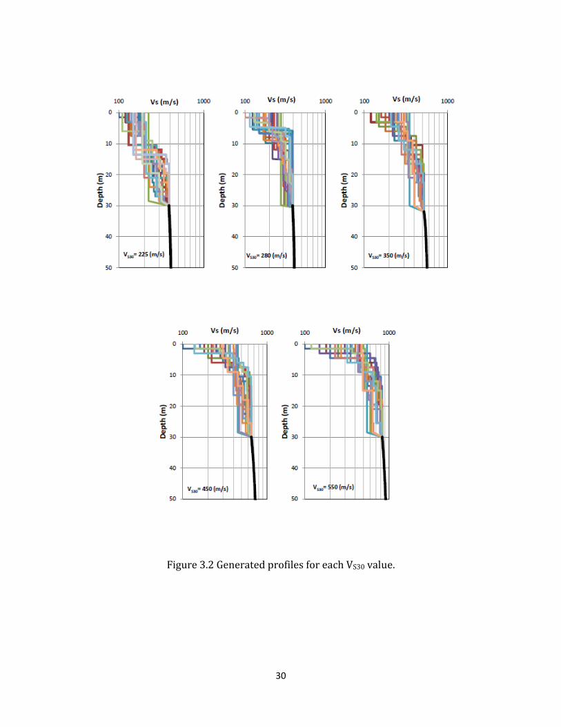
The top 50 m of all of the generated profiles, along with the baseline profile, for
each VS30 value are shown in Figure 3.2. In all the generated profiles, the velocity
increases with depth with no inversion in the shear wave velocity (i.e. an inversion
is when a smaller VS is found below a larger VS). The minimum shear wave velocity
is limited to 100 m/s in the generated profiles and for each VS30 the profiles all have
the same maximum VS as controlled by the baseline velocity profile at 30m.
0
25
50
75
100
125
150
0 200 400 600 800 1000
Dep
th (m
)
Vs(m/s)
VS30=225&280 m/s
VS30=350 m/s
VS30=450 m/s
VS30=550 m/s
30 m

29
In addition to the shear wave velocity profile, the unit weight and the shear
modulus reduction and damping curves of the soil layers are required for site
response analysis. The shear modulus reduction and damping curves describe the
variation of the shear modulus and damping ratio with shear strain, and represent
the nonlinear properties of the soil. For each of the profiles, the same unit weights,
as well as shear modulus reduction and damping curves are used. The Darendeli
(2001) model is used to develop the modulus reduction and damping curves as a
function of mean effective stress (σ’0), Plasticity Index (PI), and over-consolidation
ratio (OCR). In this study PI and OCR are taken to be 10 and 1.0, respectively, for all
layers. To model the stress dependence, the 150 m of soil is split into 5 layers
(Figure 3.3) and the nonlinear property curves computed for the mean effective
stress at the middle of each layer. The resulting shear modulus reduction and
damping curves for each layer are shown in Figure 3.4. Generally, the shear modulus
reduction curve shifts up as mean effective stress increases, while the damping
curve shifts down.
30
Figure 3.2 Generated profiles for each VS30 value.

31
Figure 3.3 Soil layers used to determine the nonlinear soil property curves used in the analyses.
Figure 3.4 Shear modulus and damping curves used in the analyses (PI=10, OCR=1.0).
0
0.2
0.4
0.6
0.8
1
0.0001 0.001 0.01 0.1 1 10
G/G
max
Strain (%)
Layer a
Layer b
Layer c
Layer d
Layer e
0
5
10
15
20
25
0.0001 0.001 0.01 0.1 1 10
Dam
pin
g R
atio
(%
)
Strain (%)
Layer a
Layer b
Layer c
Layer d
Layer e
γ= 8 kN/m3 σ’0=0.59 atm
γ= 8 kN/m3 σ’0=1.4 atm
γ= 9 kN/m3 σ’0=2.7 atm
γ= 2 kN/m3 σ’0=4.9 atm
γ= 21 kN/m3 σ’0=8.0 atm
Layer a
Layer b
Layer c
Layer d
Layer e
0.00 (m)
15.0 (m)
30.0 (m)
60.0 (m)
100.0 (m)
150.0 (m)
Bedrock

32
3.3 Input Motions
The Random Vibration Theory (RVT) approach to equivalent-linear site response
analysis is used. The RVT method allows equivalent linear site response to be
calculated without the need to specify an input time series. Rather, the RVT method
specifies the Fourier Amplitude Spectrum (FAS) of the input motion and propagates
the FAS through the soil column using frequency domain transfer functions. The
program Strata can generate input FAS from a specified input response spectrum or
through seismological theory. For this study, the input motion is specified by
seismological theory using the single-corner frequency, ω2 point source model
(Brune 1970). This model and its use in RVT predictions of ground shaking is
discussed further in Boore (2003). To specify the input motion, the earthquake
magnitude, site-to-source distance, and source depth is provided by user. The other
seismological parameters in the model (Table 3.1) are taken from Campbell (2003)
and represent typical values for the Western US region.
To consider the nonlinear behavior, the analyses are performed at multiple input
intensities. Earthquake magnitude and site-source distance are varied to obtain
different input intensities from the seismological method. The magnitude, distance,
and depth corresponding used to generate the different input intensities are given
in Table 3.2 along with the resulting PGArock. The range of magnitudes is between
6.5 and 7.8 while the range of Epicentral distances is 6 to 180 km. The resulting

33
PGArock values are from 0.01g to 1.5g and the resulting rock response spectra are
shown in Figure 3.5.
Figure 3.5 Response spectra of RVT input motions.
Table 3.1 Seismological parameters used in single-corner frequency, ω2 point source model.
Parameter Value
Stress drop, Δσ (bar) 100
Path attenuation, Q(f)=afb
Coefficient a 180
Power b 0.45
Site attenuation,κ0 (sec) 0.04
Density,ρ (g/cm3) 2.8
Shear-wave velocity of crust (km/sec) 3.5
0.001
0.01
0.1
1
10
0.01 0.1 1 10
Sa (
g)
Period (s)
PGAr=0.01g
PGAr=0.05g
PGAr=0.09g
PGAr=0.16g
PGAr=0.22g
PGAr=0.3g
PGAr=0.4g
PGAr=0.5g
PGAr=0.75g
PGAr=0.9g
PGAr=1.1g
PGAr=1.5g

34
Table 3.2 Corresponding magnitude, distance, and depth to input intensities.
Magnitude Distance
(km) Depth (km)
PGArock
7.0 180 3 0.01 g 7.0 68 3 0.05 g 7.0 40 3 0.09 g 6.5 20 3 0.16 g 7.0 21 3 0.22 g 7.0 16 3 0.3 g 7.0 21 3 0.4 g 7.0 10 3 0.5 g 7.0 7 3 0.75 g 7.6 9 3 0.9 g 7.5 7 3 1.1 g 7.8 6 3 1.5 g
3.4 Site Characteristics
It is important to understand which spectral periods are influenced by the seismic
response of a site. One simple parameter that can be used to consider the period
range most affected by a site’s response is the site period, TS. TS is the period
corresponding to first mode and represents the entire VS profile from the rock to the
surface. The site period is estimated as:
TS = 4H/VS (3.1)
where H is the soil thickness and VS is the average shear wave velocity of the soil. VS
is computed from the travel time for a shear wave travelling through the entire soil
35
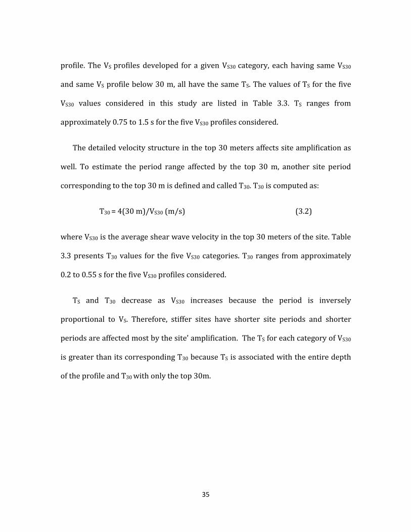
profile. The VS profiles developed for a given VS30 category, each having same VS30
and same VS profile below 30 m, all have the same TS. The values of TS for the five
VS30 values considered in this study are listed in Table 3.3. TS ranges from
approximately 0.75 to 1.5 s for the five VS30 profiles considered.
The detailed velocity structure in the top 30 meters affects site amplification as
well. To estimate the period range affected by the top 30 m, another site period
corresponding to the top 30 m is defined and called T30. T30 is computed as:
T30 = 4(30 m)/VS30 (m/s) (3.2)
where VS30 is the average shear wave velocity in the top 30 meters of the site. Table
3.3 presents T30 values for the five VS30 categories. T30 ranges from approximately
0.2 to 0.55 s for the five VS30 profiles considered.
TS and T30 decrease as VS30 increases because the period is inversely
proportional to VS. Therefore, stiffer sites have shorter site periods and shorter
periods are affected most by the site’ amplification. The TS for each category of VS30
is greater than its corresponding T30 because TS is associated with the entire depth
of the profile and T30 with only the top 30m.

36
Table 3.3 TS and T30 values for each VS30.
VS30 (m/s) TS (sec) T30 (sec)
225 1.54 0.53
280 1.45 0.43
350 1.10 0.34
450 0.87 0.27
550 0.72 0.22
To further investigate the period range in which the detailed velocity structure
in the top 30 m VS profile affects the response, 1D frequency domain transfer
functions are computed for different profiles. A transfer function describes the ratio
of the Fourier Amplitude Spectrum (FAS) of acceleration at any two points in the
soil column. Figure 3.6 plots the acceleration transfer functions between the surface
and the bedrock outcrop for three selected velocity profiles in the VS30=225 and 450
m/s categories. The soil properties are assumed linear elastic for calculating these
transfer functions. The transfer functions are plotted versus period in Figure 3.6 and
the corresponding periods for T30 and TS are indicated. For periods near TS, the
transfer functions of different profiles in the same VS30 category are very similar
because the transfer function in this period range is controlled by the full VS profile.
Starting at periods around T30 and at periods shorter than T30, the transfer functions
vary significantly between the different profiles even though they have the same
VS30. This variability in the transfer function illustrates the influence of the details of

37
the top 30 m VS profile in this period range. It can be concluded that the details of
the top 30 m of a site are important at periods shorter than T30. As a result, the
period range influenced by the top 30 m depends on VS30 (since T30 is VS30
dependent). Because the transfer functions in Figure 3.6 are for linear-elastic
conditions, an additional consideration will be the influence of input intensity and
soil nonlinearity. As the input intensity increases the soil becomes more nonlinear,
both TS and T30 will shift to long periods. As a result, the period range affected by
the top 30 m will increase to longer periods as input intensity increases.
0.1 1 10
Period (s)
0
1
2
3
4
5
Tra
nsfe
rF
un
cti
on
VS30=225 m/s
Linear Elastic Properties
TS
T30
0.1 1 10
Period (s)
0
1
2
3
4
5
Tra
nsfe
rF
unc
tio
n
VS30=450m/s
Linear Elastic Properties
TST30
Figure 3.6 Linear-elastic transfer function for 3 selected sites in VS30=225 and 450 m/s.

38
All the generated profiles in each category of VS30 have the same value of VS30 but
a different VS structure in the top 30 meters. Several parameters are identified from
the velocity profiles as candidates that affect the computed site amplification. These
parameters are Vmin, thVmin, depthVmin, MAXIR and Vratio. These parameters are
defined as:
Vmin is the minimum shear wave velocity in the VS profile
thVmin is the thickness of the layer with the minimum shear wave velocity
depthVmin is the depth to the top of the layer with Vmin
MAXIR is the maximum impedance ratio within the VS profile as defined
by the ratio of the VS of two adjacent layers (Vs,upper / Vs,lower)
Vratio is the ratio of the average shear wave velocity ( ) between 20 m
and 30 m to the average shear wave velocity in top 10 m. Vratio is defined
as:
(3.3)
Where
(3.4)
and
(3.5)

39
The concept of Vratio is similar to the impedance ratio for MAXIR, except that it
represents a more global impedance ratio in the top 30 m. It also has the advantage
of using information from a significant portion of the top 30 m of a profile, and it
also indicates how much the shear wave velocity increases in top 30 m. Vratio can
also indicate if a large scale velocity inversion occurs in the top 30 m when it takes
on values less than 1.0
To minimize the effect of soil nonlinearity both in studying the variability in AF
and the parameters that affect the variability, low levels of shaking are considered
first. To generalize the results of the study, larger level of shaking are then
considered.
3.5 Amplification at Low Input Intensities
3.5.1 Variability in Amplification Factors
Based on the existing empirical models of site amplification, all sites with the same
VS30 and Z1.0 should have the same AF. Figure 3.7 plots amplification factor versus
period for all of the generated sites for each of the VS30 categories subjected to the
lowest input intensity (0.01g). The amplification factors for a given VS30 are not
constant and show significant scatter. The amount of scatter (i.e. variability) varies
with VS30 and period. At smaller VS30, the variability in the amplification factors is
more significant. The period range in which the variability in AF is most significant

40
also depends on VS30. As VS30 increases, this period range decreases. At periods
greater than T30, less variability is observed. The period at which the maximum
variability in the AF occurs is also VS30 dependent. For VS30=225 m/s, the maximum
variability is observed at a spectral period of 0.3 sec. Stiffer sites (VS30=280 m/s and
350 m/s) display the maximum variability at a spectral period of 0.2 sec and the
stiffest sites (VS30=450 m/s and 550 m/s) display the maximum variability at a
spectral period of 0.1s.
To quantify the variability in AF, the standard deviation of ln(AF) at each period
for each category of VS30 is calculated. The standard deviation (σlnAF) is calculated
for the ln(AF) because ground motions are commonly assumed to be log-normally
distributed and to be consistent with its use in ground motion prediction equations
(see Section 2.2). Figure 3.8 shows the σlnAF values computed from the data in
Figure 3.7. σlnAF smaller than about 0.05 is considered small enough such that the
variability is minimal. The data in Figure 3.8 show that σlnAF is greater than 0.05 at
periods less than about T30 for each VS30, which is consistent with the observations
from the transfer functions. Additionally, the values of σlnAF are VS30 dependent, with
sites with smaller VS30 producing larger values of σlnAF.

41
0.01 0.1 1T (sec)
0.1
1
10
Am
plif
icat
ion
Fact
or
(AF
)
VS30=225 m/s
PGArock=0.01g
T30
0.01 0.1 1T (sec)
0.1
1
10
Am
pli
ficat
ion
Fact
or
(AF
)
VS30=280 m/s
PGArock=0.01g
0.01 0.1 1T (sec)
0.1
1
10
Am
plif
icat
ion
Fac
tor
(AF)
VS30=350 m/s
PGArock=0.01g
T30
0.01 0.1 1T (sec)
0.1
1
10
Am
plif
icat
ion
Fac
tor
(AF)
VS30=450 m/s
PGArock=0.01g
T30
0.01 0.1 1T (sec)
0.1
1
10
Am
plif
icat
ion
Fac
tor
(AF)
VS30=550 m/s
PGArock=0.01g
T30
Figure 3.7 Amplification factor vs. period for all the generated profiles, PGArock=0.01g.

42
0.01 0.1 1 10
T (sec)
0
0.1
0.2
0.3
0.4
0.5
lnA
F
VS30=225 m/s
PGArock=0.01g
T30
0.01 0.1 1 10
T (sec)
0
0.1
0.2
0.3
0.4
0.5
lnA
F
VS30=280 m/s
PGArock=0.01g
T30
0.01 0 .1 1 10
T (sec)
0
0.1
0.2
0.3
0.4
0.5
lnA
F
VS30=350 m/s
PGArock=0.01g
T30
0.01 0 .1 1 10
T (sec)
0
0.1
0.2
0.3
0.4
0.5
lnA
F
VS30=450 m/s
PGArock=0.01g
T30
0.01 0.1 1 10
T (sec)
0
0.1
0.2
0.3
0.4
0.5
lnA
F
VS30=550 m/s
PGArock=0.01g
T30
Figure 3.8 σlnAF versus period for all the generated profiles, PGArock=0.01g.

43
3.5.2 Identification of site parameters that explain
variation in AF
The identification of the site parameters that explain the variability in AF is initiated
by relating the data in Figure 3.7 to various site parameters. Considering the periods
that have large σlnAF values, only periods of 0.1 s, 0.2 s, and 0.3 s will be considered
here.
To investigate the site parameters that explain the variability in AF, the
difference between each ln(AF) and the average ln(AF) for a given period, input
intensity, and VS30 is considered. This difference represents the residual and is
defined as:
Residual = ln(AF) - μlnAF (3.6)
where ln(AF) represents the AF for a single VS profile with a given VS30 and μlnAF is
the average ln(AF) for all sites with the same VS30 (Figure 3.9).
The residual measures the difference between a specific value of AF and the
average value of AF for all sites with the same VS30 for a given period and input
intensity. If a trend is observed between the calculated residuals and a site
parameter, then that parameter influences site amplification and potentially should
be included in predictive models for AF to reduce its variability. As mentioned
previously, the minimum velocity in the profile (Vmin), the thickness of the layer with
the minimum velocity (thVmin), the depth to the layer with the minimum velocity

44
(depthVmin), the maximum impedance ratio (MAXIR), and Vratio are the site
characteristics that are considered.
.
Figure 3.9 Definition of calculated residual.
The first candidate parameter is Vmin. While the absolute value of Vmin is
important, its value relative to VS30 provides information about the range of
velocities within the top 30 meters. To consider the relative effect of Vmin, residuals
are plotted versus VS30/Vmin instead of Vmin. The minimum value of VS30/Vmin is 1.0,
which represents a site with constant velocity equal to VS30 in the top 30 meters.
Larger values of VS30/Vmin indicate smaller values of Vmin. Figure 3.10 shows the
residuals versus VS30/Vmin for all VS30 categories at a spectral period of 0.2 s and
PGArock=0.01g. For VS30≤350m/s the residuals generally increase with increasing
VS30/Vmin, while there is little influence of VS30/Vmin on the residuals for VS30=450

45
and 550 m/s. However, as shown in Figure 3.8, there is little variability in AF for
sites with VS30 = 450 and 550 m/s at this period (σlnAF~ 0.05).
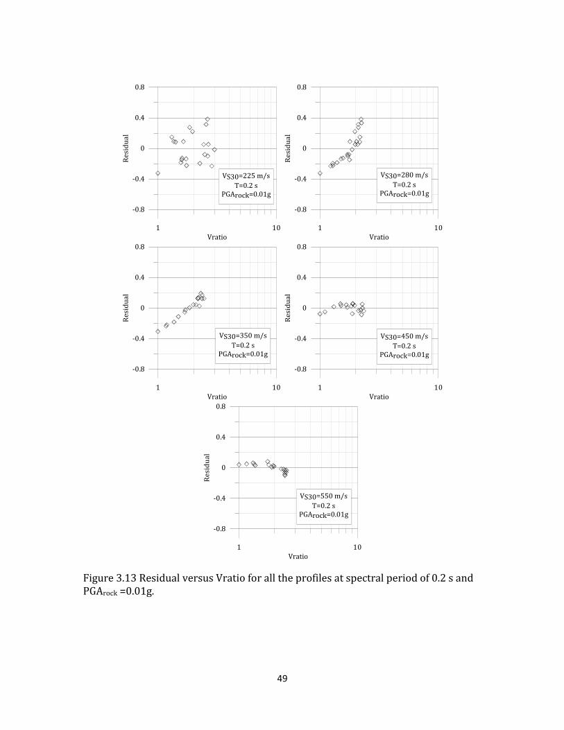
Other parameters that may influence AF are thVmin, MAXIR, depthVmin and Vratio.
In all the generated profiles in this study, the minimum velocity occurs at the ground
surface, such that all profiles have depthVmin equal to zero. Thus, this parameter
cannot be considered with the present dataset. The residuals versus thVmin, MAXIR,
and Vratio for a spectral period of 0.2 s and PGArock=0.01g are plotted in Figure 3.11,
3.12, and 3.13, respectively. The relationship between the residuals and thVmin is
quite weak (Figure 3.11). The relationship between the residuals and MAXIR
(Figure 3.12) is stronger, particularly for VS30 = 280 m/s and 350 m/s, but the
relationship is weak for VS30=225 m/s. The relationship between the residuals and
Vratio (Figure 3.13) is very strong for VS30 = 280 m/s and 350 m/s, and moderately
strong for VS30=225 m/s.

46
Figure 3.10 Residual versus VS30/Vmin for all the profiles at spectral period of 0.2 s and PGArock=0.01g.

47
Figure 3.11 Residual versus thVmin for all the profiles at spectral period of 0.2 s and PGArock=0.01g.

48
Figure 3.12 Residual versus MAXIR for all the profiles at spectral period of 0.2 s and PGArock =0.01g.
49
Figure 3.13 Residual versus Vratio for all the profiles at spectral period of 0.2 s and PGArock =0.01g.

50
Evaluating the relationship between the residuals and the four parameters,
Vratio is considered to best explain the variability in AF at this spectral period
because the relationship between that residuals and Vratio is stronger than the
three other parameters. Generally a linear relationship between the residual and
ln(Vratio) is observed. Considering σlnAF in Figure 3.8, the variability in AF is
significant for periods of 0.1s, 0.2s, and 0.3s for most of the VS30 values. Figures 3.14
and 3.15 show the residuals versus Vratio for PGArock=0.01g at spectral period of 0.1
s and 0.3 s respectively. A strong linear relationship is still observed between the
residuals and ln (Vratio). However, the intercept and slope of the linear fit is VS30
and period dependent.

51
1 10
Vratio
-0.8
-0.4
0
0.4
0.8
Re
sid
ua
l
VS30= 225 m/s
T=0.1 sPGAroc k=0.0 1g
1 10
Vratio
-0.8
-0.4
0
0.4
0.8
Re
sid
ua
l
VS3 0=2 80 m/s
T= 0.1 s
PGArock= 0.01 g
1 10
Vratio
-0.8
-0.4
0
0.4
0.8
Re
sid
ua
l
VS30 =35 0 m/s
T=0 .1 sPGArock= 0.01 g
1 10
Vratio
-0.8
-0.4
0
0.4
0.8
Re
sid
ua
l
VS30 =45 0 m/s
T=0 .1 sPGArock=0 .01g
1 10
Vratio
-0.8
-0.4
0
0.4
0.8
Re
sid
ua
l
VS30= 550 m/s
T=0.1 sPGAroc k=0.0 1g
Figure 3.14 Residual versus Vratio for all the profiles at spectral period of 0.1 s and PGArock=0.01g.

52
1 10
Vratio
-0.8
-0.4
0
0.4
0.8
Re
sid
ua
l
VS3 0=2 25 m/s
T= 0.3 sPGArock= 0.01 g
1 10
Vratio
-0.8
-0.4
0
0.4
0.8
Re
sid
ua
l
VS30 =28 0 m/s
T=0 .3 sPGArock=0 .01g
1 10
Vratio
-0.8
-0.4
0
0.4
0.8
Re
sid
ua
l
VS30 =3 50 m/s
T= 0.3 sPGAroc k=0.0 1g
1 10
Vratio
-0.8
-0.4
0
0.4
0.8
Re
sid
ua
l
VS3 0=4 50 m/s
T= 0.3 s
PGArock= 0.01 g
1 10
Vratio
-0.8
-0.4
0
0.4
0.8
Re
sid
ua
l
VS30= 550 m/s
T= 0.3 sPGAroc k=0.0 1g
Figure 3.15 Residual versus Vratio for all the profiles at spectral period of 0.3 s and PGArock=0.01g.

53
3.6 Amplification at Moderate Input Intensities
3.6.1 Variability in Amplification Factors
Soil layers show nonlinear behavior at larger input intensities because large strains
are induced which soften the soil and increase the material damping. Therefore,
amplification becomes a nonlinear function of input intensity at higher shaking
levels. To investigate the variability in AF at moderate intensities, the results for
PGArock=0.3g are presented.
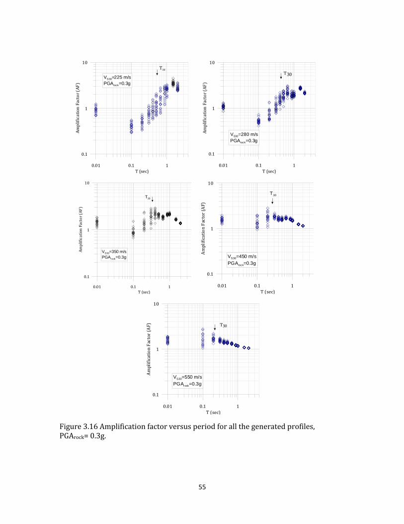
In Figure 3.16, AF versus period is shown for all the generated sites at
PGArock=0.3g. Comparing the AFs at each spectral period in Figure 3.16 with those in
Figure 3.7 for PGArock=0.01g, it is clear that there is an increase in amplification
variability. Figure 3.17 shows σlnAF versus period for each VS30 category for the AF
results shown in Figure 3.16. The largest values of σlnAF are observed at VS30=225
m/s. All the periods in this category of VS30 have significant variation in AF (i.e. σlnAF
>0.05). σlnAF is as large as 0.4 at T=0.66 s for this value of VS30. For all sites with VS30
≤ 5 m/s, σlnAF is significant at almost all periods considered ( 2.0 s). The
maximum value of σlnAF occurs at longer periods as VS30 decreases. Comparing each
VS30 category subjected to PGArock=0.3g to their corresponding profiles subjected to
PGArock= . g, the period range with σlnAF greater than 0.05 increases. The
maximum σlnAF occurs generally at longer periods for PGArock=0.3g than for

54
PGArock=0.01g. These observations indicate that the period range which is affected
by the details in the top 30 m VS profile increases as the shaking level increases.
55
0.01 0.1 1
T (sec)
0.1
1
10
Am
plif
icat
ion
Fact
or
(AF
)VS30=225 m/s
PGArock=0.3g
T30
0.01 0.1 1
T (sec)
0.1
1
10
Am
plif
icat
ion
Fact
or
(AF
)
VS30=280 m/s
PGArock=0.3g
T30
0.01 0.1 1
T (sec)
0.1
1
10
Am
plif
icat
ion
Fact
or
(AF
)
VS30=350 m/s
PGArock=0.3g
T30
0.01 0.1 1
T (sec)
0.1
1
10
Am
plif
icat
ion
Fac
tor
(AF)
VS30=450 m/s
PGArock=0.3g
T30
0.01 0.1 1T (sec)
0.1
1
10
Am
plif
icat
ion
Fac
tor
(AF)
VS30=550 m/s
PGArock=0.3g
T30
Figure 3.16 Amplification factor versus period for all the generated profiles, PGArock= 0.3g.

56
0.01 0.1 1 10T (sec)
0
0.1
0.2
0.3
0.4
0.5
lnA
FVS30=225 m/s
PGArock=0.3g
lnAF<0.05
T30
0.01 0.1 1 10
T (sec)
0
0.1
0.2
0.3
0.4
0.5
lnA
F
VS30=280 m/s
PGArock=0.3g
lnAF<0.05
T30
0.01 0.1 1 10T (sec)
0
0.1
0.2
0.3
0.4
0.5
lnA
F
VS30=350 m/s
PGArock=0.3g
lnAF<0.05
T30
0.01 0.1 1 10
T (sec)
0
0.1
0.2
0.3
0.4
0.5
lnA
F
VS30=450 m/s
PGArock=0.3g
lnAF<0.05
T30
0.01 0.1 1 10T (sec)
0
0.1
0.2
0.3
0.4
0.5
lnA
F
VS30=550 m/s
PGArock=0.3g
lnAF<0.05
T30
Figure 3.17 σlnAF versus period for all the generated profiles, PGArock=0.3 g.

57
3.6.2 Influence of site parameters on site amplification
Considering the periods of maximum σlnAF in Figure 3.17, the residuals are
investigated at periods of 0.2 s (period of maximum σlnAF for VS30=280 and 450 m/s),
0.66 s (period of maximum σlnAF for VS30=225 m/s) and T=1.0 s (period of large σlnAF
for VS30=225 m/s).
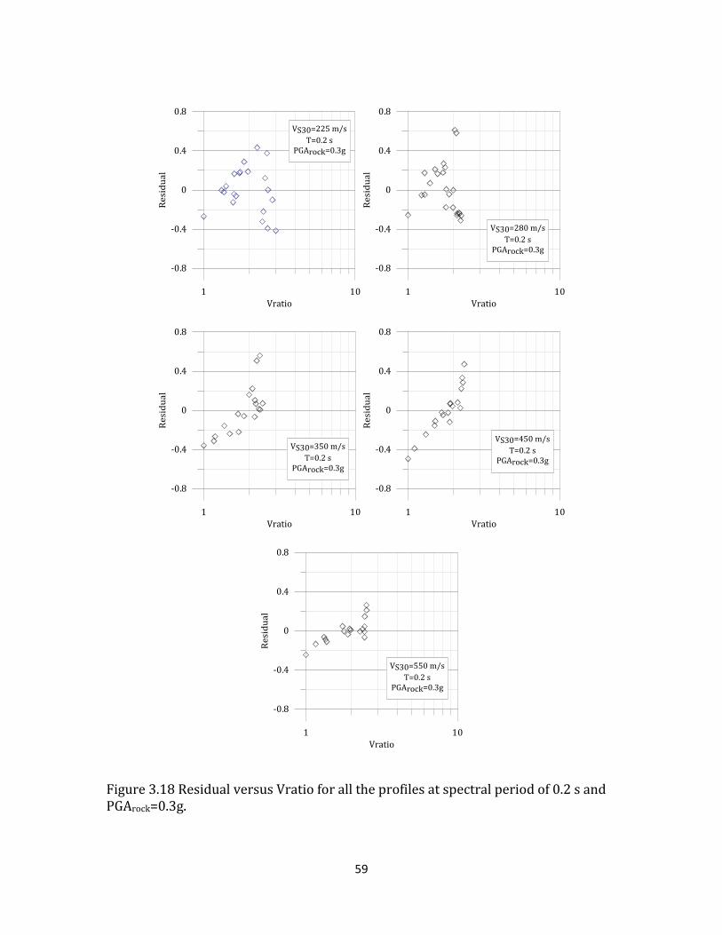
The residuals for the AF results for PGArock=0.3g at a spectral period of 0.2 s are
plotted versus Vratio in Figure 3.18. Generally, a linear trend between the residuals
and ln(Vratio) is observed, similar to the results for PGArock=0.01g. However, the
relationship appears to break down at small VS30 (i.e., 225 and 280 m/s) and larger
Vratio (i.e., 2 to 3). Figure 3.19 plots the velocity profiles over the top 30 m for four
VS30 = 225 m/s sites with Vratio around 2.5 but very high residuals (+0.4) and very
low residuals (-0.4) in Figure 3.18. The profiles with very low residuals have a thick,
soft layer (i.e., layer with VS 160 m/s and thickness > 10 m) with a large
impedance ratio (i.e., MAXIR) immediately below. The MAXIR is well above 2.0 for
these profiles, while the profiles with large residuals have MAXIR of between 1.5
and 1.7. The induced shear strains for the four profiles are also shown in Figure
3.19. The large MAXIR leads to significant shear strains, in excess of 2%, in the
layers above the depth of MAXIR. The rapid increase in strain across the impedance
contrast induces a rapid change in stiffness and damping which reduces the
amplification at high frequencies. While the sites with large residuals also
experience large strains (~ 1 to 1.5%), the increase in strain with depth is not as
58
rapid and that allow for more wave motion to travel through the soil. The data in
Figures 3.18 and 3.19 indicate that sites with very large MAXIR may experience very
large strains at moderate input motion intensities, which leads to smaller
amplification.
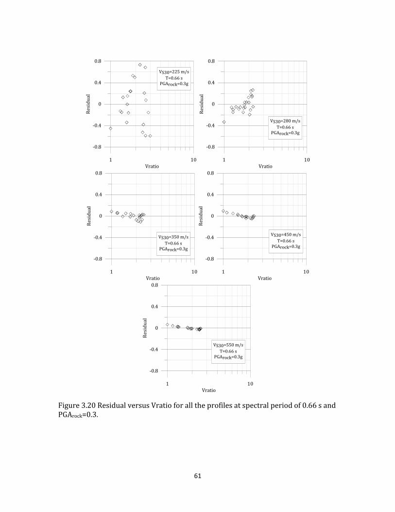
The maximum value of σlnAF for VS30=225 m/s occurs at T=0.66 s, while the value
of σlnAF is also significant at a spectral period of 0.66 s for VS30=280 m/s (Figure
3.17). Figure 3.20 shows the residuals versus Vratio for all the generated sites
subjected to PGArock=0.3g at spectral period of 0.66 s. For VS30 ≥ 5 m/s, the
residuals are almost zero at this spectral period because σlnAF is less than 0.05
(Figure 3.17). However a linear trend is generally observed between the residuals
and ln(Vratio) for the softer profiles (VS30=225 and 280 m/s). However, the data is
scattered for VS30=225 m/s and Vratio greater than about 2.3. These are the same
sites discussed in Figure 3.19, and the scatter is due to the large MAXIR and thick
soft layers in the profiles. Figure 3.21 shows the residual versus Vratio for T=1.0.
For VS30=225 m/s, a linear trend is observed between the residuals and ln(Vratio)
except for sites with Vratio greater than 2.3, as discussed previously. Generally at all
periods where the variability in amplification is significant (i.e., σlnAF >0.05), the
calculated residuals for these AF have a linear trend with ln(Vratio). However, there
are some profiles that break down this trend. These profiles tend to have a thick,
very soft layer near the surface that may be unrealistic.
59
Figure 3.18 Residual versus Vratio for all the profiles at spectral period of 0.2 s and PGArock=0.3g.

60
0 1 2 3Strain (%)
30
20
10
0
De
pth
(m)
Profiles with high residual
Profiles with low residual
Figure 3.19 VS profile for sites with Vratio ~ 2.5 but very low and very high residuals and the induced shear strains.
61
Figure 3.20 Residual versus Vratio for all the profiles at spectral period of 0.66 s and PGArock=0.3.

62
Figure 3.21 Residual versus Vratio for all the profiles at spectral period of 1.0 s and PGArock=0.3g.
63
3.7 Amplification at High Input Intensities
3.7.1 Variability in Amplification Factors
To study the effect of higher input intensity on site response, amplification factors
for the generated profiles at PGArock=0.9g are plotted versus period at Figure 3.22.
The variability in AF is significant (i.e σlnAF>0.05) at all periods for VS30=225, 280,
and 350 m/s and significant at periods less than or equal to 1.0 s for the stiffer sites
(VS30=450 and 550 m/s).
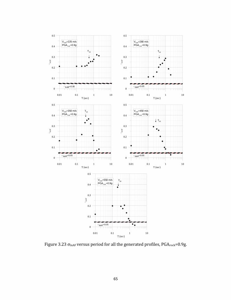
The calculated σlnAF of the AF values in Figure 3.22 are shown versus period in
Figure 3.23. Again, input intensity level affects the location of the maximum σlnAF.
The location of the maximum σlnAF moves to longer periods as the input intensity
increases. For example, for VS30=28 m/s the maximum σlnAF occurs at T=0.2 s for
PGArock= . g while the location of maximum σlnAF shifts to T=1.0 s for PGArock=0.9g.
While the location of the maximum σlnAF shifts to longer periods and the period
range of σlnAF ≥ . 5 expands with increasing input intensity, the maximum σlnAF
remains around 0.3 to 0.4 for both the moderate and high intensity input motions.

64
0.01 0.1 1T (sec)
0.1
1
10
Am
plif
icat
ion
Fact
or
(AF
)VS30=225 m/s
PGArock=0.9g
T30
0.01 0.1 1
T (sec)
0.1
1
10
Am
pli
ficat
ion
Fact
or
(AF
)
VS30=280 m/s
PGArock=0.9gT30
0.01 0.1 1T (sec)
0.1
1
10
Am
pli
ficat
ion
Fact
or
(AF
)
VS30=350 m/s
PGArock=0.9g
T30
0.01 0.1 1
T (sec)
0.1
1
10
Am
pli
fica
tion
Fact
or
(AF
)
VS30=450 m/s
PGArock=0.9g
T30
0.01 0.1 1T (sec)
0.1
1
10
Am
pli
ficat
ion
Fact
or
(AF
)
VS30=550 m/s
PGArock=0.9g
T30
Figure 3.22 Amplification factor versus period for all the generated profiles, PGArock= 0.9g.
65
0.01 0.1 1 10T (sec)
0
0.1
0.2
0.3
0.4
0.5
lnA
F
VS30=225 m/s
PGArock=0.9g
lnAF<0.05
T30
0.01 0.1 1 10
T (sec)
0
0.1
0.2
0.3
0.4
0.5
lnA
F
VS30=280 m/s
PGArock=0.9g
lnAF<0.05
T30
0.01 0.1 1 10T (sec)
0
0.1
0.2
0.3
0.4
0.5
lnA
F
VS30=350 m/s
PGArock=0.9g
lnAF<0.05
T30
0.01 0.1 1 10
T (sec)
0
0.1
0.2
0.3
0.4
0.5
lnA
F
VS30=450 m/s
PGArock=0.9g
lnAF<0.05
T30
0.01 0.1 1 10T (sec)
0
0.1
0.2
0.3
0.4
0.5
lnA
F
VS30=550 m/s
PGArock=0.9g
lnAF<0.05
T30
Figure 3.23 σlnAF versus period for all the generated profiles, PGArock=0.9g.
66
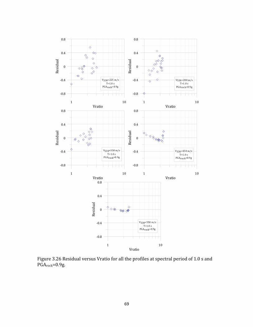
3.7.2 Influence of site parameters on site amplification
As investigated in previous sections, the Vratio of the VS profile affects amplification
at low and moderate shaking levels. In this section, the effect of this site parameter
under high level of shaking (0.9g) is examined. Considering the periods of the
maximum σlnAF in Figure 3.23, the residuals are investigated at periods of 0.2 s
(period of maximum σlnAF for VS30=450 and 550 m/s), 0.5 s (period of maximum σlnAF
for VS30=350 m/s), and 1.0 s (period of maximum σlnAF for VS30= 280 m/s).
Figure 3.24 shows the calculated residuals versus Vratio for all the generated
sites at spectral period of 0.2 s. A linear relationship between residuals and
ln(Vratio) is again observed. This relationship is now strong even for the larger VS30
sites (i.e., 550 m/s) because of soil nonlinearity. The residuals versus Vratio are
plotted at a spectral period of 0.5 s in Figure 3.25. The maximum σlnAF occurs at T=
0.5 s for VS30= 5 m/s and σlnAF is significant for all the other VS30 values at this
period. The linear trend between the residuals and ln(Vratio) is strong for VS30≤ 350
m/s. At longer spectral periods (1.0 s) as shown in Figure 3.26, the same trend as
that of for spectral period of 0.5 s is observed between residuals and ln(Vratio).

67
1 10Vratio
-0.8
-0.4
0
0.4
0.8
Re
sid
ua
l
VS30=225 m/s
T=0.2 sPGArock=0.9g
1 10
Vratio
-0.8
-0.4
0
0.4
0.8
Re
sid
ua
l
VS30=280 m/s
T=0.2 s
PGArock=0.9g
1 10Vratio
-0.8
-0.4
0
0.4
0.8
Re
sid
ua
l
VS30=350 m/s
T=0.2 sPGArock=0.9g
1 10
Vratio
-0.8
-0.4
0
0.4
0.8
Re
sid
ua
l
VS30=450 m/s
T=0.2 sPGArock=0.9g
1 10Vratio
-0.8
-0.4
0
0.4
0.8
Re
sid
ua
l
VS30=550 m/s
T=0.2 sPGArock=0.9g
Figure 3.24 Residual versus Vratio for all the profiles at spectral period of 0.2 s and PGArock=0.9g.

68
1 10
Vratio
-0.8
-0.4
0
0.4
0.8
Res
idu
al
VS3 0=2 25 m/s
T= 0.5 sPGArock=0 .9g
1 10
Vratio
-0.8
-0.4
0
0.4
0.8
Re
sid
ua
l
VS30= 280 m/s
T=0.5 s
PGArock =0.9 g
1 10
Vratio
-0.8
-0.4
0
0.4
0.8
Re
sid
ua
l
VS30 =35 0 m/s
T=0 .5 sPGAroc k=0.9 g
1 10
Vratio
-0.8
-0.4
0
0.4
0.8
Re
sid
ua
l
VS30= 450 m/s
T=0.5 sPGArock= 0.9g
1 10
Vratio
-0.8
-0.4
0
0.4
0.8
Re
sid
ua
l
VS30= 550 m/s
T=0.5 sPGArock= 0.9g
Figure 3.25 Residual versus Vratio for all the profiles at spectral period of 0.5 s and PGArock=0.9g.
69
1 10
Vratio
-0.8
-0.4
0
0.4
0.8
Re
sid
ua
l
VS30= 225 m/s
T=1.0 sPGArock= 0.9g
1 10
Vratio
-0.8
-0.4
0
0.4
0.8
Re
sid
ua
l
VS30 =28 0 m/s
T=1 .0 s
PGAroc k=0.9 g
1 10
Vratio
-0.8
-0.4
0
0.4
0.8
Re
sid
ua
l
VS3 0=3 50 m/s
T= 1.0 sPGArock=0 .9g
1 10
Vratio
-0.8
-0.4
0
0.4
0.8
Re
sid
ua
l
VS30 =45 0 m/s
T=1 .0 sPGAroc k=0.9 g
1 10
Vratio
-0.8
-0.4
0
0.4
0.8
Re
sid
ua
l
VS30= 550 m/s
T=1.0 sPGArock= 0.9g
Figure 3.26 Residual versus Vratio for all the profiles at spectral period of 1.0 s and PGArock=0.9g.

70
3.8 Summary
Ninety-nine profiles are manually generated using five baseline profiles. The
generated profiles from each baseline profile have the same average shear wave
velocity in top 30 m, the same velocity structure at depths greater than 30m, and the
same depth to bedrock. Site response analyses are performed using the equivalent
linear approach using the site response program Strata (Kottke and Rathje 2008).
The site amplification factors computed for the generated profiles are studied and
the variability in computed amplification investigated.
At low input intensity, sites with the same average shear wave velocity and
depth to rock but a different structure in the VS profile in the top 30 meters have
different amplification factors at some periods. These periods are correlated to T30.
The variability in the amplification factors at these periods indicates that the
detailed velocity structure in the top 30 meters of a VS profile influences the
computed AF. As input intensity increases, the period range affected by the top 30
meters increases.
The parameters Vmin, thVmin, depthVmin, MAXIR and Vratio are considered to
explain the variability in amplification factors. The parameter Vratio is identified as
the parameter that most strongly influences the computed amplification. A linear
relationship is observed between residuals and ln(Vratio). Residuals versus
ln(Vratio) plots for different VS30 and at different periods show that the effect of

71
Vratio on amplification is VS30 and period dependent. To generalize the findings of
this chapter, a suite of fully randomized velocity profiles will be analyzed.

72
Chapter 4
Statistical Generation of Velocity
Profiles
4.1 Introduction
As discussed in the previous chapter Vratio can help explain the variability in the
computed amplification factors for sites with the same average shear wave velocity
in top 30 meter (VS30) and depth to engineering rock (Z1.0). To generalize the effect
of Vratio to a wider range of sites, the seismic response of sites with a wide range of
velocity profiles is assessed and used to develop predictive models for site
amplification that include Vratio. The site response program Strata (Kottke and
Rathje, 2008) can generate hypothetical velocity profiles using Monte Carlo
simulations, and can also statistically vary layer thickness, nonlinear soil properties,
and depth to the bedrock. In this study four hundred hypothetical velocity profiles
are generated using Strata and their seismic responses are used to develop the site

73
amplification model. This chapter describes the generation of the velocity profiles,
while the next chapters describe the development of the site amplification model.
4.2 Development of Randomized Velocity Profiles
for Site Response Analysis
4.2.1 Modeling Variations in Site Properties
A soil profile consists of discrete layers that describe the variation of soil properties
with depth. In seismic site response analysis, each soil layer is characterized by a
thickness, mass density, shear wave velocity, and nonlinear properties (i.e., G/Gmax
vs. shear strain, and D vs. shear strain).
The site response program Strata (Kottke and Rathje 2008) uses Monte Carlo
simulations to develop different potential realizations of the site properties. The
goal of a Monte Carlo simulation is to estimate the statistical properties of the
response of a complex system. To achieve this goal, each of the properties of the
system is selected from defined statistical distribution and the response of the
system is computed. The response is computed for many realizations of site
properties and the calculated response from each realization is then used to
estimate the statistical properties of the system’s response. Monte Carlo
74
simulations require that each of the components in the system has a complete
statistical description.
The Monte Carlo randomization feature in Strata can randomize layer
thickness, the shear wave velocity of a layer, the nonlinear soil properties of a
layer, and the depth to bedrock. In this study, layer thicknesses, shear wave
velocity, and depth to bedrock are randomized; nonlinear properties are not.
Strata uses the statistical models developed by Toro (1995) to randomize the layer
thicknesses and associated shear wave velocities. In this approach, layer
thicknesses are first generated and then shear wave velocities are assigned to each
layer.
Layering is modeled as a Poisson process, which is a stochastic process with the
event occurring at a given rate (λ). For a homogeneous Poisson process this rate is
constant, while for a non-homogeneous Poisson process the rate of occurrence
varies. For the layering problem, the event is a layer interface and its rate is defined
in terms of the number of layer interfaces per meter. The rate of interface
occurrence is depth dependent (i.e., thinner layers tend to occur near the surface,
thicker layers tend to occur at depth), thus a non-homogeneous Poisson process is
used. Toro (1995) developed a depth-dependent layering rate model using the layer
thicknesses measured at 557 sites, mostly from California. The resulting model of
depth-dependent layering rate is shown in Figure 4.1. Note that the rate varies from
0.22 (per meter) at the ground surface (i.e., average layer thickness = 1/ λ = 4.5 m)

75
to 0.05 (per meter) at a depth 50 m (i.e., average layer thickness = 20 m) to 0.02
(per meter) at a depth of 200 m (i.e., average layer thickness = 50 m).
Figure 4.1 Variation of layer interface occurrence rate with depth (Toro 1995).
After developing the layering profile (i.e., layer thicknesses) using the non-
homogeneous Poisson process, a shear wave velocity is assigned to each layer. In
the Toro (1995) model, the shear wave velocity at mid-depth of the layer is
described by the log-normal distribution. The log-normal distribution is used based
on statistical investigation of shear wave velocity data from the same 557 sites used
in developing the layering model. The log-normal distribution is described by the
median shear wave velocity (i.e., the average of ln(Vs)) at mid-depth of the layer and
the standard deviation of the natural logarithm of the shear wave velocity (lnVs).

76
The median shear wave velocity for the layer is taken from a user-specified baseline
velocity profile for the site, at the depth of the layer. The lnVs is assigned by the
user to model a specific amount of variability. Given the baseline shear wave
velocity for layer i (Vs,o(i), assumed to represent the mean in logarithmic space), the
standard deviation of the natural logarithm of Vs (lnVs), and a random standard
normal variable for layer i (Zi), the shear wave velocity of layer i (Vs(i)) can be
computed as (Toro 1995):
(4.1)
The key issue is then the selection of the values of Zi for each layer. Some
researchers have assumed that Zi values are perfectly correlated between layers
(McGuire et al. 1989, Toro et al. 1992), while others have assumed zero correlation
(Costantino et al. 1991). Neither of these assumptions is consistent with velocity
data and they represent extreme conditions (i.e., perfect correlation vs. statistical
independence). Toro (1995) developed a model for the interlayer correlation of Zi
based on analysis of the same 557 shear wave velocity profiles previously discussed.
In this model, the standard normal variable for the surface layer (Z1, i = 1) is
independent of all other layers and defined as:
(4.2)
where is a random normal variable with zero mean and unit standard deviation.
Zi is correlated with the layer above it using (Toro 1995):

77
(4.3)
where Zi-1 is the standard normal variable of the previous layer, is a new normal
random variable with zero mean and unit standard deviation, and is the
interlayer correlation coefficient. Toro (1995) modeled the interlayer correlation
as depth (d) and layer thickness (t) dependent:
(4.4)
where is the depth-dependent component of the correlation coefficient and
is the thickness-dependent component of the correlation coefficient. These
correlation coefficients are defined as (Toro 1995):
(4.5)
(4.6)
where , , , , and are model parameters.
Toro (1995) developed median shear wave velocity profiles for different site
classes (i.e., ranges in VS30 that are incorporated in the building code) for use in
developing randomized velocity profiles for generic site conditions. Toro (1995)
also developed estimates of lnVs and inter-layer correlation coefficient model
parameters for site classes of VS30 > 760 m/s, 360-760 m/s, 180-360 m/s, and <
180 m/s.
78
The depth to bedrock can be modeled using either a uniform, normal, or log-
normal distribution. The statistical properties of the distribution are entered by
the user.
4.2.2 Baseline Profiles
The Monte Carlo simulation feature in the program Strata is used to generate
generic site profiles for use in site response analysis. As discussed in the previous
section, Monte Carlo simulations require a median shear wave velocity profile and
lnVs. The median shear wave velocity profiles are called baseline profiles in this
study. Four baseline profiles with VS30 equal to 200, 250, 400, and 550 m/s are used
to generate a total of four hundred soil profiles. The developed baseline shear wave
velocity profiles are shown in Figure 4.2. These baseline velocity profiles are
developed based on the velocity profiles presented by Toro (1995) for different site
classes. The developed profiles by Toro (1995) are modified in this study to achieve
the desired VS30 for each baseline profile. The minimum velocity at the surface varies
between about 175 and 400 m/s in the baseline profiles. The baseline profiles with
VS30 of 200 and 250 m/s reach their maximum shear wave velocities of 750 m/s and
890 m/s, respectively, at a depth of 400 m. The stiffer baseline profiles reach VS
equal to 1,000 m/s at shallower depths (150 m for VS30 of 550 m/s and 300 m for
VS30 of 400 m/s). The site class dependent values of lnVs developed by Toro (1995)
are used in generating the velocity profiles (Table 4.1).
79
Generic layering is developed for the site profiles using the non-homogenous
layering model of Toro (1995). Depth to bedrock is varied using a uniform
distribution. The minimum and maximum depths used for the uniform distribution
are specified differently for each baseline velocity profile because each profile
encounters rock-like velocities (~ 750 to 1000 m/s) at different depths. The
minimum and maximum depths used are listed in Table 4.1 for each baseline profile.
The shear wave velocity of the half-space below the velocity profile is specified as
1,000 m/s. Velocities are assigned to each layer using the inter-layer correlation
model of Toro (1995). The depth and thickness-dependent model for from Toro
(1995) is used. The predicted from Toro (1995) is plotted versus depth for
thicknesses of 5 m, 20 m, and 50 m in Figure 4.3 for site class VS30 = 180-360 m/s.
This is the site class that is associated with the VS30 values of two of the baseline
profiles. As shown in Figure 4.3, for a given thickness, the interlayer correlation
increases with depth and at the depth of 200 m approaches 1.0 for this site class. It
is also observed that thicker layers generally have a smaller interlayer correlation
coefficient. In generating the velocity profiles, the shear wave velocity of layers is
not allowed to exceed 1000 m/s nor go below 100 m/s.
While the nonlinear properties are not varied in the Monte Carlo simulation,
modulus reduction and damping curves are assigned to each layer. The Darendeli
(2001) model is used to develop the modulus reduction and damping curves as a
function of mean effective stress (σ’0), Plasticity Index (PI), and over consolidation

80
ratio (OCR). In this study PI and OCR are taken to be 10 and 1.0, respectively, for all
layers. To model the stress dependence, nonlinear property curves are generated
for σ’0 equal to 0.59 atm, 1.4, atm, 2.7 atm, 4.9 atm, 8.0 atm, 15.7 atm, and 33.5 atm.
The appropriate curves are assigned to each layer of the baseline profile based on
the depth and a computed mean effective stress at the middle of each layer. The
thickness, unit weight, and mean effective stress considered for each layer are listed
in Table 4.2. The shear modulus reduction and damping curves used for each layer
are shown in Figure 4.4.
0 200 400 600 800 1000
Shear-wave Velocity (m/s)
500
400
300
200
100
0
De
pth
(m)
VS30
=200 (m/s)
VS30=250 (m/s)
VS30=400 (m/s)
VS30=550 (m/s)
Figure 4.2 Baseline shear wave velocity profiles.
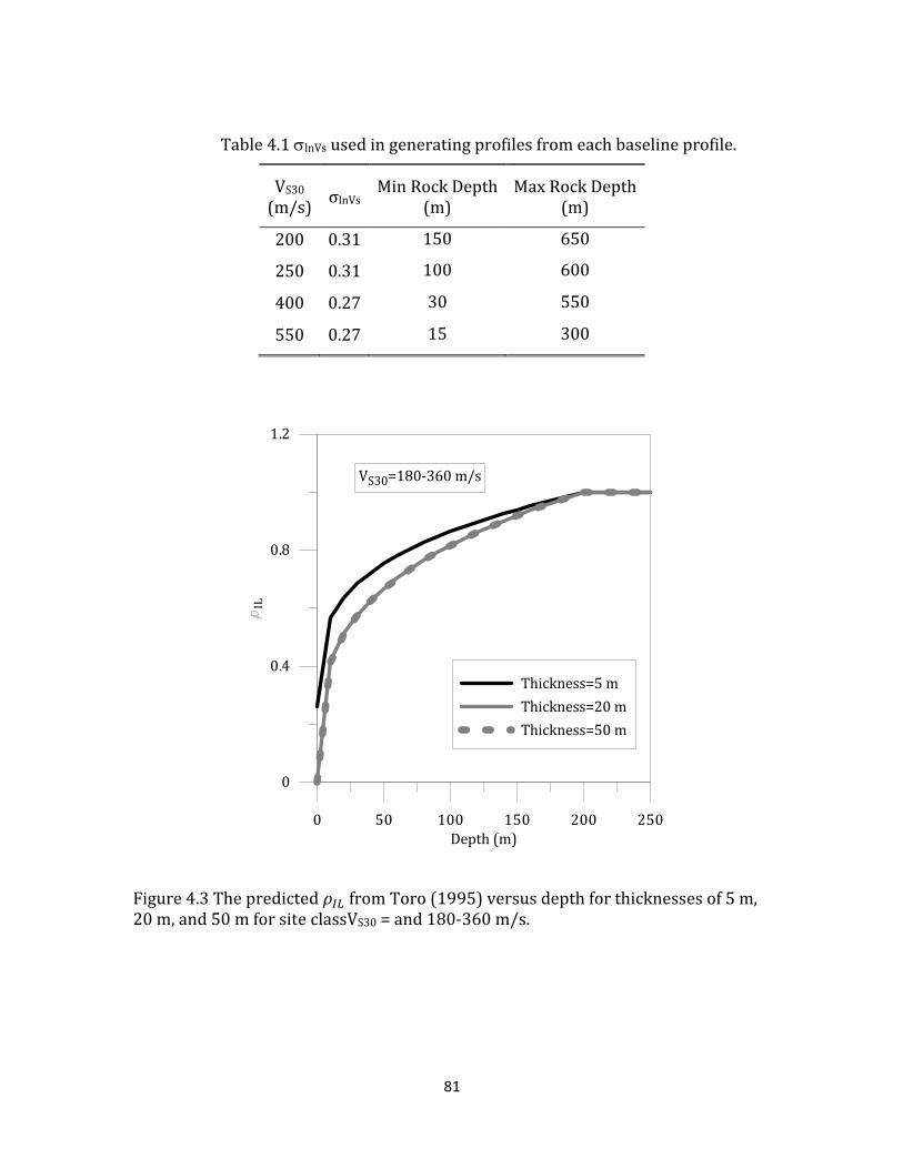
81
Table 4.1 lnVs used in generating profiles from each baseline profile.
VS30
(m/s) σlnVs
Min Rock Depth (m)
Max Rock Depth (m)
200 0.31 150 650
250 0.31 100 600
400 0.27 30 550
550 0.27 15 300
Figure 4.3 The predicted from Toro (1995) versus depth for thicknesses of 5 m, 20 m, and 50 m for site classVS30 = and 180-360 m/s.

82
Table 4.2 The thickness, unit weight, and mean effective stress considered for each layer.
Depth (m) Unit Weight
(kN/m3)
Mean Effective Stress
(atm)
0-15 18 0.59
15-30 18 1.4
30-60 19 2.7
60-100 20 4.9
100-150 21 8.0
150-300 22 15.7
300-600 22 33.5
0.0001 0.001 0.01 0.1 1 10Strain (%)
0
0.2
0.4
0.6
0.8
1
G/G
ma
x
'0=0.59 atm
'0=1.4 atm
'0=2.7 atm
'0=4.9 atm
'0=8.0 atm
'0=15.7 atm
'0=33.5 atm
0.0001 0.001 0.01 0.1 1 10
Strain (%)
0
5
10
15
20
25
Da
mp
ing
Ra
tio
(%)
'0=0.59 atm
'0=1.4 atm
'0=2.7 atm
'0=4.9 atm
'0=8.0 atm
'0=15.7 atm
'0=33.5 atm
Figure 4.4 Shear modulus and damping curves used in the analyses (PI=10, OCR=1.0).

83
4.2.3 Generated Shear Wave Velocity Profiles
Four hundred soil profiles are generated by the program Strata using the
information previously discussed. Examples of generated profiles from each
baseline profile are shown in Figures 4.5 and 4.6. Note that the VS30 for each
generated profile is different than the VS30 for the baseline profile. Each profile
generated from a single baseline profile has different layering and a different shear
wave velocity profile. While the baseline velocity profiles (Figure 4.2) vary
smoothly with depth, the generated profiles vary more irregularly (Figure 4.5, 4.6).
In some profiles, an inversion in the shear wave velocity occurs (i.e., the velocity
decreases with depth). The irregular pattern is more representative of a real site,
while the smooth baseline profiles represent the average over many different sites.
However, the average velocity profile for the generated sites for a given baseline
profile varies smoothly and matches well the baseline profile.
For each generated velocity profile, site characteristics such as the minimum
shear wave velocity, VS30, and the depth to bedrock are different. Various site
parameters, including the average shear wave velocity in top 30 m (VS30), the depth
to engineering rock (Z1.0), and Vratio (i.e., Vratio = VS20-30 / VS10, where VS20-30 is the
average shear wave velocity between depths 20 m and 30 m and VS10 is the average
shear wave velocity in top 10 m) are calculated for each generated profile.
Histograms showing the distribution of each of these site parameters are given in
Figure 4.7. VS30 in the generated profiles varies between 118 m/s and 818 m/s. The

84
VS30 values of the generated profiles are evenly distributed between 150 and 750
m/s, with fewer values less than 150 m/s or greater than 750 m/s. This range
indicates that the generated sites include a representative range of soft to stiff soil
profiles. The Z1.0 values of the generated profiles range from 16 m to 640 m.
Because softer sites with small VS30 tend to be found in deeper alluvial valleys, there
is a relationship between VS30 and Z1.0. As shown in Figure 4.8 for the generated
profiles in this study, the softest sites are associated with the largest values of Z1.0.
The histograms in Figure 4.7 show that Vratio varies from 0.56 to 2.76 in the
generated profiles. Profiles with Vratio less than 1.0 have VS10 greater than VS20-30,
indicating that the shear wave velocity generally does not increase with depth in the
top 30 m. In these cases an inversion in the velocity occurs. In 11% of the
generated profiles Vratio is less than one. Large values of Vratio indicate a
significant increase in shear wave velocity within the top 30 m.
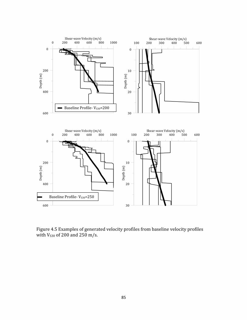
85
0 200 400 600 800 1000Shear-wave Velocity (m/s)
600
400
200
0
De
pth
(m)
100 200 300 400 500 600Shear-wave Velocity (m/s)
30
20
10
0
De
pth
(m)
0 200 400 600 800 1000Shear-wave Velocity (m/s)
600
400
200
0
De
pth
(m)
100 200 300 400 500 600Shear-wave Velocity (m/s)
30
20
10
0
De
pth
(m)
Figure 4.5 Examples of generated velocity profiles from baseline velocity profiles with VS30 of 200 and 250 m/s.
Baseline Profile- VS30=200
(m/s)
Baseline Profile- VS30=250
(m/s)
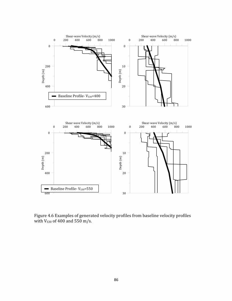
86
0 200 400 600 800 1000Shear-wave Velocity (m/s)
600
400
200
0D
ep
th(m
)
0 200 400 600 800 1000Shear-wave Velocity (m/s)
30
20
10
0
De
pth
(m)
0 200 400 600 800 1000Shear-wave Velocity (m/s)
600
400
200
0
De
pth
(m)
0 200 400 600 800 1000Shear-wave Velocity (m/s)
30
20
10
0
De
pth
(m)
Figure 4.6 Examples of generated velocity profiles from baseline velocity profiles with VS30 of 400 and 550 m/s.
Baseline Profile- VS30=400
(m/s)
Baseline Profile- VS30=550
(m/s)

87
Figure 4.7 Distiribution of VS30, Z1.0, and Vratio of the generated soil profiles.
0
20
40
60
80
100
120
No
. of
Site
s
VS30 (m/s)
0
20
40
60
80
100
120
<150 150-300 300-400 <400
No
. of
Site
s
Z1.0 (m)
0
20
40
60
80
100
120
<1.0 1.0-1.2 1.2-1.4 1.4-1.6 1.6-1.8 1.8-2.0 >2.0
No
. of
Site
s
Vratio

88
Figure 4.8 Relation between Z1.0 and VS30.
4.3 Approach to Development of Amplification
Model
The form of empirical site amplification models typically includes two components;
a linear elastic component and a nonlinear component. The linear elastic
component represents amplification under linear elastic (LE) soil conditions (i.e.,
low intensity shaking), while the nonlinear component (NL) includes the effects of
soil nonlinearity at high intensity shaking. These amplification factors (AF) are
generally multiplicative (additive in logarithmic space), which can be written as:
ln (AF)=ln(AF)LE+ ln(AF)NL (4.7)

89
The amplification model is developed separately for each period in the response
spectrum.
The linear elastic component can be derived from the computed amplification
for low intensity input motions. In this study, computed amplification factors from
input motions with a rock input PGA of 0.01g are used to develop the linear elastic
AF model. Computed amplification factors from larger intensity input motions are
used to develop the nonlinear component of the AF model. As discussed earlier,
equivalent-linear analysis using the RVT approach is used to compute the seismic
response of the generated profiles under a wide range of input intensities. In the
RVT approach, the input motion is described by a response spectrum, this response
spectrum is converted to a Fourier Amplitude Spectrum (FAS), the FAS is
propagated to the ground surface using the site frequency domain transfer function,
and the surface FAS is converted to an acceleration response spectrum. The ratio of
the surface response spectrum to the input response spectrum at each period
defines the AF for each period. The input motions are defined using seismological
source theory in which the earthquake magnitude, depth, and source-to-site
distance are specified by the user and Strata uses various seismological parameters
to define the input FAS and response spectrum. For this study, the magnitude and
distance are varied to obtain the desired input intensity levels. Table 4.3 lists the
magnitude, depth, and distance used to generate the 10 input intensity levels along
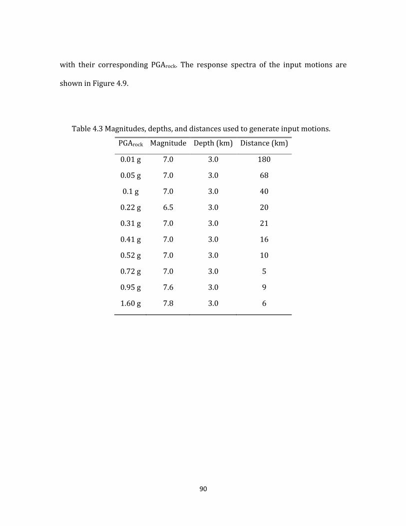
90
with their corresponding PGArock. The response spectra of the input motions are
shown in Figure 4.9.
Table 4.3 Magnitudes, depths, and distances used to generate input motions.
PGArock Magnitude Depth (km) Distance (km)
0.01 g 7.0 3.0 180
0.05 g 7.0 3.0 68
0.1 g 7.0 3.0 40
0.22 g 6.5 3.0 20
0.31 g 7.0 3.0 21
0.41 g 7.0 3.0 16
0.52 g 7.0 3.0 10
0.72 g 7.0 3.0 5
0.95 g 7.6 3.0 9
1.60 g 7.8 3.0 6

91
0.01 0.1 1 10
Period (s)
0.0001
0.001
0.01
0.1
1
10
Sa
(g)
PGArock=0.01g
PGArock=0.05g
PGArock=0.09g
PGArock=0.19g
PGArock=0.27g
PGArock=0.37g
PGArock=0.47g
PGArock=0.66g
PGArock=0.90g
PGArock=1.54g
Figure 4.9 Response spectra of RVT input motions.
After computing amplification factors for a range of sites subjected to a range of
input intensities, the AF values are used to develop the empirical amplification
model. A functional form for the model is developed and the model coefficients are
determined through a maximum likelihood regression.
Maximum likelihood estimation, identifies the regression coefficients for a model
that make the observed data most likely. The likelihood function (L) is written as:
(4.8)
where represents the parameters of the statistical model, represents the
observed values, n is the number of observations, and represents

92
the joint probability density function (pdf) of . Assuming that the are
independent and indentically distributed, the joint pdf can be written as:
(4.9)
It is often more convenient to use the logarithm of the likelihood (log-likelihood)
function:
(4.10)
The maximum likelihood method identifies the values of the statistical model
parameters that maximize the likelihood function.
When applying the maximum likelihood approach to regression, represent
observed values of the dependent variable and are the regression coefficients. In
developing the amplification model in this study, the maximum likelihood method is
implemented in Excel. The residual of each observation relative to the prediction is
computed, each residual is used to compute , and these values summed to
represent the log-likelihood. The Solver function in Excel is used to identify the
parameters that maximize the log-likelihood function
93
4.4 Summary
This chapter describes the development of randomized velocity profiles for site
response analysis. The model used in program Strata (Kottke and Rathje,2008) for
variation in site properties such as site depth, layer thickness, and nonlinear
properties of soils are discussed. Finally the statistically generated velocity profiles
and their correponding site parameters are presented and the approach for
developing the site amplification models is discussed.
In Chapteres 5 and 6, the linear and nonlinear components of the model will be
presented, respectively. In Chapter 7, the combined model will be presented.
94
Chapter 5
Models for Linear Site Amplification
5.1 Introduction
This chapter presents the development of the linear elastic component of the
predictive amplification model. The functional form is developed separately for
shorter periods (T < 1.0 s) and longer periods (T 1.0 s). At short periods the
amplification model includes the effects of VS30 and Vratio, while at long periods the
amplification model includes the effects of VS30 and Z1.0.
5.2 Linear Site Amplification (PGArock=0.01g)
The computed amplification factors (AF) for all the generated sites subjected to the
input motion with a PGArock of 0.01g are used to develop the model for linear elastic
amplification (i.e. ln(AF)LE). In Figures 5.1 and 5.2, the computed AFs are plotted
versus VS30 for spectral periods shorter and longer than 1.0 s, respectively. The data
95
in Figures 5.1 and 5.2 generally show that a decrease in VS30 results in an increase in
amplification, which is consistent with previous studies. At shorter periods,
amplification (i.e., T≤ .5) increases over the full S30 range. At longer periods (T =
5.0 and 10 s in Figure 5.2), the amplification stays close to 1.0 for a range of larger
VS30 values before beginning to increase at smaller VS30. The VS30 below which
amplification starts to increase is called Vref. Vref generally decreases as period
increases.
Linear elastic AF models developed previously and used in most ground motion
prediction equations (e.g., NGA models) incorporate a linear dependence between
lnAF and ln(VS30/Vref). This fit takes on the following functional form:
(5.1)
A maximum likelihood regression is used to fit equation (5.1) to the AF data at
each spectral period. Vref is fixed based on visual identification from the data (Table
5.1) because regressed values of Vref using the maximum likelihood method were
not consistent with the data. Figures 5.3 and 5.4 show the AF data again, along with
a linear fit from equation (5.1) in which parameters a1 and Vref are developed
separately for each period. These model parameters (a1 and Vref) and the resulting
standard deviation of the regression (σlnAF) are shown in Table 5.1. As shown in
Table 5.1, Vref is equal to 1000 m/s at short periods and then decreases as spectral
period increases beyond 0.5 s. The slope a1 is almost the same at short periods (~ -

96
0.45 for T 0.3 s), it gets larger in the middle periods (~ -0.5 to -0.7 for T = 0.5 to 2.0
s), and then it becomes smaller at long periods greater than 2.0 s. σlnAF ranges from
0.11 at PGA, then increases to 0.2 - 0.25 for periods between 0.2 and 1.0s, and then
decreases at the longest periods. Comparing the model predictions to the data in
Figures 5.3 and 5.4, it appears that a linear fit does not match the data appropriately,
particularly at shorter periods and smaller VS30. In these cases, a second-order
polynomial may fit the AF data better.

97
100 1000VS30 (m/s)
1
2
4
6
AF
PGA
100 1000VS30 (m/s)
1
2
4
6
AF
T=0.05 s
100 1000VS30 (m/s)
1
2
4
6
AF
T=0.1 s
100 1000VS30 (m/s)
1
2
4
6
AF
T=0.2 s
10 0 1000VS30 (m/s)
1
2
4
6
AF
T=0.3 s
100 1000VS30 (m/s)
1
2
4
6
AF
T=0.5 s
Figure 5.1 Amplification Factor versus VS30 for all generated profiles at short periods (T<1.0 s).

98
100 1000VS30 (m/s)
1
2
4
6
AF
T=1.0 s
100 1000VS30 (m/s)
1
2
4
6
AF
T=2.0 s
10 0 1000VS30 (m/s)
1
2
4
6
AF
T=5.0 s
100 1000VS30 (m/s)
1
2
4
6A
F
T=10.0 s
Figure 5.2 Amplification Factor versus VS30 for all generated profiles at long periods (T≥ . s).

99
100 1000VS30 (m/s)
1
2
4
6
AF
PGA
100 1000VS30 (m/s)
1
2
4
6
AF
T=0.05 s
100 1000VS30 (m/s)
1
2
4
6
AF
T=0.1 s
100 1000VS30 (m/s)
1
2
4
6
AF
T=0.2 s
100 1000VS30 (m/s)
1
2
4
6
AF
T=0.3 s
100 1000VS30 (m/s)
1
2
4
6
AF
T=0.5 s
Figure 5.3 Amplification Factor versus VS30 and linear fit to data for all generated profiles at short periods (T<1.0 s).
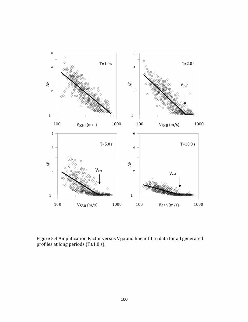
100
100 1000VS30 (m/s)
1
2
4
6
AF
T=1.0 s
100 1000VS30 (m/s)
1
2
4
6
AF
T=2.0 s
100 1000VS30 (m/s)
1
2
4
6
AF
T=5.0 s
100 1000VS30 (m/s)
1
2
4
6A
F
T=10.0 s
Figure 5.4 Amplification Factor versus VS30 and linear fit to data for all generated profiles at long periods (T≥ . s).
Vref Vref
Vref

101
Table 5. Coefficients and σlnAF of equation (5.1).
T(sec) a1 Vref
(m/s) σlnAF
PGA -0.49 1000 0.11
0.05 -0.47 1000 0.12
0.1 -0.44 1000 0.15
0.2 -0.42 1000 0.24
0.3 -0.46 1000 0.24
0.5 -0.52 1000 0.20
1.0 -0.62 850 0.20
2.0 -0.72 600 0.19
5.0 -0.46 500 0.18
10.0 -0.21 500 0.06
A second-order polynomial is considered for the relationship between lnAF
ln(VS30/Vref). This expression can be described as:
(5.2)
A maximum likelihood regression is used to fit equation (5.2) to the data at each
period. The same Vref values previously identified are used. The values of Vref, a1, a2,
and σlnAF for each period are listed in Table 5.2. The resulting second order

102
polynomials are shown in Figures 5.5 and 5.6, along with the linear fit and the AF
data. As compared with the linear fit from equation (5.1), the second order
polynomial better fits the data, particularly at smaller VS30. At periods longer than
1.0 s, the parameter a2 is close to zero indicating that a linear fit best represents the
data. Comparing the σlnAF of polynomial and linear fits, the polynomial fit decreases
σlnAF by 15 to 25% at periods shorter than about 0.5 s but does not significantly
decrease it at longer periods. Therefore, the linear fit appears to be appropriate for
periods greater than 0.5 s.

103
Figure 5.5 Amplification Factor versus VS30 along with linear and nonlinear fit to data for all generated profiles at short periods (T<1.0 s).

104
Figure 5.6 Amplification Factor versus VS30 along with linear and nonlinear fit to data for all generated profiles at long periods (T≥ ).

105
Table 5.2 Coefficients and σlnAF of equation (5.2).
T(sec) a1 a2 Vref
(m/s) σlnAF
(Eq 5.2) σlnAF
(Eq 5.1) %
Reduction PGA -0.7 -0.15 1000 0.09 0.11 18
0.05 -0.72 -0.17 1000 0.10 0.12 17
0.1 -0.79 -0.24 1000 0.11 0.15 27
0.2 -0.94 -0.36 1000 0.19 0.24 21
0.3 -0.93 -0.33 1000 0.20 0.24 17
0.5 -0.70 -0.12 1000 0.19 0.20 5
1.0 -0.49 0.09 850 0.19 0.20 5
2.0 -0.62 0.09 600 0.19 0.19 1
5.0 -0.26 0.08 500 0.20 0.18 -11
10.0 -0.12 0.09 500 0.07 0.06 -17
5.3 Influence of Vratio on Amplification
To define the functional form describing the variation in AF with Vratio, the residual
of each data point relative to the model developed in equation (5.2) is computed and
plotted versus Vratio. The residual is calculated as:
(5.3)
where [ln(AF)]Predicted is calculated using equation (5.2) for periods shorter than 1.0
s (short periods) and equation (5.1) for T 1.0 s (long periods). [ln(AF)]Observed is

106
the computed AF of the soil profile. The calculated residuals are plotted versus
Vratio in Figures 5.7 and 5.8 for short and long periods, respectively. There is a
strong positive trend between the residuals and Vratio at all 6 short periods. In
these cases, sites with larger Vratio experience larger amplification. At long periods,
the trend between the residuals and Vratio is not significant indicating that the AF at
long periods is not significantly influenced by Vratio.
As previously discussed, AF is VS30-dependent, and thus it is likely that the
influence of Vratio on site amplification is also VS30 dependent. To identify the
functional form that describes the dependence of AF on VS30 and Vratio, residuals
are plotted versus Vratio for different bins of VS30. Soil profiles are separated into 8
VS30 bins as follows: VS30<150 m/s, 150 m/s <VS30<200 m/s, 200 m/s <VS30<250
m/s, 250 m/s <VS30<300 m/s, 300 m/s <VS30<350 m/s, 350 m/s <VS30<450 m/s, 450
m/s <VS30<550 m/s, and 550 m/s <VS30<750 m/s. To normalize the effect of Vratio
on AF in a manner similar to Vref, Vratio is normalized by a Vratioref. Vratioref is set
equal to 1.4, which is the average Vratio of all four hundred generated profiles.
Residuals are plotted versus
in Figures 5.9, 5.10, and 5.11 for periods PGA,
0.2 s, and 0.5, respectively. Because the other short periods show similar trend as
these periods, only these three periods are shown.
For PGA (Figure 5.9), there is a linear trend between the residual and
for all VS30 bins that can be defined as:

107
(5.4)
The slope a3 is different for the different VS30 bins, with the largest values occurring
at smaller VS30. The slope decreases with increasing VS30, and for VS30 greater than
about 450m/s the slope is essentially zero.
For periods of 0.2 s (Figure 5.10), a linear trend between the residual and
is also observed but the scatter is more significant. Again, the slope of the
linear fit (a3) varies across VS30 bins with larger VS30 values displaying smaller
slopes. For T=0.5 s, a similar trend is observed with the slope decreasing with
increasing VS30, and for this period the slope even becomes negative for larger VS30
(although significant scatter in the data exists). Figure 5.12 plots the derived values
of a3 versus the median VS30 of each bin for periods of PGA, 0.2, and 0.5 s. The data
for PGA clearly shows a3 as a constant at smaller VS30 and then a3 decreases as VS30
increases. At VS30 of about 500 m/s, a3 becomes zero. The other periods show
similar trends, although not as clearly.

108
Figure 5.7 Residual versus Vratio at short period.

109
Figure 5.8 Residual versus Vratio at long periods.

110
-1 -0.5 0 0.5 1ln(Vratio/1.4)
-0.8
-0.4
0
0.4
0.8R
esi
du
al
VS30<150 (m/s)
PGA
-1 -0.5 0 0.5 1ln(Vratio/1.4)
-0.8
-0.4
0
0.4
0.8
Re
sid
ua
l
150< VS30<200 (m/s)
PGA
-1 -0.5 0 0.5 1
ln(Vratio/1.4)
-0.8
-0.4
0
0.4
0.8
Re
sid
ua
l
200< VS30<250 (m/s)
PGA
-1 -0.5 0 0.5 1
ln(Vratio/1.4)
-0.8
-0.4
0
0.4
0.8
Re
sid
ua
l
250< VS30<300 (m/s)
PGA
-1 -0.5 0 0.5 1ln(Vratio/1.4)
-0.8
-0.4
0
0.4
0.8
Re
sid
ua
l
300< VS30<350 (m/s)
PGA
-1 -0.5 0 0.5 1
ln(Vratio/1.4)
-0.8
-0.4
0
0.4
0.8
Re
sid
ua
l
350< VS30<450 (m/s)
PGA
-1 -0.5 0 0.5 1
ln(Vratio/1.4)
-0.8
-0.4
0
0.4
0.8
Re
sid
ua
l
450< VS30<550 (m/s)
PGA
Figure 5.9 Residuals versus
for different VS30 bins at PGA.
Slope: 0.33 Slope: 0.33 Slope: 0.27
Slope: 0.21 Slope: 0.07 Slope: ~ 0.0
0.00.010.0
0.0
Slope: ~ 0.0
Slope: 0.26

111
-1 -0.5 0 0.5 1ln(Vratio/1.4)
-0.8
-0.4
0
0.4
0.8R
esi
du
al
VS30<150 (m/s)
T=0.2 s
-1 -0.5 0 0.5 1ln(Vratio/1.4)
-0.8
-0.4
0
0.4
0.8
Re
sid
ua
l
150< VS30<200 (m/s)
T=0.2 s
-1 -0.5 0 0.5 1ln(Vratio/1.4)
-0.8
-0.4
0
0.4
0.8
Re
sid
ua
l
200< VS30<250 (m/s)
T=0.2 s
-1 -0.5 0 0.5 1ln(Vratio/1.4)
-0.8
-0.4
0
0.4
0.8
Re
sid
ua
l
250< VS30<300 (m/s)
T=0.2 s
-1 -0.5 0 0.5 1ln(Vratio/1.4)
-0.8
-0.4
0
0.4
0.8
Re
sid
ua
l
300< VS30<350 (m/s)
T=0.2 s
-1 -0.5 0 0.5 1ln(Vratio/1.4)
-0.8
-0.4
0
0.4
0.8R
esi
du
al
350< VS30<450 (m/s)
T=0.2 s
-1 -0.5 0 0.5 1ln(Vratio/1.4)
-0.8
-0.4
0
0.4
0.8
Re
sid
ua
l
450< VS30<550 (m/s)
T=0.2 s
-1 -0.5 0 0.5 1ln(Vratio/1.4)
-0.8
-0.4
0
0.4
0.8
Re
sid
ua
l
550< VS30<750 (m/s)
T=0.2 s
Figure 5.10 Residuals versus
for different VS30 bins at T=0.2 s.
Slope: 0.43 Slope: 0.34 Slope: 0.44
Slope: 0.53 Slope: 0.27 Slope: 0.16
Slope: 0.32
Slope: 0.58 Slope: 0.16

112
-1 -0.5 0 0.5 1ln(Vratio/1.4)
-0.8
-0.4
0
0.4
0.8R
esi
du
al
VS30<150 (m/s)
T=0.5 s
-1 -0.5 0 0.5 1ln(Vratio/1.4)
-0.8
-0.4
0
0.4
0.8
Re
sid
ua
l
150< VS30<200 (m/s)
T=0.5 s
-1 -0.5 0 0.5 1ln(Vratio/1.4)
-0.8
-0.4
0
0.4
0.8
Re
sid
ua
l
200< VS30<250 (m/s)
T=0.5 s
-1 -0.5 0 0.5 1ln(Vratio/1.4)
-0.8
-0.4
0
0.4
0.8
Re
sid
ua
l
250< VS30<300 (m/s)
T=0.2 s
-1 -0.5 0 0.5 1ln(Vratio/1.4)
-0.8
-0.4
0
0.4
0.8
Re
sid
ua
l
300< VS30<350 (m/s)
T=0.5 s
-1 -0.5 0 0.5 1ln(Vratio/1.4)
-0.8
-0.4
0
0.4
0.8
Re
sid
ua
l
350< VS30<450 (m/s)
T=0.5 s
-1 -0.5 0 0.5 1ln(Vratio/1.4)
-0.8
-0.4
0
0.4
0.8
Re
sid
ua
l
450< VS30<550 (m/s)
T=0.5 s
-1 -0.5 0 0.5 1ln(Vratio/1.4)
-0.8
-0.4
0
0.4
0.8
Re
sid
ua
l
550< VS30<750 (m/s)
T=0.5 s
Figure 5.11 Residuals versus
for different VS30 bins at T=0.5 s.
Slope: 0.24 Slope: 0.67 Slope: 0.35 Slope: 0.47
Slope: 0.07 Slope: -0.16 Slope: -0.21 Slope: -0.09

113
Using the trends in Figure 5.12, an expression that describes the slope a3 as a
function of VS30 is developed. This expression models a3 as decreasing linearly
between VS30 values of Va and Vb, and remaining constant outside of these values.
The VS30 below which a3 stays constant is Va and the VS30 value above which a3 is zero
is Vb. a0 is the value of the slope for VS30 less than Va. The resulting expression is
given by:
(5.5)
Va, Vb, and a0 are period dependent. This expression will be incorporated into the
final form of the linear amplification model, as described next. In Figure 5.12, the
estimated values of Va, and Vb corresponding to PGA, 0.2, and 0.5 s are shown.

114
0 200 400 600 800
VS30 (m/s)
-0.8
-0.4
0
0.4
0.8
a3
PGA
Va
Vb
0 200 400 600 800
VS30 (m/s)
-0.8
-0.4
0
0.4
0.8
a3
T=0.2 s
Va
Vb
0 200 400 600 800
VS30 (m/s)
-0.8
-0.4
0
0.4
0.8
a3
T=0.5 s
Va
Vb
Figure 5.12 a3 corresponding to each VS30 bin versus the median VS30 of each bin at PGA, T=0.2 s and 0.5 s.

115
Considering the influence of Vratio identified above and the functional forms
that model this influence, the following model is proposed for the linear
amplification factor for spectral accelerations at T :
(5.6)
where a3 is defined by equation (5.5). The parameters a1, a2, a0, Va, and Vb are
estimated by a maximum likelihood regression on the complete AF dataset for an
input PGArock of 0.01 g. Table 5.3 lists the model parameters for all 6 short periods.
Table 5.3 Coefficients of the linear amplification model – Equation (5.6).
T (sec) a1 a2 a0 Va
(m/s)
Vb
(m/s)
Vref
(m/s)
PGA -0.69 -0.13 0.34 176 481 1000
0.05 -0.70 -0.15 0.37 147 512 1000
0.1 -0.76 -0.21 0.38 110 737 1000
0.2 -0.90 -0.32 0.44 414 726 1000
0.3 -0.89 -0.28 0.57 100 750 1000
0.5 -0.67 -0.1 0.39 100 750 1000
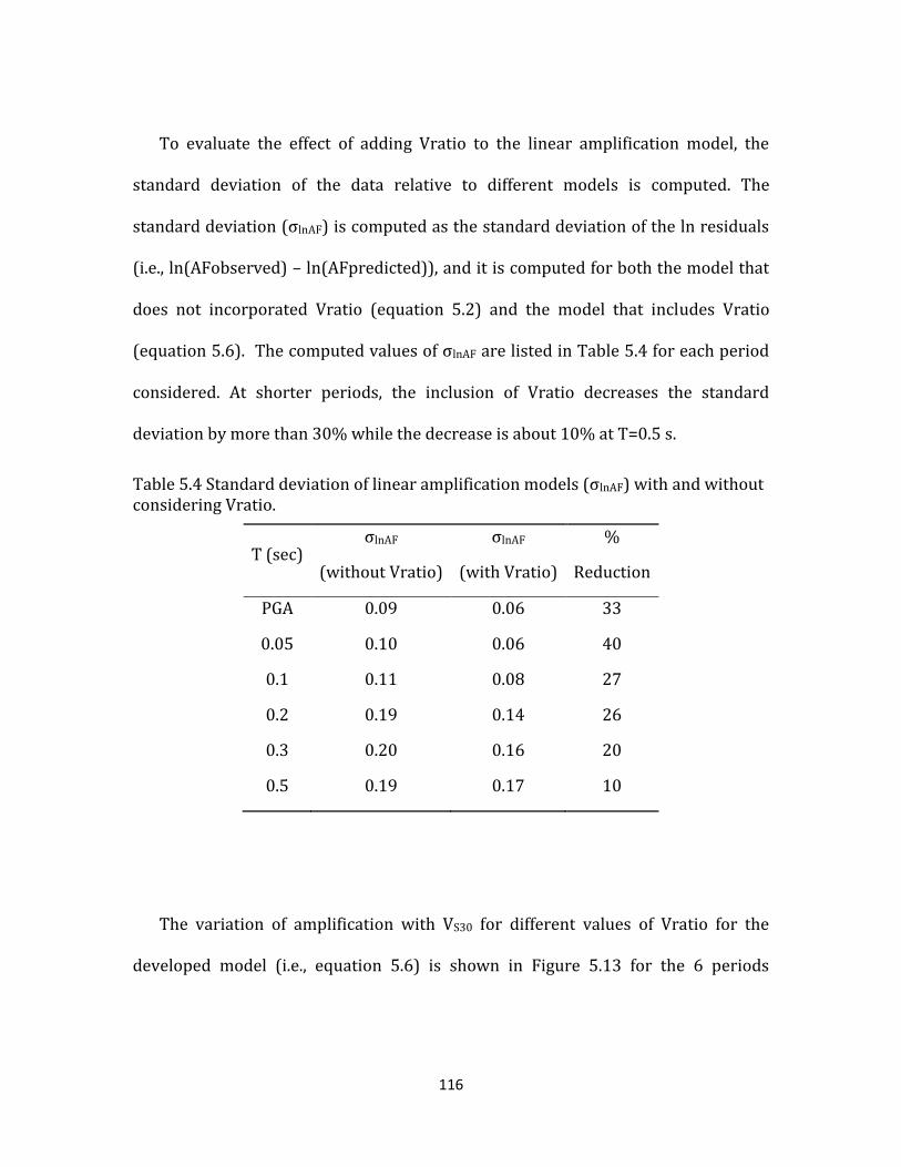
116
To evaluate the effect of adding Vratio to the linear amplification model, the
standard deviation of the data relative to different models is computed. The
standard deviation (σlnAF) is computed as the standard deviation of the ln residuals
(i.e., ln(AFobserved) – ln(AFpredicted)), and it is computed for both the model that
does not incorporated Vratio (equation 5.2) and the model that includes Vratio
(equation 5.6). The computed values of σlnAF are listed in Table 5.4 for each period
considered. At shorter periods, the inclusion of Vratio decreases the standard
deviation by more than 30% while the decrease is about 10% at T=0.5 s.
Table 5.4 Standard deviation of linear amplification models (σlnAF) with and without considering Vratio.
T (sec) σlnAF
(without Vratio)
σlnAF
(with Vratio)
%
Reduction
PGA 0.09 0.06 33
0.05 0.10 0.06 40
0.1 0.11 0.08 27
0.2 0.19 0.14 26
0.3 0.20 0.16 20
0.5 0.19 0.17 10
The variation of amplification with VS30 for different values of Vratio for the
developed model (i.e., equation 5.6) is shown in Figure 5.13 for the 6 periods

117
considered. The curves show how amplification is larger for larger values of Vratio,
and this effect is larger at smaller values of VS30.
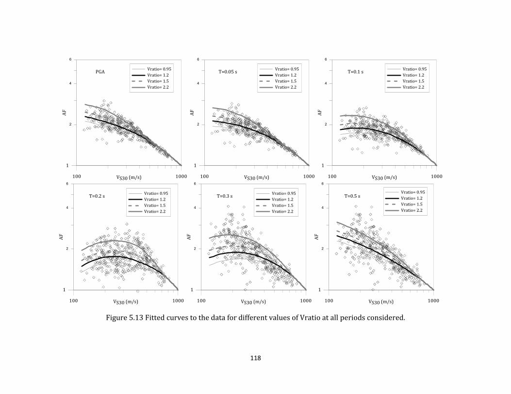
118
Figure 5.13 Fitted curves to the data for different values of Vratio at all periods considered.

119
5.4 Influence of Z1.0 on Amplification for Long
Periods
As discussed in the previous sections, a linear trend between ln(AF) and
ln(VS30/Vref) best fits the amplification data for periods greater than or equal to 0.5 s.
It is also shown that there is not a strong dependence of AF on Vratio for these
periods. Amplification at long periods is controlled predominantly by the depth of
soil, such that Z1.0 is an important parameter to include in the amplification model.
To consider the appropriate functional form for the amplification model that
includes Z1.0, the amplification data are separated into 4 bins of Z1.0 and AF is plotted
versus VS30/Vref for each bin. Figure 5.14 plots AF versus VS30/Vref for a spectral
period of 1.0 s. The slope of the linear fit of AF versus VS30 varies for different bins of
Z1.0 and generally increases with increasing Z1.0. This result indicates that the slope
of the linear fit is Z1.0 dependent. Figures 5.15, 5.16, and 5.17 show AF versus
VS30/Vref for the other long periods, and the same Z1.0 trends are observed at the
other periods.
A model for this relationship has been proposed by Kottke (2011), as presented
in Chapter 2, and is adopted in this study. This model is described as:
(5.7)

120
where
(5.8)
Z* is the depth (in meters) above which Z1.0 no longer influences the amplification
and a1 is the slope of the ln(AF) versus ln(VS30/Vref) relationship. In the model
proposed by Kottke (2011), Z* is defined as a function of frequency and b is constant
at all periods. In this study, Z* and b are estimated using the maximum likelihood
regression method for each period.
The parameters a1, Z*, and b are computed via a maximum likelihood regression
for the four long periods, and the values are listed in Table 5.5 along with the
standard deviation of model with and without considering Z1.0 effect. Small values of
Z* at periods of 1.0 and 2.0 s indicate that a smaller range of depth to bedrock
influences amplification at these periods. The reason that larger values of Z1.0 do not
influence amplification at T = 1.0 s and 2.0 s is because these larger values of Z1.0
generate amplification at much longer periods. The larger Z* values for periods of
5.0 and 10 s indicates that all values of Z1.0 influence amplification at these periods.
Figure 5.18 shows the variation of with Z1.0 for each long period. At T=1.0 s,
approaches 1 for Z1.0 greater than 100 m. While for T=10.0 s, does not reach 1.0
until Z1.0 is equal to 1000 m.
The variation of amplification with VS30 for different values of Z1.0 for the
developed model in equations (5.7) and (5.8) is shown in Figure 5.19 for the 4
periods considered. Relationships are shown for four values of Z1.0 that represent

121
the range in the data. The influence of Z1.0 at T=1.0 s is not significant different
because the derived value of Z* is relatively small. The influence of different values
of Z1.0 is more readily apparent in the data for periods of 5.0 and 10.0 s.
Nonetheless, the reduction in lnAF when Z1.0 is included is relatively modest (Table
5.5).
Table 5.5 Coefficients of the linear amplification model – Equation (5.7).
T(sec) a1 Z* (m) b σlnAF
(without Z1.0)
σlnAF
(with Z1.0)
1.0 -0.63 121 0.70 0.20 0.20
2.0 -0.75 292 0.71 0.19 0.17
5.0 -0.63 490 1.16 0.18 0.16
10.0 -0.44 1000 0.76 0.06 0.05

122
Figure 5.14 AF vesus VS30/Vref for 4 different bins of Z 1.0 at T=1.0 s.
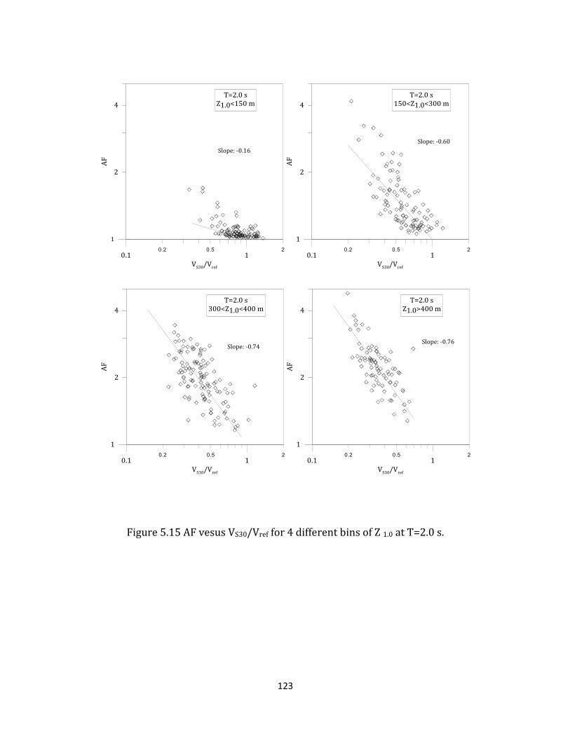
123
Figure 5.15 AF vesus VS30/Vref for 4 different bins of Z 1.0 at T=2.0 s.
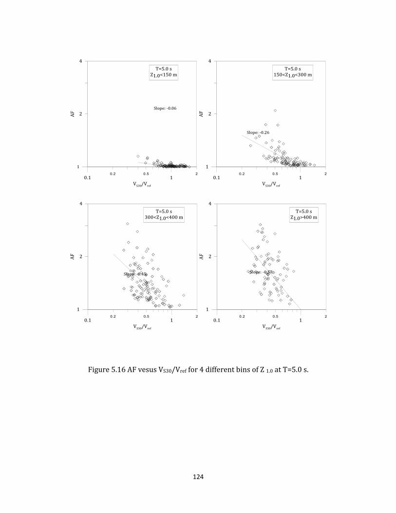
124
Figure 5.16 AF vesus VS30/Vref for 4 different bins of Z 1.0 at T=5.0 s.

125
Figure 5.17 AF vesus VS30/Vref for 4 different bins of Z 1.0 at T=10.0 s.

126
Figure 5.18 Variation of with Z1.0 for different long periods.

127
100 1000VS30 (m/s)
1
2
4
6
AF
Z1.0 = 80 m
Z1.0 = 230 m
Z1.0 = 350 m
Z1.0 = 450 m
T=1.0 s
Figure 5.19 Fitted curves to the data for different values of Z1.0 at all periods considered.

128
5.5 Summary
In this chapter, the linear component of the soil amplification models is developed.
At short periods, the relationship between AF and normalized VS30 (i.e., VS30/Vref) is
modified to a polynomial function. It is shown that the polynomial form improves
the fattiness of the model to the data. At short periods (T<1.0 s) which Vratio
influences the site amplification a term added to the linear component to
incorporates the effect of Vratio.
At longer periods (T≥ . s), it is shown that the linear relationship between AF
and the normalize VS30 fits the data the best. It is also identified the slope of this
linear relationship is Z1.0 dependent and the effect of Z1.0 at long periods are
considered in the developed linear component of the site amplification model at
long periods.
129
Chapter 6
Models for Nonlinear Site
Amplification
6.1 Introduction
As discussed in the previous chapters, the functional form of empirical site
amplification models includes two components; a linear elastic component and a
nonlinear component. The model for site amplification under linear-elastic
conditions is defined in Chapter 5 and the nonlinear component (NL) will be
discussed here. A functional form for shorter periods that includes the effects of
VS30 and Vratio will be presented, and a functional form for longer periods will be
presented that includes VS30 and Sa,rock.

130
6.2 VS30 Scaling for Nonlinear Models
The nonlinear component of the soil amplification model includes the effects of soil
nonlinearity at high intensity shaking, such that the amplification changes with
increasing input shaking intensity. The nonlinear effect can be modeled using a
functional form represented by:
(6.1)
where Sa,rock is the spectral acceleration for rock conditions at the spectral period of
interest, and b1 and c are regression coefficients. This functional form was used by
Chiou and Youngs(2008) in their NGA model.
It is helpful to consider how parameters b1 and c control the variation of AF with
shaking intensity (i.e., Sa,rock). Coefficient c essentially represents the Sa,rock level in
the middle of transition from linear behavior (i.e., where AF does not vary with
Sa,rock) to nonlinear behavior (i.e., where AF does vary with Sa,rock ). Coefficient b1
represents the degree of nonlinearity in terms of the logarithmic change in AF with a
logarithmic increase in the level of shaking .Generally, b1 is negative such that an
increase in Sa,rock results in a decrease in AF. A more negative value of b1 indicates a
stronger reduction in AF with Sa,rock (i.e. more nonlinearity), and as b1 approaches
zero the site amplification approaches the linear elastic condition. The degree of
nonlinearity is a function of the stiffness of the site; with softer sites experiencing
more nonlinearity. Therefore, b1 is a function of VS30.

131
Figure 6.1 shows AF versus Sa,rock as predicted by the Chiou and Youngs (2008)
NGA model at periods of PGA, 0.2, and 0.5 s and for 3 different VS30 values (150 m/s,
300 m/s and 500 m/s). Also shown are the locations of coefficient c for each period
(c is not taken VS30 dependent in the Chiou and Youngs (2008) model) and a
representative slope (b1) at larger Sa,rock . At each of the spectral periods,
nonlinearity is stronger at smaller values of VS30. At large values of VS30 (e.g.,
VS30=500m/s in Figure 6.1), the reduction of AF with increasing Sa,rock is insignificant
which indicates the more linear behavior of stiff sites. The coefficient c, which is the
shaking level transitioning from linear to nonlinear behavior, is close to 0.1 g at PGA
and 0.5 s, while it is higher (0.25 g) at a spectral period of 0.2 s.
To investigate the dependency of AF on Sa,rock and the factors that influence this
relationship, the computed AF values for the randomized site profiles subjected to
10 different input intensities are considered. Amplifications of the soil profiles at
short and long periods are considered separately in the next sections.

132
Figure 6.1 Amplification versus Sa,rock from the Chiou and Youngs NGA model (2008).

133
6.3 Nonlinear Site Amplification at Short Periods
Building upon previous work, the nonlinear AF model will be developed from
equation (6.1). The dependence of the slope b1 on VS30 is investigated by separating
the AF data into the same eight VS30 bins used in Chapter 5 (VS30<150 m/s,
150m/s<VS30<200 m/s, 200 m/s <VS30<250m/s, 250 m/s <VS30<300 m/s, 300 m/s
<VS30<350 m/s, 350 m/s <VS30<450 m/s, 450 m/s <VS30<550 m/s, and 550 m/s
<VS30<750 m/s). Figure 6.2 shows plots of AF versus Sa,rock for PGA for the eight bins
of VS30. At the smaller VS30 values amplification almost immediately starts to
decrease as Sa,rock increases from 0.01g. At larger VS30 (i.e. greater than about 300
m/s) AF remains relatively constant at Sa,rock level less than about 0.1g but then
decreases as Sa,rock increases beyond 0.1g. At the largest VS30 values AF does not vary
significantly over the Sa,rock values analyzed.
To identify the variation of b1 with VS30, a linear relationship is fit between the
logarithm of AF in each VS30 bin and the logarithm of Sa,rock, using only AF data from
Sa,rock >0.1 g in each bin. Only the data with Sa,rock larger than 0.1g is considered
because b1 represents the slope at larger input intensities. The slope of the linear
relationship (b1) is shown in Figure 6.2 and varies across the VS30 bins, with larger
VS30 values displaying smaller slopes. For T=0.2 s and 0.5 s (Figures 6.3 and 6.4,
respectively) a similar trend is observed with the slope decreasing with increasing
VS30. Figure 6.5 plots the derived values of b1 versus the median VS30 of each bin for
periods of PGA, 0.2, and 0.5 s. The data for all 3 periods show b1 as approximately

134
constant at smaller VS30 and then decreasing towards zero as VS30 increases. Above
some value of VS30, b1 tends to remains constant.
Using the trends in Figure 6.5, an expression that describes the slope b1 as a
function of VS30 is developed. This expression models b1 as decreasing log-linearly
between VS30 values of V1 and V2, and remaining constant outside of these values.
The VS30 below which b1 stays constant is V1 and the value above which b1 stays
constant is V2. bo1 and bo2 are the values of the slope for VS30 less than V1 and greater
than V2 , respectively. The resulting expression is given by:
(6.2)
V1, V2, bo1, and bo2 are regression coefficients that are period dependent. This
expression will be incorporated into the final form of the nonlinear amplification
model.

135
0.01 0.1 1 10
Sa,rock
0.01
0.1
1
10
AF
PGAVS30<150 m/s
Slope : -0.52
0.01 0.1 1 10
Sa,rock
0.01
0.1
1
10
AF
PGA150<VS30<200 m/s
Slope : -0.51
0.01 0.1 1 10
Sa,rock
0.01
0.1
1
10
AF
PGA200<VS30<250 m/s
Slope : -0.52
0.01 0.1 1 10
Sa,rock
0.01
0.1
1
10
AF
PGA250<VS30<300 m/s
Slope : -0.48
0.01 0.1 1 10
Sa,rock
0.01
0.1
1
10
AF
PGA300<VS30<350 m/s
Slope : -0.43
0.01 0.1 1 10
Sa,rock
0.01
0.1
1
10
AF
PGA350<VS30<450 m/s
Slope : -0.32
0.01 0.1 1 10
Sa,rock
0.01
0.1
1
10
AF
PGA450<VS30<550 m/s
Slope : -0.22
0.01 0.1 1 10
Sa,rock
0.01
0.1
1
10
AF
PGA550<VS30<750 m/s
Slope : -0.16
Figure 6.2 Amplification versus Sa,rock for different VS30 bins at PGA.
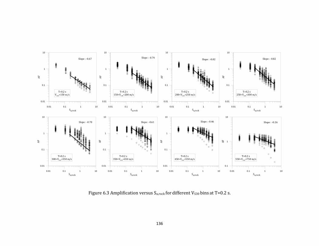
136
0.01 0.1 1 10
Sa,rock
0.01
0.1
1
10
AF
T=0.2 sVS30<150 m/s
Slope : -0.67
0.01 0.1 1 10
Sa,rock
0.01
0.1
1
10
AF
T=0.2 s150<VS 30<200 m/s
Slope : -0.74
0.01 0.1 1 10
Sa,rock
0.01
0.1
1
10
AF
T=0.2 s200<VS30<250 m/s
Slope : -0.82
0.01 0.1 1 10
Sa,rock
0.01
0.1
1
10
AF
T=0.2 s250<VS30<300 m/s
Slope : -0.82
0.01 0.1 1 10
Sa,rock
0.01
0.1
1
10
AF
T=0.2 s300<VS30<350 m/s
Slope : -0.78
0.01 0.1 1 10
Sa,rock
0.01
0.1
1
10
AF
T=0.2 s350<VS30<450 m/s
Slope : -0.61
0.01 0.1 1 10
Sa,rock
0.01
0.1
1
10
AF
T=0.2 s450<VS30<550 m/s
Slope : -0.46
0.01 0.1 1 10
Sa,rock
0.1
1
10
AF
T=0.2 s550<VS30<750 m/s
Slope : -0.26
Figure 6.3 Amplification versus Sa,rock for different VS30 bins at T=0.2 s.

137
0.01 0.1 1 10
Sa,rock
0.01
0.1
1
10
AF
T=0.5 sVS30<150 m/s
Slope : -0.88
0.01 0.1 1 10
Sa,rock
0.01
0.1
1
10
AF
T=0.5 s150<VS 30<200 m/s
Slope : -0.86
0.01 0.1 1 10
Sa,rock
0.01
0.1
1
10
AF
T=0.5 s200<VS30<250 m/s
Slope : -0.83
0.01 0.1 1 10
Sa,rock
0.01
0.1
1
10
AF
T=0.5 s250<VS30<300 m/s
Slope : -0.77
0.01 0.1 1 10
Sa,rock
0.1
1
10
AF
T=0.5 s300<VS30<350 m/s
Slope : -0.56
0.01 0.1 1 10
Sa,rock
0.01
0.1
1
10
AF
T=0.5 s350<VS30<450 m/s
Slope : -0.28
0.01 0.1 1 10
Sa,rock
0.1
1
10
AF
T=0.5 s450<VS30<550 m/s
Slope : -0.09
0.01 0.1 1 10
Sa,rock
0.1
1
10
AF
T=0.5 s550<VS30<750 m/s
Slope : -0.07
Figure 6.4 Amplification versus Sa,rock for different VS30 bins at T=0.5 s.
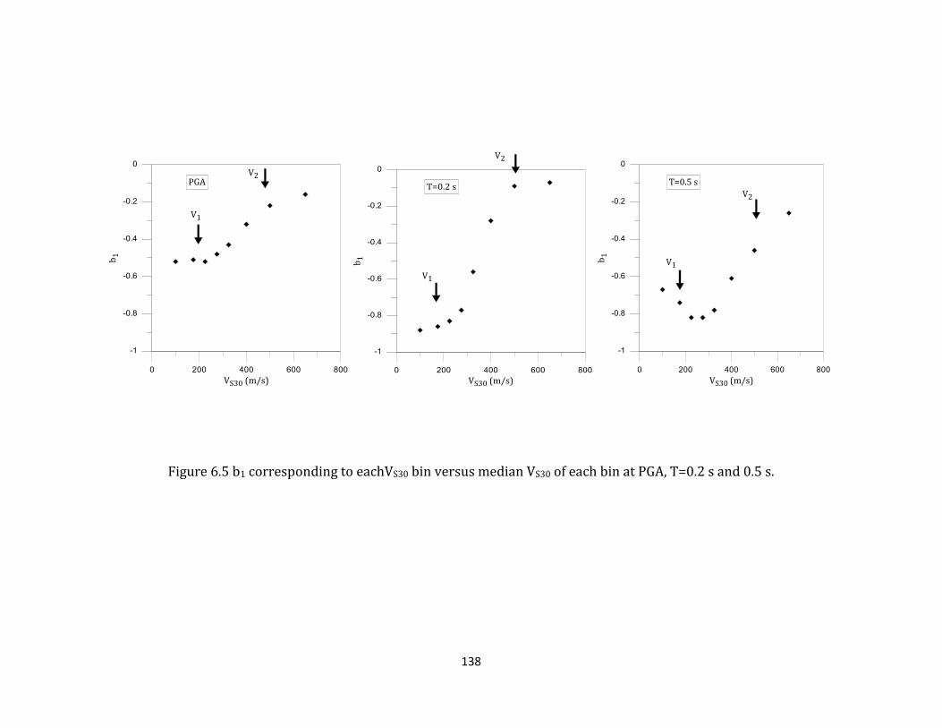
138
Figure 6.5 b1 corresponding to eachVS30 bin versus median VS30 of each bin at PGA, T=0.2 s and 0.5 s.
139
6.3.1 Influence of Vratio on Nonlinear Site Response
It was shown in Chapter 5 that Vratio influences the linear-elastic amplification of
soil sites at shorter periods. Including Vratio into the linear-elastic model reduced
the standard deviation by 10 to 30%. The Vratio effect modeled in the linear elastic
amplification model will be present at larger intensities, but Vratio may also
influence the nonlinear amplification. The AF data in Figures 6.2 through 6.4 clearly
show that the scatter in the AF data increases as input intensity increases. Based on
the observations at small input intensities, Vratio is likely influencing the computed
values of AF at large input intensities.
To investigate the influence of Vratio on the nonlinear component of the site
amplification model, AF is plotted versus the normalized Vratio (Vratio/1.4) for
each bin of VS30 and input intensity. A linear relationship is fit to the ln(AF) versus
ln(Vratio/1.4) for each Sa,rock to identify if the slope of this relationship (i.e.,
regression parameter a3 from Chapter 5) is Sa,rock dependent. Figures 6.6 through 6.8
show plots of PGA amplification versus Vratio/1.4 for VS30 bins of <150 m/s, 250-
350 m/s and 550-750 m/s, respectively. The slope of the log-linear fit for each of the
VS30 bins generally increases with Sa,rock. The slope, which indicates how strongly
Vratio affects AF for a given VS30, can increase by more than a factor of two as Sa,rock
increases from 0.01g to 0.9g. For the larger VS30 values (Figure 6.8), the slope
increases from 0.0 (i.e., no Vratio effect) at Sa,rock=0.01g to 0.4 at Sa,rock=0.9g.

140
The slope of the linear fit between ln(AF) and ln(Vratio/1.4), which represents
parameter a3 in the linear-elastic model of Chapter 5 is plotted versus normalized -
Sa,rock (i.e., Sa,rock/Sa,rock-min, where Sa,rock-min is the smallest input rock intensity
considered) in Figure 6.9 for all eight VS30 bins. Chapter 5 demonstrated that a3 is
VS30 dependent; Figure 6.9 allows us to investigate whether the increase in a3 with
Sa,rock is also VS30 dependent. The data in Figure 6.9 show that a3 increases linearly
with ln(Sa,rock/Sa,rock-min) for all VS30 bins at PGA.

141
Figure 6.6 Amplification versus normalized Vratio for VS30<150 m/s at PGA.

142
Figure 6.7 Amplification versus normalized Vratio for 250<VS30<300 m/s at PGA.

143
Figure 6.8 Amplification versus normalized Vratio for 550<VS30<750 m/s at PGA.

144
Figure 6.9 The slope of linear fit between ln(AF) and ln(Vratio/1.4) versus Sa,rock /Sa,rock-min at PGA.

145
The linear trend between a3 and ln (Sa,rock/Sa,rock-min) is quite strong, and the slope of
that relationship varies between 0.05 and 0.15, with most of the values between
0.07 and 0.09. The computed slopes are plotted versus VS30 in Figure 6.10. The
variation of the slope with VS30 is not systematic, and therefore, the slope is
considered VS30 independent.
Generally, the trends shown for PGA are similar for other short periods (i.e., ≤ .5
s), Figure 6.11 plots the slope of the a3 versus ln (Sa,rock/Sa,rock-min) relationship
versus VS30 for these other periods. Again, the slope varies with VS30 but not in a
systematic manner. Therefore, the slope is modeled as VS30-independent for all of
the short periods.
Figure 6.10 The variation of the slope of the linear fit between a3 and ln(Sa,rock /Sa,rock-min ) with VS30 at PGA.

146
Figure 6.11 The variation of the slope of the linear fit between a3 and ln(Sa,rock /Sa,rock-min ) with VS30 at T=0.05,0.1, 0.2,0.3 and 0.5 s.
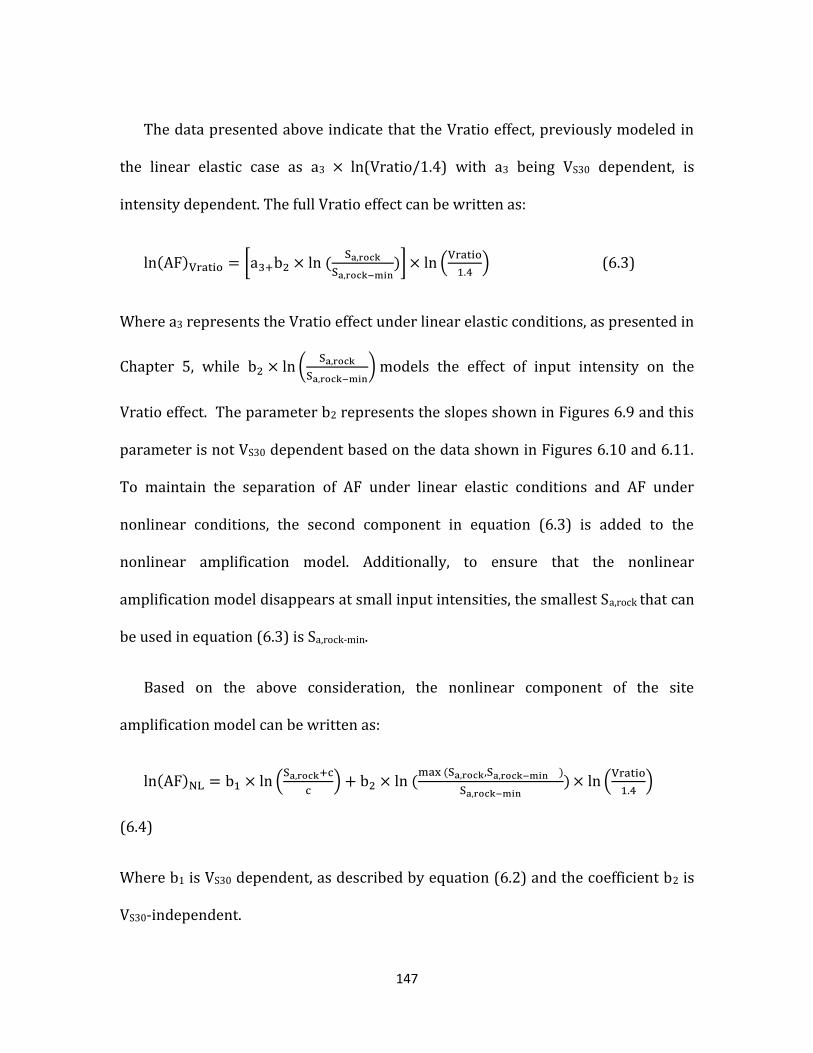
147
The data presented above indicate that the Vratio effect, previously modeled in
the linear elastic case as a3 ln(Vratio/1.4) with a3 being VS30 dependent, is
intensity dependent. The full Vratio effect can be written as:
(6.3)
Where a3 represents the Vratio effect under linear elastic conditions, as presented in
Chapter 5, while
models the effect of input intensity on the
Vratio effect. The parameter b2 represents the slopes shown in Figures 6.9 and this
parameter is not VS30 dependent based on the data shown in Figures 6.10 and 6.11.
To maintain the separation of AF under linear elastic conditions and AF under
nonlinear conditions, the second component in equation (6.3) is added to the
nonlinear amplification model. Additionally, to ensure that the nonlinear
amplification model disappears at small input intensities, the smallest Sa,rock that can
be used in equation (6.3) is Sa,rock-min.
Based on the above consideration, the nonlinear component of the site
amplification model can be written as:
(6.4)
Where b1 is VS30 dependent, as described by equation (6.2) and the coefficient b2 is
VS30-independent.

148
6.4 Nonlinear Site Amplification at Long Periods
To investigate the dependency of amplification on input intensity at long periods, AF
is plotted versus Sa,rock for bins of VS30 at the four long periods considered. Figures
6.12 and 6.13 show AF versus Sa,rock for two select representative periods: T=1.0s
and 5.0 s, respectively. At T= 1.0 s, AF decreases with increasing input intensity
(Sa,rock) for smaller VS30 but the AF remains constant or slightly increases for larger
VS30 (i.e., greater than about 350 m/s in Figure 6.12). At T=5.0 s (Figure 6.13),
amplification generally increases as Sa,rock increases for smaller VS30, indicating that
the b1 slope may be positive at long periods. At larger values of VS30, the
amplification becomes insensitive to input intensity (slope ~ 0.0) similar to the
results for T=1.0 s. A positive value of b1 is technically justified for T=5.0 s, because
most sites have natural periods shorter than 5.0 s and the soil nonlinearity induced
by large input intensities will cause period lengthening towards 5.0 s. This
lengthening will cause an increase in amplification with increasing input intensity at
this period. Sites with larger VS30 tend to have natural periods much shorter than 5.0
s and they strain less as Sa,rock increases, making the effect of period lengthening
minimal.
The slope of the ln(AF)-ln(Sa,rock) relationship at larger values of Sa,rock (i.e., b1)
are computed for each VS30 bin and are shown in Figures 6.12 and 6.13. Figure 6.14
plots the derived values of b1 versus the median VS30 of each bin for periods of 1.0 s
and 5.0 s. Figure 6.14 shows that b1 is constant at smaller VS30, it varies linearly with

149
increasing VS30, and then becomes constant again at larger VS30. For T=1.0 s, b1 is
equal to -0.8 at smaller VS30 and approaches 0.0 at VS30 greater than about 400 m/s.
For T=5.0 s, b1 is about 0.2 for smaller VS30 and approaches 0.0 at VS30 greater than
about 500 m/s. A positive value of b1 indicates that AF increases with increasing
Sa,rock, and positive values are observed for periods greater than and equal to 2.0 s.
Based on the data presented in Figure 6.14, the same functional form that is used
at short periods to describe the variation b1 with VS30 can be used at longer periods
(equation 6.2). This relationship defines regions of constant b1 at smaller and larger
VS30 values, and a linear relationship with ln(VS30) in between. The regression
parameters are the VS30 values above and below which b1 is a constant (V2 and V1),
and the b1 values above and below these values (bo2 and bo1).
In Chapter 5, it was shown that the site amplification at long periods is not
influenced by Vratio, but that it is influenced by Z1.0. Z1.0 is not affected by soil
nonlinearity and therefore is not affected by input intensity (i.e., Sa,rock). Combining
the linear and nonlinear components, the amplification model at long periods can be
expressed as:
(6.5)

150
where is a function of Z1.0 as defined by Equation (5.8) and b1 is a function of VS30
as defined by equation (6.2).

151
Figure 6.12 Amplification versus Sa,rock for different VS30 bins at T=1.0 s.
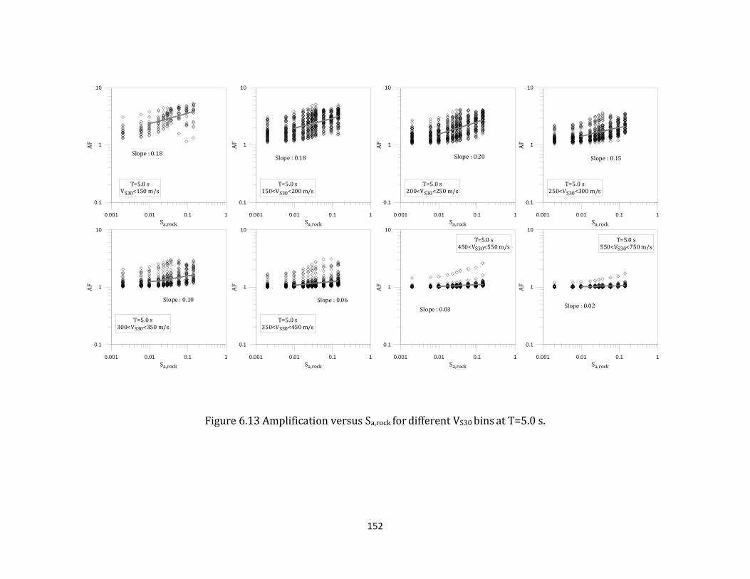
152
0.001 0.01 0.1 1
Sa,rock
0.1
1
10A
F
T=5.0 sVS30<150 m/s
Slope : 0.18
0.001 0.01 0.1 1
Sa,rock
0.1
1
10
AF
T=5.0 s150<VS30<200 m/s
Slope : 0.18
0.001 0.01 0.1 1
Sa,rock
0.1
1
10
AF
T=5.0 s200<VS30<250 m/s
Slope : 0.20
0.001 0.01 0.1 1
Sa,rock
0.1
1
10
AF
T=5.0 s250<VS30<300 m/s
Slope : 0.15
0.001 0.01 0.1 1
Sa,rock
0.1
1
10
AF
T=5.0 s300<VS30<350 m/s
Slope : 0.10
0.001 0.01 0.1 1
Sa,rock
0.1
1
10A
F
T=5.0 s350<VS30<450 m/s
Slope : 0.06
0.001 0.01 0.1 1
Sa,rock
0.1
1
10
AF
T=5.0 s450<VS30<550 m/s
Slope : 0.03
0.001 0.01 0.1 1
Sa,rock
0.1
1
10
AF
T=5.0 s550<VS30<750 m/s
Slope : 0.02
Figure 6.13 Amplification versus Sa,rock for different VS30 bins at T=5.0 s.

153
Figure 6.14 b1 corresponding to eachVS30 bin versus median VS30 of each bin at T=1.0 s and 5 s.

154
6.5 Summary
This chapter described the development of the nonlinear amplification model, which
describes the variation of site amplification with increases in input shaking intensity
(Sa,rock). Separate nonlinear models are developed for short and long periods. It
was shown that at short periods , the logarithm of amplification vary with the
logarithm of Sa,rock and this variation is VS30 dependent as softer sites show more
nonlinearity ( i.e., more reduction in amplification with increase of Sa,rock). The
influence of Vratio is also incorporated at the nonlinear component of the site
response model. The influence of Vratio on amplification is Sa,rock dependent but VS30
independent.
At longer periods, the same functional form for considering the variation of
amplification with input intensity at short periods is considered. However, at long
periods Vratio does not influence the site amplification.
155
Chapter 7
Final Site Amplification Model
7.1 Introduction
The linear and nonlinear components of the site amplification model presented in
Chapters 5 and 6 are combined in this chapter. Separate functional forms are fit to
the amplification data for short and long periods. To demonstrate the fit of the
developed model, the amplification data are plotted along with predictions from the
developed models. The calculated residuals from the developed functional forms
are plotted versus the independent variables in the site amplification model.

156
7.2 Combined Model for Short Periods
Combining the linear-elastic and nonlinear components of the amplification model
for short periods, the following model is proposed for the amplification factor for
spectral accelerations at short periods (T≤ .5 s):
(7.1a)
(7.1b)
This model is fit independently to each short period. The parameters a3 and b1
are VS30 dependent, and the VS30-dependencies are described by:
(7.2)
and
(7.3)

157
All other parameters are not a function of VS30.
The regression process is executed in three steps. Each step uses the maximum
likelihood method for regression. In the first step, the coefficients for the linear-
elastic component are estimated (i.e., a1, a2, a0, Va, Vb) using the AF data from the
lowest intensity input motions (i.e., PGArock=0.01g). These parameters are kept
fixed in subsequent steps. In the second step, the parameters for the nonlinear
model (bo1, bo2, V1, V2, and c) are estimated excluding the effect of Vratio (i.e., b2)
using the AF data for all input intensities. To ensure that the nonlinear component
of the model does not influence the computed amplification at small Sa,rock, a
minimum value of c was set to 0.1 g. If c=0.1 g, then the
term is equal to
0.095 for Sa,rock = 0.01 g. Thus, the nonlinear effect on the computed amplification
will be minimal. In the last and final step, all previously parameters are fixed and b2
(i.e., the Vratio effect in the nonlinear model) is computed. The final estimated
values of all coefficients for the 6 short periods studied here are listed in Table 7.1.

158
Table 7.1 Coefficients of the site amplification model for short periods–Equation (7.1).
T (sec) PGA 0.05 s 0.1 s 0.2s 0.3s 0.5s
a1 -0.69 -0.70 -0.76 -0.9 -0.89 -0.67
a2 -0.13 -0.15 -0.21 -0.32 -0.28 -0.10
a3 model
a0 0.34 0.38 0.38 0.44 0.57 0.39
Va (m/s) 176 130 110 414 100 100
Vb (m/s) 481 513 737 726 750 750
b1 model
bo1 -0.91 -1.26 -0.98 -1.21 -1.93 -2.60
bo2 -0.24 -0.21 -0.19 -0.16 -0.14 -0.11
V1 (m/s) 184 118 192 188 133 103
V2 (m/s) 454 581 583 557 530 447
c 0.1 0.1 0.1 0.21 0.37 0.4
b2 0.09 0.08 0.08 0.07 0.08 0.06
Vref (m/s) 1000 1000 1000 1000 1000 1000
Sa,rock-min (g) 0.01 0.01 0.02 0.03 0.03 0.03
Figure 7.1 shows the residuals (i.e., ln(data)-ln(predicted) plotted versus VS30,
Sa,rock, and Vratio for the amplification factors for PGA. The residuals indicate
overprediction in amplification (negative residuals) for smaller VS30 and a slight
overprediction over all VS30 (overall average residual equal to -0.07). There is no
systematic trend between the residuals and the various parameters. However the
variability in the residuals increases with the increase of Sa,rock. For all the other
considered short periods, the residual also do not show a systematic trend with any

159
of independent variables in the model. However, the average residual across these
other periods range from about -0.07 to +0.08.
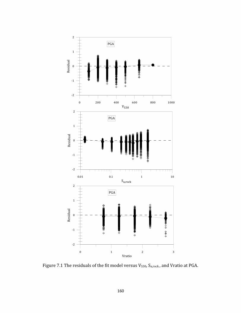
160
Figure 7.1 The residuals of the fit model versus VS30, Sa,rock , and Vratio at PGA.

161
It is difficult to fully evaluate the model looking at the overall residuals, therefore
AF predictions are plotted versus Sa,rock along with the AF data in the next several
figures. To demonstrate the effects of VS30 and Vratio on the AF predictions, the
predicted AF values are plotted versus Sa,rock for select VS30 bins and for a range of
Vratio values. As discussed previously, the range of Vratio values is slightly different
among the VS30 bins, but most of the values fall between 0.8 and 2.5. Considering
these ranges, AF predictions are shown for Vratio=0.8, 1.4, and 2.5 in Figures 7.2 to
7.7 for the 6 periods considered.
The predictions in Figures 7.2 through 7.7 are in general agreement with the
data. Additionally, sites with larger values of Vratio have larger amplification and
sites with smaller Vratio have smaller amplification. This effect helps explain some
of the scatter shown in the AF data. For each period, the effect of Vratio at low input
intensity (i.e., smallest Sa,rock) is strongest for the smaller values of VS30 and
essentially non-existent for larger VS30 (greater than about 350 m/s). However, the
input intensity effect modeled with Vratio results in Vratio becoming important for
larger VS30 at larger input intensities (note the predictions for VS30=450-550 m/s in
Figures 7.2 to 7.7).
While there is general agreement in Figures 7.2 through 7.7, there are some
areas of deviation. Note that at the smallest input intensity and the smallest VS30
values, the AF predictions tend to be smaller than observed for T 0.2 s. This result
is due to the parameter c being small (~ 0.1 g) relative to the smallest Sa,rock used in

162
this study (0.01 g) and the large, negative values of b1 for small VS30 sites. As a
result, the nonlinear component of the amplification model contributes to the AF
prediction even for Sa,rock ~ 0.01 g. This issue is not apparent at periods of 0.3 and
0.5 s because the parameter c is larger (Table 7.1). Another challenging area is
amplification for the larger VS30 values (450 to 550 m/s) at periods of 0.1 and 0.2 s.
The model tends to underpredict the amplification at moderate Sa,rock and
overpredict amplification at larger AF. This issue again appears to be due to c being
relatively small and the model for the VS30-dependence for b1.

163
Figure 7.2 AF versus Sa,rock and fitted curves to the data for different values of Vratio at PGA.

164
Figure 7.3 AF versus Sa,rock and fitted curves to the data for different values of Vratio at T=0.05 s.
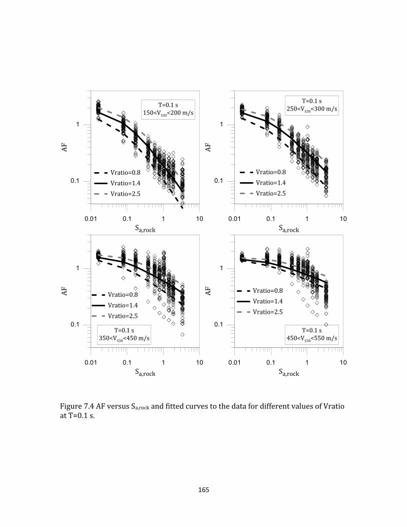
165
Figure 7.4 AF versus Sa,rock and fitted curves to the data for different values of Vratio at T=0.1 s.
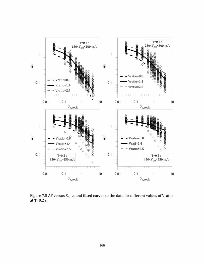
166
Figure 7.5 AF versus Sa,rock and fitted curves to the data for different values of Vratio at T=0.2 s.

167
Figure 7.6 AF versus Sa,rock and fitted curves to the data for different values of Vratio at T=0.3 s.

168
Figure 7.7 AF versus Sa,rock and fitted curves to the data for different values of Vratio at T=0.5 s.

169
To evaluate the effect of adding Vratio to the full amplification model, the
standard deviation of the residuals (i.e., ln(data)-ln(predicted)) for models with and
without including ratio is computed. The standard deviations (i.e., σlnAF) are listed
in Table 7.2 for each period. The standard deviation of the full model decreases
when including Vratio (in most cases from about 8% to 15%), however the level of
reduction is not as significant as it was for the linear model (Chapter 5). The modest
reduction in σlnAF may be influenced by the strength of ln(AF)-ln(Vratio)
relationship at larger input intensities. Considering the data shown in Figures 6.6-
6.8, the variability about the linear relationship increases with increasing intensity
indicating that the strength of the relationship decreases with increasing input
intensity. In addition to the standard deviation of the residuals, to compare two
models with and without Vartio,
is calculated at each period. is
defined as :
(7.4)
where is the sum of the squared residuals from model 1 (i.e. the
model that does not include Vratio) and is the sum of the squared
residuals from model 2 (i.e. the model that includes Vratio).The calculated
values for each period is given in Table 7.2. The values range from 0.08 to
0.33 indicating that Vratio model explains 8% to 33% of the variation within the
non-Vratio model At a spectral period of 0.2 s, the calculated reaches its
maximum value of 33%.
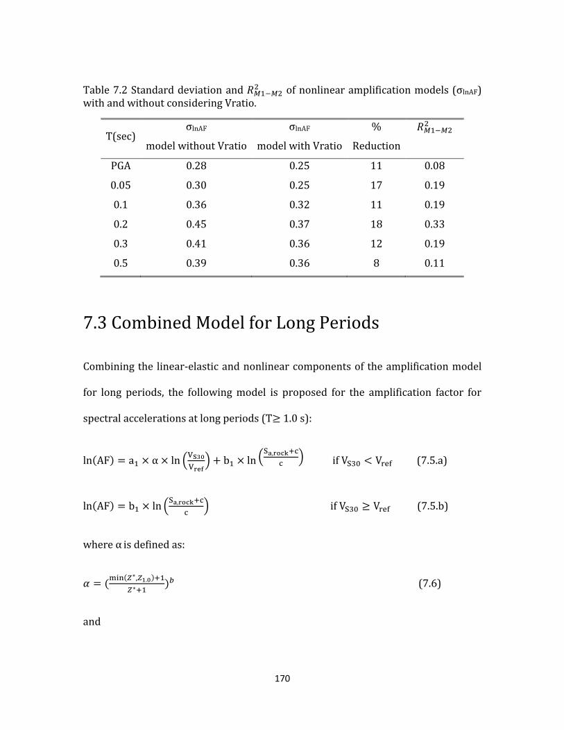
170
Table 7.2 Standard deviation and of nonlinear amplification models (σlnAF)
with and without considering Vratio.
T(sec) σlnAF
model without Vratio
σlnAF
model with Vratio
%
Reduction
PGA 0.28 0.25 11 0.08
0.05 0.30 0.25 17 0.19
0.1 0.36 0.32 11 0.19
0.2 0.45 0.37 18 0.33
0.3 0.41 0.36 12 0.19
0.5 0.39 0.36 8 0.11
7.3 Combined Model for Long Periods
Combining the linear-elastic and nonlinear components of the amplification model
for long periods, the following model is proposed for the amplification factor for
spectral accelerations at long periods (T 1.0 s):
(7.5.a)
(7.5.b)
where is defined as:
(7.6)
and
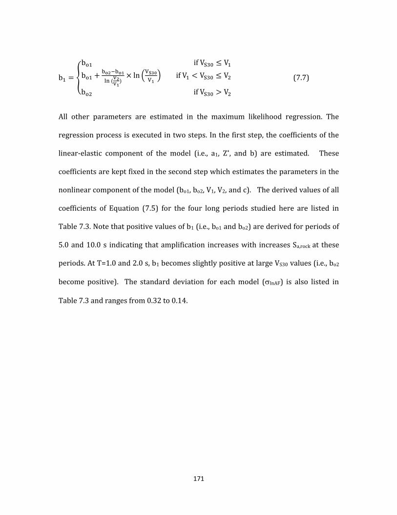
171
(7.7)
All other parameters are estimated in the maximum likelihood regression. The
regression process is executed in two steps. In the first step, the coefficients of the
linear-elastic component of the model (i.e., a1, Z*, and b) are estimated. These
coefficients are kept fixed in the second step which estimates the parameters in the
nonlinear component of the model (bo1, bo2, V1, V2, and c). The derived values of all
coefficients of Equation (7.5) for the four long periods studied here are listed in
Table 7.3. Note that positive values of b1 (i.e., bo1 and bo2) are derived for periods of
5.0 and 10.0 s indicating that amplification increases with increases Sa,rock at these
periods. At T=1.0 and 2.0 s, b1 becomes slightly positive at large VS30 values (i.e., bo2
become positive). The standard deviation for each model (lnAF) is also listed in
Table 7.3 and ranges from 0.32 to 0.14.

172
Table 7.3 Coefficients of the site amplification model for long periods –Equation (7.5).
T (sec) 1.0 2.0 5.0 10.0
a1 -0.62 -0.75 -0.63 -0.44
Z* (m) 121 292 490 1000
b 0.70 0.71 1.16 0.76
bo1 -1.6 -0.70 0.17 0.36
b02 0.06 0.10 0.02 0.04
V1 (m/s) 114 120 193 143
V1 (m/s) 387 380 470 390
c 0.2 0.15 0.005 0.005
Vref(m/s) 850 600 500 500
σlnAF 0.32 0.27 0.21 0.14
Figure 7.8 shows the residuals (i.e., ln(data)-ln(predicted) plotted versus VS30,
Sa,rock, and Z1.0 for spectral period of 1.0 s. The residuals do not show any systematic
trend with respect to VS30, Sa,rock, and Z1.0 . For all the other considered long periods,
the residuals do not show any systematic trend with any of independent variables in
the model.
To investigate how the proposed functional form at long periods (T ≥ . s) fits
the data, predictions of AF are plotted versus Sa,rock for three different values of Z1.0
in Figures 7. 9 to 7.12 for the four long periods considered in this study. The AF data

173
are also shown in these plots. As discussed before, there is a relationship between
VS30 of a site and its depth to the bedrock (i.e. Z1.0). Stiffer sites reach bedrock at
shallower depth. Based on the data shown in Chapter 4 for VS30<300 m/s, Z1.0 ranges
from about 100 to 600 m. Therefore, the predicted AF values are plotted for Z1.0 of
100, 300 and 600 m for VS30>300 m/s. For VS30 > 300 m/s, Z1.0 ranges from 20 to
400 m. For VS30 > 300 m/s, AF predictions are shown for Z1.0 of 20, 200, and 400 m.
As discussed in the previous chapter, the parameter incorporates the effect of
depth in the model and is equal to . for sites with Z1.0 greater than Z*. Therefore,
amplification for sites with Z1.0 > Z* is not influenced by Z1.0.
At a spectral period of 1.0 s (Figure 7.9), Z* is equal to 121 m such that most of
the curves shown do not show any Z1.0 effect. The curve with Z1.0 equal to 100 m for
VS30 < 300 m/s shows a very small effect and the curve for Z1.0 equal to 20 m for VS30
> 300 m/s shows a larger effect. However, few of the data have Z1.0 equal to 20 m.
Similar trends are observed at T=2.0 s, but with Z* equal to 292 m the Z1.0 effect is
more apparent. At longer periods (i.e., 5.0 and 10.0 s), Z* is much larger (490 and
1000 m respectively) such that a clear increase in amplification as depth to the
bedrock (Z1.0) increases is observed for VS30<300 m/s. For larger VS30, the VS30
approaches Vref (i.e., Vref = 500 m/s for these periods, and AF= 1.0 for VS30 > Vref)
such that the Z1.0 effect is not significant.
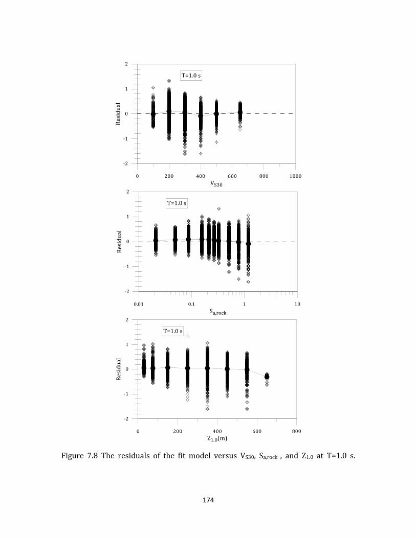
174
Figure 7.8 The residuals of the fit model versus VS30, Sa,rock , and Z1.0 at T=1.0 s.

175
Figure 7.9 Fitted curves to the data for different values of Z1.0 for each bin of VS30 at T=1.0 s.

176
Figure 7.10 Fitted curves to the data for different values of Z1.0 for each bin of VS30 at T=2.0 s.

177
Figure 7.11 Fitted curves to the data for different values of Z1.0 for each bin of VS30 at T=5.0 s.

178
Figure 7.12 Fitted curves to the data for different values of Z1.0 for each bin of VS30 at T=10.0 s.

179
7.4 Summary
In this chapter, the linear and nonlinear components of the developed site
amplification model are combined. Separate site response models are presented for
short and long periods

180
Chapter 8
Amplification Prediction
8.1 Introduction
To compare the proposed model in this study to the site amplification models
already used in ground motion prediction equations, several scenario events (i.e.
input motion intensities) and soil profiles are considered. The responses predicted
by the model developed in this study are compared to predictions from the NGA
models. The influence of Vratio on the predicted amplification is also discussed.
The limitation of the developed model and the range of input motion intensities
over which the model can be accurately used are addressed.
8.2 Scenario Events
Two sites with different VS30 values and three input motion intensities are
considered to compare the developed model and the NGA models. To show the
influence of Vratio on the prediction of amplification, the amplification for each site
is predicted for three values of Vratio (i.e., Vratio=0.85, 1.4, and 2.3) and their
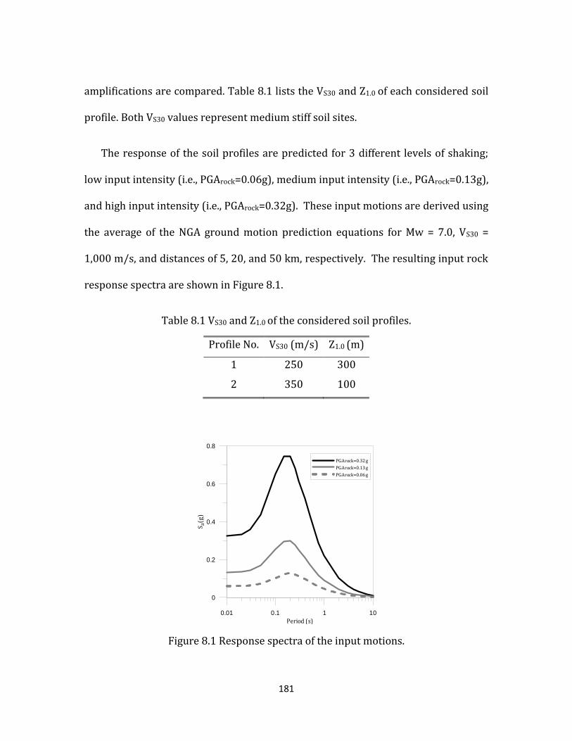
181
amplifications are compared. Table 8.1 lists the VS30 and Z1.0 of each considered soil
profile. Both VS30 values represent medium stiff soil sites.
The response of the soil profiles are predicted for 3 different levels of shaking;
low input intensity (i.e., PGArock=0.06g), medium input intensity (i.e., PGArock=0.13g),
and high input intensity (i.e., PGArock=0.32g). These input motions are derived using
the average of the NGA ground motion prediction equations for Mw = 7.0, VS30 =
1,000 m/s, and distances of 5, 20, and 50 km, respectively. The resulting input rock
response spectra are shown in Figure 8.1.
Table 8.1 VS30 and Z1.0 of the considered soil profiles.
Profile No. VS30 (m/s) Z1.0 (m)
1 250 300
2 350 100
0.01 0.1 1 10
Period (s)
0
0.2
0.4
0.6
0.8
Sa(g
)
PGArock=0.32 g
PGArock=0.13 g
PGArock=0.06 g
Figure 8.1 Response spectra of the input motions.

182
8.3 Site Amplification Predicted by NGA Models
Four of the NGA models contain site amplification models that model soil
amplification as a continuous function of VS30. The AF predicted by the NGA models
varies between the models. Figure 8.2 shows the predicted AF versus period for
each model for a site with VS30=250 m/s and the three input motion scenarios (i.e.,
PGArock=0.06g, 0.13g, and 0.32g). The average predicted AF across the four models is
also shown in Figure 8.2. For the smallest PGArock, the four models predict similar
levels of amplification that range from about 1.5 at short periods to over 3.0 at long
periods. The Campbell and Bozorgnia (2008) prediction is noticeably smaller at
short periods and the Abrahamson and Silva (2008) prediction is noticeably smaller
at long periods. As the input intensity increases, the predicted AF values at short
periods decrease while those at long periods remain the same because soil
nonlinearity is not modeled strongly at long periods in the NGA models. Across all
input intensities, the Campbell and Bozorgnia (2008) prediction is smaller at short
periods and the Abrahamson and Silva (2008) prediction is smaller at long periods.
Figure 8.3 shows the predicted AF versus period for each NGA model for a site with
VS30=350 m/s and the same three input motions scenarios. The trends observed for
the site with VS30= 250 m/s in Figure 8.2 are observed for this site as well. Across all
input intensities, the Campbell and Bozorgnia (2008) prediction is smaller at short
periods and the Abrahamson and Silva (2008) prediction is smaller at long periods.

183
0.01 0.1 1 10
Period (s)
0.1
1
10
AF
A&S (2008)
B&A (2008)
C&B (2008)
C&Y (2008)
Average
PGArock=0.06g
VS30=250 m/s
0.01 0.1 1 10
Period (s)
0.1
1
10
AF
A&S (2008)
B&A (2008)
C&B (2008)
C&Y (2008)
Average
PGArock=0.13g
VS30=250 m/s
0.01 0.1 1 10
Period (s)
0.1
1
10
AF
A&S (2008)
B&A (2008)
C&B (2008)
C&Y (2008)
Average
PGArock=0.32g
VS30=250 m/s
Figure 8.2 Predicted AF by different NGA models for a site with VS30=250 m/s subjected to three input intensities.

184
0.01 0.1 1 10
Period (s)
0.1
1
10
AF
A&S (2008)
B&A (2008)
C&B (2008)
C&Y (2008)
Average
PGArock=0.06g
VS30=350 m/s
0.01 0.1 1 10
Period (s)
0.1
1
10
AF
A&S (2008)
B&A (2008)
C&B (2008)
C&Y (2008)
Average
PGAroc k=0.13g
VS30=350 m/s
0.01 0.1 1 10
Period (s)
0.1
1
10
AF
A&S (2008)
B&A (2008)
C&B (2008)
C&Y (2008)
Average
PGArock=0.32g
VS30=350 m/s
Figure 8.3 Predicted AF by different NGA models for a site with VS30=350 m/s subjected to three input intensities.

185
8.4 Site Amplification Predicted by the Developed
Model
The AF values predicted by the developed site amplification model for the scenarios
discussed and Vratio equal to 0.85, 1.4, and 2.3 are shown in Figure 8.4. The
different values of Vratio influence amplification at periods less than 1.0 s, and the
difference can be significant at high input intensities. Here, an increase in Vratio
from 0.85 to 2.3 can increase the amplification by as much as a factor of 2.0.
Applying the amplification factors from Figure 8.4 to the rock response spectra from
Figure 8.1 result in the soil surface response spectra in Figure 8.5. In all cases, the
response of the sites shifts the spectrum to longer periods with the peaks occurring
at 0.3 to 0.4 s rather than at 0.2 s. The influence of different values of Vratio is
readily apparent, with the PGA and Sa,max significantly larger for larger Vratio.
Figure 8.6 compares the average AF predicted by the NGA models (shown in
Figures 8.2 and 8.3) with those predicted by the developed model for the six
scenarios. It is clear that the AF values predicted by this study are almost all smaller
than those predicted by the NGA models. The difference is most significant for VS30
= 250 m/s and PGArock = 0.32 g.
The differences are most likely due to the different datasets upon which the
models were developed. The VS30 scaling for the linear elastic component of the
NGA models was constrained based on ground motion recordings. Only one-third of

186
the NGA sites have measured values of VS30 and the others sites have inferred
values; this uncertainty introduces uncertainty in the VS30 scaling of the NGA
models. Additionally, the NGA recordings may include effects beyond one-
dimensional site amplification and these effects are not modeled in the site response
simulations used in this study. The nonlinear VS30 scaling in the NGA models is
typically constrained by some form of site response simulations (e.g., Walling et al.
2008), yet these simulations mainly focused on VS30 values greater than 300 m/s. At
long periods, the soil depth scaling of several of the NGA models was constrained
using three-dimensional basin simulations (e.g., Day et al 2008), and these
simulations will certainly predict larger long period amplification than the one-
dimensional simulations used in this study.
One additional issue that may be influencing the amplification factors predicted
in the developed models is the level of induced shear strain. At high level of shaking,
softer soil profiles may experience significantly large strain. The equivalent linear
analysis assumption is often considered invalid at shear strains greater than 1.0%.
This issue introduces some limitations when applying the developed model, which
is based on the results of equivalent-linear analysis. At stiffer sites, the generated
strains often remain smaller than 1.0 % even at high level of shaking, therefore the
predicted values by the developed model and the NGA models are more similar for
VS30=350m/s than for VS30 = 250 m/s.

187
0.01 0.1 1 10Period (s)
0
1
2
3
AF
Vratio=0.85
Vratio=1.4
Vratio=2.3
PGArock=0.06g
VS30=250, Z1.0=300 m
0.01 0.1 1 10Period (s)
0
1
2
3
AF
Vratio=0.85
Vratio=1.4
Vratio=2.3
PGArock=0.13g
VS30=250, Z1.0=300 m
0.01 0.1 1 10Period (s)
0
1
2
3
AF
Vratio=0.85
Vratio=1.4
Vratio=2.3
PGArock=0.32g
VS30=250, Z1.0=300 m
0.01 0.1 1 10Period (s)
0
1
2
3
AF
Vratio=0.85
Vratio=1.4
Vratio=2.3
PGArock=0.06g
VS30=350, Z1.0=100 m
0.01 0.1 1 10
Period (s)
0
1
2
3A
F
Vratio=0.85
Vratio=1.4
Vratio=2.3
PGArock=0.13g
VS30=350, Z1.0=100 m
0.01 0.1 1 10Period (s)
0
1
2
3
AF
Vratio=0.85
Vratio=1.4
Vratio=2.3
PGArock=0.32g
VS30=350, Z1.0=100 m
Figure 8.4 The predicted AF by the developed model for different values of Vratio.
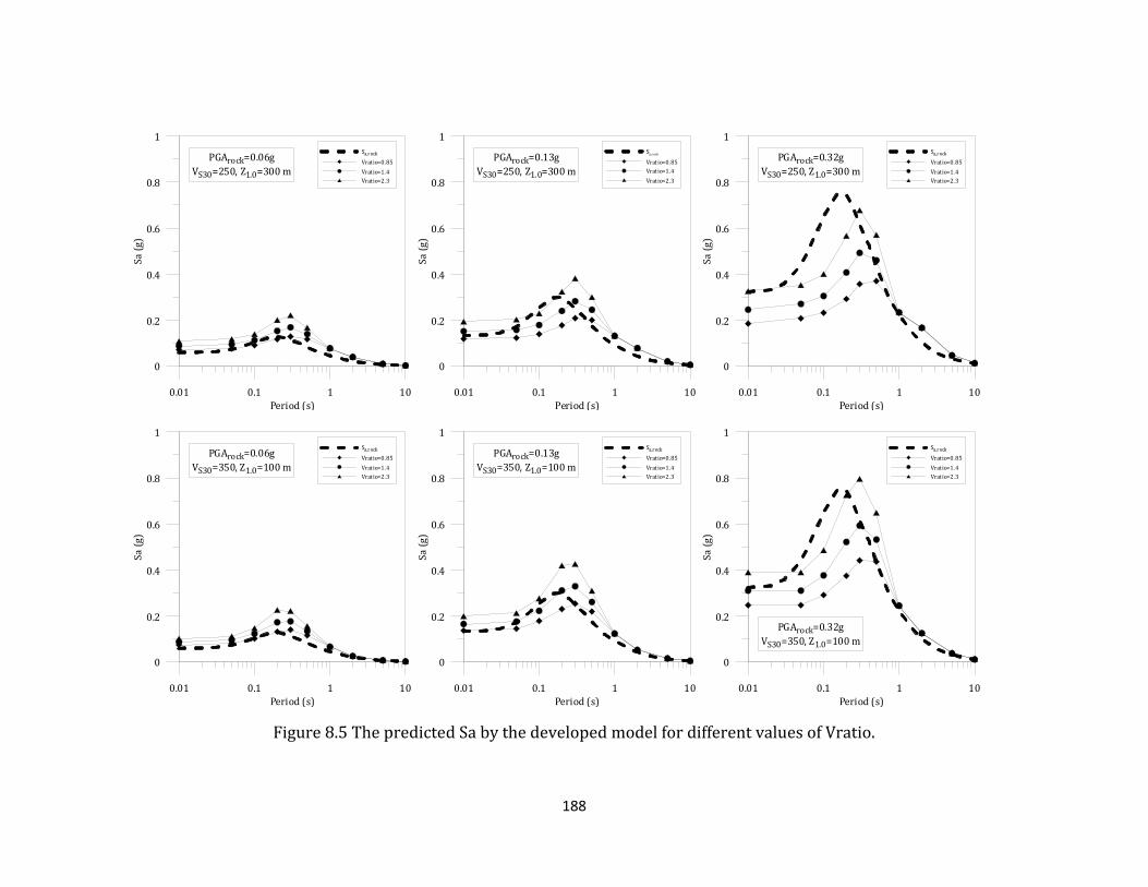
188
0.01 0.1 1 10Period (s)
0
0.2
0.4
0.6
0.8
1S
a(g
)
Sa,rock
Vratio=0.85
Vratio=1.4
Vratio=2.3
PGArock=0.06g
VS30=250, Z1.0=300 m
0.01 0.1 1 10
Period (s)
0
0.2
0.4
0.6
0.8
1
Sa
(g)
Sa,rock
Vratio=0.85
Vratio=1.4
Vratio=2.3
PGArock=0.13g
VS30=250, Z1.0=300 m
0.01 0.1 1 10
Period (s)
0
0.2
0.4
0.6
0.8
1
Sa
(g)
Sa,rock
Vratio=0.85
Vratio=1.4
Vratio=2.3
PGArock=0.32g
VS30=250, Z1.0=300 m
0.01 0.1 1 10Period (s)
0
0.2
0.4
0.6
0.8
1
Sa
(g)
Sa,rock
Vratio=0.85
Vratio=1.4
Vratio=2.3
PGArock=0.06g
VS30=350, Z1.0=100 m
0.01 0.1 1 10
Period (s)
0
0.2
0.4
0.6
0.8
1S
a(g
)
Sa,rock
Vratio=0.85
Vratio=1.4
Vratio=2.3
PGArock=0.13g
VS30=350, Z1.0=100 m
0.01 0.1 1 10
Period (s)
0
0.2
0.4
0.6
0.8
1
Sa
(g)
Sa,rock
Vratio=0.85
Vratio=1.4
Vratio=2.3
PGArock=0.32g
VS30=350, Z1.0=100 m
Figure 8.5 The predicted Sa by the developed model for different values of Vratio.

189
0.01 0.1 1 10Period (s)
0
1
2
3
AF
NGA -Average
Vratio=0.85
Vratio=1.4
Vratio=2.3
PGArock=0.06g
VS30=250, Z1.0=300 m
0.01 0.1 1 10Period (s)
0
1
2
3
AF
NGA -A verage
Vratio=0.85
Vratio=1.4
Vratio=2.3
PGArock=0.13g
VS30=250, Z1.0=300 m
0.01 0.1 1 10Period (s)
0
1
2
3
AF
NG A-Av era ge
Vratio=0.85
Vratio=1.4
Vratio=2.3
PGArock=0.32g
VS30=250, Z1.0=300 m
0.01 0.1 1 10Period (s)
0
1
2
3
AF
NG A-Ave rag e
Vratio=0.85
Vratio=1.4
Vratio=2.3
PGArock=0.06g
VS30=350, Z1.0=100 m
0.01 0.1 1 10
Period (s)
0
1
2
3A
F
NG A-Av erag e
Vratio=0.85
Vratio=1.4
Vratio=2.3
PGArock=0.13g
VS30=350, Z1.0=100 m
0.01 0.1 1 10Period (s)
0
1
2
3
AF
NG A-Ave rag e
Vratio=0.85
Vratio=1.4
Vratio=2.3
PGArock=0.32g
VS30=350, Z1.0=100 m
Figure 8.6 Comparison of the predicted AF by the proposed model and NGA models.

190
8.4 Limitations of the Proposed Model
As previously discussed, soil profiles can experience significantly large shear strains
at high level of shaking. Because the equivalent linear assumption breaks down at
shear strains greater than about 1% and the AF values developed in this study are
all based on equivalent-linear analysis, it is important to identify when excessive
shear strains were induced. The level of generated shear strain in a soil profile
depends on the stiffness of the site and the level of shaking. Softer soil profiles
experience larger strains than stiffer soil profiles subjected to the same level of
input intensity. Figure 8.7 plots strain profiles induced in the softest site considered
in this study (VS30=118 m/s) for four different input intensities. At PGArock=0.1 g, the
maximum generated strain in the site is about 0.4 %. The maximum induced strain
increases as PGArock increases and exceeds 1% for PGArock=0.22 g and larger. This
result indicates that the AF values from this site are not realistic for PGArock greater
than 0.22 g.
The PGArock that first induces maximum shear strains greater than 1% is called
PGArock -1%. This value is compiled for the profiles analyzed and used to identify the
limitations of the developed model. Figure 8.8 plots PGArock -1% versus VS30 for the
soil profiles analyzed in this study. For soil profiles with VS30 less than 200 m/s, the
maximum shear strain exceeds 1% at PGArock =0.22g. The maximum shear strain
exceeds 1% at larger input intensities for stiffer sites (e.g., PGArock -1% ~ 0.4 g for VS30
= 300 m/s, PGArock -1% ~ 1.0 g for VS30 = 400 m/s). For soil profiles with VS30 greater
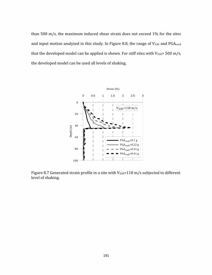
191
than 500 m/s, the maximum induced shear strain does not exceed 1% for the sites
and input motion analyzed in this study. In Figure 8.8, the range of VS30 and PGArock
that the developed model can be applied is shown. For stiff sites with VS30> 500 m/s,
the developed model can be used all levels of shaking.
0 0.5 1 1.5 2 2.5 3
Strain (%)
100
80
60
40
20
0
Dep
th(m
)
PGArock=0.1 g
PGArock=0.22 g
PGArock=0.31 g
PGArock=0.41 g
VS30=118 m/s
Figure 8.7 Generated strain profile in a site with VS30=118 m/s subjected to different level of shaking.
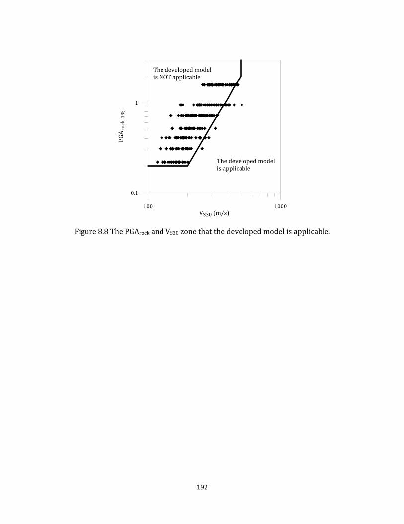
192
Figure 8.8 The PGArock and VS30 zone that the developed model is applicable.

193
8.5 Summary
Amplification factors (AF) and acceleration response spectra (Sa) predicted by the
developed amplification model and the site amplification models of NGA
relationships are compared. The proposed model predicts Sa and AF smaller than
the NGA models at high level of shaking and small VS30. The prediction of the
proposed model approaches the NGA models prediction as input intensity
decreases.
The developed model considers the effect of Vratio in the prediction of
amplification. Amplification for sites with larger Vratio is significantly higher than
for sites with smaller Vratio, resulting in significantly different surface response
spectra. Vratio affects amplification at short periods (T<1.0 s) only.
The developed model is applicable to PGArock smaller than PGArock-1%. PGArock-1%
is the level of input intensity above which the maximum strain exceeds 1%. PGArock-
1% depends on VS30 and increases with the increase of VS30.

194
Chapter 9
Summary, Conclusions, and
Recommendations
9.1 Summary and Conclusions
In this study, an improved site amplification model is developed that considers the
effect of multiple site parameters that affect amplification. This model includes
parameters previously considered in ground motion predictions equations (e.g., VS30
and Z1.0), but also identifies an additional parameter that influences site
amplification.
To identify the appropriate site parameters to be considered, ninety nine soil
profiles were generated manually using five baseline velocity profiles. The top 30 m
of each baseline shear wave velocity profile was modified to maintain the same VS30
but to simulate a different VS structure. The seismic responses of the generated
profiles were analyzed using the equivalent linear approach as implemented in the
site response program, Strata (Kottke and Rathje, 2008). Different site parameters
195
such as Vmin, thVmin, MAXIR and Vratio are considered to investigate the variation in
AF between sites with a common VS30. These analyses identified Vratio as the site
parameter that influences site amplification the most and can explain the variation
in amplification between sites with the same VS30.
To generalize the findings from the analyses in which only the top 30 m of the
velocity profile were varied, a suite of fully randomized velocity profiles are
generated and their responses analyzed using Strata. The results of the site
response analyses conducted on these four hundred fully randomized velocity
profiles confirmed the influence of Vratio on site amplification. The computed
amplification factors were used to develop a functional form that incorporates its
effect. To consider the effect of soil nonlinearity in the developed model, soil profiles
are analyzed under different input rock shaking levels.
The developed amplification model consists of two components; the linear-
elastic and nonlinear components. The computed site amplification under low input
intensity (PGArock=0.01g) are used to develop the linear component of the model
and the higher input intensities are used to develop the nonlinear component.
Vratio affects both the linear and nonlinear behavior of a soil profile; therefore, both
linear and nonlinear components include Vratio in their functional forms.
The effect of Vratio on site amplification is only significant at shorter periods
(T<1.0 s). Therefore, different models are developed for shorter (T<1.0 s) and
longer (T≥ . s) periods. At short periods, the linear-elastic component of the model
196
uses a second-order polynomial functional form for modeling the effect of ln(VS30)
on ln(AF) rather than the linear relationship used in other site amplification models.
The second-order polynomial better fits the AF data at low intensities, particularly
at smaller values of VS30. The linear-elastic model incorporates the effects of Vratio
through a linear relationship between ln(Vratio) and ln(AF). The slope of this
relationship is VS30-dependent. At longer periods, the model uses a linear
relationship between ln(VS30) and ln(AF) rather than a second-order polynomial,
and no Vratio effect is modeled. Additionally, at long periods site amplification is
affected by the depth to bedrock (i.e., Z1.0) in addition to VS30. The effect of Z1.0 is
considered in the linear component of the proposed model because it is not
influenced by soil nonlinearity.
The nonlinear component of the model incorporates the effect of input intensity
on the VS30 and Vratio scaling. The effect of input intensity is coupled with the VS30
scaling by making ln(AF) a function of Sa,rock and VS30. The effect of input intensity on
the Vratio scaling is incorporated by making the relationship between ln(AF) and
ln(Vratio) a function of Sa,rock.
The resulting amplification model accounts for the influence of VS30, Vratio,
Sa,rock, and Z1.0. Generally, larger amplification is predicted for sites with smaller
VS30, larger Vratio, and larger Z1.0. For sites with the same average shear wave
velocity in top 30 m (VS30), a larger value of Vratio indicates a larger change in Vs

197
over the top 30 m. At larger input intensities, the amplification at short periods will
be larger for sites with larger VS30.
The comparison of the developed model with the site amplification models of
NGA prediction equations shows that the developed model predicts smaller site
amplification at high level of shaking for soft sites. Soil profiles under high level of
shaking experience significantly large strain. The equivalent linear assumption is
invalid at strain larger than 1%. Therefore, the developed model, which is based on
site amplification computed by the equivalent linear method, is invalid in these
cases. The shaking level above which the maximum generated shear strain in a
profile exceeds 1% is VS30 dependent. The application of the proposed model should
be limited to the range of shaking level and VS30 that the assumption of the
equivalent linear method is valid.
9.2 Recommendations for Future Work
The model developed in this study is based on numerical simulations of site
amplification and can be expanded in various ways. To provide more valid
amplification predictions at small VS30 values, nonlinear site response analyses
should be performed and the computed amplification factors for these sites should
be used in the development of the site amplification model. These data would be
most important to include for moderate to large input intensities.

198
To evaluate the developed model and the relationship between Vratio and
ground shaking, recorded strong motion data at sites with measured VS profiles
should be considered. The predicted response spectral values for each recording
from a ground motion prediction equation can be computed for the associated
magnitude, distance VS30, etc. and the residual computed with respect to the
recorded value. The relationship between the residuals and the computed values of
Vratio for each site can be investigated to confirm the influence of Vratio on
recorded ground motions and to evaluate the functional form of the relationship
between ln(AF) and ln(Vratio). Recordings at borehole arrays site, in which
recordings are made at the ground surface and at some depth within the bedrock,
can also be used to directly compute amplification factors. In this case, the
relationship between amplification and Vratio can be investigated directly.
199
Bibliography N. Abrahamson and W. Silva. Abrahamson and Silva NGA ground motion relations for the geometric mean horizontal component of peak and spectral ground motion parameters. PEER report200x/xx, University of California, Berkeley, July 2007.
N. Abrahamson and W. Silva. Summary of the Abrahamson and Silva ground motion relationships. Earthquake Spectra, 24(1):67-97, February 2008.
N. Abrahamson, G. Atkinson, D. Boore, Y. Bozorgnia, K. Campbell, B. Chiou, I.M. Idriss, W. Silva, and R. Youngs. Comparison of the NGA ground motion relations. Earthquake Spectra, 24(1):45-66, February 2008.
S. Barani, R. De Ferrari, G. Ferretti, and C. Eva. Assessing the effectiveness of soil parameters for ground response characterization and classification. Earthquake Spectra, 24(3):565-597, August 2008.
P. Bazzuro and C.A. Cornell. Ground motion amplification in nonlinear soil sites with uncertain properties. . Bulletin of Seismological Society of America, 94(6):2090-2109, December 2004.
D.M. Boore and G.M. Atkinson. Ground-motion prediction equations for the average horizontal component of PGA, PGV, and 5%-damped PSA at spectral periods between 0.01s and 10.0 s. Earthquake Spectra, 24(1):99-138, February 2008.
K.W. Campbell and Y.Bozorgnia. NGA Ground motion model for the geometric mean horizontal component of PGA, PGV, PGD, and 5% damped linear elastic response spectra for periods ranging from 0.01 to 10 s. Earthquake Spectra, 24(1):139-171, February 2008.
K.W. Campbell and Y. Bozorgnia. Updated near source ground motions (attenuation) relations for the horizontal and vertical components of peak ground acceleration and acceleration response spectra. Bulletin of Seismological Society of America, 93(1):314-331, February 2003.
K.W. Campbell. Emperical near-source attenuation relationships for horizontal and vertical components of peak ground acceleration, peak ground velocity, and pseudo-

200
absolute acceleration response spectra. Seismological Research letters, 68(1):154-179, January/ February 1997.
B.S.J. Chiou and R.R.Youngs. An NGA model for the average horizontal component of peak ground motion and response spectra. Earthquake Spectra, 24(1):173-215, February 2008.
B. Chiou, R. Darragh, N. Abrahamson, and W. Silva. NGA project strong motion database. Earthquake Spectra, 24(1):23-44, February 2008.
Y. Choi and J.P. Stewart. Nonlinear site amplification as function of 30 m shear wave velocity. Earthquake Spectra, 21(1):1-30, February 2005.
C.J. Costantino, E. Heymsfield, and Y.T. Gu. Site specific estimates of surface ground motions for the K-reactor site, Savannah River Plant. Upton, New York: Structural Analysis Division, Nuclear Energy Department, Brookhaven National Laboratory, 1991.
M.B. Darendeli. Development of s new family of normalized modulus reduction and material damping curves. Austin, Texas: The University of Texas,2001.
J.L. Devore. Probability and statistics for engineering and science. Third Edition. Brooks/Cole Publishing Company, Pacific Grove, Clifornia, 1990.
I.M. Idriss. An NGA empirical model for estimating the horizontal spectral values generated by shallow crustal earthquakes. Earthquake Spectra, 24(1):217-242, February 2008.
A.R. Kottke and E.M. Rathje. Technical manual for strata. PEER 2008/10 publication, University of Texas, Austin, February 2009.
A.R. Kottke, Site amplification model considering VS30 and depth, unpublished report, October 2011.
S.L. Kramer. Geotechnical earthquake engineering. Prentice Hall, Saddle River, New Jersey, 1996.
R.K. McGuire, G.R. Toro, T.P. O’Hara, J.P. Jacobson, and W.J. Silva. Probabilistic seismic hazard evaluation at nuclear plant sites in the Central and Eastern United States: Resolution of the Charleston Earthquake Issue. Palo Alto, California: Electric Power Research Institute, 1989.
R. Ramanathan. Introductory econometrics with applications. Fourth Edition. The Dryden Press, Harcourt Brace College Publishers, 1998.
A. Rodriguez-Markez, J.D. Bray, and N.A. Abrahamson. An empirical geotechnical seismic site response procedure. Earthquake Spectra, 17(1): 65-87, February 2001.
201
W.J. Silva. Site response simulations for the NGA project. University of California, Berkeley, 2008.
J.P. Stewart, A.H. Liu, and Y. Choi. Amplification factors for spectral acceleration in tectonically active regions. Bulletin of the Seismological Society of America, 93(1), 332-352, February 2003.
G.R. Toro. Probabilistic models of site velocity profiles for generic and site-specific ground-motion amplification studies. Upton New York: Brookhaven National Laboratory, 1995.
G.R. Toro, W.J. Silva, R.K. McGuire, and R.B. Hermann. Probabilistic seiemic hazard mapping of the Mississippi embayment. Seismological Research Letters, 63(3),449-475,1992
M. Walling, W. Silva, and N. Abrahamson. Nonlinear site amplification factors for constraining the NGA models. Earthquake Spectra, 24(1):243-255, February 2008.


