Embed Size (px)
Citation preview

DEVELOPMENT OF LAND-USE MAP FOR SALT RIVER BASIN
USING SATELLITE IMAGERY
A Thesis
presented to
the Faculty of the Graduate School
at the University of Missouri
In Partial Fulfillment
of the Requirements for the Degree
of Master of Science
by
ANH THI TUAN NGUYEN
Allen Thompson, Thesis Supervisor
DECEMBER 2010

The undersigned, appointed by the Dean of the Graduate School, have examined the thesis
entitled:
DEVELOPMENT OF LAND-USE MAP FOR SALT RIVER BASIN
USING SATELLITE IMAGERY
Presented by Anh Nguyen Thi Tuan
a candidate for the degree of Master of Science
and hereby certify that in their opinion it is worthy of acceptance
_____________________________________
Thompson Allen, Biological Engineering Department
_____________________________________
Kenneth Sudduth, Biological Engineering Department
_____________________________________
Cuizhen (Susan) Wang, Geography Department

ii
ACKNOWLEDGEMENTS
I would like to thank my committee for their encouragement and enthusiasm
throughout my time at the University of Missouri. My research would not have been possible
without the help and support of many people. I am grateful to my advisor, Dr. Allen
Thompson, for encouraging this work and his support of my effort. To my committee
members: Dr. Ken Sudduth and Cuizhen Wang for their willing guidance and remote sensing
expertise. Financial support was provided by the MOET program that gave me the
opportunity to study in the Biological Engineering Department.
I wish to express gratitude to Prof. Joseph Hobbs for his encouragement and support
through the duration of my studies. I also wish to thank the staff at the University of Missouri
Columbia for their assistance, advice and guidance through my academic program. My
efforts have been influenced by many instructors in the departments of Biological
Engineering, Geography and Forestry with whom I have completed course-work during my
past two and half years. My knowledge and abilities have been greatly enhanced by their
efforts.
I wish to express my special thanks and gratitude to Daniel Seidel, Dylan Caspari,
Josh Kezer, Jared Caspari, Jean Elizabeth, Trang Tran, Truc Bui, Anh Phan, Quang Nguyen,
Giang Nguyen, BaoAnh Nguyen, Dung Tran and Nguyen Doan for their understanding,
sharing, and support throughout the duration of my studies at the University of Missouri.
I would like to thank all the staff at the International Center for their help, support and
promoting the chance to experience American education and culture firsthand and to share

iii
my own cultures. Thanks for providing a variety of workshops, events, volunteer
opportunities and outreach programs and involving me with the global campus.
Finally, this thesis would not have been possible without the constant support and
encouragement of my parents and my family. I thank my parents, my sister Nguyet Nguyen
and my brother Tuan Nguyen for believing in me and encouraging me to study abroad.

iv
TABLE OF CONTENTS
ACKNOWLEDGEMENTS ....................................................................................................... ii
LIST OF TABLES .................................................................................................................... vi
LIST OF FIGURES ................................................................................................................. vii
ABSTRACT ..............................................................................................................................ix
Chapter 1 INTRODUCTION ............................................................................................................... 1
1.1 Research objectives ..................................................................................................... 3
2 LITERATURE REVIEW .................................................................................................... 4
2.1 Remote Sensing ........................................................................................................... 4
2.1.1 Landsat Thematic Mapper History ......................................................................6
2.1.2 Moderate Resolution Imaging Spectrometer (MODIS) .......................................9
2.2 Land cover classification ........................................................................................... 10
2.3 Methods of classification ........................................................................................... 10
2.3.1 Object-based versus pixel-based classification ..................................................11
2.3.2 Supervised classification methods .....................................................................12
2.3.3 Unsupervised classification methods .................................................................13
2.3.4 Ground truth data ...............................................................................................13
2.4 Vegetation indices (VI) ............................................................................................. 14
2.4.1 Normalized Difference Vegetation Index (NDVI) ............................................14
2.4.2 TM Tasseled cap ................................................................................................16
2.4.3 Principal component transform ..........................................................................17
2.5 Applications of NDVI ............................................................................................... 17
2.6 GIS and Remote Sensing Software ........................................................................... 19
3 METHODOLOGY ............................................................................................................ 21
3.1 Study site ................................................................................................................... 21
3.1.1 Summer crops ....................................................................................................23

v
3.1.2 Winter crops .......................................................................................................26
3.1.3 Grass/Pasture hay ...............................................................................................27
3.1.4 Other features .....................................................................................................28
3.2 Materials .................................................................................................................... 28
3.2.1 Reference data ....................................................................................................29
3.3 Image Preprocessing .................................................................................................. 35
3.4 Previous crop discrimination study on the Salt River watershed .............................. 36
3.5 Image Processing ....................................................................................................... 38
3.5.1 Class Identification Process ...............................................................................39
4 RESULTS AND DISCUSSION ........................................................................................ 40
4.1 Analysis ..................................................................................................................... 40
4.1.1 Analysis of Landsat data in 2006 .......................................................................40
4.1.2 Analysis of Landsat data in 2005 .......................................................................41
4.1.3 Crop NDVI profiles ...........................................................................................43
4.2 Decision tree rules ..................................................................................................... 47
4.2.1 Decision rules to separate water and urban/soil from the others .......................47
4.2.2 Decision rules to separate winter wheat and double crop from the other
land uses ............................................................................................................48
4.2.3 Decision rules to separate corn from the other summer crops ...........................49
4.2.4 Decision rules to separate soybean and grain sorghum .....................................49
4.3 Accuracy assessment ................................................................................................. 50
4.4 Crop type maps .......................................................................................................... 60
5 SUMMARY AND CONCLUSION .................................................................................. 64
5.1 Future work ............................................................................................................... 65
APPENDIX A ......................................................................................................................... 67
APPENDIX B ......................................................................................................................... 77
APPENDIX C ......................................................................................................................... 82
REFERENCES ....................................................................................................................... 89

vi
LIST OF TABLES
Table Page
2.1 Relationship between scale and spatial resolution in satellite-based land cover mapping programs (Franklin, 2002) ................................................................................7
2.2 Thematic Mapper Spectral Bands (adapted from Lillesand, 2004) .....................................8
2.3 Selected remote sensing Vegetation Indices (adapted from Jensen, 2000) .......................15
3.1 Gradients, basin area and percentages of cover types in the Upper Salt River Basin in 1990 (Skadeland, 1992) .................................................................................................22
3.2 USDA NASS county statistics (2000) ...............................................................................32
3.3 USDA NASS county-level crop statistics for 2005 (acres) ...............................................32
3.4 USDA NASS county-level crop statistics for 2006 (acres) ...............................................33
4.1. Accuracy assessment resulting from classifying the crop map in 2005 for the Greenley reference area .................................................................................................54
4.2 Accuracy assessment resulting from classifying the crop map in 2005 for the Goodwater creek sub-basin ...........................................................................................55
4.3 Accuracy assessment resulting from classifying the crop map in 2006 for the Greenley reference area .................................................................................................56
4.4 Accuracy assessment resulting from classifying the crop map in 2006 for the Goodwater creek sub-basin ...........................................................................................57
4.5 Accuracy assessment resulting from classifying the crop map in 2006 for the Salt River Basin watershed ...................................................................................................58
4.6 Crop area comparison between map statistic and NASS crop area statistic in 2005 .........59
4.7 Crop area comparison between map statistic and NASS crop area statistic in 2006 .........59

vii
LIST OF FIGURES
Figure Page
3.1 Salt River Basin (Lerch et al., 2008) ..................................................................................23
3.2 Corn Growth Stage Development (Source: http://weedsoft.unl.edu/documents/GrowthStagesModule/Corn/Corn.html#) ..............24
3.3 Soybean Growth Stage Development (Source: http://weedsoft.unl.edu/documents/GrowthStagesModule/Soybean/Soy.html#) ..........25
3.4 Grain Sorghum Growth Stage Development (Source: http://weedsoft.unl.edu/documents/GrowthStagesModule/Sorghum/Sorg.html#) .......26
3.5 Winter Wheat Growth Stage Development (Source: htttp://weedsoft.unl.edu/documents/GowthStagesModule/Wheat/Wheat.html#) .........27
3.6 (a) A mosaic of Landsat TM row 32 and 33 path 25 (23 May 2005) and (b) Salt River Basin county-boundary. ......................................................................................30
3.7 False color Landsat image for 23 May 2005 subset to the county boundary of Salt River Basin. ...................................................................................................................31
3.8 USDA NASS CDL map subset to the Salt River Basin (2006). ........................................34
3.9 The 23-band NDVI trend curve of sample pixel before and after smoothing (extract from ENVI through 2-profile spectral curve). ...............................................................37
4.1 MODIS Winter Wheat NDVI profile in 2006. ..................................................................44
4.2 MODIS Corn NDVI profile in 2006. .................................................................................44
4.3 MODIS Soybean NDVI profile in 2006. ...........................................................................45
4.4 MODIS Sorghum NDVI profile in 2006. ..........................................................................45
4.5 MODIS Forest NDVI profile in 2006. ...............................................................................46

viii
4.6 MODIS Grass NDVI profile in 2006. ................................................................................46
4.7 Decision rules to define water for 2005 .............................................................................48
4.8 Salt River Basin watershed crop map (2005). ...................................................................62
4.9 Salt River Basin watershed crop map (2006). ...................................................................63
A.1 Decision tree for 2005 crop map. ......................................................................................68
A.2 Decision tree for 2006 crop map. ......................................................................................73
B.1 Goodwater creek Sub-basin 2005. ....................................................................................78
B.2 Greenley reference area 2005. ...........................................................................................79
B.3 Goodwater creek Sub-basin 2006. ....................................................................................80
B.4 Greenley reference area 2006. ...........................................................................................81
C.1 Missouri Initial planting dates – corn – 2005 crop year ....................................................83
C.2 Missouri Initial planting dates – grain sorghum – 2005 crop year. ...................................84
C.3 Missouri Initial planting dates – soybean – 2005 crop year. .............................................85
C.4 Missouri Initial planting dates – corn – 2006 crop year. ...................................................86
C.5 Missouri Initial planting dates – grain sorghum – 2006 crop year. ...................................87
C.6 Missouri Initial planting dates – soybean – 2006 crop year. .............................................88

ix
DEVELOPMENT OF LAND-USE MAP FOR SALT RIVER BASIN
USING SATELLITE IMAGERY
Anh Nguyen
Allen Thompson, Thesis Supervisor
ABSTRACT
The Salt River watershed is located in northeastern Missouri. Outflows from the
watershed drain into Mark Twain Lake, the major water supply source for people in the
region. Since most of the land use in the watershed is cropland and grass, an evaluation for
possible improvement of watershed management is encouraged. However, there is a lack of
field/survey information concerning the crops in previous years necessary to build a long term
simulation and to validate the long term trend of pollutant concentrations. A potential method
to aid land-use evaluation is the use of satellite imaging data. Satellite remote sensing data
have many advantages compared with other data sources, such as field methods, or aerial
photography and have been widely used in land cover classification. It provides the capability
to evaluate dynamic landscape pattern and observe changes and trends across a large scale
pattern through time. The overall objective of this study was to apply Landsat 5 Thematic
Mapper (TM) data to build crop type maps for Salt River Basin for a two-year period (2005-
2006) useful in evaluating land-use management. Decision tree analysis, combination of pixel
and object based methods, was applied. Ground truth data in Goodwater creek sub-basin and
Greenley reference area were used to assess the accuracy of the procedure, and crop acreage
estimates were compared to county-level statistics. Crop type classification of 2005 had
higher accuracy than that of 2006 because there was more in-season Landsat data obtained in
2005. However, this method was efficient in classifying crops when there was lack of cloud-
free images in growing season with an overall accuracy was 90% in 2006. Additional testing
of this method could result in a robust technique for crop classification for specific crops in
cloud-free-limited Landsat data for applying to other study.

1
Chapter 1
INTRODUCTION
The Salt River basin is located in northeastern Missouri. The closing of Clarence
Cannon Dam in 1983 formed the Mark Twain Lake. The total catchment area is
approximately 6417 km2. River and stream outflow from the watershed drain into Mark
Twain Lake, the major water supply source for people in the region. Since the dam was
closed, the Lake has been receiving sediment in the watershed, including inorganic sediment
loading, which can degrade water quality. Concerning these soil and water quality problems,
the Salt River was selected as one of the USDA Agricultural Research Service benchmark
watersheds for Conservation Effects Assessment Project (CEAP) (Lerch et al, 2008). Since
most of the land use in the watershed is cropland and grass, an evaluation for improvement of
watershed management is possible. Previous research in the watershed area included
quantifying the nutrient and sediment concentrations in five major tributaries in the Upper
Salt River Basin and ten small tributaries in the Middle Fork of the Salt River (Skadeland,
1992) ; applying Remote Sensing of Suspended solid and Turbidity in Mark Twain Lake,
Missouri (Allen, 2000). Ghidey et al. (2005) had built a model to simulate hydrology and
water quality for a claypan soil watershed and scaled up the SWAT (Soil and Water
Assessment Tool) model from Goodwater Creek (Ghidey et al, 2007). Results from the
SWAT model showed that the simulation model can be used for a long term estimation of
contaminant concentration. However, there is a lack of field/survey information concerning
the crop types that were planted in previous years in order to build a long term simulation
model and to validate the long term trend of pollutant concentrations. Land use is an

2
important input to the SWAT model. Cropland Data Layer (CDL) produced by National
Agricultural Statistic Service (NASS), based on NASS annual sampling data. Thus, the
requirement to develop a crop map for the watershed area is justified, especially for the
previous years.
Since satellite remote sensing data have many advantages compared with other data
sources, such as field methods, and aerial photography, it has been used widely in land cover
classification. It is useful in evaluating temporal and spatial effects. Temporal effects show
the change of feature spectral characteristics over time. Spatial effects help to analyze factors
with a similar characteristic feature at a given point of time but at different geographic
locations. The other advantage of remote sensing is that it can offer cost-effective means of
providing more frequent crop/land cover data for short and long term planning. It provides
the capability to evaluate dynamic landscape patterns and to observe changes and trends
across a large scale pattern through time. It also provides spatially and temporally
comprehensive data (Franklin, 2001; Jensen, 2005). Using the information from remote
sensing satellites properly would be very useful for managers to be able to understand natural
impacts and to solve many environmental issues. The advantage of difference in spectral of
objects can help to discriminate between objects in the area. However, there are several
factors that can affect a feature’s reflectance. Remote sensing techniques provide a synoptic
view of an area and methods utilizing remote sensing data in deterministic models can
potentially supply new information.
The purpose of this study is to apply Landsat 5 Thematic Mapper (TM) data to build
crop type maps for the Salt River Watershed for two previous years (2005- 2006). The study
also applies the Normalized Difference Vegetation Indices derived from MODIS as a

3
reference to build the hypothesis for differentiating among crop types during the growing
season.
1.1 Research objectives
The overall objective of this study was to develop land cover/land use maps for Salt
River basin from remote sensing data. Specifically, the objectives were to:
• Find the most appropriate method to delineate crop types in the agricultural land in
Salt River basin under conditions of limited field data.
• Analyze and determine crop phenological behaviors in Salt River basin.
• Develop land cover maps from this watershed area for years 2005 and 2006

4
Chapter 2
LITERATURE REVIEW
2.1 Remote Sensing
Applying satellite remote sensing data is the process of analyzing data from satellite,
which collects spectral information about an object, area, or phenomenon without contacting
the object, area, or phenomenon. Satellite imagery uses electromagnetic energy sensors to
obtain reflectance data from features on earth.
Remote sensors collect radiation reflectance from features at a distance which crosses
through a path length of the atmosphere and is affected by atmospheric scattering and
absorption. Atmospheric scattering is the unpredictable reflectance of radiation by particles
in the atmosphere (Rayleigh scatter, Mie scatter, non selective scatter) (Jensen, 2000).
Conversely, atmospheric absorption is the phenomena of loss energy due to atmospheric
particles, such as water vapor, carbon dioxide and ozone.
Spectral reflectance of an object varies as a function of wavelength which can help to
discriminate objects in the area. For example, healthy green vegetation can be classified from
dry bare soil and clear lake water since water has low reflectance in visible wavelength and
no reflectance in near IR wavelength, while bare soil has higher reflectance than vegetation
in visible wavelength but less in the near infrared (IR) wavelength. Moreover, the healthy
green vegetation spectral curve has a “peak and valley” that can be easily identified.
(Lillesand, 2004) Although the reflectance of individual features varies along the spectrum,
the curves exhibit some elementary points concerning spectral reflectance. Some factors
affect the feature’s reflectance. For example, the near IR reflectance of vegetation increases

5
with the number of leaf layers in a canopy, with a maximum reflectance at about eight layers
of leaves (Bauer, 1985). Soil reflectance is affected by the presence of iron oxide, organic
matter content or moisture content. Soil texture and surface roughness are two factors that
influence soil reflectance as well. Soil with low moisture content and coarse texture has a
high reflectance, while an increase in organic content in the soil reduces reflectance.
(Lillesand, 2004)
Water absorbs radiation strongly at water absorption bands, located at 1.4, 1.9 and 2.7
m. This characteristic helps to locate and define water bodies within the area. However, the
water reflectance is affected by solid material within the water. When the turbidity of water
increases, reflectance also increases. Lyon et al. (1988) used the data from multiple days
Landsat and AVHRR to determine suspended sediment concentration based on this feature of
water reflectance. Choubey and Subramanian (1992) used data from India Remote Sensing
Satellite-1A to investigate this character of water turbidity to estimate suspended solids.
Thus, in order to operate efficiently, the knowledge and understanding of spectral
characteristics of the particular features under investigation, as well as what factors influence
these characteristics are required. Also, information about vegetation water content allows
the user to infer water stress for irrigation decisions. Jackson et al. (2004) explored the
potential of using remote sensing derived the normalized difference water index, to map and
monitor corn and soybean.
Another advantage of satellite remote sensing data is its usefulness in evaluating
temporal and spatial effects. Temporal effects show the change of feature spectral
characteristics over time. Spatial effects help to analyze factors with a similar characteristic
feature at a given point of time but at different geographic locations. In addition, the energy

6
recorded is affected by the atmosphere through which the radiation passes. Atmospheric
correction models are built to correct these types of errors.
Image processing systems contain algorithms to remove or reduce atmospheric affect.
The simplest and commonly used model for atmospheric correction is DOS (Dark Object
Subtraction) with the assumption that atmospheric effects are the same for all pixels in the
image and dark objects (clear water bodies) have homogeneously zero radiance for all bands.
The procedure requires checking the visible band radiances over the lake or other dark
objects and adjusting the observed value to more closely match the expected reflectance.
One of the most common applications of remote sensing is land cover classification,
the process of assigning a particular class to an image object or pixels in the image (Cihlar,
2000; Foody, 2002). Land cover classification can be applied at different scales, from
continental and global level scales (Friedl et al., 1999; Agrawal et al., 2003; Joshi et al.,
2006) to local regional studies (Brook and Kenkel, 2002; Reese et al., 2002; Van Niel and
McVicar, 2004). The Landsat imagery is commonly used for medium resolution land cover
classification. Another application of crop mapping include estimating crop yield
(Doraiswamy et al., 2006; Wang et al., 2005), water content (Jackson et al., 2004), crop
estimation (Craig, 2001) as well as simple crop classification (Yamamoto et al., 2009). The
relationship between level scale and spatial resolution in satellite-based land cover mapping
is listed in Table 2.1.
2.1.1 Landsat Thematic Mapper History
The Landsat 5 Thematic Mapper (TM) and the Landsat 7 Enhanced Thematic Mapper
Plus (ETM+) have repetitive, circular, sun-synchronous, near polar orbits with a 16-day

7
repeat cycle for each satellite. Both of them are 8-bit, moderate resolution sensor (30m
resolution). In 2003, an instrument anomaly was detected onboard the satellite that collects
Landsat 7 ETM+ data. The SLC failure of Landsat 7 ETM+ has forced users to rely on the
Landsat 5 TM data for most Landsat image requirements. The TM sensor collects data in
seven bands (Table 2.2). Both the TM mid-IR bands (bands 5 and 7) are sensitive to plant
water stress (Lillesand, 2004). Plant stress classification is also aided by TM band 1. For a
mapping of water sediment pattern, a normal color composite of bands 1, 2 and 3 (Blue
Green Red) is preferred. For vegetation discrimination, the combination of visible bands
(bands 1-3) with near IR (band 4) and mid IR (bands 5-7) are very helpful.
Table 2.1 Relationship between scale and spatial resolution in satellite-based land cover mapping programs (Franklin, 2002)
Low spatial
resolution imagery
study phenomena that can vary over 100s or 1000s of meters (small scale)
and could be supported with GOES, NOAA AVHRR, EOS MODIS, SPOT
VEGETATION sensor data
Medium spatial
resolution
study of phenomena that can vary over 10s or 100s of meters (medium
scale) typically with imagery from sensors on the Landsat, SPOT, IRS,
JERS, ERS, Radarsat and Shuttle platforms
High spatial
resolution
study of phenomena that can vary over scales of centimeters to meters
(large scale), are currently supported by aerial remote sensing platforms,
IKONOS and very specific applications of coarse resolution satellite
imagery (e.g., coarse pixels resolution unmixing studies)

8
Table 2.2 Thematic Mapper Spectral Bands (adapted from Lillesand, 2004)
Band Wavelength
(m)
Nominal Spectral
Location
Principal Application
1 0.45 – 0.52 Blue Designed for water body penetration, making it
useful for coastal water mapping. Also useful for
soil/vegetation discrimination, forest-type mapping,
and cultural feature identification
2 0.52 – 0.60 Green Designed to measure green reflectance peak of
vegetation for vegetation discrimination and vigor
assessment. Also useful for cultural feature
identification
3 0.63 – 0.69 Red Designed to sense a chlorophyll absorption region
aiding in plant species differentiation. Also useful
for culture feature identification
4 0.76 – 0.90 Near IR Useful for determining vegetation types, vigor, and
biomass content, for delineating water bodies, and
for soil moisture discrimination
5 1.55 – 1.75 Mid IR Indicative of vegetation moisture content and soil
moisture. Also useful for differentiation of snow
from clouds
6a 10.4 – 12.5 Thermal IR Useful in vegetation stress analysis, soil moisture
discrimination, and thermal mapping application
7a 2.08 – 2.35 Mid IR Useful for discrimination of mineral and rock types.
Also sensitive to vegetation moisture content
aBands 6 and 7 are out of wavelength sequence because band 7 was added to the TM later in the
original system design process

9
Landsat image interpretation has been widely used in many fields, such as agriculture,
cartography, civil engineering, environmental monitoring, forestry, geography, land use
planning and oceanography. However, there is a problem with applying Landsat 5 TM,
because of the low temporal resolution (16 days temporal resolution). Limitation of high
spatial resolution data includes data cost and infrequency.
2.1.2 Moderate Resolution Imaging Spectrometer (MODIS)
MODIS has a much wider field of view than Landsat which gives a greater swath
width and also has a higher temporal resolution. For certain time-sensitive applications, such
as crop mapping during the growing season, a frequent revisit cycle is very important.
MODIS provides a long term observation which is very useful to enhance knowledge of
global dynamics and processes (SBRC, 1994). MODIS views the entire surface of the Earth
everyday. This feature of MODIS was used in many studies of large scale mapping
(Doraiswamy et al., 2006; Wardlow et al., 2007; Chang, 2007). Doraiswamy et al. (2006)
used MODIS Terra data at 250m resolution to classify crop area in four provinces of Brazil
that are the major soybean producing area and demonstrate that MODIS imagery can be used
for regional classification when screened for data anomalies and affected by clouds or
compositing procedures. He also concluded that frequency of MODIS data acquisition at
250m pixel resolution can be used for operational yield prediction programs. The MODIS
sensor offers an option for dealing with some mapping criteria. However, the MODIS pixel is
much larger than the 30m Landsat pixels used for creating maps – therefore, merging these
large pixels into the existing map would generate a significant error to the map quality.

10
2.2 Land cover classification
Analysis of data from satellite remote sensing is widely used, especially for land use -
land cover classification. It is the process of assigning all pixels in the image to a particular
class or theme based on their specific spectral information with different spectral bands from
the satellite sensor. Each type of satellite has several wave bands with specific wavelengths
that collect the level of reflected solar radiation. By spatially and spectrally enhancing an
image, the pattern can be recognized by the human eye. Remote sensing of cropland has been
used a variety of methods and techniques, including multi-temporal analysis, object-based
analysis, and classification methods such as supervised and unsupervised approaches.
2.3 Methods of classification
The overall objective of classification is to categorize all pixels in an image into land
cover classes. Different features have different combinations of Digital numbers (DNs) based
on their spectral reflectance and emission. Applying remote sensing data to separate
vegetative types is studied, especially for agricultural croplands (Franklin and Wulder, 2003).
In an agriculture crop survey, distinct spectral and spatial changes during a growing season
can help to discrimination multi-date imagery which is very difficult when using a single-
date image, because they include different vegetation types which often show a similar
spectral response, resulting from a similar leaf area index value and internal structure.
There are many different techniques to combine and analyze multi-temporal scenes
(Van Niel and McVicar, 2004). Moreover, multi-temporal techniques can increase the
accuracy of the classification process (Murthy et al., 2003; Van Niel and McVicar, 2004).
Van Niel and McVicar (2004) also noticed that a minimum of two and preferably three

11
images taken over a single growing season are necessary to distinguish many different crop
and grassland types. With coarse spatial resolution images and high temporal resolution as
MODIS, it is possible to generate a cloud-free image for a growing season, but it’s rather
difficult to get cloud-free images with Landsat (30m spatial resolution 16-day temporal
resolution).
There are two types of classification techniques: object-based classification and pixel-
based classification. Most traditional remote sensing classification is pixel-based. Aplin and
Atkinson (2001) applied the object-based classification as a method to improve accuracy.
2.3.1 Object-based versus pixel-based classification
Object-based classification divides the satellite image into an object or segments that
represent a homogenous unit on the ground. The entire object is classified based on the
overall statistical properties of the pixels that make up the object rather than classifying each
pixel separately as in pixel-based classification (McIver and Friedl, 2002). The difficulty of
object-based is the establishment of significant objects. It is not possible to hand digitize for
large areas. All natural boundaries may not be found, and those found may not match real
world objects. It requires a laborious set of training data and prior knowledge of the area to
correctly use this method. In addition, features such as roads or streams may be included in
other objects (De Wit and Clevers, 2004). Thus, it results in overestimation or
underestimation of the area.
There are two main weakness of the pixel-based method. The first weakness is that
the products do not express the actual landscape structure well. The second weakness is the
occurrence of mixed pixels within a homogenous field and problems with the edge pixels.

12
Object-based classification is usually combined with other techniques and can be separated
into two main types: supervised classification and unsupervised classification. The difference
between these two techniques is that supervised classification involves a training step
followed by a classification step (priori process). In the unsupervised classification approach,
pixels are grouped based on image statistics first. Then the analyst labels these spectral
groups (called clusters) by comparing the classified image data to ground reference data
(post-prior process).
2.3.2 Supervised classification methods
There are two basic types of supervised classification: parametric method and non-
parametric method. The commonly used parametric supervised classification is Gaussian
Maximum Likelihood Classifier (MLC). The MLC quantitatively evaluates both the variance
and covariance of the category spectral response pattern with the assumption that the
category training data are distributed normally. The unclassified pixels from the image are
assigned to the class for which they have the highest membership probability. Non-
parametric methods make no assumption about statistical distribution of the data. This is the
advantage of the non-parametric supervised classification method; however, it is dependent
on the training data conditions. The non-parametric method includes a decision tree (Franklin
et al., 2002; Jang et al., 2009). The decision tree method has some advantages (Franklin and
Wulder, 2003; Chubey et al., 2006), such as:
- Possible handling high-dimension data set, include non-remotely sensed data as an
aid in classification
- Possible to do with both categorical and continuous data

13
- No assumption about statistical distribution of data
- Has been shown to outperform both MLC and non-parametric classifiers (Chubey et
al., 2006)
However, decision trees rely on the quality of the training data and knowledge about
the objects and factors that affect the objects’ characteristics.
2.3.3 Unsupervised classification methods
Unsupervised classifiers do not utilize training data as the basis of classification.
Classes from unsupervised classification are spectral classes, because they are based on the
natural groupings in the image values. The analyst compares the data with some form of
reference data to determine the identity and informational value of spectral classes. There are
several clustering algorithms that can be used for spectral grouping. One common form is
called “K-means” approach. Each pixel is assigned to the cluster whose arbitrary mean vector
is closest. After all pixels have been classified, revised mean vectors for each cluster are
computed and then the revised means are used as the basis to reclassify the image data. The
procedure continues until there is no significant change in the location of the class mean
vector between successive iteration of the algorithm. ISODATA (Iterative Self-Organizing
Data Analysis) is a widely used “K-means” method for unsupervised classification (Tou and
Gozalez, 1974). This algorithm permits the number of clusters to change from iteration to
the next iteration by merging, splitting and deleting clusters (Lillesand et al., 2004).
2.3.4 Ground truth data
The class maps from supervised or unsupervised classification can be validated with
ground truth data. Ground truth data – reference data may be collected from measurements or

14
observations about the objects, area or phenomena. It can be derived from different sources.
For example, it could be a survey map, laboratory report or aerial photograph. These data are
used to calibrate a sensor, to verify information extracted from remote sensing data and to
help in analysis and interpretation of remote sensing data. Reference data can be very
expensive and time consuming to properly collect (Lillesand et al., 2004).
2.4 Vegetation indices (VI)
Before the launch of Landsat satellites, the idea of using spectral reflectance ratio of
NIR (0.75 m) to red (0.65 m) was presented by Birth and McVey (1968), which they
called the turf color index. Nowadays, formulas combining NIR and Red reflectance are
commonly referred to as spectral vegetation indices. There are more than 20 vegetation
indices in use. A summary of selected VI are in Table 2.3. Vegetation indices were applied to
satellite remote sensing data, which is called the normalized difference vegetation index
(NDVI).
2.4.1 Normalized Difference Vegetation Index (NDVI)
The Normalized Difference Vegetation Index was developed by Rouse et al. (1974)
defined as
NDVI = [NIR - red] / [NIR + red] (2.1)
Blair and Baumgerdner (1977) showed that the phenology of various vegetation types
could be monitored with a VI data. NDVI is a single simple and easy to compare index that
makes it widely used over time.
15
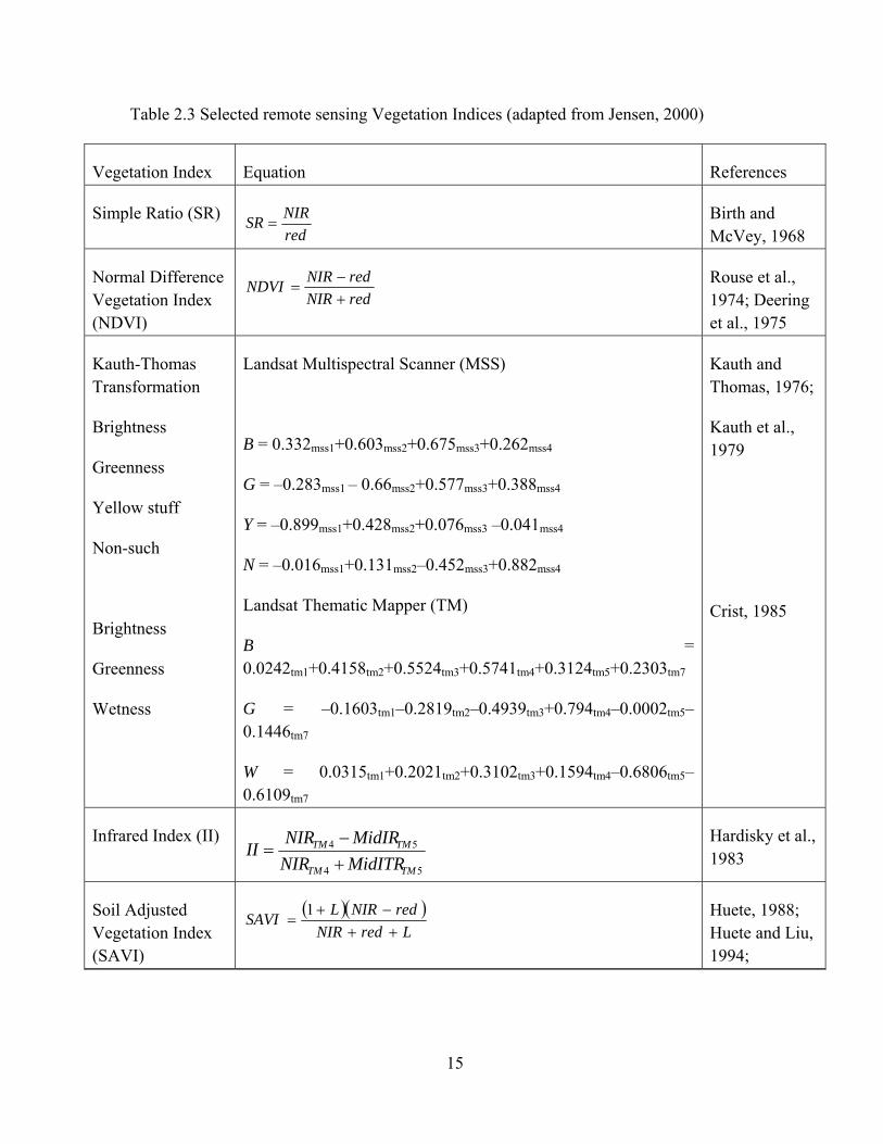
Table 2.3 Selected remote sensing Vegetation Indices (adapted from Jensen, 2000)
Vegetation Index Equation References
Simple Ratio (SR) red
NIRSR
Birth and McVey, 1968
Normal Difference Vegetation Index (NDVI)
redNIR
redNIRNDVI
Rouse et al., 1974; Deering et al., 1975
Kauth-Thomas Transformation
Brightness
Greenness
Yellow stuff
Non-such
Brightness
Greenness
Wetness
Landsat Multispectral Scanner (MSS)
B = 0.332mss1+0.603mss2+0.675mss3+0.262mss4
G = –0.283mss1 – 0.66mss2+0.577mss3+0.388mss4
Y = –0.899mss1+0.428mss2+0.076mss3 –0.041mss4
N = –0.016mss1+0.131mss2–0.452mss3+0.882mss4
Landsat Thematic Mapper (TM)
B = 0.0242tm1+0.4158tm2+0.5524tm3+0.5741tm4+0.3124tm5+0.2303tm7
G = –0.1603tm1–0.2819tm2–0.4939tm3+0.794tm4–0.0002tm5–0.1446tm7
W = 0.0315tm1+0.2021tm2+0.3102tm3+0.1594tm4–0.6806tm5–0.6109tm7
Kauth and Thomas, 1976;
Kauth et al., 1979
Crist, 1985
Infrared Index (II)
54
54
TMTM
TMTM
MidITRNIR
MidIRNIRII
Hardisky et al., 1983
Soil Adjusted Vegetation Index (SAVI)
LredNIR
redNIRLSAVI
1
Huete, 1988; Huete and Liu, 1994;

16
Table 2.3 (cont).
Atmospherically Resistant Vegetation Index (ARVI)
rbnir
rbnir
pp
ppARVI
**
**
Kaufman and Tanre, 1992;
Huete and Liu, 1994
Soil and Atmospherically Resistant Vegetation Index (SARVI)
Lpp
ppSARVI
rbnir
rbnir
**
**
Huete and Liu, 1994;
Running et al., 1994
Enhanced Vegetation Index (EVI)
LLpCpCp
ppEVI
bluerednir
rednir
1
***
**
21
Huete and Justive, 1999
2.4.2 TM Tasseled cap
By analyzing the spectral development of crops over the growing season, Kauth and
Thomas (1976) considered the soil spectral as well and recognized that all other four spectral
channels data contain useful information. The original conceptual model for this was called
“tasseled cap”. While statistically rotating the data space into physically meaningful set,
Thomas (1976) explored the idea of brightness and greenness. With the launch of Landsat,
the model called “TM-Tasseled cap” – a series of indices (brightness, greenness and wetness)
was derived.
Brightness and Greenness were reformulated to account for new sensor
characteristics, and wetness was designed to contrast the SWIR bands against the visible and
NIR bands to express the water content of soils (Crist and Cicone, 1984). The Tasseled Cap
transformation is a global vegetation index. It could be used anywhere to disaggregate the

17
amount of soil brightness, vegetation and moisture content in individual pixel in Landsat
MSS and TM image.
2.4.3 Principal component transform
Principal components transformation (PCT) is suggested for efficient hyper-spectral
remote-sensing image classification and display. The advantage of using a PCT is that global
statistics are used to determine the transformation parameters. The multispectral nature of
remote sensing image data can be contained by constructing a vector space with as many
axes as there are spectral components associated with each pixel. With Landsat Thematic
Mapper data, it will have six dimensions. The first principal component image will be
expected to contain 95% of the data variance. The variance in the last component is seen to
be minor and this component will appear almost totally as noise of low amplitude. An
application of principal components analysis is in the change detection with time between
images of the same region (Richards and Jia, 2006).
2.5 Applications of NDVI
The time series analysis of seasonal NDVI data has provided a method of monitoring
phonological patterns of the Earth’s vegetated surface. Chang (2007) monitored and mapped
corn and soybean in the United States using 500-m MODIS NDVI time series data. Brian and
Stephen (2005) used 250-m MODIS NDVI data to build state level crop maps in the US
Central Great Plains and demonstrated that time-series MODIS 250m NDVI is a possible
option for accurate and detail regional-scale crop mapping in the US Central Great Plains
with relatively high accuracies (> 84%). Jianqiang et al., (2006) used MODIS_NDVI data for
Shandong, China to estimate regional winter wheat yield.

18
Landsat TM/ATM+ data with multiple spectral bands and 30 m resolution have
proven useful for watershed–scale crop mapping (Van Niel et al., 2005; Mosiman, 2003).
The LULC maps derived from Landsat TM and ETM+ data, such as United States
Geological Survey’s (USGS) National Land Cover Dataset (NLCD) (Homer et al., 2004) and
Gap Analysis Program (GAP) datasets (Wardlow et al., 2006) have classified cropland area
into a single or limited number of thematic classes and are infrequently updated. The United
State Department of Agriculture (USDA) National Agricultural Statistic Service (NASS) 30
m crop land data layer (CDL) is detailed and annually updated (Craig 2001). However, the
production of LULC datasets from CDL in previous years was limited to a number of
selected portions of the US and the methodology to create CDL maps of NASS based solely
on their detailed annual sampling data are not available outside the agency. Landsat
TM/ETM+ data for local land cover classification has been demonstrated (Collingwood,
2008). However, data availability and quality issues (cloud cover) associated with acquiring
imagery at optimal times (growing season) are a factor (DeFries and Belward, 2000) due to
their limited temporal resolution. Coarse resolution, time series MODIS NDVI data are
useful for land cover classification for regional/national scale up to the global scale
(Wardlow et al., 2007; Zhang et al., 2003). The method used in this research was
unsupervised classification of multiple Landsat TM images and identified classes based on
MODIS-derived NDVI trends for selected crop types in the watershed area, including winter
wheat (winter crop), corn, soybean, grain sorghum (summer crops) and grassland - both hay
and pasture to support beef cattle production and as Conservation Reserve Program (Lerch et
al., 2008)
19
Based on NDVI values over a growing season in NDVI-time coordination, a crop
growth dynamic useful for the classifying process was achieved. This profile shows the
variation of NDVI of crop from plant to harvest. Each crop type has a unique, well defined
multi-temporal NDVI profile. These profiles should reflect unique phenological
characteristics of crop types.
2.6 GIS and Remote Sensing Software
A geographic information system (GIS) is a set of tools used to capture, store,
analyze, manage, and present data that are linked to locations. GIS can be used as a merging
of cartography, statistical analysis and database technology. Remote Sensing software is
Image Processing software for reading, processing, analyzing and displaying information
from digital geospatial imagery.
There are several GIS and Remote Sensing software used nowadays. In this study,
three programs were used: ERDAS IMAGINE 9.1, ENVI 4.7 and ArcGIS 9.3. ERDAS
IMAGINE was used most in this study to treat and analyze Landsat data. Model maker tool
in ERDAS was used to integrate raster spatial analysis and design new image processing
techniques. Unsupervised and IMAGINE Expert Classifier were used to build and perform
geographic expert system for image classification and post classification.
ENVI was used most of the time with MODIS NDVI data and to assess and analyze
MODIS NDVI profile for each type of crops. Also the SPEAR tool in ENVI was useful to
link between observed areas with Google Earth Image, which is a good source for
Geocorrection and Geo reference. ArcGIS was used to build the research area boundary from

20
NASS county boundary and to build sample points from field data to use in accuracy
assessment process.

21
Chapter 3
METHODOLOGY
3.1 Study site
The Salt River basin (Figure 3.1) is located in northeastern Missouri. River and
stream flow from the Upper Salt River drains into Mark Twain Lake since the closing of
Clarence Cannon Dam in 1983. Mark Twain Lake, a 7533 hectare reservoir with a shoreline
of 460 kilometers, is the source of drinking water for approximately 42,000 people in the
area. About 6000 km2 of total watershed area drains into the four streams: the North Fork
(26%), South Fork (14%), Middle Fork (14%) and Elk Fork (12%) (Allen, 2000). The other
five sub-basins in the area are Long Branch (8%), Lick Creek (6%), Crooked Creek (5%),
Otter Creek (5%), Black Creek and several small streams (10%). The South Fork sub-basin,
which begins in Audrain and Boone counties, and the Lick Fork sub-basin, which begins in
Audrain, drain northward to Mark Twain Lake. Elk Fork begins in Randolph and drains
eastward to Mark Twain Lake. Both the Middle Fork, which begins at Adair-Macon county,
and the North Fork, which begins at Schuyler county, drain southeastward to Mark Twain
Lake. Two major soils in the drainage area are the Putman-Mexico and Mexico-Leonard-
Armstrong-Lindley (SCS 1974-Ralls county; 1979-Knox, Monroe and Shelby counties,
1989-Randolph County), both which are characterized by moderate to high clay content.
Landform is classified as: 16 percent upland (0-3 percent gradient); 45 percent gentle slopes
(3-10 percent gradient); 21 percent steep slopes (>10 percent gradient) and 18 percent
floodplains (0-3 percent gradient). Only the areas near streams and river, and steeply sloping
sites were originally forested. Agriculture accounts for 77 percent of land in the basin (Lerch
et al., 2008). Land cover types of five major sub-basins in the watershed are given in Table

22
3.1. Corn, soybean and wheat are the predominant crops grown in the basin (SCS 1974,
1979, 1989). Characterized by clay pan soils, which are especially susceptible to soil erosion,
and gentle slope, the watershed results in a high runoff potential. Finney (1986) estimated
that 95 percent of sediment supplied to Mark Twain Lake would be trapped in the reservoir.
Suspended matter deposited in reservoirs reduces their storage capacity and their ability to
control flooding (Choubey and Subramanian, 1992). Sediment affects water quality and its
sustainability for drinking water, recreational and industrial uses (Lodhi et al., 1997).
Because of the documented soil and problems of herbicide and sediment in surface water,
water quality and flow monitoring were initiated basin-wide in 2005 and the Salt River basin
was selected as one of twelve USDA Agricultural Research Service (ARS) benchmark
watersheds for the Conservation Effects Assessment Project (CEAP) (Lerch et al., 2008).
Besides monitoring surface runoff flow and sample water quality in streams, a regional land
use and geology land classification were required to develop a cropping system to improve
watershed management.
Table 3.1 Gradients, basin area and percentages of cover types in the Upper Salt River Basin in 1990 (Skadeland, 1992)
Percent Land Cover Types
Stream Area (ha) Gradient Crop Grass Forest Other
Major inflows to Mark Twain Lake:
Lick 24,179 0.18 70 16 12 2
Elk 57,794 0.18 52 25 18 5
South 76,748 0.17 56 21 18 5
Middle 91,421 0.12 41 32 21 6
North 116,397 0.11 51 28 12 9

23
Figure 3.1 Salt River Basin (Lerch et al., 2008)
3.1.1 Summer crops
Summer crops planted in the area are corn, soybean and grain sorghum. Although
these summer crops have similar crop calendars, each has a unique spectral-temporal
response and different appear among crops. Summer crops have their growth cycles occur
during summer, with mid-summer peak NDVI values (peak greenness). The timing and
amount of rainfall and the heat and dryness are two weather factors that affect summer crop
growth stage and greenness. The USDA NASS has the information about initial planting date
for corn, soybean, and sorghum for Missouri.

24
Figure 3.2 Corn Growth Stage Development (Source: http://weedsoft.unl.edu/documents/GrowthStagesModule/Corn/Corn.html#)
Corn growth stage is shown in Figure 3.2. Corn is planted after snow is gone and the
soil is thawed. Typical corn plants develop 20-21 total leaves, silk about 65 days after
emergence and mature around 125 days after emergence. Corn is the earliest planted summer
crop (initial planting date is mid-April and to early June). Corn had the earliest green up,
between June 10 and June 26. Corn NDVI peaked in the watershed area during the August 13
period with the NDVI value about 0.77 and higher (Wardlow et al., 2007). Mid-September
until mid-October represents the senescence phase of corn, which shows the large NDVI
decrease on the NDVI profile.
25
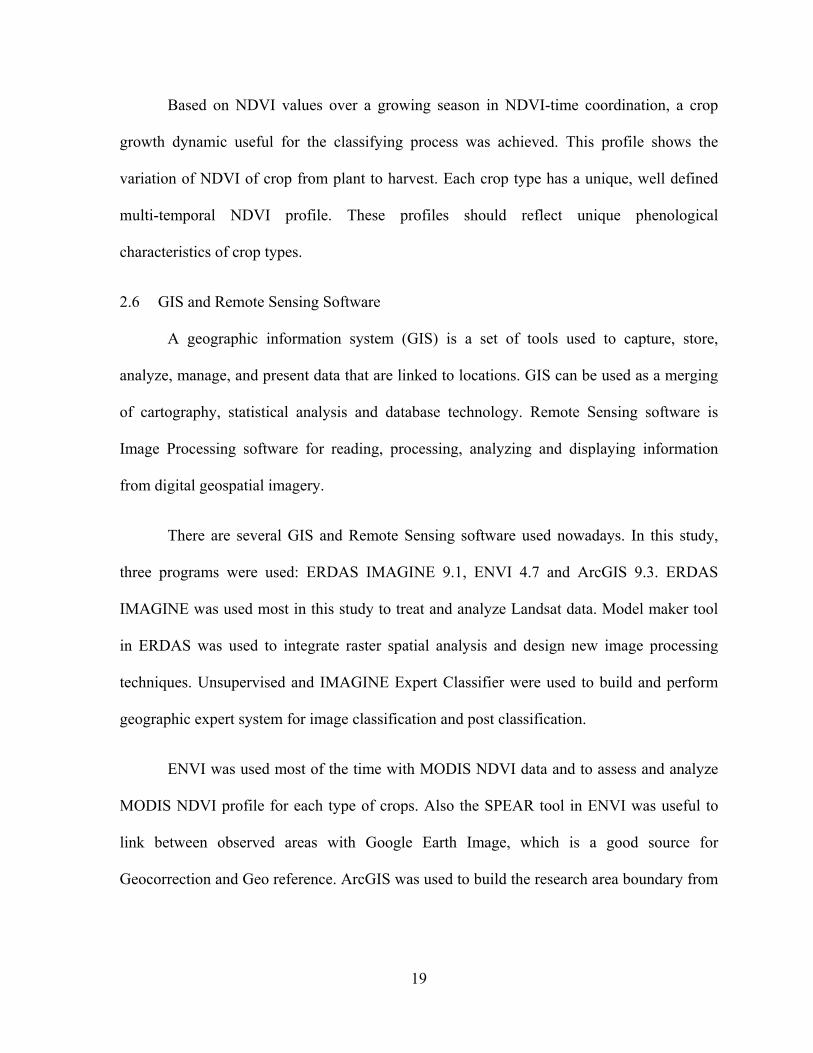
Figure 3.3 Soybean Growth Stage Development (Source: http://weedsoft.unl.edu/documents/GrowthStagesModule/Soybean/Soy.html#)
Soybean Growth Stage is shown in Figure 3.3. Soybean has a wide range of planting
dates, but is typically after corn. May 1 to Jun 10 is the normal period to plant soybean.
Planting later in June could result in a loss of soybean yield. Double crop (soybean planted
after harvesting small grain) in northern Missouri may result in failure because of a shorter
growing season (Harry and William, 1949). Double cropping in the Salt River basin area is
more successful when there is sufficient soil moisture immediately after the small grain
harvest. Soybean green up period is about July 12. Peak greenness of soybean is around
August 29 with an NDVI value about 0.84 and higher (Wardlow et al., 2007). Soybean
maintains a high NDVI until late-September and has a rapid NDVI decrease in mid-October,
representing the senescence phase of soybean (Rogers, 1997).
26
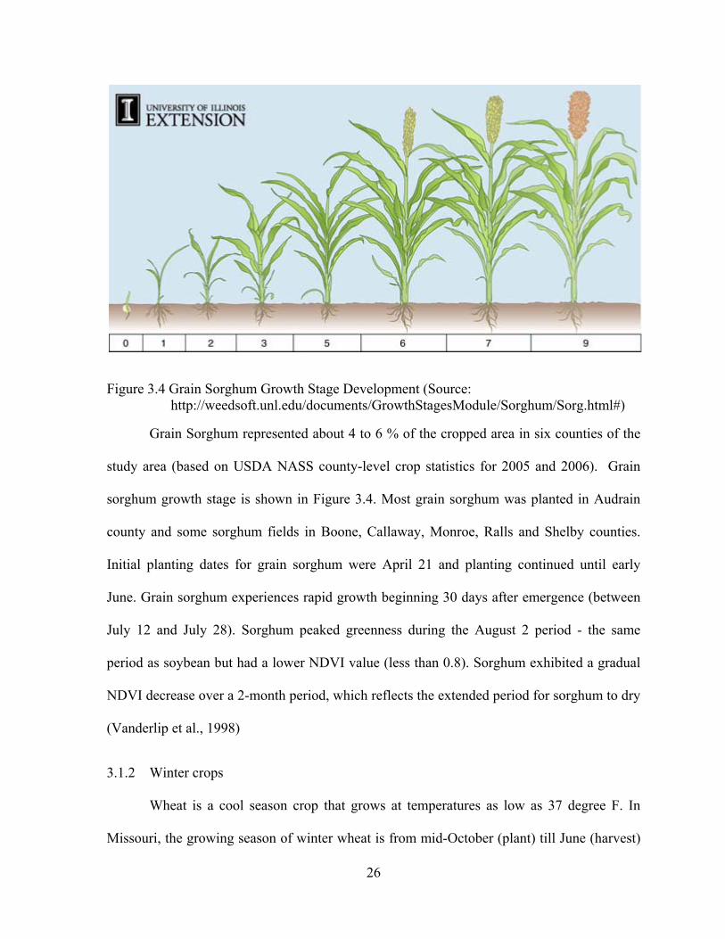
Figure 3.4 Grain Sorghum Growth Stage Development (Source: http://weedsoft.unl.edu/documents/GrowthStagesModule/Sorghum/Sorg.html#)
Grain Sorghum represented about 4 to 6 % of the cropped area in six counties of the
study area (based on USDA NASS county-level crop statistics for 2005 and 2006). Grain
sorghum growth stage is shown in Figure 3.4. Most grain sorghum was planted in Audrain
county and some sorghum fields in Boone, Callaway, Monroe, Ralls and Shelby counties.
Initial planting dates for grain sorghum were April 21 and planting continued until early
June. Grain sorghum experiences rapid growth beginning 30 days after emergence (between
July 12 and July 28). Sorghum peaked greenness during the August 2 period - the same
period as soybean but had a lower NDVI value (less than 0.8). Sorghum exhibited a gradual
NDVI decrease over a 2-month period, which reflects the extended period for sorghum to dry
(Vanderlip et al., 1998)
3.1.2 Winter crops
Wheat is a cool season crop that grows at temperatures as low as 37 degree F. In
Missouri, the growing season of winter wheat is from mid-October (plant) till June (harvest)

27
of the next year. There are three highlight points on the winter wheat NDVI profile. Start-up
point begins with low NDVI from January through April. Winter wheat greens up rapidly
from mid-April. Since other crops are just germinating, it is easy to distinguish winter wheat
from the other grains. Peak point occurs in late May until early June, followed by the rapid
decrease of NDVI due to wheat’s senescence and harvest. Then “valley” point appears after
wheat harvests, followed by a second peak resulting from grass and weeds or soybean (if the
condition was possible for double cropping). Wheat growth stage is shown in Figure 3.5.
Figure 3.5 Winter Wheat Growth Stage Development (Source: htttp://weedsoft.unl.edu/documents/GowthStagesModule/Wheat/Wheat.html#)
3.1.3 Grass/Pasture hay
Grass/Pasture hay NDVI profile has a characteristic of grass’ phenology of “growth
and cut” cycle. Grass/pasture hay begins growth in mid April, represented by a rapid NDVI
increase from 0.38 to greater than 0.7. After that, grass, which used as hay, was followed by
two or three times of decreasing (cut) and increasing (growth) of NDVI during the summer.

28
The gradual decrease of NDVI from late October until December matches the senescence of
grass/hay.
3.1.4 Other features
Fallow is the practice of leaving the idle field as a dry-land farming technique to
conserve soil moisture for the following year (Havlin et al., 1995) resulting in a low NDVI
during growing season. Full year fallow is not applied in wet region as Missouri. Short time
fallow is applied in several months after wheat is harvested.
Forest, which has high NDVI during the summer, can be separated from cropland by
rapid NDVI increase in early summer, remaining high until mid-October with a gradual
decrease of NDVI. Water has low NDVI during the entire year, with a slightly NDVI
increase in summer due to turbidity of the water body. Urban/developing areas have a low
NDVI value and remain almost the same throughout the year.
3.2 Materials
Landsat Thematic Mapper (TM) images for the growing seasons in year 2005 and
2006 were obtained. Due to lack of cloud free imagery, there were only four images for
2005: May 23, June 24, July 10 and Oct 14 and three images for 2006: Apr 8, Sep 15 and Oct
01. A complete image for the study area was created by mosaic Landsat Row 32 Path 25 and
Landsat Row 33 Path 25 (Figure 3.6). The complete image from Landsat TM was a layer
stack of 6 bands. Landsat TM images were at level 1 geometrically corrected, meaning that it
was provided systematic radiometric and geometric accuracy. The scene had been rotated,
aligned, and georeferenced to UTM map projection.
29
The 16-day composite 250m resolution MODIS Terra NDVI product was acquired
through NASA-DAAC EROS Data Center. The upper part of the watershed area was in
h10v4, which was in zone 13 and the lower part of the watershed was located in h10v5,
which was in zone 15. There were three kinds of errors associated with MODIS data product
beside cloud cover – geo-referencing, atmospheric correction and bidirectional reflectance
distribution function (BRDF) effect. Errors in reflectance are partly reduced with NDVI. In
order to reduce this effect, Doraiswamy et al. (2006) used multiple steps in the Savizky-
Golay filtering method to smooth every pixel’s time series profile through the entire year.
The area of interest (AOI) used to subset the study from remote sensing data is the
county-boundary of 11 counties where the Salt River basin is located (Figure 3.6 and 3.7)
The county boundary is available on CARES - Center for Agriculture, Research and
Environmental Studies. The Farm Facts in Missouri reported by USDA NASS for 2005 and
2006 was obtained to analyze relationship between weather and crops NDVI.
3.2.1 Reference data
Ground truth data were obtained from USDA NASS CDL map for Missouri in year
2006 (Figure 3.8). Reference data were also collected from field observations in year 2005
and 2006 at two reference areas: Goodwater Creek and Greenley, MO. These two data sets
were used for accuracy assessment of 2 maps. Results were also compared to county-level
crop statistics (USDA NASS) (Table 3.2 through 3.4).

30
Figure 3.6 (a) A mosaic of Landsat TM row 32 and 33 path 25 (23 May 2005) and (b) Salt River Basin county-boundary.

31
Figure 3.7 False color Landsat image for 23 May 2005 subset to the county boundary of Salt River Basin.

32
Table 3.2 USDA NASS county statistics (2000)
Water (mi2) Land (mi2) Total (acres)
Adair 2.313 567.005 362883.2
Audrain 3.692 693.096 443581.4
Boone 5.881 685.43 438675.2
Callaway 8.194 838.836 536855
Knox 1.067 505.774 323652.5
Macon 8.762 803.769 514412.2
Monroe 24.244 645.982 413428.5
Ralls 12.819 470.998 301438.7
Randolph 5.331 482.319 308684.2
Schuyler 0.288 307.868 197035.5
Shelby 1.495 500.935 320598.4
Total (11 counties) 74.086 6502.012 4161245
Table 3.3 USDA NASS county-level crop statistics for 2005 (acres)
Corn
harvested
Sorghum
harvested
Soybean
harvested
Wheat
harvested
Hay
harvested
Adair 14000 x 38800 1400 50000
Audrain 72100 20000 157400 11400 24000
Boone 24100 3600 43500 4300 37000
Callaway 19800 4000 59400 6600 46000
Knox 40200 x 75800 1600 27000
Macon 24700 x 73000 6000 54000
Monroe 48300 4700 74600 2900 31000
Ralls 46800 3900 74700 6600 18000
Randolph 15300 1100 44100 4400 35000
Schuyler 8500 x 18200 x 29000
Shelby 42800 4100 93500 6100 25000

33
Table 3.4 USDA NASS county-level crop statistics for 2006 (acres)
Corn
harvested
Sorghum
harvested
Soybean
harvested
Wheat
harvested
Hay
harvested
Adair 11900 x 38200 3700 51000
Audrain 67200 15000 168000 24400 26000
Boone 19300 2500 46300 9500 38000
Callaway 19500 3500 61500 10400 53000
Knox 34800 x 71700 7600 27000
Macon 20400 x 75200 10700 49000
Monroe 42600 3000 77300 12800 34000
Ralls 42700 2500 79500 14200 21000
Randolph 13800 x 43000 9500 40000
Schuyler 6400 x 18500 900 29000
Shelby 37700 3400 98400 11500 29000

34
Figure 3.8 USDA NASS CDL map subset to the Salt River Basin (2006).

35
3.3 Image Preprocessing
The coordinate of Landsat images were adjusted to match the mosaic USGS DOQQ
image (from CARES) for the study area. The images after adjustment were also checked with
Google Earth using the SPEAR application in ENVI at points as intersection of highway on
image.
Song et al. (2001) stated that no atmospheric correction is required if the
classification was done based on multiple date composite imagery composited if all of them
were rectified and in a single dataset. Kawata et al. (1990) also stated that atmospheric
correction has little effect on classification accuracy, as long as the training data and the
image are on the same relative scale. Since in this study, the author used all the images used
for classification from Landsat 5 TM for multiple dates at the same place, no the atmospheric
correction was applied.
A NDVI image derived from Landsat TM data band 3 (Red) and band 4 (near IR)
with the equation
34
34
BandBand
BandBandNDVI
(3.1)
NDVI is a unitless index and the NDVI data derived from Landsat TM is expressed in
number of ranges -1 to 1.
In addition to 6 bands from Landsat TM and NDVI data derived from Landsat, three
other components were used: brightness, greenness and wetness. Tasseled cap values for the
Landsat 5 TM were generated using the application in ERDAS Imagine.

36
The MODIS images (zones 13 and 15) were clipped into smaller portions to re-
project to the same zone and then were re-projected from ISIN projection to UTM using
ENVI. The ERDAS Imagine was then used to subset the imagery using AOI (area of interest)
as the boundary of the eleven counties in the Salt River basin. After that, a twenty-three 16
days 250m NDVI product was built by layer stacking 23 MODIS NDVI images (for a whole
year). A small model was built in ERDAS to smooth the NDVI curves for each pixel in the
image using a 2nd order polynomial and 7 point Savitzky-Golay filter. The equation for this
particular Savitzky-Golay smoothing is defined as follows:
21
2367632 321123 ttttttt
t
xxxxxxxy (3.2)
Figure 3.9 shows the smoothing results.
3.4 Previous crop discrimination study on the Salt River watershed
Jang et al. (2009) conducted a previous study done on the Salt River watershed to
create a crop type classification map for 2003 from five dates in the growing season: 26 May,
5 July, 22 August, 7 September, and 23 September. Jang et al. (2009) evaluated and
compared two different crop type classification methods using data from the 2003 crop year.
The first method used unsupervised classification of multiple Landsat images, followed by
manual class identification using ground survey data. The second method also used
unsupervised classification of multiple Landsat images, followed by class identification using
MODIS-derived seasonal NDVI trends. Jang et al. (2009) concluded that the second method
improved the overall accuracy of the crop type map to 86%, compared with an 83% accuracy
from method one. They concluded that method two can provide better results with less
training data. In creating the 2003 crop classification map, Jang et al. (2009) resampled 250-

37
m resolution MODIS images to the 30-m resolution of the Landsat image. They combined
five Landsat images to make a 30-band composite image and unsupervised this combined
image to 150 clusters. They extracted the pixels in the stack of MODIS NDVI images
corresponding to each of the 150 clusters and imported them into SAS. The tree procedure
was done in SAS to group the 150 classes based on their mean MODIS-derived NDVI trends.
Figure 3.9 The 23-band NDVI trend curve of sample pixel before and after smoothing (extract from ENVI through 2-profile spectral curve).

38
In this research, the author also used a decision tree and analyzed MODIS-derived
NDVI trends to create crop classification maps for the Salt River Basin in 2005 and 2006, but
because of the lack of cloud-free Landsat images in the growing season, it was impossible to
extract the NDVI trends. In the combination of the three Landsat images in 2006 (April,
September and October), trends were similar among summer crops and also similar to grass
and forest – with the same green up stage in April and senescence stage in September and
October. In the combination of Landsat images in 2005, it would be useful to separate
winter wheat and grass from summer crops but there was still a difficulty in discriminate
summer crop trends, especially soybean and grain sorghum.
The author chose not to resample 250-m resolution MODIS image because it would
provide numerous mixed pixels and be impossible to extract the necessary data such as
maximum NDVI, minimum NDVI, date of maximum NDVI, etc. The 23-band MODIS
NDVI image was still created to extract the NDVI profile (ENVI z-spectral profile) for each
crop type. Crop NDVI profile was then analyzed using the USDA weather report to
determine the threshold applied in the decision tree. In this study, the author used
unsupervised classification each of Landsat image obtained and create an NDVI map from
each Landsat image. The decision tree used in this study was a combination of analyzing
pixel NDVI and its possible unsupervised class at each point in time. Principal components
transformation and Tasseled cap were also applied in decision tree to get better result.
3.5 Image Processing
In this study, classification was done based on the combination of unsupervised
classification (pixel-based) and a decision tree (object-based). The ISODATA method of
unsupervised classification was applied using a 0.995 convergence threshold and run with ten

39
iterations to cluster each Landsat image into 150 clusters. This process was done with
ERDAS Imagery. The NDVI profile for each object class in the watershed, such as water,
urban, grass, forest, corn, soybean, etc, was examined using ENVI z-spectral profile. Based
on the phenological profile of each type, hypotheses were established for creating a decision
tree. Unsupervised classification methods have overall good results for agricultural areas
(Cohen and Shoshany, 2002), together with object-based methods, which divide the satellite
image into objects or segments that represent a homogenous unit on ground, as a way to
improve accuracy (Aplin and Atkinson, 2001; Walter, 2004).
3.5.1 Class Identification Process
All 150 clusters from unsupervised classification images were grouped and labeled
into nine land cover classes: water, forest, urban, grass/hay, double cropland, winter wheat,
corn, soybean and sorghum using ERDAS Imagery using the Knowledge Classifier
procedure. All pixels from image were grouped based on its NDVI value for each point of
time, spectral characteristics (USC classes) and brightness, greenness and wetness.
Knowledge Engineer, an ERDAS Imagery decision tree procedure, known as expert
classification, provides a rules-based approach to image classification, post-classification
refinement. It is a hierarchy of rules, or decision tree. A rule is a conditional statement or list
of conditional statements about an object’s attributes that determine a hypothesis.

40
Chapter 4
RESULTS AND DISCUSSION
4.1 Analysis
4.1.1 Analysis of Landsat data in 2006
Landsat 2006 cloud free data were obtained April 8, September 15 and October 01 ,
which are shown as red, green and blue lines in MODIS NDVI profiles (Figure 4.1 to 4.6).
From the Weather Review Report from NASS for Missouri in year 2006, wet March
followed by dry April pushed wheat maturation ahead of normal. Wheat NDVI values had
not yet reached the peak greenness in April but were high and close to peak in late May with
NDVI value greater than 0.6 (Figure 4.1). Most of April was dry which allowed rapid
planting of row crops, but NDVI values for these summer crops were still low (less than 0.4)
(Figure 4.2 to 4.4). Grass and forest were greening up at the time the April Landsat image
was obtained, with a NDVI greater than 0.5 but still less than winter wheat (Figure 4.5 and
4.6).
At the time the second and third Landsat images were obtained on September 15 and
October 01, the corn harvest was already finished. Heat and drought in the first part of
August stressed the pasture and row crops. By August 27, Farm Fact reported that 90% of
corn was in the dent stage with harvest to soon follow. In early to mid September, soybean
and sorghum were just passed peak greenness and maintained a high NDVI value. Sorghum
began senescence with onset of dry weather, while soybean still had a high NDVI value
(Figure 4.3 and 4.4). Dry and sunny weather over the first half of October made for a good
harvest condition. Soybeans had a rapid NDVI decrease in October but sorghum had a more

41
gradual decrease in the NDVI curve. The forest area kept a high NDVI value during the
observed period (Figure 4.5). Grass had cutting and re-growth NDVI curves (Figure 4.5) but
due to cloud cover during much of the satellite sampling periods, the NDVI trends of
grass/hay through three points of time had some characteristics similar to soybean and
sorghum.
Corn exhibited low NDVI in these three points of time, since in April it was just
planted, and by September, it was already in the dent stage and with harvesting completed by
the end of September (Figure 4.2). The rapid decrease of NDVI from mid September to early
October helped to discriminate soybeans from other crops (Figure 4.3). Mixed pixels
appeared at the boundary of fields, which had some characteristics similar to sorghum
(gradual drop of NDVI). Therefore, other components were applied to better classify
sorghum, soybean and grass/hay. These differences among vegetation types were applied to
build the hypotheses in the decision tree.
4.1.2 Analysis of Landsat data in 2005
Landsat 2005 cloud free data were obtained May 23, June 24, July 10 and October 14.
May 23, June 24 and July 10 were the three images during the growth season of summer
crops. The October 14 image was in late fall, when all summer crops were already in the
senescence stages but since there was lack of cloud free images in the growth season to
classify between summer crops, it was useful in providing additional information to better
discriminate between corn, soybean and grain sorghum.
The Weather Review Report from NASS for Missouri in 2005 indicated that by the
end of April, 72% of corn was in the ground but light frost in late April burned the upper

42
leaves. Wheat was processing well, mostly in fair to good condition. A dry cool May slowed
the growth of crops. During the third week of May, corn planting reached 98 percent. By the
end of May, 85 % of soybean and 90 % of grain sorghum were planted. The May 23 Landsat
image coincided with winter wheat reaching its greatest NDVI value. Grass and forest also
had a high NDVI value. Rain in early June improved summer crop growth. The wheat
harvest began the second week of June with 83 % of winter wheat harvested by the end of
June. The Landsat June 24 image showed the low NDVI condition of winter wheat fields and
increased NDVI value of other summer crops. Comparing NDVI values from Landsat images
of May 23 and June 24 revealed the information to separate winter wheat from other crops.
But extra information was needed to classify winter wheat and hay since hay harvest in June
also reduced its NDVI value.
Drought conditions were during mid August and the peak NDVI of soybeans and
sorghum were in late August (Figure 4.3 and 4.4). The ideal time to separate classes between
summer crops was during August and early September, when corn was harvested, grain
sorghum was in senescence but soybean maintained a greater NDVI value. Unfortunately, no
cloud-free Landsat image was obtained in that time. In October, a few periods of showers
slowed fall harvest. By the end of October, 93 % of corn was out of the field, 83 % of
soybean and 86 % of grain sorghum were harvested. Due to the fact that soybean NDVI
drops more rapidly than grain sorghum, the October 14 Landsat image was useful in
identifying each since soybean had a lower NDVI compared with grain sorghum. Analyzing
NDVI differences between July and October also assisted in classifying soybean and grain
sorghum.

43
Besides analyzing the NDVI value of vegetation, the information from Principal
Components and Tasseled Cap were also valuable in identifying differences over time. For
example, in June, when wheat was harvested, the NDVI of wheat was as low as grass. But
wheat fields had a greater brightness than grass. Tasseled Cap brightness was used to classify
urban/soil/fallow from vegetation. Tasseled Cap wetness was used to better separate water
bodies and wetland from other features.
4.1.3 Crop NDVI profiles
Crop NDVI profiles were obtained from MODIS 2006 data in Salt River Basin
watershed. The red line (left vertical line Fig. 4.1 to 4.6) is at the 7th band, the blue line (right
vertical line) is at the 18th band and the green line (middle vertical line) is at the 17th band in
a 23-day MODIS NDVI trend curve. The combination of these three bands (bands 7, 17 and
18) as red, green, blue match with the combination of three Landsat NDVI images obtained
in 2006.

44
Figure 4.1 MODIS Winter Wheat NDVI profile in 2006.
Figure 4.2 MODIS Corn NDVI profile in 2006.

45
Figure 4.3 MODIS Soybean NDVI profile in 2006.
Figure 4.4 MODIS Sorghum NDVI profile in 2006.

46
Figure 4.5 MODIS Forest NDVI profile in 2006.
Figure 4.6 MODIS Grass NDVI profile in 2006.

47
4.2 Decision tree rules
The decision tree was built using the Knowledge Engineer Module in Erdas Imagine.
This program provides a graphical user interface for the "expert" to build a tree diagram
consisting of final and intermediate class definitions (hypotheses), rules (conditional
statements concerning variables), and variables (raster, vector, or scalar). Hypotheses are
evaluated by the use of rules – if one or more rules are correct, then that hypothesis may be
true at that particular location. The rule is evaluated based on input variables in order to
determine if a rule is true. Variables could be in the form of an existing image or it could
even be an external program. Variables can also be defined from vectors and scalars. If the
variable’s value indicates that the rule is correct and all the rules defined the hypothesis is
correct, the hypothesis (class allocation) is true. Decision trees are shown in Appendix A.
4.2.1 Decision rules to separate water and urban/soil from the others
Both water and urban/soil have a low NDVI value at any point of time, but water
bodies show as a black feature in the Landsat image while urban/soil has a bright color in the
Landsat image. Applying this analysis, pixels of water would have a low NDVI and USC
class less than 20 (black feature), while pixels of urban/soil would be low in NDVI and USC
greater than 20.
Soil/fallow pixels would be classified as urban/soil if the area was limited to weeds,
but it would be classified as grass if there was an abundance of weeds in idle cropland.
Figure 4.7 is as example of decision tree diagram to classify water.

48
Figure 4.7 Decision rules to define water for 2005
where
o Testing hypothesis: Water o NDVI_1, NDVI_2, NDVI_3, NDVI_4: NDVI value extracted from Landsat NDVI
2005 images for May 23, June 24, July 10 and October 14 respectively. o USC_3: unsupervised classification cluster of Landsat TM for June 24, 2005
Explanation of decision tree process for water identification:
If (NDVI_1 ≤ 0.02 and USC_3 ≤ 20) or (NDVI_2 ≤ 0.02 and USC_3 ≤ 20) or
(NDVI_3 ≤ 0.02 and USC_3 ≤ 20) or (NDVI_4 ≤ 0.02 and USC_3 ≤ 20)
Then (Water = true) End if.
4.2.2 Decision rules to separate winter wheat and double crop from the other land uses
Winter wheat has a higher NDVI than other objects in April and May. Winter wheat
NDVI could reach 0.45 in April and higher in May (>0.5) while summer crop NDVI remains
low. Grass has the same green up stage in April and May, which has an NDVI of 0.45 or
greater. Wheat could be separated from grass if there were data in June and July, which

49
indicates the cutting and regrowth of grass/hay. Winter wheat – fallow shows high NDVI in
April and May (>0.5) but low NDVI in September and October (<0.4), which could partly
separate it from grass if grass shows the regrowth stage in September and October. Winter
wheat – soybean double crop exhibits a high NDVI value in April/May and a high NDVI
value in July/August as well. Again, double crop could be mis-classified as grass and vice
verse because they exhibit the same trends in April and September.
4.2.3 Decision rules to separate corn from the other summer crops
Corn was the earliest planted summer crop, so its NDVI in April was higher than the
other summer crops but less than grass and winter wheat. Corn has the highest NDVI value
among summer crops in July (since there was no August image obtained in 2005 and 2006)
with a NDVI value higher than 0.5 into September. Some corn was already harvested, and
exhibited a bare soil (bright feature) with USC in September greater than 145. Other corn
fields that had not yet been harvested had a low NDVI value similar to other summer crops,
but the corn harvest was done in late October, with USC in October greater than 130.
4.2.4 Decision rules to separate soybean and grain sorghum
These two summer crops are difficult to separate because they have the same initial
planting date and show the same trends during the growing season. During the growing
season, soybean always has a higher NDVI value than grain sorghum. The phenology of
these two crops in the senescence stage was applied. Soybean NDVI decreases rapidly while
grain sorghum has a gradual NDVI decrease. It was possible that grain sorghum NDVI in
July was less than the NDVI in September (NDVIJul – NDVISep < 0) due to high air
temperature in July and rainfall in August. If NDVI difference from September to October
was greater than 0.3, it would be classified as soybean. In 2006, some sorghum pixels had an

50
NDVI trend similar to grass/fallow, making it difficult to separate grass/fallow from
sorghum.
4.3 Accuracy assessment
One of the most common means to express accuracy of classification is the
preparation of a classification error matrix. An error matrix is based on category to category
comparison, the relationship between known data (reference ground truth data) and results
from automated classification. The error matrix expresses omission (exclude) error and
commission (include) error. The overall accuracy is also computed by dividing the total
number of correctly classified pixels by the total number of reference pixels. In addition, the
producer’s and user’s accuracies are also obtained from the error matrix. The producer’s
accuracies are the accuracies of individual categories, which are computed by dividing the
total number of correctly classified pixels in each category by the total number of pixels in
the corresponding column of matrix. User’s accuracy is calculated by dividing the number of
correctly classified pixels in each category by the total number of pixels in corresponding
row.
The k̂ (k_hat) statistic (Kappa analysis) was also obtained after the accuracy
assessment procedure in ERDAS. The k̂ is a measure of the difference between the actual
agreement between reference data and an automated classifier and the chance agreement
between the reference data and a random classifier. The k̂ statistic is computed as (Jensen,
2000)

51
r
iii
r
i
r
iiiii
xxN
xxxNk
1
2
1 1ˆ (4.1)
where
r = number of rows in the error matrix
xii = number of observations in row i and column i (on the major diagonal)
xi+ = total of observations in row i (shown as marginal total of right sideof the matrix)
x+i = total of observations in column i (shown as marginal total of bottom of the matrix)
N = total number of observations included in matrix
The overall accuracy only includes the data along the major diagonal and excludes
the errors of omission and commission The k̂ incorporates the nondiagonal elements of the
error matrix as a product of the last row and column.
Congalton (1991) recommended that a minimum of 50 sample points should be
obtained in each category. Since sorghum and wheat were planted in fewer fields than corn
and soybean, the number of sample points for each crop varied. The NASS CDL crop map
subset to watershed area was used for the accuracy assessment process for the 2006 crop
map. For the accuracy assessment for the 2005 crop map, an error matrix was prepared for
two reference areas (Goodwater creek sub-basin and Greenley reference area) where ground-
truth data were available. For the accuracy assessment for the 2006 crop map, an error matrix
was also prepared for two reference areas (Goodwater creek sub-basin and Greenley
reference area) where ground-truth data were available. Also, an error matrix was prepared
for the whole watershed area for comparison with NASS CDL map.

52
There were 308 points taken from 141 fields in the Goodwater creek sub-basin and
257 points taken from 168 fields in the Greenley reference area for accuracy assessment
process for the 2005 crop map. With the accuracy assessment process for the 2006 crop map,
488 points were taken from 224 fields in Goodwater creek sub-basin and 232 points were
taken from 198 fields in Greenley reference area. Sample points were chosen randomly using
2 or 3 points in small fields and more points in larger fields instead of one point per field in
order to reduce the chance of taking mixed pixel points.
For the 2006 crop map, the overall accuracy was 87.09% for Goodwater Creek sub-
basin (Table 4.4) and 96.98% for Greenley reference area (Table 4.3) compared with field
data in two areas, and overall accuracy for the whole watershed area was 94.08% when
compared with the NASS CDL map (Table 4.5). The accuracy of Goodwater Creek sub-
basin was lower than the Greenley reference area due to the fact that no grain sorghum was
planted in the northern part of the basin area. Due to the difference in resolution from the
study’s map (30 m resolution in Landsat image) and the CDL map (56 m resolution), there
were some pixels that were classified in different classes. For example, there were some
small ponds inside the urban area that could not be seen in the CDL 56 m resolution but were
identifiable with 30 m Landsat resolution. The CDL map was created based on NASS annual
survey data that can help to classify more classes than the map from this study, such as grass,
hay/pasture, red clover, alfalfa, and etc; and better classify grain sorghum with other crops.
There was no NASS CDL map to use for verifying the 2005 crop map. Accuracy
assessment was done with field data taken from the two reference areas in the area. The
overall accuracy was 92.53% for the Goodwater Creek sub-basin (Table 4.2) and 93% for the
Greenley reference area (Table 4.1). Again, the appearance of grain sorghum in the south

53
part of the area reduced the overall accuracy of the Goodwater creek sub-basin compared to
the Greenley reference area. The accuracy was higher in 2005 compared with the 2006 map
since more images were available during the growth season in 2005.
The Kappa coefficient for each accuracy assessment procedure was shown in Table
4.1 through 4.5. Additional statistical comparisons of both crop maps with crop area statistics
from NASS were done. Results are shown in Table 4.6 and 4.7
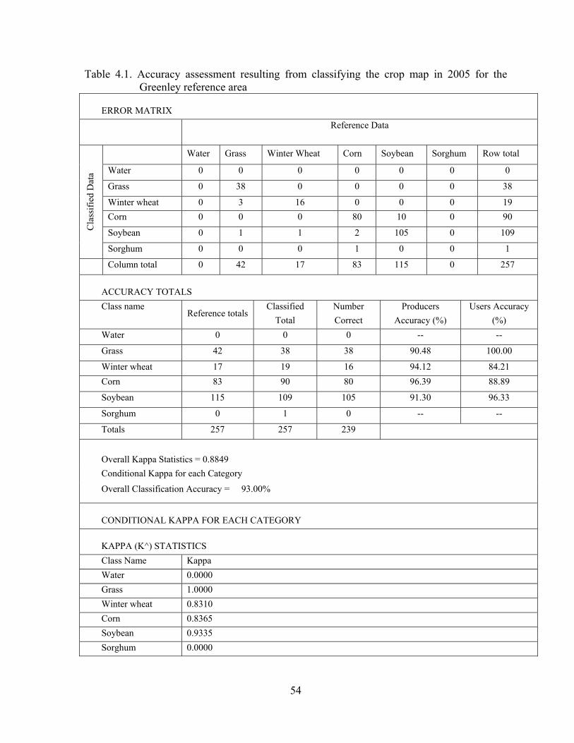
54
Table 4.1. Accuracy assessment resulting from classifying the crop map in 2005 for the Greenley reference area
ERROR MATRIX
Reference Data
Cla
ssif
ied
Dat
a
Water Grass Winter Wheat Corn Soybean Sorghum Row total
Water 0 0 0 0 0 0 0
Grass 0 38 0 0 0 0 38
Winter wheat 0 3 16 0 0 0 19
Corn 0 0 0 80 10 0 90
Soybean 0 1 1 2 105 0 109
Sorghum 0 0 0 1 0 0 1
Column total 0 42 17 83 115 0 257
ACCURACY TOTALS
Class name Reference totals
Classified
Total
Number
Correct
Producers
Accuracy (%)
Users Accuracy
(%)
Water 0 0 0 -- --
Grass 42 38 38 90.48 100.00
Winter wheat 17 19 16 94.12 84.21
Corn 83 90 80 96.39 88.89
Soybean 115 109 105 91.30 96.33
Sorghum 0 1 0 -- --
Totals 257 257 239
Overall Kappa Statistics = 0.8849
Conditional Kappa for each Category
Overall Classification Accuracy = 93.00%
CONDITIONAL KAPPA FOR EACH CATEGORY
KAPPA (K^) STATISTICS
Class Name Kappa
Water 0.0000
Grass 1.0000
Winter wheat 0.8310
Corn 0.8365
Soybean 0.9335
Sorghum 0.0000

55
Table 4.2 Accuracy assessment resulting from classifying the crop map in 2005 for the Goodwater creek sub-basin
ERROR MATRIX
Reference Data
Cla
ssif
ied
Dat
a
Water Grass Winter Wheat Corn Soybean Sorghum Row total
Water 8 0 0 0 0 0 8
Grass 0 30 1 0 0 0 31
Winter wheat 0 2 7 0 1 0 10
Corn 0 0 0 78 5 0 83
Soybean 0 0 0 4 136 6 146
Sorghum 0 2 0 0 2 26 30
Column total 8 34 8 82 144 32 308
ACCURACY TOTALS
Class name Reference
totals
Classified
Total Number Correct
Producers
Accuracy (%)
Users Accuracy
(%)
Water 8 8 8 100.00 100.00
Grass 34 31 30 88.23 96.77
Winter wheat 8 10 7 87.50 70.00
Corn 82 83 78 95.12 93.98
Soybean 144 146 136 94.44 93.15
Sorghum 32 30 26 81.25 86.67
Totals 308 308 285
Overall Classification Accuracy = 92.53% KAPPA (K^) STATISTICS
Overall Kappa Statistics = 0.8826
CONDITIONAL KAPPA FOR EACH CATEGORY
Class name Kappa Water 1.0000
Grass 0.9300
Winter wheat 0.6921
Corn 0.9177
Soybean 0.8721

56
Table 4.3 Accuracy assessment resulting from classifying the crop map in 2006 for the Greenley reference area
ERROR MATRIX
Classified Data Water Urban- Soil
Forest Grass Wheat/ Soybean
Wheat Corn Soybean Sorghum Row Total
Water 1 0 0 0 0 0 0 0 0 1 Urban/Soil 0 0 0 0 1 0 0 0 0 1 Forest 0 0 0 1 0 0 0 0 0 1 Grass 0 0 0 36 1 0 0 0 0 37 Wheat/Soybean 0 0 0 0 0 0 0 1 0 1 Wheat 0 0 0 0 1 3 0 0 0 4 Corn 0 0 0 0 0 0 78 0 0 78 Soybean 0 0 0 2 0 0 0 107 0 109 Sorghum 0 0 0 0 0 0 0 0 0 0 Column Total 1 0 0 39 3 3 78 108 0 232
ACCURACY TOTALS
Class name Reference totals Classified Total Number Correct Producers Accuracy (%) Users Accuracy (%)
Water 1 1 1 100.00 100.00 Urban/Soil 0 1 0 -- --
Forest 0 1 0 -- --
Grass 39 37 36 92.31 97.30 Wheat/Soybean 3 1 0 0.00 0.00 Wheat 3 4 3 100.00 75.00 Corn 78 78 78 100.00 100.00 Soybean 108 109 107 99.07 98.17
Sorghum 0 0 0 -- --
Total 232 232 225
Overall Classification Accuracy = 96. 98%
KAPPA (K^) STATISTICS Overall Kappa Statistics = 0.9529
CONDITIONAL KAPPA FOR EACH CATEGORY Water 1.0000 Urban/Soil 0.0000 Forest 0.0000
Grass 0.9675 Wheat/Soybean -0.0130 Wheat 0.7467 Corn 1.0000 Soybean 0.9657 Grain Sorghum 0.0000

57
Table 4.4 Accuracy assessment resulting from classifying the crop map in 2006 for the Goodwater creek sub-basin
ERROR MATRIX
Classified Data Water Urban- Soil
Forest Grass Wheat/ Soybean
Wheat Corn Soybean Sorghum Row Total
Water 6 0 0 0 0 0 0 0 0 6 Urban/Soil 0 0 0 0 0 0 0 1 0 1 Forest 0 0 2 0 1 0 0 0 0 3 Grass 0 0 0 65 7 0 1 1 8 82 Wheat/Soybean 0 0 0 1 15 1 0 1 0 18 Wheat 0 0 0 0 0 10 0 0 0 10 Corn 0 0 0 0 0 0 118 2 0 120 Soybean 0 0 0 0 0 0 0 203 14 217 Sorghum 0 0 0 0 0 0 0 2 29 31 Column Total 6 0 2 66 23 11 119 210 51 488
ACCURACY TOTALS
Class name Reference totals Classified Total Number Correct Producers Accuracy (%) Users Accuracy (%)
Water 6 6 6 100.00% 100.00% Urban/Soil 0 1 0 --- --- Forest 2 3 2 100.00% 66.67% Grass 66 82 65 98.48% 79.27% Wheat/Soybean 23 18 15 65.22% 83.33% Wheat 11 10 10 90.91% 100.00% Corn 119 120 118 99.16% 98.33% Soybean 210 217 203 96.67% 93.55% Sorghum 51 31 29 56.86% 93.55% Total 488 488 437 Overall Classification Accuracy = 91.80% KAPPA (K^) STATISTICS Overall Kappa Statistics = 0.8857 CONDITIONAL KAPPA FOR EACH CATEGORY Water 0.0000 Urban/Soil 0.6653 Forest 0.7603 Grass 0.8251 Wheat/Soybean 1.0000 Wheat 0.9780 Corn 0.8867 Soybean 0.9280 Grain Sorghum 1.0000

58
Table 4.5 Accuracy assessment resulting from classifying the crop map in 2006 for the Salt River Basin watershed
ERROR MATRIX
Classified Data Water Urban- Soil
Forest Grass Wheat/ Soybean
Wheat Corn Soybean Sorghum Row Total
Water 51 4 1 0 0 0 0 0 0 56 Urban/Soil 0 166 4 5 0 0 0 1 0 176 Forest 0 0 180 5 0 0 2 0 0 187 Grass 0 0 0 188 5 0 0 0 0 193 Wheat/Soybean 0 0 0 9 37 0 0 2 0 48 Wheat 0 0 0 5 0 40 2 0 0 47 Corn 0 0 0 7 0 1 190 2 0 200 Soybean 0 0 2 1 0 0 1 196 0 200 Sorghum 0 0 0 6 0 0 0 2 17 25 Column Total 51 170 187 226 42 41 195 203 17 1132
ACCURACY TOTALS
Class name Reference totals Classified Total Number Correct Producers Accuracy (%) Users Accuracy (%)
Water 51 56 51 100.00% 91.07% Urban/Soil 170 176 166 97.65% 94.32% Forest 187 187 180 96.26% 96.26% Grass 226 193 188 83.19% 97.41% Wheat/Soybean 42 48 37 88.10% 77.08% Wheat 41 47 40 97.56% 85.11% Corn 195 200 190 97.44% 95.00% Soybean 203 200 196 96.55% 98.00% Sorghum 17 25 17 100.00% 68.00% Total 1132 1132 1065 Overall Classification Accuracy = 94.08% KAPPA (K^) STATISTICS Overall Kappa Statistics = 0.9302 CONDITIONAL KAPPA FOR EACH CATEGORY Water 0.9065 Urban/Soil 0.9331 Forest 0.9552 Grass 0.9676 Wheat/Soybean 0.7620 Wheat 0.8455 Corn 0.9396 Soybean 0.9756 Grain Sorghum 0.6751

59
Table 4.6 Crop area comparison between map statistic and NASS crop area statistic in 2005
Wheat Corn Soybean Sorghum Grass total area
NASS (in acres) 51300 356600 753000 41400 - 4161245
% area(NASS) 1.2328 8.56955 18.0956 0.9949 -
map2005 (in acres) 69521.2 339651 672525 31269.9 1400089 4208400
% area (map2005) 1.65196 8.07079 15.9805 0.74304 33.2689
Table 4.7 Crop area comparison between map statistic and NASS crop area statistic in 2006
Wheat Con Soybean Sorghum Grass total area
NASS (in acres) 115200 316300 777600 29900 - 4161245
% area(NASS) 2.7684 7.60109 18.6867 0.71854
map2006 (in acres) 81728 301258 745108 31722 1361077 4210076
% area (map2006) 1.94125 7.15563 17.6982 0.75348 32.329
The NASS Cropland Data Layer (Mueller et al., 2009) provides land cover
classification using two inputs: 56 meter multispectral imagery from Resourcesat-1 AWiFS
and groundtruth data from the FSA. The Advance Wide Field Sensor (AWiFS) was launched
in October 2003 by Indian Space Research Organization and distributed via commercial U.S.
Partner EOTech Inc. The large swath width (740km) with corresponding five date repeat
cycle increases the potential to obtain cloud-free in-season satellite images with four spectral
bands similar to Landsat (TM bands 2, 3, 4 and 5). Combination of AWiFS data with the
available Landsat TM data improves classification accuracies. NASS purchased AWiFS
scenes over the continental US for CDL production. June Agricultural Survey (JAS) digitized
field boundaries were developed by NASS employees for use in the production of the CDLs.
NASS used See5 Decision Tree software to produce CDLs. Data sets derived from Landsat
imagery were resampled to match the 56 meter resolution of AWiFS pixel resolution. CDLs
took advantage of updated satellite imagery and updated farmer reported ground data in June
August, September and October to increase the accuracies for the major corn, soybean and

60
wheat areas. However, in comparison with field data taken in Goodwater Creek sub-basin,
some grain sorghum fields in the area were mis-classified as grass and soybeans in the NASS
CDL. There was still a problem to differentiate grain sorghum from other classes even
though there were more data in the growing season because NDVI signature of grain
sorghum is similar to soybean. Additional techniques are required to correctly classify grain
sorghum from other classes.
The method that Jang et al. (2009) applied in a previous study done on the Salt River
Basin watershed to create a crop type classification map for 2003 using a decision tree
method was based on the statistics NDVI trends. This method would be possible to apply if
there were enough data in the growth season to extract crop features such as: maximum
NDVI, minimum NDVI, period of having maximum NDVI, time from planting until
maximum NDVI, period of senescence and etc. This method is difficult to apply when
ground truth data is not available to extract characters of crop NDVI.
The strength of the method used in this research is that it based on analyzing the
MODIS NDVI profile and effect of weather factors to find threshold NDVI used in a
decision tree model. This method also analyzed the overall appearance of crops in images in
different periods of time (blackish and grayish of features in USC images).
4.4 Crop type maps
The final objective of this research was to create crop type maps for Salt River
Watershed (see Figure 4.8 and 4.9).
The crop map of 2005 showed a higher accuracy when compared with the crop map
of 2006. This emphasizes the value of Landsat data in the growth season for the
61
discrimination process. However, the idea of obtaining early season and late season data can
also help to classify crops from other features, as well as among summer crops. The Farm
Fact data (USDA NASS) was very important in understanding and analyzing the NDVI value
of each object in the area. The difference in crop area estimation between this and other
methods can be explained first by the weather effect and secondly by the image resolution.

62
Figure 4.8 Salt River Basin watershed crop map (2005).

63
Figure 4.9 Salt River Basin watershed crop map (2006).

64
Chapter 5
SUMMARY AND CONCLUSION
Three objectives of this study were accomplished. Decision tree and unsupervised
classification were used in this study. The crop phenological behaviors in the Salt River
watershed were analyzed with the weather influence from Farm Fact report and NDVI profile
curves devived from MODIS NDVI data. The procedure developed in this study enables the
use of Landsat images to discriminate crop types in Salt River Basin.
The products from two different years which had two different kinds of data source
(in growth season and late growth season) expressed the importance of which period of time
would be the optimal period to classify each crop type. Data in May and June was useful to
classify winter wheat and summer crops. Additional data from July were useful to separate
grass/hay from winter wheat. Data from August and early September were the best choice to
classify summer crops. But if there was a lack of data in August, the data in July can be used
but requires more careful analysis. Weather conditions are important. Dry conditions may
reduce NDVI values as well as decrease the time needed to reach the senescence stage and
aid farmers in harvesting. Rainfall may make crops grow faster and mature earlier than
normal, but may postpone the harvesting operation.
The overall accuracy of the 2005 crop map is good enough for further use. The 2005
crop map could not be verified without field data collected from the USDA ARS. The high
accuracy confirmed the decision tree hypotheses the author used in this study, especially in
the procedure of classifying grain sorghum from other crops. Correctly discriminating
between grain sorghum and soybean is highly desirable in studies about the influence of

65
fertilizer and pesticides in the Salt River Basin, due to the fact that different chemicals are
used with these two crops.
This study concentrated on the classification between crop types, with less analysis
on classification between urban, soil and fallow, all which have low NDVI value and high
brightness. A better land cover map would be required for further analysis to classify these
groups. Also, there were some mixed pixels between grass, not used for hay and forest,
which both have high NDVI during summer period.
5.1 Future work
The method of analyzing both the unsupervised class from Landsat images and NDVI
values derived from Landsat requires more analysis than other methods, because more
variables are used. This method showed a good result with limited Landsat images during the
growth season. However, the threshold values applied in the decision tree were chosen from
30 samples of each crop type in the area. Future research is suggested to include statistical
analysis of more ground-truth samples to build the NDVI profile representing the crop
phenological behavior in the area. MODIS NDVI is useful to analyze crop growth trends.
However, the spatial resolution is a weakness for applying MODIS for watershed-scale
projects. A recommendation for future research is to analyze the relationship between
Landsat NDVI and MODIS NDVI to build crop NDVI profiles with Landsat resolution and
better threshold selection.
This method could be applied in previous years when in-season good cloud-free
Landsat data were not available. However, weather surveys should be obtained to determine
threshold values over time for variables in the decision tree model. The coarse resolution

66
imagery available from MODIS and AVHRR sensors may be very effective for large-area
land cover mapping; however, it needs to be combined with other medium resolution
imagery available such as Landsat or SPOT to provide a significant amount of detail and
information as is needed in watershed-scale studies.

67
APPENDIX A

68
Figure A.1 Decision tree for 2005 crop map.

69
Figure A.1 Decision tree for 2005 crop map (cont).

70
Figure A.1 Decision tree for 2005 crop map (cont).
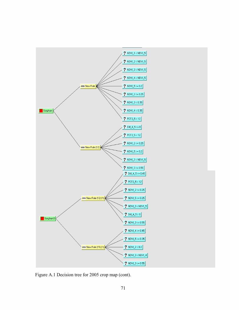
71
Figure A.1 Decision tree for 2005 crop map (cont).

72
Figure A.1 Decision tree for 2005 crop map (cont).

73
Figure A.2 Decision tree for 2006 crop map.

74
Figure A.2 Decision tree for 2006 crop map (cont).

75
Figure A.2 Decision tree for 2006 crop map (cont).
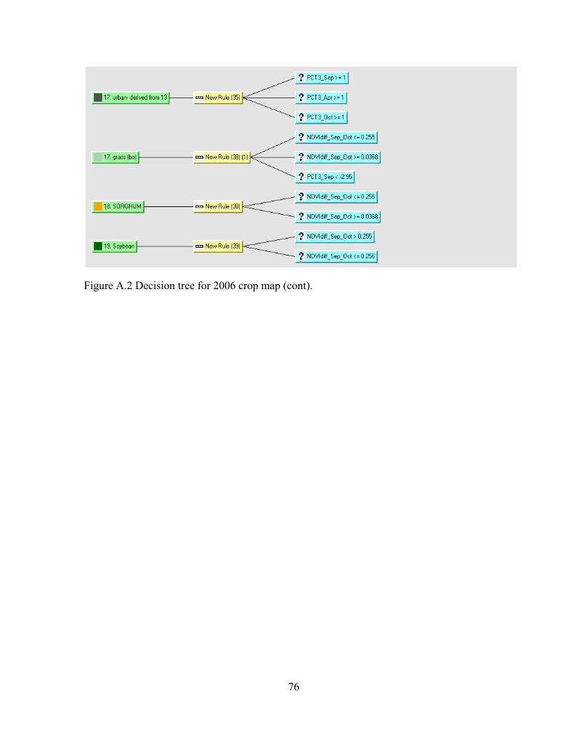
76
Figure A.2 Decision tree for 2006 crop map (cont).

77
APPENDIX B
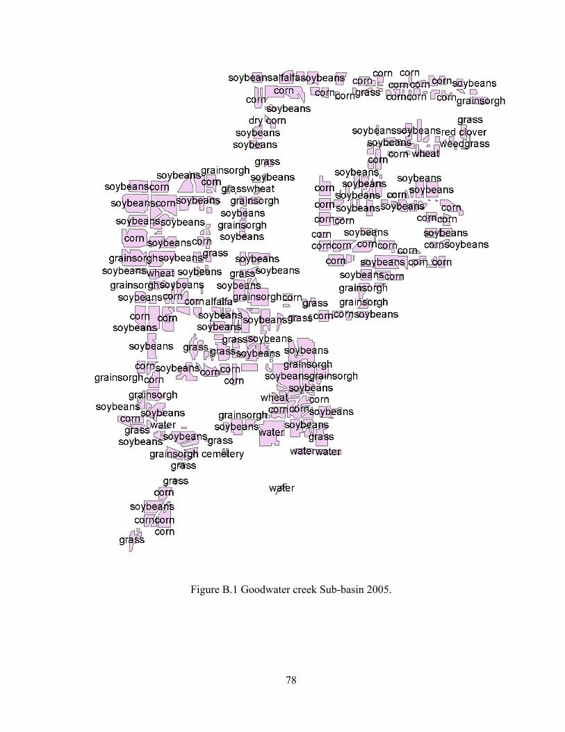
78
Figure B.1 Goodwater creek Sub-basin 2005.
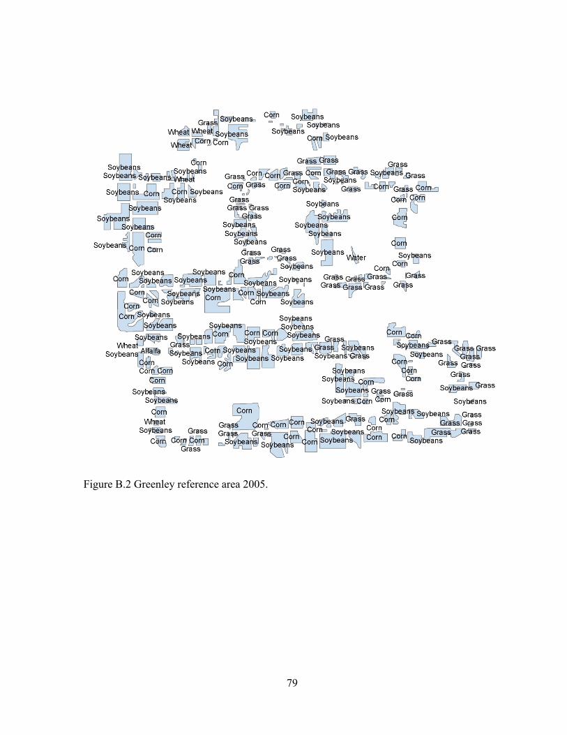
79
Figure B.2 Greenley reference area 2005.

80
Figure B.3 Goodwater creek Sub-basin 2006.

81
Figure B.4 Greenley reference area 2006.

82
APPENDIX C

83
Figure C.1 Missouri Initial planting dates – corn – 2005 crop year

84
Figure C.2 Missouri Initial planting dates – grain sorghum – 2005 crop year.
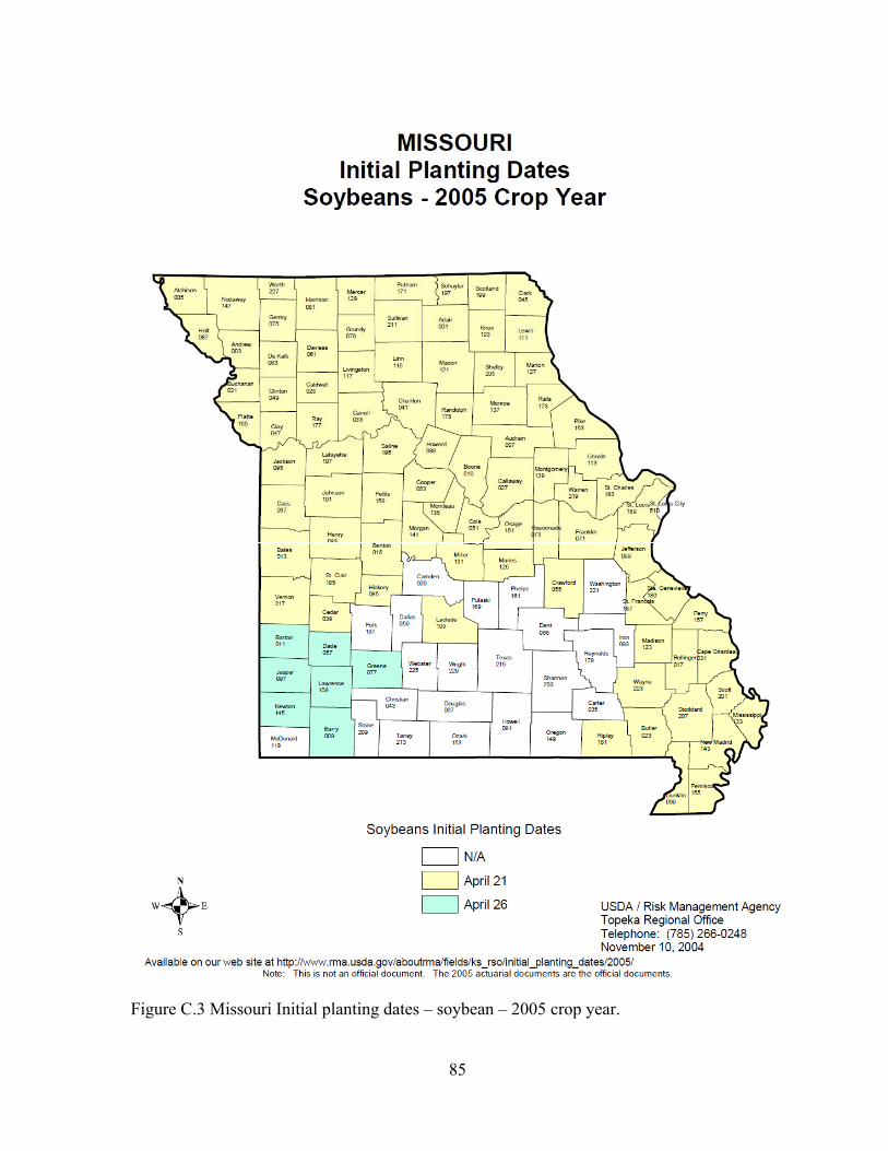
85
Figure C.3 Missouri Initial planting dates – soybean – 2005 crop year.

86
Figure C.4 Missouri Initial planting dates – corn – 2006 crop year.

87
Figure C.5 Missouri Initial planting dates – grain sorghum – 2006 crop year.

88
Figure C.6 Missouri Initial planting dates – soybean – 2006 crop year.

89
REFERENCES
Agrawal. S., P.K. Joshi, Y. Shukla and P.S. Roy. 2003. SPOT VEGETATION multitemporal data for classifying vegetation in south central Asia. Current Science. 84(11): 1440-1448.
Aplin, P. and P.M. Atkinson. 2001. Sub-pixel land cover mapping for per-field classification. International Journal of Remote Sensing. 22(14): 2853-2858.
Bauer, M.E. 1985. Spectral inputs to Crop Identification and Condition Assessment. Proceedings of the IEEE. 73(6): 1071-1085.
Brook, R. K., and N.C. Kenkel. 2002. A multivate approach to vegetation mapping of Manitoba’s Hudson Bay Lowlands. International Journal of Remote Sensing. 23(21): 4761-4776.
Choubey,V.K. and Subramanian. 1992. Estimation of suspended solids using India Remote Sensing Satellite- 1A data: a case study from Central India. International Journal of Remote Sensing. 13(8): 1473-1486.
Chubey, M.S., S.E. Franklin and M.A. Wulder. 2006. Object-based Analysis of Ikonos-2 Imagery for Extraction of Forest Inventory Parameters. Photogrammetric Engineering & Remote Sensing. 72(4): 383-394.
Cihlar, J. 2000. Land cover mapping of large area from satellite: status and research priorities. International Journal of Remote Sensing. 21(6-7): 1093-1114.
Cohen, Y. and M. Shoshany. 2002. A national knowledge-based crop recognition in Mediterranean environment. International Journal of Applied Earth Observation and Geoinformation. 4: 75-87.
Collingwood, A. 2008. Satellite Image Classification and Spatial Analysis of Agricultural Areas for Land Cover Mapping of Grizzly Bear Habitat. MS Thesis. University of Saskatchewan Saskatoon, Canada. 136 pp.
Congalton, G. R. 1991. A review of Assessing the accuracy of Classifications of Remotely Sensed data” Remote Sensing of Environment. 37: 35-46.
Craig, M. E. 2001. The NASS cropland data layer program. Presented at the third International Conference on Geospatial Information in Agriculture and Forestry. Denver, CO.
Crist, E.P. and R.C. Ciccone. 1984. A physically-based transformation of thematic mapper data-the TM tasseled cap. IEEE Transactions on Geoscience and Remote Sensing. 22: 256-263.

90
DeFries, R.S. and A.S. Belward. 2000. Global and regional land cover characterization from satellite data: An introduction to the special issue. International Journal of remote sensing. 21(6-7): 1083-1092.
De Wit, A.J.W. and J.G.P.W. Clevers. 2004. Efficiency and accuracy for per-field classification for operational crop mapping. International Journal of Remote Sensing. 25(20): 4091-4112.
Doraiswamy, C. P., B. Akhmedov, L. Beard, A. Stern and R. Mueller, 2006a. Operational prediction of crop yields using MODIS data and products. ISPRS Archives XXXVI-8/W48 Workshop proceedings: Remote sensing support to crop yield forecast and area estimate.
Doraiswamy, C. P., B. Akhmedov, L. Beard, A. J. Stern 2006b. Improved Techniques for Crop Classification using MODIS Imager, International Geoscience and Remote Sensing Symposium, pp. 2084-2087.
Finney, V.L., 1986. Seasonal sediment yield to Mark Twain Lake, Missouri. Bulletin of the Association of Engineering Geologist. 23(3): 333-338.
Foody, G.M., 2002. Status of land cover classification accuracy assessment. Remote Sensing of Environment. 80: 185-201.
Franklin, S.E. 2001. Remote sensing for sustainable forest management. Boca Raton FL: CRC/Lewis Press.
Franklin, S.E. and M.A. Wuller. 2002. Remote sensing methods in medium spatial resolution satellite data land cover classification of large areas” Progress in Physical Geography, vol. 26, no. 2, 2002, pp. 173-205.
Fried, M.A., C.E. Brodley and A.H. Strahler, 1999. Maximizing land cover classification accuracies produced by decision trees at continental to global scales. IEEE Transactions on Geoscience and Remote Sensing. 37: 969-977.
Ghidey, F., E.J. Sadler, R.N. Lerch, and C. Baffaut. 2005. Simulating hydrology and water quality of a clayoan soil watershed. ASABE Paper No. 052084. St Joseph, MI: American Society of Agricultural Engineers.
Ghidey, F., E.J. Sadler, R.N. Lerch, and C. Baffaut. 2007. Scaling up the SWAT model from Goodwater Creek Experimental Watershed to the Long Branch Watershed. ASABE Paper No. 072043. St Joseph, MI: American Society of Agricultural Engineers.
Harry, C. M. and W.J. Wiebold. 1949. Wheat-Soybean Double-crop Management in Missouri. MU extension, University of Missouri-Columbia.
Havlin, J., A. Schlegel, K.C. Dhuyvetter, J.P. Shroyer, H. Kok, and D. Peterson. 1995. Great plains dryland conservation technologiesPublication. S-81: pp. 711. Manhattan, KS: Kansas State University.

91
Homer, C., C. Huang, L. Yang, B. Wylie and M. Coan. 2004. Development of a 2001 national land-cover database for the United States. Photogrammetric Engineering and Remote Sensing, 70(7): 829-840.
Huete, A.R., 1988. A soil-adjusted vegetation index (SAVI). Remote Sensing Environment. 25: 295-309.
Huete, A.R. and C. Justive. 1999. MODIS vegetation index (MOD 13): Algorithm theoretical basis document (pp. 43-46). Tucson, Arizona: University of Arizona.
Jackson, J. Thomas, Daoyi Chen, Michael Cosh, Fuqin Li, Martha Anderson, Charles Walthall, Paul Doraiswamy, E. Ray Hunt. 2004. Vegetation water content mapping using Landsat data derived normalized difference water index for corn and soybeans. Remote Sensing of Environment, 92: 475-782.
Jang, G. S., K. A. Sudduth, E. J. Sadler and R. N.Lerch. 2009. Watershed-scale type classification using seasonal Trends in remote sensing-derived vegetation indices. American Society of Agricultural and Biological Engineers. 52(5): 1535-1544.
Jensen, J.R., Remote Sensing of the Environment: An Earth Resource Perspective. Upper Saddle River, Prentice Hall, 2000.
Jianqiang, R., Z. Chen, Q. Zhou and H. Tang “Regional yield estimation for winter wheat with MODIS –NDVI data in Shandong, China” International Journal of Applied Earth Observation and Geoinformation vol. 10, 2008, pp. 403-413.
Jiyul, C., M. C. Hansen, K. Pittman, M. Corroll, and C. DiMiceli 2007. Corn and Soybean Mapping in the United State Using MODIS Time-Series Data Sets. Agronomy Journal.99: 1654-1664.
Joshi, P.K.K., P.S. Roy, S. Singh, S. Agrawal, and D. Yadav. 2006. Vegetation cover mapping in India using multi-temporal IRS Wide Field Sensor (WiFS) data. Remote Sensing of Environment. 103: 190-202.
Kauth, R.J. and G.S. Thomas. 1976. The tasseled cap – a graphic description of the spectral-temporal development of agricultural crops as seen by Landsat. Pages 4B-41 – 4B-51 in Swain PH, Morrison DB, eds Processing of Remotely Sensed Data, Purdue University Laboratory for Applications of Remote Sensing, West Lafayette, IN, 6 June – 2 July 1976. New York: Institute of Electrical and Electonics Engneers.
Kaufman J. Y., D. Tanre 1992. Atmospherically Resistant Vegetation Index (ARVI) for EOS-MODIS. IEEE Transactions on Geoscience and Remote Sensing. 30(2): 261-270.
Kawata, Y., A. Ohtani, T. Kusaka and S. Ueno. 1990. Classification accuracy for the MOS-1 MESSR data before and after the atmospheric correction. IEEE Transactions on Geoscience and Remote Sensing. 28: 755-760.

92
Lillesand, M. T., R.W. Kiefer, J.W. Chipman, 2004. Remote Sensing and Image Interpolation, 5th Edition, John Wiley & Sons.
Lerch, E.N., E.J. Sadler, N.R. Kitchen, K.A. Sudduth, E.J. Kremer, D.B. Myers, C. Baffaut, S.H. Anderson and C.H. Lin. 2008. Overview of the Mark Twain Lake/Salt River Basin Conservation Effects Assessment Project. Journal of Soul and Water Conservation. 63(6): 345-359.
Lodhi, M.A., D.C. Rundquist, L.Han and M.S. Kuzila. 1997. The potential for remote sensing of loess soils suspended in surface waters. Journal of the American Water Resources Association. 33(1): 111-117.
Lyon, J.G., K.W. Bedford, C.J. Yen, D.H. Lee and D. J. Mark. 1988. Determinations of suspended sediment concent5rations for multiple day Landsat and AVHRR data. Remote Sensing of Environment. 25: 107-115.
McIver, D.K., and M.A. Friedl. 2002. Using prior probabilities in decision tree classification of remote sensed data. Remote Sensing of Environment. 81: 253-261.
Missouri Initial Planting Dates 2005, USDA, Risk Management Agency: www.rma.usda.gov/aboutrma/fields/ks_rso/initial_planting_datas/2005/
Missouri Initial Planting Dates 2006, USDA, Risk Management Agency: http://www.rma.usda.gov/aboutrma/fields/ks_rso/initial_planting_dates/2006/
Mosiman, B. 2003. Exploring Multi-Temporal and Transformation Methods for Improved Cropland Classification Using Landsat Thematic Mapper Imagery. Master's Thesis, Department of Geography, University of Kansas, Lawrence, KS.
Mueller, R., C. Boryan, R. Seffrin. 2009. Data Partnership Synergy: The cropland Data Layer. US Department of Agriculture, National Agricultural Statistics Service. Fairfax, VA.
Murthy, C.S, P.V. Raju and K.V.S. Badrinath. 2003. Classification of wheat crop with multi-temporal images: performance of maximum likelihood and artificial neural networks. International Journal of Remote Sensing. 24(23): 4871-4890.
Reese, H.M, T.M. Lillesand, D.E. Nagel, J.S. Stewart, R.A. Goldmann, T.E. Simmons, J.W. Chipman and P.A. Tessar. 2002. Statewide land cover derived from multi-seasonal Landsat TM data: A retrospective of the WISLAND project. Remote Sensing of Environment. 82: 224-237.
Richards, J.A. and X. Jia. 2006. Remote Sensing Digital Image Analysis – An introduction. 4th Edition. Springer. Canberra, Australia.
Rogers, D. H. 1997. Soybean production handbook. Publication, Vol. C-449 (pp. 1519). Kansas State University. Manhattan, KS.

93
Running, S.W., T.R. Loveland and L.L. Pierce. 1994. A vegetation classification logic based on remote sensing for use in global biogeochemical models. Ambio. 23: 77-81.
SBRC, 1994, Space sensors. Goleta, CA: Santa Barbara Research Center, 33 pp.
Skadeland, T. 1992. Water Quality and Land Cover Types in the Upper Salt River Basin. MS Thesis, University of Missouri-Columbia, 118 pp.
Soil Conservation Service. 1974. Soil survey of Marion and Ralls counties, Missouri. U.S. Government Print. Off. 1979:-207-350/122.
Soil Conservation Service. 1979. Soil survey of Knox, Monroe, and Shelby counties, Missouri. U.S. Government Print. Off. 1979:-207-350/122.
Soil Conservation Service. 1989. Soil survey of Marion and Randolph county, Missouri. U.S. Government Print. Off. 1989: 0-205-522.
Song C., C.E. Woodcock, K.C. Seto, M.P. Lenney, and S.A. Macomber, 2001. Classification and Change Detection Using Landsat TM Data: When and How to correct Atmospheric Effects? Remote Sensing of Environment, 75: 230-244.
Stephen B.A. 2000. Remote Sensing of Suspended Solid and Turbidity in Mark Twain Lake, Missouri. MA Thesis. University of Missouri-Columbia. 112 pp.
Tou, D. L. and R.C. Gozalez. 1974. Pattern Recognition Principles. London, U.K.: Addison-Wesley.
USDA, National Agricultureal Statistic Service, 2005: Quick stats agricultural statistic data base.www.nass.usda.gov/data_and_statistics/
USDA, National Agricultureal Statistic Service, Missouri, Farm Facts publication: http://www.nass.usda.gov/Statistics_by_State/Missouri/Publications/Farm_Facts/
Vanderlip, R., D.H. Rogers and M. Alam. 1998. Grain sorghum production guide. Publication, Vol. C-687. pp. 1518. Kansas State University. Manhattan, KS.
Van Niel, T.G. and T.R. McVicar. 2004. Determining temporal windows for crop discrimination with remote sensing: a case study in south-eastern Australia. Computers and Electronics in Agriculture. 45: 91-108.
Van Niel, T.G., T.R. McVicar and B. Datt. 2005. On the relationship between training sample size and data dimensionality: Monte Carlo analysis of broadband multi-temporal classification. Remote Sensing of Environment. 98: 468-480.
Wang, J., P.M. Rich, K.P. Price, W.D. Kettle, 2005. Relations between NDVI, Grassland Production, and Crop Yield in the Central Great Plains. Geocarto International, 20(3): 5-11.

94
Wardlow, D.B. and S.L. Egbert 2005. State-level crop mapping in the U.S. Central Great Plains Agroecosystem using MODIS 250-meter NDVI data.
Wardlow, D. B., S.L. Egbert and J.H. Kastens. 2007. Analysis of time-series MODIS 250 m vegetation index data for crop classification in the U.S. Central Great Plains” Remote Sensing of Environment.108: 290-310.
Walter, V. 2004. Object-based classification of remote sensing data for change detection. ISP RS Journal of Photogrammetry & Remote Sensing. 58: 225-238.
Yamamoto, Y., T. Oberthur, R. Lefroy. 2009. Spatial identification by satellite imagery of the crop-fallow rotation cycle in northern Laos. Environ Dev Sustain. 11: 639-654.
Zhang, X., M.A. Friedl, C.B. Schaaf, A.H. Strahler,J.C.F. Hodges, and F. Gao. 2003. Monitoring vegetation phenology using MODIS. Remote Sensing of Environment. 84: 471-475.