Development of Laboratory to Field Shift Factors for Hot-Mix Asphalt Resilient Modulus

by

Samer W. Katicha

Thesis submitted to the Faculty of the

Virginia Polytechnic Institute and State University

In partial fulfillment of the requirements for the degree of

Masters Of Science

in

Civil Engineering

Imad L. Al-Qadi, Chair

Gerardo Flintsch

Amara Loulizi

November 2003

Blacksburg, Virginia

Keywords: resilient modulus, hot-mix asphalt, temperature, compaction

Copyright by Samer W. Katicha 2003

Development of Laboratory to Field Shift Factors for Hot-Mix Asphalt Resilient Modulus

Samer W. Katicha

Virginia Polytechnic Institute and State University

Advisor: Imad L. Al-Qadi

Abstract

Resilient moduli of different surface mixes placed at the Virginia Smart Road were

determined. Testing was performed on Field cores (F/F) and laboratory-compacted

plant mixed (F/L), laboratory mixed and compacted per field design (L/L), and laboratory

designed, mixed, and compacted (D/L) specimens. The applied load was chosen to

induce a strain ranging between 150 and 500 microstrains. Two sizes of laboratory

compacted specimens (100-mm in diameter and 62.5-mm-thick and 150-mm in diameter

and 76.5-mm-thick) were tested to investigate the effect of specimen size on the resilient

modulus. At 5oC, the measured resilient moduli for both specimen sizes were similar.

However, the specimen size has an effect on the measured resilient modulus at 25 and

40oC, with larger specimens having lower resilient modulus. At 5oC, HMA behaves as

an elastic material; correcting for the specimen size using Roque and Buttlar’s correction

factors is applicable. However, at higher temperatures, HMA behavior becomes

relatively more viscous. Hence, erroneous resilient modulus values could result when

elastic analysis is used. In addition, due to difference in relative thickness between the

100- and 150-mm diameter specimens, the viscous flow at high temperature may be

different. In general, both specimen sizes showed the same variation in measurements.

Resilient modulus results obtained from F/L specimens were consistently higher than

those obtained from F/F specimens. This could be due to the difference in the

volumetric properties of both mixes; where F/F specimens had greater air voids content

than F/L specimens. A compaction shift factor of 1.45 to 1.50 between the F/F and F/L

specimens was introduced. The load was found to have no effect on resilient modulus

under the conditions investigated. However, the resilient modulus was affected by the

load pulse duration. The testing was performed at a 0.1s and 0.03s load pulses. The

resilient modulus increased with the decrease of the load pulse duration at temperatures

of 25oC and 40oC, while it increased at 5oC. This could be due to the difference in

specimen conditioning performed at the two different load pulses. Finally, a model to

predict HMA resilient modulus from HMA volumetric properties was developed. The

model was tested for its fitting as well as predicting capabilities. The average variability

between the measured and predicted resilient moduli was comparable to the average

variability within the measured resilient moduli.

iv

To my father,

Wehbe Katicha,

my mother,

Nelly Katicha,

and my sister and brother

Nathalie and Nabil

v

Acknowledgments

First I would like to thank my advisor, Dr. Imad L. Al-Qadi, for his help and

patience throughout my graduate studies. His guidance and support made my

working and learning experience, a very special one. In addition, I would like to

thank Dr. Gerardo Flintsch and Dr. Amara Loulizi for their support and help as

members of my advisory committee.

Also, I would like to thank my colleagues Alex Appea, Moustafa Elseifi, Samer

Lahour, Stacey Reubush, Edgar De Leon Izeppi, Kevin Siegel, and Alan Christoe

at the Roadway Infrastructure Group at the Virginia Smart Road. The good

discussions we had, whether related to pavements or football games, made my

learning experience much more enjoyable. Last but not least, I would like to

extend my thanks to William (Billy) Hobbs, better known as “The Man”, for

preparing the samples and fixing the MTS whenever I break it.

Samer W. Katicha

vi

Table of Content

Abstract ........................................................................................................v

Acknowledgments ..............................................................................................v

List of Figures ..................................................................................................viii

List of Tables...................................................................................................... ix

Chapter 1 Introduction ...................................................................................1 1.1 Introduction .....................................................................................................1 1.2 Background .....................................................................................................2

1.2.1 Flexible Pavements ...................................................................................2 1.2.2 Flexible Pavement Design.........................................................................3 1.2.3 Failure Criteria in Flexible Pavements.......................................................4

1.3 Material Characterization................................................................................5 1.3.1 Dynamic Complex Modulus.......................................................................5 1.3.2 Resilient Modulus ......................................................................................6 1.3.3 Creep Compliance.....................................................................................7

1.4 Problem Statement and Research Objective................................................7 1.5 Scope................................................................................................................8

Chapter 2 Present State of Knowledge .........................................................9 2.1 Flexible Pavement and Their Main Design Factors......................................9

2.1.1 Input Design Parameters.........................................................................10 2.2 Material Characterization..............................................................................12

2.2.1 Resilient Modulus ....................................................................................13 2.2.2 Indirect Tension Test ...............................................................................14

2.3 Factors Affecting Resilient Modulus Results .............................................16 2.3.1 Mix Components Effect ...........................................................................16 2.3.2 Loading Effect..........................................................................................17 2.3.3 Effect of Poisson’s Ratio..........................................................................18 2.3.4 Effect of Testing Axis...............................................................................19 2.3.5 Specimen Size Effect ..............................................................................20 2.3.6 Effect of Measuring Devices....................................................................20 2.3.7 Effect of Moisture.....................................................................................22

2.4 Resilient Modulus Data Analysis Methods .................................................23 2.4.1 Hondros’ 2-D Plane Stress Solution ........................................................23 2.4.2 Roque and Buttlar’s Indirect Tension Specimen Analysis .......................29 2.4.3 Three Dimensional Solution for the Indirect Tensile Test........................31

2.5 Summary ........................................................................................................34

Chapter 3 Research Approach ....................................................................35 3.1 Introduction ...................................................................................................35

vii

3.2 Virginia Smart Road ......................................................................................35 3.3 Hot Mix Asphalt Preparation ........................................................................37

3.3.1 Specimen Designation and Characteristics.............................................38 3.3.2 Specimen Preparation .............................................................................40 3.3.3 Laboratory Compaction ...........................................................................41

3.4 Specimen Testing..........................................................................................42 3.4.1 Loading....................................................................................................45 3.4.2 Testing and Data Collection ....................................................................45 3.4.3 Indirect Tensile Strength Test..................................................................47

3.5 Resilient Modulus Calculations ...................................................................47 3.5.1 Roque and Buttlar’s Procedure for Resilient Modulus Calculation ..........48 3.5.2 Three-Dimensional Solution ....................................................................50

3.6 Research Methodology.................................................................................53 3.6.1 Test Variability .........................................................................................53 3.6.2 Shift Factors ............................................................................................54 3.6.3 Resilient Modulus Prediction from Volumetric Properties........................54

Chapter 4 Results and Analysis ..................................................................56 4.1 Introduction ...................................................................................................56 4.2 Load Determination.......................................................................................56 4.3 Resilient Modulus Results............................................................................61 4.4 Variability .......................................................................................................65

4.4.1 Within Specimen Variation ......................................................................66 4.4.2 Within Mix Variation.................................................................................67

4.5 Shift Factors ..................................................................................................68 4.5.1 Compaction Shift Factor ..........................................................................69 4.5.2 Specimen Size Shift Factor: ....................................................................72 4.5.3 Loading Duration Shift Factor..................................................................75

4.6 Resilient Modulus Prediction from Volumetric and Binder Properties ....78 4.6.1 Factors Affecting Resilient Modulus ........................................................79 4.6.2 Model Development.................................................................................81 4.6.3 Model Evaluation .....................................................................................84 4.6.4 Resilient Modulus Calculation for F/F Specimens ...................................86

4.7 Conclusion.....................................................................................................88

Chapter 5 Findings, Conclusions, and Recommendations.......................90 5.1 Summary ........................................................................................................90 5.2 Findings .........................................................................................................91 5.3 Conclusions...................................................................................................93 5.4 Recommendations ........................................................................................93

References ......................................................................................................95

Appendix A ......................................................................................................97

Appendix B ....................................................................................................142

Appendix C ....................................................................................................154

Vitae ....................................................................................................162

viii

List of Figures

Figure 1-1 Flexible pavement cross-section. ..............................................................3 Figure 2-1 Elastic stress distribution in indirect tension specimen............................21 Figure 2-2 Illustration of Bulging Effects ...................................................................30 Figure 3-1 Structural configuration of Virginia Smart Road. .....................................37 Figure 3-2 Troxler Gyratory Compactor. ...................................................................41 Figure 3-3 Extensiometer Mounting..........................................................................43 Figure 3-4 Test configuration of the Indirect Tension Test .......................................44 Figure 3-5 Collected Data for Resilient Modulus Testing..........................................46 Figure 4-1 Stress Distribution ...................................................................................66 Figure 4-2 Compaction shift factor............................................................................70 Figure 4-3 Specimen size shift factor (a) F/L specimens, (b) L/L specimens, and (c)

D/L specimens ........................................................................................................73 Figure 4-4 Load Duration Shift Factor.......................................................................77 Figure 4-5 Resilient Modulus Variation with Temperature (Specimen A1-4in D/L)...79 Figure 4-6 Calculated vs. Measured Mr ....................................................................86

ix

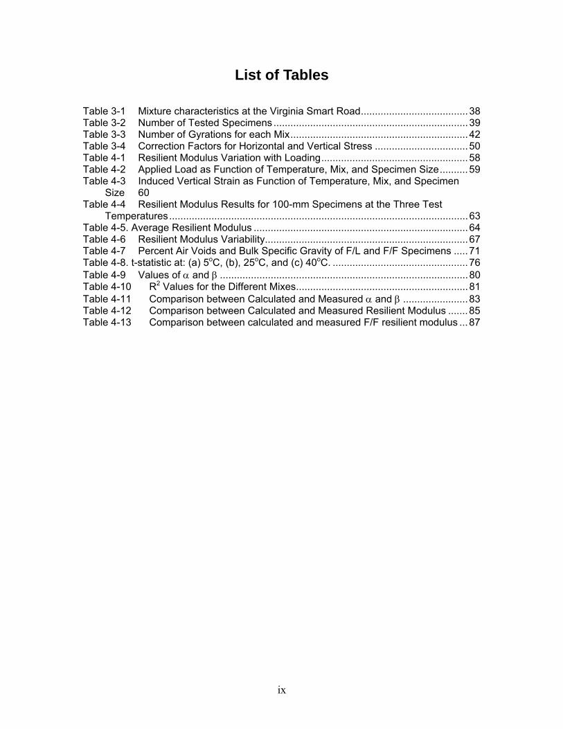
List of Tables

Table 3-1 Mixture characteristics at the Virginia Smart Road......................................38 Table 3-2 Number of Tested Specimens .....................................................................39 Table 3-3 Number of Gyrations for each Mix...............................................................42 Table 3-4 Correction Factors for Horizontal and Vertical Stress .................................50 Table 4-1 Resilient Modulus Variation with Loading....................................................58 Table 4-2 Applied Load as Function of Temperature, Mix, and Specimen Size..........59 Table 4-3 Induced Vertical Strain as Function of Temperature, Mix, and Specimen

Size 60 Table 4-4 Resilient Modulus Results for 100-mm Specimens at the Three Test

Temperatures..........................................................................................................63 Table 4-5. Average Resilient Modulus ............................................................................64 Table 4-6 Resilient Modulus Variability........................................................................67 Table 4-7 Percent Air Voids and Bulk Specific Gravity of F/L and F/F Specimens .....71 Table 4-8. t-statistic at: (a) 5oC, (b), 25oC, and (c) 40oC. ................................................76 Table 4-9 Values of α and β ........................................................................................80 Table 4-10 R2 Values for the Different Mixes.............................................................81 Table 4-11 Comparison between Calculated and Measured α and β .......................83 Table 4-12 Comparison between Calculated and Measured Resilient Modulus .......85 Table 4-13 Comparison between calculated and measured F/F resilient modulus ...87

1

Chapter 1 Introduction

In this chapter an overview of the pavement material characterization is

discussed. Hot mix asphalt (HMA) mixtures were tested to determine the creep

compliance, fatigue resistance, and resilient modulus of the different mixes which are

key input parameters in pavement design and rehabilitation. The characterization of

HMA depends on the way the material is obtained. This will lead to the formulation of

the problem statement, which will be followed by the research objectives. A summary of

the research scope is briefly presented at the end of the chapter.

1.1 Introduction

The Mechanistic-Empirical design of flexible pavements is based on limiting the

distresses in the pavement structure. Pavement distresses are caused by the different

types of loadings mainly structural and environmental loadings. Environmental loadings

are mainly addressed in the selection of the asphalt binder. The structural loading

distresses are mainly fatigue cracking and permanent deformation (rutting). Although

these two distresses are caused by the structural loading (vehicular loading on the

pavement structure), they are also affected by the environmental conditions. The

mechanistic-empirical pavement design method requires limiting the cracking and rutting

in the pavement structure. Many factors affect the ability of the HMA to meet these

structural requirements. These are the different components (aggregates and binders)

of the HMA, their interaction, the mix design, and the method of preparation. Great

efforts have been made to better understand HMA behavior. However, with the

increasing use of new technologies (e.g. modifiers in the binder, and reinforcement of

the pavement) and establishment of new design specifications, much work still needs to

be done to characterize HMA mixtures. Hot-mix asphalt mixes are primarily designed to

resist permanent deformation and cracking. The ability of the HMA to meet those

requirements depends on the following:

• The binder characteristics;

• Aggregate characteristics and gradation;

• Modifiers;

• Temperature;

• Moisture;

2

• Loading (load level, rate, and the loading rest time);

• Aging characteristics;

• State of stress (tension vs. compression, uniaxial, biaxial or Triaxial);

• Compaction method.

1.2 Background

1.2.1 Flexible Pavements

Flexible pavements are designed to provide a smooth surface and reduce the

stresses on the natural subgrade. Good quality materials are used at the top of the

layered pavement system to reduce the vehicular induced stresses with depth. Inferior

materials are used at the bottom where the stresses are low. This design approach

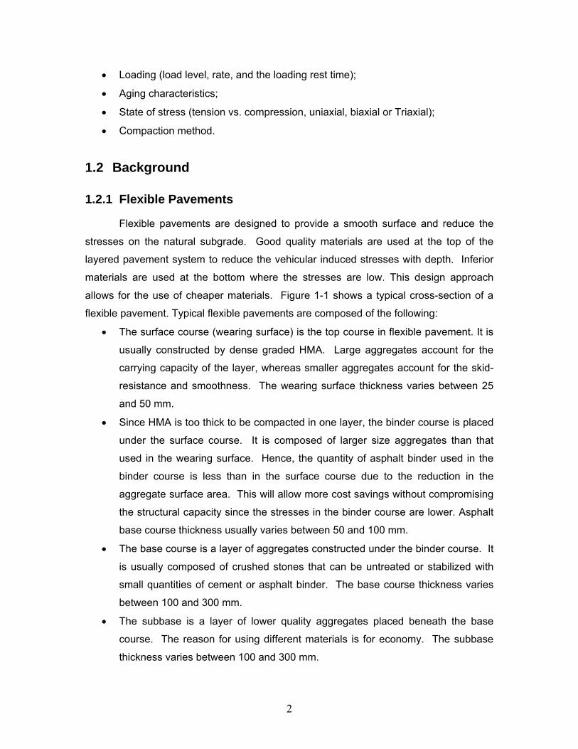
allows for the use of cheaper materials. Figure 1-1 shows a typical cross-section of a

flexible pavement. Typical flexible pavements are composed of the following:

• The surface course (wearing surface) is the top course in flexible pavement. It is

usually constructed by dense graded HMA. Large aggregates account for the

carrying capacity of the layer, whereas smaller aggregates account for the skid-

resistance and smoothness. The wearing surface thickness varies between 25

and 50 mm.

• Since HMA is too thick to be compacted in one layer, the binder course is placed

under the surface course. It is composed of larger size aggregates than that

used in the wearing surface. Hence, the quantity of asphalt binder used in the

binder course is less than in the surface course due to the reduction in the

aggregate surface area. This will allow more cost savings without compromising

the structural capacity since the stresses in the binder course are lower. Asphalt

base course thickness usually varies between 50 and 100 mm.

• The base course is a layer of aggregates constructed under the binder course. It

is usually composed of crushed stones that can be untreated or stabilized with

small quantities of cement or asphalt binder. The base course thickness varies

between 100 and 300 mm.

• The subbase is a layer of lower quality aggregates placed beneath the base

course. The reason for using different materials is for economy. The subbase

thickness varies between 100 and 300 mm.

3

• The subgrade is the bottom layer of compacted in-situ soil or selected material.

The subgrade should be compacted at the optimum moisture content to get a

high density.

(a) Regular pavement (b) Full depth pavement

Figure 1-1 Flexible pavement cross-section.

It should be noted that the use of the various layers is based on either the

necessity (vehicular and environmental loading) or economy (materials cost and

availability, and construction constraints). Therefore, the number of layers in a

pavement system could vary. In some cases, full depth pavement shown in Figure 1-1

(b) may be considered.

1.2.2 Flexible Pavement Design

Pavement response to loading and performance require the proper

characterization of paving materials. Hot mix asphalt is a viscoelastic material, which

means that its stress-stain relationship is time and temperature-dependent. Pavements

have been analyzed using different theories such as the elastic, the viscoelastic, and the

viscoplastic theory. It has become of practice that different pavement responses are

predicted using different theories. For example, viscoelastic theory is used to predict

thermal stresses and strains as well as permanent deformation. In this case the time

and temperature dependant stiffness is used as a material characteristic input. On the

other hand, load-induced stresses and strains can be accurately predicted by linear

elastic layer theory at temperatures below about 30oC (Roque and Buttlar, 1992).

Material characterization in elastic theory requires the determination of two parameters

which are the elastic modulus and Poisson’s ratio.

Wearing surface (25 - 50 mm.)

Asphalt base course (50 - 100 mm.)

Base course (100 – 300 mm.)

Subbase course (100 – 300 mm.)

Subgrade

Wearing surface (25 - 50 mm.)

Asphalt base course (50 – 500 mm.)

Subgrade

4

The elastic modulus has been traditionally determined in the field using deflection

obtained from non destructive tests such as the Falling Weight Deflectometer (FWD).

However, moduli determined through back calculation are for a specific temperature at

which the test was performed. Although generalized relationships between HMA elastic

modulus and temperature have been developed, their use can lead to considerable error

since these relationships can vary between one asphalt mix and another. Moreover, it

has been shown that near surface layer moduli determined using deflection basins from

FWD testing are not accurate. These problems can be overcome in the laboratory

where materials from each layer can be tested at a controlled temperature. Material

properties determined in the laboratory can vary considerably from one test setup to

another. Proper material properties are obtained when the laboratory setup induces

stress states that are similar to the ones experienced in the filed.

Testing in the lab can be performed on field specimens or laboratory-produced

specimens. Differences have been shown to exist between field and laboratory-

produced specimens using different methods of compaction. Gyratory compaction has

been proven to better correlate with field compaction than other methods (Button et al.,

1994). The gyratory compaction is the one used in the Superpave design protocol, and

will be used in the following research.

1.2.3 Failure Criteria in Flexible Pavements

Fatigue Cracking:

Fatigue cracking of flexible pavements is thought to be based on the horizontal

tensile strain at the bottom of the HMA layer. The failure criterion relates the allowable

number of load repetitions to the tensile strain. The cracking initiates at the bottom of

the HMA where the tensile strain is highest under the wheel load. The cracks propagate

initially as one or more longitudinal parallel cracks. After repeated heavy traffic loading,

the cracks connect in a way resembling the skin of an alligator. Laboratory fatigue tests

are performed on small HMA beam specimens. Due to the difference in geometric and

loading conditions; especially rest period between the laboratory and the field, the

allowable number of repetitions for actual pavements is greater than that obtained from

laboratory tests. Therefore, the failure criterion may require incorporating a shift factor to

account for the difference.

5

Rutting:

Rutting is indicated by the permanent deformation along the wheelpath. Rutting

can occurs in any of the pavement layers or the subgrade, usually caused by the

consolidation or the lateral movement of the materials due to traffic loads. Rutting in the

HMA layer is controlled by the creep compliance of the mix. Rutting occurring in the

subgrade is caused by the vertical compressive strain at the top of the subgrade layer.

To control rutting occurring in the subgrade, the vertical compressive strain at the top of

the subgrade is limited to a certain value.

It is noticed that fatigue cracking and rutting depend on the level of strain; tensile

strain at the bottom of the HMA layer for fatigue cracking, and compressive strain at the

top of the subgrade layer for rutting. Therefore, to be able to predict the fatigue as well

as the rutting lives of the pavement structure, the aforementioned strains must be

determined. Load induced stresses and strains in pavements are determined using the

elastic layered theory. This requires the determination of the moduli of the different

layers in the pavement structure. Moduli are usually determined in the field by

performing the FWD test. However, near surface moduli (modulus of the wearing

surface) are difficult to obtain using FWD results. Moreover, for the design of the

pavement, layers moduli must be determined prior to the pavement is construction.

1.3 Material Characterization

Hot mix asphalt can be characterized as either a viscoelastic or an elastic

material. Viscoelastic characterization involves measuring the dynamic complex

modulus and the creep compliance. Elastic characterization involves measuring the

resilient modulus. Since HMA’s properties are functions of time and temperature, its

characterization should reflect this fact.

1.3.1 Dynamic Complex Modulus

The dynamic complex modulus has been used for the design of pavements

(Shook, 1969). The complex modulus test performed in the laboratory by applying a

sinusoidal or haversine loading with no rest period. This testing approach is one of

many methods for describing the stress-strain relationship of viscoelastic materials. The

dynamic complex modulus is composed of two parts: the real part, which represents the

elastic stiffness and the imaginary part, which represents the internal damping due to the

6

viscoelastic properties of the material. The absolute value of the complex modulus is

referred to as the dynamic modulus of HMA. The axial strains are measured using two

strain gauges. The ratio between the axial stress and the recoverable strain is the

dynamic elastic modulus. The dynamic complex modulus is determined from the

dynamic modulus and the phase angle. The phase angle being the lag between the

stress and strain maximum values.

The dynamic complex modulus test, ASTM D3497-79 (ASTM, 2003), is usually

conducted on cylindrical specimens subjected to a compressive haversine loading

varying with the loading frequency. The testing mode selected will have an effect on the

design if the design is based on the viscoelastic theory; in such a case the loading and

frequency should be selected such that it best simulates the traffic loading. Most of the

dynamic modulus tests use a compressive load applied to the specimen. However,

other tests have also been used such as the tension and tension-compression tests. A

haversine load is applied to the specimen for a minimum of 30s not exceeding 45s at

temperatures of 5, 25, and 40oC and a load frequency of 1, 4, and 16 Hz for each

temperature.

The test is affected by the setup and the effect becomes more prominent at

higher temperatures. Therefore if a design is based on elastic theory with a given

dynamic modulus for HMA, the three different testing temperature results may be used.

1.3.2 Resilient Modulus

The resilient modulus is the elastic modulus used in the layered elastic theory for

pavement design. Hot mix asphalt is known to be a viscoelstic material and, therefore,

experiences permanent deformation after each application of the load. However, if the

load is small compared to the strength of the material and after a relatively large number

of repetitions (100 to 200 load repetitions), the deformation after the load application is

almost completely recovered. The deformation is proportional to the applied load and

since it is nearly completely recovered it can be considered as elastic.

The resilient modulus is based on the recoverable strain under repeated loading and is

determined as follows:

r

drM

εσ

=

7

where σd is the deviator stress and εr is the recoverable (resilient strain). Because the

applied load is usually small compared to the strength of the specimen, the same

specimen may be used for the same test under different loading and temperatures.

The resilient modulus is evaluated from repeated load tests. Different types of

repeated load tests have been used to evaluate the resilient modulus of HMA. The most

commonly used setups are the uniaxial tension, the uniaxial compression, the beam

flexure, the triaxial compression, and the indirect diametral tension (IDT). The IDT setup

has a main advantage in its ability to simulate the stress states that exist at the bottom of

the HMA layer underneath the applied wheel load, which are of concern in pavement

design. The state of stress in an IDT specimen is rather complex, however extensive

research has been performed to address this subject, and data analysis methods are

available to accurately predict stresses and strains (Roque and Buttlar, 1992; Kim, et al.,

2002).

The resilient modulus can be performed on laboratory prepared specimens or

field cores. For consistency in design, results obtained from laboratory prepared

specimens should match with results obtained from field cores.

1.3.3 Creep Compliance

The creep test is used to characterize linear viscoelastic materials. Viscoelastic

materials such as hot mix asphalt experience an increase in total deformation as the

applied load is sustained. This phenomenon is time and temperature dependent. The

creep compliance is defined as the ratio of the instantaneous strain over the applied

stress. Creep testing is used to characterize permanent deformation. Test setups that

have been used are uniaxial (Van de Loo, 1978) and more recently indirect tension

(Roque and Buttlar, 1992; Buttlar and Roque, 1994; Wen and Kim, 2002; Kim, et al.,

2002). The advantages and disadvantages of the IDT setup for creep testing are the

same as for resilient modulus testing.

Specimen compaction is an important parameter that affects the dynamic

modulus, resilient modulus, and creep compliance laboratory results.

1.4 Problem Statement and Research Objective

Gyratory compaction was introduced by the Strategic Highway Research

Program (SHRP) as the compaction method that best replicates compaction performed

8

in the field. However, correlation between laboratory compacted HMA specimens

properties and field compacted HMA properties are not well established. Discrepancies

between laboratory prepared specimens and field cores are not solely due to

compaction; differences between the designed and as built mixes system can be quiet

significant. Specimens in the laboratory can be prepared to conform to the designed or

the as built pavement. Therefore, the development of correction factors between

laboratory-prepared specimens and specimens obtained from the field will provide

valuable information for adjusting design procedures. Hence, better prediction of

pavement performance can be achieved.

The main objective of this research was to develop shift factors to correlate

laboratory-determined resilient moduli of field cores to those of laboratory-prepared

specimens. These factors could be dependent on compaction method, specimen size,

temperature, mix production, and loading.

1.5 Scope

This research attempted to quantify the variations in resilient modulus results due

to different parameters. These parameters are specimen size, load pulse duration,

temperature, and method of production and compaction. The most important task was

to develop shift factors to relate resilient modulus of laboratory-prepared specimens to

resilient modulus of field cores. Chapter 1 is an introduction to the subject. Chapter 2

presents an overview of the present stage of knowledge regarding resilient modulus

testing and the parameters affecting its values. The resilient modulus results depend

on the analysis method used. The analysis method used should be the one that gives

the best representation of the state of stress in the specimen. The different analysis

methods available are discussed in chapter 2. In Chapter 3 the research approach is

outlined and details on specimen preparation, testing, and analysis of the results are

presented. The material used were obtained either directly from the Virginia Smart

Road, in form of road cores or loose-bagged mixture samples collected during

construction, or were produced in the laboratory from raw materials to meet design

specifications. The research results and interpretation are presented in Chapter 4.

Finally, the conclusions and recommendations are presented in Chapter 5. The research

determin specimen size shift factors (100- and 150-mm samples), Load duration shift

factors, and the relationship between the resilient modulus and the HMA properties.

9

Chapter 2 Present State of Knowledge

This chapter considers the present state of knowledge regarding flexible pavements,

materials characterization, factors affecting resilient modulus results, and methods of

analysis.

2.1 Flexible Pavement and Their Main Design Factors

By their very nature, pavement structures must be relied upon to perform

successfully and simultaneously serve several functions, among them carrying capacity,

riding comfort, safety, skid resistance, and surface drainage. While loads applied on top

of the pavement cause stresses throughout its layers, they are particularly higher at the

top than at the bottom. Therefore, in the most sensible and cost effective pavement

designs, stronger and more expensive material is placed on the top to receive the brunt

of stresses while weaker, less expensive material is placed at the bottom, where

stresses are lower. The resulting flexible pavement structure generally consists of the

following:

• Surface course or wearing surface

• Binder course

• Base and subbase course

• Subgrade

The wearing surface is the top layer of pavement, which must be strong enough

to resist stresses applied on it but at the same time provide a smooth ride. The general

mix design for wearing surfaces is a dense graded HMA. Additionally, such a layer must

minimize infiltration of water which can also achieved by providing a drainage layer.

The binder course or second layer is similar in nature to the wearing surface in

that it is a HMA. The difference between the binder and surface mixes is that in order to

reduce cost, larger aggregates and less asphalt binder are used in the former. The

larger aggregate size also provides greater strength. A base HMA may also be used.

The base course is a layer beneath the HMA layer. It is composed of crushed

material, sometimes stabilized by either Portland cement or asphalt. The subbase, a

layer of lower quality, cost-efficient material placed under the base course, often serves

as a filter between the base and subgrade.

10

The subgrade is a prepared in situ soil. It is usually compacted near the optimum

moisture content.

2.1.1 Input Design Parameters

Successful pavement designs recognize three major parameters: traffic and

loading, material properties, and environment.

Traffic and Loading:

The traffic and loading design involves axle loads, number of repetitions, tire

contact areas, and vehicle speed.

The most common axle configurations are single axle with single tires, single

axle with dual tires, tandem axles with dual tires, and tridem axles with dual tires.

Because analyzing multiple axles proves difficult, the Equivalent Single Axle Loads

(ESALs) method, which involves a standard 80-kN (18-kip) single-axle load, is used.

Design of the pavement is based on the number of ESAL repetitions that can take place

before pavement failure occurs in the form of either cracking or rutting. The applied

truck load is distributed over the tire contact area. The tire contact area is calculated by

dividing the applied load by the tire contact pressure. For simplicity the tire contact

pressure is usually taken to be equal to the tire pressure.

Finally, due to the viscoelastic nature of HMA, vehicle speed also is important to

loading. When a load is applied, viscoelastic materials, like HMA, exhibit deformations

that are time dependent. The duration of the applied truck load in the HMA layer

depends on the truck speed. In the elastic theory of pavement design and analysis, the

resilient modulus selected for each pavement layer should reflect the vehicle speed; in

other words, in calculating the resilient modulus of the HMA layer—whether in the field

or in the laboratory—the duration of the load pulse is function of the vehicle speed.

Higher speeds result in lower loading times and, therefore, smaller strains and larger

resilient modulus. Therefore, to accurately determine the resilient modulus of HMA, the

loading time that is achieved in the filed, under highway speed, should be used in the

test.

Material Properties:

In the linear elastic theory, the elastic modulus and Poisson’s ratio are used to

characterize each layer. Because the elastic modulus of HMA varies with the time of

11

loading (due to the viscoelastic nature of HMA), the resilient modulus is selected in the

analysis.

In the viscoelastic theory, creep compliance is measured by the time-temperature

shift factor, which accounts for differences between test temperature and that of the

actual pavement.

Environment:

Three major environmental factors affect pavement design: temperature,

moisture level, and frost penetration. The HMA resilient modulus is affected most by

temperature; the subgrade resilient modulus, by moisture content. Frost penetration on

the other hand affects the entire pavement system.

At high temperatures, the HMA layer becomes viscous in nature, while at low

temperatures, it becomes elastic. In flexible pavements, low temperatures cause

cracking, while high temperatures cause permanent deformation. Frost penetration

results in a stronger subgrade during winter and a weaker subgrade during spring. The

spring reduction in subgrade strength occurs when ice that has formed during colder

weather melts and leaves the subgrade saturated with water. The moisture level will

affect the strength of the subgrade. Moisture content above optimum will result in a

lower subgrade modulus.

Pavement Distresses:

Before 2002, the AASHTO pavement design method was based on the Present

Serviceability Index (PSI). However, the mechanistic-empirical (ME) pavement design

has gained enough recognition as an acceptable alternative that it has become part of

the 2002 AASHTO guide. In the M-E pavement design method, failure criteria are

established using specific types of distresses: fatigue cracking, rutting, and low

temperature cracking.

Fatigue cracking results from the repeated application of a heavy load on the

pavement structure. Such repeated application creates tensile strain at the bottom of

the HMA layer, which ultimately causes cracks to develop. The failure criterion is based

on a laboratory fatigue test to relate the allowable number of load repetitions to the

tensile strain.

Rutting is characterized by a surface depression along the wheel path. It is

associated primarily with vertical compressive strain on top of the subgrade; however, it

12

can also occur as a result of weakness in other pavement layers one of which is the

HMA layer. The failure criterion relates the allowable number of load repetitions to the

compressive strain at the top of the subgrade.

Low temperature cracking results in transverse cracking. These are mainly

caused by the shrinkage of HMA and daily temperature cycling, which result in cyclic

stress and strain.

2.2 Material Characterization

In the overall design of pavement systems, the HMA layer plays an important

role. As the upper most layer, it experiences the highest stresses. Therefore,

understanding its properties, including its resilient modulus, are crucial to the design

process. Stresses induced by a wheel load on a typical HMA layer can be described or

categorized by the following four general cases:

1. Triaxial compression on the surface underneath the wheel load.

2. Longitudinal and transverse tension combined with vertical compression at the

bottom of the HMA layer underneath the wheel load.

3. Longitudinal or transverse tension at the surface of the HMA layer at some

distance from the wheel load.

4. Longitudinal or transverse tension at the bottom of the HMA layer at some

distance from the wheel load.

The critical location of load-induced cracking is generally found at the bottom of

the HMA layer, immediately underneath the load, where the stress state consists of

longitudinal and transverse tension combined with vertical compression. With the

exception that it induces tension in one direction instead of two, the indirect tension (IDT)

setup best simulates this state of stress; therefore, it was chosen in this research to

evaluate the resilient modulus of HMA. Other advantages of the IDT setup, beyond its

relative ease of use, involve the facts that failure is not seriously affected by surface

conditions and that a specimen can be tested across various diameters. Moreover, the

setup can be used to provide valuable information on a number of HMA characteristics,

including tensile strength, Poisson’s ratio, and fatigue and creep levels. When

13

characterizing the material used in flexible pavements, one must consider the resilient

modulus as well as results of the indirect tension test.

2.2.1 Resilient Modulus

A material’s resilient modulus is analogous to Young’s modulus of elasticity for

linear elastic materials. By their nature, paving materials are not elastic, which means

that they inevitably experience some permanent deformation after each load cycle. The

strain in viscoelastic materials can be divided into the elastic strain, also called the

resilient strain, and the viscous strain. Only the resilient strain is recovered after a load

is removed.

In the field, the resilient modulus of the pavement materials can be determined

through nondestructive testing such as falling weight deflectometer (FWD) testing. In

the laboratory, the resilient modulus of HMA can be measured using different test

setups. These include triaxial, uniaxial, and indirect tension. Laboratory tests can be

performed on field cores or on specimens produced in the laboratory. Differences have

been shown to exist between such diversely-produced specimens using different

methods of compaction (Al-Sanad, 1984, Consuegra et al., 1989, Button et al., 1994,

Brown et al., 1996, Khan et al., 1998). Although they are more easily controlled,

material properties determined in the laboratory can vary considerably from one test

setup to another and each test has its advantages and disadvantages. Therefore,

proper material properties can be obtained when the laboratory setup induces stress

states similar to those experienced in the field. In addition to the test setup used, the

method by which the data is analyzed can greatly affect the measured resilient modulus.

The moduli used in elastic layer theory are the resilient moduli (Mr) of each layer.

As a result of air voids being filled during the initial stages of specimen loading, HMA

experiences an accumulation of plastic strain during repeated loading. However, the

accumulated strain is greatest during the first few cycles and becomes negligible after

around 100 to 200 cycles at which stage the resilient modulus is calculated. The

laboratory-determined resilient modulus of the HMA depends on the following

parameters:

• Resilient modulus test setup used,

• Method of compaction (gyratory compaction vs. Marshall compaction),

• Level of compaction (number of gyration when using gyratory

compaction),

14

• Temperature,

• Load level, duration, and rest period,

• Specimen size and geometry, and

• Data analysis procedure.

The IDT possesses several advantages over other setups as indicated later: the

IDT has the ability to simulate the stress states that exist at the bottom of the HMA layer

beneath the applied wheel load, which are of concern in pavement design. Although the

triaxial setup induces stresses similar to the ones in the field, the failure in a triaxial

specimen does not result from tension stresses as it is the case in the field. Therefore,

the IDT setup was selected in this study.

2.2.2 Indirect Tension Test

The indirect tension (IDT) test is conducted by repeated application of

compressive loads along the vertical diameter of a cylindrical specimen. This loading

configuration develops relatively uniform compressive stresses along the direction of the

applied load, as well as perpendicular to the direction of the applied load. Moreover, the

values obtained from the diametral resilient modulus test would depend on the

magnitude of the applied load (Almudaiheem and Al-Sugair, 1991; Brown and Foo,

1991).

Originally the IDT test was used to measure rupture strain in concrete (Blakey and

Beresford, 1955), it was thereafter adapted to determine the elastic properties (E and ν)

of concrete (Wright, 1955; Hondros, 1959). Kennedy and Hudson (1968) first suggested

the use of the test for stabilized materials, while Schmidt (1972) used the test to

determine the resilient modulus of HMA. Since then, IDT has become the main setup

selected by most engineers for evaluation of HMA resilient modulus (Brown, and Foo,

1991). Significant research has been done over the past three decades. For example,

based on extensive work, Mamlouk and Sarofim (1988) concluded that among the

common methods of measurement of elastic properties of HMA, the resilient modulus is

more appropriate for use in multilayer elastic theories. Baladi and Harichandran (1988)

further indicated that, in terms of repeatability, resilient modulus measurement by the

indirect tensile test is the most promising. Roque and Ruth (1987) showed that when

the moduli were used in elastic layer analysis, values obtained using the IDT setup

resulted in excellent predictions of strains and deflection measured on full-scale

pavements at low in-service temperatures (less 30oC). The main advantage of the IDT

15

is that the failure plane is known, which makes direct measurements possible. The test

offers many advantages over other methods (Lytton et al., 1993):

• It is relatively simple to perform;

• It is readily adaptable to measuring several properties such as tensile

strength, Poisson’s ratio, fatigue characteristics, and permanent deformation

characteristics;

• Failure is not significantly affected by specimen surface conditions;

• Failure is initiated in a region of relatively uniform tensile stress;

• Test variation is acceptable; and

• Specimens may be tested across various diameters to evaluate homogeneity.

However, several problems are associated with the test: stress distribution within

the specimen is non-uniform and must be determined theoretically; stress concentrations

around the loading platens make vertical diametral measurements unfeasible; and

specimen rotation during loading can result in incorrect horizontal deformation

measurements (Lytton et al., 1993).

Despite its drawbacks, the test was adopted by the American Society of Testing

and Materials (ASTM) as a standard method of measuring the resillient modulus of HMA

(ASTM D 4123). Also, in 1992, the Strategic Highway Research Program (SHRP)

Protocol P07 laid out a step-by-step method for resilient modulus testing using the

indirect tension method. The haversine load utilized in the protocol has a period of 0.1s,

followed by an appropriate rest period. The initial form of the protocol required testing

the replicates at three temperatures (5°, 25°, and 40°C), during three rest periods (0.9,

1.9, and 2.9s), and at two load orientations (0° and 45°). The magnitude of the applied

load causes tensile stress levels within the specimen equivalent to 30, 15, and 5% of the

tensile strength at 25oC, at 5oC, 25oC, and 40oC respectively; and the seating load is 3,

1.5, and 0.5 percent (10 percent of the applied load) of the specimen tensile strength

measured at 25oC, at each of the three test temperature, respectively. The tensile

strength of each replicated set is determined prior to testing by performing an indirect

tensile test on a companion specimen.

Additional evaluation of the SHRP P07 Protocol resulted in several changes

designed to increase testing efficiency (Hadley and Groeger, 1992b). Since the load

orientation and rest period were not statistically significant, it was therefore discovered

that the resilient modulus could be determined from testing one orientation with a load

sequence having only one rest period, 0.9s. Additionally, the requirements were

16

changed such that only duplicate, rather than triplicate, specimens were necessary. As

they were found to be statistically significant, the three test temperatures were kept by

the protocol.

Four different analysis methods were presented in the litterature: ASTM Analysis,

Elastic Analysis, SHRP P07 Analysis, and Roque and Buttlar’s Analysis (the analysis will

be presented in section 2.4). However, no particular analytical method was favored for

calculating the resilient modulus and Poisson’s ratio; in fact, the choice of method is

highly dependent upon the equipment used. In all cases, however, resilient modulus

results are affected by rest period, which becomes negligible when the ratio of rest

period over load duration exceeds 8, temperature, sample size, including diameter and

thickness, and, most importantly, Poisson’s ratio (Kim et al., 1992; Lim et al., 1995). If

accurate measurements of Poisson’s ratio were obtained from the test, then an accurate

estimation of the resilient modulus can occur (Heinicke and Vinson, 1988; Kim et al.,

1992; Roque and Buttlar, 1992). On the other hand, load duration also is thought to

have significant effects on test results. The IDT test is now performed according to

ASTM D 4123 or SHRP P07 using a load pulse duration of 0.1s and a rest period of

0.9s. However, based upon stress pulse measurements induced in the HMA layer of the

Virginia Smart Road by a moving truck and FWD testing, Loulizi et al. (2002) recently

suggested reducing the pulse duration to 0.03s.

2.3 Factors Affecting Resilient Modulus Results

Several factors affect the results of resilient modulus testing, including the mix

components, loading, Poisson’s ratio, and testing axis. Specimen size and measuring

methods must also be considered.

2.3.1 Mix Components Effect

The mix components of an HMA include the binder, and the aggregates. A

detailed laboratory investigation undertaken by Gemayel and Mamlouk (1988) showed

that in laboratory-prepared specimens, the asphalt content and aggregate gradation

considerably influenced density, air voids, Marshall stability, instantaneous and total

resilient moduli, and coefficient of permeability. The same study determined significant

differences between the predicted performance of open-graded and dense-graded HMA,

a fact that can be attributed to aggregate gradation and the percentage of air voids. The

17

resilient modulus test was performed at the three temperatures: 5oC, 25oC, and 40oC,

according to ASTM D4123. The difference between laboratory prepared specimens and

field cores was also evaluated. They concluded that field cores densities are much

lower than those of laboratory prepared specimens; the average resilient modulus of

field core is lower than that of laboratory prepared specimens. Their results are based

on specimen tested at 5oC and 25oC.

Baladi et al. (1988) performed regression analyses to evaluate the relationship

between the measured resilient modulus and mix parameters such as air voids,

aggregate angularity, binder kinematic viscosity, and gradation. In their study, they

reported that the modulus was affected by air voids, aggregate angularity, and binder

kinematic viscosity with air voids exerting the greatest influence. It was also seen that

increasing aggregate angularity and higher binder viscosities increased the magnitude of

the resilient modulus. For evaluating the resilient modulus, the study also questioned

the repeatability and accuracy of the procedure found in ASTM D4123.

2.3.2 Loading Effect

Values of the resilient modulus can be used in two ways: to evaluate the relative

quality of materials and as an input value for pavement design, evaluation, and analysis.

As recommended by ASTM D4123, the load magnitude should range from 10 to 50% of

the indirect tensile strength of the specimen. Almudaiheem and Al-Sugair (1991)

suggest that a larger load should be used in the test because it yields a smaller resilient

modulus value, which in turn results in a more conservative design. The loads they used

ranged from 10 to 30% of the indirect tensile strength of the specimen. They found that

the difference in resilient modulus values at loads of 1000 and 2700 N was as great as

4% for specimens with an asphalt content of 4%. The difference in values decreased as

the content of asphalt increased. On the other hand, some researchers have suggested

that the effect of stress level on the measured resilient modulus is inconsistent (Schmidt,

1972, Howeedy and Herrin, 1972, Adedare and Kennedy, 1976).

In general, the resilient modulus decreases with increasing load intensity and

loading duration (Bourdeau et al. 1992), and the extent of resilient modulus change due

to load duration depends on the test temperature. Stroup and Newcomb (1997)

conducted an extensive study on load duration effect on the resilient modulus. The

ranges investigated were 0.1 and 1.0s at the temperatures of -18, 1, 25, and 40oC. As

the loading duration increased, the resilient modulus decreased for all temperatures

18

except at -18oC; at this temperature, the resilient modulus was found to have slightly

increased. At higher temperatures, the loading duration obviously had a greater effect.

Fairhurst et al. (1990) reported that the resilient modulus increases with increasing cycle

frequency. They suggested that this increase occurred because the decreased recovery

time caused by increased test frequencies resulted in an accumulation of strain in the

specimen.

2.3.3 Effect of Poisson’s Ratio

The Poisson’s ratio of a perfectly elastic material is the ratio of the deformation

due to an applied load in the unloaded axis to the deformation in the loaded axis of a

cubical element. A value of Poisson’s ratio greater than 0.5 would result in an expansion

or reduction in the volume when the cube is either compressed or put into tension,

respectively. However, HMA is a viscoelastic material and the Poisson’s ratio

determined from the IDT is not based on a cubical element. Values higher than 0.5 of

Poisson’s ratio determined from vertical and horizontal deformation measurements have

been obtained in the laboratory. These values are more frequent at high temperatures

where the HMA behaves more as a viscous material than as an elastic one.

The indirect tension test measures horizontal deflection and applied stress. The

determination of the resilient modulus, however, requires that the Poisson’s ratio be

known a priori or determined during the test. Determination of Poisson’s ratio requires

taking both vertical and horizontal deflection measurements. Ultimately, the effect of

Poisson’s ratio on the resilient modulus values can be quite significant.

Baladi and Harichandran (1989) found that using an assumed value of 0.35 for

Poisson’s ratio resulted in values of the resilient modulus 1.5 to 2 times higher than

those obtained using a Poisson’s ratio calculated from measured horizontal and vertical

deformations. Also, Kim et al. (1992) reported that resilient modulus values obtained

using assumed values for Poisson’s ratio were as much as five times greater than those

obtained from calculated ones. On the other hand, Vinson (1989) concluded from a

theoretical finite element study that an increase in Poisson’s ratio from 0.15 to 0.45 did

not greatly affect the calculated resilient modulus. He suggested that for a resilient

modulus test performed under typical loading conditions, because of induced shear

stresses in the specimen, the modulus obtained using an assumed Poisson’s ratio is

more accurate than that obtained using a calculated one. Conversely, McGee (1989)

concluded from an experimental study that resilient modulus values obtained using an

19

assumed Poisson’s ratio value of 0.35 showed more scatter in the results. In all cases,

Poisson’s ratio of HMA increases as the temperature rises, which contributes to a

decrease in the resilient modulus (Fairhurst et al., 1990). The literature agrees that the

resilient modulus values obtained using assumed values of Poisson’s ratio differ from

those obtained using calculated ones. However, opinions differ regarding the extent to

which resilient modulus results differ when assumed values of Poisson’s ratio are used.

It appears that the effect of Poisson’s ratio on the resilient modulus values depend on

how data is analyzed. In determining the resilient modulus, HMA is considered an

elastic homogeneous isotropic material, which is far from being true. As a result of this

assumption, deflection measurements obtained from the IDT would lead to errors in

calculating the resilient modulus, as well as Poisson’s ratio. Moreover, there are

different analytical procedures available for determining the resilient modulus and

Poisson’s ratio, most of which are based on empirical data and can often lead to

erroneous values of the latter (negative values of Poisson’s ratio; or Poisson’s ratio

greater than 0.5).

2.3.4 Effect of Testing Axis

It is important to perform the IDT along the same axis at all the test temperatures.

Kim et al. (1992) showed that resilient modulus values were slightly higher along the

diametral axis tested first. The axis dependency became more significant when values

were determined from Poisson’s ratio calculated from vertical and horizontal

deformations. Fairhurst et al. (1990) used laboratory-compacted specimens to study the

change in resilient modulus values based on calculated Poisson’s ratio at different

specimen rotations. Resilient modulus values at the initial axis position, called the 0-

degree specimen position, were larger than those at the 90-degrees specimen position.

The 90-degrees position is taken with respect to the initial 0-degrees position. Since the

90-degree position was always tested after the initial 0-degree position, findings

suggested that the decrease in values could result from internal damage to the

specimen during initial position testing. Another interesting finding indicated that

Poisson’s ratio at the 90-degree position was slightly higher than that at 0-degrees. This

could be due to a redistribution of the applied load into the region outside the center (as

a result of the “weakened” central zone), which causes greater overall horizontal

deformation, hence a higher Poisson’s ratio. From these observations, Poisson’s ratio

could be used to indicate excessive damage in the specimen during testing.

20

2.3.5 Specimen Size Effect

In the indirect tension test setup, the resilient modulus depends on the specimen

size as well as on the maximum-stone-size-to-specific-diameter ratio (Lim et al., 1995).

Since they are less affected by a single aggregate than smaller specimens, those having

larger diameters seem to result in more realistic resilient modulus values. Moreover, a

high diameter to maximum aggregate size ratio would better represent the overall mix

behavior. Within the same mix, resilient modulus values decrease as specimen

diameter increases. This trend was also evident in the indirect tension strength of the

specimen (Lim et al.,1995).

2.3.6 Effect of Measuring Devices

In an indirect tension tested specimen, highly variable stresses exist. Therefore,

the moduli obtained from measurements taken on the specimen’s exterior are average.

Moreover, damage occurring near the steel loading heads may significantly effect the

vertical and horizontal measurements obtained on the specimen’s exterior (Sousa et al.,

1991). Sousa concluded that strains obtained from exterior measurements do not

represent what occurs in the failure plane. Also, externally mounted sensors record not

only the deformation of a specimen, but also any rotation resulting from misalignment or

irregularities.

Along the diameter, the vertical and horizontal stress distribution in an indirect

tension specimen is non-uniform (Figure 2.1-according to Hondros, 1959). Stresses and

strains near the center at the face of the indirect tensile specimen are fairly uniform and

are unaffected by end effects caused by the loading plates. Therefore, accurate

deflection measurements can be taken in this zone of uniform stress, which will enable

accurate estimations of the resilient modulus and Poisson’s ratio.

In indirect tension tests, the failure plane is located along the vertical centerline.

Measurements can be obtained on the failure plane by placing a horizontal sensor at the

specimen’s center (Ruth and Maxfield, 1977; Hussain, 1990). Interior strain

measurements can be obtained using strain gauges or linear variable deflection

transducers (LVDTs), each of which has its advantages and disadvantages. Strain

gauges provide superior precision and accuracy; however, they are time consuming to

mount and cannot be reused. LVDTs are easily used, reasonably inexpensive, and

provide decent accuracy; however, they are affected by specimen bulging (Roque and

Buttlar, 1992).

21

Figure 2-1 Elastic stress distribution in indirect tension specimen.

y

x

dtP

π6

−

dtP

π2

σy, compression

⎥⎦

⎤⎢⎣

⎡−

+−= 1

442

22

2

xdd

dtP

π

σx, tension

⎥⎦

⎤⎢⎣

⎡+−

= 22

22

442

xdxd

dtP

π

y

x

-∞

-∞

dtP

π6

−

σx, tension

σy, compression

⎥⎦

⎤⎢⎣

⎡−

++

−=

dydydtP 1

22

222

π

22

2.3.7 Effect of Moisture

Additionally, environmental effect such as moisture susceptibility can have a

significant effect on the resilient modulus. Heincke and Vinson (1988) investigated the

effect of moisture on the resilient modulus. Specimens were conditioned in three sets.

The control set was left dry, one test set was subject to vacuum saturation, and one set

was exposed to vacuum saturation followed by one freeze thaw cycle. This conditioning

requirement is the same one used in determining the tensile strength ratio (Lottman,

1978). The index of retained resilient modulus (IRMr) is offered as a predictor of

pavement moisture susceptibility. The IRMr is determined as:

specimencontrolofMspecimendconditioneofMIRM

r

rr =

Where, MR is the resilient modulus. The authors refer to work by Hicks et al. (1985),

which establishes the criteria for IRMR evaluation:

IRMR > 0.70 Mixture passes as designed; and

IRMR < 0.07 Mixture fails and must be redesigned.

In conclusion, the mix components and the compaction method used have a

significant effect on the resilient modulus results. The variation between laboratory

compacted specimens and field cores resilient moduli is an important parameter to be

investigated. In addition, the loading used to perform the IDT test should simulate the

field loading. To make any sense of IDT test results, the loading magnitude and duration

should be reported along with the resilient modulus values. Traditionally only vertical

deflection measurements used to be taken in the IDT and a value of Poisson’s ratio was

assumed to determine the resilient modulus. However, it has been shown that the

resilient modulus determined from assumed Poisson’s ratio values can significantly be in

error.

Different data analysis methods have been developed to determine the resilient

modulus from the IDT test. These data analysis methods are developed for specific

deflection measuring devices and are sometimes applicable to any specimen size.

23

2.4 Resilient Modulus Data Analysis Methods

There are several methods for analyzing the resilient modulus testing of HMA. In

this section, a summary of these methods is presented. Special interest is given to

Hondro’s 2-D plane stress solution as it is a basis for all the developed methods

(Hondros, 1959), Roque and Buttlar’s indirect tension specimen analysis (Roque and

Buttlar, 1992), and Kim et al.’s 3-D solution (Kim et al., 2002).

2.4.1 Hondros’ 2-D Plane Stress Solution

The theoretical elastic stress distribution in an indirect tension specimen is shown

in Error! Reference source not found. after Hondros (1959). This distribution is

derived from the plane stress solution. As indicated by Hondros (1959), the elastic

stresses along the horizontal and vertical diameters are expressed by the following:

⎥⎥⎥⎥

⎦

⎤

⎢⎢⎢⎢

⎣

⎡

⎟⎟⎟⎟

⎠

⎞

⎜⎜⎜⎜

⎝

⎛

+

−

−+

+

−

= α

α

α

πσ tan

1

1

arctan

2cos21

2sin12)(

2

2

2

2

4

4

2

2

2

2

Rx

Rx

Rx

Rx

Rx

adPxx (2.1)

⎥⎥⎥⎥

⎦

⎤

⎢⎢⎢⎢

⎣

⎡

⎟⎟⎟⎟

⎠

⎞

⎜⎜⎜⎜

⎝

⎛

+

−

++

+

−

−= α

α

α

πσ tan

1

1

arctan

2cos21

2sin12)(

2

2

2

2

4

4

2

2

2

2

Rx

Rx

Rx

Rx

Rx

adPxy (2.2)

⎥⎥⎥⎥

⎦

⎤

⎢⎢⎢⎢

⎣

⎡

⎟⎟⎟⎟

⎠

⎞

⎜⎜⎜⎜

⎝

⎛

−

+

−+

+

−

= α

α

α

πσ tan

1

1

arctan

2cos21

2sin12)(

2

2

2

2

4

4

2

2

2

2

Ry

Ry

Ry

Ry

Ry

adPyx (2.3)

⎥⎥⎥⎥

⎦

⎤

⎢⎢⎢⎢

⎣

⎡

⎟⎟⎟⎟

⎠

⎞

⎜⎜⎜⎜

⎝

⎛

−

+

++

+

−

−= α

α

α

πσ tan

1

1

arctan

2cos21

2sin12)(

2

2

2

2

4

4

2

2

2

2

Ry

Ry

Ry

Ry

Ry

adPyy (2.4)

24

where,

σ = stress along the vertical or horizontal diameter;

P = applied load;

a = loading strip width;

d = specimen thickness;

R = specimen radius; and

α = radial angle subtended by the loading strip.

By introducing a specimen mounted extensometer system that measures

deformations across the center of the specimen, one can overcome the difficulties of

obtaining horizontal and vertical deformation measurements (Lytton et al., 1993). In

general, the main problem associated with the test is its failure to completely simulate

the stress conditions of in-situ pavements. Hadley et al. (1970) first developed a direct

method of estimating the modulus of HMA based on the equations for the indirect tensile

test developed by Hondros (1959). Their work is a base for the equation used in ASTM

D4123.

To calculate the resilient modulus of HMA, Schmidt (1972) adapted the Hondros

solution:

∆

+=

tPM r

)2732.0(ν (2.5)

where,

Mr = modulus of elasticity, assumed to be equal to the resilient

modulus;

ν = Poisson’s ratio;

t = specimen thickness; and

∆ = total horizontal deformation.

The equation proposed by Schmidt (1972) assumed that Poisson’s ratio is

known. He suggested that a value of 0.35 is used. Cragg and Pell (1971) reported

Poisson’s ratio values ranging between 0.35 and 0.45. Since HMA is a viscoelastic

material, Equation 2.5 can be used for loading times of short durations (Schmidt, 1972).

25

He suggested that load duration of 0.1sec, followed by a rest period of 3sec, would be

adequate.

Comparing the theoretical and actual values of the modulus, Hadley and Vahida

(1983) used finite element analysis to evaluate the use of the indirect tensile test in

determining the resilient modulus. As a result of the study, modified equations were

developed to determine the measured resilient modulus for 100-mm and 150-mm

diameter specimens; and presented in equations 2.6 through 2.9 and 2.10 through 2.13

respectively;

RR

2851.00403.08590.00800.0

−−

=ν (2.6)

( )2425.02970.00800.0 νν ++⋅=txDPM r (2.7)

( )νσ 0223.01777.0 +⋅=tP

T (2.8)

( ) xT ⋅+= νε 6354.03696.0 (2.9)

R

R2182.00257.0

7515.00619.0−−

=ν (2.10)

( )20290.02357.00646.0 νν ++⋅=txDPM r (2.11)

( )νσ 0112.01400.0 +⋅=tP

T (2.12)

( ) xT ⋅+= νε 6354.03696.0 (2.13)

where,

R = ratio of y to x;

x = horizontal deformations resulting from applied load P;

y = vertical deformations resulting from applied load P;

σT = tensile stress; and

εT = tensile strain.

26

In an attempt to improve repeatability and accuracy of results, Baladi et al. (1988)

developed another configuration for the indirect tensile test. Assumptions for the test

were that plane-stress conditions exist in the specimen, that there is no friction between

the loading plate and the specimen, and that the material behaves as homogenous

isotropic linear elastic. Calculations of the resilient modulus and Poisson’s ratio are

based on the fixture and specimen geometry, as well as the response. The suggested

equations for Poisson’s ratio and the resilient modulus follow:

DRDR

+⋅−

=062745.0

26985.058791.3ν (2.14)

( )VL

UPM r ⋅⋅−

=062745.058791.3 (2.15)

L

UPM r⋅⋅

=319145.0 (2.16)

t

PINCS ⋅=

475386.0 (2.17)

t

PINTS ⋅=

156241.0 (2.18)

such that

DHDVDR = (2.19)

where,

DR = deformation ratio;

V = resilient deformation of the specimen along the vertical

diameter;

H = resilient deformation of the specimen along the horizontal

diameter;

L = radial deformation along the longitudinal axis (thickness) of the

specimen;

INCS = indirect compressive strength at the center of the specimen; and

27

INTS = indirect tensile strength at the center of the specimen.

Heinicke and Vinson (1988) also developed equations for calculating the resilient

modulus and Poisson’s ratio for an indirect tension specimen. This equation is the one

used by SHRP. They used the plane stress elastic theory assuming homogeneous and

isotropic conditions. The resilient modulus and Poisson’s ratio are calculated as follows:

( )27.0+⋅

= νtH

PM r (2.20)

⎟⎠⎞

⎜⎝⎛+−

⎟⎠⎞

⎜⎝⎛−−

=

HV

HV

063.0

27.059.3ν (2.21)

The tensile strain at the center of the specimen is calculated as follows:

Ht ⎟⎠⎞

⎜⎝⎛

++

=νν

ε27.0

48.016.0 (2.22)

where, εt is the tensile strain at the center of the specimen.

These equations are only valid for 100-mm diameter specimens. The validity of

the plane stress and load configuration assumptions were verified by finite element

analysis. Two two-dimensional and two three-dimensional models were considered.

Results indicated that the resilient modulus test is adequately represented by elastic

theory and the specimen’s assumption of plane stress response. In this case, assuming

the value of Poisson’s ratio had little effect on the accuracy of the resilient modulus.

Results also suggested that the resilient modulus is strain-dependent and that the

dependency increases as test temperatures rises; that is, its viscoelastic behavior

becomes more pronounced as the temperature of the test increases.

Equations 2.23 and 2.24 are the ones given by ASTM D4123. These two

equations may be manipulated by substituting for ν in equation 2.23 to remove the

horizontal deformation for calculating the resilient modulus as presented in equation 2.25

(Fairhurst et al., 1990).

28

( )ν+⋅∆

= 27.0tH

PMt

r (2.23)

27.059.3 −∆∆

=t

t

VH

ν (2.24)

t

R VtPM

∆⋅⋅

=59.3 (2.25)

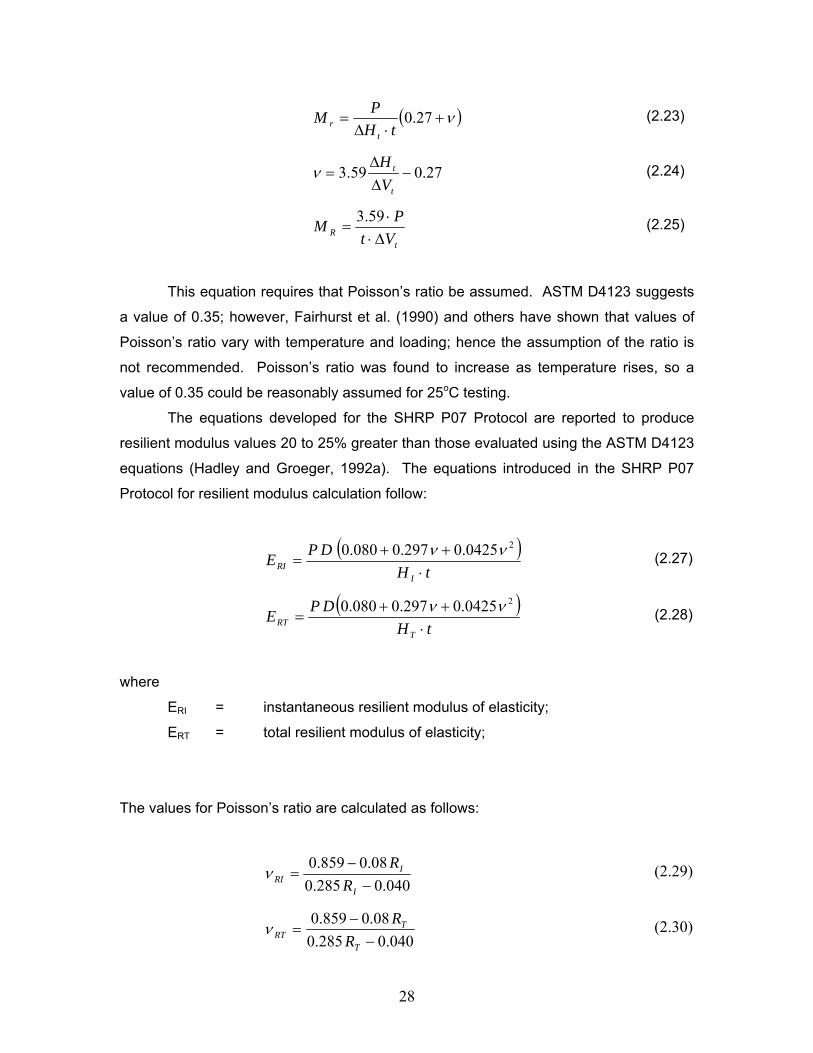
This equation requires that Poisson’s ratio be assumed. ASTM D4123 suggests

a value of 0.35; however, Fairhurst et al. (1990) and others have shown that values of

Poisson’s ratio vary with temperature and loading; hence the assumption of the ratio is

not recommended. Poisson’s ratio was found to increase as temperature rises, so a

value of 0.35 could be reasonably assumed for 25oC testing.

The equations developed for the SHRP P07 Protocol are reported to produce

resilient modulus values 20 to 25% greater than those evaluated using the ASTM D4123

equations (Hadley and Groeger, 1992a). The equations introduced in the SHRP P07

Protocol for resilient modulus calculation follow:

( )tH

DPEI

RI ⋅++

=20425.0297.0080.0 νν (2.27)

( )tH

DPET

RT ⋅++

=20425.0297.0080.0 νν (2.28)

where

ERI = instantaneous resilient modulus of elasticity;

ERT = total resilient modulus of elasticity;

The values for Poisson’s ratio are calculated as follows:

040.0285.0

08.0859.0−

−=

I

IRI R

Rν (2.29)

040.0285.0

08.0859.0−

−=

T

TRT R

Rν (2.30)

29

I

II H

VR = (2.31)

T

TT H

VR = (2.32)

where

VI = instantaneous recoverable vertical deformation; and

VT = total recoverable vertical deformation.

Another research effort, by Fairhurst et al. (1990), evaluated the MTS test system

for the determination of resilient modulus. Results indicated that the MR decreases and

Poisson’s ratio increases as the testing temperature rises. In addition, the resilient

modulus was found to increase with cycle frequency. Possibly, this increase occurred

because the decreased recovery times caused by increased test frequencies resulted in

an accumulation of strain in the specimen. It was found that after a 90° rotation of the

specimen, the resilient modulus was lower and Poisson’s ratio slightly higher that the

results in the 0° position. This could have occurred due to slight internal damage during

testing in the 0° position. The increase in Poisson’s ratio may be caused by a

redistribution of stresses around the damaged area, which results in greater specimen

deformations during testing at the 90° position.

2.4.2 Roque and Buttlar’s Indirect Tension Specimen Analysis

Roque and Buttlar’s indirect tension specimen analysis is based on the

conception that plane stress conditions from the IDT test traditionally assumed to

determine moduli do not actually apply for standard size specimens (Mamlouk and

Sarofim, 1988). Therefore, moduli determined using measured vertical deformation can

be significantly erroneous (Heinicke and Vinson, 1988). Using three-dimensional finite

element (FE) analysis, Roque and Buttlar (1992) showed that the horizontal stress along

the specimen thickness is not uniform. They found that the plane stress assumption is

valid only for specimen thicknesses less than 25-mm. For thicknesses of 60-mm and

more, non-uniformity in the stress, measured along the specimen thickness, will cause

irregular bulging on the x and y axes and will, therefore, affect measurements obtained

from the surface mounted sensors, causing them to rotate (Figure 2-2, after Roque and

Buttlar, 1992).

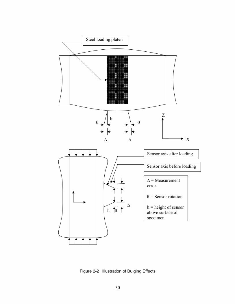
30

Figure 2-2 Illustration of Bulging Effects

h∆

θ

Sensor axis before loading

Sensor axis after loading

∆ = Measurement error θ = Sensor rotation h = height of sensor above surface of specimen

Z h

θ

Steel loading platen

∆ ∆

θ

X

31

The extent of bulging in the specimen was found to depend upon Poisson’s ratio.

Analyses were performed assuming a modulus of 1,380 MPa and three values of

Poisson’s ratio: 0.20, 0.35, and 0.45. For specimen bulging effect, correction factors,

based on the specimens’ diameter to thickness ratio, obtained from the three-

dimensional FE solution were developed to adjust for the measured deformations along

both axes. These correction factors permit researchers to approach the three-

dimensional problem using two-dimensional analysis. Since the extent of bulging

depends on Poisson’s ratio, which is not known a priori, the analysis involves an iterative

procedure, which should be valid for both 100- and 150-mm diameter specimens.

The analysis applies only for a gauge-length-to-diameter ratio of 1:4 and when

the height of the extensiometers is 6.25-mm from the specimen surface. Tensile

deformation is considered to be positive; compressive deformation is negative. The

Roque and Buttlar data analysis was used in this research for the following reasons:

• The deflection measurement devices used in the research are similar to the ones

the method was developed for,

• The method takes into account the deviation from the plane stress assumptions,

• The method allows the calculation of Poisson’s ratio from deflection

measurements, and,

• The method is valid for any specimen size, which is the case in this research

where 100- and 150-mm diameter specimens were tested.

2.4.3 Three Dimensional Solution for the Indirect Tensile Test

The following three-dimensional solution for the indirect tensile test is based on

the two-dimensional plane stress solution presented by Wijk (1978), wherein the latter is

a “special case” of the three-dimensional one with stresses σz, τxz, and τyz approaching

zero.

If the potential stress function of the two-dimensional problem is ϕ(x, y), then the

normal stresses are σx(x, y) and σy(x, y) in the following format (Wijk 1978):

2

2 ),(y

yxx ∂

∂=

ϕσ (2.33)

32

2

2 ),(x

yxy ∂

∂=

ϕσ (2.34)

Three-dimensional solutions may be obtained for the IDT with the following

observations:

σz(x, y, z)= τzx(x, y, z)= τzy(x, y, z)=0 (2.35)

Based on this observation, Wijk (1978) derived the following equations for stresses:

2

2 ),,(),(),,(y

zyxyxzyx xx ∂∆∂

+=ϕσσ (2.36)

2

2 ),,(),(),,(x

zyxyxzyx yy ∂∆∂

+=ϕσσ (2.37)

),()1/1(2

),,( 2

2

2

22

yxyx

zzyx ϕν

ϕ⎭⎬⎫

⎩⎨⎧

∂∂

+∂∂

+−=∆ (2.38)

where ν is Poisson’s ratio.

Input equation (2.38) into equations (2.36) and (2.37) result in the following:

),()1/1(2

),(),,( 4

2

22

22

yxyyx

zyxzyx xx ϕν

σσ⎭⎬⎫

⎩⎨⎧

∂∂

+∂∂∂

+−= (2.39)

),()1/1(2

),(),,( 22

2

4

22

yxyxx

zyxzyx yy ϕν

σσ⎭⎬⎫

⎩⎨⎧

∂∂∂

+∂∂

+−= (2.40)

The normal and shear stresses at the faces of an indirect tensile specimen are

zero for both the two-dimensional and three-dimensional cases. The stress-strain

relationship in a three-dimensional problem is therefore the same as that in a two-

dimensional one:

33

Eyxx /)( νσσε −= (2.41)

Exyy /)( νσσε −= (2.42)

where E is Young’s modulus.

The three-dimensional stresses σx and σy from Equations (2.39) and (2.40) are

input into Equations (2.41) and (2.42), thus obtaining the following general expressions

of three-dimensional strain distribution:

Eyxyxx

zyx

yxyyx

zyx

y

xx

/)],()1/1(2

),([

),()1/1(2

),(

22

2

4

22

4

2

22

22

ϕν

σν

ϕν

σε

⎭⎬⎫

⎩⎨⎧

∂∂∂

+∂∂

+−

−⎭⎬⎫

⎩⎨⎧

∂∂

+∂∂∂

+−=

(2.43)

Eyxyyx

zyx

yxyxx

zyx

x

yy

/)],()1/1(2

),([

),()1/1(2

),(

4

2

22

22

22

2

4

22

ϕν

σν

ϕν

σε

⎭⎬⎫

⎩⎨⎧

∂∂

+∂∂∂

+−

−⎭⎬⎫

⎩⎨⎧

∂∂∂

+∂∂

+−=

(2.44)

Horizontal and vertical displacements are obtained by integrating the strains

along the gauge length. The solutions for the vertical and horizontal displacements are

functions of the specimen diameter, and the gauge length as follows:

)1()( 22

42

321

νννν

++++

=Et

dCCCCPU (2.45)

)1()( 22

82

765

νννν

++++

=Et

dCCCCPV (2.46)

34

2.5 Summary

Pavement design requires the characterization of the paving materials. Hot mix

asphalt resilient modulus is an important material property that needs to be determined

for pavement design. The IDT test has become the most widely used laboratory test to

determine the resilient modulus of HMA. However the resilient modulus depends on

many parameters. In addition, data analysis of the IDT test is somewhat complicated.

Significant effort has been directed towards determining the state of stress in the IDT

specimen (Roque and Buttlar, 1992; Kim et al., 2002). The Roque and Buttlar data

analysis was developed for a testing system similar to the one used in this research and

seems very promising since it takes into account three dimensional effects. The next

chapter presents the research approach undertaken in this study.

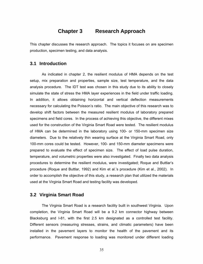
35

Chapter 3 Research Approach

This chapter discusses the research approach. The topics it focuses on are specimen

production, specimen testing, and data analysis.

3.1 Introduction

As indicated in chapter 2, the resilient modulus of HMA depends on the test

setup, mix preparation and properties, sample size, test temperature, and the data

analysis procedure. The IDT test was chosen in this study due to its ability to closely

simulate the state of stress the HMA layer experiences in the field under traffic loading.

In addition, it allows obtaining horizontal and vertical deflection measurements

necessary for calculating the Poisson’s ratio. The main objective of this research was to

develop shift factors between the measured resilient modulus of laboratory prepared

specimens and field cores. In the process of achieving this objective, the different mixes

used for the construction of the Virginia Smart Road were tested. The resilient modulus

of HMA can be determined in the laboratory using 100- or 150-mm specimen size

diameters. Due to the relatively thin wearing surface at the Virginia Smart Road, only

100-mm cores could be tested. However, 100- and 150-mm diameter specimens were

prepared to evaluate the effect of specimen size. The effect of load pulse duration,

temperature, and volumetric properties were also investigated. Finally two data analysis

procedures to determine the resilient modulus, were investigated; Roque and Buttlar’s

procedure (Roque and Buttlar, 1992) and Kim et al.’s procedure (Kim et al., 2002). In

order to accomplish the objective of this study, a research plan that utilized the materials

used at the Virginia Smart Road and testing facility was developed.

3.2 Virginia Smart Road

The Virginia Smart Road is a research facility built in southwest Virginia. Upon

completion, the Virginia Smart Road will be a 9.2 km connector highway between

Blacksburg and I-81, with the first 2.5 km designated as a controlled test facility.

Different sensors (measuring stresses, strains, and climatic parameters) have been

installed in the pavement layers to monitor the health of the pavement and its

performance. Pavement response to loading was monitored under different loading

36

conditions, truck tire pressure, temperature, and driving speed. The vertical

compressive stress pulse induced by a moving truck and by FWD testing was

determined at different locations. The average pulse width of the moving truck was

determined at 8, 24, 40, and 72 km/h.

The flexible pavement part of the Virginia Smart Road test facility includes 12 heavily

instrumented flexible pavement sections. Section length varies between 76 and 117 m.

Seven of the 12 sections are located on a fill, while the remaining five sections are

located on a cut. Different layers are used in each section (all designations and HMA

designs are in accordance with the Virginia Department of Transportation

Specifications). The different pavement layers are as follows:

• Wearing surface: Seven types of HMA wearing surface are used (SM-9.5A, SM-

9.5A with high laboratory compaction, SM-9.5D, SM-9.5E, SM-12.5D, and an

open-graded friction course [OGFC]). Five of these seven mixes are

SuperpaveTM. All of the mixes, with the exception of the OGFC, were constructed

at 38-mm-thick. The OGFC was constructed at 19-mm-thick.

• Intermediate HMA layer: BM-25.0 at different thicknesses ranging from 100 to

244 mm.

• Three sections have the SuperpaveTM SM9.5A fine mix placed under the BM-

25.0 to examine the benefits of such a design on reducing fatigue cracking.

• Open-graded drainage layer [OGDL]: Out of the 12 sections, three sections were

built without the OGDL. Seven sections are treated with asphalt cement and two

are treated with Portland cement. The thickness of this layer was kept constant

at 75 mm throughout the project.

• Cement stabilized subbase: 21-A cement-stabilized layer used in 10 sections at a

thickness of 150 mm.

• Subbase layer: 21-B aggregate layer was placed over the subgrade at different

thickness with and without a geosynthetic.

The structural configuration of the Virginia Smart Road is presented in figure 3.1. The

laboratory-measured resilient moduli can be used to calculate stresses and strains in

using the layered elastic theory and then compare the obtained values to field

measurements obtained from truck testing. Mix properties other than the resilient

modulus that are being determined at the Virginia Smart Road are creep and fatigue

characteristics.

37

Figure 3-1 Structural configuration of Virginia Smart Road.

3.3 Hot Mix Asphalt Preparation

The seven different mixes that were placed at the Virginia Smart Road are

presented in Table 3.1. Materials for this study were provided either directly from the

Geocomposite Membrane

A-D J K L E F G H I

A - D E F G H I J K LOGFC* HMA

Wearing Surface - - - - - - - 19 -

HMA Wearing Surface 38 38 38 38 38 38 38 19 38

HMA Base 150 225 150 100 100 100 225 244 150HMA Surface

(placed as base) - - - 50 50 50 - - -

Asphalt Stabilized OGDL** 75 - - - 75 75 75 - -Cement Stabilized OGDL - - - - - - - 75 75

Cement Stabilized Aggregate Base 150 150 150 150 150 150 - - 150

21B Aggregate Base 175 75 150 150 75 75 75 150 75* OGFC - Open Graded Friction Course** OGDL - Open Graded Drainage Layer

Material Section / Thickness (mm)

38

Virginia Smart Road, in the form of road cores or loose bagged mixture samples

collected during construction, or were produced from raw materials to meet either

volumetric criteria determined from road cores or to meet design specifications. All raw

materials used for production of specimens were obtained from the source utilized

during construction. Practices recommended by the Virginia Department of

Transportation and in accordance with Superpave protocol were implemented in

specimen preparation.

Table 3-1 Mixture characteristics at the Virginia Smart Road

Section HMA Wearing Surface Characteristics

A SM-12.5D 12.5mm nominal maximum aggregate size

PG 70-22 binder

B, E – H, J SM-9.5D 9.5mm nominal maximum aggregate size

PG 70-22 binder

C SM-9.5E 9.5mm nominal maximum aggregate size

PG 76-22 binder

D, I SM-9.5A

9.5mm nominal maximum aggregate size

PG 64-22 binder

Section I designed with high lab compaction

K OGFC 12.5mm nominal maximum aggregate size

PG 76-22 binder

L SMA-12.5 12.5mm nominal maximum aggregate size

PG 76-22 binder

3.3.1 Specimen Designation and Characteristics

Three specimen types were produced in two different sizes; 100-mm diameter

specimens and 63.5-mm thick and 150-mm diameter specimens and 76.2-mm thick. A

fourth specimen type was obtained from the Virginia Smart Road in form of 100-mm

diameter field cores. The thickness of the field cores was controlled by the thickness of

the constructed HMA layer. The four specimen types are divided into the following

categories:

39

• Field/field (F/F): field cores from the Virginia Smart Road, only available in 100-

mm diameter. Field core thickness is controlled by the wearing thickness at the

Virginia Smart Road and varied between 37 and 50 mm;

• Field/lab (F/L): specimens compacted in the laboratory from loose mixtures

samples obtained from the field at the time of construction;

• Lab/lab (L/L): specimens produced and compacted in the laboratory using

volumetric results from field specimens; and

• Design/lab (D/L): specimens produced and compacted in the laboratory

according to design specifications.

The analysis of volumetric properties was performed for all mixtures. It included

specimen bulk specific gravity and compaction densification curves, mixture maximum

theoretical specific gravity (Rice), aggregate gradation, and asphalt content

measurements for the four different types of mixes. The results are presented in

Appendices A and B. The Summary of the tests specimens for resilient modulus

evaluation is presented in Table 3-2.

Table 3-2 Number of Tested Specimens

Section Mixture F/F F/L L/L D/L* a a b a b a b A SM12.5D 2 3 2 3 2 6 2 B SM-9.5D 2 3 2 3 2 6 2 C SM-9.5E 2 3 2 3 2 6 2 D SM-9.5A 2 3 2 3 2 6 2 E SM-9.5D 2 3 2 3 2 F SM-9.5D 2 3 2 G SM-9.5D 2 3 2 H SM-9.5D 2 3 2

Same as E Same as B

I SM-9.5A* 2 3 2 3 2 6 2 J SM-9.5D 2 3 2 3 2 Same as B K OGFC Not tested L SM-12.5 2 3 2 3 2 6 2

D/L* 3 specimens tested at 0.1 sec load pulse and 3 specimens tested at 0.03 sec

load pulse

a 100-mm diameter specimens with 63-mm thickness

b 150-mm diameter specimens with 75-mm thickness

40

3.3.2 Specimen Preparation

Field/Field Specimens

F/F specimens consist of cores obtained from the Virginia Smart Road wearing

surface. After core extraction, the wearing surface was separated from the base mix

(BM). The extracted samples’ surfaces had to be treated so that they are smooth

enough to mount the extensiometers. The specimen thickness was recorded as the

average of three measurements taken at 120o intervals.

Field/Lab Specimens

Field/Lab mixes were collected during the construction of the Virginia Smart

Road. Samples were heated to be brought up to compaction temperature. This

procedure was performed in less than an hour to prevent specimen aging. The

specimens were then compacted using a troxler gyratory compactor. The compaction

temperature ranged between 135 and 144oC. The specimens volumetric properties

were then taken before they were cut to the specified thickness (63.5- and 76.2-mm for

100- and 150-mm specimens respectively) to be tested.

Lab/Lab Specimens

Lab/Lab mixes were produced in the laboratory to replicate F/L mixes.

Aggregate gradation and asphalt content were determined by from F/L mixes, using the

ignition oven for asphalt content determination. Lab/Lab gradations were designed to

replicate as closely as possible F/L gradations by mixing the proper amount of the

different aggregate types used for the construction of the Virginia Smart Road. The

proper amount of asphalt binder was then added to the aggregate for mixing. The

mixing temperature ranged between 135 and 170oC. The procedure for compaction and

final sample preparation was the same as for F/L specimens.

Design/Lab Specimens

The procedure for preparing D/L specimens was the same as the one for L/L

specimens except that the aggregate gradation and asphalt content are determined from

the design sheets.

41

3.3.3 Laboratory Compaction

The effect of mix preparation and construction practices can be minimized with

better quality control. The effect of compaction can only be controlled when the

compaction method used in the laboratory simulates field compaction. However, this

could be difficult to achieve due to the difference between pavement construction and

laboratory prepared specimens. Laboratory compacted specimens are designated as

F/L, L/L, and D/L. In this case, only differences in mix preparation between the

laboratory and the mixing plant were considered. Gyratory compaction has been shown

to be the method of compaction that most accurately replicates field compaction. The

gyratory compactor used is the Troxler compactor, in accordance with AASHTO TP-4

(Table 3-2).

Figure 3-2 Troxler Gyratory Compactor.

The compaction pressure used is 600 KPa at an angle of 1.25o. The number of

gyrations is as specified in Table 3-3. The specimens were compacted at N Design.

42

Table 3-3 Number of Gyrations for each Mix

Number of Gyrations Section

HMA Wearing

Surface N Design N Initial N max

A SM-12.5D 75 7 115

B, E – H, J SM-9.5D 75 7 115

C SM-9.5E 75 7 115

D, I SM-9.5A 65 7 100

K OGFC Not Tested

L SMA-12.5

Prior to compaction, the HMA and the mold were heated to the specified compaction

temperature. When compaction was completed, the specimens were allowed to cool

down before being extracted from the mold, which would reduce the possibility of

inducing residual stresses on the specimen sides. The volumetric properties were then

measured before cutting the samples to the specified thickness for testing.

3.4 Specimen Testing

As indicated in chapter 2, the IDT setup was chosen in this research mainly due to

its relative simplicity in comparison to the triaxial setup and its ability to simulate the

state of stress that is present in the field.

AASHTO TP9-96 provides the standard test method for IDT test. The test

procedure is based on ASTM D4123. One difference between the AASHTO setup and

the one used in this study is the loading frame which consists of four columns in

AASHTO TP9-96 whereas this study uses a two columns loading frame. Another

difference is that AASHTO TP9-96 uses mounted LVDTs for deflection measurements

whereas in this study spring mounted extensiometers were used as shown in Figure 3.3.

Bracket mounts are glued on both specimen faces as shown in Figure 3.3a. The

distance between the mounts is 25.4- and 38.1-mm for 100- and 150-mm specimens,

respectively. Then the brackets are fixed on the mounts as shown in Figure 3.3b. Two

sets of brackets were used; one for 100-mm specimens and another for 150-mm

specimens. Two sets were required since the same set of extensiometers is used for

both diameter sizes while the gauge length is different. Finally, the exstensiometers are

43

mounted on the brackets (Figure 3.3c). The specimen diameter to gauge length ratio is

the same for both specimen sizes. The gauge length is set at 25.4-mm for 100-mm

diameter specimens as specified in AASHTO TP9-96. The gauge length for the 150-mm

diameter specimens is 38.1-mm. The gauge length chosen is important to minimize the

possibility of placing the gauge in a zone primarily influenced by a single aggregate. A

minimum of 25.4 mm gauge length is, therefore, required for 100-mm diameter

specimens and was used by Roque and Buttlar (1992), Ruth and Maxfield (1977),

Anderson and Hussein (1990), and Hugo and Nachenius (1989). Also, a gauge of 25.4-

mm for 100-mm specimens and 38.1-mm for 150mm specimens will ensure that

deflections are measured over an area of relatively uniform stress distribution as

suggested by Roque and Buttlar (1992).

a) Glued mount b) Brackets

c) Extensiometers

Figure 3-3 Extensiometer Mounting

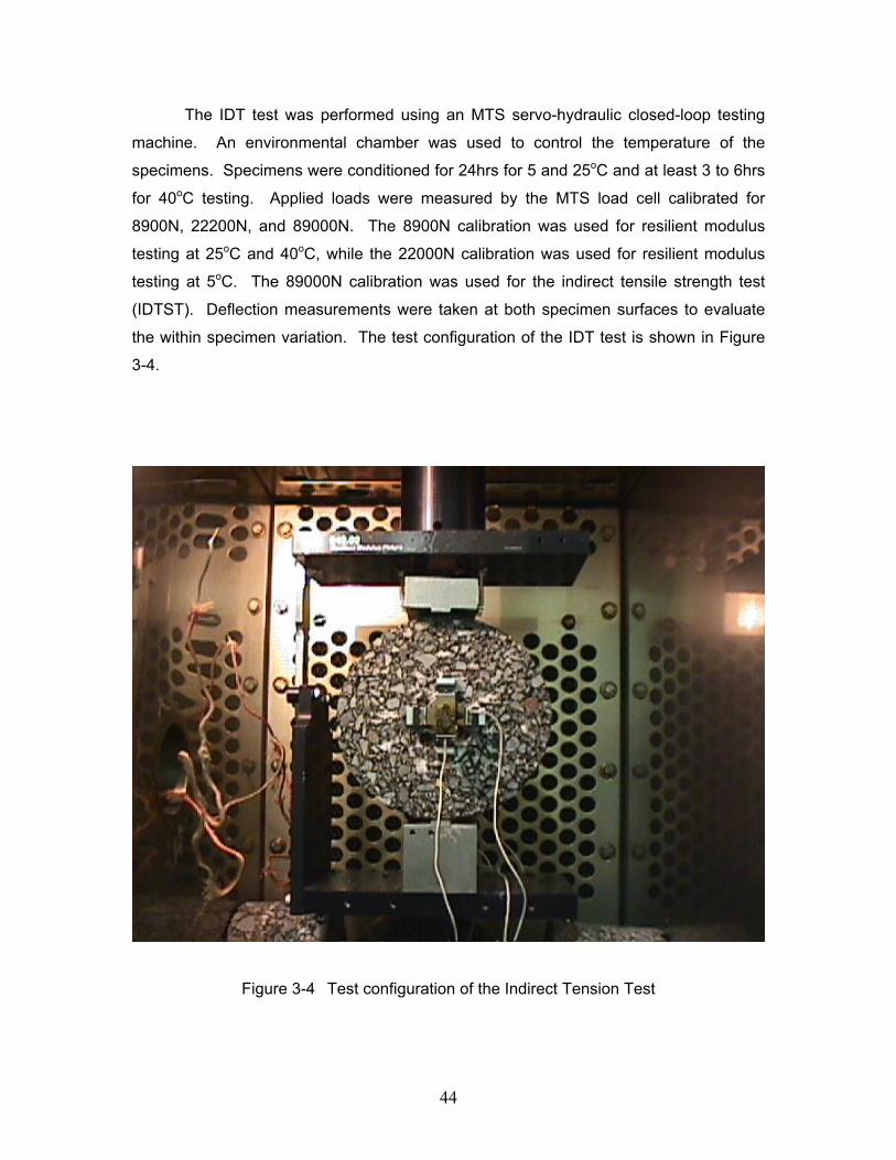
44

The IDT test was performed using an MTS servo-hydraulic closed-loop testing

machine. An environmental chamber was used to control the temperature of the

specimens. Specimens were conditioned for 24hrs for 5 and 25oC and at least 3 to 6hrs

for 40oC testing. Applied loads were measured by the MTS load cell calibrated for

8900N, 22200N, and 89000N. The 8900N calibration was used for resilient modulus

testing at 25oC and 40oC, while the 22000N calibration was used for resilient modulus

testing at 5oC. The 89000N calibration was used for the indirect tensile strength test

(IDTST). Deflection measurements were taken at both specimen surfaces to evaluate

the within specimen variation. The test configuration of the IDT test is shown in Figure

3-4.

Figure 3-4 Test configuration of the Indirect Tension Test

45

3.4.1 Loading

The applied load was selected in a way to limit the strain between 150 and 500

microstrain. The upper limit of 500 microstrain was set to prevent specimen damage as

recommended by Roque and Buttlar (1994), whereas the lower limit of 150 microstrain is

set to obtain measurements much higher than the LVDTs’ sensitivity. In this study, the

150 microstrain criterion was used after it was found that the signal to noise ratio of the

extensiometers, at this range of strains, was very high. Hence, the applied load varied

between mixes design and specimen sizes. The load used is a haversine load of 0.1

sec pulse duration and 0.9 sec rest period for all the specimens. A second set of D/L

specimens was tested at a load of 0.03 sec pulse duration and 0.97 rest period as

suggested by Loulizi et al. (2002). Since the load was not known a priori, many tests

were performed on the first specimen of each section to define the appropriate loading.

The initial applied load was relatively small to prevent damaging the specimen. The

specimen was allowed to recover for a period of 30mins before it was tested again under

a different loading. The load at which the measured horizontal and vertical deformations

fell in the range of 150 and 500 microstrain was the load used to test the rest of the

specimens. This same procedure was repeated for each mix at the three different

temperatures (5, 25, and 40oC). The final loads used for testing are presented in

Chapter 4.

3.4.2 Testing and Data Collection

The IDT test for the resilient modulus was conducted at 100 cycles for all testing

temperatures. After 100 cycles, the accumulated plastic strain per cycle becomes

negligible. The 100 conditioning cycles simulate the consolidation that occurs in

pavements when it is opened for traffic. Deflection and load readings were recorded for

the last 5 cycles of the test at 0.0048828 sec intervals. The readings were averaged to

determine the resilient modulus and Poisson’s ratio. The calculated resilient modulus

variation in any two loading cycles has to be lower than 5% for test results acceptance.

Two resilient modulus and Poisson’s ratio values were determined for every specimen;

one at each specimen’s surface. An example of the collected data is presented in figure

3.5.

46

Load vs. T ime

1.68E+00

6.68E+00

1.17E+01

1.67E+01

2.17E+01

124.34 124.84 125.34 125.84 126.34 126.84 127.34 127.84 128.34 128.84 129.34

Time (Sec)

Load

(kN

)

(a) Applied Load

Vertical Deformation vs. T ime

3.57E-013.59E-013.61E-013.63E-013.65E-013.67E-01

124.34 124.84 125.34 125.84 126.34 126.84 127.34 127.84 128.34 128.84 129.34

Time (Sec)

Vert

ical

Def

orm

atio

n (m

m)

(b) Measured Vertical Deformation

Horizontal Deformation vs. T ime

2.83E-012.84E-012.85E-012.86E-012.87E-012.88E-01

124.34 124.84 125.34 125.84 126.34 126.84 127.34 127.84 128.34 128.84 129.34

Time (Sec)

Hor

izon

tal

Def

orm

atio

n (m

m)

(c) Measured Horizontal Deformation

Figure 3-5 Collected Data for Resilient Modulus Testing

47

The IDT test for resilient modulus is run in such a way that 10% of the maximum

applied load is maintained during the rest period. This is done to ensure contact

between the loading plates and the specimen throughout the test which will reduce the

risk of specimen movement during loading and unloading. The horizontal and vertical

deformations are taken as the difference between the maximum and the minimum

readings of each of the vertical and horizontal extensiometers, respectively.

3.4.3 Indirect Tensile Strength Test

After the resilient modulus test was performed at the three different temperatures

of 5, 25, and 40oC, specimens were allowed to recover for a period of 24 hrs before they

were tested for their indirect tensile strength. The indirect tensile strength test was

performed at a temperature of 25oC. The test was performed to compare the applied

load for resilient modulus testing to the indirect tensile strength, since this is the

procedure suggested by ASTM D 4123. A load was applied to the specimen at a

constant crosshead rate; it is desirable to have a constant strain rate input. However,

since the strain is calculated from extensiometer measurements and in order to prevent

damaging them, the extensiometers had to be removed from the specimen surfaces,

and a constant crosshead rate of 50.1 mm/min was used. Failure is detected when the

applied load drops to 75% of the maximum applied load. Since the extensiometers are

removed, it is not possible to calculate Poisson’s ratio during testing. Hence, the stress

in the specimen is calculated using Hondro’s plane stress solution. The indirect tensile

strength results are presented in Appendix C.

3.5 Resilient Modulus Calculations

As presented in Chapter 2, many methods were developed by different

researchers to calculate the resilient modulus from indirect tensile testing. The Roque

and Buttlar (1992) method and Kim et al. method (2002) were used in this research for

the following reasons:

• The analyses take into account three-dimensional effects

• The analyses allows for determining Poisson’s ratio instead of assuming one

• The analyses take into account the specimen dimensions (thickness and

diameter)

• The Roque and Buttlar analysis was verified by finite element analysis

48

3.5.1 Roque and Buttlar’s Procedure for Resilient Modulus Calculation

The Roque and Buttlar’s procedure account for the effect of specimen bulging.

Specimen bulging would cause the externally mounted extensiometers to rotate and,

therefore, affect the vertical and horizontal deflection readings. The extent of bulging is

dependent on the Poisson’s ratio (Roque and Buttlar, 1992). Since Poisson’s ratio is not

known a priori, the analysis involves an iterative procedure. The determination of the

resilient modulus and Poisson’s ratio for an IDT test specimen based on the Roque and

Buttlar data analysis is as follows (Roque and Buttlar, 1992):

1. Assume Poisson’s ratio

2. Correct for horizontal deformation to account for bulging effect as follows:

⎭⎬⎫

⎩⎨⎧

⎟⎟⎠

⎞⎜⎜⎝

⎛−−=

stdB t

tCx

05.012.001.1 ν (3.1)

where,

xBC = correction factor applied for the measured horizontal deformation

to correct for specimen bulging = H/HM,

H = corrected horizontal deformation,

HM = measured horizontal deformation,

t = measured specimen thickness,

tstd = standard specimen thickness (62.5mm for 100mm specimens),

HM = measured horizontal deformation, and

ν = Poisson’s ratio.

3. Correct vertical deformation to account for bulging effect as follows:

( )ν128.0994.0 −=yBC (3.2)

where,

yBC = correction factor applied to the measured vertical deformation to

correct for specimen bulging = Y/YM ;

49

Y = corrected vertical deformation; and

YM = measured vertical deformation.

4. Convert the average strains measured by the gages to point strains. The relationship

between average and point strain is independent of Poisson’s ratio. The horizontal and

vertical strains are then calculated as follows:

xx BCTR C

GLH

×= 07.1ε (horizontal strain) (3.3)

yy BCTR C

GLY

×= 98.0ε (vertical strain) (3.4)

where,

GL = gage length, mm;

H = horizontal deformation, mm; and

Y = vertical deformation, mm.

5. Correct for horizontal and vertical point stress at the center of the specimen:

TxCTRstd

x Cdt

PCORR ×

=π

σ 2 (3.5)

TyCTRstd

y Cdt

PCORR ×

=π

σ 6 (3.6)

where,

CORRxσ = corrected horizontal point stress;

CORRyσ = corrected vertical point stress;

TxCTRC = correction factor applied to the horizontal point stress; and

TyCTRC = correction factor applied to the vertical point stress;

The correction factor for both the horizontal and the vertical stress are given in Table

3-4.

50

Table 3-4 Correction Factors for Horizontal and Vertical Stress

Diameter to Thickness Ratio

D=100 or 150-mm ν 0.167 0.333 0.500 0.625 0.750

0.20 0.9471 0.9773 1.0251 1.0696 1.1040

0.35 0.9561 1.0007 1.0871 1.1682 1.2321 TxCTRC

0.45 0.9597 1.0087 1.1213 1.2307 1.3171

0.20 -0.9648 -0.9754 -0.9743 -0.9693 -0.9611

0.35 -0.9732 -0.9888 -0.9844 -0.9710 -0.9538 TyCTRC

0.45 -0.9788 -0.9971 -0.9864 -0.9646 -0.9395

6. Determine Poisson’s ratio as follows:

CORR

y

x

CORR

CORR

y

x

CORR

xCTR

CTRy

yCTR

CTRx

σεε

σ

σεε

σ

ν

⎟⎟

⎠

⎞

⎜⎜

⎝

⎛−

⎟⎟

⎠

⎞

⎜⎜

⎝

⎛−

= (3.7)

If Poisson’s ratio calculated using equation (3.7) differs by more than 0.01 with

assumed Poisson’s ratio in step 1 then replace the new value in step 1 and repeat step 2

to 6, otherwise continue to step 7

7. The HMA resilient modulus is determined as follows:

( )CORRCORR

x

yxCTR

RM νσσε

−=1

(3.8)

3.5.2 Three-Dimensional Solution

Wijk (1978) suggested constructing the solution of a three-dimensional problem

using the solution to a two-dimensional problem. A three-dimensional solution to the

indirect tensile test can therefore be constructed based on the two-dimensional plane

stress solution where the stresses σz, τxz, and τyz vanish.

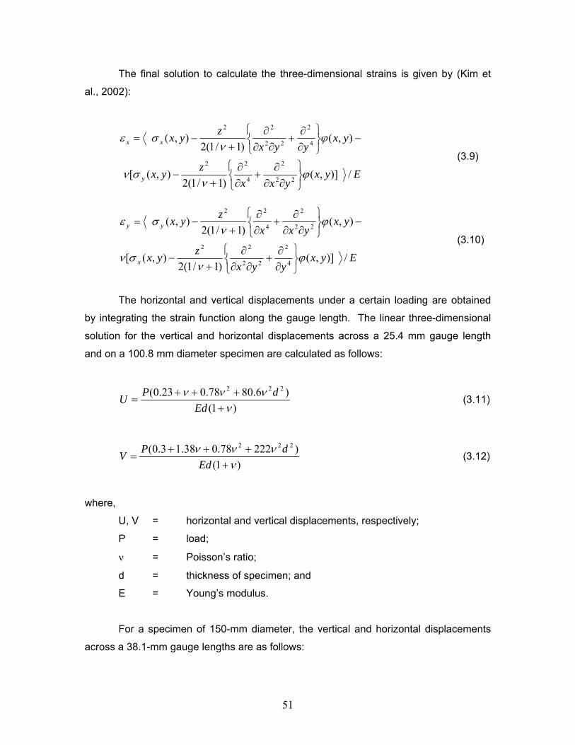
51

The final solution to calculate the three-dimensional strains is given by (Kim et

al., 2002):

Eyxyxx

zyx

yxyyx

zyx

y

xx

/)],()1/1(2

),([

),()1/1(2

),(

22

2

4

22

4

2

22

22

ϕν

σν

ϕν

σε

⎭⎬⎫

⎩⎨⎧

∂∂∂

+∂∂

+−

−⎭⎬⎫

⎩⎨⎧

∂∂

+∂∂∂

+−=

(3.9)

Eyxyyx

zyx

yxyxx

zyx

x

yy

/)],()1/1(2

),([

),()1/1(2

),(

4

2

22

22

22

2

4

22

ϕν

σν

ϕν

σε

⎭⎬⎫

⎩⎨⎧

∂∂

+∂∂∂

+−

−⎭⎬⎫

⎩⎨⎧

∂∂∂

+∂∂

+−=

(3.10)

The horizontal and vertical displacements under a certain loading are obtained

by integrating the strain function along the gauge length. The linear three-dimensional

solution for the vertical and horizontal displacements across a 25.4 mm gauge length

and on a 100.8 mm diameter specimen are calculated as follows:

)1(

)6.8078.023.0( 222

νννν

++++

=Ed

dPU (3.11)

)1()22278.038.13.0( 222

νννν

++++

=Ed

dPV (3.12)

where,

U, V = horizontal and vertical displacements, respectively;

P = load;

ν = Poisson’s ratio;

d = thickness of specimen; and

E = Young’s modulus.

For a specimen of 150-mm diameter, the vertical and horizontal displacements

across a 38.1-mm gauge lengths are as follows:

52

)1()81.30588.0773.018.0( 222

νννν

++++

=Ed

dPU (3.13)

)1()5.4868.089.021.0( 222

νννν

++++

=Ed

dPV (3.14)

The two unknwons that need to be determined are Poisson’s ratio and the

resilient modulus. In the case of a 100-mm diameter specimen, equations 3.11 and 3.12

can be rewritten as follows:

)1()6.8078.023.0( 222

νννν

++++

=Ud

dPE (3.15)

)1()22278.038.13.0( 222

νννν

++++

=Vd

dPE (3.16)

Similarly for the case of a 150-mm diameter specimen equations 3.13 and 3.14

are rewritten as follows:

)1()81.30588.0773.018.0( 222

νννν

++++

=Ud

dPE (3.17)

)1()5.4868.089.021.0( 222

νννν

++++

=Vd

dPE (3.18)

Combining equations 3.15 through 3.18, an expression to calculate Poisson’s

ratio results in the following:

UV

dd

=++++++

)6.8078.023.0()6.8078.023.0(

222

222

νννννν (3.19)

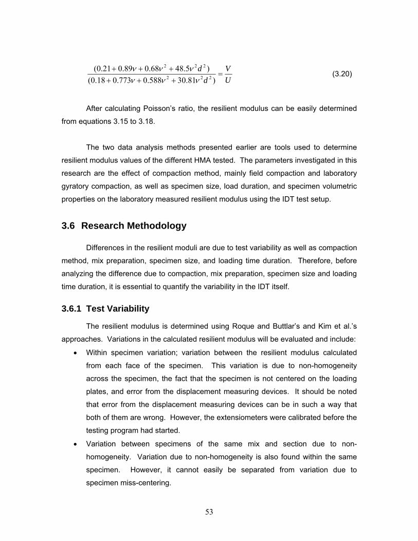
53

UV

dd

=++++++

)81.30588.0773.018.0()5.4868.089.021.0(222

222

νννννν (3.20)

After calculating Poisson’s ratio, the resilient modulus can be easily determined

from equations 3.15 to 3.18.

The two data analysis methods presented earlier are tools used to determine

resilient modulus values of the different HMA tested. The parameters investigated in this

research are the effect of compaction method, mainly field compaction and laboratory

gyratory compaction, as well as specimen size, load duration, and specimen volumetric

properties on the laboratory measured resilient modulus using the IDT test setup.

3.6 Research Methodology

Differences in the resilient moduli are due to test variability as well as compaction

method, mix preparation, specimen size, and loading time duration. Therefore, before

analyzing the difference due to compaction, mix preparation, specimen size and loading

time duration, it is essential to quantify the variability in the IDT itself.

3.6.1 Test Variability

The resilient modulus is determined using Roque and Buttlar’s and Kim et al.’s

approaches. Variations in the calculated resilient modulus will be evaluated and include:

• Within specimen variation; variation between the resilient modulus calculated

from each face of the specimen. This variation is due to non-homogeneity

across the specimen, the fact that the specimen is not centered on the loading

plates, and error from the displacement measuring devices. It should be noted

that error from the displacement measuring devices can be in such a way that

both of them are wrong. However, the extensiometers were calibrated before the

testing program had started.

• Variation between specimens of the same mix and section due to non-

homogeneity. Variation due to non-homogeneity is also found within the same

specimen. However, it cannot easily be separated from variation due to

specimen miss-centering.

54

3.6.2 Shift Factors

Shift factors are developed for the method of compaction, the specimen size, and

the loading time duration. The compaction shift factor reflects the difference in the

measured resilient modulus from F/F and F/L specimens. Since these specimens differ

only in the way they were compacted, any difference in the measured resilient moduli

will be due to difference in compaction. To validate the effect of compaction on the

measured resilient moduli, two volumetric properties are investigated: sample specific

gravity and air void content.

The state of stress in the IDT specimen as well as deflection measurements

taken at the specimens’ surfaces should result in the same resilient modulus for either

100- or 150-mm diameter specimens. This is not the case for Hondro’s plane stress

solution. Roque and Buttlar (1992) developed correction factors for stress and strain in

the IDT specimen. These correction factors are applied to Hondro’s solution and are

independent of the specimen size. The ability for these correction factors to be able to

take into account the specimen size and therefore, result in the same resilient modulus

results for 100- and 150-mm diameter specimens is evaluated. A specimen size shift

factor is developed to take into account any variation between the 100- and 150-mm

diameter specimens.

Hot-mix asphalt being a viscoelastic material, its response to loading depends on

the time the load is applied. Two different loading time durations were tested. A shift

factor is developed to take into account the loading time duration. This shift factor

depends on the loading time durations used in testing and the test temperature. The

loading times used are 0.1 and 0.03 sec pulse duration. The temperatures investigated

are 5, 25, and 40oC.

3.6.3 Resilient Modulus Prediction from Volumetric Properties

The resilient moduli of F/L, L/L, and D/L specimens will vary due to the different

volumetric properties. The model developed assumes that the resilient modulus varies

as a function of temperature in an exponential form: Mr = αe-βT. α and β depend on the

HMA volumetric properties. A statistical analysis is performed to identify the volumetric

properties that affect the measured resilient modulus. The procedure involves fitting the

model to the available data and evaluating the model prediction capabilities. This is

performed by using linear regression and the PRESS method. The model is developed

55

for the 100-mm specimens for the following reasons: three specimens were tested per

section while only two were tested for 150 mm specimens, and the developed model can

be used to calculate resilient modulus and compare it to the measured resilient modulus

for field cores. Based on the model performance for F/L, L/L, and D/L samples, it can

be concluded whether the difference between F/L and F/F resilient moduli is solely due

to the difference in volumetric properties or whether, even after correcting for the

difference in volumetric properties, there still is a difference between field compaction

and laboratory gyratory compaction.

56

Chapter 4 Results and Analysis

4.1 Introduction

Under this research program the different parameters affecting the resilient

modulus calculation of HMA—parameters related to the mix properties and the selected

data analysis method—were determined. Before determining the parameters affecting

the resilient modulus, the variability in the IDT test was evaluated. Since horizontal and

vertical deformations are taken from both of the specimen faces, variation within the

same specimen was evaluated. The variation between the specimens of the same mix

was determined. Then, variation between specimens of the same mix and section is

evaluated. Shift factors are developed between, laboratory and field compaction,

different loading pulse durations (mainly 0.1 s and 0.03 s), and different specimen sizes

(100- and 150-mm diameter specimens). It is already known that two factors will greatly

affect the resilient modulus: the temperature at which the test is being conducted and the

volumetric properties of the mix. A model is, therefore, developed relating the resilient

modulus to the test temperature and the volumetric properties. The model was

developed using the data taken from testing 100-mm diameter F/L, L/L, and D/L

specimens. In order to develop and validate the model, the PRESS-statistic was used.

Before presenting the testing results, the chosen applied load and the procedure

followed to determine the applied load to be used for testing is presented. Since each

specimen was tested at three different temperatures, one major concern in determining

the load to be applied was to prevent inducing damage to the specimens at any given

temperature. Therefore, the load intensity was changed with temperature, with lower

loads used for higher test temperature.

4.2 Load Determination

The resilient modulus is reported at a given temperature and load level. Since

the resilient modulus of HMA is used as an input parameter for material properties in the

elastic layered theory, and since its value depends on the load intensity, laboratory

testing ideally should be performed at a load that will induce stress levels comparable to

those experienced in the field. However, researchers have suggested using a load level

that will induce stresses in the range of 10-50% of the indirect tensile strength of HMA at

57

25oC, with lower loads being used at higher temperatures. The load thus determined

falls within a wide range, and while it is limited by the indirect tensile strength of HMA, it

cannot guarantee prevention of damage to the specimen.

In a study that evaluated the measurement and analysis systems for indirect

tensile testing, Buttlar and Roque (1994) suggested using a load level that would induce

strains of between 150 and 500 microstrains, based on the reading accuracy of the

measuring devices and on the necessity of preventing damage to the specimen. The

strain level that induced damage was found to be 2000 microstrains, however, the

authors suggested limiting the maximum strain less than 500 microstrains to ensure that

the strain is well under the range where damage is induced. This criterion was

developed for 1000s duration creep testing, at temperatures below 0oC, using the

indirect tensile setup. As a result, it was used in this study for resilient modulus testing

using the indirect tensile setup. Although the resilient modulus test is performed at

higher temperatures (5, 25, and 40oC), it was assumed that, for the load duration for

which the load is applied, typically 0.1s and 0.03s, the stress-strain material response is

linear, which was to be true in the range of the applied load (Almudaiheem and Al-

Sugair, 1991; Bourdeau et al., 1992). As a result of limiting the strain between 150 and

500 microstrains, the applied load at 25oC was about 20% of the indirect tensile strength

measured at the same temperature.

During the early stages of testing to determine the appropriate load application,

the resilient modulus was found to be load-independent at 5oC and 25oC (Table 4-1).

Data relevant to load-dependency of the resilient modulus at 40oC could not be obtained

since the tested range of applied load is very small (between 1000 and 3500 N). This

observation contradicts findings reported in the literature in which it is suggested that the

resilient modulus of HMA depends on load intensity. However, the dependence of the

resilient modulus on loading can be attributed to non-linearity, which is caused by two

factors: non-linearity in the elastic response and/or non-linearity due to viscous effects.

The data presented in Table 4-1 was obtained using Roque and Buttlar’s Data Analysis,

which is a linear elastic data analysis approach.

In the resilient modulus calculation, only the recoverable strain is used; therefore,

at a given temperature the viscous behavior is ignored. The viscous response of an

HMA can be linked to the fact that the resilient modulus is calculated at three different

temperatures; therefore, non-linearity due to the viscous part of HMA—which will lead to

different moduli at different load levels—is not measured in the test. As for the non-

58

linearity in the elastic response, the range of applied load level used is small compared

to the specimen indirect tension strength at a given temperature. The resilient modulus

tests performed at 25oC can be used to verify that. As can be seen in Table 4-1, the

applied load for specimen L3-6in-FL was between 2000 and 4500 N, which is 9 to 20%

of the indirect tensile strength of the specimen at 25oC (22214 N). This small range of

applied load is not sufficient to detect non-linearity. Although the indirect tension

strength test was not performed at 5oC, it is expected that the strength at this

temperature be much higher than that at 25oC, and the applied load range (4000 to

18000N) is presumably very small compared to the specimen strength.

Table 4-1 Resilient Modulus Variation with Loading

Although the resilient modulus calculated according to the Roque and Buttlar

method was found to be independent of the applied load in the tested load range, a 150

to 500 microstrains limiting criteria was set for the following reason: the research did not

focus on whether the load intensity affected the resilient modulus values; therefore, the

amount and range of data collected is not enough to totally ignore the effect of loading

on the resilient modulus. Additionally, the strain limiting range is set to ensure that

deflection measurements are well above the reading sensitivity of the strain gauge,

which results in negligible error in the gauges and to reduce the risk of specimen

damage. The applied loads used in the testing program as a function of temperature are

summarized in Table 4-2. The induced strain as a function of temperature are

Specimen temperature (oC) Load (N)

Poisson's ratio

Mr (MPa)

4000 0.08 12776 7000 0.08 13555

10000 0.05 12886 15000 0.05 13459

C1-6in-FL 5

18000 0.05 13562 2000 0.19 4185 2500 0.18 4130 3500 0.2 4406 4000 0.21 4392

L3-6in-FL 25

4500 0.2 4268

59

summarized in Table 4-3.The applied loads were different for 100-mm and 150-mm

specimens and varied according to mix (F/F, F/L, L/L, and D/L).

Table 4-2 Applied Load as Function of Temperature, Mix, and Specimen Size

5oC Applied Load (N)

F/F F/L L/L D/L D/L-0.03 Section a* a* b* a* b* a* b* a* A 7000 12000 18000 14000 18000 12000 18000 12000 B 7000 13000 18000 13000 18000 12000 18000 13000 C 6000 14000 18000 14000 18000 12000 18000 12000 D 6000 14000 18000 13000 18000 12000 18000 12000 E 12000 18000 12000 18000 F 12000 18000 G

NA 14000 19000

H 7000 13000 19000 Same as E Same as B Same as B

I 7500 15000 20000 14000 20000 14000 20000 14000 J 13000 18000 12000 18000 Same as B Same as B L NA 10000 15000 10000 15000 10000 15000 10000

25oC Applied Load (N) F/F F/L L/L D/L D/L-0.03 Section a* a* b* a* b* a* b* a*

A 2500 4000 6300 5000 6000 4000 5000 5500 B 2500 4500 6000 4500 6000 4000 5000 5500 C 2250 4500 6300 4000 6000 4000 5000 5500 D 2500 4500 6000 4000 6000 4000 5000 5500 E 4000 4500 4000 6000 F 4500 4500 G

NA 5500 5000

H 2500 4500 6000 Same as E Same as B Same as B

I 3000 5500 7000 5000 7000 5000 6000 6500 J 4500 6300 4000 6000 Same as B Same as B L NA 3250 4500 2500 3500 2500 2500 4000

40oC Applied Load (N) F/F F/L L/L D/L D/L-0.03 Section a* a* b* a* b* a* b* a*

A 1000 2000 2000 2500 2000 2000 2000 2500 B 1000 2000 2000 2000 2500 2000 2000 2500 C 1000 2000 2000 2000 2000 2000 2000 2500 D 1000 2000 2000 2000 2000 2000 2000 2500 E 2000 2500 1500 2500 F 2000 2500 G

NA 2500 2500

H 1000 2000 2800 Same as E Same as B Same as B

I 1250 2750 3500 2500 2500 2500 2000 2500 J 2500 2000 2000 2500 Same as B Same as B L NA 1500 2000 1250 1500 1250 1250 2500

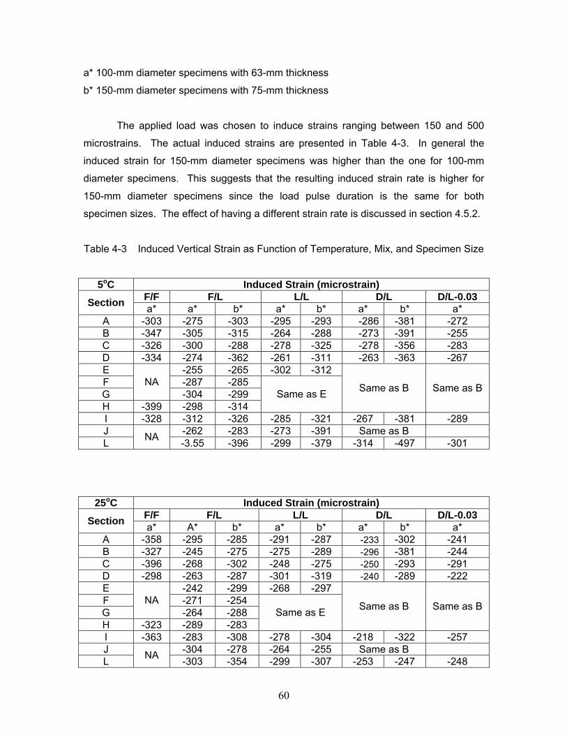
60

a* 100-mm diameter specimens with 63-mm thickness

b* 150-mm diameter specimens with 75-mm thickness

The applied load was chosen to induce strains ranging between 150 and 500

microstrains. The actual induced strains are presented in Table 4-3. In general the

induced strain for 150-mm diameter specimens was higher than the one for 100-mm

diameter specimens. This suggests that the resulting induced strain rate is higher for

150-mm diameter specimens since the load pulse duration is the same for both

specimen sizes. The effect of having a different strain rate is discussed in section 4.5.2.

Table 4-3 Induced Vertical Strain as Function of Temperature, Mix, and Specimen Size

5oC Induced Strain (microstrain) F/F F/L L/L D/L D/L-0.03 Section a* a* b* a* b* a* b* a*

A -303 -275 -303 -295 -293 -286 -381 -272 B -347 -305 -315 -264 -288 -273 -391 -255 C -326 -300 -288 -278 -325 -278 -356 -283 D -334 -274 -362 -261 -311 -263 -363 -267 E -255 -265 -302 -312 F -287 -285 G

NA -304 -299

H -399 -298 -314 Same as E Same as B Same as B

I -328 -312 -326 -285 -321 -267 -381 -289 J -262 -283 -273 -391 Same as B L NA -3.55 -396 -299 -379 -314 -497 -301

25oC Induced Strain (microstrain) F/F F/L L/L D/L D/L-0.03 Section a* A* b* a* b* a* b* a*

A -358 -295 -285 -291 -287 -233 -302 -241 B -327 -245 -275 -275 -289 -296 -381 -244 C -396 -268 -302 -248 -275 -250 -293 -291 D -298 -263 -287 -301 -319 -240 -289 -222 E -242 -299 -268 -297 F -271 -254 G

NA -264 -288

H -323 -289 -283 Same as E Same as B Same as B

I -363 -283 -308 -278 -304 -218 -322 -257 J -304 -278 -264 -255 Same as B L NA -303 -354 -299 -307 -253 -247 -248

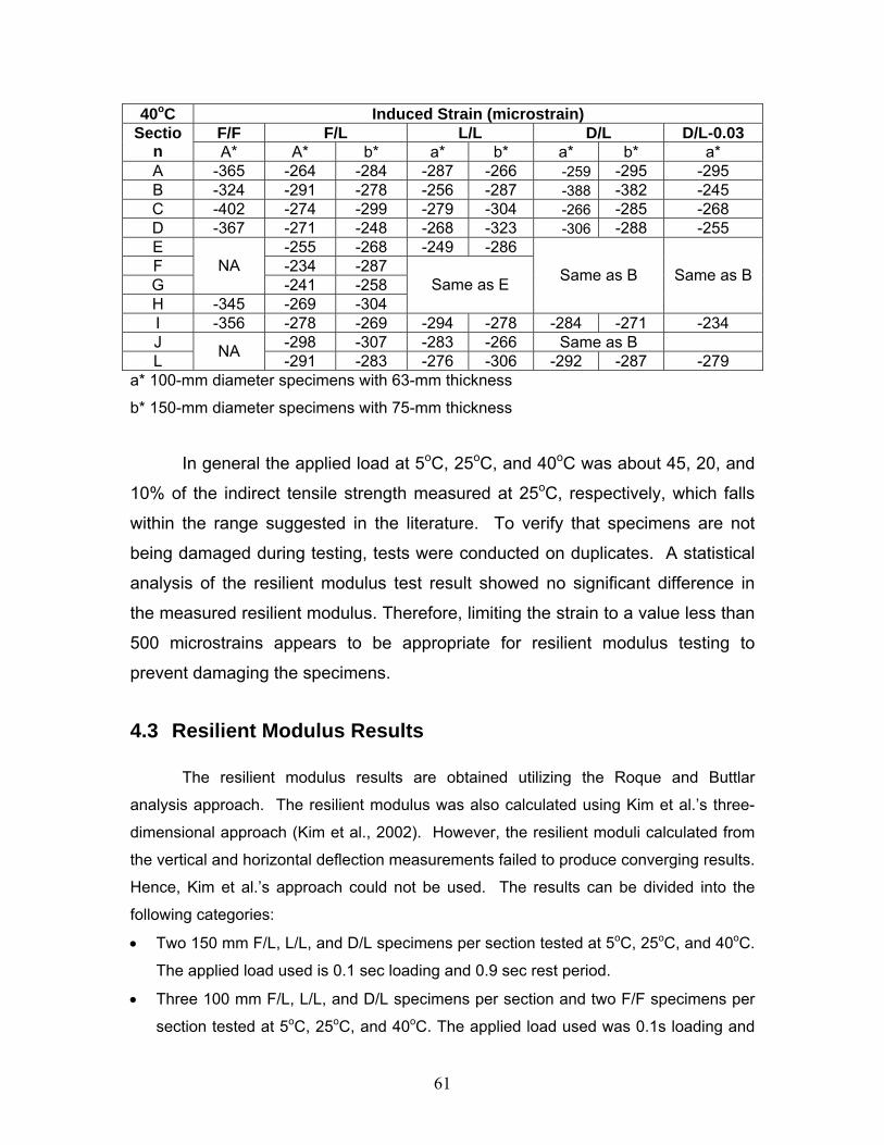
61

40oC Induced Strain (microstrain) F/F F/L L/L D/L D/L-0.03 Sectio

n A* A* b* a* b* a* b* a* A -365 -264 -284 -287 -266 -259 -295 -295 B -324 -291 -278 -256 -287 -388 -382 -245 C -402 -274 -299 -279 -304 -266 -285 -268 D -367 -271 -248 -268 -323 -306 -288 -255 E -255 -268 -249 -286 F -234 -287 G

NA -241 -258

H -345 -269 -304 Same as E Same as B Same as B

I -356 -278 -269 -294 -278 -284 -271 -234 J -298 -307 -283 -266 Same as B L NA -291 -283 -276 -306 -292 -287 -279

a* 100-mm diameter specimens with 63-mm thickness

b* 150-mm diameter specimens with 75-mm thickness

In general the applied load at 5oC, 25oC, and 40oC was about 45, 20, and

10% of the indirect tensile strength measured at 25oC, respectively, which falls

within the range suggested in the literature. To verify that specimens are not

being damaged during testing, tests were conducted on duplicates. A statistical

analysis of the resilient modulus test result showed no significant difference in

the measured resilient modulus. Therefore, limiting the strain to a value less than

500 microstrains appears to be appropriate for resilient modulus testing to

prevent damaging the specimens.

4.3 Resilient Modulus Results

The resilient modulus results are obtained utilizing the Roque and Buttlar

analysis approach. The resilient modulus was also calculated using Kim et al.’s three-

dimensional approach (Kim et al., 2002). However, the resilient moduli calculated from

the vertical and horizontal deflection measurements failed to produce converging results.

Hence, Kim et al.’s approach could not be used. The results can be divided into the

following categories:

• Two 150 mm F/L, L/L, and D/L specimens per section tested at 5oC, 25oC, and 40oC.

The applied load used is 0.1 sec loading and 0.9 sec rest period.

• Three 100 mm F/L, L/L, and D/L specimens per section and two F/F specimens per

section tested at 5oC, 25oC, and 40oC. The applied load used was 0.1s loading and

62

0.9 sec rest period. Three 100 mm D/L specimens per section tested at 5oC, 25oC,

and 40oC with an applied load of 0.03 sec loading and 0.97 sec rest period.

The results for the 100-mm specimens are presented in Table 4-4. In reviewing the

results, section I (SM-9.5A*) resulted in the highest resilient modulus. This result is

consistent for all test temperatures (5oC, 25oC, and 40oC), and is in accordance with

expectations since section I has a high compaction effort. On the other hand, SMA-12.5

(stone mastic asphalt mix) had, by far, the lowest resilient modulus at all three test

temperatures. SMA-12.5 has a fiber additive and higher asphalt content and percent

fines that may help in resisting fatigue and low temperature cracking.

With regard to the maximum nominal aggregate size of mixes SM-12.5D and

SM-9.5D, it was found that SM-12.5D was finer than what would be expected.

Therefore, the effect of aggregate size on resilient modulus could not adequately

investigated. Results of a comparison between F/L, L/L, and D/L reveal that although

the resilient modulus varies between the different sections, this variation is random and

no clear shift factor can be identified (within a mix, as well as for the same section

between the different mixes). It is clear, however, that there is a difference in resilient

modulus between the different mixes. The difference in measured resilient modulus

among F/L, L/L, and D/L specimens is believed to be due to the difference in volumetric

properties; the effect of volumetric properties on the resilient modulus is investigated in

section 4.6.

Each mix’s susceptibility to temperature is reflected by the change in resilient

modulus as a function of temperature. No conclusion can be made as to which binder

performs better in terms of resistance to temperature changes. However, due to its

relatively high asphalt content, the SMA-12.5 mix of section L proved to be the most

susceptible to temperature changes. As a conclusion, for the binders used in this

research, the binder content is thought to have an effect on the resilient modulus.

The effect of binder type is observed at 40oC between the PG 76-22 and the PG

64-22 (sections C and D, respectively). At that temperature, the PG 76-22 had a higher

resilient modulus for all the mixes. Differences between the PG 70-22 and the other

binder grades are inconsistent. The results of tests performed at 25oC also show an

inconsistency as to which binder grade performs better. At 5oC, the measured resilient

modulus was practically the same for both binder grades. As a conclusion, the effect of

the high temperature grade of the binder was found to be important at high temperatures

(40oC).

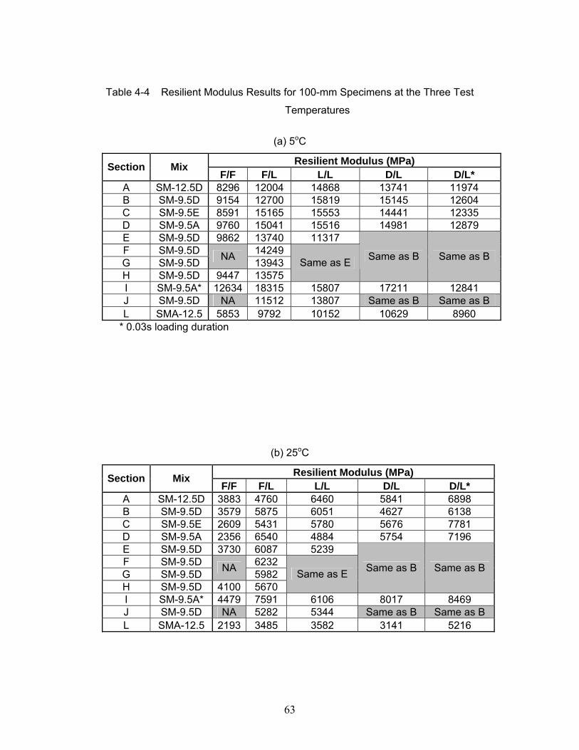
63

Table 4-4 Resilient Modulus Results for 100-mm Specimens at the Three Test

Temperatures

(a) 5oC

Resilient Modulus (MPa) Section Mix F/F F/L L/L D/L D/L*

A SM-12.5D 8296 12004 14868 13741 11974 B SM-9.5D 9154 12700 15819 15145 12604 C SM-9.5E 8591 15165 15553 14441 12335 D SM-9.5A 9760 15041 15516 14981 12879 E SM-9.5D 9862 13740 11317 F SM-9.5D 14249 G SM-9.5D NA 13943 H SM-9.5D 9447 13575

Same as E Same as B Same as B

I SM-9.5A* 12634 18315 15807 17211 12841 J SM-9.5D NA 11512 13807 Same as B Same as B L SMA-12.5 5853 9792 10152 10629 8960

* 0.03s loading duration

(b) 25oC

Resilient Modulus (MPa) Section Mix F/F F/L L/L D/L D/L*

A SM-12.5D 3883 4760 6460 5841 6898 B SM-9.5D 3579 5875 6051 4627 6138 C SM-9.5E 2609 5431 5780 5676 7781 D SM-9.5A 2356 6540 4884 5754 7196 E SM-9.5D 3730 6087 5239 F SM-9.5D 6232 G SM-9.5D NA 5982 H SM-9.5D 4100 5670

Same as E Same as B Same as B

I SM-9.5A* 4479 7591 6106 8017 8469 J SM-9.5D NA 5282 5344 Same as B Same as B L SMA-12.5 2193 3485 3582 3141 5216

64

(c) 40oC

Resilient Modulus (MPa) Section Mix F/F F/L L/L D/L D/L*

A SM-12.5D 1745 1926 2924 2703 3331 B SM-9.5D 1834 2517 2450 2116 3220 C SM-9.5E 1207 3347 2360 2691 3730 D SM-9.5A 968 2630 1966 2314 3023 E SM-9.5D 1843 1978 F SM-9.5D 2308 G SM-9.5D

NA 2325

H SM-9.5D 1899 2427 Same as E Same as B Same as B

I SM-9.5A* 1954 3320 2567 3484 5015 J SM-9.5D 2512 2112 Same as B Same as B L SMA-12.5

NA 1390 1224 1508 2301

*0.03s load duration

The resilient modulus results showed that mix characteristics and preparation,

and compaction method (laboratory gyratory compaction vs. field compaction) influence

resilient modulus values with the latter being more influential. As it can be seen from

Table 4-5, the measured resilient modulus fell in the same range for F/L, L/L, and D/L

specimens. However, the resilient modulus of field cores was distinctively lower than

that of either F/L, L/L, or D/L. Field/Lab and F/F specimens are obtained from the same

mix. The difference is in the way the specimens were compacted. On the other hand,

F/L, L/L, and D/L have the same compaction method but different mix characteristics.

Apart from sections I and L whose resilient moduli were significantly different, the

average resilient modulus at 5, 25, and 40oC are presented in Table 4-5.

Table 4-5. Average Resilient Modulus

F/F F/L L/L D/L

Temperature(oC) Mr

(MPa)

Variation

(%)

Mr

(MPa)

Variation

(%)

Mr

(MPa)

Variation

(%)

Mr

(MPa)

Variation

(%)

5 9185 6.9 13548 9.3 14480 11.6 14577 4.3

25 3676 21.3 5762 9.4 5626 10.3 5475 10.4

40 1531 27.2 2426 18.0 2298 15.9 2456 11.8

The difference in resilient modulus between F/F specimens and the other

specimen types, mainly F/L specimens, is substantial; therefore, a compaction shift

65

factor is necessary, if resilient modulus values of field cores and laboratory prepared

specimens are to be compared. The average resilient modulus for F/L, L/L, and D/L at

the three test temperatures is practically the same considering the calculated coefficient

of variation (Table 4-5). These three mixes where all compacted in the laboratory. As it

will be presented in section 4.6, the difference between the resilient modulus of the

different mixes measured for the same section, will be a result of the difference in

volumetric properties.

The load duration had also an effect on the resilient modulus. Results of D/L

specimens tested at 0.03 sec load duration are presented in Table 4-4. Excluding

sections I and L, the average resilient modulus was 12448, 7003, and 3326 MPa with a

coefficient of variation of 3.1, 9.8, and 9.0% at 5, 25, and 40oC, respectively, which is

considerably different from the results of D/L specimens tested at 0.1 sec load duration.

The different resilient modulus results at the two loading durations are analyzed in

section 4.5 which consists of the integration of a shift factor that relates 0.1 to 0.03 sec

loading duration test results.

The results presented in Table 4-4 are the average of three specimens (two

specimens for F/F). Two readings are taken from each specimen making a total of six

resilient modulus readings per section per mix (four for F/F specimens). The variability

in the readings is a measure of the IDT test repeatability; it can also be used as a

measure of homogeneity between the specimens of the same mix. Therefore, the

variability in the test results is presented in the following section.

4.4 Variability

The resilient modulus results reported in Section 4.3 represent the average of

measured test values. For mixes F/L, L/L, and D/L, the number of specimens used per

section for testing was three and two for 100- and 150-mm specimens, respectively.

Due to the fact that fewer specimens were available from the Virginia Smart Road, for

F/F mixes, only two 100 mm specimens were tested per available section. During

testing, readings are taken from the two faces of each specimen; therefore, two resilient

modulus values are obtained per specimen. Variation between the two reported values

per specimen can be traced to the inherent non-homogeneity of HMA, as well as

miscentering of the specimen. Non-homogeneity in HMA also occurs between different

specimens and can thus lead to differences in resilient modulus values between the

66

different specimens. Therefore, variations in resilient modulus can be classified into two

categories: within specimen variation and within mix variation. A discussion of each type

follows.

4.4.1 Within Specimen Variation

Variability of the calculated resilient modulus within the same specimen is due to

specimen miscentering and to the non-homogeneity of HMA. Since specimen

miscentering causes an imbalance in the net applied load between the two faces,

stresses within the specimen will, therefore, vary between the front and the back,

causing resilient modulus values to be overestimated on one side and underestimated

on the other. However, since resilient modulus values are independent of the applied

load (within the range of testing), the correct resilient modulus can be calculated by

averaging the resilient moduli calculated from each side of the specimen. The effect of

specimen miscentering on the stress distribution is presented in Figure 4-1. Variation

between the two sides is not due solely to specimen miscentering, but also to inherent

inhomogeneity of the mix. However, non-homogeneity can be estimated from the

variation between the specimens of the same mix, which is identified as the within mix

variability.

Figure 4-1 Stress Distribution

PPSpecimen offset

Actual stress distribution

Assumed stress distribution

P = Actual applied load P = Applied load with no offset

67

4.4.2 Within Mix Variation

Within mix variation represents the variation that occurs in the resilient modulus

due to inhomogeneity in the mix, which leads to different values of resilient modulus for

the different specimens tested. The within mix variation measures the repeatability of

the test setup used. In general, within mix variation that is smaller than the within

specimen variation indicates a good potential for repeatability. The variability in resilient

modulus calculation is summarized inTable 4-6.

Table 4-6 Resilient Modulus Variability

The maximum within specimen variability was 103.3%, 73.6%, 79.5%, 48.2%,

and 60.8% for F/F, F/L, L/L, D/L, and D/L-0.03 mixes, respectively; while the maximum

mix variability was 20.0%, 52.7%, 42.6%, 27.3%, and 21.9%, respectively. An

interesting observation was that results from the F/F specimen exhibited the highest

within specimen maximum variability of 103.3%, while at the same time possessing the

lowest maximum mix variability (20.0%). Moreover, it was observed from data analysis

Variability (in %) Temperature (oC) Mix

Type

5 25 40 Average/specimen 21.8 35.5 26.7

Average/mix 10.3 8.9 4.3 Maximum/specimen 103.3 F/F

Maximum/mix 20.0 Average/specimen 7.4 6.7 14.4

Average/mix 7.8 6.6 13.7 Maximum/specimen 73.6 F/L

Maximum/mix 52.7 Average/specimen 11.6 17.7 18.9

Average/mix 6.25 10.5 11.36 Maximum/specimen 79.5 L/L

Maximum/mix 42.6 Average/specimen 13.5 15.7 17.9

Average/mix 5.7 9.7 9.8 Maximum/specimen 48.2 D/L

Maximum/mix 27.3 Average/specimen 16.3 16.0 13.3

Average/mix 8.7 12.9 13.9 Maximum/specimen 60.8 D/L-0.03

Maximum/mix 21.9

68

that, in general, within specimen variability for F/F specimens was relatively high

compared to that of F/L, L/L, and D/L specimens, while the mix variability was roughly

equal, if not better. This suggests that homogeneity is more successfully achieved for

specimens compacted in the laboratory than for field cores, which can vary depending

upon the compaction quality. In addition, field core specimens were thinner than the

other specimens and therefore, any specimen offset will have a larger effect on the

specimen stress distribution.

The average specimen variability ranged between 6.7% and 35.5%, while the

average mix variability ranged between 5.7% and 13.9%. The average mix variability

results indicate that the repeatability of the indirect tension test for resilient modulus

calculation is good. As mentioned previously, variability within a specimen occurs as a

result of inhomogeneity and specimen miscentering. Since the minimum average mix

variability is 5.7% and the maximum average mix variability is 13.9%, while the

maximum average within specimen variability is 35.5%, an estimate of the maximum

average variability due to specimen miscentering would be between 21% and 30%.

4.5 Shift Factors

The main objective of this research was to account for the difference between the

resilient moduli of field cores (F/F specimens) and laboratory prepared specimens. For

this purpose, three different laboratory compacted mixes were prepared: F/L, L/L, and

D/L. Field cores were obtained from the Virginia Smart Road. The resilient modulus

results for F/L and F/F mixes showed that there is a discernible difference between the

designed and in-situ HMA layer properties. Lab/Lab specimens were prepared to

replicate F/L specimens; however, resilient modulus results and volumetric properties

revealed a difference between mixes prepared in the laboratory and the ones prepared

in the mixing plant. Differences between F/L, L/L, and D/L can be attributed solely to the

volumetric properties and are discussed in Section 4.6.

As a result of FWD testing and data of actual truck induced stresses and strains

measured at the Virginia Smart Road, loading pulse duration was another parameter

that was evaluated in this research. Hot-mix asphalt being a viscoelastic material, its

properties are time-dependent. In other words, the resilient modulus is believed to be

affected by both the load duration and the rest period. Currently, ASTM D4123-82

recommends the use of a load pulse duration of 0.1 sec and a rest period of 0.9 sec.

69

Based on FWD testing and actual stress and strain measurements taken from the field

at the Virginia Smart Road, Loulizi et al. (2002) suggested that at 0.03s load pulse

duration is more representative of actual traffic loading. Therefore, another set of 100-

mm specimens were mixed and compacted to be tested a 0.03s load pulse duration.

The resilient modulus calculated at 0.03 sec load pulse duration was then compared to

the resilient modulus of specimens tested at 0.1 sec load pulse duration and shift factors

were developed to account for the effect of load pulse duration. Finally, it was observed

that at 5oC, the resilient modulus of 100- and 150-mm specimens is the same. However,

at higher temperatures the different specimen sizes gave different resilient modulus

results. The discrepancy between the two specimen sizes increased as the test

temperature was increased.

The statistical analysis showed that there is a significant difference, which is not

attributed to the variation in the resilient modulus test, between the resilient modulus of

F/L and F/F specimens. Therefore, incorporating compaction shift factor (laboratory vs.

field compaction) is essential if resilient modulus values of field cores and laboratory

prepared specimens are to be compared.

4.5.1 Compaction Shift Factor

Different compaction methods are used in the field than in the laboratory.

Gyratory compaction is used in the laboratory to replicate field compaction. However,

there still are some differences between the two compaction methods. Some of these

differences are confinement and direction of compaction. Confinement is higher in the

laboratory than in the field. Compaction is performed in all directions in the laboratory,

while it is applied in the direction of traffic in the field.

Figure 4.1 shows the ratio of the resilient modulus of the 100 mm F/L specimens to the

resilient modulus of the F/F specimens at the three test temperatures. Except for the

SM-12.5D mix (section A) at 40oC, the resilient modulus of F/L specimens was clearly

higher than that of F/F specimens. For Section D (SM-9.5A), the compaction shift factor

increases considerably from 5oC to 25oC and then appears to level out at 40oC. Section

C (SM-9.5E) results also show an increasing shift factor with temperature. In general,

taking into account the variability in the IDT test, the shift factor appears to remain

constant at the three test temperatures. The increase with temperature in the

compaction shift factor for sections C and D can be explained by the fact that a higher

grade binder is used (section C has PG 76-22 asphalt grade and section D has PG 70-

70

22 asphalt grade). Indeed, the resilient modulus of both sections dropped dramatically

from 5oC to 25oC for the F/F specimens compared to the other sections: 8591 MPa to

2609 MPa for Section C and 11762 MPa to 2356 MPa for Section D. As for the

remaining mixes, the compaction shift factor varies between 1.23 and 1.70, with an

average of 1.46. A compaction shift factor between 1.45 and 1.50 seems to be

applicable to all the mixes, except sections C and D. The average shift factors are 1.45

at 5oC and 1.51 at 25oC (excluding sections C and D) and 1.45 at 40oC (excluding

sections A, C, and D). Data for section L (SMA-12.5) is not presented in Figure 4.1

since section L could not be tested at 40oC. However, tests performed at 5 and 25oC

resulted in a compaction shift factor of 1.63 and 1.59, respectively, which is slightly

higher than the average shift factor of the other sections. Section L has fiber which may

affect the shift factor.

0.50

1.00

1.50

2.00

2.50

3.00

3.50

0 10 20 30 40

Temperature (°C)

Shi

ft Fa

ctor

SM-12.5DSM-9.5DSM-9.5ESM-9.5ASM-9.5DSM-9.5A*

Figure 4-2 Compaction shift factor

Differences in the calculated resilient modulus between F/L and F/F specimens

can be attributed to compaction and, therefore, the bulk density and percent of air voids

content. The bulk density and percent of air voids content of the different F/L and F/F

mixes are summarized in Table 4-7.

71

Table 4-7 Percent Air Voids and Bulk Specific Gravity of F/L and F/F Specimens

Bulk Specific Gravity Air Voids (%)

Mix Mix Section

F/L F/F Ratio

F/L F/F Ratio

A 2.345 2.282 1.028 3.2 5.8 0.552

B 2.362 2.239 1.055 3.6 8.6 0.419

C 2.399 2.309 1.039 2.3 6 0.383

D 2.408 2.393 1.006 1.3 1.9 0.684

E 2.4 2.317 1.036 1.4 4.8 0.292

F 2.412 2.317 1.041 3.6 4.8 0.750

G 2.410 2.317 1.040 3.6 4.8 0.750

H 2.403 2.317 1.037 4.1 4.8 0.854

I 2.429 2.440 0.995 1.5 1.1 1.364

J 2.328 2.252 1.034 7.5 10.6 0.708

L 2.359 2.226 1.060 1.8 7.3 0.247

In general, the measured bulk specific gravity for F/L specimens is higher than

that for F/F specimens, which means that a better compaction was achieved in the

laboratory and, therefore, a higher resilient modulus value was measured for F/L

specimens. The same conclusion can be drawn from air void measurements, in which

F/L specimens had a much lower air voids content than F/F ones. The effect of bulk

specific gravity and air voids on the resilient modulus is discussed in Section 4.6, where

a model for predicting resilient modulus from volumetric properties is developed using

F/L, L/L, and D/L 100-mm specimens’ data. The F/F data is not used in the model

development due to the different compaction method used for F/F specimens. However,

the model can be used to verify if the compaction method has an effect which can not be

explained by the difference in volumetric properties on the resilient modulus. This task is

achieved by calculating the resilient modulus using the developed model, and comparing

it to the measured one from testing.

72

4.5.2 Specimen Size Shift Factor:

The resilient modulus calculation (Roque and Buttlar, 1992) is based on

correction factors used to correct the calculated stress, obtained from Hondros’ plain

stress solutions (Hondros, 1959), and the measured strain. These correction factors are

function of the diameter-to-thickness ratio and should be applicable to any specimen

diameter or thickness. Therefore, theoretically, after applying the correction factors, the

resilient modulus determined from 150-mm specimens should be the same as the one

determined from 100-mm specimens, after applying the correction factors. Figure 4.3a

is a plot of the resilient modulus ratio of 100- to 150-mm F/L specimens excluding

section D. It is evident that 100-mm specimen result in a higher resilient modulus. This

ratio varies between 0.81 and 1.41 (Figure 4.3a). The average shift factors between

100- and 150-mm F/L specimens are 0.98, 1.00, and 1.13 at 5oC, 25oC, and 40oC,

respectively, with an overall average of 1.04.

0.80

0.90

1.00

1.10

1.20

1.30

1.40

1.50

0 5 10 15 20 25 30 35 40 45Temperature (°C)

Shift

Fac

tor

SM-12.5D SM-9.5D section BSM-9.5-E SM-9.5D section ESM-9.5D section F SM-9.5D section GSM-9.5D section H SM-9.5A*SM-9.5D section J SMA-12.5

(a)

73

0.65

0.85

1.05

1.25

1.45

1.65

1.85

0 10 20 30 40Temperature (°C)

Shi

ft Fa

ctor

SM-12.5D SM-9.5D section BSM-9.5E SM-9.5ASM-9.5D section E SM-9.5A*SM-9.5D section J SMA-12.5

(b)

1.00

1.10

1.20

1.30

1.40

1.50

1.60

1.70

0 10 20 30 40

Temperature (°C)

Shift

Fac

tor

SM-12.5D SM-9.5DSM-9.5E SM-9.5ASM-9.5A* SMA-12.5

(c)

Figure 4-3 Specimen size shift factor (a) F/L specimens, (b) L/L specimens, and (c)

D/L specimens

74

From F/L results, it seems that the calculated resilient modulus is the same for

100- and 150-mm diameter specimens at all tested temperatures. However, results from

L/L and D/L do not support this finding. The average shift factor for L/L specimens was

1.04, 1.22, and 1.18 at 5oC, 25oC, and 40oC, respectively, with an overall shift factor of

1.15 (Figure 4.3b); while the average shift factor for D/L specimens was 1.23, 1.29, and

1.42 at 5oC, 25oC, and 40oC, respectively, with an overall shift factor of 1.31 (Figure

4.3c). It appears that D/L specimens have greater specimen size shift factor than L/L

specimens. Sections B, E, and J in D/L have unexpectedly low shift factors. Sections E

and J were not produced in D/L since they were identical to sections B. Therefore,

excluding these three sections, the specimen size shift factor for L/L specimens

becomes 1.15, 1.38, and 1.39 at 5, 25, and 40oC, respectively, which is comparable to

the results from D/L specimens. One interesting observation is that, while the specimen

size shift factor varies considerably between the three mixes, one general trend can be

seen; which is the fact that the specimen size shift factor increases as the temperature

increases. At 5oC, the average specimen size shift factor for the three mixes is 1.08.

Since the average variability for the three mixes at 5oC is 7.58%, and since the HMA

volumetric properties are not affected by the specimen size, this shift factor is most likely

due to variation in the resilient modulus test. Therefore, it is suggested that at 5oC the

resilient modulus obtained from 100- and 150-mm diameter specimens is comparable.

However, at 25oC the average specimen size shift factor increases to 1.17, which is

beyond the resilient modulus variation (COV = 10.00%), at that temperature. The

specimen size shift factor increases even more to 1.24 when the test temperature is

increased to 40oC. The average variability in the resilient modulus is 12.99%, at that

temperature.

At 5oC, HMA behaves as an elastic material with minimal viscous behavior. The

correction factors developed by Roque and Buttlar were developed for an elastic

material. They depend on the thickness to diameter ratio, and, therefore, the resilient

modulus obtained from 100- and 150-mm specimens is practically the same. As

temperature increases, HMA exhibits more viscous behavior. Therefore, the bulging,

which depends on Poisson’s ratio for elastic materials, will also be affected by the

amount of viscous flow that is exhibited in the material. The tested 150-mm diameter

specimens are relatively thinner than the tested 100-mm diameter specimens; the 150-

mm diameter specimens have a thickness to diameter ratio around 0.50, while this ratio

75

is around 0.625 for 100-mm diameter specimens. Hence, the viscous flow could

increase as the specimen’s thickness to diameter ratio decreases. This limits the

application of the correction factor when the materials behave more viscousely.

Moreover, the 150-mm diameter specimens are more representative since they

are expected to be less affected by aggregate size than 100-mm diameter specimens.

However, the resilient modulus variability analysis showed no significant difference

between 100- and 150-mm specimens, in that 100-mm specimens are more affected by

aggregate size. Therefore, it is suggested that, for mixes with maximum aggregate sizes

of 12.5mm and less, the resilient modulus determined from 100-mm specimens is as

representative of the overall mix as the one determined from 150-mm specimens.

4.5.3 Loading Duration Shift Factor

The resilient modulus of HMA is measured in the laboratory using a haversine

stress pulse. This haversine pulse is thought to replicate what actually occurs in the

pavement: While a truck tire is at a considerable distance from a point in the pavement,

the stress at that point is zero; when the tire is exactly on the considered point, the

stress is maximum. The loading time (duration) of the applied pulse was found to

depend on the truck speed and the depth below the pavement surface (Huang, 1993).

Since vehicle speed varies significantly and the depth of the material may not be known

during design, it was recommended that a haversine load duration of 0.1 sec and a rest

period of 0.9 sec be used for the laboratory test (Huang, 1993).

Loulizi et al. (2002) measured the vertical compressive stress pulse induced by a

moving truck and by FWD loading at different locations beneath the pavement surface.

They found that a haversine or a normalized bell-shape equation well represent the

measured normalized vertical compressive stress pulse of a moving vehicle. Haversine

duration times varied from 0.02s for a vehicle speed of 70km/h at a depth of 40mm, to 1s

for a vehicle speed of 10km/h at a depth of 597mm. For the FWD loading, a haversine

with a duration of 0.03s was found to well-approximate the induced stress pulse at any

depth below the pavement surface. The researchers recommended reducing the

loading time of HMA dynamic tests to 0.03s to better match loading times obtained from

moving trucks at average speed and from FWD testing. In light of these findings, this

study was conducted to evaluate the effect of reducing the pulse duration from 0.1 sec to

0.03 sec on the laboratory measured resilient modulus.

76

Because HMA is a viscoelastic material, its stress-strain relationship is time-

dependent; that is, for a given stress the calculated strain depends on the duration of

time for which the load is sustained. In general, for a given load intensity, the longer the

load application duration, the higher the induced stain, which leads to a lower resilient

modulus value. Two sets of 100 mm D/L specimens were tested at the same load

intensity for two different load durations. The load durations used are 0.1 sec loading

with a 0.9 sec rest period and 0.03 sec loading with a 0.97 sec rest period. A load-

duration shift factor was calculated as the ratio of the resilient modulus of specimens

tested at 0.03 sec load duration to the resilient modulus of specimens tested at 0.1 sec.

A statistical analysis of the difference in mean measured resilient modulus between the

test performed at 0.1 sec loading and the one performed at 0.03 sec was performed.

Since the two tests are independent, the paired t-statistic was performed. The paired t-

statistic was used instead of a regular t-test because each measurement from the IDT

performed at 0.1 sec loading can be matched to the measurement of the test performed

at 0.03 sec for the same mix. The parameter tested is the difference between the

means at α = 0.05. The results of the paired t-statistic are presented in Table 4-8. the

test shows that there is a significant difference between the resilient modulus measured

at 0.1 sec loading pulse and the resilient modulus measured at 0.03 sec loading pulse.

Figure 4-4 presents the shift factor of each section as a function of the test

temperature. As expected, the shift factor increases with the increase in test

temperature; this is due to the fact that viscoelastic properties of HMA become more

predominant as the mix temperature is increased. Theoretically, as the test temperature

is decreased, elastic behavior should become more dominant and, therefore, the

resilient moduli measured at the two different load durations should converge to the

same value.

Table 4-8. t-statistic at: (a) 5oC, (b), 25oC, and (c) 40oC.

(a)

0.1 sec load 0.03 sec load Mean 14358 11932 Hypothesized Mean Difference 0 df 5 P(T<=t) two-tail 0.001935352 t Critical two-tail 2.570577635

77

(b)

0.1 sec load 0.03 sec load Mean 5509.333333 6972.418456 Hypothesized Mean Difference 0 Df 5 t Stat -5.447955832 P(T<=t) two-tail 0.002830647 t Critical two-tail 2.570577635

(c)

Variable 1 Variable 2 Mean 2469.333333 3409.373682 Hypothesized Mean Difference 0 df 5 t Stat -6.921965475 P(T<=t) two-tail 0.000965239 t Critical two-tail 2.570577635

0.60

0.80

1.00

1.20

1.40

1.60

1.80

0 10 20 30 40Temperature (°C)

Shi

ft Fa

ctor

SM-12.5DSM-9.5DSM-9.5ESM-9.5ASM-9.5A*SMA-12.5

Figure 4-4 Load Duration Shift Factor

78

However, results of tests performed at 5oC produced a shift factor lower than 1

for all the tested sections, which would indicate that the measured strain induced by a

load sustained for a shorter period of time is higher than the one induced by the same

load sustained for a longer period of time, which is theoretically and practically

impossible. The explanation for a shift factor smaller than unity is related to the IDT test

execution. The resilient modulus test is a repetitive loading test. Hot-mix asphalt

experiences an accumulation of plastic strain during repetitive loading. However, the

accumulated plastic strain decreases with every new loading cycle and eventually

becomes negligible. The accumulated plastic strain per cycle is a function of the load

duration and increases with longer load durations. The resilient modulus test was run for

100 cycles for both loading durations, which may lead to a higher total accumulated

plastic strain for specimens tested for longer load durations. It is, therefore, possible that

the accumulated strain per cycle for specimens tested at shorter load durations will still

be significant and that those specimens need additional conditioning cycles, which will

lead to lower resilient moduli. The load duration shift factors varied between 0.75 and

0.87, 1.06 and 1.70, 1.23 and 1.53 with an average of 0.83, 1.31, and 1.39 at 5oC, 25oC,

and 40oC, respectively.

The development of shift factors (compaction, specimen size, and loading

duration shift factors) is possible when there is a significant difference in paired data;

meaning there is a significant difference in the data of the same section for different

mixes and the same pattern can be detected for all sections. These variations between

and within mixes are due to changes in volumetric properties and is discussed in the

following section.

4.6 Resilient Modulus Prediction from Volumetric and Binder Properties

The shift factor developed between the F/L and F/F specimens is due to the

differences in compaction that occur between the field and the laboratory. On the other

hand, F/L, L/L, and D/L specimens have all undergone the same laboratory compaction.

The calculated resilient modulus for those mixes will depend on other identified

parameters.

79

4.6.1 Factors Affecting Resilient Modulus

As expected, the resilient modulus was found to be highly dependent on the test

temperature. Correlation between the resilient modulus and the test temperature— with

the resilient modulus decreasing as temperature increases—is found to be highest and

best represented in an exponential form as follows (also see Figure 4-5): T

r eM βα −= (4.1)

where α and β are parameters that are functions of binder and mix properties

Using Equation 4.1, the fitted exponential relationship between the resilient

modulus and temperature incorporated two different coefficients, α and β, which varied

with the mix type (A through L) and preparation method (F/L, L/L, and D/L). The values

of α and β are presented in Table 4-9. The goodness of fit (R-square) for the different

sections is presented in Table 4-10. The different values of α and β suggest that,

although temperature is a major parameter affecting the HMA resilient modulus, other

parameters could also play a role affecting the resilient modulus of HMA. These

identified parameters can be mix properties, mainly bulk density, air voids, asphalt

binder content, voids in mineral aggregates, voids filled with asphalt, G*/sinδ, and fine to

asphalt ratio.

y = 17621e-0.0464x

R2 = 0.967

0

4000

8000

12000

16000

20000

0 10 20 30 40 50

Temperature (°C)

Res

ilien

t Mod

ulus

(MP

a)

Figure 4-5 Resilient Modulus Variation with Temperature (Specimen A1-4in D/L)

80

Table 4-9 Values of α and β

α (MPa) F/F F/L L/L D/L D/L-0.03 Sectio

n a* a* b* a* b* a* b* a*

A 11805 16168 12533 19103 12532 17621 10740 14978 B 11327 17348 10201 21020 15624 19533 10201 15603 C 11100 19146 11118 20649 11148 18222 11118 16212 D 13476 19720 16578 20200 11274 19846 11273 17118 E 19279 13089 15791 13575 F 19578 13200 G

NA 18751 14663

H 9119 17963 13499 Same as E Same as B Same as B

I 16146 23068 16872 20523 13441 21751 12653 15443 J 14561 12884 17522 12169 Same as B Same as B L NA 13105 10556 13841 7834 13676 6810 11511

a* 100-mm diameter specimens with 63-mm thickness

b* 150-mm diameter specimens with 75-mm thickness β (oC-1)

F/F F/L L/L D/L D/L-0.03 Section a* a* b* a* b* a* b* a*

A 0.0458 0.052 0.0629 0.046 0.0472 0.0464 0.0541 0.035 B 0.046 0.0471 0.0593 0.0527 0.0517 0.0568 0.0593 0.0401 C 0.0566 0.0492 0.0541 0.0538 0.0561 0.0478 0.0541 0.0348 D 0.0675 0.0472 0.0669 0.0564 0.0637 0.0533 0.0545 0.04 E 0.0538 0.0534 0.051 0.055 F 0.0512 0.0535 G

NA 0.0501 0.0535

H 0.0475 0.0489 0.059 Same as E Same as B Same as B

I 0.0486 0.0494 0.0544 0.0492 0.0551 0.0477 0.0538 0.0272 J 0.0431 0.05 0.0481 0.0498 Same as B Same as B L NA 0.0563 0.0598 0.0592 0.0708 0.057 0.0537 0.0365

81

Table 4-10 R2 Values for the Different Mixes

R2 F/F F/L L/L D/L D/L-0.03 Sectio

n a* a* b* a* b* a* b* a* A 0.81 0.99 0.85 0.98 0.96 0.97 0.98 0.83 B 0.95 0.96 0.98 0.95 0.91 0.95 0.98 0.89 C 0.95 0.93 0.95 0.94 0.94 0.96 0.95 0.82 D 0.99 0.95 0.92 0.94 0.99 0.93 0.97 0.86 E 0.93 0.98 0.92 0.91 F 0.92 0.98 G

NA 0.97 0.97

H 0.43 0.94 0.97 Same as E Same as B Same as B

I 0.98 0.92 0.95 0.94 0.92 0.91 0.92 0.79 J 0.98 0.97 0.86 0.98 Same as B Same as B L NA 0.96 0.98 0.96 0.97 0.94 0.95 0.77

The effect of each mix property on the calculated resilient modulus was

investigated. The procedure for determining the influence and importance of each

parameter includes identifying a trend in resilient modulus variation as a function of the

parameter being considered, analyzing the correlation between the resilient modulus

and each individual parameter, as well as the correlations between the considered

parameters. Five mix parameters were identified as affecting the parameters α and β

and therefore the resilient modulus. The parameters were considered in the

development of the model: bulk specific gravity (SG), air void (AV) content, asphalt

content (AC), voids in mineral aggregates (VMA), and fine to asphalt ratio (F/A), with

bulk specific gravity the most influential parameter on α and asphalt content the most

prominent for parameter β. The next step was to identify highly influential data points

and outliers. During the model building process, three data points were identified as

outliers; therefore, they were excluded from the model building process.

4.6.2 Model Development

The proposed model (Equation 4.1) includes two coefficients that depend on the

mix properties. Coefficient α represents the resilient modulus at 0°C, while coefficient β

represents the sensitivity of the resilient modulus to temperature changes. Using

Equation 4.1, the coefficients α and β were determined for each section. One dilemma

in developing a model arises from uncertainty about which terms to include in the model.

Since five parameters had to be investigated, all possible regressions (25=32) were

82

considered. The final model selected is based on a goodness of fit and a goodness of

prediction criteria.

To validate a certain model, data is usually split into two sets—one set for model

fitting and another set to validate the prediction capabilities of the developed model.

Data splitting requires extensive gathering of data. An alternative to this process

involves calculating the PRESS statistic, which is a measure of a model’s prediction

capabilities, which can be used as a form of validation in the spirit of data splitting. The

PRESS statistic is computed as the sum of squares of the PRESS residuals. The

procedure involves setting aside the first observation from the data set and using the

remaining n-1 observations to estimate the coefficients for a particular candidate model.

The first observation is then replaced and the second observation withheld with

coefficients estimated again. Each observation is removed one at a time, and thus the

candidate model is fitted n times. The deleted response is estimated each time,

resulting in n prediction errors. The model that is finally adopted is fit using the entire

data set, making use of all available information. The model with the lower PRESS

statistic is the one that performs the best for prediction.

Another prediction parameter, the Cp statistic, was also considered during model

selection. The Cp statistic is a compromise between model underfitting and model

overfitting. The model with the lower Cp presents the best compromise between

overfitting and underfitting. The models were also evaluated for fitting ability in the form

of RMSE and the R-squared. In terms of fitting, the model with the higher R-square and

lower MSE is the best model. It should be noted that different models might have

optimum PRESS statistic, Cp, R-square, or MSE. In the end, the best overall model, a

compromise between fitting and predicting capabilities, was selected.

The data used for model development was obtained from 100 mm F/L, L/L, and

D/L specimens. The values of α and β, as well as the R-square (obtained by fitting

equation 4.1 to the data of the measured resilient modulus) is presented in Table 4.6.

Alpha (α) was found to be related to the bulk density, the asphalt content, as well

as to the fine-to-asphalt ratio, while β was found to be related to the bulk density, the

natural log of asphalt content, and the voids in mineral aggregates. The relationships for

α and β are presented in equations 4.2 and 4.3, respectively.

α = 59283.91 SG – 1285.19 AC -2109.91 F/A -112749.23 (4.2)

β = 0.11276 - 0.040328 SG + 0.032212 ln(AC) -0.001417101 VMA (4.3)

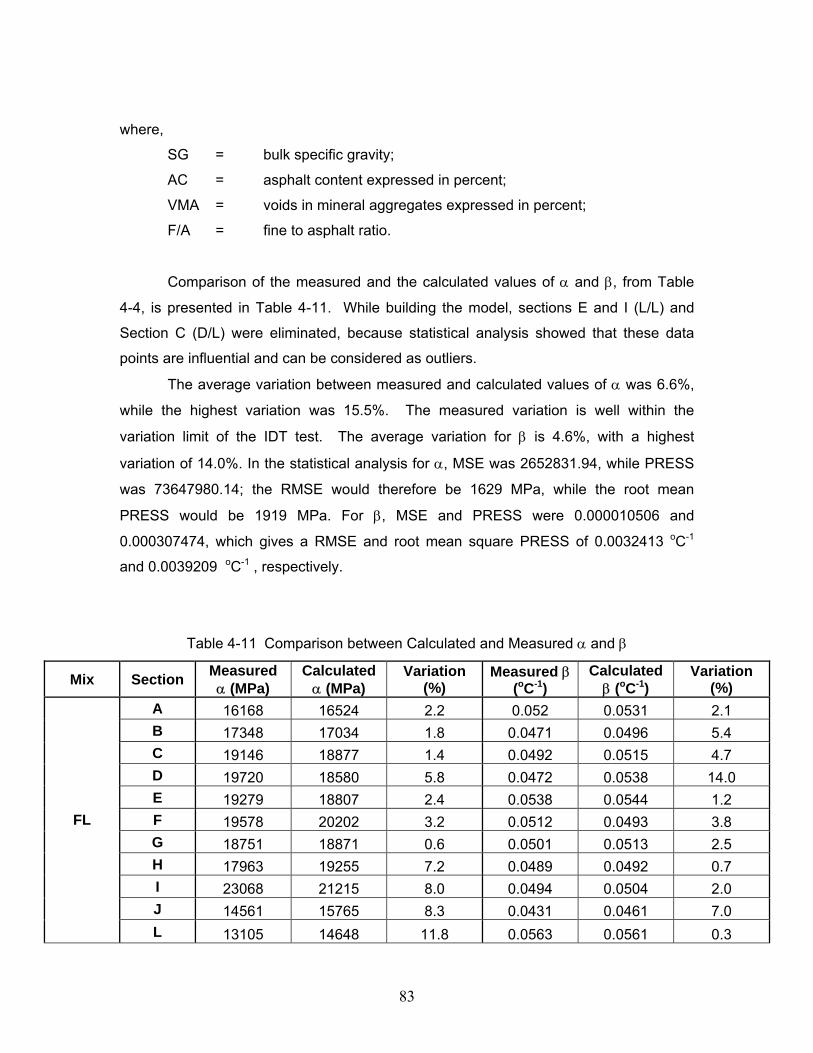
83

where,

SG = bulk specific gravity;

AC = asphalt content expressed in percent;

VMA = voids in mineral aggregates expressed in percent;

F/A = fine to asphalt ratio.

Comparison of the measured and the calculated values of α and β, from Table

4-4, is presented in Table 4-11. While building the model, sections E and I (L/L) and

Section C (D/L) were eliminated, because statistical analysis showed that these data

points are influential and can be considered as outliers.

The average variation between measured and calculated values of α was 6.6%,

while the highest variation was 15.5%. The measured variation is well within the

variation limit of the IDT test. The average variation for β is 4.6%, with a highest

variation of 14.0%. In the statistical analysis for α, MSE was 2652831.94, while PRESS

was 73647980.14; the RMSE would therefore be 1629 MPa, while the root mean

PRESS would be 1919 MPa. For β, MSE and PRESS were 0.000010506 and

0.000307474, which gives a RMSE and root mean square PRESS of 0.0032413 oC-1

and 0.0039209 oC-1 , respectively.

Table 4-11 Comparison between Calculated and Measured α and β

Mix Section Measured α (MPa)

Calculated α (MPa)

Variation (%)

Measured β (oC-1)

Calculated β (oC-1)

Variation (%)

A 16168 16524 2.2 0.052 0.0531 2.1 B 17348 17034 1.8 0.0471 0.0496 5.4 C 19146 18877 1.4 0.0492 0.0515 4.7 D 19720 18580 5.8 0.0472 0.0538 14.0 E 19279 18807 2.4 0.0538 0.0544 1.2 F 19578 20202 3.2 0.0512 0.0493 3.8 G 18751 18871 0.6 0.0501 0.0513 2.5 H 17963 19255 7.2 0.0489 0.0492 0.7 I 23068 21215 8.0 0.0494 0.0504 2.0 J 14561 15765 8.3 0.0431 0.0461 7.0

FL

L 13105 14648 11.8 0.0563 0.0561 0.3

84

Mix Section Measured α (MPa)

Calculated α (MPa)

Variation (%)

Measured β (oC-1)

Calculated β (oC-1)

Variation (%)

A 19103 16135 15.5 0.046 0.0483 5.0 B 21020 22643 7.7 0.0527 0.0493 6.5 C 20649 20527 0.6 0.0538 0.0510 5.3 D 20200 20897 3.4 0.0564 0.0540 4.3 E 15791 20920 32.5 0.051 0.0516 1.1 I 20523 16258 20.8 0.0492 0.0474 3.6 J 17522 20227 15.4 0.0481 0.0470 2.2

LL

L 13841 14773 6.7 0.0592 0.0553 6.6 A 17621 18497 5.0 0.0464 0.0486 4.8 B 19533 18402 5.8 0.0568 0.0489 13.8 C 18222 20987 15.2 0.0478 0.0524 9.6 D 19846 17915 9.7 0.0533 0.0520 2.4 I 21751 18723 13.9 0.0477 0.0484 1.6

DL

L 13676 14838 8.5 0.057 0.0544 4.6 Average 6.6 4.6

4.6.3 Model Evaluation

Finally, the capability of the proposed model to estimate HMA resilient modulus

was evaluated. Using Equation 4.4, the average measured resilient modulus of each

section was compared to the calculated one at the three test temperatures. The results

are presented in Table 4-12, while Error! Reference source not found. presents the

calculated resilient modulus vs. the measured resilient modulus, as well as any deviation

from the equality line. The difference between the measured and predicted resilient

moduli varied between 0.1 and 42.8%, with an average of 12.3% and a standard

deviation of 9.3%. The greatest difference between measured and calculated resilient

moduli is shown in section E L/L. This result was expected since data from section E of

L/L was considered an outlier due to the high bulk density. The average variation

between the calculated and measured resilient moduli was 7.9%, 11.0%, and 13.2%,

while the standard deviation was 8.2%, 8.5%, and 10.6% at 5oC, 25oC, and 40oC,

respectively. Considering that the average mix variability ranges between 5.7% and

13.9%, the variation between the measured and calculated resilient moduli is very good.

Therefore, the developed model can be considered to predict accurately the resilient

modulus of HMA measured by the indirect tension test setup.

85

Table 4-12 Comparison between Calculated and Measured Resilient Modulus

5°C 25°C 40°C

Measured Mr (MPa)

Calculated Mr (MPa) Variation Measured

Mr (MPa) Calculated Mr (MPa) Variation Measured

Mr (MPa) Calculated Mr (MPa) Variation

12004 12760 5.5% 4760 4411 8.0% 1926 1988 2.5% 13276 13088 0.1% 5782 4850 14.8% 2517 2303 7.1% 15165 14911 3.8% 5431 5321 4.1% 2837 2457 15.3% 15041 13764 5.6% 6540 4691 26.0% 2895 2092 25.5% 13740 13963 4.3% 6087 4700 20.8% 2083 2077 2.3% 14249 15791 10.8% 6232 5896 5.4% 2308 2816 22.0% 13943 14083 4.7% 5982 5044 12.6% 2325 2336 4.1% 13575 15164 10.9% 6133 5664 8.3% 2427 2706 10.7% 18315 17344 10.0% 6843 6327 12.1% 3320 2970 15.0% 11512 12467 8.7% 5282 4956 5.8% 2512 2482 0.8%

F/L

9792 10919 13.0% 3485 3553 3.3% 1390 1531 11.6% 14868 13770 14.8% 6460 5241 25.3% 2924 2539 20.1% 15819 17960 11.9% 6051 6704 9.2% 2450 3201 28.8% 15553 15884 2.3% 5780 5732 0.7% 2360 2669 13.3% 15060 15716 6.0% 5353 5341 1.3% 1966 2378 22.8% 11317 16251 42.8% 5239 5791 9.9% 1877 2671 41.5% 15807 14202 18.8% 6405 5503 22.4% 2823 2702 13.5% 13807 14041 15.8% 5344 5480 16.7% 2723 2706 13.1%

L/L

10152 11177 10.4% 3418 3697 8.4% 1224 1613 32.1% 13741 15553 5.6% 5841 5881 6.1% 2703 2836 2.2% 15145 13845 4.9% 4627 5203 17.0% 2116 2497 22.8% 14441 16480 11.8% 5676 5781 0.2% 2691 2635 4.0% 14981 14336 7.8% 5754 5066 15.2% 2314 2321 3.3% 17211 15692 14.6% 8017 5955 30.4% 3484 2879 22.6%

D/L

10629 10608 6.4% 3141 3575 21.3% 1508 1581 11.7% Average 8.0% 11.03% 13.23%

86

0

2000

4000

6000

8000

10000

12000

14000

16000

18000

20000

0 5000 10000 15000 20000Measured Mr (MPa)

Cal

cula

ted

Mr (

MP

a)

Figure 4-6 Calculated vs. Measured Mr

4.6.4 Resilient Modulus Calculation for F/F Specimens

In Section 4.5.1, it was observed that the resilient modulus of F/F specimens

varied from that of F/L specimens. Likewise, the bulk density and percent of air voids in

both set of specimens differed. Since the resilient modulus is related to the bulk density,

the difference between the resilient moduli of F/F and F/L specimens could be solely due

to the differences in bulk density. Therefore, the resilient modulus of F/F specimens was

calculated, using the previously developed model, and then compared to the measured

one. The results are presented in Table 4-13. The difference between the calculated

and measured resilient moduli varies between 1.3% (Section A at 5oC) and 107%

section D (40oC). The average variation was 29.3%, with a standard deviation of

26.13%.

87

Table 4-13 Comparison between calculated and measured F/F resilient modulus

Temperature (oC) Section Measured Mr (MPA) Calculated Mr (MPa) Difference (%)

A 9559 9682 1.29

B 9154 7414 19.01

C 8591 10278 19.64

D 11762 13476 14.57

E 9862 10401 5.47

F

G NA NA NA

H 9447 10877 15.14

I 13507 17032 26.10

J NA NA NA

5

L 5853 4973 15.04

A 3883 3181 18.08

B 3579 2488 30.49

C 2609 3411 30.74

D 2356 4537 92.59

E 3730 3274 12.21

F

G NA NA NA

H 4100 3791 7.55

I 4479 6269 39.96

J NA NA NA

25

L 2193 1454 33.72

A 2030 1380 32.01

B 1834 1097 40.20

C 1207 1491 23.56

D 968 2006 107.19

E

F

G

NA NA NA

H 1899 1719 9.46

I 1954 2962 51.60

J

40

L NA NA NA

88

However, such a high average variation is partly due to the variations that occur

in section D at 25oC and 40oC. Quite unexpectedly, the resilient modulus measurements

for section D at 25oC and 40oC were very low, which is probably due to the specimens

being damaged; therefore, these measurements should be considered non-reliable and

should be excluded from the analysis. Doing so would give a maximum variation of

51.6% (section I at 40oC). The average variation would then be 22.3%, with a standard

deviation of 13.1%. The average variation between the model-calculated and measured

resilient moduli is higher than the average mix variability in the resilient modulus test:

10.3%, 8.9%, and 4.3% at 5oC, 25oC, and 40oC, respectively. However, test results of

F/F specimens are based on limited number of data as a result of the limited number of

field cores, as well as the inability to test some specimens at 25 and/or 40oC. In

conclusion, the difference in the measured resilient moduli between F/L and F/F

specimens is partly due to the difference in the volumetric properties, mainly the bulk

density. However, the difference in bulk density does not fully explain this difference,

which confirms the existence of a compaction shift factor between field cores and

laboratory prepared specimens.

4.7 Conclusion

Resilient modulus values were successfully measured using the IDT setup. The

mix variability was determined and it was found that the repeatability of the IDT test is

high. Shift factors for compaction, and load duration were developed. Field compaction

resulted in field cores having lower bulk density and higher air voids than F/L specimens,

however, this fact did not entirely explain the difference in the measured resilient

modulus. The data analysis method used to calculate the measured resilient modulus

(Roque and Buttlar, 1992) was developed to take into account the specimen size effect

by introducing correction factors that are function of the specimen diameter to thickness

ratio. The method is applicable at low temperature, however as the testing temperature

is increased elastic analysis lead to discrepancies between the 100- and 150-mm

specimen diameter resilient modulus values. The load duration was found to have an

effect on the measured resilient modulus. The effect of load duration increased with

increasing temperature. However an interesting finding was the fact that the resilient

modulus measured at 0.1 sec load duration was higher than the one measured at 0.03

sec load duration at 5oC, which might be related to the method the IDT test is performed.

89

Finally a model predicting resilient modulus values from volumetric properties was

successfully developed. The resilient modulus values predicted by the model fell well

within the range of the test variability.

90

Chapter 5 Findings, Conclusions, and Recommendations

5.1 Summary

Accurate determination of the material properties is essential for pavement design,

maintenance, and rehabilitation. Laboratory testing has the advantage of determining

the material properties before the pavement is constructed. Upon completion of the

construction, the as built material properties can be determined using FWD testing or by

laboratory testing of field cores. The main objective of this research was to develop shift

factors between field cores and laboratory prepared specimens. Determining these shift

factors allows pavement engineers to determine whether the difference between the

laboratory prepared specimens or field cores resilient modulus is due to compaction or

construction. Moreover, such a shift factor is important during the design stage when

resilient modulus values can be obtained from specimens prepared in the laboratory.

Laboratory specimens were prepared using HMA either mixed at the plant during

construction or mixed in the laboratory. Also the effect of load pulse duration on the

resilient modulus was investigated. The load pulses investigated are 0.1s (as

recommended by ASTM D4123) and 0.03s (based on a study on the stress pulse width

and truck loading by Loulizi et al., 2002). The tasks that were undertaken in this

research can be summarized as follows:

1. Specimen preparation; the specimens were divided into F/F, F/L, L/L, D/L, and

D/L tested at 0.03s load pulse duration.

2. Determine the load to be used for resilient modulus testing at each of the testing

temperatures for the different mixes. The selected load had to meet the criterion

of limiting the strain between 150 and 500 microstrains.

3. Determine the variability in the IDT test. The variability was divided into two

parts: (1) variability between the two faces of the IDT specimen, and (2)

variability between the specimens of a given mix.

4. Determine the compaction shift factor at each of the testing temperatures

between F/F, and F/L specimens.

5. Determine the specimen size shift factor between 100- and 150-mm diameter

specimens for F/L/, L/L, and D/L specimens.

91

6. Determine the load pulse duration shift factor between 0.1s and 0.03s load

pulses; this was performed on D/L specimens.

7. Develop a model to correlate the resilient modulus to the temperature and the

volumetric properties of the HMA using F/L, L/L, and D/L specimens. This model

was then used to calculate the resilient modulus of F/F specimens and compare

the results to the measured resilient modulus of F/F specimens.

5.2 Findings

Various findings were encountered during this research. These findings can be

summarized as follows:

1. In the tested load range, the resilient modulus was found to be independent of

the applied load at 5oC and 25oC. This could not be verified at 40oC due to the

limited range of tested loads. The reason for the independence of the resilient

modulus to the load intensity is thought to be due to the fact that the tested load

range is relatively small compared to the indirect tensile strength of the

specimens.

2. Damage to an indirect tension specimen is avoided when the strain is limited

between 150 and 500 microstrain.

3. The average specimen variability ranged between 6.7% and 35.5%, while the

average mix variability ranged between 5.7% and 13.9%. This indicates that the

repeatability of the indirect tension test for resilient modulus calculation is

acceptable. Moreover it was found that repeatability is better achieved for

specimens produced in the laboratory than for specimens taken from the field.

4. The study showed that there is a compaction shift factor between field cores and

laboratory compacted specimens. The shift factor ranged from 1 to 3 with

laboratory compacted samples having the higher resilient modulus. An average

shift factor ranging between 1.45 and 1.5 seems to represent most mixes at all

tested temperatures. The existence of a shift factor is reinforced by the fact that

different air void content and specific gravity were measured for F/F and F/L

samples.

5. The data analysis procedure used in calculating the resilient modulus accounted

for the specimen size effect at 5oC. At 5oC the behavior of HMA is elastic and

therefore correcting for the specimen size using an elastic analysis resulted in a

92

consistent resilient modulus measured for 100- and 150-mm diameter.

However, at 25 and 40oC, viscous flow in the specimen resulted in different

resilient modulus from 100- and 150-mm diameter specimens, with the former

resulting in a higher calculated resilient modulus. The specimen size shift factor

increased as the test temperature increased. The average specimen size shift

factor was 1.25, and 1.30 at 25, and 40oC, respectively.

6. Analysis of the variability in resilient modulus results showed no difference

between 100- and 150-mm diameter specimens which means that 100-mm

diameter specimens as accurate as 150-mm diameter specimens in determining

the resilient modulus however, the measured values are not the same.

7. The average load duration shift factor varied with temperature, with average load

duration shift factors of 0.83, 1.31 and 1.39 at 5oC, 25oC, and 40oC, respectively.

These shift factors represent the ratio of the measured resilient modulus at 0.03

sec to the measured resilient modulus at 0.1 sec load duration. An interesting

result is the load duration shift factor at 5oC which is smaller than one. The

explanation for this fact is that the total accumulated strain using a load duration

of 0.1 sec is higher than the one accumulated using a load duration of 0.03 sec.

This might lead to lower resilient moduli being measured at a 0.03 sec loading

duration. This factor was verified by measuring the resilient modulus at 0.03 sec

and 0.1 sec on the same samples which also produced the same shift factor.

8. In characterizing the resilient modulus as a function of temperature, two

parameters α and β were identified. α is related to the resilient modulus at 0oC

while β represents the mix sensitivity to temperature. These two parameters were

related to the mix volumetric properties. α was found to be affected by the mix

specific gravity, the asphalt content, and the fine to asphalt ratio; while β was

found to be affected by the asphalt content, the specific gravity, and the voids in

mineral aggregates. A model was developed to predict the resilient modulus from

the mix volumetric properties. The average variation between the model

calculated and measured resilient modulus was 7.95%, 11.03%, and 13.23% at

5oC, 25oC, and 40oC, respectively, which is lower than the average mix variation

in the indirect tension test for the resilient modulus.

93

5.3 Conclusions

The resilient moduli of the different HMA placed at the Virginia Smart Road were

measured in the laboratory using the IDT setup. The variability in the result was

determined and shift factors were developed to account for the effect of compaction,

specimen size, and load pulse duration. Finally, a model that relates the resilient

modulus to the volumetric properties of the mix was developed. Based on this research,

the following conclusions could be drawn:

1. The testing results suggest that as long as the applied load is under 20% of the

load to cause failure in the specimen, the resilient modulus of HMA will be

independent of the applied load; this is based on results of tests at 25oC.

2. There is a difference between field compaction and laboratory gyratory

compaction. The difference results in different resilient moduli between field

cores and laboratory produced specimens and cannot fully be explained by the

fact that the percent air voids and bulk specific gravity are different for the two

sets of specimens.

3. The load duration affects the resilient modulus results. Therefore, resilient

modulus results obtained at loading durations similar to the ones experienced in

the field should be used for HMA characterization.

4. There is a strong correlation between the resilient modulus of HMA and its

volumetric properties. These volumetric properties are the bulk specific gravity,

the asphalt content, the fine to asphalt ratio, and the voids in mineral aggregate.

A model was developed to predict the HMA resilient modulus from its volumetric

properties

5.4 Recommendations

Based on the research’s results the following recommendations for testing and future

research can be made:

1. It is clear that the load duration has an effect on the measured resilient modulus

therefore, it is suggested that a load pulse duration of 0.03 sec be used since it is

more representative of the actual traffic loading.

2. The range of the applied load in this research was small compared to the indirect

tensile strength of the HMA. In this range, the load had no effect on the

94

measured resilient modulus. To investigate the effect of load intensity on the

measured resilient modulus using Roque and Buttlar’s data analysis, the Load

intensity range must be increased. Roque and Buttlar showed that a strain of

2000 microstrain may be needed to induce damage to the samples; therefore,

the loading can be safely increased to investigate its effect on the resilient

modulus.

3. The shift factor between field and laboratory compaction might be partly due to

the difference in the sample thickness between F/F and F/L samples. To fully

account for the effect of compaction, specimens of the same thickness and same

diameter to thickness ratio should be tested.

4. it appears that the viscous flow of HMA in the resilient modulus testing is affected

by the thickness to diameter ratio. To quantify this effect, it is suggested that a

wider range of specimen diameters and thicknesses be investigated.

5. To quantify the effect of HMA volumetric properties on its resilient modulus for

different mixes, it is suggested that a wider range of volumetric and binder

properties be used to fine-tune and calibrate the developed model for other HMA.

95

References

Almudaiheem, J., and Al-Sugair, F., “Effect of Loading Magnitude on Measured Resilient Modulus of Asphalt Concrete Mixes.” Transportation Research Record, No.1317, Transportation Research Board, Washington, DC, pp.139-144, 1991. Baladi, Gilbert Y. Harichandran, Ronald S. Lyles, Richard W. “New relationships between structural properties and asphalt mix parameters.” Transportation Research Record n 1171 1988 p 168-177 Blakey, F.A., and Beresford, F.D., “Tensile Strain in Concrete” II. C.S.I.R.O. Div. Build. Res. Rep. No. C2. 2-2, 15, 1955. Brown, E.R., and Foo, Kee Y., “Evaluation of Variability in Resilient Modulus Test Results (ASTM D 4123)”, ASTM Journal of Testing & Evaluation, Vol. 19 No 1, p 1-13, 1991. Cragg R. Pell PS. “Dynamic stiffness of bituminous road materials” Proceding of the Association of Asphalt Paving Technologists, Tech Session, Oklahoma City, Okla,. v 40 Feb 15-17 1971 p 126-47 Gemayel, Chaouki A. Mamlouk, Michael S. Characterization of hot-mixed open-graded asphalt mixtures. Transportation Research Record n 1171 1988 p 184-192 Heinicke, John J. Vinson, Ted S. “EFFECT OF TEST CONDITION PARAMETERS ON IRMR”. Journal of Transportation Engineering. v 114 n 2 Mar 1988 p 153-172 Hondros, G., “The Evaluation of Poisson’s Ratio and the Modulus of Materials of a Low Tensile Resistance by the Brazilian (Indirect Tensile) Test with Particular Reference to Concrete”, Australian Journal of Applied Science, Vol. 10, No. 3, p. 243-268, 1959. Howeedy, M Fayek, Herrin, Moreland. BEHAVIOR OF COLD MIXES UNDER REPEATED COMPRESSIVE LOADS. Highw Res Rec. n 404, 1972 p 57-70 Kim, Y.R., Shah, K.A, and Khosla, N.P, “Influence of Test Parameters in SHRP P07 Procedure on Resilient Moduli of Asphalt Concrete Field Cores”, Transportation Research Record 1353, p.82-89, 1992. Lim, C.T., Tan, S.A., Fwa, T.F., “Specimen Size Effect on The Diametrical Mechanical Testing of Asphalt Mixes”, Journal of Testing and Evaluation, JTEVA, Vol. 23, No. 6, pp. 436-441, 1995.

96

Loulizi, A., Al-Qadi, I.L., Lahour, S., and Freeman, T.E., “Measurement of Vertical Compressive Stress Pulse in Flexible Pavements and Its Representation for Dynamic Loading”, Transportation Research Board, Paper No.02-2376, 2002. Myers, R.H., “Classical and Modern Regression with Applications”, second edition Roque, R., and Ruth, B.E., “Materials Characterization and Response of Flexible Pavements at Low Temperatures.” Proceedings of the Association of Asphalt Paving Technoligists, Vol. 56, pp. 130-167, 1987. Roque, R., and Buttlar, W.G., “Development of a Measurement and Analysis Method to accurately Determine Asphalt concrete Properties Using the Indirect Tensile Mode”, Proc., Association of Asphalt Paving Technologists, Vol. 61, 1992. Schmidt, R J. “PRACTICAL METHOD FOR MEASURING THE RESILIENT MODULUS OF ASPHALT-TREATED MIXES.” Highway Research Record n 404, 1972 p 22-29 15. Von Quintus, Harold L. Harrigan, Edward. Lytton, Robert L. How SHRP reliably predicts pavement performance Pacific Rim TransTech Conference. Publ by ASCE, New York, NY, USA. 1993. p 298-307 Wright, P.J.F., “Comments on an indirect tensile test for concrete” Mag. Conc. Res. 20: 87-96, 1955.

97

Appendix A

Mixture Designs and Gradations

98

%#78 Quartzite Salem Stone Co., Sylvatus, VA 15#8 Quartzite Salem Stone Co., Sylvatus, VA 30#9 Quartzite Salem Stone Co., Sylvatus, VA 10

#10 Limestone Sisson and Ryan Quarry, Shawsville, VA 20Sand Castle Sand Co., New Castle VA 10

Fine RAP Adams Construction Co., Blacksburg, VA 15%

PG 70-22 Associated Asphalt, Inc., Roanoke, VA 5.6

%#78 Quartzite Salem Stone Co., Sylvatus, VA 5#8 Quartzite Salem Stone Co., Sylvatus, VA 30#9 Quartzite Salem Stone Co., Sylvatus, VA 20

#10 Limestone Sisson and Ryan Quarry, Shawsville, VA 20Sand Castle Sand Co., New Castle VA 10

Fine RAP 15%

PG 70-22 Associated Asphalt, Inc., Roanoke, VA 5.9Binder

Binder

Design / LabAggregate

Lab / LabAggregate

Figure A.1 Mixture designs for SM12.5D, section A.

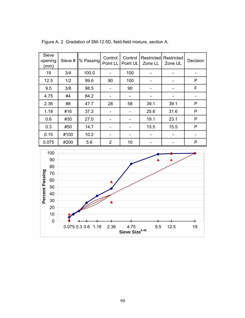
99

Figure A. 2 Gradation of SM-12.5D, field-field mixture, section A.

Sieve opening

(mm)Sieve # % Passing Control

Point LLControl

Point ULRestricted Zone LL

Restricted Zone UL Decision

19 3/4 100.0 - 100 - - -

12.5 1/2 99.6 90 100 - - P

9.5 3/8 98.5 - 90 - - F

4.75 #4 84.2 - - - - -

2.36 #8 47.7 28 58 39.1 39.1 P

1.18 #16 37.3 - - 25.6 31.6 P

0.6 #30 27.0 - - 19.1 23.1 P

0.3 #50 14.7 - - 15.5 15.5 P

0.15 #100 10.2 - - - - -

0.075 #200 5.6 2 10 - - P

1912.59.54.752.361.180.60.30.0750

102030405060708090

100

Sieve Size0.45

Perc

ent P

assi

ng

100

Figure A. 3 Gradation of SM-12.5D, field-lab mixture, section A.

Sieve opening

(mm)Sieve # % Passing Control

Point LLControl

Point ULRestricted Zone LL

Restricted Zone UL Decision

19 3/4 100.0 - 100 - - P

12.5 1/2 99.6 90 100 - - P

9.5 3/8 98.5 - 90 - - F

4.75 #4 84.2 - - - - -

2.36 #8 47.7 28 58 39.1 39.1 P

1.18 #16 37.3 - - 25.6 31.6 P

0.6 #30 27.0 - - 19.1 23.1 P

0.3 #50 14.7 - - 15.5 15.5 P

0.15 #100 10.2 - - - - -

0.075 #200 5.6 2 10 - - P

1912.59.54.752.361.180.60.30.0750

102030405060708090

100

Sieve Size0.45

Perc

ent P

assi

ng

101

Figure A. 4 Gradation of SM-12.5D, lab-lab mixture, section A.

Sieve opening

(mm)Sieve # % Passing Control

Point LLControl

Point ULRestricted Zone LL

Restricted Zone UL Decision

19 3/4 100.0 100 P

12.5 1/2 99.5 90 100 P

9.5 3/8 98.9 - 90 F

4.75 #4 91.3 - -

2.36 #8 58.3 28 58 39.1 39.1 F

1.18 #16 38.8 - - 25.6 31.6 P

0.6 #30 28.7 - - 19.1 23.1 P

0.3 #50 20.1 - - 15.5 15.5 P

0.15 #100 15.6 - -

0.075 #200 12.3 2 10 F

1912.59.54.752.361.180.60.30.0750

102030405060708090

100

Sieve Size0.45

Perc

ent P

assi

ng

102

Figure A. 5 Gradation of SM-12.5D, design-lab mixture, section A.

Sieve opening

(mm)Sieve # % Passing Control

Point LLControl

Point ULRestricted Zone LL

Restricted Zone UL Decision

19 3/4 100.0 100 P

12.5 1/2 98.4 90 100 P

9.5 3/8 89.9 - 90 P

4.75 #4 50.1 - -

2.36 #8 27.7 28 58 39.1 39.1 F

1.18 #16 20.2 - - 25.6 31.6 P

0.6 #30 15.3 - - 19.1 23.1 P

0.3 #50 9.7 - - 15.5 15.5 P

0.15 #100 7.3 - -

0.075 #200 6.0 2 10 P

1912.59.54.752.361.180.60.30.0750

102030405060708090

100

Sieve Size0.45

Perc

ent P

assi

ng

103

%#8 Quartzite Salem Stone Co., Sylvatus, VA 60

#10 Limestone ACCO Stone Co., Blacksburg, VA 20Concrete Sand Wythe Stone Co., Wytheville, VA 10

Fine RAP Adams Construction Co., Blacksburg, VA 10%

PG 70-22 Associated Asphalt, Inc., Roanoke, VA 5.6

%#8 Quartzite Salem Stone Co., Sylvatus, VA 36

#10 Limestone ACCO Stone Co., Blacksburg, VA 20Concrete Sand Wythe Stone Co., Wytheville, VA 10#10 Quartzite Salem Stone Co., Sylvatus, VA 23

ite passing #200 Salem Stone Co., Sylvatus, VA 1Fine RAP Adams Construction Co., Blacksburg, VA 10

%PG 70-22 Associated Asphalt, Inc., Roanoke, VA 4.7

Design / Lab

Lab / Lab

Binder

Binder

Aggregate

Aggregate

. Figure A. 6 Mixture designs for SM9.5D, section B.

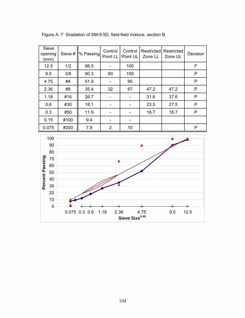
104

Figure A. 7 Gradation of SM-9.5D, field-field mixture, section B.

Sieve opening

(mm)Sieve # % Passing Control

Point LLControl

Point ULRestricted Zone LL

Restricted Zone UL Decision

12.5 1/2 98.5 - 100 F

9.5 3/8 90.3 90 100 P

4.75 #4 51.9 - 90 P

2.36 #8 35.4 32 67 47.2 47.2 P

1.18 #16 26.7 - - 31.6 37.6 P

0.6 #30 18.1 - - 23.5 27.5 P

0.3 #50 11.9 - - 18.7 18.7 P

0.15 #100 9.4 - -

0.075 #200 7.8 2 10 P

12.59.54.752.361.180.60.30.0750

102030405060708090

100

Sieve Size0.45

Perc

ent P

assi

ng

105

Figure A. 8 Gradation of SM-9.5D, field-lab mixture, section B.

Sieve opening

(mm)Sieve # % Passing Control

Point LLControl

Point ULRestricted Zone LL

Restricted Zone UL Decision

12.5 1/2 98.5 - 100 F

9.5 3/8 90.3 90 100 P

4.75 #4 51.9 - 90 P

2.36 #8 35.4 32 67 47.2 47.2 P

1.18 #16 26.7 - - 31.6 37.6 P

0.6 #30 18.1 - - 23.5 27.5 P

0.3 #50 11.9 - - 18.7 18.7 P

0.15 #100 9.4 - -

0.075 #200 7.8 2 10 P

12.59.54.752.361.180.60.30.0750

102030405060708090

100

Sieve Size0.45

Perc

ent P

assi

ng

106

Figure A. 9 Gradation of SM-9.5D, lab-lab mixture, section B.

Sieve opening

(mm)Sieve # % Passing Control

Point LLControl

Point ULRestricted Zone LL

Restricted Zone UL Decision

12.5 1/2 98.5 - 100 F

9.5 3/8 91.5 90 100 P

4.75 #4 58.8 - 90 P

2.36 #8 42.5 32 67 47.2 47.2 P

1.18 #16 30.8 - - 31.6 37.6 P

0.6 #30 22.9 - - 23.5 27.5 P

0.3 #50 15.1 - - 18.7 18.7 P

0.15 #100 11.1 - -

0.075 #200 8.7 2 10 P

12.59.54.752.361.180.60.30.0750

102030405060708090

100

Sieve Size0.45

Perc

ent P

assi

ng

107

Figure A. 10 Gradation of SM-9.5D, design-lab mixture, section B.

Sieve opening

(mm)Sieve # % Passing Control

Point LLControl

Point ULRestricted Zone LL

Restricted Zone UL Decision

12.5 1/2 99.7 - 100 F

9.5 3/8 86.1 90 100 F

4.75 #4 33.7 - 90 P

2.36 #8 22.9 32 67 47.2 47.2 F

1.18 #16 18.2 - - 31.6 37.6 P

0.6 #30 14.0 - - 23.5 27.5 P

0.3 #50 8.8 - - 18.7 18.7 P

0.15 #100 6.6 - -

0.075 #200 5.5 2 10 P

12.59.54.752.361.180.60.30.0750

102030405060708090

100

Sieve Size0.45

Perc

ent P

assi

ng

108

%#8 Quartzite Salem Stone Co., Sylvatus, VA 54

#10 Quartzite Salem Stone Co., Sylvatus, VA 21Concrete Sand Wythe Stone Co., Wytheville, VA 10

Fine RAP Adams Construction Co., Blacksburg, VA 15%

PG 76-22 Koch Materials Co., Pennsauken, NJ 5.8

%#8 Quartzite Salem Stone Co., Sylvatus, VA 52

#10 Quartzite Salem Stone Co., Sylvatus, VA 23Concrete Sand Wythe Stone Co., Wytheville, VA 10

Fine RAP Adams Construction Co., Blacksburg, VA 15%

PG 76-22 Koch Materials Co., Pennsauken, NJ 5.8

Design / Lab

Lab / Lab

Binder

Binder

Aggregate

Aggregate

Figure A. 11 Mixture designs for SM9.5E, section C.

109

Figure A. 12 Gradation of SM-9.5E, field-field mixture, section C.

Sieve opening

(mm)Sieve # % Passing Control

Point LLControl

Point ULRestricted Zone LL

Restricted Zone UL Decision

12.5 1/2 99.4 - 100 F

9.5 3/8 95.0 90 100 P

4.75 #4 61.7 - 90 P

2.36 #8 40.3 32 67 47.2 47.2 P

1.18 #16 29.2 - - 31.6 37.6 P

0.6 #30 22.6 - - 23.5 27.5 P

0.3 #50 15.3 - - 18.7 18.7 P

0.15 #100 10.7 - -

0.075 #200 8.2 2 10 P

12.59.54.752.361.180.60.30.0750

102030405060708090

100

Sieve Size0.45

Perc

ent P

assi

ng

110

Figure A. 13 Gradation of SM-9.5E, field-lab mixture, section C.

Sieve opening

(mm)Sieve # % Passing Control

Point LLControl

Point ULRestricted Zone LL

Restricted Zone UL Decision

12.5 1/2 98.0 - 100 F

9.5 3/8 90.9 90 100 P

4.75 #4 55.3 - 90 P

2.36 #8 34.3 32 67 47.2 47.2 P

1.18 #16 27.0 - - 31.6 37.6 P

0.6 #30 19.7 - - 23.5 27.5 P

0.3 #50 14.1 - - 18.7 18.7 P

0.15 #100 11.1 - -

0.075 #200 8.0 2 10 P

12.59.54.752.361.180.60.30.0750

102030405060708090

100

Sieve Size0.45

Perc

ent P

assi

ng

111

Figure A. 14 Gradation of SM-9.5E, lab-lab mixture, section C.

Sieve opening

(mm)Sieve # % Passing Control

Point LLControl

Point ULRestricted Zone LL

Restricted Zone UL Decision

12.5 1/2 99.7 - 100 F

9.5 3/8 90.2 90 100 P

4.75 #4 44.6 - 90 P

2.36 #8 35.2 32 67 47.2 47.2 P

1.18 #16 27.3 - - 31.6 37.6 P

0.6 #30 21.0 - - 23.5 27.5 P

0.3 #50 13.8 - - 18.7 18.7 P

0.15 #100 10.1 - -

0.075 #200 7.6 2 10 P

12.59.54.752.361.180.60.30.0750

102030405060708090

100

Sieve Size0.45

Perc

ent P

assi

ng

112

Figure A. 15 Gradation of SM-9.5E, design-lab mixture, section C.

Sieve opening

(mm)Sieve # % Passing Control

Point LLControl

Point ULRestricted Zone LL

Restricted Zone UL Decision

12.5 1/2 99.4 - 100 F

9.5 3/8 86.5 90 100 F

4.75 #4 44.9 - 90 P

2.36 #8 32.8 32 67 47.2 47.2 P

1.18 #16 25.2 - - 31.6 37.6 P

0.6 #30 19.3 - - 23.5 27.5 P

0.3 #50 12.5 - - 18.7 18.7 P

0.15 #100 8.9 - -

0.075 #200 6.6 2 10 P

12.59.54.752.361.180.60.30.0750

102030405060708090

100

Sieve Size0.45

Perc

ent P

assi

ng

113

%#8 Quartzite Salem Stone Co., Sylvatus, VA 50

#10 Quartzite Salem Stone Co., Sylvatus, VA 30Concrete Sand Wythe Stone Co., Wytheville, VA 10

Fine RAP Adams Construction Co., Blacksburg, VA 10%

PG 64-22 Associated Asphalt, Inc., Roanoke, VA 5.6

JMF %#8 Quartzite Salem Stone Co., Sylvatus, VA 50

#10 Quartzite Salem Stone Co., Sylvatus, VA 30Concrete Sand Wythe Stone Co., Wytheville, VA 10

Fine RAP Adams Construction Co., Blacksburg, VA 10%

PG 64-22 Associated Asphalt, Inc., Roanoke, VA 5.6?

Design / Lab

Binder

Binder

Lab / Lab

Aggregate

Aggregate

Figure A. 16 Mixture designs for SM-9.5A, section D.

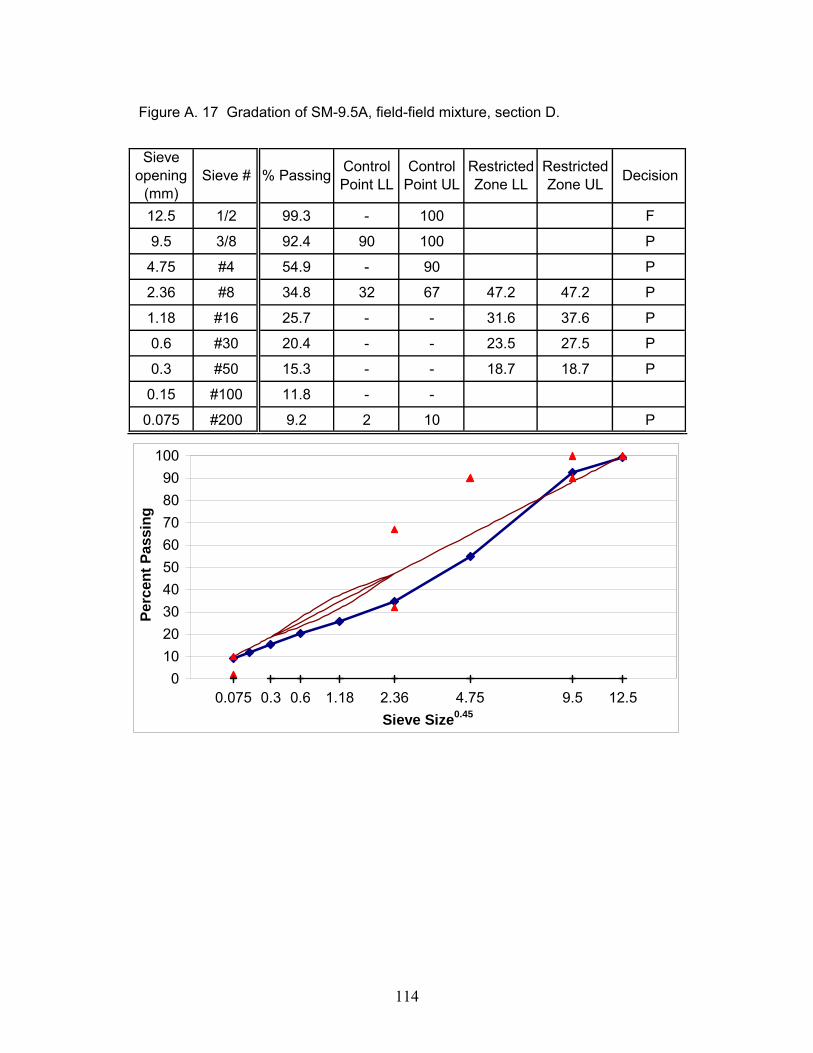
114

Figure A. 17 Gradation of SM-9.5A, field-field mixture, section D.

Sieve opening

(mm)Sieve # % Passing Control

Point LLControl

Point ULRestricted Zone LL

Restricted Zone UL Decision

12.5 1/2 99.3 - 100 F

9.5 3/8 92.4 90 100 P

4.75 #4 54.9 - 90 P

2.36 #8 34.8 32 67 47.2 47.2 P

1.18 #16 25.7 - - 31.6 37.6 P

0.6 #30 20.4 - - 23.5 27.5 P

0.3 #50 15.3 - - 18.7 18.7 P

0.15 #100 11.8 - -

0.075 #200 9.2 2 10 P

12.59.54.752.361.180.60.30.0750

102030405060708090

100

Sieve Size0.45

Perc

ent P

assi

ng

115

Figure A. 18 Gradation of SM-9.5A, field-lab mixture, section D.

Sieve opening

(mm)Sieve # % Passing Control

Point LLControl

Point ULRestricted Zone LL

Restricted Zone UL Decision

12.5 1/2 99.3 - 100 F

9.5 3/8 92.4 90 100 P

4.75 #4 54.9 - 90 P

2.36 #8 34.8 32 67 47.2 47.2 P

1.18 #16 25.7 - - 31.6 37.6 P

0.6 #30 20.4 - - 23.5 27.5 P

0.3 #50 15.3 - - 18.7 18.7 P

0.15 #100 11.8 - -

0.075 #200 9.2 2 10 P

12.59.54.752.361.180.60.30.0750

102030405060708090

100

Sieve Size0.45

Perc

ent P

assi

ng

116

Figure A.19 Gradation of SM-9.5A, lab-lab mixture, section D.

Sieve opening

(mm)Sieve # % Passing Control

Point LLControl

Point ULRestricted Zone LL

Restricted Zone UL Decision

12.5 1/2 100.0 - 100 P

9.5 3/8 89.3 90 100 F

4.75 #4 50.8 - 90 P

2.36 #8 37.0 32 67 47.2 47.2 P

1.18 #16 27.7 - - 31.6 37.6 P

0.6 #30 20.4 - - 23.5 27.5 P

0.3 #50 12.3 - - 18.7 18.7 P

0.15 #100 8.0 - -

0.075 #200 5.7 2 10 P

12.59.54.752.361.180.60.30.0750

102030405060708090

100

Sieve Size0.45

Perc

ent P

assi

ng

117

Figure A. 20 Gradation of SM-9.5A, design-lab mixture, section D.

Sieve opening

(mm)Sieve # % Passing Control

Point LLControl

Point ULRestricted Zone LL

Restricted Zone UL Decision

12.5 1/2 99.2 - 100 F

9.5 3/8 92.3 90 100 P

4.75 #4 58.3 - 90 P

2.36 #8 41.7 32 67 47.2 47.2 P

1.18 #16 28.7 - - 31.6 37.6 P

0.6 #30 20.3 - - 23.5 27.5 P

0.3 #50 12.4 - - 18.7 18.7 P

0.15 #100 8.6 - -

0.075 #200 6.3 2 10 P

12.59.54.752.361.180.60.30.0750

102030405060708090

100

Sieve Size0.45

Perc

ent P

assi

ng

118

%#8 Quartzite Salem Stone Co., Sylvatus, VA 60

#10 Limestone ACCO Stone Co., Blacksburg, VA 20Concrete Sand Wythe Stone Co., Wytheville, VA 10

Fine RAP Adams Construction Co., Blacksburg, VA 10%

PG 70-22 Associated Asphalt, Inc., Roanoke, VA 5.4

%#8 Quartzite Salem Stone Co., Sylvatus, VA 48

#10 Quartzite Salem Stone Co., Sylvatus, VA 12#10 Limestone ACCO Stone Co., Blacksburg, VA 20Concrete Sand Wythe Stone Co., Wytheville, VA 10

Fine RAP Adams Construction Co., Blacksburg, VA 10%

PG 70-22 Associated Asphalt, Inc., Roanoke, VA 5.8

Lab / Lab

Binder

Binder

Design / LabAggregate

Aggregate

Figure A. 21 Mixture designs for SM9.5D, setions E, F, G, and H.

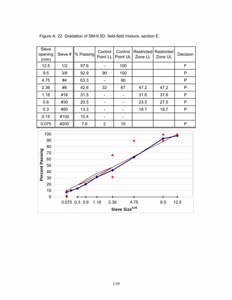
119

Figure A. 22 Gradation of SM-9.5D, field-field mixture, section E.

Sieve opening

(mm)Sieve # % Passing Control

Point LLControl

Point ULRestricted Zone LL

Restricted Zone UL Decision

12.5 1/2 97.6 - 100 F

9.5 3/8 92.9 90 100 P

4.75 #4 63.3 - 90 P

2.36 #8 42.6 32 67 47.2 47.2 P

1.18 #16 31.5 - - 31.6 37.6 P

0.6 #30 20.5 - - 23.5 27.5 P

0.3 #50 13.3 - - 18.7 18.7 P

0.15 #100 10.4 - -

0.075 #200 7.6 2 10 P

12.59.54.752.361.180.60.30.0750

102030405060708090

100

Sieve Size0.45

Perc

ent P

assi

ng

120

Figure A. 23 Gradation of SM-9.5D, field-lab mixture, section E.

Sieve opening

(mm)Sieve # % Passing Control

Point LLControl

Point ULRestricted Zone LL

Restricted Zone UL Decision

12.5 1/2 97.6 - 100 F

9.5 3/8 92.9 90 100 P

4.75 #4 63.3 - 90 P

2.36 #8 42.6 32 67 47.2 47.2 P

1.18 #16 31.5 - - 31.6 37.6 P

0.6 #30 20.5 - - 23.5 27.5 P

0.3 #50 13.3 - - 18.7 18.7 P

0.15 #100 10.4 - -

0.075 #200 7.6 2 10 P

12.59.54.752.361.180.60.30.0750

102030405060708090

100

Sieve Size0.45

Perc

ent P

assi

ng

121

Figure A. 24 Gradation of SM-9.5D, lab-lab mixture, section E.

Sieve opening

(mm)Sieve # % Passing Control

Point LLControl

Point ULRestricted Zone LL

Restricted Zone UL Decision

12.5 1/2 99.3 - 100 F

9.5 3/8 93.0 90 100 P

4.75 #4 61.4 - 90 P

2.36 #8 42.4 32 67 47.2 47.2 P

1.18 #16 31.0 - - 31.6 37.6 P

0.6 #30 23.0 - - 23.5 27.5 P

0.3 #50 15.2 - - 18.7 18.7 P

0.15 #100 11.1 - -

0.075 #200 8.5 2 10 P

12.59.54.752.361.180.60.30.0750

102030405060708090

100

Sieve Size0.45

Perc

ent P

assi

ng

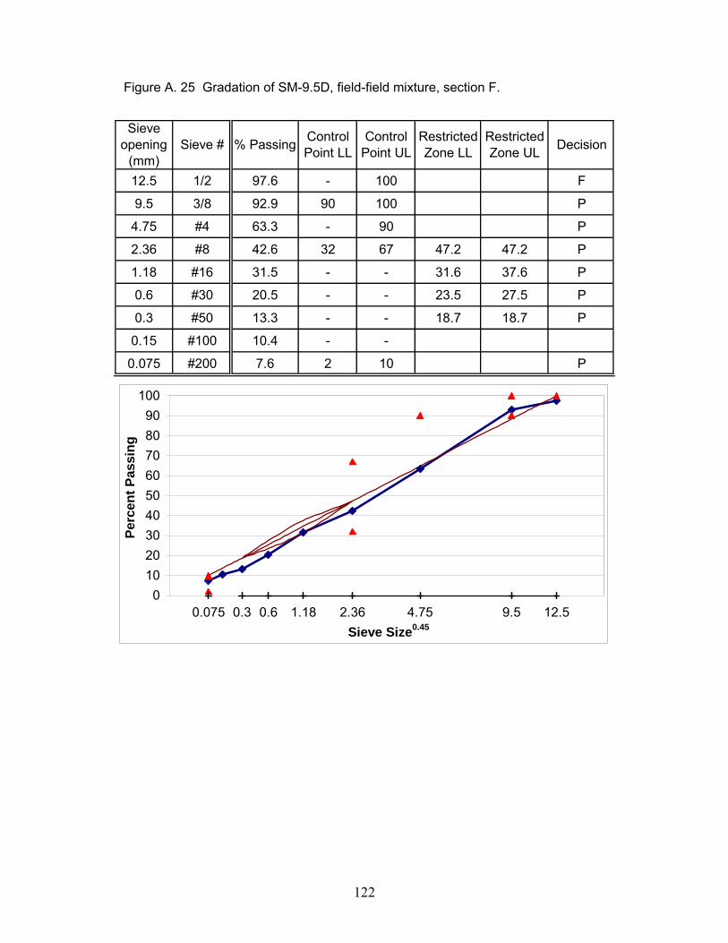
122

Figure A. 25 Gradation of SM-9.5D, field-field mixture, section F.

Sieve opening

(mm)Sieve # % Passing Control

Point LLControl

Point ULRestricted Zone LL

Restricted Zone UL Decision

12.5 1/2 97.6 - 100 F

9.5 3/8 92.9 90 100 P

4.75 #4 63.3 - 90 P

2.36 #8 42.6 32 67 47.2 47.2 P

1.18 #16 31.5 - - 31.6 37.6 P

0.6 #30 20.5 - - 23.5 27.5 P

0.3 #50 13.3 - - 18.7 18.7 P

0.15 #100 10.4 - -

0.075 #200 7.6 2 10 P

12.59.54.752.361.180.60.30.0750

102030405060708090

100

Sieve Size0.45

Perc

ent P

assi

ng

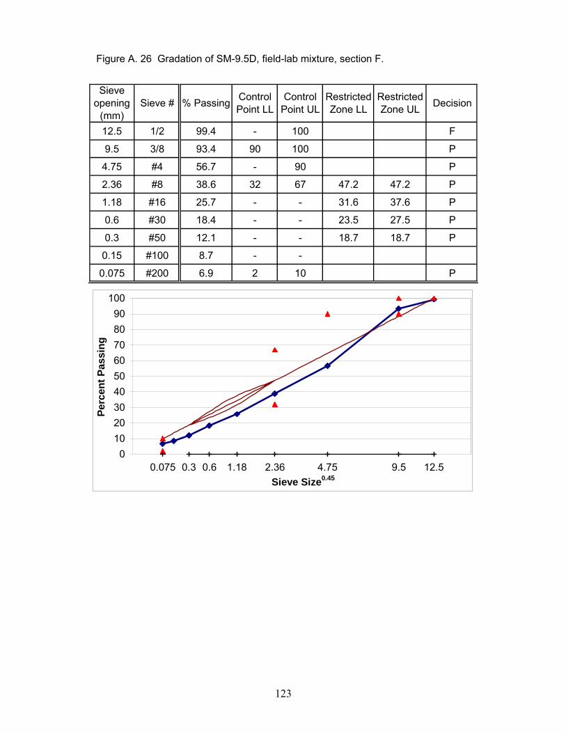
123

Figure A. 26 Gradation of SM-9.5D, field-lab mixture, section F.

Sieve opening

(mm)Sieve # % Passing Control

Point LLControl

Point ULRestricted Zone LL

Restricted Zone UL Decision

12.5 1/2 99.4 - 100 F

9.5 3/8 93.4 90 100 P

4.75 #4 56.7 - 90 P

2.36 #8 38.6 32 67 47.2 47.2 P

1.18 #16 25.7 - - 31.6 37.6 P

0.6 #30 18.4 - - 23.5 27.5 P

0.3 #50 12.1 - - 18.7 18.7 P

0.15 #100 8.7 - -

0.075 #200 6.9 2 10 P

12.59.54.752.361.180.60.30.0750

102030405060708090

100

Sieve Size0.45

Perc

ent P

assi

ng

124

Figure A. 27 Gradation of SM-9.5D, field-field mixture, section G.

Sieve opening

(mm)Sieve # % Passing Control

Point LLControl

Point ULRestricted Zone LL

Restricted Zone UL Decision

12.5 1/2 97.6 - 100 F

9.5 3/8 92.9 90 100 P

4.75 #4 63.3 - 90 P

2.36 #8 42.6 32 67 47.2 47.2 P

1.18 #16 31.5 - - 31.6 37.6 P

0.6 #30 20.5 - - 23.5 27.5 P

0.3 #50 13.3 - - 18.7 18.7 P

0.15 #100 10.4 - -

0.075 #200 7.6 2 10 P

12.59.54.752.361.180.60.30.0750

102030405060708090

100

Sieve Size0.45

Perc

ent P

assi

ng

125

Figure A. 28 Gradation of SM-9.5D, field-lab mixture, section G.

Sieve opening

(mm)Sieve # % Passing Control

Point LLControl

Point ULRestricted Zone LL

Restricted Zone UL Decision

12.5 1/2 98.4 - 100 F

9.5 3/8 95.1 90 100 P

4.75 #4 62.3 - 90 P

2.36 #8 42.2 32 67 47.2 47.2 P

1.18 #16 28.9 - - 31.6 37.6 P

0.6 #30 20.9 - - 23.5 27.5 P

0.3 #50 13.8 - - 18.7 18.7 P

0.15 #100 10.3 - -

0.075 #200 8.3 2 10 P

12.59.54.752.361.180.60.30.0750

102030405060708090

100

Sieve Size0.45

Perc

ent P

assi

ng

126

Figure A. 29 Gradation of SM-9.5D, field-field mixture, section H.

Sieve opening

(mm)Sieve # % Passing Control

Point LLControl

Point ULRestricted Zone LL

Restricted Zone UL Decision

12.5 1/2 98.3 - 100 F

9.5 3/8 94.3 90 100 P

4.75 #4 63.8 - 90 P

2.36 #8 43.1 32 67 47.2 47.2 P

1.18 #16 29.3 - - 31.6 37.6 P

0.6 #30 20.9 - - 23.5 27.5 P

0.3 #50 13.5 - - 18.7 18.7 P

0.15 #100 9.6 - -

0.075 #200 7.6 2 10 P

12.59.54.752.361.180.60.30.0750

102030405060708090

100

Sieve Size0.45

Perc

ent P

assi

ng

127

Figure A. 30 Gradation of SM-9.5D, field-lab mixture, section H.

Sieve opening

(mm)Sieve # % Passing Control

Point LLControl

Point ULRestricted Zone LL

Restricted Zone UL Decision

12.5 1/2 98.3 - 100 F

9.5 3/8 94.3 90 100 P

4.75 #4 63.8 - 90 P

2.36 #8 43.1 32 67 47.2 47.2 P

1.18 #16 29.3 - - 31.6 37.6 P

0.6 #30 20.9 - - 23.5 27.5 P

0.3 #50 13.5 - - 18.7 18.7 P

0.15 #100 9.6 - -

0.075 #200 7.6 2 10 P

12.59.54.752.361.180.60.30.0750

102030405060708090

100

Sieve Size0.45

Perc

ent P

assi

ng

128

Figure A. 31 Mixture design for SM-9.5A, section I.

%#8 Quartzite Salem Stone Co., Sylvatus, VA 50

#10 Quartzite Salem Stone Co., Sylvatus, VA 30Concrete Sand Wythe Stone Co., Wytheville, VA 10

Fine RAP Adams Construction Co., Blacksburg, VA 10%

PG 64-22 Associated Asphalt, Inc., Roanoke, VA 4.8

%#8 Quartzite Salem Stone Co., Sylvatus, VA 50

#10 Quartzite Salem Stone Co., Sylvatus, VA 30Concrete Sand Wythe Stone Co., Wytheville, VA 10

Fine RAP Adams Construction Co., Blacksburg, VA 10%

PG 64-22 Associated Asphalt, Inc., Roanoke, VA 5.04Binder

Binder

Design / Lab

Lab / Lab

Aggregate

Aggregate

129

Figure A. 32 Gradation of SM-9.5A, field-field mixture, section I.

Sieve opening

(mm)Sieve # % Passing Control

Point LLControl

Point ULRestricted Zone LL

Restricted Zone UL Decision

12.5 1/2 100.0 - 100 P

9.5 3/8 95.0 90 100 P

4.75 #4 51.8 - 90 P

2.36 #8 35.0 32 67 47.2 47.2 P

1.18 #16 27.8 - - 31.6 37.6 P

0.6 #30 20.6 - - 23.5 27.5 P

0.3 #50 13.9 - - 18.7 18.7 P

0.15 #100 10.6 - -

0.075 #200 7.3 2 10 P

12.59.54.752.361.180.60.30.0750

102030405060708090

100

Sieve Size0.45

Perc

ent P

assi

ng

130

Figure A. 33 Gradation of SM-9.5A, field-lab mixture, section I.

Sieve opening

(mm)Sieve # % Passing Control

Point LLControl

Point ULRestricted Zone LL

Restricted Zone UL Decision

12.5 1/2 100.0 - 100 P

9.5 3/8 95.0 90 100 P

4.75 #4 51.8 - 90 P

2.36 #8 35.0 32 67 47.2 47.2 P

1.18 #16 27.8 - - 31.6 37.6 P

0.6 #30 20.6 - - 23.5 27.5 P

0.3 #50 13.9 - - 18.7 18.7 P

0.15 #100 10.6 - -

0.075 #200 7.3 2 10 P

12.59.54.752.361.180.60.30.0750

102030405060708090

100

Sieve Size0.45

Perc

ent P

assi

ng

131

Figure A. 34 Gradation of SM-9.5A, lab-lab mixture, section I.

Sieve opening

(mm)Sieve # % Passing Control

Point LLControl

Point ULRestricted Zone LL

Restricted Zone UL Decision

12.5 1/2 99.4 - 100 F

9.5 3/8 92.7 90 100 P

4.75 #4 54.2 - 90 P

2.36 #8 37.6 32 67 47.2 47.2 P

1.18 #16 28.4 - - 31.6 37.6 P

0.6 #30 21.2 - - 23.5 27.5 P

0.3 #50 13.6 - - 18.7 18.7 P

0.15 #100 9.6 - -

0.075 #200 7.0 2 10 P

12.59.54.752.361.180.60.30.0750

102030405060708090

100

Sieve Size0.45

Perc

ent P

assi

ng

132

Figure A. 35 Gradation of SM-9.5A, design-lab mixture, section I.

Sieve opening

(mm)Sieve # % Passing Control

Point LLControl

Point ULRestricted Zone LL

Restricted Zone UL Decision

12.5 1/2 98.9 - 100 F

9.5 3/8 88.6 90 100 F

4.75 #4 56.7 - 90 P

2.36 #8 43.5 32 67 47.2 47.2 P

1.18 #16 31.0 - - 31.6 37.6 P

0.6 #30 22.1 - - 23.5 27.5 P

0.3 #50 13.9 - - 18.7 18.7 P

0.15 #100 10.1 - -

0.075 #200 7.6 2 10 P

12.59.54.752.361.180.60.30.0750

102030405060708090

100

Sieve Size0.45

Perc

ent P

assi

ng

133

Figure A. 36 Mixture design for SM-9.5D, section J.

%#8 Quartzite Salem Stone Co., Sylvatus, VA 48

#10 Quartzite Salem Stone Co., Sylvatus, VA 12#10 Limestone ACCO Stone Co., Blacksburg, VA 20Concrete Sand Wythe Stone Co., Wytheville, VA 10

Fine RAP Adams Construction Co., Blacksburg, VA 10%

PG 70-22 Associated Asphalt, Inc., Roanoke, VA 4.9

Aggregate

Binder

Lab / Lab

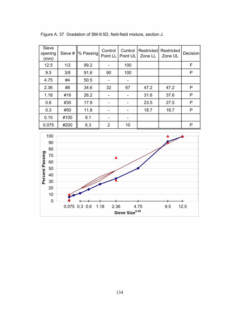
134

Figure A. 37 Gradation of SM-9.5D, field-field mixture, section J.

Sieve opening

(mm)Sieve # % Passing Control

Point LLControl

Point ULRestricted Zone LL

Restricted Zone UL Decision

12.5 1/2 99.2 - 100 F

9.5 3/8 91.6 90 100 P

4.75 #4 50.5 - -

2.36 #8 34.6 32 67 47.2 47.2 P

1.18 #16 26.2 - - 31.6 37.6 P

0.6 #30 17.9 - - 23.5 27.5 P

0.3 #50 11.8 - - 18.7 18.7 P

0.15 #100 9.1 - -

0.075 #200 6.3 2 10 P

12.59.54.752.361.180.60.30.0750

102030405060708090

100

Sieve Size0.45

Perc

ent P

assi

ng

135

Figure A. 38 Gradation of SM-9.5D, field-lab mixture, section J.

Sieve opening

(mm)Sieve # % Passing Control

Point LLControl

Point ULRestricted Zone LL

Restricted Zone UL Decision

12.5 1/2 99.2 - 100 F

9.5 3/8 91.6 90 100 P

4.75 #4 50.5 - -

2.36 #8 34.6 32 67 47.2 47.2 P

1.18 #16 26.2 - - 31.6 37.6 P

0.6 #30 17.9 - - 23.5 27.5 P

0.3 #50 11.8 - - 18.7 18.7 P

0.15 #100 9.1 - -

0.075 #200 6.3 2 10 P

12.59.54.752.361.180.60.30.0750

102030405060708090

100

Sieve Size0.45

Perc

ent P

assi

ng

136

Figure A. 39 Gradation of SM-9.5D, lab-lab mixture, section J.

Sieve opening

(mm)Sieve # % Passing Control

Point LLControl

Point ULRestricted Zone LL

Restricted Zone UL Decision

12.5 1/2 100.0 - 100 P

9.5 3/8 93.9 90 100 P

4.75 #4 52.9 - -

2.36 #8 31.6 32 67 47.2 47.2 F

1.18 #16 22.8 - - 31.6 37.6 P

0.6 #30 17.4 - - 23.5 27.5 P

0.3 #50 11.2 - - 18.7 18.7 P

0.15 #100 8.4 - -

0.075 #200 6.7 2 10 P

12.59.54.752.361.180.60.30.0750

102030405060708090

100

Sieve Size0.45

Perc

ent P

assi

ng

137

Figure A. 40 Mixture designs for SM-12.5A, section L.

%#68 Quartzite Salem Stone Co., Sylvatus, VA 26#8 Quartzite Salem Stone Co., Sylvatus, VA 55

#10 Quartzite Salem Stone Co., Sylvatus, VA 10Lime Filler James River Lime, Buchanan, VA 9

%PG 76-22 Koch Materials Co., Pennsauken, NJ 7.2

%Cellulose Hi-Tech Asphalt Solutions, Mechanicsville, VA 0.3

%#68 Quartzite Salem Stone Co., Sylvatus, VA 8#8 Quartzite Salem Stone Co., Sylvatus, VA 71

#10 Quartzite Salem Stone Co., Sylvatus, VA 12Lime Filler James River Lime, Buchanan, VA 9

%PG 76-22 Koch Materials Co., Pennsauken, NJ 6.8

%Cellulose Hi-Tech Asphalt Solutions, Mechanicsville, VA 0.3

Design / Lab

Lab / Lab

Aggregate

Binder

Fiber

Binder

Fiber

Aggregate

Note: Aggregate and binder percentages are by weight of mixture. Fiber percentages are by weight of binder.

138

Figure A. 41 Gradation of SM-12.5A, field-field mixture, section L.

Sieve opening

(mm)Sieve # % Passing Control

Point LLControl

Point ULRestricted Zone LL

Restricted Zone UL Decision

19 3/4 100.0 100 P

12.5 1/2 99.4 90 100 P

9.5 3/8 87.7 - 90 P

4.75 #4 36.8 - -

2.36 #8 25.0 28 58 39.1 39.1 F

1.18 #16 21.4 - - 25.6 31.6 P

0.6 #30 18.9 - - 19.1 23.1 P

0.3 #50 16.1 - - 15.5 15.5 P

0.15 #100 13.9 - -

0.075 #200 11.2 2 10 F

1912.59.54.752.361.180.60.30.0750

102030405060708090

100

Sieve Size0.45

Perc

ent P

assi

ng

139

Figure A. 42 Gradation of SM-12.5A, field-lab mixture, section L.

Sieve opening

(mm)Sieve # % Passing Control

Point LLControl

Point ULRestricted Zone LL

Restricted Zone UL Decision

19 3/4 100.0 100 P

12.5 1/2 99.4 90 100 P

9.5 3/8 87.7 - 90 P

4.75 #4 36.8 - -

2.36 #8 25.0 28 58 39.1 39.1 F

1.18 #16 21.4 - - 25.6 31.6 P

0.6 #30 18.9 - - 19.1 23.1 P

0.3 #50 16.1 - - 15.5 15.5 P

0.15 #100 13.9 - -

0.075 #200 11.2 2 10 F

1912.59.54.752.361.180.60.30.0750

102030405060708090

100

Sieve Size0.45

Perc

ent P

assi

ng

140

Figure A. 43 Gradation of SM-12.5A, lab-lab mixture, section L.

Sieve opening

(mm)Sieve # % Passing Control

Point LLControl

Point ULRestricted Zone LL

Restricted Zone UL Decision

19 3/4 100.0 100 P

12.5 1/2 92.8 90 100 P

9.5 3/8 76.3 - 90 P

4.75 #4 28.1 - -

2.36 #8 21.8 28 58 39.1 39.1 F

1.18 #16 17.9 - - 25.6 31.6 P

0.6 #30 15.3 - - 19.1 23.1 P

0.3 #50 14.0 - - 15.5 15.5 P

0.15 #100 13.1 - -

0.075 #200 11.7 2 10 F

1912.59.54.752.361.180.60.30.0750

102030405060708090

100

Sieve Size0.45

Perc

ent P

assi

ng

141

Figure A. 44 Gradation of SM-12.5A, design-lab mixture, section L.

Sieve opening

(mm)Sieve # % Passing Control

Point LLControl

Point ULRestricted Zone LL

Restricted Zone UL Decision

19 3/4 100.0 100 P

12.5 1/2 92.6 90 100 P

9.5 3/8 72.1 - 90 P

4.75 #4 27.8 - -

2.36 #8 19.5 28 58 39.1 39.1 F

1.18 #16 16.7 - - 25.6 31.6 P

0.6 #30 14.8 - - 19.1 23.1 P

0.3 #50 13.7 - - 15.5 15.5 P

0.15 #100 12.9 - -

0.075 #200 11.7 2 10 F

1912.59.54.752.361.180.60.30.0750

102030405060708090

100

Sieve Size0.45

Perc

ent P

assi

ng

142

Appendix B

Mixture Specifications and Volumetric Properties

143

Table B. 1 Volumetric properties for SM-12.5D mixtures, section A.

Property Field / Field Field / Lab Lab / Lab Design / Lab% Asphalt 5.86 5.86 5.93 5.55

Gmm 2.422 2.422 2.510 2.497Gmb 2.282 2.345 2.380 2.376Gb 1.03 1.03 1.03 1.03Gse 2.644 2.644 2.760 2.725Gsb 2.618 2.618 2.734 2.699CF 0.026 0.026 0.026 0.026

Bulk Density 142.4 146.3 148.5 148.3Density at Nini - 134.2 134.0 133.1

% passing #200 5.64 5.64 12.28 5.96

Table B. 2 VDOT specifications for SM-12.5D mixtures, section A.

Min. Max.VTM (%) 2.5 5.5 5.8 Fail 3.2 Pass 5.2 Pass 4.8 PassVMA (%) 12 - 18.0 Pass 15.7 Pass 18.1 Pass 16.8 PassVFA (%) 62 80 67.8 Pass 79.8 Pass 71.4 Pass 71.4 Pass

% Density at Nini - 89 - - 88.8 Pass 85.6 Pass 85.5 PassF/A ratio 0.6 1.3 1.0 Pass 1.0 Pass 2.2 Fail 1.1 Pass

Property Field / Lab Lab / Lab Design / LabField / FieldSpecification

144

Table B. 3 Volumetric properties for SM-9.5D mixtures, section B.

Property Field / Field Field / Lab Lab / Lab Design / Lab% Asphalt 4.71 4.71 5.36 5.33

Gmm 2.450 2.450 2.513 2.494Gmb 2.239 2.362 2.468 2.370Gb 1.03 1.03 1.03 1.03Gse 2.629 2.629 2.736 2.711Gsb 2.574 2.574 2.681 2.656CF 0.055 0.055 0.055 0.055

Bulk Density 139.7 147.4 154.0 147.9Density at Nini - 135.1 141.7 133.1

% passing #200 7.81 7.81 8.72 5.52

Table B. 4 VDOT specifications for SM-9.5D mixtures, section B.

Min. Max.VTM (%) 2.5 5.5 8.6 Fail 3.6 Pass 1.8 Fail 5.0 PassVMA (%) 12 - 17.1 Pass 12.5 Pass 12.9 Pass 15.5 PassVFA (%) 62 80 49.7 Fail 71.6 Pass 86.0 Fail 68.0 Pass

% Density at Nini - 89 - - 88.4 Pass 90.4 Fail 85.6 PassF/A ratio 0.6 1.3 2.0 Fail 2.0 Fail 1.9 Fail 1.2 Pass

Property Field / Lab Lab / Lab Design / LabField / FieldSpecification

145

Table B. 6 VDOT specifications for SM-12.5E mixtures, section C.

Min. Max.VTM (%) 2.5 5.5 6.0 Fail 2.3 Fail 2.0 Fail 1.3 FailVMA (%) 12 - 18.1 Pass 14.9 Pass 15.3 Pass 14.9 PassVFA (%) 62 80 67.0 Pass 84.6 Fail 86.6 Fail 91.4 Fail

% Density at Nini - 89 - - 89.7 Fail 89.9 Fail 89.4 FailF/A ratio 0.6 1.3 1.5 Fail 1.5 Fail 1.3 Pass 1.1 Pass

Property Field / Lab Lab / Lab Design / LabField / FieldSpecification

Table B. 5 Volumetric properties for SM-9.5E mixtures, section C.

Property Field / Field Field / Lab Lab / Lab Design / Lab% Asphalt 5.80 5.80 6.02 6.16

Gmm 2.455 2.455 2.477 2.463Gmb 2.309 2.399 2.426 2.431Gb 1.03 1.03 1.03 1.03Gse 2.684 2.684 2.721 2.711Gsb 2.654 2.654 2.691 2.681CF 0.03 0.03 0.03 0.03

Bulk Density 144.1 149.7 151.4 151.7Density at Nini - 137.5 139.0 137.4

% passing #200 8.18 8.03 7.56 6.60

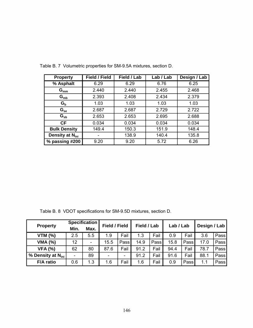
146

Table B. 7 Volumetric properties for SM-9.5A mixtures, section D.

Property Field / Field Field / Lab Lab / Lab Design / Lab% Asphalt 6.29 6.29 6.76 6.25

Gmm 2.440 2.440 2.455 2.468Gmb 2.393 2.408 2.434 2.379Gb 1.03 1.03 1.03 1.03Gse 2.687 2.687 2.729 2.722Gsb 2.653 2.653 2.695 2.688CF 0.034 0.034 0.034 0.034

Bulk Density 149.4 150.3 151.9 148.4Density at Nini - 138.9 140.4 135.8

% passing #200 9.20 9.20 5.72 6.26

Table B. 8 VDOT specifications for SM-9.5D mixtures, section D.

Min. Max.VTM (%) 2.5 5.5 1.9 Fail 1.3 Fail 0.9 Fail 3.6 PassVMA (%) 12 - 15.5 Pass 14.9 Pass 15.8 Pass 17.0 PassVFA (%) 62 80 87.6 Fail 91.2 Fail 94.4 Fail 78.7 Pass

% Density at Nini - 89 - - 91.2 Fail 91.6 Fail 88.1 PassF/A ratio 0.6 1.3 1.6 Fail 1.6 Fail 0.9 Pass 1.1 Pass

Property Field / Lab Lab / Lab Design / LabField / FieldSpecification

147

Table B. 9 Volumetric properties for SM-9.5D mixtures, section E.

Property Field / Field Field / Lab Lab / Lab% Asphalt 5.85 5.85 6.00

Gmm 2.434 2.434 2.489Gmb 2.317 2.400 2.442Gb 1.03 1.03 1.03Gse 2.659 2.659 2.737Gsb 2.604 2.604 2.682CF 0.055 0.055 0.055

Bulk Density 144.6 149.8 152.4Density at Nini - 137.3 140.2

% passing #200 7.57 7.57 8.47

Table B. 10 VDOT specifications for SM-9.5D mixtures, section E.

Min. Max.VTM (%) 2.5 5.5 4.8 Pass 1.4 Fail 1.9 FailVMA (%) 12 - 16.2 Pass 13.2 Pass 14.4 PassVFA (%) 62 80 70.5 Pass 89.6 Fail 86.8 Fail

% Density at Nini - 89 - - 90.4 Fail 90.2 FailF/A ratio 0.6 1.3 1.5 Fail 1.5 Fail 1.6 Fail

Property Field / Lab Lab / LabField / FieldSpecification

148

Table B. 11 Volumetric properties for SM-9.5D mixtures, section F.

Property Field / Field Field / Lab% Asphalt 5.85 5.42

Gmm 2.434 2.502Gmb 2.317 2.412Gb 1.03 1.03Gse 2.659 2.725Gsb 2.604 2.670CF 0.055 0.055

Bulk Density 144.6 150.5Density at Nini - 137.5

% passing #200 7.57 6.88

Table B. 12 VDOT specifications for SM-9.5D mixtures, section F.

Min. Max.VTM (%) 2.5 5.5 4.8 Pass 3.6 PassVMA (%) 12 - 16.2 Pass 14.5 PassVFA (%) 62 80 70.5 Pass 75.4 Pass

% Density at Nini - 89 - - 88.1 PassF/A ratio 0.6 1.3 1.5 Fail 1.5 Fail

Property Field / LabField / FieldSpecification

149

Table B. 13 Volumetric properties for SM-9.5D mixtures, section G.

Property Field / Field Field / Lab% Asphalt 5.85 6.29

Gmm 2.434 2.499Gmb 2.317 2.410Gb 1.03 1.03Gse 2.659 2.763Gsb 2.604 2.708CF 0.055 0.055

Bulk Density 144.6 150.4Density at Nini - 137.6

% passing #200 7.57 8.35

Table B. 14 VDOT specifications for SM-9.5D mixtures, section G.

Min. Max.VTM (%) 2.5 5.5 4.8 Pass 3.6 PassVMA (%) 12 - 16.2 Pass 16.6 PassVFA (%) 62 80 70.5 Pass 78.6 Pass

% Density at Nini - 89 - - 88.2 PassF/A ratio 0.6 1.3 1.5 Fail 1.5 Fail

Property Field / LabField / FieldSpecification

150

Table B. 15 Volumetric properties for SM-9.5D mixtures, section H.

Property Field / Field Field / Lab% Asphalt 5.85 5.63

Gmm 2.434 2.507Gmb 2.317 2.403Gb 1.03 1.03Gse 2.659 2.741Gsb 2.604 2.686CF 0.055 0.055

Bulk Density 144.6 149.9Density at Nini - 137.4

% passing #200 7.57 7.57

Table B. 16 VDOT specifications for SM-9.5D mixtures, section H.

Min. Max.VTM (%) 2.5 5.5 4.8 Pass 4.1 PassVMA (%) 12 - 16.2 Pass 15.6 PassVFA (%) 62 80 70.5 Pass 73.4 Pass

% Density at Nini - 89 - - 87.8 PassF/A ratio 0.6 1.3 1.5 Fail 1.5 Fail

Property Field / LabField / FieldSpecification

151

Table B. 17 Volumetric properties for SM-9.5A mixtures, section I.

Property Field / Field Field / Lab Lab / Lab Design / Lab% Asphalt 5.42 5.42 5.31 5.37

Gmm 2.467 2.467 2.489 2.498Gmb 2.440 2.429 2.340 2.390Gb 1.03 1.03 1.03 1.03Gse 2.681 2.681 2.704 2.718Gsb 2.647 2.647 2.670 2.684CF 0.034 0.034 0.034 0.034

Bulk Density 152.3 151.6 146.0 149.1Density at Nini - 138.1 133.4 137.0

% passing #200 7.27 7.27 6.97 7.64

Table B. 18 VDOT specifications for SM-9.5A mixtures, section I.

Min. Max.VTM (%) 2.5 5.5 1.1 Fail 1.5 Fail 6.0 Fail 4.3 PassVMA (%) 12 - 12.8 Pass 13.2 Pass 17.0 Pass 15.7 PassVFA (%) 62 80 91.6 Fail 88.5 Fail 64.8 Pass 72.5 Pass

% Density at Nini - 89 - - 89.8 Fail 85.9 Pass 87.9 PassF/A ratio 0.6 1.3 1.5 Fail 1.5 Fail 1.4 Fail 1.6 Fail

Property Field / Lab Lab / Lab Design / LabField / FieldSpecification

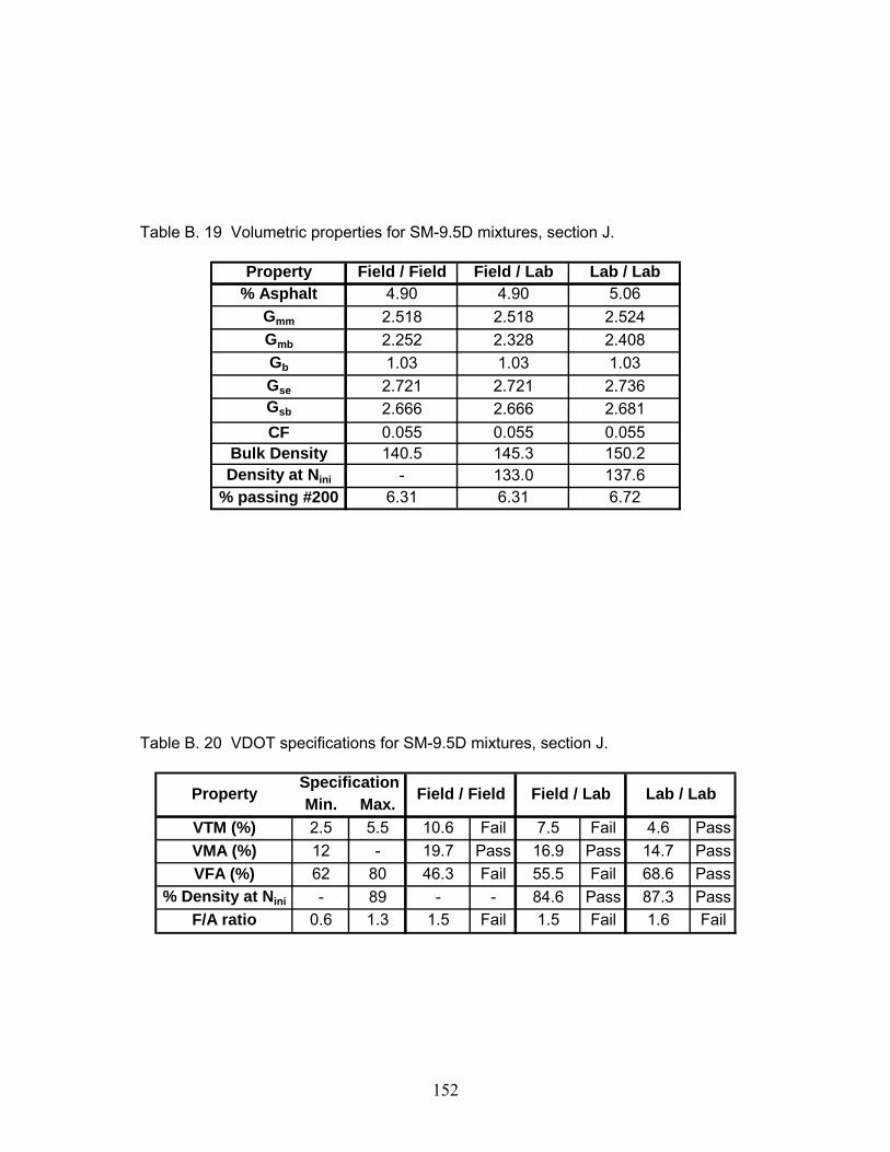
152

Table B. 19 Volumetric properties for SM-9.5D mixtures, section J.

Property Field / Field Field / Lab Lab / Lab% Asphalt 4.90 4.90 5.06

Gmm 2.518 2.518 2.524Gmb 2.252 2.328 2.408Gb 1.03 1.03 1.03Gse 2.721 2.721 2.736Gsb 2.666 2.666 2.681CF 0.055 0.055 0.055

Bulk Density 140.5 145.3 150.2Density at Nini - 133.0 137.6

% passing #200 6.31 6.31 6.72

Table B. 20 VDOT specifications for SM-9.5D mixtures, section J.

Min. Max.VTM (%) 2.5 5.5 10.6 Fail 7.5 Fail 4.6 PassVMA (%) 12 - 19.7 Pass 16.9 Pass 14.7 PassVFA (%) 62 80 46.3 Fail 55.5 Fail 68.6 Pass

% Density at Nini - 89 - - 84.6 Pass 87.3 PassF/A ratio 0.6 1.3 1.5 Fail 1.5 Fail 1.6 Fail

Property Field / Lab Lab / LabField / FieldSpecification

153

Table B. 21 Volumetric properties for SM-12.5A mixtures, section L.

Property Field / Field Field / Lab Lab / Lab Design / Lab% Asphalt 6.80 6.80 6.44 6.33

Gmm 2.402 2.402 2.402 2.415Gmb 2.226 2.359 2.359 2.359Gb 1.03 1.03 1.03 1.03Gse 2.661 2.661 2.644 2.657Gsb 2.631 2.631 2.614 2.627CF 0.03 0.03 0.03 0.03

Bulk Density 138.9 147.2 147.2 147.2Density at Nini - 134.5 134.1 132.0

% passing #200 11.25 11.25 11.71 11.67

Table B. 22 VDOT specifications for SM-12.5A mixtures, section L.

Min. Max.VTM (%) 2.5 5.5 7.3 Fail 1.8 Fail 1.8 Fail 2.3 FailVMA (%) 12 21.1 Pass 16.4 Pass 15.6 Pass 15.9 PassVFA (%) 62 80 65.3 Pass 89.0 Fail 88.5 Fail 85.3 Fail

% Density at Nini - 89 - - 89.7 Fail 89.5 Fail 87.6 PassF/A ratio 0.6 1.3 1.8 Fail 1.8 Fail 1.9 Fail 2.0 Fail

Property Field / Lab Lab / Lab Design / LabField / FieldSpecification

154

Appendix C

Indirect Tensile Strength

155

F/L 100-mm Diameter Specimens

Sample Thickness Load, N strength*E-3,

kN/mm2 Average Std Dev Average (Mr,

creep) Std Dev (Mr,

Creep) A1-4in-

FL 63.57 18245 1.827 A2-4in-

FL broken - - A3-4in-

FL 62.76 18606 1.887

1.926 0.123

A4-4in-FL 61.42 19891 2.062

A5-4in-FL 63.31 20521 2.063

A6-4in-FL 62.67 19613 1.992

1.966 0.106

2.027 0.049

B1-4in-FL 63.31 21590 2.171

B2-4in-FL 62.95 20748 2.098

B3-4in-FL 63.41 19012 1.909

2.060 0.135

B4-4in-FL 64.14 22471 2.230

B5-4in-FL 62.21 20512 2.099

B6-4in-FL 61.56 19272 1.993

2.083 0.117

2.107 0.119

C1-4in-FL 63.21 23552 2.372

C2-4in-FL 64.52 26867 2.651

C3-4in-FL 64.42 23785 2.351

2.355 0.015

C4-4in-FL 63.81 25795 2.574

C5-4in-FL 62.21 22892 2.343

C6-4in-FL 62.87 24809 2.512

2.467 0.131

2.579 0.070

D1-4in-FL 62.04 19511 2.002

D2-4in-FL 62.54 23003 2.342

D3-4in-FL 64.37 20658 2.043

2.076 0.095

D4-4in-FL 62.57 23271 2.368

D5-4in-FL 62.42 21414 2.184

D6-4in-FL 63.68 23176 2.317

2.209 0.159

2.342 0.026

156

Sample Thickness Load, N strength*E-3,

kN/mm2 Average Std Dev Average (Mr,

creep) Std Dev (Mr,

Creep) E1-4in-

FL 62.53 19687 2.004 E2-4in-

FL 63.34 22071 2.218 E3-4in-

FL 62.53 19287 1.964

2.029 0.080

E4-4in-FL 63.15 22235 2.242

E5-4in-FL 63.10 20993 2.118

E6-4in-FL 63.32 22286 2.241

2.131 0.123

2.234 0.014

F1-4in-FL 63.86 21566 2.150

F2-4in-FL 63.64 24627 2.464

F3-4in-FL 62.45 19825 2.021

2.128 0.098

F4-4in-FL 64.64 24579 2.421

F5-4in-FL 62.70 21805 2.214

F6-4in-FL 62.62 23385 2.377

2.275 0.174

2.421 0.044

G1-4in-FL 62.23 20873 2.135

G2-4in-FL 63.04 23212 2.344

G3-4in-FL 64.06 21441 2.131

2.089 0.076

G4-4in-FL 64.30 23370 2.314

G5-4in-FL 64.32 20216 2.001

G6-4in-FL 63.44 22387 2.247

2.195 0.130

2.302 0.050

H1-4in-FL 62.48 18624 1.898

H2-4in-FL 66.25 24000 2.306

H3-4in-FL 62.64 21229 2.157

2.021 0.130

H4-4in-FL 63.15 22528 2.271

H5-4in-FL 60.93 19231 2.009

H6-4in-FL 63.20 23077 2.325

2.161 0.175

2.301 0.027

157

Sample Thickness Load, N strength*E-3,

kN/mm2 Average Std Dev Average (Mr,

creep) Std Dev (Mr,

Creep) I1-4in-

FL 63.52 23098 2.315 I2-4in-

FL 63.60 26936 2.696 I3-4in-

FL 63.60 24048 2.407

2.431 0.130

I4-4in-FL 64.13 26180 2.599

I5-4in-FL 64.50 26055 2.572

I6-4in-FL 64.27 26566 2.631

2.537 0.145

2.642 0.049

J1-4in-FL 63.84 18418 1.837

J2-4in-FL 63.24 18830 1.896

J3-4in-FL 64.74 17946 1.765

1.834 0.068

J4-4in-FL 63.31 19386 1.949

J5-4in-FL 64.74 19332 1.901

J6-4in-FL 64.41 19813 1.958

1.884 0.073

1.934 0.034

L1-4in-FL 65.29 17241 1.681

L2-4in-FL 62.75 19852 2.014

L3-4in-FL 62.64 18379 1.868

1.779 0.094

L4-4in-FL 64.91 19905 1.952

L5-4in-FL 61.71 17322 1.787

L6-4in-FL 61.50 20586 2.131

1.906 0.162

2.032 0.091

158

L/L 100-mm Diameter Specimens

Sample Thickness Load, N strength*E-3,

kN/mm2 Average Std Dev Average (Mr,

creep) Std Dev (Mr,

Creep) A1-4in-

LL 63.20 23445 2.362 A2-4in-

LL 65.20 28041 2.738 A3-4in-

LL 63.47 24854 2.493

2.494 0.133

A4-4in-LL 64.67 26801 2.638

A5-4in-LL 64.85 26769 2.628

A6-4in-LL 64.33 25944 2.567

2.571 0.131

2.648 0.086

B1-4in-LL 63.16 26150 2.636

B2-4in-LL 63.20 23749 2.392

B3-4in-LL 62.48 23212 2.365

2.552 0.163

B4-4in-LL 64.77 24517 2.410

B5-4in-LL 66.45 27718 2.656

B6-4in-LL 61.90 23976 2.466

2.488 0.127

2.423 0.039

C1-4in-LL 63.22 29239 2.944

C2-4in-LL 61.80 29140 3.002

C3-4in-LL 62.38 29600 3.021

2.989 0.040

C4-4in-LL 58.73 26855 2.911

C5-4in-LL 63.34 29869 3.002

C6-4in-LL 61.07 27691 2.887

2.961 0.055

2.933 0.061

D1-4in-LL 65.19 22289 2.177

D2-4in-LL 64.50 20500 2.023

D3-4in-LL 64.77 23582 2.318

2.280 0.090

D4-4in-LL 64.93 22020 2.159

D5-4in-LL 63.87 23531 2.345

D6-4in-LL 62.43 21282 2.170

2.199 0.118

2.117 0.082

159

Sample Thickness Load, N strength*E-3,

kN/mm2 Average Std Dev Average (Mr,

creep) Std Dev (Mr,

Creep) E1-4in-

LL 61.30 20873 2.168 E2-4in-

LL 65.30 21611 2.107 E3-4in-

LL 64.37 23122 2.287

2.262 0.084

E4-4in-LL 61.93 21456 2.206

E5-4in-LL 60.57 22175 2.331

E6-4in-LL 59.93 20592 2.187

2.214 0.082

2.167 0.053

I1-4in-LL 65.20 23006 2.246

I2-4in-LL 64.63 230068 2.272

I3-4in-LL 64.26 23206 2.299

2.323 0.091

I4-4in-LL 63.80 22172 2.212

I5-4in-LL 64.63 24597 2.423

I6-4in-LL 64.77 24069 2.366

2.303 0.079

2.283 0.078

J1-4in-LL 62.56 20760 2.113

J2-4in-LL 62.17 20473 2.096

J3-4in-LL 64.42 18750 1.853

1.990 0.131

J4-4in-LL 64.77 18672 1.835

J5-4in-LL 64.37 20267 2.004

J6-4in-LL 63.83 20715 2.066

1.995 0.122

1.999 0.143

L1-4in-LL 63.78 15898 1.587

L2-4in-LL 63.77 15494 1.547

L3-4in-LL 64.58 16602 1.637

1.664 0.094

L4-4in-LL 62.83 16110 1.632

L5-4in-LL 64.52 17928 1.769

L6-4in-LL 64.37 17672 1.748

1.653 0.088

1.642 0.101

160

D/L 100-mm Diameter Specimens

Sample Thickness Load, N strength*E-3,

kN/mm2 Average Std Dev Average (Mr,

creep) Std Dev (Mr,

Creep) A1-4in-

DL 63.00 19213 1.941 A2-4in-

DL 63.07 19228 1.941 A3-4in-

DL 63.72 19508 1.949

1.988 0.075

A4-4in-DL 63.23 19463 1.960

A5-4in-DL 63.36 20649 2.075

A6-4in-DL 62.43 19684 2.007

1.979 0.053

1.969 0.034

B1-4in-DL 62.61 15485 1.575

B2-4in-DL 64.00 15927 1.584

B3-4in-DL 63.96 17630 1.755

1.681 0.094

B4-4in-DL 63.10 16949 1.710

B5-4in-DL 65.42 17606 1.713

B6-4in-DL 63.90 16241 1.618

1.659 0.076

1.637 0.065

C1-4in-DL 63.27 26267 2.643

C2-4in-DL 63.27 25505 2.566

C3-4in-DL 63.64 26640 2.665

2.642 0.024

C4-4in-DL 63.30 24606 2.475

C5-4in-DL 63.76 26210 2.617

C6-4in-DL 63.77 24146 2.411

2.563 0.101

2.484 0.078

161

Sample Thickness Load, N strength*E-3,

kN/mm2 Average Std Dev Average (Mr,

creep) Std Dev (Mr,

Creep) D1-4in-

DL 64.46 24338 2.404 D2-4in-

DL 63.47 22973 2.304 D3-4in-

DL 63.58 25204 2.524

2.424 0.092

D4-4in-DL 64.70 23185 2.281

D5-4in-DL 64.30 23669 2.343

D6-4in-DL 64.93 24427 2.395

2.375 0.088

2.327 0.060

I1-4in-DL 63.57 33700 3.375

I2-4in-DL 63.30 30439 3.061

I3-4in-DL 63.38 31165 3.130

3.253 0.123

I4-4in-DL 63.70 31867 3.185

I5-4in-DL 62.20 31789 3.254

I6-4in-DL 62.00 29946 3.075

3.180 0.119

3.107 0.068

L1-4in-DL 66.08 20368 1.962

L2-4in-DL 65.50 18854 1.833

L3-4in-DL 62.79 18367 1.862

1.932 0.061

L4-4in-DL 62.33 18430 1.882

L5-4in-DL 61.93 19198 1.973

L6-4in-DL 65.23 19180 1.872

1.897 0.057

1.862 0.026

162

Vitae

Samer Katicha was born on May the 11, 1976 in Beirut, Lebanon. He received his

high school diplomat from the “College Notre Dame de Jamhour” in 1994. After that he

joined the American University of Beirut where he received his bachelor in engineering

(BE) in 1999. After graduation, Samer served as an engineer in the military, as part of a

required one year military service. In August 2000, he decided to go back to school by

entering the graduate program at the Charles E Via Department of Civil and

Environmental Engineering at Virginia Tech which earned him a Masters degree in 2003

under the supervision of Dr. Imad Al-Qadi. During the same period samer worked as a

Graduate Research Assistant with the Roadway Infrastructure Group (RIG) at the

Virginia Tech Transportation Institute. Currently, Samer is pursuing a Ph. D. degree

under the supervision of Dr. Imad Al-Qadi.