Development of Effective Approaches to the Large-Scale

Florida International UniversityFIU Digital Commons

FIU Electronic Theses and Dissertations University Graduate School

11-6-2013

Development of Effective Approaches to the Large-Scale Aerodynamic Testing of Low-Rise BuildingTuan-Chun [email protected]

Follow this and additional works at: https://digitalcommons.fiu.edu/etdPart of the Civil Engineering Commons, Fluid Dynamics Commons, and the Structural

Engineering Commons

This work is brought to you for free and open access by the University Graduate School at FIU Digital Commons. It has been accepted for inclusion inFIU Electronic Theses and Dissertations by an authorized administrator of FIU Digital Commons. For more information, please contact [email protected].

Recommended CitationFu, Tuan-Chun, "Development of Effective Approaches to the Large-Scale Aerodynamic Testing of Low-Rise Building" (2013). FIUElectronic Theses and Dissertations. 986.https://digitalcommons.fiu.edu/etd/986

https://digitalcommons.fiu.edu/?utm_source=digitalcommons.fiu.edu%2Fetd%2F986&utm_medium=PDF&utm_campaign=PDFCoverPages

https://digitalcommons.fiu.edu/etd?utm_source=digitalcommons.fiu.edu%2Fetd%2F986&utm_medium=PDF&utm_campaign=PDFCoverPages

https://digitalcommons.fiu.edu/ugs?utm_source=digitalcommons.fiu.edu%2Fetd%2F986&utm_medium=PDF&utm_campaign=PDFCoverPages

https://digitalcommons.fiu.edu/etd?utm_source=digitalcommons.fiu.edu%2Fetd%2F986&utm_medium=PDF&utm_campaign=PDFCoverPages

http://network.bepress.com/hgg/discipline/252?utm_source=digitalcommons.fiu.edu%2Fetd%2F986&utm_medium=PDF&utm_campaign=PDFCoverPages




https://digitalcommons.fiu.edu/etd/986?utm_source=digitalcommons.fiu.edu%2Fetd%2F986&utm_medium=PDF&utm_campaign=PDFCoverPages

mailto:[email protected]

FLORIDA INTERNATIONAL UNIVERSITY

Miami, Florida

DEVELOPMENT OF EFFECTIVE APPROACHES TO THE LARGE-SCALE AERO-

DYNAMIC TESTING OF LOW-RISE BUILDINGS

A dissertation submitted in partial fulfillment of the

requirements for the degree of

DOCTOR OF PHILOSOPHY

in

CIVIL ENGINEERING

by

Tuan-Chun Fu

2013

ii

To: Dean Amir Mirmiran College of Engineering and Computing

This dissertation, written by Tuan-Chun Fu, and entitled Development of Effective Ap-proaches to the Large-Scale Aerodynamic Testing of Low-Rise Building, having been approved in respect to style and intellectual content, is referred to you for judgment.

We have read this dissertation and recommend that it be approved.

________________________________________ Girma Bitsuamlak

________________________________________

Nakin Suksawang

________________________________________ Yimin Zhu

________________________________________

Arindam Gan Chowdhury, Major Professor

Date of Defense: November 6, 2013

The dissertation of Tuan-Chun Fu is approved.

________________________________________ Dean Amir Mirmiran

College of Engineering and Computing

________________________________________ Dean Lakshmi N. Reddi

University Graduate School

Florida International University, 2013

iii

© Copyright 2013 by Tuan-Chun Fu

All rights reserved.

iv

DEDICATION

I dedicate this dissertation to my wonderful family, especially my parents and my

wife for encouraging me to pursue my dreams and supporting me in every way for all

these years. Thank you for all of your love, patience and sacrifice.

v

ACKNOWLEDGMENTS

First and foremost I would like to thank my advisor, Dr. Arindam Gan Chow-

dhury. I appreciate all his contributions of time, ideas, and funding to make my Ph.D. ex-

perience productive and stimulating. I also would like to express my gratitude to, Dr. Pe-

ter Irwin, Dr. Emil Simiu, and Dr. Ruilong Li for their advice and guidance from the very

early stage of this research and to Mr. Walter Conklin, Mr. James Erwin, and Mr. Roy

Liu for their technical support. I would like to thank my committee members, Dr. Grima

Bitsuamlak, Dr. Nakin Suksawang, and Dr. Yimin Zhu, for their suggestions and help

with my dissertation, for their time, interests, and thought provocative questions.

The Wall of Wind research performed was supported by the National Science

Foundation (NSF Award No. CMMI-0928740 and CMMI-1151003), Florida Sea Grant

College Program (Project # R/C-D-19-FIU), and Center of Excellence in Hurricane Dam-

age Mitigation and Product Development. WOW instrumentation has been supported

through the NSF MRI Award No. CMMI-0923365. The support from the Department of

Energy, Florida Division of Emergency Management, Renaissance Re, Roofing Alliance

for Progress, and AIR Worldwide is acknowledged. The collaboration from RWDI USA

LLC in terms of performing the wind tunnel tests is greatly appreciated.

Finally, I take this opportunity to express my profound gratitude to my family for

their unconditional love and encouragement. My parents, Mr. John Fu and Miss Nancy

Wu, and my wife, Miss Cathy Chen always supported my endeavors with great enthusi-

asm.

vi

ABSTRACT OF THE DISSERTATION

DEVELOPMENT OF EFFECTIVE APPROACHES TO THE LARGE-SCALE AERO-

DYNAMIC TESTING OF LOW-RISE BUILDINGS

by

Tuan-Chun Fu

Florida International University, 2013

Miami, Florida

Professor Arindam Gan Chowdhury, Major Professor

Low-rise buildings are often subjected to high wind loads during hurricanes that

lead to severe damage and cause water intrusion. It is therefore important to estimate ac-

curate wind pressures for design purposes to reduce losses. Wind loads on low-rise build-

ings can differ significantly depending upon the laboratory in which they were measured.

The differences are due in large part to inadequate simulations of the low-frequency con-

tent of atmospheric velocity fluctuations in the laboratory and to the small scale of the

models used for the measurements. A new partial turbulence simulation methodology

was developed for simulating the effect of low-frequency flow fluctuations on low-rise

buildings more effectively from the point of view of testing accuracy and repeatability

than is currently the case. The methodology was validated by comparing aerodynamic

pressure data for building models obtained in the open-jet 12-Fan Wall of Wind (WOW)

facility against their counterparts in a boundary-layer wind tunnel. Field measurements of

pressures on Texas Tech University building and Silsoe building were also used for vali-

dation purposes. The tests in partial simulation are freed of integral length scale con-

straints, meaning that model length scales in such testing are only limited by blockage

vii

considerations. Thus the partial simulation methodology can be used to produce aerody-

namic data for low-rise buildings by using large-scale models in wind tunnels and WOW-

like facilities. This is a major advantage, because large-scale models allow for accurate

modeling of architectural details, testing at higher Reynolds number, using greater spatial

resolution of the pressure taps in high pressure zones, and assessing the performance of

aerodynamic devices to reduce wind effects. The technique eliminates a major cause of

discrepancies among measurements conducted in different laboratories and can help to

standardize flow simulations for testing residential homes as well as significantly improv-

ing testing accuracy and repeatability. Partial turbulence simulation was used in the

WOW to determine the performance of discontinuous perforated parapets in mitigating

roof pressures. The comparisons of pressures with and without parapets showed signifi-

cant reductions in pressure coefficients in the zones with high suctions. This demonstrat-

ed the potential of such aerodynamic add-on devices to reduce uplift forces.

Keywords: Hurricane; Low-rise buildings; Parapets; Mitigation; Partial simulation;

Silsoe; TTU; Wall of Wind; Wind Tunnel

viii

TABLE OF CONTENTS

CHAPTER PAGE CHAPTER I .........................................................................................................................2

1.1 Wind Induced Damages to Low-Rise Buildings .......................................................2 1.2 Challenges in Estimating Wind Effects on Low-Rise buildings ...............................3 1.3 Development of Effective Approaches to Large-Scale Testing of Low-Rise

Buildings ...................................................................................................................4 1.4 Thesis Organization ...................................................................................................6

CHAPTER II ......................................................................................................................11

2.1 Abstract ...................................................................................................................11 2.2 Introduction .............................................................................................................12 2.3 Description of Tests .................................................................................................16 2.4 Results .....................................................................................................................24 2.5 Conclusions .............................................................................................................28 2.6 Acknowledgements .................................................................................................29 2.7 Reference .................................................................................................................36

CHAPTER III ....................................................................................................................40

3.1 Abstract ...................................................................................................................40 3.2 Introduction .............................................................................................................41 3.3 Wind Flow Simulation and Pressure Measurements ...............................................44 3.4 WOW Simulation of Atmospheric Boundary Layer Flow ......................................46 3.5 Pressure Measurements ...........................................................................................57 3.6 Comparison of Roof Cp Values Obtained in the Wind Tunnel and the Small-

Scale WOW .............................................................................................................59 3.7 Discussion and Conclusion .....................................................................................65 3.8 Acknowledgement ...................................................................................................67 3.9 Reference .................................................................................................................67

CHAPTER IV ....................................................................................................................71

4.1 Abstract ...................................................................................................................71 4.2 Introduction .............................................................................................................72 4.3 Partial Simulation Method .......................................................................................74 4.4 12-Fan Wall of Wind Partial Simulation and Pressure Measurement Results ........80 4.5 TTU Results ..............................................................................................................83 4.6 Silsoe Results ..........................................................................................................92 4.7 Conclusions .............................................................................................................99 4.8 Acknowledgments .................................................................................................101 4.9 Reference ...............................................................................................................101

ix

CHAPTER V ...................................................................................................................106 5.1 Abstract .................................................................................................................106 5.2 Introduction ...........................................................................................................107 5.3 12-Fan Wall of Wind (WOW) Facility .................................................................111 5.4 12-Fan WOW and ABL Wind Tunnel Results Comparison .................................115 5.5 Discontinuous Perforated Parapets for Mitigating Roof Negative Pressures ........129 5.6 Summary and Conclusions ....................................................................................141 5.7 Acknowledgements ...............................................................................................143 5.8 Reference ...............................................................................................................143

CHAPTER VI ..................................................................................................................148

6.1 Flow simulation .....................................................................................................148 6.2 Pressure validation ................................................................................................149 6.3 Uplift pressure mitigation ......................................................................................150

CHAPTER VII .................................................................................................................153

7.1 Reynolds number ...................................................................................................153 7.2 Internal pressure ....................................................................................................153 7.3 Non-Stationary gusts and rapid directionality changes .........................................154

VITA …………………………………………………………………………………...155

x

LIST OF FIGURES

FIGURE PAGE

CHAPTER II

Figure 1. Small-Scale 12-Fan Wall-of-Wind (WoW) ....................................................... 20

Figure 2. Tap Layout for the Two Test Specimens: (a) 8.9 x 8.9 x 8.9 cm Silsoe Cube, and (b) 17.5 x 26.0 x 7.7 cm TTU Building ..................................................... 21

Figure 3. Input Waveforms of Flat Flow (without Low-Frequency Content) and Quasi-Periodic (QP) Flow (with Low-Frequency Content) ........................................ 22

Figure 4. Mean Wind Speed Profile ................................................................................. 22

Figure 5. Time History of Flat Flow (Without Low-Frequency Content), and Quasi-Periodic (QP) Flow (With Low-Frequency Content) ....................................... 23

Figure 6. Dimensional Spectra of Longitudinal Wind Flow Fluctuations ........................ 23

Figure 7. Typical Roof Pressure Time History Data under (a) Flat Wind Flow and (b) Quasi-Periodic (QP) Wind Flow ...................................................................... 25

Figure 8. Peak Pressure Ratio for Flat to Quasi-Periodic (QP) Flows vs. Tap Number (Silsoe Cube) .................................................................................................... 26

Figure 9. Peak Pressure Ratio for Flat to Quasi-Periodic (QP) Flows vs. Tab Number (TTU Model) .................................................................................................... 27

Figure 10. Spectrum of the Longitudinal Velocity Fluctuations [ n = fU(z)/z ] ............... 35

CHAPTER III

Figure 1. 6-Fan WOW at FIU ........................................................................................... 42

Figure 2. Large-Scale 12-Fan WOW ................................................................................ 42

Figure 3. 1:15 Small-Scale 12-Fan WOW ........................................................................ 44

Figure 4. (a) RWDI Wind Tunnel, (b) Small-Scale 12-Fan WOW with Flow Management Devices ............................................................................................................. 45

Figure 5. ABL Profile of Wind Tunnel, Small-Scale 12-Fan WOW, and Target ABL Profile ............................................................................................................... 45

xi

Figure 6. Comparison of WOW Partial Turbulence Spectrum with ABL Full Turbulence Spectra Obtained Using Two Arbitrary Mean Wind Speeds of 10 m/s and 6 m/s .......................................................................................................................... 48

Figure 7. Target Full Turbulence Spectrum and WOW Partial Simulation Spectrum (a) Dimensional Spectra Comparison at the Beginning of Iteration, (b) Dimensional Spectra Comparison at the End of Iteration, (c) Non-Dimensional Spectra Comparison at the End of Iteration ..................................................... 55

Figure 8. Wind Velocity Time Histories for WOW Partial Turbulence Flow and ABL Full Turbulence Flow ....................................................................................... 55

Figure 9. A Typical Small-Scale WOW Testing Specimen ............................................. 59

Figure 10. Tap Layout and Wind Angle of Attack (AOA) for Gable Roofs (Slope 5:12 and 7:12) ........................................................................................................... 60

Figure 11. Tap Layout and Wind Angle of Attack (AOA) for Hip Roofs (Slope 5:12 and 7:12) .................................................................................................................. 60

Figure 12. Gable Roof 7:12 Mean (left) and Peak (right) Cp for AOA = 0° .................... 62

Figure 13. Gable Roof 7:12 Mean (left) and Peak (right) Cp for AOA = 45° .................. 62

Figure 14. Gable Roof 5:12 Mean (left) and Peak (right) Cp for AOA = 0° .................... 63

Figure 15. Gable Roof 5:12 Mean (left) and Peak (right) Cp for AOA = 45° .................. 63

Figure 16. Hip Roof 5:12 Mean (left) and Peak (right) Cp for AOA = 0° ........................ 64

Figure 17. Hip Roof 5:12 Mean (left) and Peak (right) Cp for AOA = 45° ...................... 64

Figure 18. Hip Roof 3:12 Mean (left) and Peak (right) Cp for AOA = 0° ........................ 65

Figure 19. Hip Roof 3:12 Mean (left) and Peak (right) Cp for AOA = 45° ...................... 65

CHAPTER IV

Figure 1. a. 12-Fan WOW Intake Side, b. WOW Exit Side Without Flow Management Devices, c. WOW Exit Side With Flow Management Devices ....................... 82

Figure 2. WOW Open Terrain ABL Flow Characteristics at Test Section With and Without Flow Management Devices: a. Non-dimensional Mean Wind Speed Profile, b. Turbulence Intensity Profile, c. Longitudinal Velocity Spectrum .. 83

Figure 3. Comparisons of the ABL and Partial Spectrum: a. Dimensional Spectra, b. Non-Dimensional Spectra ......................................................................................... 85

xii

Figure 4. a. TTU Building Model Tested in WOW, b. Tap Locations on TTU Model .... 86

Figure 5. Cp Values Comparison for WD = 7°: a. Mean Cp Comparison, b. Peak Cp Comparison ...................................................................................................... 89






Figure 12. Peak Cp Values Comparison Based on Data from Endo et al. (2006): a. WD = 0°, b. WD = 30° ............................................................................................... 91

Figure 13. Comparisons of the ABL and Partial Spectrum: a. Dimensional Spectra, b. Non-Dimensional Spectra ................................................................................ 93

Figure 14. a. Silsoe Cube Building Model Tested in WOW, b. Tap Locations on Silsoe Model ................................................................................................................ 95







xiii


CHAPTER V

Figure 1. Schematic Diagram of 12-fan Wall of Wind (WOW) ..................................... 113

Figure 2. a. WOW Intake Side, b. WOW Exit Side with Flow Management Devices .. 113

Figure 3. a. Non-Dimensional Mean Wind Profiles b. Turbulence Intensity Profiles (the y-axis represents prototype height) ................................................................ 117

Figure 4. a. Comparison of Full and Partial Turbulence Spectra, b. Comparison of Wind Speed Time Histories of Prototype Flows. ..................................................... 121

Figure 5. Pressure Tap Numbering and Wind Direction (WD): a. Gable Roof Building Model, b. Hip Roof Building Model .............................................................. 123

Figure 6. a. 1:50 Gable Roof Building Model Tested in Wind Tunnel, b. 1:6 Gable Roof Building Model Tested in WOW ................................................................... 125

Figure 7. Comparisons of Wind Tunnel and WOW Cp Values for Gable Roof Model for WD = 0°: a. Cp mean Comparison, b. Cp peak Comparison ................................ 125

Figure 8. Comparisons of Wind Tunnel and WOW Cp Values for Gable Roof Model for WD = 45°: a. Cp mean Comparison, b. Cp peak Comparison .............................. 126

Figure 9. Comparisons of Wind Tunnel and WOW Cp Values for Gable Roof Model for WD = 90°: a. Cp mean Comparison, b. Cp peak Comparison .............................. 126

Figure 10. a. 1:50 Hip Roof Building Model Tested in Wind Tunnel, b. 1:6 Hip Roof Building Model Tested in WOW ................................................................... 127

Figure 11. Comparison of Wind Tunnel and WOW Cp Values for Hip Roof Model for WD = 0°: a. Cp mean Comparison, b. Cp peak Comparison ................................ 128

Figure 12. Comparison of Wind Tunnel and WOW Cp Values for Hip Roof Model for WD = 45°: a. Cp mean Comparison, b. Cp peak Comparison .............................. 128

Figure 13. Comparison of Wind Tunnel and WOW Cp Values for Hip Roof Model for WD = 90°: a. Cp mean Comparison, b. Cp peak Comparison .............................. 128

Figure 14. Discontinuous Perforated Parapets Installed on Gable Roof Building Model ........................................................................................................................ 130

Figure 15. Discontinuous Perforated Parapets Installed on Hip Roof Building Model .. 131

xiv

Figure 16. Comparisons of Cp Values Without and With Parapets on Gable Roof Model for WD = 0°: a. Cp mean Comparison, b. Cp peak Comparison ........................... 133

Figure 17. Comparisons of Cp Values Without and With Parapets on Gable Roof Model for WD = 15°:, a. Cp mean Comparison, b. Cp peak Comparison ........................ 133

Figure 18. Comparisons of Cp Values Without and With Parapets on Gable Roof Model for WD = 30°: a. Cp mean Comparison, b. Cp peak Comparison ......................... 134


Figure 20. Comparisons of Cp Values Without and With Parapets on Gable Roof Model for WD =60°: a. Cp mean Comparison, b. Cp peak Comparison .......................... 134



Figure 23. Comparison of Instantaneous 3-D Pressure Coefficient Contours Without and With Parapets for Gable Roof Corner (Area 1) for WD = 45°: a. Tap Locations for Area 1 (Prototype Dimension), b. Pressure Coefficient Contours Without Parapets for WOW, c. Pressure Coefficient Contours With Parapets for WOW, d. Pressure Coefficient Contours Without Parapets for Wind Tunnel, e. Pressure Coefficient Contours With Parapets for Wind Tunnel. ................... 136

Figure 24. Comparisons of Cp Values Without and With Parapets on Hip Roof Model for WD = 0°: a. Cp mean Comparison, b. Cp peak Comparison ................................. 137

Figure 25. Comparisons of Cp Values Without and With Parapets on Hip Roof Model for WD = 15°: a. Cp mean Comparison, b. Cp peak Comparison ............................... 138





xv


Figure 31. Comparison of Instantaneous 3-D Pressure Coefficient Contours Without and With Parapets for Hip Roof Corner (Area 1) for WD = 45°: a. Tap Locations for Area 1 (Prototype Dimension), b. Pressure Coefficient Contours Without Parapets for WOW, c. Pressure Coefficient Contours With Parapets for WOW, d. Pressure Coefficient Contours Without Parapets for Wind Tunnel, e. Pressure Coefficient Contours With Parapets for Wind Tunnel. ................... 140

1

CHAPTER I

INTRODUCTION

2

CHAPTER I

INTRODUCTION

1.1 Wind Induced Damages to Low-Rise Buildings

About 39% of the United States population lives in the counties directly on the

shorelines prone to hurricanes (National Oceanic and Atmospheric Administration (NO-

AA. 2013). High wind events, such as hurricanes, cause the largest losses due to natural

disasters in the United States. Low-rise buildings such as single-family residences and

small commercial structures, which constitute over 70 % of the U.S. building stock, ac-

count for a majority of these losses. Although wind forces may not damage the building

structure significantly, they inflict severe effects on the building envelope, especially the

roofing components on low-rise buildings (MDC-BCCO, 2006). Building envelope dam-

age due to high winds account for about 70% of the total insured losses (Holmes 2007).

Most of the wind-induced damages are due the strong corner suction pressure on the

roofs. Therefore, the shingles, tiles, or pavers placed on roofs are most vulnerable to be-

ing dislodged and becoming wind-borne debris (Aly et al. 2012, Tecle et al. 2013). In ad-

dition, losing roofing components could lead to rain water intrusion and losses to interior

appliances and building contents (Bitsuamlak et al. 2009). Therefore, the need to reduce

roof damages due to wind effects has recently become one of the most important chal-

lenges for designers, building component manufacturers, and building code officials. Un-

derstanding the relationship between natural wind loads and wind-induced uplift on roofs

is required for developing passive mitigation devices that reduce suctions.

3

1.2 Challenges in Estimating Wind Effects on Low-Rise buildings

The reduction of wind induced damages to low-rise buildings requires the devel-

opment of appropriate design and retrofitting provisions for such buildings, which cur-

rently are limited due to aerodynamic measurement difficulties in the current state of the

art. To determine wind loading on buildings and other structures, model-scale testing is

performed in aerodynamic testing facilities whose flows have properties such as mean

wind profile, turbulence intensity, turbulence spectrum, and integral length scale similar

to those of atmospheric boundary layer (ABL) flows. Such flows are generally appropri-

ate for small-scale models (e.g., 1:100 to 1:400 scales). Kozmar (2010) found that flows

with integral turbulence scales typically used for testing high-rise structures were inade-

quate for testing low-rise buildings. Low-rise buildings and other small structures such as

residential buildings and small warehouses need to be modeled at larger scales (of the

order of, say, 1:10 to 1:50) to replicate the effects of architectural details, achieve ade-

quate spatial resolution of pressures taps, and reduce Reynolds number effects. Such

large-scale model testing is often constrained by the difficulty of simulating adequately

the low-frequency content of the turbulence spectrum and, in particular, the integral

length scale parameter. For this reason, large-scale testing may appear to be inconsistent

with wind testing provisions specified by ASCE 7-10 (2010), which, among other crite-

ria, state: “The relevant macro- (integral) length and micro-length scales of the longitu-

dinal component of atmospheric turbulence are modeled to approximately the same scale

as that used to model the building or structure.”

Wind loads on low-rise buildings can differ significantly depending upon the la-

boratory in which they were measured. The differences are due in large part to inadequate

4

simulations of the low-frequency content of atmospheric velocity fluctuations in the la-

boratory and to the small scale of the models used for the measurements. Owing in part to

such differences aerodynamic pressures on low-rise structures specified in the ASCE 7

Standard (ASCE 7-2010) can be smaller by as much as 50 % than those measured in the

wind testing laboratories or specified in the literature (Surry et al., 2003; St. Pierre et al.,

2005; Ho et al., 2005; Coffman et al., 2009).

1.3 Development of Effective Approaches to Large-Scale Testing of Low-Rise

Buildings

To address the above mentioned challenges the objective of the current work is to

achieve flow simulations aimed to determine aerodynamic pressures on residential homes

that are more effective from the point of view of testing accuracy and repeatability than is

the case for conventional simulations in most wind testing facilities, including wind tun-

nels (Cermak, 1995) and large scale open jet facilities (Huang et al., 2009, Bitsuamlak et

al., 2009, Bitsuamlak et al., 2010, Gan Chowdhury et al., 2009, Masters and Lopez, 2010,

Smith et al., 2010). The approach for achieving this goal is the following. A new partial

turbulence simulation method, which is an approach freed from the integral length con-

straint stated above, is developed to perform aerodynamic testing on large-scale residen-

tial building models and investigate the effectiveness of attenuating uplift pressure by in-

stalling passive devices. It was hypothesized that similar peak wind speeds in two flows,

one characterized by a full turbulence spectrum and the other characterized by a partial

turbulence spectrum with weak low frequency fluctuations and similar high frequency

fluctuations, result in similar peak aerodynamic effects (i.e., in similar peak pressure co-

efficients). This hypothesis was partly based on previous studies that examined the role of

5

small scale (high frequency) turbulence on local aerodynamic effects such as peak pres-

sures on low-rise structures (Melbourne 1980, Saathoff and Melbourne, 1997, Suresh and

Stathopoulos 1998, Tieleman 2003, Richards et al. 2007, Banks 2011, Yamada and Kat-

suchi 2008, Irwin 2009, Kopp et al 2013, Kopp and Banks 2013).

The new approach amounts in effect to substituting for the low-frequency fluctua-

tions of the flow with mean speed U(z) an incremental speed (c-1)U(z) constant in time.

This incremental speed may be viewed as a conceptual flow fluctuation with vanishing

frequency (i.e., with infinite period). The spatial coherence for this conceptual fluctuation

is unity. It is to be noted that for large buildings, imperfect spatial coherence of atmos-

pheric flows results in significant reductions of the overall wind effects with respect to

the case of perfectly coherent flows. However, the smaller the building dimensions, the

smaller are those reductions. In particular, the reductions can be expected to be small for

residential homes.

In addition to eliminating a cause of discrepancies among measurements conduct-

ed in different laboratories, the proposed approach allows the use of considerably larger

model scales than are possible in conventional testing, since it eliminates restrictions im-

posed by integral turbulence scales achievable in the laboratory. This is a major ad-

vantage, because large-scale models allow for accurate modeling of architectural details,

testing at higher Reynolds number, using greater spatial resolution of the pressure taps in

high pressure zones, and assessing the performance of aerodynamic devices to reduce

wind effects.

6

1.4 Thesis Organization

The current dissertation is written in the format of ‘Thesis Containing Journal Pa-

pers.’ The dissertation contains four manuscripts out of which one is published, one is

under review, and the other two will be submitted to scholarly journals. In addition, a

general introduction chapter appears at the beginning and a general conclusion chapter

appears at the end of dissertation.

The first paper, published in the International Journal of Wind and Structures, de-

scribes the concept for simulating the effect of low-frequency flow fluctuations on low-

rise buildings more effectively. Experimental results are presented for two flows with and

without low-frequency flow fluctuations. The results validated the hypothesis that miss-

ing low-frequency fluctuations can be compensated using incremental mean wind speed.

The new technique can help standardize flow simulations and is applicable to wind tun-

nels and large scale open jet facilities.

The second paper, under review for the International Journal of Wind and Struc-

tures, describes the new partial turbulence simulation approach considering only high

frequency part of the turbulent fluctuations spectrum in the small-scale 12-Fan Wall of

Wind (WOW) facility. For the validation of aerodynamic pressures a series of tests were

conducted in both wind tunnel and the small-scale 12-fan WOW facilities on low-rise

buildings including two gable roof and two hip roof buildings with two different slopes.

Testing was performed to investigate the mean and peak pressure coefficients at various

locations on the roofs including near the corners, edges, ridge and hip lines.

The third paper, under review for the Journal of Wind Engineering and Industrial

Aerodynamics, describes the iteration procedure for the partial turbulence simulation ap-

7

proach for simulating realistic aerodynamic loads on low-rise buildings. The paper also

presents comparisons of pressure coefficients obtained in the prototype 12-fan Wall of

Wind (WOW) facility on large-scale models of Texas Tech University (TTU) and Silsoe

experimental buildings. Pressure data using the partial simulation approach were com-

pared with field measurements on the prototype TTU and Silsoe buildings in ABL flows.

The comparisons validate the efficacy of that approach for aerodynamic testing purposes.

The fourth paper, under review for the Engineering Structures, presents the com-

parisons of pressure coefficients obtained by (1) using the partial simulation approach in

the FIU 12-fan Wall of Wind (WOW) facility on 1:6 models of prototype two-story resi-

dential buildings, and (2) wind tunnel measurements on 1:50 models of those prototype

buildings in ABL flows. The large-scale models were then retrofitted with discontinuous

perforated parapets at critical locations and tested in the WOW to assess their effective-

ness in mitigating the mean and peak roof pressures.

8

Reference

Aly, A. M., Bitsuamlak, G. T., and Gan Chowdhury, A. (2012). “Full-scale aerodynamic testing of a loose concrete roof paver system.” J. Eng. Struct., 44, 260-270.

ASCE. (2010). “Minimum design loads for buildings and other structures.” ASCE/SEI 7-10, Reston, VA.

Banks D. (2011), “Measuring peak wind loads on solar power assemblies”, The 13th In-ternational Conference on Wind Engineering, Amsterdam, Netherlands.

Bitsuamlak, G.T., Gan Chowdhury, A., and Sambare, D. (2009). “Application of a full-scale testing facility for assessing wind-driven-rain intrusion.” J. Building Environm., 44(12), 2430-2441.

Bitsuamlak, G.T, Dagnew, A, Gan Chowdhury, A (2010). “Computational blockage and wind sources proximity assessment for a new full-scale testing facility.” Wind and Structures, 13(1), 21-36.

Cermak, J.E. (1995). “Development of wind tunnels for physical modeling of the atmos-pheric boundary layer (ABL). A state of the art in wind engineering.” Proceedings of the 9th International Conference on Wind Engineering. New Age International Pub-lishers Limited, London, U.K., 1995, pp. 1-25.

Coffman, B.F., Main, J.A., Duthinh, D., Simiu, E. (2010). "Wind effects on low-rise buildings: Database-assisted design vs. ASCE 7-05 Standard estimates." J. Struct. Eng. (in press).

Gan Chowdhury, A., Simiu, E. and Leatherman, S.P. (2009), “Destructive testing under simulated hurricane effects to promote hazard mitigation,” Nat. Hazards Review J. ASCE, 10(1), 1-10.

Ho, T.C.E., Surry, D., Morrish, D., and Kopp, G.A. (2005). “The UWO contribution to the NIST aerodynamic database for wind loads on low buildings: Part I. Archiving format and basic aerodynamic data,” J. Wind Eng. Ind. Aerodyn. 93, 1-30.

Holmes, J.D. (2007). Wind Loading of Structures, 2nd Ed. Taylor & Francis, London.

Huang, P., Gan Chowdhury, A., Bitsuamlak G., and Liu. R. (2009). “Development of de-vices and methods for simulation of hurricane winds in a full-scale testing facility,” Wind and Structures, 12 (2), 151-177.

Irwin, P. (2009), “Wind engineering research needs, building codes and project specific studies”, 11th Americas Conference on Wind Engineering, San Juan, Puerto Rico.

Kopp, G. A. and Banks, D. (2013), “Use of the wind tunnel test method for obtaining de-sign wind loads on roof-mounted solar arrays”, J. Struct. Eng., 139, 284-287.

9

Kozmar, H. (2010), “Scale effects in wind tunnel modeling of an urban atmospheric boundary layer”, Theor. Appl. Climatol., 100, 153-162.

Masters, F.J., Lopez, C. (2010). “Progress Update on Wind-Driven Rain Ingress Research at the University of Florida.” Proceedings of the 2nd Workshop of the American As-sociation for Wind Engineering (AAWE) (Marco Island, Florida, USA), (CD-ROM).

MDC-BCCO. Post hurricane Wilma progress assessment. Miami-Dade County Building Code Compliance Office, Miami, FL, 2006:1-22.

Melbourne W. H. (1980), “Turbulence effects on maximum surface pressures – a mecha-nism and possibility of reduction”, Wind Engineering, 1, 521-551.

National Oceanic and Atmospheric Administration (2013). Population trends from 1970 to 2020. National Costal Population Report.

Richards, P.J., Hoxey, R.P., Connell, R.P., and Lander, D.P. (2007), “Wind-tunnel mod-elling of the Silsoe Cube”, J. Wind Eng. Ind. Aerod., 95, 1384-1399.

Smith, J., Liu, Z., Masters, F.J., Reinhold, T. (2010). “Validation of facility configuration and investigation of control systems for the 1:10 scaled Insurance Center for Building Safety Research.” Proceedings of the 2nd Workshop of the American Association for Wind Engineering (AAWE) (Marco Island, Florida, USA), (CD-ROM).

Saathoff, P. J. and Melbourne, W. H. (1997). “Effects of free-stream turbulence on sur-face pressure fluctuation in a separation bubble’, J Fluid Mech., 337, 1-24.

Suresh Kumar, K. and Stathopoulos, T. (1998), “Spectral Density Functions of Wind Pressures on Various Low Building Roof Geometries”, Wind and Structures, 1(3), 203-223.

Tecle, A., Bitsuamlak, G., Suksawang N., Gan Chowdhury, A., and Fuez, S. (2013). “Ridge and field tile aerodynamics for a low-rise building: a full-scale study.” Wind and Struct., 16(4), 301-322.

Tieleman, H. W. (2003), “Wind tunnel simulation of wind loading on low-rise structures: a review”, J. Wind Eng. Ind. Aerod., 91, 1627-1649.

Yamada, H. and Katsuchi, H. (2008), “Wind-tunnel study on effects of small-scale turbu-lence on flow patterns around rectangular cylinder”, Proceeding of the 4th Interna-tional Colloquium on Bluff Bodies Aerodynamics & Applications, Italy.

10

CHAPTER II

A PROPOSED TECHNIQUE FOR DETERMINING AERODYNAMIC PRESSURES

ON RESIDENTIAL HOMES

(A paper published in The Journal of Wind and Structure)

11

CHAPTER II

A PROPOSED TECHNIQUE FOR DETERMINING AERODYNAMIC PRES-

SURES ON RESIDENTIAL HOMES

Tuan-Chun Fu1, Aly Mousaad Aly2, Arindam Gan Chowdhury3, Girma Bitsuamlak4,

DongHun Yeo5, Emil Simiu6

2.1 Abstract

Wind loads on low-rise buildings in general and residential homes in particular

can differ significantly depending upon the laboratory in which they were measured. The

differences are due in large part to inadequate simulations of the low-frequency content

of atmospheric velocity fluctuations in the laboratory and to the small scale of the models

used for the measurements. The imperfect spatial coherence of the low frequency veloci-

ty fluctuations results in reductions of the overall wind effects with respect to the case of

perfectly coherent flows. For large buildings those reductions are significant. However,

for buildings with sufficiently small dimensions (e.g., residential homes) the reductions

1 Graduate Student, Dept. of Civil & Environ. Engineering, Florida International Univer-sity, Miami, Florida 33174, E-mail: [email protected]. 2 Former Post Doctoral Research Scholar, Intl. Hurricane Research Center, Florida Inter-national University, Miami, Florida 33174, E-mail: [email protected]. 3 Corresponding Author: Assistant Professor, Dept. of Civil & Environ. Engineering, Florida International University, Miami, Florida 33174, Tel: (305)348-0518, Fax: (305)348-2802, E-mail: [email protected]. 4 Assistant Professor, Dept. of Civil & Environ. Engineering, Florida International Uni-versity, Miami, Florida 33174, E-mail: [email protected]. 5 Research Engineer, National Institute of Standards and Technology, Gaithersburg, Mar-yland 20899, E-mail: [email protected].

12

are relatively small. A technique is proposed for simulating the effect of low-frequency

flow fluctuations on such buildings more effectively from the point of view of testing ac-

curacy and repeatability than is currently the case. Experimental results are presented that

validate the proposed technique. The technique eliminates a major cause of discrepancies

among measurements conducted in different laboratories. In addition, the technique al-

lows the use of considerably larger model scales than are possible in conventional testing.

This makes it possible to model architectural details, and improves Reynolds number

similarity. The technique is applicable to wind tunnels and large scale open jet facilities,

and can help to standardize flow simulations for testing residential homes as well as sig-

nificantly improving testing accuracy and repeatability. The work reported in this paper is

a first step in developing the proposed technique. Additional tests are planned to further

refine the technique and test the range of its applicability.

KEY WORDS: Aerodynamics; atmospheric surface layer; building technology; low-rise structures; open jet facilities; residential buildings; wind engineering; wind tunnels.

2.2 Introduction

High winds cause the largest losses due to natural disasters in the U.S. Annual

losses due predominantly to high winds from hurricanes alone averaged on the order of

$10 billion from 1990-1995. Low-rise buildings such as single-family residences and

small commercial structures, which constitute over 70 % of the U.S. building stock, ac-

count for a majority of these losses. The reduction of these losses requires the develop-

ment of appropriate design and retrofitting provisions for such buildings, which currently

6 NIST Fellow, National Institute of Standards and Technology, Gaithersburg, Maryland.

13

are limited due to aerodynamic measurement difficulties in the current state of the art. An

international round-robin set of wind tunnel tests of low-rise structures conducted at six

reputable laboratories showed that wind-induced internal forces in structural frames, and

pressures at individual taps, can differ from laboratory to laboratory by factors larger than

two (Fritz et al., 2008). This variation is a barrier to the development of rational building

standards. Owing in part to such differences aerodynamic pressures on low-rise struc-

tures specified in the ASCE 7 Standard (ASCE 7-2005) can be smaller by as much as 50

% than those measured in the wind testing laboratories or specified in the literature (Surry

et al., 2003; St. Pierre et al., 2005; Ho et al., 2005; Coffman et al., 2009).

Among the reasons for the non-repeatability of conventional tests across labora-

tories are two facts. First, the low-frequency fluctuations of the oncoming flow turbu-

lence in the atmospheric surface layer are difficult to simulate in the laboratory, and se-

cond, the techniques for their production in the laboratory are not standardized. Since

those fluctuations contain the bulk of the turbulent energy, they contribute overwhelm-

ingly to the turbulence intensity and the integral turbulence scale.

For large buildings, imperfect spatial coherence of atmospheric flows results in

significant reductions of the overall wind effects with respect to the case of perfectly co-

herent flows. However, the smaller the building dimensions, the smaller are those reduc-

tions. In particular, the reductions can be expected to be small for residential homes. It is

hypothesized that peak aerodynamic effects experienced by a small building subjected to

flows whose velocities have significant low-frequency fluctuations (hereinafter called

“atmospheric boundary layer-type or ABL-type flows”) are not substantially different

from those induced by flows hereinafter called “simplified flows;” that is, for flows for

14

which (a) the low-frequency content is negligible, while (b) the mean velocities are larger

than their counterparts in atmospheric boundary layer flows by amounts that make up for

the absence of low-frequency fluctuations.

The objective of the proposed technique is to achieve flow simulations aimed to

determine aerodynamic pressures on residential homes that are more effective from the

point of view of testing accuracy and repeatability than is the case for conventional simu-

lations in most wind testing facilities, including wind tunnels (Cermak, 1995) and large

scale open jet facilities (Huang et al., 2009, Bitsuamlak et al., 2009, Bitsuamlak et al.,

2010, Gan Chowdhury et al., 2009, Masters and Lopez, 2010, Smith et al., 2010). The

approach for achieving this goal is the following. No attempt is made to simulate low-

frequency components, i.e., components with non-dimensional frequencies nz / U(z) less

than say, 0.1 or 0.2, for which it is commonly accepted that inertial subrange assumptions

are no longer applicable (n = frequency, z = height above the surface, U = mean wind

speed of the turbulent flow averaged over, say, 10 min or 1 hour) (Fichtl and McVehil,

1970). Rather, the mean speed of the laboratory flow is augmented from U(z) to cU(z),

where c > 1 is determined as shown in the Appendix. Note that the vertical profile of the

simulated flow speeds U(z) and cU(z) is the same. This approach amounts in effect to

substituting for the low-frequency fluctuations of the flow with mean speed U(z) an in-

cremental speed (c-1)U(z) constant in time. This incremental speed may be viewed as a

conceptual flow fluctuation with vanishing frequency (i.e., with infinite period). The spa-

tial coherence for this conceptual fluctuation is unity. Methodology for the determination

of factor c is described in the Appendix.

15

In addition to eliminating a cause of discrepancies among measurements conduct-

ed in different laboratories, the proposed approach allows the use of considerably larger

model scales than are possible in conventional testing, since it eliminates restrictions im-

posed by integral turbulence scales achievable in the laboratory.

Provided that the spatial separations are of the order of, say, 20 m or less, for the

low-frequency components of the atmospheric flow fluctuations, the spatial coherences

are relatively large. This is shown in the Appendix by using the expression for spatial co-

herence (Vickery, 1970):

( , ) fCoh r n e −= (1)

[ ]

2 2 2 2 1 21 2 1 2

11 22

[ ( ) ( ) ]( ) ( )

z yn C z z C y yf

U z U z− + −

=+

(2)

where n is the frequency of atmospheric flow fluctuations, U(z) is the mean wind speed at

height z, y1, y2 and z1, z2 are horizontal and vertical coordinates of points M1 and M2 (the

distance between which is denoted by r), and the line M1, M2 is assumed to be perpen-

dicular to the direction of the mean wind speed. Cy and Cz are exponential decay coeffi-

cients that are determined experimentally. The proposed testing procedure for low-rise

buildings is based on the hypothesis that the spatial coherences of interest are indeed suf-

ficiently large.

To test the hypothesis that peak aerodynamic effects experienced by a small

building subjected to ABL-type flows are not substantially different from the aerodynam-

ic effects induced by simplified flows, two sets of tests were carried out as follows. One

set of tests used a model of the Silsoe building (Murakami and Mochida, 1990; Richards

et al., 2001), while the second set used a model of the Texas Tech University (TTU) test

16

building (Okada and Ha, 1992). Each set of tests was based on two types of flow. The

ABL-type flow was simulated by imparting to the fans quasi-periodic rotations induced

by a quasi-periodic waveform signal (for details see Huang et al., 2009). The simplified

flow contained negligible low-frequency fluctuations (substituting for the low-frequency

fluctuations an incremental speed (c-1)U(z) constant in time), as explained earlier. A

methodology for estimating the factor c is presented in some detail in the Appendix. As is

shown subsequently in the section “Results”, the pressure measurement results obtained

under these two types of flows support the hypothesis on which this paper is based.

2.3 Description of Tests

The experiments were carried out by utilizing the 12-fan small-scale Wall of

Wind (WoW) (Fu et al., 2010, Gan Chowdhury et al., 2010), an open jet test facility at

Florida International University (Figure 1). Two specimens were built as follows:

(1) 8.9 x 8.9 x 8.9 cm (3.5 x 3.5 x 3.5 in) Silsoe cube (length scale being 1:67.5),

(2) 17.5 x 26.0 x 7.7 cm (6.89 x 10.24 x 3.03 in) TTU building (length scale being

1:52).

High frequency cobra probes were used for wind speed measurements and set at

625 Hz sampling rate. A 64 channels pressure transducer was used at a 100 Hz sampling

rate. For specimens (1) and (2), all the pressure taps were distributed over the external

surface, covering the windward, roof, leeward, and side walls as shown in Figure 2. Pres-

Two types of wind flows were generated to simulate the wind stream without and

with low frequency turbulence. To simulate the wind flow without low frequency turbu-

lence components, a flat waveform signal was input into the WoW controller. To simu-

17

late the wind flow with low frequency components, a quasi-periodic waveform signal

was input into the WoW controller, based on the spectrum of the longitudinal velocity

fluctuations for real hurricanes (Yu et al., 2008). The waveform generation details are

described in Huang et al. (2009). Figure 3 presents the input waveforms for generating

the airflows without and with low-frequency turbulence. The peak of the input signal for

the quasi-periodically driven fans (generating ABL-type flows) was equal to the constant

input signal for the uniformly driven fans (generating simplified flows). Simplified esti-

mation of increased mean wind speed c'U(z) (for uniform flow) was estimated by using

Step 4, variant (b), of the Appendix. To ensure stability and repeatability of the peak

pressure values, all the tests were carried out for 5 min. For the TTU model this duration

corresponds at full scale to 90 min, as shown by Eqs. 3 and 4:

p p m m

p m

T U T UL L

= (3)

( ) 16.9( / )52 5(min) 87.9min50( / )

p mp m

m p

L U m sT TL U m s

⎛ ⎞⎛ ⎞ ⎛ ⎞= = × =⎜ ⎟⎜ ⎟ ⎜ ⎟⎜ ⎟ ⎝ ⎠⎝ ⎠⎝ ⎠

(4)

where T, U, and L are the time, mean wind speed, and characteristic length, respectively,

and the subscript p and m refer to the prototype and the model, respectively. The length

scale of 1:52 was based on the scale of the TTU model and the full-scale wind speed is

considered as 50 m/s. For the quasi-periodic flow the mean wind speed was 16.9 m/s. For

the Silsoe model the 5 min. duration corresponded to about 2 hrs at full-scale.

To simulate atmospheric boundary layer (ABL) wind profiles, a passive device

was used to generate the vertical profile of wind flows (Gan Chowdhury et al., 2010).

18

This device consisted mainly of a set of planks. The inclination of each plank was adjust-

ed by trial and error to ensure that the mean speeds of the air flow match reasonably well

the mean flow in typical open terrain (power law exponential = 1/6 pertaining to mean

flow, see Figure 4).

The measured turbulence intensity at 89 mm (3.5 in) above ground (correspond-

ing to the roof height of the Silsoe model) was about 6 % for the flat flow and 26 % for

the quasi-periodic flow. Mean wind speeds were 24.8 m/s and 16.9 m/s for the flat and

quasi-periodic flows, respectively. This ensured that the flow with negligible low-

frequency content had a mean velocity equal to the sum, in the flow with significant low-

frequency content, of (a) the mean velocity, and (b) the peak fluctuating velocity induced

by the low-frequency fluctuations. The optimal distance between the exit of the WoW

and the windward wall surface of the test models was 22.0 cm (8.6 in). Figure 5 shows

the wind velocity time histories of the flows without and with low-frequency compo-

nents. Figure 6 shows the dimensional spectra for both flows. For comparison purposes

the figure also shows the spectrum proposed by Yu et al. (2008) for hurricane wind data

in open terrain exposure, obtained within the framework of the Florida Coastal Monitor-

ing Program (Masters, 2004) [mean wind speed of 16.9 m/s, turbulence intensity of 26 %,

and parameter β = 6.0 (Table 2.3.1, Simiu and Scanlan, 1996)]. The spectrum for the flat

flow shows significantly lower ordinates than those of the FCMP spectrum. The spectrum

for the flow with low-frequency fluctuations (i.e., the quasiperiodic flow) has ordinates

comparable to those of the FCMP spectrum for the interval of n = 0.03 Hz to n = 1 Hz.

The small-scale fans were not capable of producing significant fluctuations beyond n = 1

Hz, hence the deficit in the quasiperiodic flow spectrum ordinates beyond n = 1 Hz.

α

19

Because of the limitations of the small scale WoW fan's performance, it was pos-

sible to obtain spectra covering only the dimensional interval n = 0.03 Hz to n = 10 Hz,

that is, the non-dimensional interval up to f = 0.06. The turbulence intensities achieved in

the experiments increased from 6 % in the absence of low-frequency fan rotations to 26

% when quasiperiodic fan rotations were activated. The results of the experiments pre-

sented in the paper show that the effect of increments in the mean speeds (i.e., the effect

of incremental "zero frequency" fluctuations) was a reasonable substitute for the effect of

low-frequency fluctuations. This was the case not only for the aerodynamics of

the windward face of the structure, but also for the aerodynamics of the structure as a

whole. Quantitative experimental information (a) corresponding to other non-dimensional

frequency intervals and (b) on the sizes of the windward face for which the assumption of

perfect coherence of the oncoming low-frequency fluctuations is not overly conservative,

will require large-scale WoW testing used in conjunction with analytical calculations in

which the parameters of the flow coherence are based on measurements of the large-scale

turbulent flow.

20

Figure 1. Small-Scale 12-Fan Wall-of-Wind (WoW)

21

Figure 2. Tap Layout for the Two Test Specimens: (a) 8.9 x 8.9 x 8.9 cm Silsoe Cube,

and (b) 17.5 x 26.0 x 7.7 cm TTU Building

22

Figure 3. Input Waveforms of Flat Flow (without Low-Frequency Content) and Quasi-

Periodic (QP) Flow (with Low-Frequency Content)

Figure 4. Mean Wind Speed Profile

23

Figure 5. Time History of Flat Flow (Without Low-Frequency Content), and Quasi-

Periodic (QP) Flow (With Low-Frequency Content)

Figure 6. Dimensional Spectra of Longitudinal Wind Flow Fluctuations

24

2.4 Results

Typical time histories of roof pressures are shown in Figure 7. The observed

peaks can exhibit wide variability from one realization to another due to their random na-

ture. To remove the uncertainties inherent in the randomness of the peaks, probabilistic

analyses were performed using the procedure developed by Sadek and Simiu (2002)

(www.nist.gov/wind) for obtaining statistics of pressure peaks from observed pressure

time histories. Because estimates obtained by this procedure are based on the entire in-

formation contained in the time series, they are more stable than estimates based on ob-

served peaks and provide a clearer and more meaningful basis for the comparisons. The

comparisons were in all cases based on the 95th percentile of the estimated distributions

of the peaks.

Figure 8 shows the ratio (R) of the 95th percentile estimates of peak pressures

measured for the Silsoe model under flow with no low-frequency content to peak pres-

sures measured with low frequency content. The experiments were repeated 5 times. As

the results show, the ratios are typically close to unity. In a few cases they are higher than

unity by approximately 20 %, and lower than unity by approximately 17 %.

Table 1 lists means and standard deviations of the ratio R obtained for each of the

sel

tests. Taps were chosen to represent windward wall, roof, leeward wall, top corner, and

side walls. Results show that the mean value of the ratio R for the five trials is also close

to one. Low standard deviation values indicate that the repeatability of the tests is satis-

factory.

25

Figure 9 shows peak pressure ratios for TTU model. The largest ratio R at the

roof is about 20 % higher than unity. Table 2 lists mean and standard deviation of the ra-

side wall. Results show that the mean value of the ratio, R, for the five trials is close to

one. The standard deviations of the results are in all cases small. This establishes the re-

peatability of the tests performed in accordance with the procedure proposed in this pa-

per.

Future tests are planned in FIU’s large-scale 12-fan WoW facility currently under

construction, with a view to validating the proposed procedure for a wide range of model-

to-full-scale ratios. For these tests, attendant skewness and kurtosis calculations will be

performed to determine possible deviations of the distributions from normality.

Figure 7. Typical Roof Pressure Time History Data under (a) Flat Wind Flow and (b)

Quasi-Periodic (QP) Wind Flow

26

Figure 8. Peak Pressure Ratio for Flat to Quasi-Periodic (QP) Flows vs. Tap Number

(Silsoe Cube)

Table 1. Mean and Standard Deviation of the Ratio R Obtained for Five Repeated Tests

with the Silsoe Cube Model for Two Wind Azimuths

Azimuth Ratio Tap # 5 Tap # 7 Tap # 14 Tap # 49 Tap # 56

0 deg Rmean 1.0092 1.0650 0.9439 1.0166 1.0308

Rstd 0.0028 0.0164 0.0257 0.0148 0.0021

45 deg Rmean 0.9796 0.9946 0.9557 0.9854 0.8907

Rstd 0.0391 0.0228 0.0160 0.0198 0.0070

27

Figure 9. Peak Pressure Ratio for Flat to Quasi-Periodic (QP) Flows vs. Tab Number

(TTU Model)

Table 2. Mean and Standard Deviation of the Ratio R Obtained for Five Repeated Tests

with the TTU Test Model for Two Wind Azimuths

Azimuth Ratio Tap # 4 Tap # 8 Tap # 16 Tap # 38 Tap # 60

0 deg Rmean 1.0060 1.1528 0.9607 1.2052 0.9786

Rstd 0.0191 0.0338 0.0230 0.0235 0.0107

45 deg Rmean 1.0017 0.9773 1.0260 0.8384 1.0320

Rstd 0.0271 0.0218 0.0210 0.0059 0.0117

28

2.5 Conclusions

Flows that attempt to simulate low-frequency fluctuations for the testing of resi-

dential homes and other low-rise buildings or portions thereof have the following draw-

backs. First, they tend to induce significant errors in the estimation of the pressures. The-

se errors are typically much larger than errors inherent in the use of flows with no low-

frequency fluctuations, and affect adversely the repeatability of the tests. To achieve bet-

ter agreement among results across different laboratories, a standard flow simulation pro-

tocol for low-rise buildings will have to be developed for both wind tunnels and large

scale open jet facilities. The standardized flow simulations will result in improved testing

accuracy and repeatability for residential homes.

Second, the simulation of low-frequency turbulent fluctuations imposes severe

constraints on the geometric model scale, which unavoidably entail additional errors in

the estimation of aerodynamic effects. For flows with no low-frequency fluctuations the-

se constraints are eliminated, the only subsisting constraints on model scale being those

associated with blockage.

The results of the tests presented in this paper support the hypothesis that flows

with no low-frequency content that simulate correctly the mean wind profile in the at-

mospheric boundary layer are adequate for the simulation of pressures induced by atmos-

pheric flows on low-rise buildings with dimensions comparable to those of individual

homes. The errors inherent in such flows are far smaller than those that can occur in con-

ventional wind tunnel tests. The proposed technique allows the use of larger test models

allowing the modeling of architectural details, Reynolds number improvements enhanc-

29

ing aerodynamic accuracy, and higher spatial resolution of pressure measurements. The

work reported in this paper is viewed as a first step in developing the proposed technique.

Future tests are planned to further refine the technique and validate it for a wide

range of model-to-full-scale ratios. For these tests, attendant skewness and kurtosis calcu-

lations will be performed to determine possible deviations of the distributions from nor-

mality.

The principle of the methodology is applicable not only to the proposed experi-

mental technique but to Computational Fluid Dynamics (CFD) calculations as well. Such

application would have the considerable advantage of simplifying the simulation of the

oncoming flow, whose conventional representation, entailing as it does fluctuations with

imperfectly correlated low-frequency fluctuations, is a major barrier to the performance

of effective numerical computations.

2.6 Acknowledgements

The Wall of Wind testing reported in this paper was supported by the National

Science Foundation (NSF Award No. CMMI-0928740), Florida Sea Grant College Pro-

gram (Project # R/C-D-19-FIU), and Center of Excellence in Hurricane Damage Mitiga-

tion and Product Development. Findings and opinions expressed in this paper are those of

the authors alone, and do not necessarily reflect the views of the sponsoring agency.

Appendix. Determination of factor c

This Appendix proposes an answer to the question: how large should the incre-

ment of the mean velocity be in order to provide a correct approximate substitute for the

missing low-frequency fluctuations?

30

Consider the simple case of the total wind force acting on the windward face of a

rectangular building acted upon by wind normal to that face. For this case it is possible to

calculate approximately that force both for flow nominally conforming to the conven-

tional ABL model, and for flow conforming to the simplified model described earlier.

The study also proposes an answer to the following question: what is the definition of

“low-frequency fluctuations?” The answers based on the present study are intended to

provide guidance required for aerodynamic testing of small buildings in simplified flows.

The wind speed U(y, z, t) is assumed to vary with time t, width y, and height z,

and consists of the mean wind speed U(z) and the wind speed longitudinal fluctuations

about the mean, u(y, z, t). The velocity U(y, z, t) is assumed to be normal to the wider

face of the building.

The objective is to create a simplified flow such that the peak total aerodynamic

force Fpeak it induces on the windward face of a building is approximately equal to the

peak force induced by the ABL-type. The calculations entail the following steps:

Step 1: Estimation of peak force Fpeak induced by the ABL flow on the windward

building face:

The calculation of the peak total aerodynamic force Fpeak is performed here under the

following assumptions:

1. The spectral density of the longitudinal flow fluctuations u is described by the

expression for the modified Kaimal spectrum:

(A1) 523*

( , ) 200

(1 50 )un S z n fu f

=+

31

where f is the reduced frequency defined as nz/U(z) and is the friction velocity (Simiu

and Scanlan, 1996, p. 59). This expression is valid for frequencies 0 cf f< ≤ in which it

is reasonable to assume a cut-off frequency 10cf = (i.e., Su (z, n) = 0 for ).cf f> If

appropriate, different expressions for the spectrum may be employed.

2. The expression for the spatial coherence of the longitudinal wind velocity fluctuations

u is given by Eqs. 1 and 2.

3. The longitudinal flow fluctuations and the flow-induced forces on the windward wall

are approximately Gaussian.

Using these assumptions, the total wind-induced peak force Fpeak on the windward

wall can be expressed as the sum of the mean force and the peak force due to all fluctua-

tions:

peak U Fp FpF F κ σ≈ + (A2)

where

2120 0

( )h b

U pF C U z dydzρ= ∫ ∫ (A3)

b is the width of the building, h is the height, ρ is the air density, 212( ) ( )pC P z U zρ⎡ ⎤= ⎣ ⎦

≈ 0.8 is the mean pressure coefficient where ( )P z is the mean pressure at height z, KFp is

the peak factor, and σFp is the r.m.s. of the fluctuating force F´.

The peak factor for a flow with a duration of T seconds is approximately

(Davenport 1964)

*u

32

1 22

0

0

0.5772ln( )2ln( )

wherec

c

Fp FpFp

n

FpFp n

Fp

TT

n S dn

S dn

κ νν

ν

≈ +

⎡ ⎤⎢ ⎥=⎢ ⎥⎢ ⎥⎣ ⎦

∫∫

(A4)

where νFp is the expected frequency for the peak force, and nc is the dimensional cut-off

frequency corresponding to fc, SFp is the spectral density of the fluctuating force Fp on the

windward wall. The r.m.s. of the fluctuating force Fp is obtained by integration as

follows:

12

2 2 1 2 1 21 2 1 20 0 0 0 0

1 2 1 2 1 2 1 2

( ) ( ) ( , ) ( , )Coh( , , , , )

c

Fp

n h h b b

p u uC U z U z S z n S z ny y z z n dy dy dz dz dn

σ

ρ

=

⎡ ⎤×⎢ ⎥⎢ ⎥⎣ ⎦

∫ ∫ ∫ ∫ ∫ (A5)

(Simiu and Scanlan,1996, p. 208). This completes the calculation of the peak force Fpeak

induced by the ABL flow.

Step 2: Estimation of peak force Fpeak1 induced by the simplified flow.

The estimation process is similar to Step 1 except that:

1. The spectral density of the longitudinal velocity fluctuations u in the simplified flow is

523*

( , ) 0 for 0

( , ) 200 for(1 50 )

u low

ulow c

S z n f f

n S z n f f f fu f

= < ≤

= < ≤+

(A6)

33

where flow can be selected near the lower limit of the interval within which the

Kolmogorov inertial subrange hypothesis holds in the ABL wind, and fc = 10 as

explained earlier. Recall that the reduced frequency f is based on mean wind speed U(z).

The simplified flow has no (or weak) low-frequency fluctuations (area A in Fig.

A1) (see Eq. A6), and has an increased mean speed cU which is required so that the peak

force generated by the ABL flow (with speed U and spectral content denoted by A and B

in Fig. A1) be the same as the peak force generated by the simplified flow (with speed cU

and spectral content denoted by B). Note that wind-induced pressures on buildings are

affected by high-frequency fluctuations, which should be simulated in the simplified

flow.

The calculation of the peak force Fpeak1 (= FcU) due to the simplified flow is simi-

lar to the calculation of the force Fpeak in Step 1.

Step 3: Estimation of the upper limit of low-frequency fluctuations flow.

To generate approximately equivalent peak forces due to the ABL flow (Step 1) and the

simplified flow (Step 2), the low-frequency fluctuations must have sufficiently high

spatial coherence so that the force they generate can be replaced by the mean force due to

the incremental speed ΔU. For small structures, e.g., residential homes, a reasonable

approximate estimate of the upper limit of low-frequency fluctuations is flow = 0.1 (Yeo,

2010).

Step 4, variant (a): Estimation of increased mean wind speed cU.

Given flow, the increased mean wind speed cU = U + ΔU can be determined by equating

the peak force due to the ABL flow and the peak force due to the simplified flow (i.e.,

34

Fpeak = Fpeak1). The requisite factor c and the corresponding mean wind speed increment

ΔU are therefore estimated as follows:

2cU UF c F= (A7)

1Fp Fp Fph Fph

U

cF

κ σ κ σ−= + (A8)

( )1U c UΔ = − (A9)

where κFp is the peak factor and σFp is the r.m.s. of the fluctuating force, for the high

frequency fluctuations .low cf f f< ≤

Step 4, variant (b): Simplified estimation of increased mean wind speed .c U U Uʹ′ ʹ′= +Δ

An alternative estimate of the increased speed, denoted by ,c Uʹ′ can be performed by

equating the peak wind speed due to the low-frequency fluctuations in the ABL flow and

the increment in the mean speed U ʹ′Δ in the simplified flow. The results are then

u u uh uhU c Uκ σ κ σʹ′+ = + (A10)

1u u uh uhcU

κ σ κ σ−ʹ′ = + (A11)

u u uh uhU κ σ κ σʹ′Δ = − (A12)

where and are the peak factor and the r.m.s. of the longitudinally fluctuating wind

speed corresponding to all frequency fluctuations0 cf f< ≤ , and uhκ and uhσ are their

counterparts corresponding to high frequency .low cf f f< ≤ The calculated U ʹ′Δ is

uκ uσ

35

slightly more conservative (i.e., larger) and less accurate than UΔ calculated in Step

4(a). The larger the building, the less accurate the simplified calculation is.

The software for the numerical implementation of the calculation is provided in

Yeo (2010).

Figure 10. Spectrum of the Longitudinal Velocity Fluctuations [ n = fU(z)/z ]

36

2.7 Reference

American Society of Civil Engineers (ASCE) Standard. Minimum Design Loads for Buildings and Other Structures. American Society of Civil Engineers, New York, 2005, ASCE/SEI 7-05.

Bitsuamlak, G.T, Gan Chowdhury, A, Sambare, D (2009). “Development of full-scale testing facility for water intrusion.” Building and Environment, 44 (12), 2430-2441.

Bitsuamlak, G.T, Dagnew, A, Gan Chowdhury, A (2010). “Computational blockage and wind sources proximity assessment for a new full-scale testing facility.” Wind and Structures, 13(1), 21-36.

Cermak, J.E. (1995). “Development of wind tunnels for physical modeling of the atmos-pheric boundary layer (ABL). A state of the art in wind engineering.” Proceedings of the 9th International Conference on Wind Engineering. New Age International Pub-lishers Limited, London, U.K., 1995, pp. 1-25.

Coffman, B.F., Main, J.A., Duthinh, D., Simiu, E. (2010). "Wind effects on low-rise buildings: Database-assisted design vs. ASCE 7-05 Standard estimates." J. Struct. Eng. (in press).

Endo, M., Bienkiewicz, B., Ham, H.J. (2006). “Wind-tunnel investigation of point pres-sure on TTU test building.” J. Wind Eng. Ind. Aerodyn., 94, 553-578.

B. Bienkiewicz, M. Endo, and J.A. Main. (2009), “Comparative inter-laboratory study of wind loading on low-rise industrial buildings,” ASCE/SEI Structural Congress, American Society of Civil Engineers, Austin Texas.

Davenport, A. G. (1964), “Note on the distribution of the largest value of a random func-tion with application to gust loading.” Institution of Civil Engineers, London, Eng-land, 187-196.

Fichtl, G.H., and McVehil, G.E. (1970), “Longitudinal and lateral spectra of turbulence in the atmospheric boundary layer at the Kennedy Space Center,” J. Appl. Meteor. 51-63

Fritz, W.P., Bienkiewicz B., Cui B., Flamand O., Ho T. C. E., Kikitsu H., Letchford C.W., and Simiu E. (2008). “International comparison of wind tunnel estimates of wind effects in low-rise buildings: test-related uncertainties,” Journal of Structural Engineering, 134, 1887-1880.

Fu, T-C., Aly, A.M., Bitsuamlak, G., Gan Chowdhury, A., Simiu, E. (2010). “Flow simu-lation in 12-fan Wall of Wind testing facility.” Proceedings of the 2nd Workshop of the American Association for Wind Engineering (AAWE) (Marco Island, Florida, USA), (CD-ROM).

37

Gan Chowdhury, A., Aly, A.M., Bitsuamlak, G. (2010). “Full- and large-scale testing to promote wind disaster mitigation.” Proceedings of the Fifth U.S.-Japan Workshop on Wind Engineering (Chicago, Illinois, USA), (CD-ROM).

Gan Chowdhury, A., Simiu, E. and Leatherman, S.P. (2009), “Destructive testing under simulated hurricane effects to promote hazard mitigation,” Nat. Hazards Review J. ASCE, 10(1), 1-10.

Ginger, J. D. and Letchford, C.W. (1999). “Net pressure on a low-rise full-scale build-ing,” J. Wind Eng. Ind. Aerodyn. 83, 239-250.

Ho, T.C.E., Surry, D., Morrish, D., and Kopp, G.A. (2005). “The UWO contribution to the NIST aerodynamic database for wind loads on low buildings: Part I. Archiving format and basic aerodynamic data,” J. Wind Eng. Ind. Aerodyn. 93, 1-30.

Huang, P., Gan Chowdhury, A., Bitsuamlak G., and Liu. R. (2009). “Development of de-vices and methods for simulation of hurricane winds in a full-scale testing facility,” Wind and Structures, 12 (2), 151-177.

Letchford, C. W. and Chay, M. T. (2002). “Pressure distributions on a cube in a simulat-ed thunderstorm downburst. Part B: moving downburst observations,” J. Wind Eng. Ind. Aerodyn., 90, 733-753.

Li Q.S. and Melbourne W.H. (1995). “An experimental investigation of the effects of fee-stream turbulence on streamwise surface pressure in separated and reattaching flows,” J. Wind Eng. Ind. Aerodyn. 54/55, 313-323.

Okada, H. and Ha, Y.C. (1992), “Comparison of wind tunnel and full-scale pressure measurement tests on the Texas Tech Building”, J. Wind Eng. Ind. Aerodyn., 43(1-3), 1601-1612.

Orwig, K.D. and Chroeder J. L. (2007). “Near-surface win characteristics of extreme thunderstorm outflows,” J. Wind Eng. Ind. Aerodyn., 95, 565-584.

Masters, F.J. Measurement, Modeling and Simulation of Ground-Level Tropical Cyclone Winds. PhD Dissertation, University of Florida, Gainesville, 2004.

Masters, F.J., Lopez, C. (2010). “Progress Update on Wind-Driven Rain Ingress Research at the University of Florida.” Proceedings of the 2nd Workshop of the American As-sociation for Wind Engineering (AAWE) (Marco Island, Florida, USA), (CD-ROM).

Murakami, S. and Mochida, A. (1990) “3-D numerical simulation of airflow around a cubic model by means of the k-ε model,” J. Wind Eng. Ind. Aerodyn., 31, pp. 283-303.

National Institute of Standards and Technology (NIST), May (2010), http://www.itl.nist.gov/div898/winds/peakest_files/peakest.htm

38

Richards, P.J., Hoxey, R.P. and Short, L.J. (2001) “Wind pressures on a 6m cube,” J. Wind Eng. Ind. Aerodyn., 89, 1553-1564.

Sadek, F. and Simiu, E. (2002), “Peak non-Gaussian wind effects for database-assisted low-rise building design,” J. Eng. Mech., 128( 5), 530-539.

Smith, J., Liu, Z., Masters, F.J., Reinhold, T. (2010). “Validation of facility configuration and investigation of control systems for the 1:10 scaled Insurance Center for Building Safety Research.” Proceedings of the 2nd Workshop of the American Association for Wind Engineering (AAWE) (Marco Island, Florida, USA), (CD-ROM).

St. Pierre, L.M., Kopp, G.A., Surry, D., and Ho, T.C.E. (2005). “The UWO contribution to the NIST aerodynamic database for wind loads on low buildings: Part II. Compari-son of data with wind load provisions,” J. Wind Eng. Ind. Aerodyn. 93, 31-59.

Surry, D., Ho, T.C.E., and Kopp, G.A. (2003). “Measuring pressures is easy, isn’t it?” Proceedings, International Conf. on Wind Engineering, Texas Tech University, Lub-bock, TX, 2, 2618-2623.

Tieleman, H.W., Surry, D., Mehta, K.C. (1996), “Full/model-scale comparison of surface pressures on the Texas Tech experimental building”, J. Wind Eng. Ind. Aerodyn. 61(1–23), 1–23.

Vickery, B. J. (1970). "On the reliability of gust loading factors." the Technical Meeting Concerning Wind Loads on Buildings and Structures, Building Science Series 30, National Bureau of Standards, Washington, DC.

Yeo, D. (2010). "Numerical simulation of along-wind loading on small structures using a simplified wind flow model." NIST Technical Note 1683, National Institute of Stand-ards and Technology, Gaithersburg, MD, (available at publications in www.nist.gov/wind).

Yu, B., Chowdhury A.G., and Masters F.J. (2008). “Hurricane wind power spectra, co-spectra, and integral length scales,” Boundary-Layer Meteorol, 129, 411-430.

39

CHAPTER III

PARTIAL TURBULENCE SIMULATION AND AERODYNAMIC PRESSURES VAL-

IDATION FOR AN OPEN-JET TESTING FACILITY

(A paper under review for The Journal of Wind and Structure)

40

CHAPTER III

PARTIAL TURBULENCE SIMULATION AND AERODYNAMIC PRESSURES

VALIDATION FOR AN OPEN-JET TESTING FACILITY

Tuan-Chun Fu1, Arindam Gan Chowdhury*2, Girma Bitsuamlak3, Thomas Baheru4

1Department of Civil and Environmental Engineering, Florida International University, 10555 West Flagler St., Miami, FL, 33174, U.S.A. 2Department of Civil and Environmental Engineering, International Hurricane Research Center, Florida International University, 10555 West Flagler St., Miami, FL, 33174, U.S.A. 3Department of Civil and Environmental Engineering, The University of Western Ontario, London, ON, Canada 4 Department of Civil and Environmental Engineering, Florida International University, 10555 West Flagler St., Miami, FL, 33174, U.S.A.

3.1 Abstract

This paper describes partial turbulence simulation and validation of the aerody-

namic pressures on building models for an open-jet small-scale 12-Fan Wall of Wind

(WOW) facility against their counterparts in a boundary-layer wind tunnel. The wind

characteristics pertained to the Atmospheric Boundary Layer (ABL) mean wind speed

profile and turbulent fluctuations simulated in the facility. Both in the wind tunnel and

the small-scale 12-Fan WOW these wind characteristics were produced by using spires

and roughness elements. It is emphasized in the paper that proper spectral density param-

eterization is required to simulate turbulent fluctuations correctly. Partial turbulence con-

sidering only high frequency part of the turbulent fluctuations spectrum was simulated in

the small-scale 12-Fan WOW. For the validation of aerodynamic pressures a series of

tests were conducted in both wind tunnel and the small-scale 12-fan WOW facilities on

low-rise buildings including two gable roof and two hip roof buildings with two different

41

slopes. Testing was performed to investigate the mean and peak pressure coefficients at

various locations on the roofs including near the corners, edges, ridge and hip lines. The

pressure coefficients comparisons showed that open-jet testing facility flows with partial

simulations of ABL spectrum are capable of inducing pressures on low-rise buildings that

reasonably agree with their boundary-layer wind tunnel counterparts.

KEYWORDS: Wall of Wind; low-rise building; spectrum; roof; partial turbulence; pres-sure coefficient

3.2 Introduction

Observations of damage have shown that residential low-rise buildings are typi-

cally vulnerable to powerful wind storms. An improved understanding of wind effects on

low-rise buildings is therefore needed. Simulations of wind effects on structures are pri-

marily performed on small-scale (say, 1:100) building models, in wind tunnels that simu-

late atmospheric boundary layer (ABL) flows. However, there are some scaling issues

while using boundary layer wind tunnel facilities, primarily constructed for high rise

buildings, to study low-rise buildings. Kozmar (2010) found that flows with integral tur-

bulence scales typically used for testing high-rise structures were inadequate for testing

low-rise buildings. Nevertheless, wind tunnel studies remains industry wide accepted

tools and test results so obtained are the main source for building code specifications on

wind pressures.

With a view to testing of low-rise buildings at large scales for high resolution

wind pressure measurements, testing of actual material characteristics, and coupled wind

and wind driven rain tests, a large-scale 6-Fan Wall of Wind (WOW) open-jet wind engi-

42

neering test facility (Fig. 1) was developed at Florida International University (FIU)

(Huang et al. 2009).

Figure 1. 6-Fan WOW at FIU

The 6-fan WOW was used for performing tests on low-rise buildings subjected to

strong winds (Aly et al. 2012, Bitsuamlak et al. 2009, Gan Chowdhury et al. 2009, Gan

Chowdhury et al. 2010, Simiu et al. 2011, Tecle et al. 2013). However, the 6-Fan WOW

facility was not capable of performing tests in flow speeds associated with higher catego-

ry hurricanes (Leatherman et al. 2007). A more advanced large-scale 12-Fan WOW (Fig.

2), capable of producing wind velocities associated with Category 5 hurricanes was con-

structed at FIU and opened in 2012. Each fan has a maximum flow rate of 113.3 cubic

meter/second (240,000 cubic foot/minute (cfm)) with a total pressure head of 3736 Pa (15

in. H20).

Figure 2. Large-Scale 12-Fan WOW

43

The power rating of each motor driving the fan is 522 kilowatt (700hp). The fan

speeds are controlled by variable frequency drives (VFD). The 12 fans are mounted on a

steel frame and a contraction section boosts the mean wind speed up to 71.4 m/s (157

mph). It is also necessary to assure that the 12-Fan WOW is capable of simulating rea-

sonably well the main flow characteristics as of ABL winds including the mean wind pro-

file and turbulence parameters. For this reason, flow management devices comprising of

spires and roughness elements are to be designed to produce flows with characteristics

close to those of natural winds and to those used in the boundary layer wind tunnels.

To save design time and resources, a cost effective small-scale 12-Fan replica

(Fig. 3) with a model scale 1:15 was built with a view to developing the requisite flow

management devices. In that replica, Aly et al. (2011) successfully reproduced natural

wind characteristics for suburban exposure using active controls (i.e. running the fans

with waveforms that can vary the fan speeds) and passive controls (using horizontal

planks). A quasi-periodic waveform was used to control the fan speeds with a view to

generating adequate turbulence intensity. In addition Aly et al. (2011) performed pressure

measurements on models of the Silsoe building and the Texas Tech University experi-

mental building, two structures for which measurements of pressures induced by natural

wind were available.

44

Figure 3. 1:15 Small-Scale 12-Fan WOW

The quasi-periodic waveform used by Huang et al. (2009) and Aly et al. (2011) in

the small-scale 12-Fan WOW could not be employed in the large-scale 12-Fan WOW

because its electrical components were not capable of generating rapid changes in the ro-

tational velocity of the fans. Therefore, constant rotational speeds of the fans were used to

simulate natural wind in the large-scale WOW. This paper describes the passive genera-

tion in the small-scale 12-fan WOW of flows simulating natural winds. The paper also

reports results of tests in those flows of four typical low-rise buildings, and comparisons

of those results with data obtained in wind tunnel tests. Comparisons between results ob-

tained in the small-scale 12-Fan WOW and the wind tunnel are a useful indication of the

capabilities of the WOW and are the initial steps toward the future validation of test re-

sults obtained in the large-scale 12-fan WOW.

3.3 Wind Flow Simulation and Pressure Measurements

Flow simulations in both the wind tunnel and the small-scale 12-Fan WOW were

performed with a view to reproducing correctly target ABL flows and obtain reliable

pressure data for low-rise buildings. In both facilities three spires as well as floor rough-

ness elements (Fig. 4) were used to reproduce suburban wind profiles. Fig. 5 shows pro-

45

files generated in wind tunnel and the small-scale WOW, as well as the target prototype

profile. The exponent of the power law describing the profiles is in all cases α ≈ 0.25.

The mean wind velocities at reference height (mean roof height of building model) were

approximately 8 m/s and 12.5 m/s for wind tunnel and small-scale WOW, respectively.

However, the full longitudinal turbulence spectrum was reproduced in the wind tunnel,

whereas in the small-scale WOW only partial longitudinal turbulence spectrum was

simulated, as is shown in some detail subsequently in this paper.

Figure 4. (a) RWDI Wind Tunnel, (b) Small-Scale 12-Fan WOW with Flow Management

Devices

Figure 5. ABL Profile of Wind Tunnel, Small-Scale 12-Fan WOW, and Target ABL Pro-

file

46

3.4 WOW Simulation of Atmospheric Boundary Layer Flow

3.4.1 Partial Turbulence Flow Simulation in WOW

Melbourne (1980) introduced the small scale turbulence parameter S =

[nSu(n)/σu2](σu/U)2×106 evaluated at frequency n = 10U/LB where Su(n) is the spectral

density of the u-velocity component, σu is the RMS (root-mean-square) of the velocity

component u, n is the frequency, and U is the mean wind velocity. The small scale or

high frequency turbulence needs careful consideration for proper simulation of aerody-

namic effects on low-rise structures. Saathoff and Melbourne (1997) investigated the ef-

fects of free-stream turbulence on surface pressure fluctuations near leading edges of

sharp-edged bluff bodies. This experimental study showed that peak pressure fluctuations

occur when free-stream perturbations cause the separated shear layer to roll-up near the

leading edge. Tieleman (2003) pointed out that in order to conduct correct wind tunnel

simulation for fluctuating pressures on a low-rise structure, it is necessary to duplicate the

small scale turbulence at the height where the pressures are being measured. The small

scale turbulence parameter, S, is appropriately based on the content of the turbulence in

the incident flow with a wavelength comparable to the thickness of the separated shear

layer. The latter is estimated for low-rise structures at 1:10 of their height. Richards et al.

(2007) tested the well-known Silsoe building, and showed that wind tunnel flow for

which high frequency turbulence components correctly reproduced their prototype coun-

terparts produced mean and peak pressure coefficient (Cp) values that compared well with

the respective values measured at full scale. Yamada and Katsuchi (2008) also proved

that the flow field around a rectangular cylinder can be adequately simulated by adopting

“partial simulation” considering only the high frequency turbulence. In their study, a

47

Von-Karman type power spectral density model was considered to simulate the high-

frequency part of the turbulence. More recently, Sangchuwang et al. (2013) observed the

effects of “partial simulation” turbulence on sharp-edged bluff bodies. In their study, a

new turbulence parameter, reduced turbulence intensity (Ir), was adopted to investigate

the flow pattern around bluff bodies.

Based on the researches mentioned above it is apparent that the high frequency

turbulence generation is important for the WOW simulation. This small scale turbulence

affects some of the most critical aerodynamic features causing high suctions due to (1)

flow separation from sharp edges creating shear layers and separation bubbles, and (2)

conical vortices originating at corners from cornering winds. Fig. 6 shows comparisons of

full turbulence spectra for ABL flows (as simulated in the wind tunnel) and the small-

scale WOW partial turbulence spectrum. It is seen that the high frequency portion of the

WOW spectrum better matches its counterpart in the ABL spectra as compared to the low

frequency portion, which is much lower in the WOW. The missing low frequency portion

represents the large scale turbulence that can be depicted by slowly moving gusts. As the-

se large scale gusts were missing in the WOW simulation it was proposed by Yeo and

Gan Chowdhury (2013) to compensate for the missing low-frequency content by increas-

ing the mean wind speed U by ΔU.

48

Figure 6. Comparison of WOW Partial Turbulence Spectrum with ABL Full Turbulence

Spectra Obtained Using Two Arbitrary Mean Wind Speeds of 10 m/s and 6 m/s

The mean wind speed increment ΔU may be viewed as a flow fluctuation with ze-

ro frequency and perfect spatial coherence and, therefore, as a reasonable approximation

of the missing low-frequency fluctuations in the spectrum (for more details see Fu et al.

2012, Yeo and Gan Chowdhury, 2013). As showed in Simiu et al. (2011), these assump-

tions are valid for small structures (such as single residential buildings and their compo-

nents) for which, unlike for high-rise and large low-rise buildings, the coherence of the

oncoming flow turbulence is close to unity over distances comparable to the dimensions

of the structure. This approach is also hypothesized to be appropriate for experimentation

on local aerodynamic effects, such as local pressures on roof components and claddings

of limited sizes for which high coherence is expected over the component sizes. An ex-

ample is measuring aerodynamic pressures on tiles, shingles, or roof pavers on building

models large enough to accommodate those roof components.

To achieve a Reynolds number close to that in full scale, the WOW tests are con-

ducted mostly at high wind speeds. Let UPS represents the mean wind speed recorded

during high speed aerodynamic testing in the WOW. The subscript PS stands for “partial

49

spectrum,” meaning that the low-frequency content of the WOW longitudinal velocity

fluctuations spectrum is weaker than in the ABL. Thus the recorded mean wind speed

UPS for the WOW partial turbulence simulation, being 12.5 m/s at mean roof height for

the current work, can be considered to be higher by ΔU than the mean wind speed of an

ABL full turbulence flow for which the high frequency portion of the WOW and ABL

spectra match. Let the mean wind speed in the ABL flow be denoted by UFS at the mean

roof height of the building. The subscript FS stands for “full spectrum,” meaning that the

ABL longitudinal velocity fluctuations spectrum has both the low- and high-frequency

content inherent in typical models of ABL flows. Among other widely accepted represen-

tations, it is appropriate to represent non-dimensional spectra nS(n)/U2, as functions of

the Monin parameter nz/U, where n is the frequency and U is the mean wind speed at the

reference height z (e.g., Richards et al. (2007), Banks (2012)). Based on an ABL flow

reproduced in the wind tunnel, Fig. 6 shows dimensional full turbulence spectra obtained

using two arbitrary mean wind speeds 10 m/s and 6 m/s at the reference height (taken as

the mean roof height of a building model). It is apparent that the high frequency turbu-

lence contents in the WOW flow is higher and lower than their full turbulence spectra

counterparts obtained using 10 m/s and 6 m/s, respectively. Thus it is apparent that the

high frequency portion of the WOW flow and the ABL flow will closely match only

when a specific target mean wind speed is used to generate the ABL flow spectrum. The

question is “What should be the target mean wind speed UFS corresponding to the ABL

flow that will allow the high frequency portion of the corresponding ABL spectrum to

match the high frequency portion of the WOW spectrum corresponding to mean wind

50

speed UPS?” The difference between UPS and UFS is essentially the mean wind speed in-

crement ΔU required to compensate for the missing low frequency fluctuations, i.e.,

ΔU = UPS - UFS (1)

It is shown in this paper that an adequate simulation of the ABL flow (with an es-

timated UFS) can be achieved in the WOW by a flow with appropriate high-frequency

content, thus simulating partial turbulence. Estimation of ΔU helps determine the missing

low frequency content in the WOW flow. Knowing UPS and estimating ΔU helps in the

determination of UFS, i.e., the target mean wind speed corresponding to which the high

frequency portion of the ABL flow full spectrum will match its WOW counterpart. Given

a model length scale λL, this UFS can then be used to determine the velocity scale λv and

the time scale λT. Based on the run time for an aerodynamic testing at WOW and the time

scale λT, the corresponding duration at full scale can be estimated (e.g., 10 min, 20 min,

etc.). Such equivalent full scale test duration information allows the estimation of statis-

tics of peak pressures corresponding to any specified duration (say, 30 min or 1 hr.) based

on the measured WOW pressure time histories. The estimation is performed using a sta-

tistical approach proposed by Sadek and Simiu (2002). Such WOW partial turbulence

simulation technique will allow the flow to have correctly simulated high frequency tur-

bulence components deemed of significant importance for peak pressure simulation by

many researchers including Banks (2012), Richards et al. (2007), and Tieleman (2003).

The aerodynamic pressures results for WOW shown in this paper are based on this partial

turbulence simulation technique.

51

To estimate ΔU by using Eq. (1) it is necessary to determine the missing low tur-

bulence content in the WOW partial turbulence spectrum. This requires, in turn, to de-

termine the dimensional full turbulence spectrum whose high frequency turbulence por-

tion matches its counterpart in the dimensional partial turbulence spectrum. Unless the

mean speed UFS in the expression for the target full spectrum is known, the dimensional

full spectrum cannot be obtained from the corresponding non-dimensional full spectrum,

since the latter depends upon UFS through the reduced parameter f=nz/UFS(z), known as

the Monin coordinate, (z = height above ground) or, if the von Karman spectrum is used,

through the parameter n𝐿𝐿 /UFS(z) (𝐿𝐿 = integral length scale). Thus an iterative procedure

is needed to obtain ΔU, as will be demonstrated in a following example.

For adequate simulation of the aerodynamic effects, it is required that the WOW

flow with mean wind speed UPS and deficient low-frequency fluctuations satisfy the rela-

tion

UPS

pk(T) = UFSpk(T) (2)

where UPSpk(T) = peak wind speed in the WOW partial turbulence flow simula-

tion and UFSpk(T) = peak wind speed in the full spectrum ABL flow counterpart. By defi-

nition the following relations hold:

UPSpk(T) = UPS + ku,PS (T) σu,PS (3a)

UFSpk(T) = UFS + ku,FS (T) σu,FS (3b)

where ku,PS and σu,PS = peak factor and RMS (root-mean-square) of longitudinal

velocity fluctuations, respectively, for the WOW partial turbulence flow simulation, and

52

ku,FS and σu,FS = peak factor and RMS of longitudinal velocity fluctuations, respectively,

for its full ABL flow counterpart. The WOW flows are considered stationary. Therefore

the average wind speed for the test duration is considered to be the mean hourly wind

speed. Thus T is taken as 3600 sec for calculating the peak factors used in the above

equations. From Eqs. (1)-(3) it follows that

ΔU = ku,FS σu,FS - ku,PS σu,PS (4)

The expressions for the peak factors are

ku,FS (T) = 2ln (𝛾𝛾 , 𝑇𝑇)+ .

( , )

(5a)

ku,PS (T) = 2ln (𝛾𝛾 , 𝑇𝑇)+ . ( , )

(5b)

𝛾𝛾u,FS = ( )

(5c)

𝛾𝛾u,PS = ( )

(5d)

In Eqs. (5c)-(5d), n = dimensional frequency, nc = cut-off frequency, 𝑆𝑆 𝑛𝑛 = dimen-

sional full spectrum (target spectrum), and 𝑆𝑆 𝑛𝑛 = dimensional partial spectrum (i.e.,

spectrum with weak or negligible low-frequency content). Non-dimensional spectrum

models (such as the Kaimal, Von Karman, or Davenport models) are generally used to

represent the flow fluctuations for ABL flows. For WOW flow simulation, in lieu of ABL

flow characteristics, flow characteristics measured in the wind tunnel may be used, pro-

vided that those characteristics match reasonably those of ABL flows. For this paper,

53

suburban terrain ABL profiles were simulated in close circuit wind tunnel and open jet

small-scale 12-fan WOW.

The description of the iterative procedure follows.

1. Based on Yeo and Chowdhury (2013), assume as a first approximation of UFS and

ΔU the values

UFS,1 = .

(6a)

and

ΔU1 = UPS - UFS,1 (6b)

The mean wind speed UPS is the mean wind speed used in the WOW testing. The

latter is typically, though not necessarily, the largest speed obtainable in the WOW.

For the small-scale 12-Fan WOW, UPS = 12.5 m/sec (for zref = 8.9 cm, model mean

roof height), therefore, assumed UFS,1 = 12.5/1.3 = 9.6 m/sec and ΔU1 = 2.9 m/sec.

2. Using the approximate value UFS,1 and the specified prototype mean roof height zref,

obtain, from the specified target non-dimensional full spectrum, the corresponding

approximate dimensional full spectrum SFS,1(n) and the approximate RMS value

σu,FS,1 corresponding to SFS,1(n). For this paper the target spectrum was the wind

tunnel non-dimensional full spectrum based on the Von Karman model.

3. Substituting in Eq. (5c) the spectrum SFS,1(n) for SFS (n), obtain the approximation

𝛾𝛾u,FS,1 of 𝛾𝛾u,FS and, using Eq. (5a), the corresponding approximation ku,FS,1 (T) of

ku,FS (T).

54

4. Using the WOW mean speed UPS at the mean roof height zref obtain, from the non-

dimensional partial spectrum measured in the WOW, the corresponding dimension-

al partial spectrum SPS (n) and the RMS value σu,PS .

5. From Eqs. (5b) and (5d), obtain the peak factor ku,PS (T).

6. Substituting in Eq. (4) the values obtained in steps 2, 3, 4 and 5, obtain the second

approximation of ΔU1, denoted by ΔU2.

The procedure is repeated until the sequence ΔUi (i = 1, 2, …) converges. For this par-

ticular case convergence was achieved after the fourth iteration with UFS,4 = 8.5 m/sec

and ΔU4 = 4.0 m/sec. The dimensional target full spectrum and the WOW partial spec-

trum are shown in Figs. 7(a)-(b) for the first and the fourth iteration, respectively. It is to

be noted that as the solution for ΔU converges the matching of the high frequency turbu-

lence improves. Thus the target full spectrum mean wind speed UFS,4 = 8.5 m/sec results

in a correct simulation of the high frequency turbulence components (see Figs. 7(b)-(c),

and the corresponding mean wind speed increment ΔU = 4.0 m/sec can be viewed as a

flow fluctuation compensating for the missing low-frequency fluctuations in the spectrum

as stated earlier. Fig. 8. Shows the wind speed time histories where the peak wind speed

in the WOW partial turbulence flow simulation matches closely the peak wind speed in

the full spectrum ABL flow counterpart, satisfying Eq. (2).

55

Figure 7. Target Full Turbulence Spectrum and WOW Partial Simulation Spectrum (a)

Dimensional Spectra Comparison at the Beginning of Iteration, (b) Dimensional Spectra

Comparison at the End of Iteration, (c) Non-Dimensional Spectra Comparison at the End

of Iteration

Figure 8. Wind Velocity Time Histories for WOW Partial Turbulence Flow and ABL

Full Turbulence Flow

3.4.2 Reduced Turbulence Intensity

Irwin et al. (2008) stated that since past studies had discovered that small scale

turbulence influences flow fields and aerodynamic parameters, therefore it is reasonable

to match the power spectrum of turbulence only at high frequencies. For such partial tur-

bulence simulation the turbulence intensity will have to be lower than that for the ABL

flow containing the low frequency fluctuations. Katsuchi and Yamada (2011) and

Sangchuwang et al. (2013) applied Irwin’s approach to create new parameter “reduced

turbulence intensity” combining turbulence intensity and turbulence scale together. Using

the von Karman power spectral density model, the reduced turbulence intensity for partial

turbulence simulation can be obtained from the equation:

( / ) / =

( / ) / (7)

56

where 𝐼𝐼 is the longitudinal turbulence intensity, 𝐿𝐿 is the integral length scale,

and D is the representative length. Thus the reduced turbulence intensity for the partial

turbulence simulation can be obtained from the equation:

𝐼𝐼 = ( / ) / (𝐿𝐿 /𝐷𝐷) / (8)

The wind tunnel full spectrum turbulence intensity and integral length scale

measured at model mean roof height were 25% and 0.7 m, respectively. The integral

length measured in WOW was 0.05 m at 8.9 cm mean roof height of model. Using these

values 𝐼𝐼 can be estimated as about 12%. This value of suggested reduced turbulence

intensity is close to the WOW turbulence intensity of 15% showing the adequacy of the

turbulence intensity reduction to better match the power spectrum of turbulence only at

high frequencies.

3.4.3 Velocity and Time Scaling

The test duration was 60 sec for each run during the building models pressure

testing using the 12-Fan WOW. For Miami, the 3-second gust wind speed corresponding

to open terrain and at 10 m above the ground is assumed to be 79.5 m/sec (175 mph)

(Mean Recurrence Interval (MRI) 700 years, Risk Category II buildings and other struc-

tures; see ASCE 7-10). The corresponding mean hourly wind speed over suburban terrain

and at 10 m above the ground is 35.5 m/sec (78.2 mph). Using the power law exponent α

≈ 0.25, the corresponding wind speed is 25.5 m/sec at z = 2.67 m (prototype mean roof

height). Thus the WOW velocity scale is λv = 8.5/25.5 = 1:3 (UFS,4 = 8.5 m/sec is used in

the numerator as that is the target mean wind speed for the flow with full turbulence). The

57

model length scale being λL = 1:30, the WOW time scale is obtained as λT = 1:10. Thus

the 1 min test duration at WOW represented 10 min at full scale. The velocity scaling

should be based on the mean hourly wind speed UFS, rather than on the 3-s gust wind

speed. The determination of the 3-s gust speeds in the WOW must be based on the time

scale λT. The latter is required to obtain the number of data points needed for the estima-

tion of the wind speed averaged over 3 s, denoted by U3s (see Section 2.2.2). The test du-

ration for each run in the wind tunnel was 36 sec. For the wind tunnel (simulating the full

turbulence spectrum) the scales were λL = 1:20, λv = 1:3.3 (based on the mean hourly

wind speed for the wind tunnel), and λT = 1:6, thus 36 sec test duration represented 3.6

min at full scale. These equivalent full scale durations were used for peak pressure esti-

mates given in Section 3.5.2.

3.5 Pressure Measurements

3.5.1 Tubing Correction System and Tap Locations

Scanivalve pressure acquisition systems were used in both WOW and wind tunnel

facilities to capture pressure time history data with a 512 Hz sampling rate. After collect-

ing the raw data from the Scanivalve pressure scanner, a transfer function designed for

the tubing system was used to correct the raw data. This method was developed by Irwin

et al. (1979). The same tubing system was used in the wind tunnel and the WOW. In this

system, 1.22 m (4 ft) PVC tubes with 1.34 mm (0.053 in) diameter connected the Scani-

valve with pressure taps installed on the roof. The transfer function was applied to the

raw time history data to obtain corrected mean and minimum (peak suction) pressure co-

efficient Cp values at 16 pressure taps. The pressure taps were located near roof corners,

edges, ridge and hip lines where high suctions are anticipated. Roof pressures were inves-

58

tigated only as roofs are the most vulnerable elements of low buildings and are often

damaged from high suction pressures induced during windstorms such as hurricanes.

3.5.2 Pressure Coefficients

The mean Cp value calculations were obtained as follows:

𝐶𝐶 = ( ) (9)

where p(t)mean denotes the mean pressure, ρ is the air density, and Umean is the

mean wind velocity at the reference height (for the WOW pressure coefficients Umean =

UPS). Peak Cp coefficients were obtained by using the equation

𝐶𝐶 = ( ) (10)

where p(t) peak is the estimated peak pressure and U3s is the peak 3-s gust at the

reference height.

For the WOW the wind speed U3s was obtained by using the time scale λT = 1:10,

meaning that 512 x 3/10 = 154 data points were required for its determination. For the

wind tunnel U3s was obtained by using the time scale λT = 1:6, that is, 512 x 3/6 = 256

data points were required. The peak value of U3s was obtained in both cases by perform-

ing moving averages.

To estimate the peak pressures with 5% probability of exceedance the Sadek and

Simiu (2002) method was used. This method uses the entire time history, and the estimat-

ed values it obtains are more stable than observed peaks, which vary from observation to

observation. A 10 min full-scale equivalent testing duration was adopted to allow mean-

ingful peak pressure coefficient comparisons. As mentioned earlier, based on time scaling

the 1 min test duration at WOW represented 10 min at full scale and the 36 sec test dura-

59

tion in the wind tunnel represented 3.6 min at full scale. In using the Sadek and Simiu

(2002) method duration ratios K=3 and K=1 were applied to the time history data ob-

tained in the wind tunnel and WOW, respectively, to obtain peak pressures for a 10 min

full-scale equivalent duration.

3.6 Comparison of Roof Cp Values Obtained in the Wind Tunnel and the Small-

Scale WOW

3.6.1 Low-Rise Building Model Testing

For the validation of aerodynamic pressures obtained using the WOW a series of

tests were conducted in both wind tunnel and the small-scale 12-fan WOW facilities on

low-rise buildings with various roof types and slopes including two gable roofs (slopes:

5:12, 7:12) and two hip roofs (slopes: 3:12, 5:12). The mean roof height of each building

model at WOW was approximately 8.9 cm (i.e., 2.67 m in full scale). The gable and hip

roofs had 2 cm overhangs (i.e., 0.6 m in full scale) on all sides. A typical small-scale

WOW testing specimen with a gable roof is shown in Fig. 9.

Figure 9. A Typical Small-Scale WOW Testing Specimen

The layout of the roof pressure taps for the models are shown in Fig. 10 and 11

for gable and hip roofs, respectively. Tests were performed for wind directions (i.e., an-

gles of attack, or AOAs) AOA = 0° and a cornering wind angle of attack AOA = 45°.

60

Figure 10. Tap Layout and Wind Angle of Attack (AOA) for Gable Roofs (Slope 5:12

and 7:12)

Figure 11. Tap Layout and Wind Angle of Attack (AOA) for Hip Roofs (Slope 5:12 and

7:12)

Testing was performed to investigate the mean and peak pressure coefficients at

the center lines, near ridge and hip lines, and corners of the buildings models. The mean

and peak pressure coefficients (see Sec. 3.5.2) obtained using the WOW open-jet testing

facility flows with partial simulation of ABL spectrum were compared with their bounda-

ry-layer wind tunnel counterparts obtained using flows simulating full ABL spectrum.

The test results for each roof type are discussed in the following sections.

61

3.6.2 Gable Roof Buildings Test Results

Figs. 12-13 show the comparative results for the gable roof model with roof slope

7:12. Overall, the trend of the mean and peak pressure coefficients obtained in the two

facilities (wind tunnel, W.T. and Wall of Wind, WOW) compared well with each other.

The mean values match well for most taps including the edge and corner pressure taps for

both wind angles of attack except for tap 1 for AOA = 0°. For the critical taps under high

suction pressures, the maximum difference among the Cp values obtained in the two facil-

ities was below 6%. For AOA = 0° the peak pressure coefficients for all the tap locations,

including the leading edge tap 1 and the windward and leeward corner taps 9 to 15, show

good agreement between the WOW and wind tunnel. The highest (in magnitude) peak

suction coefficient was obtained for the leeward overhang tap 8. For AOA = 45°, the

peak pressure coefficients show reasonably good agreement except for the leeward corner

taps 13 and 14 for which weaker (by approximately 20%) suction was shown for WOW

testing. It is to be noted that the values of the highest peak suction coefficients in most

cases showed good agreement, for example, leeward overhang tap 8 coefficients for AOA

= 0° being -1.5 for both WOW and wind tunnel; tap 5 coefficients for AOA = 45° being -

1.95 and -2.1 for WOW and wind tunnel, respectively, showing the effect of flow separa-

tion at the ridge for a steep sloped gable roof (lower suction coefficient of -0.5 was noted

for tap 4 near the windward side of the ridge); gable end tap 16 (near the ridge) coeffi-

cients for AOA = 45° being close to -2.2 for both facilities.

62

Figure 12. Gable Roof 7:12 Mean (left) and Peak (right) Cp for AOA = 0°


Figs. 14-15 show the comparative results for the gable roof model with roof slope

5:12. The mean pressure coefficients obtained in the two facilities compared well with

each other including those for the edge and corner pressure taps for AOA = 0°; the differ-

ence for the highest suction at tap 8 was less than 10%. The peak pressure coefficients

also show similar trends for both facilities. The peak values agree well for AOA = 0° for

most taps except for the leading edge taps 1 and 2 for which the WOW peak pressure co-

efficients were higher in magnitude than those obtained from the wind tunnel. The mean

and peak pressure coefficients agree well for AOA = 45° for most taps except for the

leeward taps 6 and 16 for which the WOW showed a weaker suction. For AOA = 45°,

similar to the 7:12 roof model, the 5:12 roof model showed high suctions for tap 16 near

the gable end ridge and tap 5 immediately downwind of the ridge.

63



3.6.3 Hip Roof Buildings Test Results

Figs. 16-17 show the comparative results for the hip roof model with roof slope

5:12. The mean pressure coefficients show reasonable agreement for the two facilities for

most taps; for AOA = 0° the difference for the highest suction at tap 13 was less than

10% and for AOA = 45° the difference for the highest suction at tap 5 was about 5%. The

peak pressure coefficients show similar trends for both facilities. The peak values match

well for most taps except for the leading edge tap 1 for which the WOW shows a stronger

and weaker suction for AOA = 0° and AOA = 45°, respectively. The values of the highest

peak suction coefficients among all taps showed good agreement. For tap 13 the coeffi-

cients obtained in both facilities were close to -3.1 and -3.0 for AOA = 0° and AOA =

45°, respectively (only a difference of 2% for tap 13 was observed between the results of

two facilities). It is to be noted that tap 13 peak suction, occurring downwind of the

sloped hip for the 5:12 hip roof, was as high as the worst peak suction for the 5:12 gable

64

roof occurring near the gable end ridge at tap 16. All the taps 12, 13, 14, and 15 down-

wind of the sloped hip showed high suctions for both AOAs for the 5:12 hip roof. This

shows the vulnerability of roofing components near gable end ridge and downwind of

sloped hip locations that can be subjected to high suctions during extreme wind events.

Both the wind tunnel and the WOW produced comparable high suctions near the gable

end ridge and sloped hip for the roof models tested.

Figure 16. Hip Roof 5:12 Mean (left) and Peak (right) Cp for AOA = 0°


Figs. 18-19 show the comparative results for the hip roof model with roof slope

3:12. For AOA = 0° the mean and peak pressure coefficients obtained in the two facilities

compared well with each other for the taps under higher suctions. For AOA = 45° the

mean values match well for most taps expect for taps 1, 13, and 14. However, for the

same AOA the peak values match well for the taps with the highest suctions (taps 1, 5,

13). For tap 13, the WOW peak pressure coefficient was 15% higher than its wind tunnel

65

counterpart. Similar to the 5:12 hip roof, the 3:12 hip roof showed highest peak suction

coefficients occurring downwind of the sloped hip for AOA = 45° (taps 12, 13, 14, 15)

and downwind of the ridge for both AOAs (for tap 5 the difference was 3% between two

facilities). Also, both facilities simulated the high suction effects at the leading edge of

the low sloped 3:12 roof. The leading edge tap 1 peak pressure coefficients were about -

2.1 and -2.3 for AOA = 0° and AOA = 45°, respectively (only a difference of 1.3% was

observed between the results of two facilities).



3.7 Discussion and Conclusion

Both wind flow simulation and pressure field validation for the small-scale 12-

Fan WOW were presented in this paper by comparing WOW flow characteristics and

pressure values and their wind tunnel counterparts. A suburban exposure wind profile

with a reduced longitudinal turbulence intensity was generated in the small-scale 12-fan

66

WOW to better simulate the high frequency turbulence in the ABL flow. A partial turbu-

lence spectrum simulation was achieved in the WOW to allow the flow to have correctly

simulated small scale turbulence components deemed of significant importance for peak

pressure simulation by many researchers. An iteration procedure was developed to esti-

mate the incremental wind speed DU that can be viewed to compensate for the absence of

the low-frequency content in the WOW flow. The ΔU obtained at the end of the iteration

allows obtaining the mean wind speed UFS for an equivalent ABL flow such that the

high frequency turbulence in the WOW spectrum matches its full turbulence spectrum

counterpart. The mean wind speed UFS was used to obtain scaling parameters needed to

convert the actual test duration in WOW to an equivalent full scale duration to facilitate

the comparison of estimated peak pressures for the WOW simulation and the wind tunnel

ABL flow simulation. Pressure measurements and comparison of mean and peak pressure

coefficient estimates for the partial turbulence flow in WOW and full turbulence flow in

the ABL wind tunnel showed that this partial turbulence approach was effective aerody-

namically. For four gable and hip roof low rise building models it was shown that both

the wind tunnel and the WOW produced comparable high suctions (high peak pressure

coefficients) for critical locations near the (1) leading edge for low-slope roof (e.g., tap 1

for 3:12 hip roof for AOA = 0° and AOA = 45°); (2) leeward edge (e.g., tap 8 for 7:12

and 5:12 gable roofs for AOA = 0°), (3) gable end ridge (e.g., tap 16 for 7:12 and 5:12

gable roofs for AOA = 45°), (4) downwind of ridge (e.g., tap 5 for all roofs for both

AOAs), and (5) downwind of sloped hip (e.g., taps 12, 13, 14, 15 for hip roofs for both

AOAs). The test results agree with the findings by Tecle et al. (2013) showing the pres-

ence of high suction at the ridge compared to the edge zones. Also, the results showed

67

that similar high suction can occur near the gable end ridge (tap 16) for cornering wind

and the downwind side of the sloped hip (tap 13) for both cornering wind and wind per-

pendicular to the eave. Thus the traditional practice of considering gable roofs to be more

vulnerable than hip roofs may not be applicable to the design of roofing elements, espe-

cially those at the sloped hip locations. The findings from the current tests provide an ex-

planation to why failures initiate mostly at these ridge and hip locations, as observed in

recent post damage assessments: “Aerial photos taken after Ike showed close to 90 per-

cent of the homes near the coast toward the western part of Bolivar Peninsula had an ex-

tensive loss of hip and ridge shingles”: (IBHS 2009).


The project was funded by the National Science Foundation (NSF Award No.

CMMI-0928740). The authors would like to acknowledge the support from NSF, Sea

Grant Programs, DOE, FL DEM, Renaissance Re, Roofing Alliance for Progress, and

AIR Worldwide. We greatly appreciate the discussions with Dr. Emil Simiu and Dr. Peter

Irwin. We also express our appreciation to RWDI USA LLC for their great support in

performing the tests for this study.

3.9 Reference

American Society of Civil Engineers (2010), Minimum design loads for buildings and other structures, ASCE Standard, ASCE/SEI 7-10, New York City.

Aly, A. M., Bitsuamlak, G. T., & Chowdhury, A. G. (2012), “Full-scale aerodynamic testing of a loose concrete roof paver system”, Engineering Structures, 44, 260-270.

Aly, A. M., Gan Chowdhury, A. and Bitsuamlak, G. (2011), “Wind profile management and blockage assessment of a new 12-Fan Wall of Wind facility at FIU”, Wind and Struct., 14(4), 285-300.

Banks, D. (2012), “Measuring peak wind loads on solar power assemblies”, CCP Wind Engineering, Colorado, USA.

68

Bitsuamlak, G.T., Gan Chowdhury, A. and Sambare, D. (2009), “Application of a full-scale testing facility for assessing wind-driven-rain intrusion”, Build. Environm., 44(12), 2430-2441.

Fu, T.C., Aly, A. M., Gan Chowdhury, A., Bitsuamlak, G., Yeo, D., and Simiu, E. (2012), “A proposed technique for determining aerodynamic pressure on residential homes”, Wind and Struct., 15(1), 27.-41

Gan Chowdhury, A., Simiu, E. and Leatherman, S.P. (2009), “Destructive testing under simulated hurricane effects to promote hazard mitigation”, Nat. Hazards Review 10(1), 1-10.

Gan Chowdhury, A., Bitsuamlak, G., Simiu, E. (2010), “Aerodynamic, hydro-aerodynamic, and destructive testing”, J. ICE Struct. Build., 163(2), 137-147

Huang, P., Gan Chowdhury, A., Bitsuamlak, G. and Liu, R. (2009), “Development of de-vices and methods for simulation of hurricane winds in a full-scale testing facility”, Wind and Struct., 12(2), 151-177.

Institute for Business & Hone Safety (IBHS) (2009), “Hurricane Ike – Nature’s Force vs. Structural Strength”.

Irwin, P., Cooper, K. and Girard, R. (1979), “Correction of distortion effects caused by tubing systems in measurements of fluctuating pressures”, J. Ind. Aerodyn. 5, 93-107.

Irwin, P. (2008), “Bluff body aerodynamics in wind engineering”, J. Wind Eng. Ind. Aer-odyn., 96, 701-712.

Katsuchi, H. and Yamada, H. (2011), “Study on turbulence partial simulation for wind-tunnel testing if bridge deck”, Proc of ICWE 12, Amsterdam, Netherlands.

Kozmar, H. (2010), “Scale effects in wind tunnel modeling of an urban atmospheric boundary layer”, Theor. Appl. Climatol. 100, 153-162.

Leatherman, S.P., Gan Chowdhury, A. and Robertson C.J. (2007), “Wall of Wind full-scale destructive testing of coastal houses and hurricane damage mitigation”, Journal of Coastal Research, 23(5), 1211-1217.



Sangchuwong, P., Yamada, H., and Katsuchi, H. (2011), “Study on turbulence effects on flow patterns around rectangular cylinders”, Proc. of BBAA 7, Shanghai, China.

69

Sangchuwang, P., Yamada, H., and Katsuchi, H. (2013), “Study on turbulence effects on flow fields around sharp-edged bluff bodies”, J. Struc. Eng., 59A, 627-636.

Saathoff, P. J. and Melbourne, W. H. (1997), “Effects of free-stream turbulence on sur-face pressure fluctuation in a separation bubble’, J Fluid Mech., 337, 1-24.

Sadek, F. and Simiu, E. (2002), “Peak non-Gaussian wind effects for database-assisted low-rise building design,” J. Eng. Mech., 128(5), 530-539.

Simiu, E., Bitsuamlak, G., Gan Chowdhury, A., Li, R., Tecle, A., Yeo, DH. (2011). “Testing of residential homes under wind loads”, ASCE Natural Hazards Review Journal, 12(4), 166-170.

Tecle, A., Bitsuamlak, G., Suksawang N., Gan Chowdhury, A., Fuez, S. (2013). “Ridge and field tile aerodynamics for a low-rise building: a full-scale study”, Wind and Struct., 16(4), 301-322.



Yeo, D. and Gan Chowdhury, A. (2013), “A simplified wind flow model for the estima-tion of aerodynamic effects on small structures”, J. Eng. Mech., 139, 367-375.

70

CHAPTER IV

EXPERIMENTAL INVESTIGATION OF WIND PRESSURES ON LARGE-SCALE

BUILDING MODELS AND COMPARISONS WITH FIELD MEASUREMENTS

(A paper under review for the

Journal of Wind Engineering and Industrial Aerodynamics)

71

CHAPTER IV

EXPERIMENTAL INVESTIGATION OF WIND PRESSURES ON LARGE-

SCALE BUILDING MODELS AND COMPARISONS WITH FIELD MEASURE-

MENTS

Tuan-Chun Fu1, Arindam Gan Chowdhury2*, Douglas Smith3, Ioannis Zisis4,

Peter Irwin5, Emil Simiu6

1 Doctoral Graduate Assistant, Department of Civil and Environmental Engineering, Flor-ida International University, 10555 W. Flagler St. EC3660, Miami, FL, 33174, [email protected]

2 Associate Professor, Department of Civil and Environmental Engineering, International Hurricane Research Center, Florida International University, 10555 W. Flagler St. EC3604, Miami, FL, 33174, [email protected], +1(305)3480518

3 Associate Professor, Department of Civil and Environmental Engineering, Texas Tech University, Box 41023, Lubbock, TX, 79409, [email protected]

4 Assistant Professor, Department of Civil and Environmental Engineering, Florida Inter-national University, 10555 W. Flagler St. EC3655, Miami, FL, 33174, [email protected]

5 Wall of Wind Professor of Practice, Department of Civil and Environmental Engineer-ing, Florida International University, 10555 W. Flagler St. EC3640, Miami, FL, 33174, [email protected]

6 NIST Fellow, Building and Fire Research Laboratory, National Institute of Standards and Technology, 100 Bureau Dr., Gaithersburg, MD, 20899, [email protected]

* Corresponding author

4.1 Abstract

This study describes the simulation and validation of the mean and peak aerody-

namic pressures on large-scale models of the Texas Tech University (TTU) and Silsoe

buildings, measured in the open-jet 12-Fan Wall of Wind (WOW) facility using a partial

turbulence simulation approach; i.e. flow that reproduces only the high frequency portion

of the atmospheric boundary layer (ABL) turbulence spectrum. The validation of this

approach was performed through comparison of pressures on models with respect to

72

pressures measured on the respective prototypes in ABL flow, that is, in flow with the

full content of the ABL turbulence spectrum. An iteration procedure was used and al-

lowed the meaningful comparison of the pressures obtained in the two flows. The pres-

sures based on partial simulations and the full-scale pressures were in reasonable agree-

ment for most of the pressure tap locations experiencing high suctions. This verifies that

the partial turbulence flow induces aerodynamic pressures similar to those induced by an

ABL flow. In fact, the tests in partial simulation are freed of integral length scale con-

straints, meaning that model length scales in such testing are only limited by blockage

considerations. Thus the partial simulation methodology can be used to produce aerody-

namic data for low-rise buildings by using large-scale models in wind tunnels and WOW-

like facilities. This is a major advantage, because it allows for testing at higher Reynolds

number and for greater spatial resolution of the pressure taps in high pressure zones.

4.2 Introduction

Building envelope damage due to high winds, such as in hurricanes and other

windstorms, account for about 70% of the total insured losses (Holmes 2007). To deter-

mine wind loading on buildings and other structures, model-scale testing is performed in

aerodynamic testing facilities whose flows have properties such as mean wind profile,

turbulence intensity, turbulence spectrum, and integral length scale similar to those of

atmospheric boundary layer (ABL) flows. Such flows are generally appropriate for small-

scale models (e.g., low-rise buildings modeled at say, 1:100 scale or high-rise buildings

modeled at say, 1:400 scale). However, small low-rise buildings and other small struc-

tures such as residential buildings, small warehouses, roof or ground mounted solar panel

arrays need to be modeled at larger scales (of the order of, say, 1:10) to replicate the ef-

73

fects of architectural details, achieve adequate spatial resolution of pressures taps, and

reduce Reynolds number effects. Such large-scale model testing is often constrained by

the difficulty of simulating adequately the low-frequency content of the turbulence spec-

trum and, in particular, the integral length scale parameter. For this reason, large-scale

testing may appear to be inconsistent with wind testing provisions specified by ASCE 7-

10 (2010), which, among other criteria, state: “The relevant macro- (integral) length and

micro-length scales of the longitudinal component of atmospheric turbulence are mod-

eled to approximately the same scale as that used to model the building or structure.”

This paper describes a partial simulation approach for simulating realistic aerody-

namic loads on low-rise buildings. The paper also presents comparisons of pressure coef-

ficients obtained in the FIU 12-fan Wall of Wind facility on large-scale models of Texas

Tech University (TTU) and Silsoe experimental buildings (1) by using the partial simula-

tion approach and (2) field measurements on the prototype TTU and Silsoe buildings in

ABL flows. The comparisons validate the efficacy of that approach for aerodynamic test-

ing purposes.

Section 2.2.2 of the ASCE 49-12 Standard for wind tunnel testing considers

simulations with missing content at the low frequency end of the turbulence spectrum and

requires that additional interpretation of the data obtained in such simulations “shall refer

to recognized literature for methods to make corrections.” However, no reference to liter-

ature containing such methods is provided in the ASCE 49-12 Standard or the ASCE 7-

10 Standard. It is suggested that the partial simulation approach presented in this paper

can fill this gap.

74

4.3 Partial Simulation Method

4.3.1 Background

Consider a prototype building (a full-scale building) in ABL flow with (i) the

mean wind speed profile conforms to the power or logarithmic law, and (ii) the non-

dimensional spectrum of the longitudinal velocity fluctuations conforms to the ABL

spectrum models, such as the modified Kaimal spectrum model, referred to for brevity as

the full spectrum. The partial simulation produces a laboratory flow whose prototype

counterpart has mean wind speed UPS (z) that satisfies the power or log law correspond-

ing to the terrain exposure of interest (z denotes height above ground; the subscript PS

stands for “partial spectrum”). The prototype counterparts of the laboratory flow and the

full-scale ABL flow have approximately similar high-frequency spectral content. Howev-

er, the prototype counterpart of the laboratory flow has a partial spectrum with signifi-

cantly weaker low-frequency content than the ABL flow’s full spectrum. It is hypothe-

sized that similar peak wind speeds in two flows, one characterized by a full spectrum

and the other characterized by a partial spectrum with weak low frequency fluctuations,

result in similar peak aerodynamic effects (i.e., in similar peak pressure coefficients).

This hypothesis is partly based on previous studies that examined the role of small scale

(high frequency) turbulence on local aerodynamic effects such as peak pressures on low-

rise structures (Melbourne 1980, Saathoff and Melbourne, 1997, Suresh and Stathopoulos

1998, Tieleman 2003, Richards et al. 2007, Banks 2011, Yamada and Katsuchi 2008, Ir-

win 2009, Kopp et al 2013, Kopp and Banks 2013).

75

4.3.2 Description of Laboratory Flow with Partial Spectrum

The objective of the partial simulation is to test the stated hypothesis. Henceforth,

quantities with and without the subscript m pertain, respectively, to the laboratory model

prototype. The mean wind speed of the laboratory flow and its prototype counterpart are

UPS,m and UPS, respectively (note that subscript PS is used for a flow with “partial spec-

trum”). The properties of the laboratory flow must be such that the corresponding proto-

type peak velocity UPSpk(z, TPS), where TPS denotes the prototype counterpart of the labor-

atory-flow time interval, satisfies the relation:

UPSpk (z, TPS) = UFS

pk (z,TFS) (1)

where UFSpk (z, TFS) denotes the expected full spectrum peak wind speed over a

time interval TFS in the prototype ABL flow. For the elevations z of interest the mean

wind speed for the flow with partial spectrum is denoted as UPS (z, TPS) and has the same

vertical profile as the mean full spectrum wind speed UFS (z, TFS). The following relation

holds between the two mean wind speeds:

UPS = UFS + ΔU (2)

The velocity UFS is specified based on field data or design wind speeds. The pro-

totype mean wind speed increment ΔU may be interpreted as a flow fluctuation with zero

frequency and perfect spatial coherence, which compensates -- serves as a surrogate -- for

the missing low-frequency fluctuations in the laboratory flow spectrum (for additional

details see Fu et al. 2012, Yeo and Gan Chowdhury 2013). As shown in Simiu et al.

(2011), the use of Eq. 2 is appropriate for small structures (e.g., single residential build-

ings) for which spatial flow coherence over dimensions comparable to the building’s

76

largest dimension is close to unity, unlike for large structures (e.g., large low-rise struc-

tures and high-rise buildings).

To estimate the prototype counterpart UPS of the mean wind speed UPS,m

produced in the laboratory it is necessary to determine the increment ΔU that compen-

sates adequately for the missing frequencies in the partial spectrum. Given the geometric

scale λL and the test duration TPS,m for the model test with mean speed UPS,m, knowledge

of UPS allows the determination of the velocity scale λPS,V, the time scale λPS,T, the proto-

type counterpart TPS of TPS,m, and the frequency scale λPS,n, using the following equations:

λPS,V = UPS,m/UPS (3a)

λPS,T = λL/λPS,V (3b)

TPS = TPS,m/λPS,T. (3c)

λPS,n = 1/λPS,T (3d)

By definition

UPSpk(TPS) = UPS + ku,PS (TPS) σu,PS (4a)

UFSpk(TFS) = UFS + ku,FS (TFS) σu,FS (4b)

where ku,PS and σu,PS = peak factor and rms (root mean square) of the longitudinal

velocity fluctuations, respectively, for the prototype counterpart of the partial flow simu-

lation, and ku,FS and σu,FS = peak factor and rms of longitudinal velocity fluctuations, re-

spectively, for the prototype ABL (full spectrum) flow. From Eqs. 1, 2, 4a and 4b it fol-

lows that:

ΔU = ku,FS σu,FS − ku,PS σu,PS. (5)

The expressions for the peak factors in Eqs. 4 and 5 are

77

ku,FS (TFS) = 2ln (𝛾𝛾 , 𝑇𝑇 )+ . ( , )

(6a)

ku,PS (TPS) = 2ln (𝛾𝛾 , 𝑇𝑇 )+ . ( , )

(6b)

𝛾𝛾u,FS = ( )

(7a)

𝛾𝛾u,PS = ( )

(7b)

In Eqs. 7a, 7b, nc = prototype cut-off frequency (considered as 15 Hz at full scale

for the current work), SPS (n) = prototype counterpart of the dimensional partial spectrum

SPS,m(nm) produced in the laboratory, and SFS (n) = prototype dimensional ABL spectrum.

The wind speed increment ΔU depends upon the dimensional spectra SFS (n) and

SPS (n) (see Eqs. 5, 6 and 7). SFS (n) can be obtained from field measurements of wind

data obtained using anemometers with adequate frequency response to capture high fre-

quency turbulence fluctuations (Yahaya and Frangi, 2004). If field data is unavailable or

in case the anemometers have low frequency responses, meaning that fast gusts cannot be

captured without error (Subramanian et al. 2012), SFS (n) can be estimated using ABL

non-dimensional spectrum models such as (a) the modified Kaimal spectrum by using

reference height zref, the mean speed UFS (zref), and the surface roughness length z0 in Eq.

8a, or (b) the Von Karman spectrum model by using UFS, longitudinal turbulence intensi-

ty Iu, and integral length scale xLu at the reference height in Eq. 8b.

78

35

2

0

501

200

52

1

)(ln.

)()(

f

f

zzzU

nnS

ref

refFSu

+⎟⎟⎟⎟⎟

⎠

⎞

⎜⎜⎜⎜⎜

⎝

⎛

⎟⎟⎠

⎞⎜⎜⎝

⎛=

(8a)

where)( refFS

ref

zUnz

f = .

( )65

2

2

)8.701(

41)(f

fUIn

nS FSuu

ʹ′+

ʹ′= (8b)

whereFS

ux

ULnf =ʹ′

The prototype counterpart of the partial spectrum SPS,m(nm) measured in the labor-

atory can be obtained using the equation:

SPS (n) = SPS,m(n,m). [1/(λ2PS,V λPS,T)] (9)

The increment ΔU is obtained iteratively. Initially the following are given: (i)

specified ABL flow velocity UFS obtained either (a) from field wind speed data when val-

idating flow and pressures against field measurements (such as the TTU and Silsoe

measurements), or (b) from wind maps in standards (such as ASCE 7-10) if estimating

pressures on buildings for design purposes, (ii) dimensional ABL full spectrum from the

field wind speed data when available or using Eq. 8a or 8b, (iii) wind velocity UPS,m and

test duration TPS,m in the laboratory partial simulation, which depend upon the capabilities

of the laboratory facilities and considerations of economy in conducting the tests, respec-

tively, and (iv) dimensional partial spectrum SPS,m(n m) obtained using the laboratory flow

data. The peak factor ku,FS is obtained using Eqs. 6a and 7a and the rms σu,FS is obtained

79

from the ABL full spectrum assuming a prototype cut-off frequency 𝑛𝑛 . The prototype

counterpart UPS of UPS,m is obtained by successive iterations as follows.

1. As a first approximation assume

UPS,1 = 1.2 UFS (10)

Using UPS,1 obtain the first approximation to the: velocity scale, λPS,V,1 =

UPS,m/UPS,1 (Eq. 3a); time scale, λPS,T,1 = λL/λPS,V,1 (Eq. 3b); TPS 1 = TPS,m/λPS,T,1 (Eq. 3c);

frequency scale λPS,n,1 = 1/ λPS,T,1 (Eq. 3d); dimensional spectrum SPS,1 (n) (Eq. 9) and

rms σu,PS,1; radius of gyration of the spectral area, 𝛾𝛾u,PS,1 (Eq. 7b); peak factor, ku,PS,1

(TPS,1) (Eq. 6b); and mean speed increment

ΔU1 = ku,FS σu,FS − ku,PS,1σuPS,1 (11)

2. Substitution in Eq. 2 yields a second approximation of UPS as,

UPS,2 = UFS + ΔU1 (12)

Using UPS,2 repeat the above procedure to obtain the second approximation of ΔU,

denoted by ΔU2. The procedure is repeated until the sequence ΔUi (i = 1, 2, …n) con-

verges.

The iterations result in an estimate of UPS for which the high frequency portion of

the prototype partial spectrum should match approximately the high frequency portion of

the prototype ABL full spectrum. Such agreement of the high frequency turbulence com-

ponents should be also observed if the two spectra are plotted in the non-dimensional

format using nS(n)/U2 as functions of the Monin parameter nz/U, where n is the frequen-

cy and U is the mean wind speed at the reference height z (Richards et al. 2007, Banks

2012). This simulation will ensure the approximate reproduction of the small scale (high

80

frequency) turbulence in the incident flow and, therefore, of the thickness of the separat-

ed shear layers (estimated for low-rise structures by Melbourne (1980) as 1/10 of their

height). This will in turn ensure the adequate simulation of mean and peak pressures. UPS

is also used to determine TPS (the prototype counterpart of TPS,m), required to obtain statis-

tical estimates of peak pressure coefficients for comparisons with those obtained for a

particular time duration (say 15 min., 1 hr., etc.) for the prototype buildings in ABL flow.

The following sections describe partial simulation in the FIU 12-fan Wall of Wind facili-

ty and show comparisons of pressure coefficients obtained in the facility using large-scale

models of TTU and Silsoe buildings with those obtained from field measurements in

ABL flows on the respective prototype buildings.

4.4 12-Fan Wall of Wind Partial Simulation and Pressure Measurement Results

Jones et al. (1995) noted that although most wind engineering research is con-

ducted for tall buildings and long bridges, experience shows that it is the more common

structures – e.g., residential homes, schools, low-rise commercial and industrial structures

– that are most vulnerable. Therefore, there is a need to develop innovative methods for

accurate large- or full-scale wind testing of low-rise structures to make a significant im-

pact in mitigating hurricane damage by enhancing building codes and validating mitiga-

tion technologies. To address windstorm-induced economic losses wind engineering re-

search is currently undergoing dramatic changes, with new large- and full-scale testing

facilities being built worldwide. Some of these facilities are: The “Insurance Research

Lab for Better Homes” (Kopp et al. 2010) and the Wind Engineering, Energy and Envi-

ronment Dome (Natarajan and Hangan, 2010) at the University of Western Ontario; the

wind generator at the University of Florida (Mensah et al. 2011), the new multi-peril fa-

81

cility of the Institute of Business and Home Safety (Liu et al. 2011), and the Wall of

Wind at Florida International University (Aly et al. 2011).

The 12-fan Wall of Wind (WOW) facility at FIU (Fig. 1) is an open jet facility

built for testing of structures in hurricane-level flow speeds. The 12 electric fans are ar-

ranged in a two-row by six-column pattern to generate a wind field corresponding to a 6

m wide and 4.3 m high test section. This test section size allows aerodynamic testing of

large-scale models of low-rise buildings and other structures. A contraction section was

used downwind of the fan array to attain uniform flow field with high wind velocity. A

set of vertical flow directing vanes at the exit of the contraction section guides the air

flow in the longitudinal direction. Figure 1b shows the WOW exit side without any flow

management devices. To simulate ABL and turbulence characteristics a set of flow man-

agement devices – comprising a long rectangular box, spires, and floor roughness ele-

ments – was installed as shown in Fig. 1c. The 9.75 m long box is located downwind of

the contraction section. The rectangular box provides the required fetch length and con-

tains the spires and floor roughness elements for ABL flow development. The optimal

shape and size of the spires and floor roughness were designed through a rigorous trial-

and-error procedure of wind profile measurements in the 1:15 small-scale 12-fan WOW

(Aly et al. 2011). Figure 2a shows an open terrain ABL mean wind speed profile generat-

ed for the prototype 12-fan WOW using four triangular-shape spires and floor roughness

elements. Figures 2b and 2c show the turbulence intensity profile and longitudinal partial

turbulence spectrum at mean roof height of typical models (about 1.2 m), respectively.

The test section (corresponding to the center of the turntable for testing model buildings)

was located at 6.1 m from the rectangular box exit. This distance was optimized based on

82

several experiments performed by Aly et al. (2011). For comparison purposes, Figs. 2a,

2b, and 2c also show the profiles and spectrum without using the flow management de-

vices (for this case the test section was located at 6.1 m from the contraction exit). Note

that without the flow management devices the flow had a uniform vertical mean wind

speed profile with low turbulence intensities. Also, the spectrum without flow manage-

ment devices did not conform to the slopes associated with the high frequency fluctua-

tions in typical ABL models (Irwin 2009). The difference in the cut-off frequencies in

Fig. 1c was due to the use of different sampling rates (100 Hz versus 512 Hz) in measur-

ing wind data due to limitation of instrumentation during the early stages of WOW de-

velopment.

Figure 1. a. 12-Fan WOW Intake Side, b. WOW Exit Side Without Flow Management

Devices, c. WOW Exit Side With Flow Management Devices

a c b

a c b

83

Figure 2. WOW Open Terrain ABL Flow Characteristics at Test Section With and With-

out Flow Management Devices: a. Non-dimensional Mean Wind Speed Profile, b. Turbu-

lence Intensity Profile, c. Longitudinal Velocity Spectrum

4.5 TTU Results

4.5.1 Flow Simulation

For the TTU prototype building the mean wind speed UFS at mean roof height of

3.97 m was considered as 8.3 m/s based on measurements performed at the TTU site. The

dimensional full turbulence spectrum was obtained using the Kaimal spectrum model

(see Eq. 8a) using reference height zref = 3.97 m, UFS = 8.3 m/s at zref, and surface rough-

ness length z0 = 0.02 m for open terrain exposure (typical value of z0 in ASCE 7-10 for

exposure category C corresponding to open terrain). Based on the dimensional full spec-

trum and using TFS = 15 min. (i.e., the full scale test duration) and cut-off frequency 𝑛𝑛

= 15 Hz, the peak factor ku,FS (TFS) and the rmsσu,FS were estimated as 3.32 and 1.8 m/s,

corresponding to a longitudinal turbulence intensity Iu = 21.7% (slightly lower than

25.4% as given by Eq. 26.9-7 in ASCE 7-10).

The TTU building model was tested in WOW using λL = 1:6. For the WOW simu-

lation TPS,m = 3 min. and UPS,m = 15.7 m/s at the 0.66 m model mean roof height. The it-

erative procedure described in Section 2.2 was performed based on the WOW mean wind

speed UPS,m and spectrum SPS,m(nm) for open terrain simulation. Convergence was

achieved after the third iteration, with final values as ΔU = 1.51 m/s, UPS = UFS + ΔU =

8.3 + 1.51 = 9.81 m/s, λPS,V = 15.7: 9.81 = 1.6:1, λPS,T ≈ 1:10, TPS ≈ 30 min. and σu,PS =

1.15 m/s. The turbulence intensity was 11.7% for WOW as compared to 21.7% obtained

using the ABL spectrum. Given the final values of λPS,V and λPS,T, the dimensional partial

84

spectrum SPS (n) is obtained and compared with the dimensional full spectrum SFS (n).

Figure 3 shows the comparisons between the ABL full spectrum for TTU and the WOW

prototype partial spectrum at the end of iteration. The ABL full spectrum and the WOW

prototype high frequency spectrum match for frequencies higher than 0.2 Hz. For non-

dimensional Monin parameter values f > 0.2 the turbulence is approximately isotropic

(Simiu and Scanlan 1996, p. 57). This value corresponds to n = 0.2UPS/h = 0.2 x 9.81/4.0

= 0.49 Hz. By virtue of Taylor’s hypothesis the wavelength corresponding to this fre-

quency is Λ = 9.81/0.49 = 20.0 m at full scale. According to Melbourne (1980) turbu-

lence eddies with dimensions roughly one-tenth those of the building height and smaller

are critical to obtaining the correct simulation of pressures in zones of flow separation.

For the TTU building with a height of 4 m, this implies that prototype wavelengths of 0.4

m and smaller need to be well simulated. Clearly the WOW’s ability to cover the range

up to 20 m in the current experiments more than satisfied this requirement.

Recall that the flow simulation was based on the requirement that Eq. 1 be satis-

fied, that is, that the expected peak wind speed in partial simulation be equal to the ex-

pected peak wind speed in the ABL flow. At the end of the iteration the peak wind speeds

in the two flows matched closely (UPSpk(TPS) = 14.4 m/s versus UFS

pk(TFS) = 14.3 m/s).

The hypothesis that two flows with similar peak wind speeds and with matching high fre-

quency portions of the spectrum will induce similar wind effects (e.g., mean and peak

pressure coefficients) is demonstrated in the next section.

85

Figure 3. Comparisons of the ABL and Partial Spectrum: a. Dimensional Spectra, b. Non-

Dimensional Spectra

4.5.2 Pressure Coefficients Comparison

A Scanivalve pressure acquisition system was used in the WOW to capture pres-

sure time history data with a 512 Hz sampling rate. After collecting the raw data from the

Scanivalve pressure scanners, a transfer function designed for the tubing system was used

to correct the raw data. This correction method was developed by Irwin et al. (1979). The

provided TTU pressure data were sampled at 30 Hz for 15 min. and low pass filtered at

10 Hz. Based on the frequency scale λPS,n = 10:1, 100 Hz was used for low pass filtering

of WOW pressure data. Figure 4 shows the 1:6 scale TTU building model and pressure

tap locations at the centerline and corners of the roof. Only roof pressures were investi-

gated in the current paper as roofs are considered the most vulnerable elements of low

buildings and are often damaged from high suction pressures induced during windstorms.

a b

86

Figure 4. a. TTU Building Model Tested in WOW, b. Tap Locations on TTU Model

The mean Cp value calculations were defined as follows:

𝐶𝐶 = (13)

where pmean denotes the mean pressure, ρ is the air density, and Umean is the mean

wind velocity at the reference height. Peak Cp coefficients were obtained by using the

equation

𝐶𝐶 = (14)

where ppeak is the estimated peak pressure and U3s is the peak 3-s gust at the refer-

ence height. Note for the TTU pressure coefficients, Umean = UFS = 8.3 m/s and U3s =

UFS_3s= 13.78 m/s were used as provided for the mean roof height. For WOW pressure

coefficients, we used Umean = UPS m = 15.7 m/s and UPS,m_3s was obtained by using the

time scale λT = 1:10, meaning that 512 Hz x 3/10 sec = 154 data points were required for

its determination. The peak value of U3s was obtained by performing moving averages.

The Reynolds numbers corresponding to the reference height were estimated as 2.1×106

and 1.3×106 for TTU site and WOW, respectively.

The Sadek and Simiu (2002) method was used to estimate the peak pressures with

probability of non-exceedance of 95% (i.e., 95% fractile) for both WOW and TTU data.

b a

87

This method uses entire time histories; for this reason the estimates are more stable than

observed peaks, which vary from observation to observation. To facilitate meaningful

comparison of pressure coefficients the WOW pressure data for 3 min. was divided into

two 1.5 min. segments so that the prototype duration of 15 min. matched the TTU field

measurement duration. The pressure coefficients presented for WOW are the averages of

those obtained from the two segments. The duration ratio applied to both the WOW and

TTU pressure time history data to obtain peak pressure coefficients for a 15 min full-

scale equivalent duration was K=1. It was observed that the differences between peak

pressure coefficients obtained based on segment 1 (1.5 min.) data, on segment 2 (1.5

min.) data, on the entire 3 min. record, and by averaging results based on segments 1 and

2, were minimal (maximum difference was about 3% when using 1.5 min. versus 3 min.

data segments). This justifies the use of relatively small duration tests in operationally

expensive large-scale facilities using partial simulation, which can achieve significant

reduction in time and resources when various model configurations and several wind di-

rections are to be considered. In this example 1.5 min., 3 min., and 6 min. runs would

represent 15 min., 30 min., and 1 hr. prototype durations, respectively.

For this study the TTU pressure data used for comparison purposes were based on

field measurements corresponding to the following wind directions (WDs): 7°, 13°, 44°,

59°, 74°, 83°, and 96°. Field measured pressure time histories were available for all these

WDs expect WD = 59°. Thus Sadek and Simiu (2002) method was used for peak pres-

sure estimation for all WDs other than WD = 59° for which pressure coefficients were

based on observed peak pressures. In addition, peak pressure coefficients based on TTU

88

field data for two wind directions, WD = 0° and 30°, were available from Endo et al.

(2006).

Figures 5 to 11 show comparisons of mean (𝐶𝐶 ) and peak ( 𝐶𝐶 ) pressure

coefficient values for WD = 7°, 13°, 44°, 59°, 74°, 83°, and 96° obtained from the field

measurements for the full-scale TTU building and the 1:6 scale TTU building model test-

ed in the WOW using partial simulation. Overall, the trend of the mean and peak pressure

coefficients obtained from field data and WOW experimentation matches reasonably

well. The mean and peak values match well for most taps for all wind directions, except

for taps 15 and 16 for WD = 7°, taps 3 to 5 for WD = 13°, and taps 9 and 10 for WD =

96°; however, these were not critical locations as the suctions were low in magnitude. For

critical corner zones with high suction pressures (see results for taps 11 and 13 for WD =

7°, taps 11 and 12 for WD = 13°, tap 11 for WD = 44°, tap 11 and 15 for WD = 74° and

83°), the mean and peak values were in good agreement, the maximum differences

among the peak values obtained in the field and in the WOW being approximately 5% to

10%. For WD = 59°, the peak pressure coefficient from field measurement was 14%

higher than its WOW counterpart. Taps 12 and 14 were 0.92 m (full-scale dimension)

away from the windward eave for WD = 7° and the mean and peak values matched well.

However, higher differences were noted for tap 12 for WD = 83° and 96°. This is as-

cribed to earlier flow reattachment for the WOW flow because of its somewhat higher

high frequency turbulence content (see Fig. 3a). This could result in pressure recovery

and lower suction when tap 12 was further away from the roof edge (1.53 m in full scale)

for these two wind directions. Similar phenomenon was observed for taps 3 to 5 WD =

13°. Figure 12 shows the Cp peak comparisons for WD = 0° and 30° for the TTU model in

89

WOW and full-scale TTU measurements (Endo et al. 2006). For corner taps 11 and 12

the TTU field and WOW results are in good agreement. Note that for the cornering wind

angle with WD = 30°, the WOW simulation generated high suction peak coefficient Cp

peak = -7 at leading corner tap 11 which matched the coefficient based on the field data.

Some differences in results were noted for the leeward taps 7 and 8 experiencing low suc-

tions.

Figure 5. Cp Values Comparison for WD = 7°: a. Mean Cp Comparison, b. Peak Cp Com-

parison

Figure 6. Cp Values Comparison for WD = 13°: a. Mean Cp Comparison, b. Peak Cp

Comparison

a b

a b

90


Comparison


Comparison


Comparison

a b

a b

a b

91


Comparison


Comparison

Figure 12. Peak Cp Values Comparison Based on Data from Endo et al. (2006): a. WD =

0°, b. WD = 30°

a b

a b

a b

92

4.6 Silsoe Results

4.6.1 Flow Simulation

The most recent measurements of the velocity profile at the Silsoe Research Insti-

tute site, with southwest to west winds, resulted in longitudinal turbulence intensity Iu

values of 19–20% at Silsoe cube roof height and roughness length z0 = 0.006–0.01 m

(Richards and Hoxey, 2012). The dimensional full turbulence spectrum, needed for flow

simulation approach presented in this paper, was obtained using the Kaimal spectrum

model (Eq. 8a) using reference height zref = 6 m, UFS = 9.52 m/s at zref, and surface

roughness length z0 = 0.01 m (Richards et al., 2001, Richards and Hoxey, 2012). Based

on the dimensional full spectrum, using the test duration TFS = 12 min., and cut-off fre-

quency 𝑛𝑛 = 15 Hz, the peak factor kuFS (TFS) and the rms σuFS were estimated as 3.96

and 1.84 m/s, respectively.

The Silsoe building model was tested in WOW using λL = 1:5. The iterative pro-

cedure was performed based on the WOW mean wind speed UPS,m = 17.6 m/s at the 1.2

m Silsoe cube model mean roof height, TPS,m = 3 min., and spectrum SPS,m(n m) for open

terrain simulation. Convergence was achieved after the fifth iteration, with final values

ΔU = 2.63 m/s, UPS = UFS + ΔU = 9.52 + 2.63 = 12.15 m/s, λPS,V = 17.6: 12.15 = 1.45:1,

λPS,T ≈ 1:7.3, TPS ≈ 22 min. and σu,PS = 1.04. The turbulence intensity was 8.6% for WOW

as compared to 19–20% for the Silsoe site. At the end of the iteration the peak wind

speeds in the two flows matched closely (UPSpk(TPS) = 16.77 m/s versus UFS

pk(TFS) =

16.80 m/s), so Eq. 1 was satisfied.

Given the final values of λPS,V and λPS,T, the dimensional partial spectrum SPS (n)

is obtained and compared with the dimensional full spectrum SFS (n). Figure 13a shows

93

the comparisons of the dimensional ABL full spectrum for Silsoe and the WOW proto-

type partial spectrum at the end of iteration. For comparison purposes, we also plotted the

estimated dimensional full turbulence spectrum based on the von Karman spectrum mod-

el (see Eq. 9b) in conjunction with UFS = 9.52 m/s, longitudinal turbulence intensity 𝐼𝐼 =

19.3%, and integral length scale xLu = 53 m (Richards et al., 2001). Compared to the

Kaimal model the von Karman model resulted in slightly lower spectral values for the

higher frequencies. Figure 13b shows the non-dimensional spectra comparisons where all

spectra were plotted in terms of turbulence-independent normalizing parameters as

nS(n)/U2 and nz/U, as recommended by Richards et al. (2007). The ABL full spectrum

based on the Kaimal model and the WOW prototype high frequency spectrum approxi-

mately match for frequencies higher than 0.3 Hz. As was the case for TTU, it follows that

the relevant turbulent eddy dimensions were larger than one-tenth of the building height

(0.6 m), i.e., the approximate thickness of the shear layer (Melbourne, 1980).

Figure 13. Comparisons of the ABL and Partial Spectrum: a. Dimensional Spectra, b.

Non-Dimensional Spectra

Based on the von Karman power spectral density model, Katsuchi and Yamada

(2011) and Sangchuwang et al. (2013) suggested that the reduced turbulence intensity for

the partial turbulence simulation can be obtained from the equation:

a b

94

𝐼𝐼 = ( / ) / ( 𝐿𝐿 /𝐷𝐷) / (15)

where 𝐼𝐼 is the longitudinal turbulence intensity, xLu is the integral length scale,

and D is the representative length. As noted earlier, at the Silsoe roof height the turbu-

lence intensity estimated was 19.3%; the integral length scale was 53 m (Richards et al.,

2001). The integral length measured in WOW was 0.4 m at the Silsoe model roof height.

Using these values Eq. 15 yields 𝐼𝐼 ≈ 6.5%, i.e., somewhat lower the 8.6% turbu-

lence intensity measured in the WOW partial spectrum simulation.

4.6.2 Pressure Coefficient Comparisons

The pressure coefficient comparisons shown in this section are based on full-scale

Silsoe measurement results given in Richards and Hoxey (2012), available only for roof

centerline pressure tap locations. Figure 14 shows the 1:5 scale Silsoe building model at

WOW and pressure tap locations at the centerline of the roof matching the full-scale tap

locations. For comparison purposes mean and peak pressure coefficient values for the

roof centerline taps measured in the field were obtained from Appendix A in Richards

and Hoxey (2012). The wind directions considered were WD = 0° to 90° at 15° intervals.

a b

95

Figure 14. a. Silsoe Cube Building Model Tested in WOW, b. Tap Locations on Silsoe

Model

Richards and Hoxey (2012) defined the pressure coefficients in terms of the mean

dynamic pressure qmean as follows:.

𝐶𝐶 = (16)

𝐶𝐶 =( )

(17)

where pmean is the mean surface pressure, and ppeak is the highest positive or low-

est negative pressure observed during the test duration at the Silsoe site. The Silsoe pres-

sure data provided by Richards and Hoxey (2012) were sampled at 4.165 Hz for 12 min.

segments.

WOW pressure data were obtained using the method described in Sec. 3.2.2. For

comparison purposes, the mean and peak pressure coefficients for the Silsoe model tested

in WOW were obtained by using Eqs. 16 and 17, where 𝑞𝑞 was taken as 0.5𝜌𝜌(UPS,m)2

(ρ = air density), pmean were the mean pressures obtained in WOW testing, and ppeak were

the estimated peak pressures obtained from WOW pressure time histories using the Sadek

and Simiu method. Since the pressure measurement duration at the full-scale Silsoe site

was 12 min. and TPS = 22 min., only 100 sec of the 3 min. WOW pressure data was used

to estimate the peak pressures (duration ratio K=1 was applied). Averaging of results ob-

tained from multiple 100 sec test segments was not necessary, as it was observed from

the TTU model testing that results obtained from a single segment were close to those

obtained from multiple segments or longer segments. This small variability is a conse-

96

quence of the absence of low frequency content in the spectra measured in the laboratory

flow.

The results of mean and peak Cp values obtained from Silsoe field measurements

and WOW test data are shown in Figures 15 to 21. The trends of the mean Cp values

match well between the WOW and Silsoe full-scale cases for all seven WDs. The mean

pressure coefficients were in good agreement for most of the taps including the leading

edge taps experiencing high suction. Some of the highest (in magnitude) mean coeffi-

cients matched very closely for WOW and Silsoe full-scale cases (for example, -1.0 for

leading edge taps 2 and 3 for WD = 0° and -1.5 for leading edge tap 1 under oblique

winds with WD = 45°). The peak Cp values show very good agreement for most taps for

all the WDs, especially for the taps experiencing critical uplift pressures (-1.9 and -1.8 for

leading edge tap 1 for WD = 45° and 60°, respectively, and -1.5 for tap 2 for WD = 30°).

A difference of about 17% was observed for tap 1 for WD = 30°.


Comparison

a b

97


Comparison


Comparison


Comparison

a b

a b

a b

98


Comparison


Comparison


Comparison

a b

a b

a b

99

4.7 Conclusions

A partial turbulence simulation methodology using an iterative procedure was

presented in this paper. The simulation was shown to be appropriate for testing of large-

scale models in aerodynamic facilities. The methodology was applied successfully in the

12-fan WOW open-jet wind testing facility and partial simulation results were presented.

For the wind field simulation, flow management devices were used to generate high fre-

quency turbulence. A numerical iteration procedure was shown to yield good agreement

of the high frequency portion of the partial spectrum obtained in the laboratory on the one

hand and the ABL spectrum model on the other. Pressure results obtained using large-

scale models at the WOW facility compared well to the full-scale TTU and Silsoe build-

ing measurements. For most cases, the pressure results obtained from WOW partial simu-

lation for taps experiencing high mean and peak suctions were in reasonable agreement

with their full-scale counterparts. This validated the hypothesis that two flows with simi-

lar peak wind speeds and with matching high frequency portion of the full spectrum will

induce similar mean and peak pressures on low-rise buildings with dimensions not ex-

ceeding those of typical residential homes.

The partial simulation methodology developed for low-rise buildings used in wind

tunnels and WOW-like facilities was shown to produce aerodynamic pressure coeffi-

cients on large-scale models that matched well their measured full-scale counterparts.

This capability is not reflected in current ASCE 7-10 provisions, which are based on in-

tegral length scale similarity requirements. Some of the advantages of the partial turbu-

lence simulation for aerodynamic testing of small low-rise buildings and other structures

are listed below:

100

(1) Small scale or high frequency turbulence is adequately modeled for proper

simulation of aerodynamic effects on low-rise structures.

(2) In the absence of significant low-frequency content of the longitudinal turbu-

lence spectra, the turbulence intensity of the longitudinal velocities is considerably small-

er than is the case for ABL flows. Relaxing the turbulence intensity generation require-

ment will result in simpler and more economical design and construction of flow man-

agement devices.

(3) In ABL flow the bulk of the integral longitudinal turbulence scale xLu is con-

tributed by the low-frequency velocity fluctuations. In the partial spectrum flow these

fluctuations are weak, and their contribution to the integral turbulence scale becomes

negligible. Recall the interpretation of the mean velocity increment ΔU as a flow fluctua-

tion with zero frequency and perfect spatial coherence. The aerodynamic effect of that

increment approximates slightly conservatively the effect of the ABL flow low-frequency

fluctuations, which are highly but imperfectly coherent. It follows that tests in simulation

with deficient low-frequency spectral content are freed of integral length scale constraints

related to the ratio xLu /D, where D is a characteristic length of the structure. This means

that model length scales in such testing are only limited by blockage considerations. This

is a major advantage, both because it allows for testing at higher Reynolds number (Re)

(high Re testing was shown to be very effective by Cheung et al., 1997 when testing 1:10

model of TTU building) and for greater spatial resolution of the pressure taps in high

pressure zones.

Section 2.2.2 of the ASCE 49-12 Standard for wind tunnel testing considers

simulations with missing content at the low frequency end of the turbulence spectrum and

101

requires that additional interpretation of the data obtained in such simulations “shall refer

to recognized literature for methods to make corrections.” However, no reference to liter-

ature containing such methods is provided in the ASCE 49-12 Standard or the ASCE 7-

10 Standard. It is suggested that the partial simulation approach presented in this paper

can fill this gap.

4.8 Acknowledgments

We acknowledge the National Science Foundation (NSF) Award No. CMMI-

1151003 for supporting the 12-fan Wall of Wind research presented in the current paper.

WOW instrumentation has been supported through the NSF MRI Award No. CMMI-

0923365. WOW facility construction has been supported by the Florida Center of Excel-

lence in Hurricane Damage Mitigation and Product Development, Department of Energy,

Renaissance Re, Roofing Alliance for Progress, and AIR Worldwide. The findings pre-

sented in this paper, however, are those of the authors alone and do not necessarily repre-

sent the views of sponsoring agencies.

4.9 Reference

American Society of Civil Engineers (2010), Minimum design loads for buildings and other structures, ASCE Standard, ASCE/SEI 7-10, New York City.

Aly, A. M., Bitsuamlak, G. T., & Chowdhury, A. G. (2012), “Full-scale aerodynamic testing of a loose concrete roof paver system”, Engineering Structures, 44, 260-270.

Aly, A. M., Gan Chowdhury, A. and Bitsuamlak, G. (2011), “Wind Profile Management and Blockage Assessment of a New 12-Fan Wall of Wind Facility at FIU”, Wind and Struct., 14(4), 285-300.

Banks D. (2011), “Measuring peak wind loads on solar power assemblies”, The 13th In-ternational Conference on Wind Engineering, Amsterdam, Netherlands.

Banks, D. (2012), “Measuring peak wind loads on solar power assemblies”, CCP Wind Engineering, Colorado, USA.

102

Bitsuamlak, G.T., Gan Chowdhury, A. and Sambare, D. (2009), “Application of a full-scale testing facility for assessing wind-driven-rain intrusion”, Build. Environm., 44(12), 2430-2441.

Cheung, J. C. K., Holmes, J. D., Melbourne, W. H., Lakshmanan, N. and Bowditch, P. (1997), “Pressure on a 1:10 scale model of the Texas Tech Building”, J. Wind Eng. Ind. Aerodyn., 69-71, 529-538.

Endo, M., Bienkiewicz, B. and Ham, H. J. (2006). “Wind-tunnel investigation of point pressure on TTU test buildings”, J. Wind Eng. Ind. Aerodyn., 94, 553-578.

Fu, T.C., Aly, A. M., Gan Chowdhury, A., Bitsuamlak, G., Yeo, D., and Simiu, E. (2012), “A proposed technique for determining aerodynamic pressure on residential homes”, Wind and Struct., 15(1), 27.-41

Gan Chowdhury, A., Simiu, E. and Leatherman, S.P. (2009), “Destructive testing under simulated hurricane effects to promote hazard mitigation”, Nat. Hazards Review 10(1), 1-10.

Gan Chowdhury, A., Bitsuamlak, G., Simiu, E. (2010), “Aerodynamic, hydro-aerodynamic, and destructive testing”, J. ICE Struct. Build., 163(2), 137-147

Huang, P., Gan Chowdhury, A., Bitsuamlak, G. and Liu, R. (2009), “Development of de-vices and methods for simulation of hurricane winds in a full-scale testing facility”, Wind and Struct., 12(2), 151-177.

Holmes, J.D. (2007), “Wind Loading of Structures, 2nd Edition”, Taylor and Francis, London.

Irwin, P., Cooper, K. and Girard, R. (1979), “Correction of distortion effects caused by tubing systems in measurements of fluctuating pressures”, J. Ind. Aerodyn., 5, 93-107.

Irwin, P. (2008), “Bluff body aerodynamics in wind engineering”, J. Wind Eng. Ind. Aer-odyn., 96, 701-712.

Irwin, P. (2009), “Wind engineering research needs, building codes and project specific studies”, 11th Americas Conference on Wind Engineering, San Juan, Puerto Rico.

Jones, N.P., Reed, D.A. and Cermak, J.E. (1995), “National wind-hazards reduction pro-gram”, ASCE Journal of Professional Issues in Engineering Education and Practice, 121(1), 41–46.

Katsuchi, H. and Yamada, H. (2011), “Study on turbulence partial simulation for wind-tunnel testing if bridge deck”, Proc of ICWE 12, Amsterdam, Netherlands.

Kopp, G. A. and Banks, D. (2013), “Use of the wind tunnel test method for obtaining de-

103

sign wind loads on roof-mounted solar arrays”, J. Struct. Eng., 139, 284-287.

Kopp, G. A., Morrison, M. J., Gavanski, E., Henderson, D. J. and Hong, H. P. (2010), “The ‘Three Little Pigs’ project: hurricane risk mitigation by integrated wind tunnel and fullscale laboratory tests”, Nat. Haz. Rev., 11, 151–161.

Kozmar, H. (2010), “Scale effects in wind tunnel modeling of an urban atmospheric boundary layer”, Theor. Appl. Climatol., 100, 153-162.

Leatherman, S.P., Gan Chowdhury, A. and Robertson C.J. (2007), “Wall of wind full-scale destructive testing of coastal houses and hurricane damage mitigation”, Journal of Coastal Research, 23(5), 1211-1217.

Liu, Z., Brown, T.M., Cope, A.D., Reinhold, T.A. (2011), “Commissioning of the wind test capabilities of the IBHS Research Center”, Proc. 13th Int. Conf. Wind Eng., Am-sterdam, Netherlands.


Mensah A. F., Datin, P. L., Prevatt, D., Gupta, R. and van de Lindt, J. W. (2011), “Data-base-assisted design methodology to predict wind – induced structural behavior of a light-framed wood building”, J. Eng. Struct., 33, 674-684.

Natarajan, D. and Hangan, H. (2010), “Preliminary numerical simulation of axi-symmetric flows in WindEEE dome facility”, Proc., 5th Int. Symp. on Computational Wind Engineering (CWE2010), International Association for Wind Engineering (IAWE), Kanagawa, Japan.

Richards, P.J. and Hoxey, R.P., (2012), “Pressures on a cubic building – Part 1: Full-scale results”, J. Wind Eng. Ind. Aerod., 102, 72-86.


Saathoff, P. J. and Melbourne, W. H. (1997). “Effects of free-stream turbulence on sur-face pressure fluctuation in a separation bubble’, J Fluid Mech., 337, 1-24.

Sadek, F. and Simiu, E. (2002), “Peak non-Gaussian wind effects for database-assisted low-rise building design,” J. Eng. Mech., 128(5), 530-539 http://www.itl.nist.gov/div898/winds/pdf_files/b02030.pdf (last accessed Sept. 11, 2013).

Sangchuwong, P., Yamada, H., and Katsuchi, H. (2011). “Study on turbulence effects on flow patterns around rectangular cylinders”, Proc. of BBAA 7, Shanghai, China.

Sangchuwang, P., Yamada, H., and Katsuchi, H. (2013), “Study in turbulence effects on

104

flow fields around sharp-edged bluff bodies”, J. Struct. Eng., 59A, 627-636.

Simiu, E., Bitsuamlak, G., Gan Chowdhury, A., Li, R., Tecle, A., Yeo, D. (2011). “Test-ing of residential homes under wind loads”, ASCE Natural Hazards Review Journal, 12(4), 166-170.

Subramanian C., Pinelli, J.-P., Kostanic I. and Lapilli, G. (2012). “Analysis and Charac-terization of hurricane winds”, J. Eng. Mech., 139, 325-338.

Suresh Kumar, K. and Stathopoulos, T. (1998), “Spectral Density Functions of Wind Pressures on Various Low Building Roof Geometries”, Wind and Structures, 1(3), 203-223.

Tecle, A., Bitsuamlak, G., Suksawang N., Gan Chowdhury, A., Fuez, S. (2013). “Ridge and field tile aerodynamics for a low-rise building: a full-scale study”, Wind and Struct., 16(4), 301-322.


Yahaya, S. and Frangi, J. P. (2004), “Cup anemometer response to the wind turbulence – measurement of the horizontal wind varinance”, Annales Geophysicae, 22, 3363-3374.


Yeo, D. and Gan Chowdhury, A. (2013), “A simplified wind flow model for the estima-tion of aerodynamic effects on small structures”, J. Eng. Mech., 139, 367-375.

105

CHAPTER V

LARGE-SCALE TESTING OF RESIDENTIAL BUILDINGS AND

REDUCTION OF ROOF UPLIFT USING PERFORATED PARAPETS

(A paper under review for the Engineering Structures)

106

CHAPTER V

LARGE-SCALE TESTING OF RESIDENTIAL BUILDINGS AND

REDUCTION OF ROOF UPLIFT USING PERFORATED PARAPETS

Tuan-Chun Fu1, Arindam Gan Chowdhury2*, Ioannis Zisis3, Peter Irwin4

1 Doctoral Graduate Assistant, Department of Civil and Environmental Engineering, Flor-ida International University, 10555 W. Flagler St. EC3660, Miami, FL, 33174, [email protected]

2 Associate Professor, Department of Civil and Environmental Engineering, International Hurricane Research Center, Florida International University, 10555 W. Flagler St. EC3604, Miami, FL, 33174, [email protected], +1(305)3480518

3 Assistant Professor, Department of Civil and Environmental Engineering, Florida Inter-national University, 10555 W. Flagler St. EC3655, Miami, FL, 33174, [email protected]

4 Wall of Wind Professor of Practice, Department of Civil and Environmental Engineer-ing, Florida International University, 10555 W. Flagler St. EC3640, Miami, FL, 33174, [email protected]

* Corresponding author

5.1 Abstract

Building roofs are subjected to high uplift forces during strong wind events such

as hurricanes which often lead to severe roofing component damage as well as water in-

trusion. It is therefore important to estimate peak uplift pressures (suctions) for design

purposes and develop mitigation techniques to enhance roof performance and reduce

losses. This paper presents an experimental study conducted to investigate the uplift pres-

sures on two two-story low-rise buildings. The experiments were carried out in both an

atmospheric boundary layer (ABL) wind tunnel using a model scale 1:50 and the open-jet

12-Fan Wall-of-Wind (WOW) facility using a model scale of 1:6. A flow with the full

ABL turbulence spectrum was simulated in the wind tunnel. In the WOW the turbulence

spectrum’s low frequency content was weaker than in ABL flows, while the high fre-

quency content correctly reproduced its ABL counterpart; therefore the non-

107

dimensionalized integral turbulence length was smaller than in the ABL. Mean and peak

pressure coefficients obtained from both facilities were compared and the results showed

reasonable agreement, thus validating the pressures obtained in the WOW. The large-

scale models were then retrofitted with discontinuous perforated parapets at critical loca-

tions and tested in the WOW to assess the parapets’ effectiveness in mitigating the roof

pressures. Pressure comparisons showed that peak pressure coefficients in zones with

high suctions were significantly lower in models with parapets. This demonstrates the

potential of such aerodynamic add-on devices to reduce uplift forces. In addition, the val-

idation of the WOW simulation methodology enables testing of larger models than those

that may be used in laboratories with simulated ABL flows, as long as the high frequency

turbulence spectrum is correctly modeled. This allows testing at larger scales, with higher

Reynolds numbers and better spatial resolution of the pressure taps, incorporation of ar-

chitectural details, and assessment of aerodynamic add-on devices to reduce wind effects.

5.2 Introduction

Windstorm insured losses are estimated about 70% of the total amount due to nat-

ural catastrophes (Holmes 2007). About 39% of the United States population lives in the

counties directly on the shorelines prone to hurricanes (National Oceanic and Atmospher-

ic Administration (NOAA. 2013). Although wind forces may not damage the building

structure significantly, they inflict severe effects on the building envelope, especially the

roofing components on low-rise buildings (MDC-BCCO, 2006). Many wind-induced

damages are due to strong corner suction on the roofs and associated high local wind ve-

locities. Therefore, shingles, tiles, or pavers placed on roofs are vulnerable to being dis-

lodged and become wind-borne debris (Aly et al. 2012, Tecle et al. 2013). In addition,

108

losing roofing components could lead to rain water intrusion and losses to interior appli-

ances and building contents (Bitsuamlak et al. 2009). Therefore, the need to reduce roof

damages due to wind effects has recently become one of the most important challenges

for designers, building component manufacturers, and building code officials. Under-

standing the relationship between strong winds and wind-induced uplift on roofs is re-

quired for developing passive mitigation devices that reduce suctions.

Wind tunnel research has been conducted on the modification of roof aerodynam-

ics by using parapets and passive aerodynamic edges shapes that suppress vortex genera-

tion. To eliminate the straight sharp edges that create the vortices, methods for disturbing

the vortices using different roof mounted edges or screens have been studied by Cochran

and English (1997) and Lin and Surry (1993). Also Baskaran and Stathopoulos (1988)

showed that the thickness of roof parapets does not affect the uplift pressure on the roof,

whereas the height of the parapets does so. Stathopoulos et al. (1999) conducted wind

tunnel and field studies on the effects of parapets on flat roofs by measuring the mean

pressure coefficients on roof corners. They concluded that high parapets generally reduce

the high suction on roof corners while low parapets may increase the roof suction at the

edges and corners, and showed that only for ratios of parapet height to building maxi-

mum horizontal dimension (hp /L) between 0.01 and 0.02 did the mean suctions increase

significantly for corner taps. Surry and Lin (1995) used various parapet configurations on

a 1:50 Texas Tech University (TTU) building model, including saw-tooth partial para-

pets, semi-cylindrical parapets, solid and porous roof corner splitters and isolated porous

parapets. The ratio of the height of the parapets to the roof eave height varied between

0.064 and 0.192. The isolated porous parapets resulted in the highest reduction in suc-

109

tions near the roof corner. Kopp et al. (2005) reported the effects of various parapets, in-

cluding spoilers, in decreasing area-averaged loads associated with corner vortices. The

ratio of parapet height to total building height (hp/(Heave + hp)) was 0.17. The spoilers and

porous continuous parapets performed best and maximum reductions of peak pressure

coefficients near roof corner were 44% and 56%, respectively.

Most studies on roof wind load mitigation have been based on small scale models

(between 1:50 and 1:200) for which scaling limitations make it difficult to replicate de-

tailed flow phenomena occurring around individual components on the building enve-

lope. Large-scale testing is especially advantageous for assessing the effectiveness of

aerodynamic devices in roof suction mitigation for at least two reasons: (1) some devices

involve curved surfaces with significant Reynolds number effects that can only be cap-

tured reliably in large-scale tests under high wind speeds, (2) some devices contain perfo-

rations of critical functionality that are too small in size to be reproduced in small scale

tests. For this reason large- and full-scale tests have been performed recently for roof suc-

tion mitigation. Suaris and Irwin (2010) studied the effect of porous parapets on a 1:20

model of a single story 3:12 gable roof tested in an atmospheric boundary layer (ABL)

wind tunnel. For individual pressure taps at the roof corner zones, the highest reduction in

peak pressure coefficients was about 60% after installing the parapets. Blessing et al.

(2009) performed both roof gravel scour testing and pressure testing in a 6-fan Wall of

Wind (WOW), and determined that approximately 55% reduction in area-average peak

uplift pressure can be achieved by installing curved-shaped aerodynamic devices on flat

roof edges. However, for the 6-fan system the higher frequency spectral ordinates were

higher than those in the atmosphere, and the flow was deemed appropriate only for com-

110

parisons of peak uplift pressures with and without modified aerodynamic edge shapes.

More recently, Bitsuamlak et al. (2013) also used the 6-fan WOW to investigate the ef-

fectiveness of simple architectural elements including trellis, gable end and ridgeline ex-

tensions, and wall extensions for the reduction of roof and wall corner suctions. The

highest reductions recorded for individual taps at the gable end corners and the roof ridge

were 65% and 60%, respectively.

However, large-scale models testing is often constrained by the difficulty of simu-

lating adequately the low-frequency content of the turbulence spectrum and the integral

length scale which, in flows with weak low-frequency content, is considerably smaller

than its scaled ABL counterpart. For this reason, large-scale testing may appear to be in-

consistent with wind testing provisions specified by ASCE 7-10 (2010), which require,

among other criteria, “The relevant macro- (integral) length and micro-length scales of

the longitudinal component of atmospheric turbulence are modeled to approximately the

same scale as that used to model the building or structure.” The recently published

ASCE 49-12 Standard for wind tunnel testing acknowledges that there will be situations

where it is desirable, for scaling reasons, to relax the requirement to scale the macro-

(integral) length scale as long as appropriate analysis methods are used to account for

missing low frequency turbulence. However, no reference to literature containing such

methods is provided in the ASCE 49-12 Standard or the ASCE 7-10 Standard. A partial

turbulence simulation approach has been developed that will fill this gap. This approach

is freed from the integral length constraint stated above and can be used to perform aero-

dynamic testing on large-scale building models and mitigation devices in wind tunnels

and WOW-like facilities as long as the blockage is acceptable (Aly et al. 2011). This pa-

111

per presents comparisons of pressure coefficients obtained by using (1) the partial simula-

tion approach in the FIU 12-fan WOW facility on 1:6 models of prototype two-story resi-

dential buildings, and (2) wind tunnel measurements on 1:50 models of those prototype

buildings in ABL flows. The comparisons validated the efficacy of the partial simulation

approach for large-scale aerodynamic testing purposes. Following this validation the 1:6

models were retrofitted with discontinuous perforated parapets at critical roof locations

and tested in the WOW to assess their effectiveness in attenuating roof pressures.

Section 2 describes the FIU 12-fan WOW facility. Section 3 provides details on

the WOW partial and wind tunnel ABL simulation and shows comparisons of model roof

pressures measured in the WOW and ABL wind tunnel. Section 4 shows the results of

WOW measurements for using discontinuous perforated parapets for mitigating the uplift

pressures effectively to reduce the risk of wind induced damages. Finally, section 5 pre-

sents the summary and conclusions.

5.3 12-Fan Wall of Wind (WOW) Facility

Most wind tunnel tests are performed for high-rise buildings, large structures such

as long span roofs, and bridges; however, common low-rise residential or commercial

buildings are the ones that are most vulnerable to strong winds (Jones et al., 1995). To

address the vulnerability of such low rise structures, several large-scale or full-scale wind

testing facilities are being developed: “Insurance Research Lab for Better Homes” (Kopp

et al. 2010); the Wind Engineering, Energy and Environment Dome at the University of

Western Ontario (Natarajan and Hangan 2010); the wind generator at the University of

Florida (Mensah et al. 2011); the facility of the Institute of Business and Home Safety

(Liu et al. 2011). Moreover, a large-scale 12-fan Wall of Wind (WOW) testing facility at

112

Florida International University (FIU) has been developed to conduct large-scale testing

of low-rise buildings for improving their design and developing mitigation techniques to

reduce wind damage. Figure 1 shows the schematic for the 12-fan WOW design. Figure 2

shows the intake and exit sides of the WOW. The 12 fans are mounted on a steel frame

and arranged in a two-row by six-column pattern to accommodate a wind field corre-

sponding to a test section of 6 m wide and 4.3 m high. Each fan has a maximum flow rate

of 113.3 cubic meter/second (240,000 cubic foot/minute (cfm)) with a total pressure head

of 3736 Pa (15 in. H20). Each fan is driven by a motor that has a power rating of 522 kil-

owatt (700hp). The fan rotation speeds are controlled by variable frequency drives

(VFD). A contraction section helps attain uniform flow field with high wind velocity

while a set of vertical flow directing vanes at the exit of the contraction section guides the

air flow in the longitudinal direction. The contraction section boosts the mean wind speed

up to about 72 m/s at about 2.6 m above the ground. The open jet test section allows

large-scale aerodynamic testing for low-rise buildings and even full-scale accessories

(e.g., solar panels, roof top equipment) on low-rise structures. However, such large-scale

model testing is often constrained by the difficulty of simulating adequately the low-

frequency content of the turbulence spectrum and, in particular, the integral length scale

parameter (ASCE 7-10, 2010). A partial turbulence simulation method is adopted for the

WOW to circumvent this constraint.

113

Figure 1. Schematic Diagram of 12-fan Wall of Wind (WOW)

Figure 2. a. WOW Intake Side, b. WOW Exit Side with Flow Management Devices

The findings of Melbourne (1980), Saathoff and Melbourne (1997), Suresh and

Stathopoulos (1998), (Tieleman et al. 1998), Tieleman (2003), Richards et al. (2007),

Banks (2011), Yamada and Katsuchi (2008), Irwin (2009), Kopp and Banks (2013), and

others established that the high frequency or small scale turbulence generation is im-

portant for aerodynamic testing of low-rise structures. The small scale turbulence affects

critical aerodynamic phenomena causing high suctions, such as (1) flow separation from

a b

114

sharp edges creating shear layers and separation bubbles, and (2) conical vortices origi-

nating at corners from cornering winds. For the WOW, a partial turbulence generation

method was developed to ensure that the high frequency portion of the WOW turbulence

spectrum matches its counterpart in the atmospheric boundary layer (ABL) spectrum,

whereas the low frequency content is much lower in the WOW than in the ABL. To en-

sure that the 12-fan WOW is capable of replicating the ABL vertical mean wind speed

profile and the high frequency portion of the ABL spectrum, flow management devices,

including a 9.75m long box, four triangular spires, and floor roughness elements, were

designed and installed. The optimized dimensions of the flow management devices were

designed using the procedure described by Irwin (1981) supplemented by trial-and-error

refinements in a 1:15 small-scale 12-Fan WOW (Aly et al., 2011).

The low frequency spectrum is a measure of the large scale turbulence compo-

nents that can be depicted by slowly fluctuating gusts. Unlike small-scale turbulence,

large-scale turbulence does not affect significantly local vortex formation or flow reat-

tachment, except insofar as it augments the sustained wind speed. For practical purposes,

therefore, the atmospheric flow, containing as it does slowly varying flow fluctuations

due to large-scale turbulence, can be represented approximately by a WOW flow with

weak or no low-frequency fluctuations, provided that the respective sustained speeds are

approximately equal. Thus for the WOW simulation and testing of large-scale models, it

was proposed to compensate for the missing low-frequency content by increasing the

mean wind speed U by an incremental wind speed ΔU (Simiu et al., 2011, Yeo and Gan

Chowdhury, 2013). The mean wind speed increment ΔU may be viewed as a flow fluctu-

ation with zero frequency and perfect spatial coherence and, therefore, as a reasonable

115

approximation of the missing low-frequency fluctuations in the spectrum (for more de-

tails see Fu et al. 2012, Yeo and Gan Chowdhury, 2013). These assumptions are valid for

small structures (such as single residential buildings and their components) for which,

unlike for high-rise and large low-rise buildings, the coherence of the oncoming flow tur-

bulence is close to unity over distances comparable to the dimensions of the structure.

This approach is also hypothesized to be appropriate for testing on local aerodynamic ef-

fects, such as local pressures on roof components and cladding, over which high spatial

coherence of low frequency turbulence is expected. To validate the WOW partial turbu-

lence simulation approach (i.e., the approach in which only the high frequency part of the

ABL turbulent fluctuations spectrum is replicated), a series of tests were conducted in an

ABL wind tunnel and in the 12-fan WOW facility. The models used in both studies in-

cluded two two-story low-rise buildings with different roof configurations. The flow sim-

ulation and pressure comparisons results are presented in the following section.

5.4 12-Fan WOW and ABL Wind Tunnel Results Comparison

5.4.1 Flow Simulation Results Comparison

Flow simulations in both an ABL wind tunnel (RWDI wind tunnel in Miramar,

Florida) and the 12-Fan WOW were performed in order to validate the partial turbulence

simulation methodology used in the WOW. In both facilities spires as well as floor

roughness elements were used to reproduce suburban wind profiles. A rake system hav-

ing Pitot tubes mounted at various heights was used for the mean wind speed measure-

ments. The mean wind speeds at reference height (mean roof height of building models)

were approximately 8.6 m/s and 16.7 m/s for wind tunnel and WOW, respectively. Figure

3a shows the target suburban terrain mean wind speed profile (with power law exponent

116

α ≈ 0.25) and the non-dimensional profiles for the wind tunnel and the 12-fan WOW

plotted against the prototype height above ground. The prototype (full-scale) building is

shown as well.

The full longitudinal turbulence spectrum was reproduced in the wind tunnel,

whereas in the WOW only a partial longitudinal turbulence spectrum with weaker low

frequency fluctuations was simulated. Cobra probes were used for the measurements of

fluctuating wind speeds at various heights. Figure 3b shows the turbulence intensity pro-

files in the two facilities. Note that the turbulence intensities in the WOW simulation

were lower than those in the wind tunnel. These lower turbulence intensities in the WOW

were due to partial turbulence simulation (see also Richards et al. 2007, Banks 2011,

Yamada and Katsuchi 2008, Irwin 2009, and Kopp and Banks 2013). This section de-

scribes the partial turbulence simulation method as developed and applied for the WOW

facility. In this paper the subscripts FS and PS, used in the subsequent equations stand for

“full spectrum” and “partial spectrum,” respectively. Henceforth, quantities with the sub-

scripts m and p pertain, respectively, to laboratory model (wind tunnel or WOW model)

and the prototype (full-scale).

a b

117

Figure 3. a. Non-Dimensional Mean Wind Profiles b. Turbulence Intensity Profiles (the

y-axis represents prototype height)

A 79.5 m/sec prototype (full-scale) 3-second gust wind speed corresponding to

open terrain and at 10 m above ground is considered for Miami, FL (Mean Recurrence

Interval (MRI) 700 years, Risk Category II buildings and other structures; see ASCE 7-

10). The corresponding mean hourly wind speed over suburban terrain and at 10 m above

the ground is 35.5 m/sec. Considering the mean roof height of a prototype two-story

building to be h = 7.28 m and using the power law exponent α ≈ 0.25, the corresponding

wind speed is 32.9 m/sec at the prototype mean roof height. This wind speed is designat-

ed as UFS,p. Thus the wind tunnel velocity scale is λv,W.T. = UFS,m / UFS,p = 8.6/32.9 = 1:3.8

(UFS,m = 8.6 m/sec was measured in the wind tunnel). The model length scale being λl,W.T.

= 1:50, the wind tunnel time scale was obtained as λt,W.T. = 1:50/1:3.8 = 1:13. Thus the 2

min test duration in wind tunnel was equivalent to 26 min in full scale. The WOW model

length scale was λl,WOW = 1:6. To obtain the WOW velocity scale, it is necessary to de-

termine the mean wind speed increment ΔU which compensates for the missing low-

frequency fluctuations in the WOW flow spectrum. A numerical iteration procedure was

developed to obtain ΔU as presented below.

We consider two prototype flows with approximately similar high-frequency

spectral content but of which one is characterized by weak low frequency fluctuations

(i.e., with a partial spectrum) while the other has a full-spectrum. It is hypothesized that

similar peak wind speeds in these two flows result in similar peak aerodynamic effects

(i.e., in similar peak pressure coefficients) for small structures. The peak wind speeds

thus need to satisfy the relation:

118

UPS,ppk (z, TPS,p) = UFS,p

pk (z,TFS,p) (1)

where UPS,ppk (z, TPS,p) and UFS,p

pk (z, TFS,p) denote the expected peak wind speeds

over a time interval Tp for the prototype full turbulence (ABL-like) flow and partial tur-

bulence flow, respectively. The non-dimensional mean wind speed profile for the flow

with partial spectrum matches that of the flow with full spectrum (as shown in Fig. 3a).

The following relation holds for the two mean wind speeds:

UPS,p = UFS,p + ΔU (2)

Equation 2 is justified as follows. The rms (root mean square) of the velocity fluc-

tuations is smaller in the partial turbulence flow than in the ABL flow. On the other hand,

Eq. 1 requires that respective peaks be the same. This is only possible if the mean wind

speed UPS,p is larger than UFS,p.

By definition

UPS,ppk(TPS,p) = UPS,p + kuPS,p (TPS,p) σuPS,p (3a)

UFS,ppk(TFS,p) = UFS,p + kuFS,p (TFS,p) σuFS,p (3b)

where kuPS,p and σuPS,p = peak factor and rms of the longitudinal velocity fluctua-

tions, respectively, for the partial spectrum prototype, and kuFS,p and σu,FS,p = peak factor

and rms of longitudinal velocity fluctuations, respectively, for the full-spectrum prototype

flow. From Eqs. 1, 2, 3a and 3b it follows that:

ΔU = kuFS σuFS − kuPS σuPS (4)

The expressions for the expectations of the peak factors in Eqs. 3 and 4 are

kuFS,p (TFS,p) = 2ln (𝛾𝛾 , , 𝑇𝑇 , )+.

( , , , )

(5a)

119

kuFS,p (TPS,p) = 2ln (𝛾𝛾 , , 𝑇𝑇 , )+.

( , , , )

(5b)

𝛾𝛾uFS,p = ,

, ( ) (6a)

𝛾𝛾uPS,p = ,

, ( ) (6b)

In Eqs. 6a, 6b, nc = prototype cut-off frequency, SPS,p (n) = prototype dimensional

partial spectrum, and SFS,p (n) = prototype dimensional full spectrum.

The increment ΔU given in Eq. 2 is obtained iteratively. Initially the following are

given: (i) specified ABL flow velocity UFS,p = 32.9 m/sec at the prototype mean roof

height of h = 7.28 m (based on ASCE 7-10), (ii) prototype full spectrum, which can be

estimated from the ABL wind tunnel full spectrum using scaling laws, that is: SFS,p(np) =

SFS,WT(nWT). [1/(λ2 V,WT λT,WT)], (iii) prototype time duration and cut-off frequency, as-

sumed to be 𝑇𝑇 , = 26 min and nc,p = 12 Hz, respectively. As a first approximation we

assume that for the prototype counterpart of the WOW partial turbulence flow the mean

wind speed is UPS,p, 1 = 1.1 UFS,p = 36.2 m/sec. The WOW mean wind speed at the model

mean roof height hWOW = 1.22 m (WOW length scale λl,WOW = 1:6) was UPS m = 16.7 m/s.

Thus we get, λv,WOW, 1 = 1:2.2 and λt,WOW, 1 = 1:2.7, and the TPS m = 3 min test duration in

WOW was equivalent to 𝑇𝑇 , , ≈ 8 min in full scale. The prototype counterpart of the

WOW partial spectrum can be estimated as SPS,p(np) = SFS,WOW(nWOW). [1/(λ2 v,WOW

λt,WOW)]. The rms can be obtained from the spectra and peak factors can be obtained using

Eqs. 5 and 6. Using Eq. 4, we obtain the first approximation of ΔU1 = kuFS,p σuFS,p −

ku,PS,p, 1σuPS,p, 1 = 22.0 m/sec. Substitution in Eq. 2 yields a second approximation of UPS

120

as, UPS,p,2 = UFS,p + ΔU1 = 54.9 m/s. Using UPS,p,2 we repeat the above procedure to ob-

tain the second approximation of ΔU, denoted by ΔU2. The procedure is repeated until the

sequence ΔUi (i = 1, 2, …) converges. The iterations result in an estimate of UPS,p for

which the high frequency portion of the prototype counterpart of the WOW partial spec-

trum should match approximately the high frequency portion of the prototype ABL full

spectrum.

A MATLAB program was developed for this iterative procedure and, for the cur-

rent simulation, convergence was achieved after 12 iterations giving: ΔU = 16.4 m/sec,

UPS,p = UFS,p + ΔU = 32.9 + 16.4 = 49.3 m/sec, λv,WOW = UPS,m / UPS,p = 16.7/49.3 ≈ 1:3,

and λt,WOW = 1:2. Thus, the 3 min test duration in WOW represented 6 min duration in full

scale. The wind tunnel and WOW scales along with the Reynolds number, turbulence

intensities, and non-dimensional integral length scales corresponding to the model mean

roof heights are summarized in Table 1. Note that the turbulence intensity and the non-

dimensionalized integral turbulence length for the WOW partial turbulence simulation

flow are significantly lower than those for the wind tunnel full turbulence simulation

flow. Figures 4a show the spectra of the two flows. Using surface roughness length z0 =

0.3 m (typical z0 value for Exposure Category B, Table C26.7-1, ASCE 7-10) and UFS,p =

32.9 m/sec at the prototype mean roof height of h = 7.28 m, the modified Kaimal spec-

trum was also plotted in Fig. 4a. Note that the high frequency portions of the WOW and

wind tunnel spectra match satisfactorily and show good agreement with the -5/3 slope

corresponding to the inertial subrange of the dimensionalized Kaimal spectrum. As noted

by Melbourne (1980), this is necessary for an adequate simulation of the separated flows.

121

Recall that the flow simulation was based on the requirement that Eq. 1 be satis-

fied, that is, that the expected peak wind speed in partial simulation be equal to the ex-

pected peak wind speed in the ABL flow. At the end of the iteration the peak wind speeds

in the two flows matched closely (UPS,ppk(TPS) = UFS,p

pk(TFS) = 70.4 m/s). Figure 4b shows

the wind tunnel and WOW wind speed time histories scaled to the prototype wind speeds

and plotted for duration of 6 min. Note that the peak wind speed for the partial turbulence

flow matches closely the peak wind speed in the full turbulence ABL flow, satisfying Eq.

1.

Table 1. Summary of Wind Tunnel and WOW Parameters

Facility λl λv λt λn Umean (m/sec)

Re T.I. (%) xLu/h (m)

Wind Tunnel 1:50 1:4 1:12.5 1:0.08 8.6 8.4×104 26.8 2.60

WOW 1:6 1:3 1:2 1:0.5 16.7 1.34×106 11.7 0.48

Figure 4. a. Comparison of Full and Partial Turbulence Spectra, b. Comparison of Wind

Speed Time Histories of Prototype Flows.

5.4.2 Pressure Coefficient Results Comparison

a b

122

Two two-story residential buildings models, one with 3:12 gable roof and the

other with 3:12 hip roof, were tested in each of the ABL wind tunnel and WOW facilities.

The prototype builing dimensions were: length = 13.7 m, width = 9.2 m, eave height =

6.7 m, mean roof height = 7.3 m, roof overhang on all sides = 0.6 m. Scaling information

for the wind tunnel and the WOW can be found in Table 1. The objective of the testing

was to compare pressure coefficients obtained in the two facilities to validate the hypoth-

esis stated earlier that two flows with similar peak wind speeds and with matching high

frequency portions of the spectrum will induce similar wind effects (e.g., mean and peak

pressure coefficients).

Figure 5 shows the pressure tap layout for the models’ roofs and the wind direc-

tion (WD) convention. The pressure taps were mostly located near roof corners, edges,

ridges, and sloped hip lines where high suctions are anticipated. Based on model sym-

metry, the wind directions tested were WD = 0°, 45°, and 90° and the test durations were

2 min and 3 min for wind tunnel and WOW, respectively. Scanivalve pressure acquisition

systems were used in both facilities to capture pressure time history data with a 512 Hz

sampling rate. PVC tubes with 1.22 m length and 1.34 mm diameter were used to connect

pressure taps installed on the roof to the Scanivalve pressure scanner. In order to obtain

accurate peak pressure coefficients, a transfer function designed for the tubing system

was applied to raw data captured from the Scanivalve pressure (Irwin 1979). Considering

the prototype cut-off frequency for wind induced pressures to be 12 Hz, digital low-pass

filtering at 156 Hz and 24 Hz were applied for the wind tunnel and WOW pressure data,

a b

123

respectively (Note: frequency scales were λn,W.T. = 13:1 and λn,WOW = 2:1).

Figure 5. Pressure Tap Numbering and Wind Direction (WD): a. Gable Roof Building

Model, b. Hip Roof Building Model

The mean pressure coefficients are defined as follows:

𝐶𝐶 = (7)

where pmean denotes the mean pressure, ρ is the air density, and Umean is the mean

wind velocity at the model mean roof height. Peak pressure coefficients are obtained us-

ing the equation

𝐶𝐶 = (8a)

where ppeak is the estimated peak pressure, obtained from the pressure time history

p(t) using Sadek and Simiu (2002) method and 95% fractile, and U3s is the peak 3-s (pro-

totype averaging time) gust at the model mean roof height. Area averaged peak pressure

coefficients were calculated using tributary areas of the pressure taps using the equation

𝐶𝐶 = (8b)

a b

124

where pi and Ai denote the pressure data and tributary area for tap i, respectively.

Instantaneous area averaging of the pressures was performed for all relevant taps using

the pressure data supported by interpolation using MATLAB program and then area av-

eraged peak pressure coefficients were obtained using Eq. 8b.

For the pressure coefficients corresponding to the wind tunnel full spectrum flow,

we considered Umean = UFS,m = 8.6 m/s and U3s = UFS,m_3s = 13.1 m/s; the latter was ob-

tained using the time scale λt,W.T. = 1:13, meaning that 512 Hz x 3/13 sec ≈ 118 data

points were required for its estimation. For the pressure coefficients corresponding to the

WOW partial spectrum flow, Umean = UPS,m = 16.7 m/s and U3s = UPS,m_3s = 17.9 m/s; the

latter was obtained using λt,WOW = 1:2, meaning that 512 Hz x 3/2 sec = 768 data points

were used for U3s. The peak value of U3s was obtained by performing moving averages in

both cases. Since the test durations in the wind tunnel and WOW were 2 min and 3 min

respectively, the corresponding prototype test durations were 26 min and 6 min respec-

tively. For peak pressure estimates, a prototype duration of 26 min was assumed and thus

the duration ratios applied for the Sadek and Simiu method were K = 1 and K = 26/6 ≈ 4

for the wind tunnel and WOW, respectively.

5.4.2.1 Pressure Coefficient Comparisons for Gable Roof Building Models

Figure 6 shows the 3:12 gable roof building models tested in wind tunnel and

WOW, respectively. Figures 7 to 9 show the Cp mean and Cp peak results from the wind tun-

nel (abbreviated as W.T. in the plots) and WOW. For all three wind directions, the Cp mean

values for most of the taps matched well between the two facilities. For a few taps, such

as close-to-ridge tap 15 for WD = 0° and corner tap 9 for WD = 90°, the Cp mean values

were higher in the WOW testing. For WD = 0°, although reasonable agreement for Cp peak

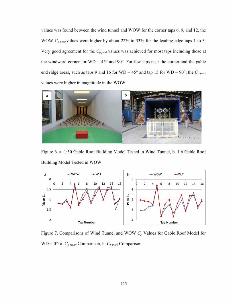
125

values was found between the wind tunnel and WOW for the corner taps 6, 9, and 12, the

WOW Cp peak values were higher by about 22% to 33% for the leading edge taps 1 to 3.

Very good agreement for the Cp peak values was achieved for most taps including those at

the windward corner for WD = 45° and 90°. For few taps near the corner and the gable

end ridge areas, such as taps 9 and 16 for WD = 45° and tap 15 for WD = 90°, the Cp peak

values were higher in magnitude in the WOW.

Figure 6. a. 1:50 Gable Roof Building Model Tested in Wind Tunnel, b. 1:6 Gable Roof

Building Model Tested in WOW

Figure 7. Comparisons of Wind Tunnel and WOW Cp Values for Gable Roof Model for

WD = 0°: a. Cp mean Comparison, b. Cp peak Comparison

a b

a b

126





5.4.2.2 Pressure Coefficient Comparisons of Hip Roof Building

Figure 10 shows the 3:12 hip roof building models tested in the wind tunnel and

WOW, respectively. Figures 11 to 13 show the comparative results of Cp mean and Cp peak

for WD = 0°, 45°, and 90°. For all WDs, the trends of the Cp mean and Cp peak obtained in

the two facilities compared well. For WD = 0°, there was very good agreement between

the two facilities, except that the WOW estimates for Cp peak values for windward leading

edge taps 1 and 2 were about 10% higher in magnitude compared to the wind tunnel val-

a b

a b

127

ues. This was similar to the gable roof case for which WOW produced higher peak pres-

sure coefficients for the leading edge taps. For WD = 45°, most of the values were in

agreement except for taps 4, 12, and 14. The highest percentage difference was obtained

for tap 12 located at the windward corner near the sloped ridge for which the Cp peak val-

ues were -5.0 and -6.5 for the wind tunnel and WOW, respectively. This indicates that the

peak suction coefficient in WOW was 23% higher than the wind tunnel value. For the

WD = 90°, the Cp mean values matched well between the two facilities while the Cp peak

values matched better for the taps subjected to stronger suctions such as taps 12 and 13

near the windward corner of the sloped ridge. A difference of about 14% was obtained

for tap 14 in which case the wind tunnel estimated value was higher in magnitude.

Figure 10. a. 1:50 Hip Roof Building Model Tested in Wind Tunnel, b. 1:6 Hip Roof

Building Model Tested in WOW

b a

128

Figure 11. Comparison of Wind Tunnel and WOW Cp Values for Hip Roof Model for






a b

a b

a b

129

5.4.2.3 Summary of Wind Tunnel and WOW Results Comparison

Pressure coefficients obtained using the two facilities were in reasonable agree-

ment for most cases where high suctions were experinenced. This validated the efficacy

of partial turbulnece flow simulation to induce realistic mean and peak pressures on low-

rise buildings with dimensions not exceeding those of typical residential homes. For

some critical locations, where roofing components are often damaged due to high suc-

tions during windstorms, such as the roof leading edge (for WD = 0°), gable end ridge

(for WD = 45°), and windward corner near sloped hip (for WD = 45°), the WOW esti-

mated peak pressure coefficients were higher in magnitude than their wind tunnel coun-

terparts. In the literature it was hypothesized that some of these differences can be due to

Reynolds number (Re) effect, as suggested for Silsoe Building by Hoxey et al. (1998) and

Texas Tech Building by Cheung et al. (1997). Additional research will be performed in

future to closely investigate Re effects by testing models under a wide range of wind

speeds in the WOW.

5.5 Discontinuous Perforated Parapets for Mitigating Roof Negative Pressures

5.5.1 Test Models

After validating the partial turbulence flow simulation methodology for testing

large-scale models, WOW experimentation was performed to study the effectiveness of

discontinuous perforated parapets in alleviating high suctions (in magnitude) at critical

locations on the roof of low-rise buildings. The 1:6 large-scale models of the two story

gable and hip buildings with 3:12 roof slope were tested with and without parapets. The

large scale modeling allowed accurate fabrication and installation of 33% porous discon-

tinuous parapets. For the gable roof building model the parapets were installed close to

130

four roof corners and also at the two gable end ridge intersections (see Fig. 14). For the

hip roof building model the parapets were installed close to four roof corners near the

sloped ridge and eave intersections (see Fig. 15). The length of each parapet was 15.2 cm,

that is, 10% of the shorter horizontal dimension of the test building as was proposed by

Suaris and Irwin (2010). The height of the parapet was 3.8 cm, thus its ratio to the roof

eave height of the building was about hp/Heave = 0.034. In this study, a shorter parapet

height ratio was used than those used in past studies. This was done to facilitate installa-

tion and lower the cost of construction of parapets on prototype buildings. All the tests

were conducted in the 12-Fan WOW facility using the partial turbulence simulation tech-

nique. Each building model was tested for seven wind directions -- WD = 0° to 90°, with

15° increments. The duration of each test was 3 min and pressure data collection method

was similar to that described in Section 5.4.2.

Figure 14. Discontinuous Perforated Parapets Installed on Gable Roof Building Model

131

Figure 15. Discontinuous Perforated Parapets Installed on Hip Roof Building Model

5.5.2 Results for Gable Roof Building Model

Figures 16 to 22 show the comparisons of mean (Cp mean) and peak (Cp peak) pres-

sure coefficients without and with the discontinuous perforated parapets for the gable

roof model. The results show the efficacy of the parapets in significantly reducing the

uplift pressures near the roof corners and gable end ridge intersections. The highest re-

ductions in Cp mean values were noted for gable end ridge tap 15 for WD = 0° (~33% re-

duction, see Fig. 16a) and roof corner tap 13 for WD = 60° (~60% reduction, see Fig.

20a). The highest reductions in Cp peak values were noted for several taps at critical loca-

tions with high suctions, for example, edge tap 6 for WD = 15° (~40%, see Fig. 16b), ga-

ble end ridge tap 16 for WD = 45° (~72% reduction, see Fig. 19b), and corner tap 13 for

WD = 60° (~55% reduction, see Fig. 20b). In the work performed by Suaris and Irwin

(2010), the highest reduction in peak pressure coefficients was about 60% while using

perforated parapets of similar configurations as used in this study.

132

The reductions in area-averaged peak pressure coefficients were estimated for Ar-

ea 1 (corner area with taps 6 to 14) and Area 2 (gable end ridge intersection area with

taps 15 and 16) (see Fig. 14 for Area 1 and Area 2). Significant reductions in area aver-

aged peak pressures were obtained, e.g.: 20% reduction for Area 1 for WD = 45°; 48%

and 31% reductions for Area 2 for WD = 45° and 90°, respectively. Figure 23 compares

the without- and with-parapet cases by showing the instantaneous pressure coefficient

surfaces for Area 1 for WD = 45° for the instant of time when the peak area-average up-

lift pressure attained the highest magnitude in each case. In Fig. 23, three-dimensional

contours are plotted to visualize the spatial distributions of recorded instantaneous pres-

sure coefficients of 9 taps close to roof corner region (Area 1) without- and with- parapet

cases for WD = 45°. The contours show instantaneous pressure coefficients 𝐶𝐶 = ( )

corresponding to time t when the area-averaged peak pressure coefficient reached the

highest magnitude (largest suctions occurred at t = 90.3 s and 31.0 s for without- and

with-parapet cases, respectively). The without-parapet contour (Fig. 23b) shows that the

worst uplift pressures occurred at taps 13 and 14 located close to the roof edge in a region

susceptible to strong conical vortices generated for cornering winds at WD = 45°. Signif-

icant reductions of suction pressures were observed on taps 13 and 14 after the discontin-

uous perforated parapets were installed (see Fig. 23c). The overall results demonstrated

that the extreme uplift pressures were alleviated by installing discontinuous perforated

parapets near critical roof locations where damage initiation commonly occurs during

severe windstorms. The discontinuous parapets had minimal effects on pressures on roof

areas farther away from the corners and ridges. Results showed that the parapets did not

133

have any unwanted effect (such as increase in uplift magnitude) at the center taps (i.e.

taps 1-5). For comparison purposes limited tests were also performed in the wind tunnel

with and without the porous parapets. Figures 23d and 23e show the contours obtained

from wind tunnel for Area 1 and a 20% reduction was observed which is same as the

WOW result. However, for Area 2 the reductions were 25% and 10% for WD = 45° and

90°, respectively. These reductions estimated in the wind tunnel were lower than the re-

ductions estimated in the WOW testing which were 48% and 31% for WD = 45° and 90°,

respectively.

Figure 16. Comparisons of Cp Values Without and With Parapets on Gable Roof Model

for WD = 0°: a. Cp mean Comparison, b. Cp peak Comparison


for WD = 15°:, a. Cp mean Comparison, b. Cp peak Comparison

a b

a b

134






for WD =60°: a. Cp mean Comparison, b. Cp peak Comparison

a b

a b

a b

135





a b

a b

a

136

Figure 23. Comparison of Instantaneous 3-D Pressure Coefficient Contours Without and

With Parapets for Gable Roof Corner (Area 1) for WD = 45°: a. Tap Locations for Area 1

(Prototype Dimension), b. Pressure Coefficient Contours Without Parapets for WOW, c.

Pressure Coefficient Contours With Parapets for WOW, d. Pressure Coefficient Contours

Without Parapets for Wind Tunnel, e. Pressure Coefficient Contours With Parapets for

Wind Tunnel.

5.5.3. Results for Hip Roof Building Model

Figures 24 to 30 show the comparisons of pressure coefficients without and with

the discontinuous parapets for the hip roof model. The parapets did not have significant

effects on Cp mean values. The highest reductions in Cp peak values were noted for corner

b c

d e

137

taps near the sloped ridge line, for example, 57% and 54% reductions for taps 12 and 13,

respectively, for WD = 45° (see Fig. 27b) and 54% reduction for tap 13 for WD = 60°

(see Fig. 28b). The reduction in area averaged peak pressure coefficient was estimated for

corner Area 1. Similar to the gable roof case, the highest reduction (38%) was achieved

for diagonal wind direction WD = 45°. In Fig. 31, three-dimensional pressure coefficient

contours are plotted for Area 1 for WD = 45°. The contours correspond to the time when

the area-averaged suction reached the highest magnitude (largest suctions occurred at t =

16.8 sec and t = 62.9 sec for without- and with- parapet case, respectively). The without-

parapet contour (Fig. 31b) shows that the large suctions occurred at taps 12 and 13 near

the corner and the suctions were significantly mitigated after installing the perforated

parapets (Fig. 31c). Thus the parapets were effective in alleviating high suctions for cor-

ner zones on both sides of the sloped ridge line where damage initiation often occurs.

About 18% reduction was estimated by analyzing the wind tunnel results (Figs. 31d and

31e), which was lower than the 38% reduction obtained in the WOW. The differences

could due to Reynolds number effects as the Reynolds number in WOW was about 15

times greater than that in the wind tunnel.

Figure 24. Comparisons of Cp Values Without and With Parapets on Hip Roof Model for


b a

138







b a

b a

b a

139







b a

b a

b a

140

Figure 31. Comparison of Instantaneous 3-D Pressure Coefficient Contours Without and

With Parapets for Hip Roof Corner (Area 1) for WD = 45°: a. Tap Locations for Area 1

c b

a

d e

141

(Prototype Dimension), b. Pressure Coefficient Contours Without Parapets for WOW, c.

Pressure Coefficient Contours With Parapets for WOW, d. Pressure Coefficient Contours

Without Parapets for Wind Tunnel, e. Pressure Coefficient Contours With Parapets for

Wind Tunnel.

5.6 Summary and Conclusions

A methodology was presented for testing large-scale models of low-rise buildings

in flows that replicate only the high frequency fluctuations of the longitudinal wind ve-

locity. Flow management devices were used in an open-jet 12-fan WOW facility to gen-

erate a turbulence spectrum with high frequency turbulence components similar to those

of ABL flows. It was hypothesized that two flows – characterized, respectively, by a full

turbulence spectrum (achieved in an ABL wind tunnel flow) and by a partial turbulence

spectrum with missing low frequency fluctuations (achieved in the WOW flow) – will

induce similar wind effects (e.g., pressure coefficients) if both flows have (1) similar high

frequency content, and (2) the mean wind speed U in the flow with weak low frequency

fluctuations is augmented by an increment ΔU to compensate for the missing fluctua-

tions. A numerical iteration procedure, developed for estimating ΔU, was shown to yield

good agreement of the high frequency portions of the prototype counterparts of the partial

spectrum obtained in the WOW on the one hand and the ABL wind tunnel full spectrum

on the other. The hypothesis was validated by comparing pressures measured on 3:12 ga-

ble and hip roof building models tested in a full turbulence spectrum flow in the ABL

wind tunnel and a partial turbulence spectrum flow in the WOW. Mean and peak pressure

coefficients obtained in the two facilities were in reasonable agreement for most cases.

For some tap locations in high suction zones on the roof, the WOW estimated peak pres-

142

sure coefficients were higher in magnitude than their wind tunnel counterparts. Further

research will be conducted to evaluate if these differences are due to Reynolds number

effects and/or slightly higher spectral content in the WOW. After validating the partial

turbulence flow simulation methodology for testing large-scale models, WOW experi-

mentation was performed to study the effectiveness of discontinuous perforated parapets

in alleviating high suction pressure at critical roof locations. For the gable roof, a maxi-

mum reduction of 72% in peak pressure coefficient was observed for a gable end ridge

tap when using the parapet (a maximum reduction of 60% was observed in a wind tunnel

study by Suaris and Irwin (2010) while using similar perforated parapets on a 3:12 gable

roof). For the hip roof, a maximum reduction of 57% was observed for a corner tap near

the sloped ridge line. Significant reductions in area averaged peak pressures for high suc-

tion zones were obtained for both roofs when using discontinuous parapets (up to 48%

and 38% for gable and hip roofs, respectively). Overall, the discontinuous porous para-

pets, which can be also used as architectural features, performed well in reducing high

suctions at critical roof locations and did not have any unwanted effect on the remaining

roof area. These simple architectural features can be retrofitted in existing buildings or

constructed on new low-rise buildings to improve roof performance. Limited compari-

sons showed that the percentage reductions in area-averaged pressures were in most cases

higher in the WOW large-scale testing than those obtained in the wind tunnel small-scale

testing. This study demonstrated that the partial simulation methodology can be effective

in validating mitigation techniques to reduce wind damage on low-rise buildings. Such

simulations with deficient low-frequency spectral content are freed of integral length

scale constraints so that model length scales are only limited by blockage considerations.

143

This is a major advantage, because it allows for both testing at higher Reynolds number

and better spatial resolution of the pressure taps in high pressure zones.


We acknowledge the National Science Foundation (NSF) Award No. CMMI-

1151003 for supporting the 12-fan Wall of Wind (WOW) research. WOW instrumenta-

tion has been supported through the NSF MRI Award No. CMMI-0923365. Dr. Emil

Simiu partly contributed to Section 3.1 and provided helpful comments on this work.

WOW facility construction was supported by the Florida Center of Excellence in Hurri-

cane Damage Mitigation and Product Development, Department of Energy, Renaissance

Re, Roofing Alliance for Progress, and AIR Worldwide. We also express our apprecia-

tion to RWDI USA LLC for their great support in performing the tests for this study. The

findings presented in this paper, however, are those of the authors alone and do not nec-

essarily represent the views of sponsoring agencies.

5.8 Reference

ASCE. (2010). “Minimum design loads for buildings and other structures.” ASCE/SEI 7-10, Reston, VA.

ASCE. (2012). “Wind tunnel testing for buildings and other structures.” ASCE/SEI 49-12, Reston, VA.

Aly, A. M., Bitsuamlak, G. T., and Gan Chowdhury, A. (2012). “Full-scale aerodynamic testing of a loose concrete roof paver system.” J. Eng. Struct., 44, 260-270.

Aly, A. M., Gan Chowdhury, A., and Bitsuamlak, G. (2011). “Wind Profile Management and Blockage Assessment of a New 12-Fan Wall of Wind Facility at FIU.” J. Wind Struct., 14(4), 285-300.

Banks D. (2011). “Measuring peak wind loads on solar power assemblies.” The 13th In-ternational Conference on Wind Engineering, Amsterdam, Netherlands.

Baskaran A., and Stathopoulos, T. (1998). “Roof corner pressure loads and parapet con-figurations.” J. Wind Eng. Ind. Aerodyn., 29, 79-88.

144

Bitsuamlak, G.T., Gan Chowdhury, A., and Sambare, D. (2009). “Application of a full-scale testing facility for assessing wind-driven-rain intrusion.” J. Building Environm., 44(12), 2430-2441.

Bitsuamlak, G. T., Warsido, W., Ledesma E., and Gan Chowdhury, A. (2013). “Aerody-namic Mitigation of Roof and Wall Corner Suctions Using Simple Architectural Ele-ments.” J. Eng. Mech., 139, 396-408.

Blessing, C., Gan Chowdhury, A., Lin, J., and Huang, P. (2009). “Full-scale validation of vortex suppression techniques for mitigation of roof uplift.” J. Eng. Struct., 31(12), 2936–2946.

Cheung, J. C. K., Holmes, J. D., Melbourne, W. H., Lakshmanan, N., and Bowditch, P. (1997). “Pressure on a 1:10 scale model of the Texas Tech Building.” J. Wind Eng. Ind. Aerodyn., 69-71, 529-538.

Cochran, J. S. and English, E. (1997), “Reduction of roof wind loads by architectural fea-tures”, Architectural Science Review, 40, 79-87.

Fu, T.C., Aly, A. M., Gan Chowdhury, A., Bitsuamlak, G., Yeo, D., and Simiu, E. (2012). “A proposed technique for determining aerodynamic pressure on residential homes.” J. Wind Struct., 15(1), 27.-41

Huang, P., Gan Chowdhury, A., Bitsuamlak, G., and Liu, R. (2009). “Development of devices and methods for simulation of hurricane winds in a full-scale testing facility.” J. Wind Struct., 12(2), 151-177.

Holmes, J.D. (2007). Wind Loading of Structures, 2nd Ed. Taylor & Francis, London.

Hoxey, R. P., Reynolds, A. M., Richardson, G. M., Robertson, A. P., and Short, J. L. (1998). “Observations of Reynolds number sensitivity in the separated flow region on a bluff body.” J. Wind Eng. Ind. Aerodyn., 73, 231-249.

Irwin, P. (1981). “The design of spires for wind simulation.” J. Wind Eng. Ind. Aerodyn., 7, 361-366.

Irwin, P. (2009). “Wind engineering research needs, building codes and project specific studies.” 11th Americas Conference on Wind Engineering, San Juan, Puerto Rico.

Irwin, P., Cooper, K., and Girard, R. (1979). “Correction of distortion effects caused by tubing systems in measurements of fluctuating pressures.” J. Wind Eng. Ind. Aero-dyn., 5, 93-107.

Jones, N.P., Reed, D.A., and Cermak, J.E. (1995). “National wind-hazards reduction pro-gram.” J. Prof. Issues Eng. Educ. Pract., 121(1), 41–46.

Kopp, G. A., and Banks, D. (2013). “Use of the wind tunnel test method for obtaining

145

design wind loads on roof-mounted solar arrays.” J. Struct. Eng., 139, 284-287.

Kopp, G.A., Mans, C., and Surry, D. (2005). “Wind effects of parapets on low buildings: Part 4. Mitigation of corner loads with alternative geometry.” J. Wind Eng. Ind. Aero-dyn., 93, 873-888.

Kopp, G. A., Morrison, M. J., Gavanski, E., Henderson, D. J., and Hong, H. P. (2010). “The ‘Three Little Pigs’ project: hurricane risk mitigation by integrated wind tunnel and fullscale laboratory tests.” Nat. Haz. Rev., 11, 151–161.

Lin, J.X., and Surry, D. (1993). “Suppressing extreme suction on low buildings by modi-fying the roof corner geometry.” Proc. 7th US National Conf. on Wind Eng., Univ. of Calif., USA, Session 3A.

Liu, Z., Brown, T.M., Cope, A.D., and Reinhold, T.A. (2011). “Commissioning of the wind test capabilities of the IBHS Research Center.” Proc. 13th Int. Conf. Wind Eng., Amsterdam, Netherlands.

MDC-BCCO. Post hurricane Wilma progress assessment. Miami-Dade County Building Code Compliance Office, Miami, FL, 2006:1-22.

Melbourne W. H. (1980). “Turbulence effects on maximum surface pressures – a mecha-nism and possibility of reduction.” J. Wind Eng., 1, 521-551.

Mensah A. F., Datin, P. L., Prevatt, D., Gupta, R., and van de Lindt, J. W. (2011). “Data-base-assisted design methodology to predict wind – induced structural behavior of a light-framed wood building.” J. Eng. Struct., 33, 674-684.

Natarajan, D., and Hangan, H. (2010). “Preliminary numerical simulation of axi-symmetric flows in WindEEE dome facility.” Proc. 5th Int. Symp. on Computational Wind Engineering (CWE2010), International Association for Wind Engineering (IAWE), Kanagawa, Japan.

National Oceanic and Atmospheric Administration (2013). Population trends from 1970 to 2020. National Costal Population Report.

Richards, P.J., Hoxey, R.P., Connell, R.P., and Lander, D.P. (2007). “Wind-tunnel mod-elling of the Silsoe Cube.” J. Wind Eng. Ind. Aerod., 95, 1384-1399.

Sadek, F., and Simiu, E. (2002). “Peak non-Gaussian wind effects for database-assisted low-rise building design.” J. Eng. Mech., 128(5), 530-539.

Simiu, E. (2011), Design of Buildings for Wind¸ Wiley, Hoboken.

Simiu, E., Bitsuamlak, G., Gan Chowdhury, A., Li, R., Tecle, A., and Yeo, D.H. (2011). “Testing of residential homes under wind loads.” J. Nat. Hazards Rev., 12(4), 166-170.

146

Simiu, E. and Scanlan, R.H. (1996). Wind Effects on Structures, Wiley, New York

Stathopoulos, T., Marathe, R., and Wu, H. (1999). “Mean wind pressure on flat roof cor-ners affected by parapets: field and wind tunnel studies.” J. Eng. Struct., 21, 629-638.

Suaris, W., and Irwin, P. (2010). “Effect of roof-edge parapets on mitigating extreme roof suctions.” J. Wind Eng. Ind. Aerodyn., 98, 483–491.

Suresh, Kumar, K., and Stathopoulos, T. (1998), “Power spectra of wind pressures on low building roofs”, J. Wind Eng. Ind. Aerodyn., 74-76, 665-674.

Surry D. and Lin, X. J. (1995). “The effect of surroundings and roof corner geometric modifications on roof pressures on low-rise buildings.” J. Wind Eng. Ind. Aerodyn., 58, 113-138.

Tecle, A., Bitsuamlak, G., Suksawang N., Gan Chowdhury, A., and Fuez, S. (2013). “Ridge and field tile aerodynamics for a low-rise building: a full-scale study.” Wind and Struct., 16(4), 301-322.

Tieleman, H. W. (2003). “Wind tunnel simulation of wind loading on low-rise structures: a review.” J. Wind Eng. Ind. Aerod., 91, 1627-1649.

Tieleman, H. W., Hajj, M. R., and Reinhold, T. A. (1998). “Wind tunnel simulation re-quirements to asses wind loads on low-rise buildings.” J. Wind Eng. Ind. Aerod., 74-76, 675-685.

Yamada, H., and Katsuchi, H. (2008). “Wind-tunnel study on effects of small-scale tur-bulence on flow patterns around rectangular cylinder.” Proc. of the 4th International Colloquium on Bluff Bodies Aerodynamics & Applications, Italy.

Yeo, D., and Gan Chowdhury, A. (2013). “A simplified wind flow model for the estima-tion of aerodynamic effects on small structures.” J. Eng. Mech., 139, 367-375.

147

CHAPTER VI

SUMMARY AND CONCLUSION

148

CHAPTER VI

SUMMARY AND CONCLUSION

This chapter summarizes the conclusions of this dissertation. The achievements in

this dissertation are summarized into 3 parts: 1. A partial turbulence simulation method-

ology using an iterative procedure was successfully developed to yield good agreement of

the high frequency portion with the ABL flow. 2. Pressure results obtained using large-

scale models at the WOW facility compared well to both the full-scale TTU and Silsoe

building and small-scale wind tunnel model measurements. This validated the partial tur-

bulence simulation methodology. 3. The effectiveness of discontinuous perforated para-

pets in alleviating high suction pressure at critical roof locations was demonstrated by

testing typical two-story residential buildings in the WOW using the partial turbulence

simulation method. The details are described in the following sections.

6.1 Flow simulation

A partial turbulence simulation methodology using an iterative procedure was de-

veloped. The simulation was shown to be appropriate for testing of large-scale models in

aerodynamic facilities. Such simulation with deficient low-frequency spectral content is

freed of integral length scale constraints so that model length scales are only limited by

blockage considerations. This is a major advantage, because it allows for both testing at

higher Reynolds number and greater spatial resolution of the pressure taps in high pres-

sure zones. The methodology was applied successfully in the 12-fan WOW open-jet wind

testing facility and partial simulation results were obtained. Flow management devices

were used in an open-jet 12-fan WOW facility to generate turbulence spectrum with high

frequency components similar to those of ABL flows. A methodology was presented for

149

testing large-scale models of low-rise buildings in flows that replicate only the high fre-

quency fluctuations of the longitudinal wind velocity. It was hypothesized that two flows

– characterized, respectively, by a full turbulence spectrum (achieved in an ABL wind

tunnel flow) and by a partial turbulence spectrum with missing low frequency fluctua-

tions (achieved in the WOW flow) – will induce similar wind effects if both flows have

(1) similar high frequency content, and (2) mean wind speed in the flow with weak low

frequency fluctuations is augmented by an increment to compensate for the missing fluc-

tuations. A numerical iteration procedure was shown to yield good agreement of the high

frequency portion of the partial spectrum obtained in the laboratory on the one hand and

the ABL spectrum model on the other. The high frequency portion of the partial spectrum

obtained in the WOW compared well with the full spectrum in an ABL wind tunnel and

prototype full spectrum for the TTU and Silsoe site.

6.2 Pressure validation

Pressure measurements and comparisons of mean and peak pressure coefficient

estimates were performed for (1) the partial turbulence flow in small and large-scale 12-

Fan WOW, and (2) the full turbulence flow in the ABL wind tunnel and field data for

TTU and Silsoe sites. For four gable and hip roof low rise building models it was shown

that both the wind tunnel and the small-scale WOW produced comparable high suctions

(high peak pressure coefficients) for critical locations near the leading edge for low-slope

roof, leeward edge, gable end ridge, and downwind of sloped hips. The results showed

that similar high suction can occur near the gable end ridge for cornering wind and the

downwind side of the sloped hip for both cornering wind and wind perpendicular to the

eave. The findings provide an explanation to why failures initiate mostly at these ridge

150

and hip locations. Besides using small-scale WOW to validate the pressure field, the

large-scale 12-Fan WOW was also used to perform and verify the effectiveness of partial

turbulence simulation by comparing the WOW pressure coefficients with their full-scale

(TTU and Silsoe buildings) and smaller model-scale (wind tunnel) counterparts. For the

open terrain, 1:6 TTU building model and 1:5 Silsoe building model were tested and the

pressure coefficients were compared with their benchmark prototype counterpart. For

most cases, the pressure results obtained from WOW partial simulation for taps experi-

encing high mean and peak suctions were in reasonable agreement with their full-scale

counterparts. For the suburban terrain, 3:12 gable and hip roof building models were test-

ed and the pressure coefficients were compared with those obtained in full turbulence

spectrum flow in an ABL wind tunnel. The mean and peak pressure coefficients obtained

in the two facilities were in reasonable agreement for most cases. All the pressure com-

parisons showed that the partial turbulence simulation approach was effective aerody-

namically.

6.3 Uplift pressure mitigation

WOW experimentation was performed to study the effectiveness of discontinuous

perforated parapets in alleviating high suction pressure at critical roof locations. For the

3:12 gable roof, a maximum reduction of 72% in peak pressure coefficient was observed

for a gable end ridge tap when using the parapet. For the 3:12 hip roof, a maximum re-

duction of 58% was observed for a corner tap near the sloped ridge line. Significant re-

ductions in area averaged peak pressures for high suction zones were obtained for both

roofs when using discontinuous parapets (up to 48% and 38% for gable and hip roofs,

respectively). Overall, the discontinuous porous parapets, which can be also used as ar-

151

chitectural features, performed well in reducing high suctions at critical roof locations.

These simple architectural features can be retrofitted in existing buildings or constructed

on new low-rise buildings to improve roof performance. Limited comparisons showed

that the percentage reductions in area-averaged pressures using the discontinuous porous

parapets were in most cases higher in the WOW large-scale testing than those obtained in

the wind tunnel small-scale testing. In addition, the experiments performed for testing the

effects on parapets showed that the partial simulation methodology can be effective in

validating mitigation techniques to reduce wind damage to low-rise buildings.

152

CHAPTER VII

RECOMMENDATIONS FOR FUTURE RESEARCH

153

CHAPTER VII

RECOMMENDATIONS FOR FUTURE RESEARCH

Future tests should be planned to refine the partial turbulence simulation tech-

nique and validate it for a wide range of model-to-full-scale ratios. These tests should ad-

dress the effects of Reynolds Number (Re), the effects of sudden change of internal pres-

sure, and the effects of no-stationary gusts.

7.1 Reynolds number

Hoxey (1998) described that bluff body aerodynamic effects can be highly de-

pended on Reynolds Number (Re). In 2001, Schewe also carried out a series of tests and

discovered that Re had significant effects on the mean pressure coefficients (Cp) for the

structures with sharp edges. The Re number in Schewe’s study ranged between 104 and

107. In general, the Re values of conventional wind tunnel tests and WOW tests are

about 104 and 106, respectively. It is necessary to further investigate Re effects on civil

engineering structures. Moreover, different from the global Re mentioned above, the ef-

fects of local Re could be also important. These Re effects are due to the local aerody-

namic loads generated by architectural details. In most cases, the testing of buildings in

small-scale experimentation is usually simplified. However, architectural features are im-

portant in terms of local aerodynamic loads. Thus there is a need to perform partial turbu-

lence simulation experiments using large-scale testing models to find local Re effects.

7.2 Internal pressure

The net wind pressures acting on building envelopes are the combination of ex-

ternal and internal pressures. The opening sizes and locations are the most important fac-

tors influencing internal pressures. During hurricanes wind-borne debris may create a siz-

154

able opening suddenly and result in abrupt change of the internal pressure. There is a

need to study the effect of partial simulation flows on internal pressures due to sudden

breach of envelope.

7.3 Non-Stationary gusts and rapid directionality changes

During extreme events such as hurricane, strong wind gust and rapid directionali-

ty changes may occur. Such transient effects may have significant influence on wind

loading which can exceed quasi-steady loading. Partial turbulence simulation methodolo-

gy can be used to perform research on non-stationary phenomena and their effects on

structures.

155

VITA

EDUCATION 2007-Present Doctoral Candidate,

Department of Civil and Environmental Engineering, Florida International University, Miami, FL.

2004 M.S., Department of Civil and Environmental Engineering, West Virginia University, Morgantown, WV.

2000 B.E., Department of Civil and Environmental Engineering, National Central University, Taoyuan, Taiwan

PROFESSIONAL EXPERIENCE 2008-2013 Research Assistant, International Hurricane Research Center,

Florida International University, Miami, FL. 2007-2008 Teaching Assistant, Department of Civil and Environmental Engineering,

Florida International University, Miami, FL. PUBLICATIONS AND PRESENTATIONS Fu, T.C., Aly, A.M., Bitsuamlak, G., Gan Chowdhury, A., Simiu, E. (2010) “Flow Simu-lation in 12-Fan Wall of Wind Testing Facility” The 2nd American Association for Wind Engineering Workshop (2AAWE), Marco Island, Florida, USA, August 18-20, 2010. Fu, T.C., Aly, A.M., Gan Chowdhury, A., Bitsuamlak, G., Yeo, D.H. and Simiu, E. (2011), “Simplified wind flow and aerodynamic response of residential homes: Laborato-ry and Computational Fluid Dynamics simulations,” 4 International Conference on Ex-perimental Vibration Analysis for Civil Engineering Structures (EVACES 2011), Varen-na, Italy, October 3-5, 2011. Fu, T.C., Aly, A. M., Gan Chowdhury, A., Bitsuamlak, G., Yeo, D., and Simiu, E. (2012), “A Proposed Technique for Determining Aerodynamic Pressure on Residential Homes”, Wind and Structures, 15(1), 27-41. Fu, T.C., Gan Chowdhury, A., Bitsuamlak, G., Li, R. and Aly, A.M., (2011), “Wall of wind facility: low-rise buildings roof pressure validation,” The EMI 2011 Engineering Mechanics Institute Conference, Northeastern University, Boston, MA, USA, June 2-4, 2011. Fu, T.C, Gan Chowdhury, A., and Bitsuamlak, G., (2012) “An Open-Jet Test Facility Validation Using Comparison of Pressure Field on Buildings”, ASCE Advances in Hurri-cane Engineering Conference (ATC & SEC), Miami, United States, October 24-26, 2012.

156

Fu, T.C., Gan Chowdhury, A., Bitsuamlak G., Simiu, E. “Pressure Validation for an Open-Jet Wind Testing Facility”, submitted to Wind and Structures, Jul. 2013, in pro-gress. Fu, T.C., Gan Chowdhury, A., Smith D., Zisis I., Irwin P., Simiu E. “Experimental Simu-lation of Wind Pressures on Large-Scale Building Models and Comparisons with Field Measurements’, submitted to Journal of Wind Engineering and Industrial Aerodynamics, Sep. 2013, in progress. Fu, T.C., Gan Chowdhury, A., Zisis I., Irwin P., “Experimental Simulation of Wind Pres-sures on Large-Scale Building Models and Comparisons with Field Measurements’, submitted to Engineering Structures, Nov. 2103, in progress. Gan Chowdhury, A., Bitsuamlak, G., Fu, T., and Kawade, P. (2011), ”Study on Roof Vents Subjected to Simulated Hurricane Effects.” ASCE, Nat. Hazards Rev. 12, SPE-CIAL ISSUE: Hurricanes and Insurance, 158–165. TRAINING/PROFESSIONAL MEMBERSHIPS 2011-Present Membership of Chi-Epsilon Honor Society of Civil Engineering

Honor Society

Documents

Development of Effective Approaches to the Large-Scale