Development of an Active-Learning Lesson that Targets

The University of MaineDigitalCommons@UMaine

Electronic Theses and Dissertations Fogler Library

5-2017

Development of an Active-Learning Lesson thatTargets Student Understanding of PopulationGrowth in EcologyElizabeth [email protected]

Follow this and additional works at: http://digitalcommons.library.umaine.edu/etd

Part of the Biology Commons, and the Science and Mathematics Education Commons

This Open-Access Thesis is brought to you for free and open access by DigitalCommons@UMaine. It has been accepted for inclusion in ElectronicTheses and Dissertations by an authorized administrator of DigitalCommons@UMaine.

Recommended CitationTrenckmann, Elizabeth, "Development of an Active-Learning Lesson that Targets Student Understanding of Population Growth inEcology" (2017). Electronic Theses and Dissertations. 2665.http://digitalcommons.library.umaine.edu/etd/2665

http://digitalcommons.library.umaine.edu?utm_source=digitalcommons.library.umaine.edu%2Fetd%2F2665&utm_medium=PDF&utm_campaign=PDFCoverPages

http://digitalcommons.library.umaine.edu/etd?utm_source=digitalcommons.library.umaine.edu%2Fetd%2F2665&utm_medium=PDF&utm_campaign=PDFCoverPages

http://digitalcommons.library.umaine.edu/fogler?utm_source=digitalcommons.library.umaine.edu%2Fetd%2F2665&utm_medium=PDF&utm_campaign=PDFCoverPages

http://digitalcommons.library.umaine.edu/etd?utm_source=digitalcommons.library.umaine.edu%2Fetd%2F2665&utm_medium=PDF&utm_campaign=PDFCoverPages

http://network.bepress.com/hgg/discipline/41?utm_source=digitalcommons.library.umaine.edu%2Fetd%2F2665&utm_medium=PDF&utm_campaign=PDFCoverPages

http://network.bepress.com/hgg/discipline/800?utm_source=digitalcommons.library.umaine.edu%2Fetd%2F2665&utm_medium=PDF&utm_campaign=PDFCoverPages

http://digitalcommons.library.umaine.edu/etd/2665?utm_source=digitalcommons.library.umaine.edu%2Fetd%2F2665&utm_medium=PDF&utm_campaign=PDFCoverPages

DEVELOPMENT OF AN ACTIVE-LEARNING LESSON THAT TARGETS STUDENT

UNDERSTANDING OF POPULATION GROWTH

IN ECOLOGY

By

Elizabeth Trenckmann

B.Sc. Maine Maritime Academy, 2015

A THESIS

Submitted in Partial Fulfillment of the

Requirements for the Degree of

Master of Science in Teaching

The Graduate School

The University of Maine

May 2017

Advisory Committee:

Michelle Smith, Associate Professor of the School of Biology and Ecology, Advisor

Mindi Summers, Instructor of Ecology and Evolutionary Biology

Sara Lindsay, Associate Professor of Marine Sciences

Karen Pelletreau, Lecturer in Biology Education

ii

© 2017 Elizabeth Trenckmann

All Rights Reserved

DEVELOPMENT OF AN ACTIVE-LEARNING LESSON THAT TARGETS STUDENT

UNDERSTANDING OF POPULATION GROWTH

IN ECOLOGY

By Elizabeth Trenckmann

Thesis Advisor: Dr. Michelle K. Smith

An Abstract of the Thesis Presented

in Partial Fulfillment of the Requirement for the

Degree of Master of Science in Teaching

May 2017

Integrating quantitative literacy skills into the undergraduate biology curriculum has been

advocated as a way to better reflect the tools and practices used by scientists. One area where students

often need and can develop quantitative skills is population ecology, and previous studies have shown

that students often have conceptual difficulties in this area. The focus of this thesis project was to explore

student thinking about population ecology and develop an in-class active-learning lesson that incorporates

quantitative skills for use in large-enrollment undergraduate biology courses. The development of this

lesson was guided by in depth reviews of literature, textbooks, and online teaching materials and data

gathered from assessment instruments. The lesson was designed using an iterative process involving

feedback from faculty and student learning data. The result of this process was a lesson that asks students

to “engage like scientists” as they make predictions, plot data, perform calculations, and interpret

information to investigate how ecologists measure and model population size. The final version of the

lesson was taught in three sections of a large enrollment undergraduate class at the University of Maine.

The impact of the lesson was assessed using formative and summative assessments including a pre/post-

test, clicker-based questions, and multiple-choice exam questions. Student performance increased

following peer discussion and on post-test questions. Students also performed well on end-of-unit exam

questions targeting similar concepts.

iii

ACKNOWLEDGEMENTS

First and foremost, I would like to thank Dr. Michelle Smith and Mindi Summers for

their constant support, feedback, and encouragement throughout this entire project. I am very

appreciative of the continuous communication, regular meetings, and guidance they provided me

with throughout this past year and a half. Equally helpful was the input and engagement from my

other committee members, Dr. Sara Lindsay and Dr. Karen Pelletreau. Furthermore, I would like

to thank Erin Vinson, Carrie Eaton, Ken Akiha, Justin Lewin, Emilie Brigham, and Gabrielle

Holt for their helpful feedback throughout this project.

I would also like to thank Dr. Farahad Dastoor for allowing the developed lesson to be

taught in his course, and would like to acknowledge the participation and contribution of all of

the students who actively engaged in this lesson and answered the pre/post questions. Many

others also contributed ideas and preliminary data to this project for which I am thankful. I

would like to recognize Dr. Amanda Klemmer for inviting me to pilot the first version of the

developed lesson in her course. The recommendations and suggestions of the University of

Maine School of Biology and Ecology Teaching and Learning Journal Club, Maine Center for

Research in STEM Education (RiSE Center), and the Ecology of Evolution and Everything

Seminar (EES) were invaluable to the development of this lesson. This material is based upon

work supported by the National Science Foundation grant 1322556.

iv

TABLE OF CONTENTS

ACKNOWLEDGEMENTS ........................................................................................................... iii

LIST OF TABLES ......................................................................................................................... ix

LIST OF FIGURES .........................................................................................................................x

Chapter

1. LITERATURE REVIEW ON THE IMPORTANCE OF ACTIVE LEARNING AND

STUDENT CONCEPTUAL DIFFICULTIES IN ECOLOGY .......................................................1

1.1 Overview ................................................................................................................................1

1.2 Active learning and its importance in the classroom .............................................................1

1.2.1 Inclusive teaching .......................................................................................................1

1.2.2 What is active learning? ..............................................................................................2

1.2.2.1 Questioning techniques ................................................................................2

1.2.2.2 Individual techniques ...................................................................................3

1.2.2.3 Cooperative learning techniques ..................................................................3

1.2.3 Benefits of active learning ..........................................................................................7

1.3 Persistent conceptual difficulties in ecology ..........................................................................9

1.3.1 Importance of ecology in undergraduate education ....................................................9

1.3.2 Literature review of student understanding of population growth ............................10

1.3.3 EcoEvo-MAPS assessment results ...........................................................................12

1.4 Purpose of this study ............................................................................................................13

v

2. ITERATIVE DEVELOPMENT OF AN ACTIVE-LEARNING BASED LESSON ................15

2.1 Overview ......................................................................................................................15

2.2 Background of population ecology .............................................................................15

2.2.1 Textbook review ..........................................................................................15

2.2.2 Review of available online materials ...........................................................17

2.3 Iterative lesson development .......................................................................................18

2.3.1 Developing population growth lesson with multiple

rounds of feedback .......................................................................................18

2.3.1.1 Lesson version 1: Intraspecific competition .................................23

2.3.1.2 Lesson version 2: Modeling and exploring population

size over time ...............................................................................25

2.3.1.3 Lesson version 3: Modeling and exploring population

size over time ...............................................................................26

2.3.1.4 Lesson version 4: Modeling and exploring how populations

change over time ...........................................................................27


change over time ..........................................................................29


grow over time .............................................................................30


grow over time .............................................................................32

vi

2.3.1.8 Lesson version 8: Describing and modeling populations

over time .....................................................................................33

2.3.1.9 Lesson version 9: Describing and modeling populations

over time ......................................................................................34

2.4 Recommendations for developing lessons ..................................................................34

2.4.1 Important steps and timeline for development .............................................35

3. AN ACTIVE-LEARNING LESSON THAT TARGETS STUDENT

UNDERSTANDING OF POPULATION GROWTH IN ECOLOGY ....................................40

3.1 Overview .....................................................................................................................40

3.2 CourseSource abstract ................................................................................................40

3.3 Scientific teaching context ..........................................................................................41

3.3.1 Learning goals ..............................................................................................41

3.3.2 Learning objectives ......................................................................................41

3.4 Introduction .................................................................................................................41

3.5 Lesson background information ..................................................................................43

3.5.1 Intended audience ........................................................................................43

3.5.2 Required learning time .................................................................................43

3.5.3 Pre-requisite student knowledge ..................................................................44

3.5.4 Pre-requisite teacher knowledge ..................................................................44

vii

3.6 Scientific teaching themes used in the lesson .............................................................45

3.6.1 Active learning ..............................................................................................45

3.6.2 Assessment ....................................................................................................45

3.6.3 Inclusive teaching .........................................................................................47

3.7 Lesson plan ..................................................................................................................47

3.7.1 Pre-class preparation .....................................................................................50

3.7.2 Think-Pair-Share and use of clickers ...........................................................51

3.7.3 Progressing through the lesson ....................................................................51

3.7.3.1 Introduction and assessing prior knowledge ..................................51

3.7.3.2 Quantifying population size ..........................................................53

3.7.3.3 Predicting and plotting population growth ...................................54

3.7.3.4 Identifying and comparing growth rate .........................................56

3.7.3.5 Determining the influence of carrying capacity ............................58

3.7.3.6 Synthesis .......................................................................................60

3.8 Teaching discussion ....................................................................................................61

3.8.1 Student performance and conceptual difficulties .........................................61

3.8.1.1 Pre/post multiple choice questions ................................................61

3.8.1.2 Exam questions .............................................................................66

3.8.1.3 Student perceptions .......................................................................67

3.9 Additional suggestions to enhance student learning while using this lesson ..............68

3.10 Conclusions ..............................................................................................................70

REFERENCES .............................................................................................................................71

viii

APPENDIX A: LESSON PRESENTATION SLIDES .................................................................77

APPENDIX B: RECOMMENDED INSTRUCTOR POPULATION

ECOLOGY RESOURCES ...........................................................................................................95

APPENDIX C: CLICKER QUESTIONS USED IN THE ACTIVITY AND

DISTRIBUTION OF STUDENT ANSWERS .............................................................................96

APPENDIX D: PRE/POST-TEST QUESTIONS AND DISTRIBUTION

OF STUDENT ANSWERS BEFORE AND AFTER INSTRUCTION .......................................97

APPENDIX E: EXAM QUESTIONS AND DISTRIBUTION OF STUDENT ANSWERS .....102

APPENDIX F: STUDENT WORKSHEET TO BE USED ALONG

WITH THE ACTIVITY. .............................................................................................................103

APPENDIX G: ATTITUDINAL QUESTIONS ASKED OF STUDENTS

AND DISTRIBUTION OF STUDENT RESPONSES ...............................................................105

BIOGRAPHY OF THE AUTHOR. .............................................................................................106

ix

LIST OF TABLES

Table 1.1: Conceptual difficulty topics in population ecology ..............................................11

Table 1.2: EcoEvo-MAPS identified conceptual difficulties ..................................................13

Table 2.1: Textbook review concepts .....................................................................................16

Table 2.2: Review of undergraduate lectures ..........................................................................17

Table 2.3: Summary of available resources in ecology education ..........................................19

Table 2.4: Summary of the learning objectives used in the lesson .........................................21

Table 2.5: Timeline for the development of a lesson .............................................................35

Table 3.1: Progression through the clicker based lesson .......................................................48

Table 3.2: Summary of assessment questions used in the lesson ..........................................62

Table 3.3: Student responses to attitudinal survey .................................................................68

Table B.1: Recommended instructor population ecology resources ......................................95

x

LIST OF FIGURES

Figure 2.1: Structure of the active-learning based lesson ........................................................22

Figure 2.2: Iterative design process of the lesson development ...............................................22

Figure 2.3: Suggested checklist for developing useful learning goals ....................................37

Figure 3.1: COPUS results from the lesson implementation ..................................................46

Figure 3.2: Pre/post assessment question responses ................................................................63

Figure 3.3: Student percent correct for exam questions ...........................................................67

1

CHAPTER 1

LITERATURE REVIEW ON THE IMPORTANCE OF ACTIVE LEARNING AND ON

STUDENT CONCEPTUAL DIFFICULTIES IN ECOLOGY

1.1 Overview

This thesis focuses on improving undergraduate student understanding of population

growth in ecology, increasing students’ quantitative reasoning skills, and developing classroom

activities and assessments that instructors can use in large-enrollment biology classes. Chapter 1

describes the background research conducted to develop a lesson that is inclusive, valuable, and

addresses important content areas where students have been shown to struggle.

1.2 Active learning and its importance in the classroom

1.2.1 Inclusive teaching

It is important that the pedagogical strategies employed in undergraduate classrooms

reflect an understanding of students’ needs and diverse backgrounds, learning styles, and abilities

(Ambrose et al., 2010). By implementing inclusive teaching strategies, instructors 1) provide

multiple opportunities for students to engage with and learn important content, 2) help students

connect with the course material in relevant and meaningful ways, and 3) allow students to feel

comfortable (Inclusive Teaching, 2016).

To implement inclusive teaching strategies in the classroom, instructors can use different

teaching approaches, activities, and assignments that can accommodate the needs of students and

provide flexibility in how students demonstrate content knowledge (Lage et al., 2000). For

2

example, by making content available through multiple mediums (e.g., on projected slides, on a

worksheet, verbally stated by peers/instructor) the instructor can optimize student success by

ensuring the students are receiving the information, regardless of how they best learn.

Additionally, by providing opportunities for both individual and group work to take place in the

classroom, the instructor allows students to learn in scenarios in which they are most

comfortable.

1.2.2 What is active learning?

Over the past decade, the focus of the university classroom has shifted away from the

traditional lecture based approach to a blend of pedagogical approaches that involve the student

in the learning process (Barr & Tagg, 1995). Inclusive teaching practices now include the use of

active-learning strategies such as asking students to answer questions and discuss their thinking

with classmates (Crouch and Mazur, 2001; Smith et al., 2009; Smith et al., 2011). Through this

student-centered approach the instructor can both increase student success and gain useful

information on student understanding (Singer et al., 2012). Such methods, which engage the

students in activities rather than passively listening to the instructor, are considered active

learning techniques (Faust and Paulson, 1998; Silberman, 1996). Below I discuss several

strategies regularly used in undergraduate classrooms to provide an idea of the diversity of active

learning techniques used by instructors.

1.2.2.1 Questioning techniques

An approach known as “questioning techniques” encourages the instructor to ask students

challenging questions that require the application of the concepts covered throughout the lecture

3

(Singer et al., 2012). For example, in a population ecology course the instructor can ask the

students to name abiotic and biotic factors that affect a population of barnacles. This method can

be employed to increase student involvement and interest in the classroom, even when lecture is

the primary content delivery method.

1.2.2.2 Individual techniques

Individual techniques, such as having students write a “one-minute paper” allow students

to be individually engaged in the learning process. This technique, originally reported by Angelo

and Cross (1993), helps instructors monitor student progress and provides students with a

consistent means of communicating with instructors. To implement, the instructor pauses class

during a lecture, poses a specific question, and provides time for the students to answer the

question in written format. Depending on the instructor’s objectives, this technique can be done

anonymously or with the student’s names attached.

1.2.2.3 Cooperative learning techniques

Cooperative learning is a subset of active learning that allows students to work together

in groups of three or more (Faust and Paulson, 1998). Groups work towards a common goal as

they complete tasks such as multiple step exercises, research projects, or presentations. Many

different types of cooperative learning techniques exist (examples 1-5):

1. Think-pair-share (TPS)- To implement TPS, the instructor poses a problem and

students think about the problem individually, work together to solve the problem, and

finally share their ideas with the entire class (Lyman, 1987; Kothiyal et al., 2013).

Through this model, students can individually think about the posed question, reflect on

4

their own thinking, and obtain immediate feedback from both the instructor as well as

their peers (Lyman, 1987).

2. Peer Instruction (PI)- Peer instruction is a cooperative learning technique that is closely

related to TPS (Lyman, 1992), but it is enhanced with the use of personal response

systems (clickers) which provide immediate assessment feedback (Duncan, 2006;

Knight and Wood, 2005; Smith et al., 2009). Clickers are remote control devices where

students typically respond to multiple choice questions, allowing the instructor to see

student responses in real-time. The use of clickers promotes anonymity, which can

reduce student discomfort in the classroom (Martyn, 2007). To use this instructional

technique the following steps can be used: 1) the instructor poses a thought-provoking

multiple choice question with multiple plausible incorrect answers, 2) students reflect

on the question, 3) students commit to an individual question, 4) the instructor reviews

student responses, 5) students discuss their thinking and answer choice with their

partners, and 6) the instructor reviews student responses and decides whether more

explanation is needed before moving onto the next concept (Mazur, 1997; Crouch and

Mazur, 2001).

Research indicates that the use of PI in the classroom increases conceptual understanding

in a variety of science, technology, engineering, and mathematics (STEM) courses (Crouch

and Mazur, 2001; Simkins and Maler, 2009; McConnell et al., 2006; Mora, 2010; Cortright

et al., 2005). In a study conducted by Crouch and Mazur (2001), student learning gains in a

traditional lecture and PI-based physics courses were compared by administering a

conceptual test, the Force Concept Inventory (FCI; Hestenes et al., 1992) to the students at

the beginning and end of each semester. The authors compared the results from PI classes to

5

10 years of historic data and found that the observed learning gains of students in the PI

instruction were twice as large as those observed in the traditional lecture (Crouch and

Mazur, 2001). Similarly, in a study conducted by McConnell et al. (2006), the average

differences between post and pre-test scores on the Geosciences Concepts Inventory (GCI;

Libarkin and Anderson, 2005) were greater in courses where PI was implemented.

The use of PI has also been shown to increase student understanding. For example, in a

study conducted to investigate how much students learned from peer discussion in a genetics

course, students answered paired sets of similar clicker questions throughout the semester

(Smith et al., 2009). Students were asked to answer one question individually (Q1), discuss

their thinking with their neighbors, and revote on the same question (Q1 after discussion).

Subsequent to this vote, the same students were asked a similar question (Q2) where no

discussion followed the individual vote. Results from this study indicate that most students

learned from the discussion of Q1, as the average percentage correct for Q2 was significantly

higher than for Q1 and Q1 after discussion (Smith et al., 2009). To compare the effectiveness

of three different approaches of using clickers (individual answer only, peer discussion only,

and peer discussion and instructor explanation combination), pairs of similar clicker

questions were given to students in majors’ and non-majors’ genetics courses (Smith et al.,

2011). The combination of peer discussion followed by instructor explanation resulted in

significantly higher learning gains when compared with their peer discussion or instructor

explanation alone (as measured by normalized change in scores between Q1 and Q2) (Smith

et al., 2011).

Research has also demonstrated the positive impact of PI on students’ problem solving

skills. In a study conducted to investigate students’ ability to transfer knowledge in an exercise

6

physiology course, students in the PI course were found to be significantly (p=0.02) more likely

to answer questions designed to measure mastery of the material correctly (Giuldiodori et al.,

2006). Likewise, the number of students correctly solving problems requiring qualitative

predictions improved significantly with the use of PI (Giuldiodori et al., 2006).

3. Peer evaluation- Allowing students to evaluate the work of their peers in class can help

students internalize the characteristic of quality work and encourage involvement and

responsibility. Furthermore, peer evaluation can help improve student performance for

the reviewer and the student being reviewed (Lundstrom and Baker, 2009). For example,

in a study conducted by Lunstrom and Baker (2009) that investigated the benefits of peer

evaluation, students were divided into a control group (students who received feedback)

and the experimental group (students who provided feedback). Throughout the semester,

students were given training on peer review (how to use feedback to revise a paper and

how to provide feedback), and at the beginning and end of the semester students wrote a

thirty-minute timed essay (Lundstrom and Baker, 2009). The essays were rated by

teachers working at the Brigham University English language institute, and seven writing

aspects were critiqued: overall, organization, development, cohesion, vocabulary,

mechanics, and grammar. Results from this study suggested that both groups had gains in

most of the writing aspects pre-test to post-test (Lunstrom and Baker, 2009). Instructors

can implement this technique by providing students in-class opportunities to give other

students feedback and suggestions.

4. In class debates- Allowing students to have structured discussions about material covered

in class is another useful technique for fostering student engagement (Fredrick, 2002). To

implement, instructors can divide the class into two or more groups, provide students

7

with a discussion prompt, and ask each group for statements supporting their side of the

issue (Singer et al., 2012). Research has shown that in-class debates cultivate the active

engagement of students by placing the responsibility of comprehension on the students

(Snider and Schnurer, 2002).

5. Process Oriented Guided Inquiry Learning (POGIL)- To implement this student-centered

teaching strategy, instructors allow students to work in small groups with individual roles

to ensure that all students are fully engaged in the learning process (Moog and Spencer,

2008). POGIL activities focus on core concepts and encourage a deep understanding of

the course material while developing higher-order thinking skills such as critical thinking,

problem solving, and communication (Moog and Spencer, 2008). POGIL activities

provide students with data or information and ask leading questions that are designed to

guide students toward formulation of valid conclusions (POGIL, 2016). During POGIL,

the instructor takes a new role as they act as a facilitator throughout the activity,

observing and periodically addressing individual and classroom-wide needs (POGIL,

2016).

1.2.3 Benefits of active learning

As seen above, a number of techniques are available for instructors to actively engage

students in the classroom. These techniques have become increasingly popular due to the

evidence of the benefits of using such techniques in the classroom (Eagan et al., 2014). There is

strong empirical evidence that active involvement in the learning process is beneficial for: 1) the

mastery of skills, such as critical thinking and problem solving and 2) contributing to the

8

student’s likelihood of persisting to the program completion (McCarthy and Anderson 2000;

Braxton et al., 2008; Prince, 2004; Freeman et al., 2014).

Freeman and colleagues (2014) conducted a meta-analysis of 225 studies reporting data

on examination scores or failure rates when comparing student performance in undergraduate

science, technology, engineering, and mathematics (STEM) courses under traditional lecturing

versus active learning. Results of this study showed that on average, student performance on

examinations and concept inventories increased by roughly half a letter grade (0.47 SDs) with

active learning (n=158 studies). On average examination scores improved by almost 6% in active

learning sections, and students in traditional lecture were 1.5 times more likely to fail than

students in classes with active learning. Miller and Grocchia (1997) compared standard lecture

format and cooperative learning in an introductory college level biology course. Students taking

the cooperative learning format option indicated significantly higher levels of satisfaction with

the course than those taking the traditional format option. Similar results were supported in

Montgomery, Brown, and Deery (1997). These studies indicate that active learning strategies

help create a more stimulating and enjoyable classroom environment for students as well as

improve their chances of being successful in the classroom.

Research has also shown that students benefit from highly structured active learning

environments where instructors incentivize student engagement, such as with the use of

participation points, particularly for students who are at high risk of failing. For example, in a

study conducted by Freeman et al. (2007), five course designs that varied in the structure of daily

and weekly active-learning exercises were examined in an introductory biology course.

Significant gains in student achievement suggest that students benefit from active learning

exercises when they are encouraged with points as opposed to being voluntary. Additionally,

9

failure rates were significantly lower and exam points and attendance were higher when

participation points were awarded to students. Therefore, if more introductory courses are

designed in a way that advocates student participation and practice, it is likely that the success of

students, especially those that are at a high risk of failing, will increase.

1.3 Persistent conceptual difficulties in ecology

1.3.1. Importance of ecology in undergraduate education

Biology faculty are beginning to use active learning in their classrooms with increasing

frequency (Eagan et al., 2014), but to help more faculty adopt these practices it is important to

provide them with lessons that can be used in the classroom. One area of biology where more

lessons are needed is ecology. The American Association for the Advancement of Science

(AAAS) Vision and Change report identified understanding ecology as one of the core concepts

for biological literacy for undergraduate biology education, and the ability to use quantitative

reasoning as a core competency and disciplinary practice (AAAS, 2011). Population ecology

involves several quantitative approaches to examining population dynamics that require

sophisticated modeling. Additionally, population ecology is an important part of the K-12

curriculum. For example, the Next Generation Science Standards (NGSS) middle school

learning outcomes include Ecosystems: Interactions, Energy, and Dynamics of states that

students should be able to analyze and interpret data to provide evidence for the effects of

resource availability on populations of organisms in an ecosystem (NGSS, 2013).

10

1.3.2 Literature review of student understanding of population growth

Despite the importance of population ecology, there are limited studies available

investigating conceptual difficulties of undergraduate students in this area. A current

understanding of student conceptual difficulties in population ecology from elementary school to

upper division college is shown in Table 1.1. For example, in a study conducted by Brody &

Koch (1989), 226 students from 12 schools in Maine (grades 4th, 8th, and 11th) were interviewed

using a set of questions that probed their understanding of marine science, natural

resources, and decision-making concepts and principals. Following the interview, student

knowledge was classified according to correct concepts, missing concepts, and conceptual

difficulties. Of the conceptual difficulties reported, one pertained to directly to population

ecology: students thinking that ecosystems are limitless resources and provide an opportunity for

limitless growth (Table 1.1). Students who stated this were not considering the different abiotic

and biotic factors that limit the population size for any given species.

In a similar study, a diagnostic test was developed to assess students understanding of

natural selection, consisting of 20 multiple choice questions employing common alternative

conceptions as distractors (Anderson et al., 2002). This assessment was given to 206 students in

a non-majors biology course. From this assessment, conceptual difficulties were identified in: 1)

population stability - students thought that not all populations can exhibit exponential growth

under ideal conditions and that all populations grow over time; 2) competition - students thought

that organisms would work together (cooperate) (e.g., stating that if food was limiting in a

population of lizards, the organisms would share what food was available to ensure all survive);

and 3) natural resources - students thought that organisms can always obtain the resources they

need to survive (Anderson et al., 2002) (Table 1.1).

11

Learning Target

Example of Correct Student Thinking

Example of Context Specific Incorrect Student Thinking

Grade level studied

Population stability

Populations exist in a state of dynamic equilibrium, fluctuating around an average population size. All species have such great potential and fertility that their population size would increase exponentially if all individuals that were born would again reproduce successfully. Most populations are normally stable in size except for seasonal fluctuations.

Populations exist in states of either constant growth or decline depending on their position in the food chain. Not all organisms can achieve exponential population growth. All populations grow over time.

4th to upper division college (Munson, 1994)

Community college non-majors

(Anderson et al., 2002)

Community college non-majors (Anderson et al., 2002)

Competition

Production of more individuals than the environment can support leads to a struggle for existence among individuals of a population, with only a fraction surviving each generation.

Organisms work together (cooperate) and do not compete.


Natural resources

Biotic and abiotic factors in an ecosystem are limited and affect the carrying capacity for any given species. Natural resources are limited; nutrients, water, oxygen, etc. necessary for living are limited in supply at any given time.

Some ecosystems are limitless resources and provide an opportunity for limitless growth of a population. Organisms can always obtain what they need to survive.

4th, 9th, and 11th grade students (Brody and Koch, 1989)


Table 1.1: Conceptual difficulty topics in population ecology. Conceptual difficulty topics identified through an in-depth literature review of student thinking in population ecology.

12

1.3.3 EcoEvo-MAPS assessment results

Student conceptual difficulties were also identified from results from over 80 student

interviews and final implementation of EcoEvo-MAPS (Ecology and Evolution Measuring

Achievement and Progress in Science), an assessment tool designed to measure student thinking

in ecology and evolution (Summers et al., submitted). This assessment tool was given to over

3000 students from 34 different institutions (including associates, bachelors, masters, and

doctoral granting institutions) (Summer et al., submitted). The assessment includes nine

questions with 63 total likely/unlikely statements asking students to evaluate a series of

predictions, conclusions, or interpretations as likely or unlikely to be true given a scenario with

observations and evidence, four of these statements applied to student understanding of

populations (Table 1.2).

Results from the EcoEvo-MAPS assessment suggest that students struggled when

learning about population ecology, specifically when discussing intraspecific competition,

density, carrying capacity, and population growth. For example, when asked about competition

within a flask of bacteria, 37% of the undergraduate students incorrectly stated that competition

would only occur between two different species of bacteria present. Furthermore, when

presented with a figure showing population size over time, 39% of students incorrectly stated

that more information was required to calculate density. In another question, when asked if a

population of phytoplankton at carrying capacity, limited by phosphorous availability, would

exhibit increased growth as a result of nitrogen run-off from an agricultural field, 41% of

students incorrectly said that the population would likely increase. These results suggest students

did not understand the influence of limiting factors on carrying capacity. Lastly, students were

presented with a statement that said if a population of bacteria was placed in flask with unlimited

13

food the population would grow linearly, and 45% of students incorrectly selected that this

would be likely when in fact the growth would be exponential.

Learning Target Example of Correct Student Thinking

Example of Incorrect Student Thinking

Percent Incorrect

Intraspecific competition

When there are more bacteria in the flask, they compete more with each other for resources and space.

There is more competition only where there are more of another species.

37%

Density Density is measured and shown in the figure.

More information is required to calculate density. 39%

Carrying capacity

If at carrying capacity because of limited phosphorus - need addition of phosphorous for population to increase.

If more nitrogen, more growth because nitrogen and phosphorous cancel out.

41%

Population growth/decline

Would more likely grow exponentially while unlimited food and resources.

There is nothing to make the population decrease, so linear growth.

45%

Table 1.2: EcoEvo-MAPS identified conceptual difficulties. Conceptual difficulty topics identified from the results of EcoEvo-MAPS assessment. Table modified from Summers et al., submitted.

Review of the literature and EcoEvo-MAPS results directed the development of the

lesson to focus on modeling and exploring population growth over time, as students struggled

with determining the factors that can influence a population, understanding carrying capacity,

calculating density, and investigating growth models.

1.4 Purpose of this study

As described above it is important for instructors to create learning environments where

students’ academic, social, and cultural backgrounds can be an asset to their learning (Inclusive

Teaching, 2016). Achieving this inclusive learning environment can be done using a variety of

different teaching methods in the classroom, including student centered learning practices, such

14

as active learning. Many different forms of active learning exist, and there is strong support from

the research literature about the benefits of such techniques (Freeman et al., 2014; Freeman et al.,

2007; Miller and Grocchia, 1997; Brown, and Deery, 1997). This study builds on the research

promoting the use of active learning in the classroom through the development of an active

learning based lesson to target previously identified conceptual difficulties in population ecology

(Munson, 1994; Summers et al., submitted; Anderson et al., 2002).

15

CHAPTER 2

ITERATIVE DEVELOPMENT OF AN ACTIVE-LEARNING BASED LESSON

2.1 Overview

The goal of this chapter is to describe the iterative process used to develop an active-

learning based lesson to target conceptual difficulties in population ecology. This process

consisted of conducting extensive background research on the topic through a review of

available textbooks and online materials (including lessons and lectures) followed by the

development of the lesson, which included multiple feedback opportunities from faculty and

student learning data. Each step will be discussed in depth to give an indication of the process

used to develop the final lesson. Finally, recommendations are provided for developing a

successful lesson based on my experience.

2.2 Background of population ecology

2.2.1 Textbook review

Following the identification of the persistent conceptual difficulties students have when

learning about population growth in ecology, an extensive textbook review was conducted to

investigate the presentation of population ecology material to students. During this review,

multiple textbooks were used to determine the important and reoccurring concepts covered in

population ecology (repeated in every major textbook). A list of important terms and concepts

was generated and used to guide the development of the lesson (Table 2.1).

16

Table 2.1: Textbook review concepts. Important ecology concepts identified from textbook review.

Dispersal Biotic and abiotic factors

Density Immigration and emigration

Exponential and logistic growth models

Carrying capacity

Density dependence and independence

Intrinsic Rate of Increase

Competition

Urry LA, Cain ML, Wasserman SA, Minorsky PV, Jackson RB, Reece JB. 2014. Biology in focus. Pearson. Chapter 40, 818-844.

X X X X X X X X X

Sadava DE. 2011. Life: the science of biology. Sunderland. Chapter 55, 1167-1184.

X X X X X X X

Cotgreave P, Forseth I. 2009. Introductory Ecology. Wiley-Blackwell. Chapter 7.

X X X X X X X

Begon M, Townsend CR, Harper JL. 2005. Ecology: from individuals to ecosystems. Wiley-Blackwell. Chapter 21.

X X X X X X X X X

Smith TM, Smith RL. 2009. Elements of ecology. Pearson Benjamin Cummings. Chapter 9.

X X X X X X

17

2.2.2 Review of available online materials

In addition to a review of the ecology and biology textbooks, an in-depth review of

available online materials (including lesson and lectures) covering population ecology was

conducted. Online lectures from Massachusetts Institute of Technology (MIT), Yale, and

Harvard were viewed to determine the content covered, approach used by instructors to present

that material, and skills needed for students to succeed (Table 2.2).

School Name Lecture Title Content Covered MIT (http://ocw.mit.edu/courses/biology/7-014-introductory-biology-spring-2005/video-lectures/29-population-growth-i/)

Population Growth I & II Properties of a population Measuring population growth Regulation of the density of a population Modeling population growth Distribution of populations Calculation of density and abundance Age structure Life table analysis Modeling exponential and logistic growth Feedback mechanisms in modeling

Yale (http://oyc.yale.edu/ecology-and-evolutionary-biology/eeb-122/lecture-26)

Population Growth: Density Effects

Density Growth Rate Age Structure Survivorship curves Life table analysis Density dependence Carrying Capacity

Harvard http://environment.harvard.edu /events/calendar/2009-10-14/ biodiversity-ecology-and-global-change

Population Ecology Density Distribution of populations Age structure Immigration, emigration, births, deaths, and their influence on a population Calculation of growth rate Modeling exponential and logistic growth Carrying Capacity Density dependence Survivorship curves Life table analysis Human population growth

Table 2.2: Review of undergraduate lectures. Summary of undergraduate lecture review. The content covered in all three lectures were similar to the content list generated from the textbook review.

A review of online lessons revealed the lack of resources available for instructor use at

the undergraduate level. Of those available, most were better suited for high school level students

18

or small-enrollment classes and were either computer or laboratory based (Table 2.3). Therefore,

we decided to develop a lesson focused on quantitative skills in population ecology for large-

enrollment undergraduate courses.

2.3 Iterative lesson development

2.3.1 Developing population growth lesson with multiple rounds of feedback

Using conceptual difficulty information obtained from the EcoEvo-MAPS assessment

(Summers et al., submitted) and the literature, textbook, and online material reviews, we

developed multiple versions (Lesson Versions 1-9) of a population ecology lesson for an

introductory undergraduate classroom, and formative and summative assessment questions

(Figure 2.1). As part of the iterative design process, we presented Versions 1-9 to a diverse

group of faculty on campus multiple times to gain feedback on: 1) research methodology, from

the Maine Center for Research in STEM Education (RiSE Center) and Smith Laboratory; 2)

ecology content and level of difficulty, from the Ecology and Evolution from Everything

Seminar (EEE); and 3) ecology student engagement and teaching clarity, from High School

Instructors at the RiSE Center Conference (Figure 2.2). The iterative process of developing this

lesson allowed us to strengthen the content, clarity, difficulty, and usefulness of the lesson.

During each revision, the learning objectives were modified (Table 2.4), and the content shifted.

Each version (1-9) of the lesson is discussed briefly below, including the main content areas, the

number of clicker questions, and suggestions for revision.

19

Lesson Title Education Level

Concepts Addressed

Skills needed Teaching Methods

Reference

An Introduction to Population Ecology

Introductory undergraduate

Exponential population growth Doubling time Rate of growth

Use of exponential growth model to perform calculations

Computer based activity

Hale BM, McCarthy, ML. 2005. An introduction to population ecology, JOMA, 1. Retrieved October 21, 2008 from http://www.maa.org/press/periodicals/loci/joma/an-introduction-to-population-ecology

An Introduction to Population Ecology- The Logistic Growth Equation


Density-dependent forces Carrying capacity Logistic population growth

Use of logistic growth model to perform calculations


Hale BM, McCarthy, ML. 2005. An introduction to population ecology- the logistic growth curve equation, JOMA, 1. Retrieved October 21, 2008 from http://www.maa.org/press/periodicals/loci/joma/an-introduction-to-population-ecology

Connecting Concepts: Interactive Lessons in Biology


Exponential and logistic mathematical models Measuring population size Population growth curves Logistic growth equation Growth rate

Graph development Data management Use of logistic growth model to perform calculations Density calculations


Jeanne, R. (2003). Population ecology. Retrieved from Connecting concepts: interactive lessons in biology website: http://ats.doit.wisc.edu/biology/ec/pd/pd.htm

Exploring the population dynamics of wintering bald eagles through long term data

Upper division undergraduate

Modeling population growth Predicting population growth Graphing population growth

Data management Graph development Data analysis and interpretation


Julie Beckstead, Alexandra N. Lagasse, and Scott R. Robinson. February 2011, posting date. Exploring the population dynamics of wintering bald eagles through long-term data. Teaching Issues and Experiments in Ecology, Vol. 7: Practice #1[online]. http://tiee.esa.org/vol/v7/issues/data_sets/beckstead/abstract.html

Table 2.3: Summary of available resources in ecology education.

20

Lesson Title Education

Level Concepts Addressed

Skills needed Teaching Methods

Reference

Teaching Exponential and Logistic Growth in a Variety of Classroom and Laboratory Settings


Logistic and exponential population growth Carrying Capacity Growth Rate

Data management Graph development

Laboratory or classroom setting

Barry Aronhime, Bret D. Elderd, Carol Wicks, Margaret McMichael, and Elizabeth Eich. 10 November 2013, posting date. Teaching Exponential and Logistic Growth in a Variety of Classroom and Laboratory Settings. Teaching Issues and Experiments in Ecology, Vol. 9: Experiment #4 [online]. http://tiee.esa.org/vol/v9/experiments/aronhime/abstract.html

Population Ecology: Experiments with Protistans


Birth and death rates Density-dependent forces Density-independent forces Modeling logistic population growth Competition Carrying Capacity Doubling Time Growth Curves

Graph development Calculations

Laboratory activity

Glase, J. C. (1991). Population Ecology: experiments with protistans. Retrieved from http://www.esa.org/tiee/vol/expv1/protist/protist.pdf

What limits the reproductive success of migratory birds?


Demography Population growth Density

Data management and interpretation Graph development


Langin, K., Sofaer, H., & Sillett, S. (2009). Why study demography? Retrieved from Hubbard Brook Foundation website: http://hubbardbrookfoundation.org/migratory_birds/Pages/Background/Demography.html

Table 2.3: Continued.

21

Lesson Version

Learning Objective 1




1 Generate graphs Interpret graphs Develop hypotheses and experimental designs

-

2 Predict population growth

Identify and investigate factors that influence population growth

Distinguish between density dependence and independence

-

3 Predict population growth


Predict the effect of factors on population growth

-

4 Investigate population growth trends



-

5 Identify the change in rates of population growth and decline of a population


Develop hypotheses and experimental designs

-

6 Interpret graphs to predict how population size varies over time

Identify how the rates of population growth and decline change over time in a population.


Evaluate how mechanisms influence changes in population size and carrying capacity.

7 Interpret graphs to describe population growth

Identify how the rates of population growth and decline change over time in a population using a mathematical equation



8 Identify and investigate the measures of population growth using population growth curves and/or equations

Identify how the rates of population growth and decline change over time in a population using a mathematical equation

- -

9 Compare the density versus abundance of two different populations.

Calculate and graph the density and abundance of a population.

Identify whether a growth curve describes exponential, linear, and or/logistic growth.

Calculate how the growth rate of a population changes over time.

Table 2.4: Summary of learning objectives used in the lesson. Summary of the learning objectives of the lesson over the course of the iterative design process.

22

Figure 2.1: Structure of the active-learning based lesson. Structure of the active-learning based lesson developed to target student understanding in population ecology.

Figure 2.2. Iterative design process of the lesson development. The iterative process of developing the active learning based population ecology lesson with multiple rounds of feedback. EEE= Ecology and Evolution of Everything seminar; RiSE= Maine Center for Research in STEM Education; HS= High School.

23

2.3.1.1 Lesson version 1: Intraspecific competition

The first version of the lesson used a handout and focused on introducing intraspecific

competition through two separate case studies. Case Study 1 focused on the effect of different

densities on the growth and survivability of the plants while Case Study 2 focused on the effects

of different nutrient concentrations on plant growth and amount of competition.

Case Study 1:

To begin the lesson, students were presented with background information on an

experiment about the effect of growing plants in different densities (Lentz, 1998). In this

experiment, Northeastern Bulrush, Scirpus ancistrochaetus Schuyler (Cyperaceae) seedlings

were placed in four different pots with the following densities: 1 seedling per pot, 10 seedlings

per pot, 25 seedlings per pot, and 50 seedlings per pot, and plant growth was measured over

time. Following this introduction, students were asked to make predictions of the growth and

survivability of the plants in each density. Next, students were given the data from the

experiment and asked to construct graphs showing the following for each plant density: 1) final

average plant height, 2) average final plant mass, and 3) final root to shoot ratio. Students then

used the generated graphs to answer questions about the conclusions that can be drawn from the

experiment and compare the results with their initial predictions.

Case Study 2:

Similarly to Case Study 1, students were given the experimental design used to

investigate the effect of varying nutrient concentrations on the growth of plants (Lentz, 1998). In

this experiment, plants were fertilized with a nutrient solution of 3%, 25%, or 50% of full

strength Peter’s 20-20-20 N-P-K soluble fertilizer and one of the four densities described in Case

Study 1. Students were asked to make predictions about plant growth and the level of

24

competition present in each pot as a result of the different nutrient concentrations. Next students

generated graphs of the each of the following using provided data from the actual study: 1) final

average plant height, 2) final average plant mass, and 3) final root to shoot ratio. Following the

generation of the graphs students answered questions about the conclusions that can be drawn

from the experiment and compared the results of the study to their initial predictions.

To conclude the activity, students were asked to design an experiment to test the effects

of intraspecific competition in a different ecological setting than the terrestrial plant setting

covered in class. Students were presented with three scenarios (including barnacles in the

intertidal zone, paramecium, and stickleback fishes) to choose from. After selecting their

ecological scenario, students were given guiding questions to answer through the development of

an experimental study. For example, if a student chose to develop a study to investigate

barnacles in the intertidal zone, they were provided with the following guiding prompts: 1) How

can you and your group determine if decreased survival in adult barnacles is a result of increased

density? 2) Make a hypothesis about what you think will influence the growth and survivorship

of the barnacles. 3) Describe how you would set this experiment up and what you will be testing-

discuss the measurements that will be taken, the controls and treatments, and what graph you

will include to show your results.

Version 1 of the lesson was presented to Smith laboratory for feedback. Feedback from

this meeting suggested that the graphing portion of the lesson was tedious and time consuming,

and the focus on intraspecific competition was too narrow for a full lesson. Furthermore, the use

of a paper-based handout was impractical for use in large-enrollment undergraduate classrooms.

Suggestions from this meeting included broadening the topic, creating a PowerPoint based

25

lesson, and introducing clicker questions as a mode of assessing student learning throughout the

lesson.

2.3.1.2 Lesson version 2: Modeling and exploring population size over time

The second version of the lesson integrated the feedback from the Smith laboratory and

was changed to a PowerPoint based lesson with three clicker questions to assess student

understanding. This version focused on exploring how populations change over time and

integrating multiple concepts. Additionally, the focus of the lesson shifted from graph creation to

graph interpretation and making predictions.

In this version, students were provided background information on barnacles and

presented with the experimental design used in a seminal study to observe barnacle population

growth in the intertidal zone (Connell, 1961). In this study, empty rocks were placed in the

intertidal zone and the settlement and growth of barnacles were measured for a month. Cages

were placed around the rocks to prevent predators and other organisms from settling on the rock.

After hearing this introduction, students were asked to predict the population growth of the

barnacles over time on a blank graph with pre-made x-and y- axes. Following this prediction, the

students were asked to select the graph, from four growth curves (linear, exponential, logistic,

and a stair-step curve) that most resembled their prediction. Next, students were presented with

the graph generated from the actual data (forming a logistic growth curve) and asked to select the

most likely explanation for the observed change in growth rate between the first portion of the

graph (exhibiting exponential-like growth) and the second portion of the graph (where the

population size stabilizes). After concluding that the growth rate has slowed as the population

stabilizes, the students were presented with different factors (limited space, predation,

26

desiccation, and increased wave exposure) that can influence the barnacle population’s growth

rate over time, resulting in the decrease in growth rate over time. In groups, students separated

these factors into two categories: whether they influenced the population based on size (density-

dependent) or whether they influenced the population regardless of population size (density-

independent). Lastly, students were asked to outline an experimental design that could be used to

isolate and study the effects one of the discussed factors.

Version 2 of the lesson was presented to the Ecology and Evolution of Everything (EEE)

Seminar, a group comprised of faculty and graduate students from the Biology & Ecology,

Economics, and Wildlife Ecology programs at the University of Maine. This diverse group of

ecology experts provided feedback on the ecology content and level of difficulty of the lesson.

Feedback from EEE was promising, the faculty supported the use of this type of lesson in the

classroom and confirmed that their students succeed when interacting with material in this

fashion. Suggestions from this group included simplifying the graphs used throughout the lesson,

integrating more background information on the intertidal zone, and simplifying the density-

dependent and density-independent section of the lesson.

2.3.1.3 Lesson version 3: Modeling and exploring population size over time

The third version of the lesson was similar to Version 2 and contained five clicker

questions. Students were presented with background information about barnacles, along with a

more in-depth introduction to the intertidal zone. Students were given the same the background

information on the experimental design used to study barnacles in the intertidal zone (Connell,

1961) and asked to make a prediction of the barnacle growth over time and select the graph that

most resembled their prediction from four growth curves (linear, exponential, logistic, and a

27

stair-step curve). Students were then asked to select the point on a logistic growth curve where

the population was growing the fastest, followed by the clicker question from Version 2 of the

lesson asking students to select the most likely explanation for the change in growth rate between

the two different portions of the population growth curve.

Next students were asked a clicker question that asked them to identify the graph that

would likely show the results of ecologists plotting the number of individuals on three different

sized rocks (to show that increased space availability allows for more individuals to settle). The

second portion of Version 3 of the lesson was identical to Version 2, where students separated

the different factors that can affect a barnacle population into two categories based on whether

they are density-dependent or density-independent. To end the lesson students were asked to

outline an experimental design that could be used to isolate and study the effects one of the

discussed factors, similarly to before.

This version of the lesson was presented to the RiSE Center research group that includes

education faculty, discipline-based education faculty, and graduate students with diverse

specialties (including physical science and life science education backgrounds). Suggestions

from this group included incorporating a focus of carrying capacity and regulating mechanisms

into the lesson.

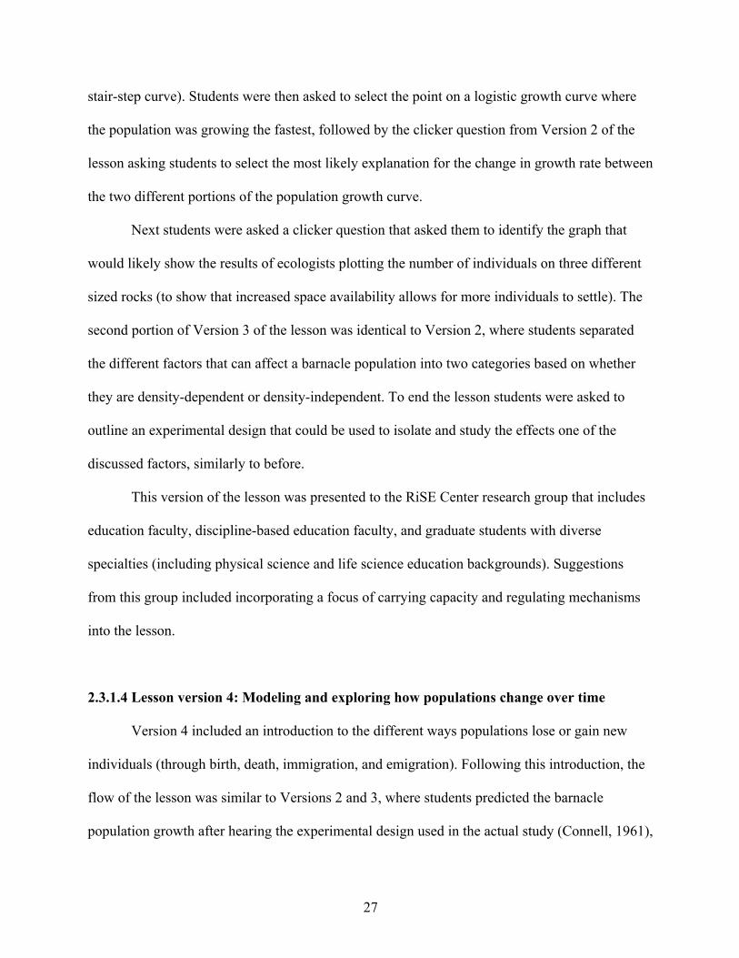
2.3.1.4 Lesson version 4: Modeling and exploring how populations change over time

Version 4 included an introduction to the different ways populations lose or gain new

individuals (through birth, death, immigration, and emigration). Following this introduction, the

flow of the lesson was similar to Versions 2 and 3, where students predicted the barnacle

population growth after hearing the experimental design used in the actual study (Connell, 1961),

28

selected the graph that resembled their prediction from four growth curves (linear, exponential,

logistic, and a stair-step curve), answered clicker questions addressing the change in growth rate

observed in the barnacle population over time, and separated the factors affecting barnacle

populations into two categories based on whether they were density-dependent and/or density

independent. The last section of the lesson where students were asked develop an outline of an

experiment to test the effects of one of the discussed factors on barnacle population size was

simplified. Specifically, students were presented with three experimental questions and asked

what they would change in the experimental design used to observe the effects of space

limitation (as worked through in class) to observe the effects of predation, competition, and

temperature on the barnacle population.

Version 4 was piloted in a General Ecology course at the University of Maine, Orono.

This course examines a broad range of ecological processes, principles, and examples in ecology.

Learning outcomes include: 1) describing abiotic and biotic factors that influence populations, 2)

applying ecological perspectives to problem-solving and decisions, and 3) analyzing ecological

and environmental problems to understand the roles of environmental drivers, biotic interactions,

and human actions on current and further ecological conditions. The lesson was implemented

mid-semester following discussion of population growth (carrying capacity and logistic growth

were introduced) but prior to discussion of the specific interactions within populations

responsible for such patterns in nature (i.e., intraspecific and interspecific competition). The class

was a 50-minute-long class with 41 students present.

Implementing the lesson in a classroom provided information about how students

interpreted the lesson and assessment questions. After the first round of piloting, it was apparent

that certain areas of the lesson needed to be reworked or removed. For example, the portion of

29

the lesson focusing on density-dependence and independence caused confusion among students.

Additionally, there was a clear disconnect in the importance of ecologists conducting such

experiments to determine how population growth is influenced in nature.

2.3.1.5 Lesson version 5: Modeling and exploring how populations change over time

Version 5 of this activity focused on growth curves, carrying capacity, regulating

mechanisms, and the four mechanisms that cause population sizes to change (birth, death,

immigration, and emigration), however the second half of the lesson was reworked to no longer

include the separation of factors into two categories based on density-dependence and

independence. Furthermore, a discussion of the importance of modeling and understanding

population growth for ecologists was added.

In this version of the lesson, students predicted the barnacle population growth over time

given the experimental design (Connell, 1961) and selected the graph that best depicted their

prediction from four growth curves (linear, exponential, logistic, and a stair-step curve). The four

potential graph choices were then individually discussed to highlight when populations in nature

might exhibit that type of growth. Next, students were presented with the actual growth curve

generated from the experimental data and asked to select the answer that best described what was

happening to the rate of settlement between two points on a logistic growth curve. Following

this, carrying capacity and the four mechanisms that cause population sizes to change (birth,

death, immigration, and emigration) were introduced. Next, students were asked to list different

abiotic and biotic factors that can influence those four mechanisms, such as competition,

predation, disease, reproductive ability, space availability, etc. The instructor discussed each of

the listed abiotic and biotic factors while keeping the experimental design in mind, to determine

30

which factor most likely caused the growth observed in the barnacle population in the month-

long study. For example, predation is a biotic factor that can influence the barnacle population,

however because of the cages placed on the rocks to prevent predators in the experimental

design, is not likely the cause of the observed barnacle population growth. Students were

presented with the conclusion of the study, that space availability was likely the factor

responsible for the barnacle populations exhibited growth. This version of the lesson ended with

students outlining an experiment to determine how predation might influence the barnacle

population.

Version 5 of the lesson was piloted in BIO 465, Evolution, at the University of Maine,

Orono. This course investigated the origin and development of evolutionary theory and the

mechanisms that bring about the genetic differentiation of groups of organisms. The lesson was

implemented near the end of the semester and was presented to 71 students. This round of

piloting revealed that the second half of the lesson was still weak. The discussion of the factors

influencing barnacle population growth (birth, death, immigration, and emigration) was

incomplete and the portion of the lesson asking students to design an experiment to test the effect

of predation on the barnacle population was not well received in the classroom as a result of the

lack of structure. For example, students were unsure of what information they were expected to

include.

2.3.1.6 Lesson version 6: Modeling and exploring how populations grow over time

Version 6 of the lesson integrated feedback from the second pilot to continue to

strengthen the content and flow of the lesson. In this version, background information on

barnacles and the intertidal zone was covered, followed by the introduction of abundance and

31

density (two measures used by ecologists to measure population size). Next students predicted

the barnacle population growth over time given the experimental design (Connell, 1961) and

selected the graph that best depicted their prediction from four growth curves (linear,

exponential, logistic, and a stair-step curve). The four growth curves were discussed individually

and students answered the same clicker question, selecting the answer that best described what

was happening to the rate of settlement between two points on a logistic growth curve.

In this version of the lesson students were still presented with the four common

influences on population growth (birth, death, immigration, and emigration), however after being

introduced with the terms, the students were asked to generate an equation to calculate

population size using the four influences. Following the development of the equation, students

were asked to list different abiotic and biotic factors that affect each of the four influences.

Similarly to the previous lesson, the instructor walked through the experimental design to discuss

if each of the abiotic factors were likely responsible for the growth exhibited by the barnacles.

Through this exploration of biotic and abiotic factors, the instructor guided students to the

conclusion that space is likely responsible for the decrease in growth overtime for the barnacle

population. The experimental design portion of the lesson was simplified, providing students

with a breakdown of the experimental design used in the seminal barnacle population growth

study to mirror, asking students to outline an experiment to investigate the effects of predation on

barnacle population growth. To conclude, four growth curves (linear, exponential, logistic, and a

stair-step curve) of organisms found in nature were presented to the students to highlight the

importance of these growth curves.

This version of the lesson was presented to the Smith laboratory for feedback.

Suggestions from this group included shortening the length of the lesson; adding additional

32

clicker questions, particularly to assess student understanding of density and abundance;

simplifying the generation of the equation to relate birth, death, immigration, and emigration;

and lastly to strengthen the section on the importance for ecologists to study population

dynamics.

2.3.1.7 Lesson version 7: Modeling and exploring how populations grow over time

Version 7 of the lesson focused on three main parts: 1) What affects the size of barnacle

populations and how the grow over time? 2) Why is it important for ecologists to study

population dynamics? and 3) What is the practical importance of population dynamics? Overall,

the first portion of the lesson (what affects the size of barnacle populations and how they grow

over time) remained the same as previous versions, however the introduction to barnacles and

the intertidal zone was shortened and a clicker question was developed to assess student

understanding of the measures of population size (density and abundance). Additionally, in this

version of the lesson, the breakdown of each of the four growth curves (linear, exponential,

logistic, and a stair-step curve) was removed. After introducing the four main influences on

population size (birth, death, immigration, and emigration), students were asked to select from

equations that best modeled changes in population size using those terms. This version of the

lesson walked students through each of the potential factors that might influence birth, death,

immigration, and emigration to determine why the barnacle population growth resulted in a

logistic growth curve, similarly to previous lessons.

After determining the most likely cause of population stabilization over time, the focus of

the lesson shifted to the importance of studying population dynamics. This portion of the lesson

introduced endangered species and the importance of modeling those populations. By discussing

33

three different success stories of endangered species, the instructor demonstrated the importance

of understanding population dynamics for aiding in the rebound of those populations.

This version of the lesson was presented at the RiSE Center conference where over 50

high school teachers provided feedback. Feedback from this group was positive, most teachers

stated that it was a lesson they would want to use in their classroom to teach their students about

population growth. After receiving the feedback, it was decided the lesson was well suited for a

high school classroom, however the content needed to be modified to increase difficulty before

being implemented in an undergraduate classroom.

2.3.1.8 Lesson version 8: Describing and modeling populations over time

Version 8 of the lesson was modified to make the lesson better suited for an

undergraduate classroom. The first part of the lesson remained the same- students were presented

with the background information on seminal study used to measure barnacle population size

(Connell, 1961) and were asked to make a prediction of barnacle population growth over time,

however in this version of the lesson students were only given three graphs to choose from

(linear, exponential, and logistic). Additionally, rather than giving the students the results from

the experiment, students were given the data and asked to generate a graph to determine how the

barnacle population changed over time.

Following the graphing exercise, students were presented with the equations used to

calculate growth rate for each of the three main growth curves. Students then answered a clicker

question targeting understanding of how the rate of growth changes over time in all three growth

curves (linear, exponential, and logistic). Next, each growth curve and equation was broken

down to discuss the similarities and differences between the three. In order to assess students’

34

abilities to use the logistic growth curve to determine what happens to the growth rate as the

population size approaches carrying capacity, students were presented with a clicker question.

This version of the lesson focused on the importance of collecting and analyzing descriptive

data, using mathematical models to simplify the complexity of ecology, and the implications of

carrying capacity on population growth.

Version 8 of the lesson was presented to the Smith laboratory for one additional round of

feedback before implementing it in the BIO 100 introductory biology course at the University of

Maine. At this meeting the feedback was minor and focused mainly on small visual changes to

slides.

2.3.1.9 Lesson version 9: Describing and modeling populations over time

The final lesson was implemented in an introductory biology course at the University of

Maine, Orono where a total of 433 students participated in the pre-test, lesson implementation

which includes several formative assessment clicker questions, exam equations, and a post-test.

The format of the final lesson and results from this implementation are discussed in depth in

Chapter 3.

2.4 Recommendations for developing lessons

The iterative process of developing this lesson provided me with knowledge and

confidence in developing similar lessons in the future. This section highlights the important steps

to follow to generate a lesson that targets student understanding in the classroom based on what I

have learned through this process (Table 2.5).

35

Step Description Timeline

I. Identify an area where students struggle or where instructional material is needed.

This can be done through previous research, personal experience, review of the available educational literature, or a combination of the three.

4-7 days

II. Research student understanding of the topic and relevant skills.

Research educational literature on student thinking and conceptual difficulties when learning about the chosen topic.

4-6 days

III. Research the current materials available to teach the chosen topic.

Review the available textbooks, online lectures, and online lessons to determine how others approach teaching the topic.

4-7 days

IV. Develop learning outcomes for the lesson.

Think about what you want students to be able to do upon completion of the lesson.

2-5 days

V. Develop an assessment tool to assess student understanding of the learning outcomes.

Develop an assessment tool to successfully assess all learning outcomes.

2+ months

VI. Develop the lesson to target student understanding of the developed learning outcomes based on current knowledge of student thinking.

Using the information gained through the literature, textbook, online lesson, and online lecture review create a lesson to target the developed learning outcomes.

3+ months

Table 2.5: Timeline for the development of a lesson. Outline of the necessary steps to develop a lesson to address students’ conceptual difficulties for a specific topic. 2.4.1 Important steps and timeline for development

When developing a lesson to promote significant learning experiences for students, I

recommend employing the “backwards design” process, which begins with a vision of the

desired results in mind (Wiggins and McTighe, 1998). This process divides instructional

planning into three stages: 1) identifying desired results, 2) determining what constitutes

acceptable evidence of learning, and 3) planning the learning experiences and instruction

(Wiggins and McTighe, 1998).

Identifying areas of persistent struggle for students and incorrect thinking students

possess when learning helps to determine what is worthy of requiring student understanding

(Stage 1; Wiggins and McTighe, 1998). There are several ways to identify where students

persistently struggle. One is based on classroom experience and interactions with students.

36

Another is using the published literature, such as the information of particular areas where

students struggle in population ecology (see Chapter 1).

Once the topic of the lesson has been determined, it is important to examine multiple

textbooks to understand how others present the material, allowing you to gain a sense of the flow

of the lesson as well as what terms and concepts should be stressed (Table 2.1). Furthermore, it is

recommended to review available online lectures (Table 2.2.) and lessons (Table 2.3) covering

the topic to observe how others are presenting this topic to their students. This step is crucial, as

it allows you to see how others are taking the content in the textbook to teach the material.

Following the literature, textbook, and online lesson review, I recommend developing the

learning outcomes: what do you want students to be able to do at the completion of the lesson?

(Stage 2; Wiggins and McTighe, 1998). Learning goals are used to communicate the key ideas of

a course/lecture/lesson and the level at which students should understand those ideas in

operational terms (Smith and Perkins, 2010). Typically, learning goals take the form of “at the

end of the course/lecture/lesson, students will be able to…” followed by a specific verb and task

(Smith and Perkins, 2010). For example, a topic-level learning goal from an introductory

genetics course at the University of Colorado (CU) was “At the end of this lesson, students will

be able to distinguish between different modes of inheritance (Smith and Perkins, 2010). Based

on experiences working in groups of faculty to formulate learning goals, Smith and Perkins

(2010) suggest six steps for creating useful learning goals that are outlined in in Figure 2.3.

37

Figure 2.3: Suggested checklist for developing useful learning goals (Smith and Perkins, 2010).

Research has revealed that learning goals are beneficial for students, instructors, and

alignment of courses (Simon and Taylor, 2009; Smith and Perkins, 2010). For example, to

explore the impact of learning goals on students and instructors in the classroom, instructors

from three courses at the University of British Columbia wrote individual learning goals in the

form of, “At the end of this lecture/ topic I will be able to…” and presented the learning goals to

students as part of their lectures (Simon and Taylor, 2009). Following the lessons, students were

asked to complete up to five copies of the sentence, “For me, the use of learning goals in this

course is…” and student responses were analyzed and separated into categories such as Study,

Exams, Lecture, General Positive, and Negative. Additionally, the instructors involved in the

38

study were interviewed to examine their views of learning goals. Overall, results from the study

suggest that there are benefits for writing and sharing learning goals. Responses from students

showed that nearly all students involved in the study found learning goals to be valuable, with

most mentioning the largest value being that they helped students “know what I need to know for

a course.” Similarly, results from instructor interviews suggest that learning goals enhanced

communication, as instructors stated the learning goals provided a method to clearly outline the

importance concepts and materials in the class for students.

After developing learning goals, instructors should determine how achievement of the

learning goal will be assessed (Figure 2.3, step 2; Wigging and McTighe, 1998). It is important

that the learning goals and assessments are aligned at a similar level of cognitive understanding

expected of students (Smith and Perkins, 2010; Bloom and Krathwohl, 1956). For example, if the

learning goal asks students to apply knowledge to unfamiliar situations, the assessment questions

should assess students’ ability to do just that. Instructors can use formative and summative

assessments to monitor student success in the classroom. Formative assessment monitors student

learning to provide feedback that can be used to improve instructors teaching methods and

student learning (Yorke, 2008), while summative assessment evaluates student learning at the

end of an instructional unit or course (Teaching excellence and education innovation, 2008).

Formative assessments are typically low stakes and include but are not limited to using clicker

questions, concept maps, and research proposals, while summative assessments are high stakes

and can include midterm exams, final projects, and papers (Teaching excellence and education

innovation, 2008).

Once useful learning goals and assessment tools have been created, the next step is to

develop at lesson to promote understanding, interest, and competency in the subject matter is

39

next (Stage 3; Wiggins and McTighe, 1998). The development of the lesson will be most

successful if it goes through multiple rounds of edits. I recommend giving the lesson to

colleagues and students, allowing for feedback on the content, level of difficulty, and

effectiveness of the lesson. During this process, it is important to engage with content experts

who provide feedback on the content covered and educational specialist who can give feedback

on the success of the teaching methods used. During this process, I recommend presenting the

lesson as if you were giving it to students in the classroom, allowing you as the developer to

observe how the lesson is received, and allowing the participants to gain a greater understanding

of student interaction with the material.

Prior to presenting the lesson for feedback it is important to have specific areas where

you wish to receive feedback. Written and oral feedback are both beneficial, therefore I suggest

using audio and/or video recordings and requesting written feedback from participants. To meet

with a diverse set of faculty with busy schedules, I recommend requesting feedback during

already established journal club/ seminar times or using an online poll system to determine the

most convenient meeting time. After receiving such feedback, but prior to finalizing the lesson,

piloting the lesson to students can allow for a deeper understanding of student interpretation and

interaction with the material. After piloting the lesson, I suggest going through a final round of

edits and feedback.

40

CHAPTER 3

AN ACTIVE-LEARNING LESSON THAT TARGETS STUDENT UNDERSTANDING

OF POPULATION GROWTH IN ECOLOGY

3.1 Overview

As a part of this thesis project, the active-learning population ecology lesson has been

submitted for publication in CourseSource, an open-access journal of peer-reviewed teaching

resources for undergraduate biological sciences. This journal publishes articles that are organized

around courses in biological disciplines and aligned with learning goals established by

professional societies. The third chapter of this thesis is the manuscript submitted to

CourseSource.

3.2 CourseSource abstract

Effective teaching and learning of population ecology requires integration of quantitative

literacy skills. To facilitate student learning in population ecology and provide students with the

opportunity to develop and apply quantitative skills, we designed a clicker-based lesson where

students investigate how ecologists measure and model population size. This lesson asks students

to “engage like scientists” as they make predictions, plot data, perform calculations, and evaluate

evidence. The lesson was taught in three sections of a large enrollment undergraduate class and

assessed using a pre/post-test, in-class clicker-based questions, and multiple-choice exam

questions. Student performance increased following peer discussion of clicker questions and on

post-test questions. Students also performed well on the end-of-unit exam questions.

41

3.3 Scientific teaching context

3.3.1 Learning goals

How do populations change over time? (from the CourseSource Ecology Learning

Framework, http://www.coursesource.org/courses/ecology)

Students will know that many different growth curves and patterns exist for organisms in

nature. They will understand that modeling helps to describe and predict population

growth over time.

3.3.2 Learning objectives

Students will be able to:

• Calculate, graph, and compare the population density and abundance.

• Identify whether a growth curve describes exponential, linear, and/or logistic

growth.

• Describe and calculate a population’s growth rate using linear, exponential, and

logistic models.

• Explain the influence of carrying capacity and population density on growth rate.

3.4 Introduction

Quantitative reasoning and literacy skills are essential for many careers, particularly those

in biology where individuals encounter a diversity of challenges that require an application and

integration of approaches NRC, 2003; AAAS, 2009). To prepare students to address these

challenges, which span a variety of sectors including health, education, the environment, and

42

complex social issues; biology education researchers have advocated integrating quantitative

skills with biology content (Speth et al., 2010; Hester et al., 2014; Bravo et al., 2016). This

integration gives students the opportunity to practice posing questions, analyzing and interpreting

evidence, developing models, and generating testable predictions (NRC, 2002; NRC 2009).

Previous studies have revealed that undergraduate biology students struggle with higher-order

quantitative thinking (e.g., analyzing, evaluating, and drawing conclusions), particularly with

generating graphs from raw data (Speth et al., 2010; Picone et al., 2007); interpreting bar graphs

and scatterplots (Speth et al., 2010); understanding independent and dependent variables (Picone

et al., 2007); summarizing trends from data with variation (Picone et al., 2007; Kitchen et al.,

2003); and articulating data driven arguments (Speth et al., 2010). Introductory biology students

also have difficulty performing simple calculations (such as calculating a mean) and representing

calculations graphically (Speth et al., 2010).

Population ecology is a topic well-suited for the development of quantitative reasoning

and literacy skills. At both the introductory and advanced levels, students are asked to model

population growth using graphs, measure population size, and estimate carrying capacity (Urry et

al., 2014; Cotgreave and Forseth, 2002). However, students often struggle with integrating

quantitative skills with conceptual understanding and practical application (Urry et al., 2014;

Cotgreave and Forseth, 2002). For example, undergraduate students have incorrectly predicted

that a population would likely exceed carrying capacity if a non-limiting factor increased

(Summers et al., submitted) and that all population sizes will level off regardless of the resources

available (D’Avanzo, 2003). They have also explained that competition only occurs between

organisms of the same species (Summers and Smith et al., submitted; Munson, 1994). Although

instructional tools currently available target some of these persistent conceptual difficulties (Hale

43

and McCarthy, 2016; Jeanne, 2003; Beckstead et al, 2011; Aronhime et al., 2013; Glase and

Zimmerman, 1991; Langin et al., 2009), there is a need for materials explicitly designed to

investigate student thinking and learning progressions. In additional, available instructional

materials on this topic are also largely computer models and lab-based activities, leaving a need

for tools that integrate quantitative skills in a large-enrollment format.

Here we describe an interactive in-class lesson that targets conceptual difficulties in

population ecology and seeks to develop students’ quantitative reasoning. This 50-minute

clicker-based lesson focuses on exploring population growth in a barnacle population using

authentic data from a seminal study in ecology (Connell, 1961). Throughout the lesson, students

predict, plot, calculate, and interpret data to learn the methods used by ecologists to measure,

describe, and model population growth.

3.5 Lesson background information

3.5.1 Intended audience

This lesson is intended for undergraduate introductory biology courses. It was given to

students in a large enrollment Introductory Biology course at the University of Maine (n=766;

students divided into three class sections). In this class, the mean SAT Math score was 525

(range from 320-770; 87% of students took the SAT) and mean ACT Math score was 23 (range

14-33; 18% of students took the ACT).

3.5.2 Required learning time

This lesson was designed for a 50-minute class period.

44

3.5.3 Pre-requisite student knowledge

Before participating in the lesson, students participated in one class where the following

topics were discussed: abiotic and biotic factors responsible for determining population size, the

definitions of carrying capacity and regulation, and different examples of populations that exhibit

logistic and exponential growth. They were also asked to complete an assigned textbook reading

(Urry et al., 2014) that introduced population ecology and an overview of biotic and abiotic

factors, density, exponential population growth, logistic and exponential growth curves and

equations, carrying capacity, and density-dependent regulation.

3.5.4 Pre-requisite teacher knowledge

We recommend that instructors are familiar with how ecologists study population growth

and the main concepts covered in the lesson (measurements of population size; the equations that

describe linear, exponential, and logistic growth; the role of carrying capacity; and examples of

different growth models and their applications). Instructors will also benefit from basic

knowledge about barnacles and the intertidal zone. Information about each concept, barnacles,

and the intertidal zone are included in the lesson slides (Appendix A). Recommended population

ecology resources are also provided in Appendix B.

We also suggest that instructors familiarize themselves with common and persistent

conceptual difficulties related to population growth. We used the Ecology and Evolution

Measuring Achievement and Progress in Science or EcoEvo-MAPs assessment tool (Summer et

al., submitted) at the beginning of this course to identify some of the ecology and evolution

concepts that cause our students to struggle.

45

3.6 Scientific teaching themes used in the lesson

3.6.1 Active learning

Students are actively engaged in their learning throughout the lesson. Students make

predictions, answer clicker questions, engage in peer discussion, participate in group problem-

solving, answer questions in their own words on a worksheet, and respond to instructor

questions. The instructor who taught this lesson was observed using the Classroom Observation

Protocol for Undergraduate STEM (COPUS) (Smith et al., 2013). This observation protocol uses

a series of codes to characterize instructor and student behavior in the classroom and documents

those behaviors in two-minute intervals throughout the duration of the lesson (Smith et al., 2013;

Smith et al., 2014). The summary of COPUS results (Figure 3.1) highlights the diversity of

student-centered instructional practices and student participation in this lesson. For example,

throughout the lesson more than 25% of the codes were “students talking to the class” (asking

and answering questions) and more than 25% of the codes were “students working” (working

individually, answering clicker questions, and working in groups). Similarly for the instructor,

nearly 75% of the codes were “guiding” (posing questions to students, asking clicker questions,

following up with students, and moving and guiding).

3.6.2 Assessment

Students were assessed using formative and summative questions aligned with the

learning outcomes: quantifying population size, plotting and predicting population growth,

calculating growth rate, and incorporating carrying capacity in logistic growth curves. We used

clicker-based questions for formative real-time assessment of student understanding during the

46

lesson. Student responses are included in the lesson plan and in Appendix C. Summative

assessment of student understanding included a pre/post-test and exam questions. The pre- and

post-test consisted of ten multiple-choice questions and were administered online. Students had

one day to complete the pre-test immediately preceding the lesson. Students were given five days

to complete the post-test, starting five days after the lesson. Pre/post-test questions are included

in Appendix D. Students also answered three multiple-choice exam questions three days after the

lesson. Multiple-choice exam questions are provided in Appendix E.

Figure 3.1: COPUS results from the lesson implementation. Average collapsed Classroom Observation Protocol for Undergraduate STEM (COPUS) (Smith et al., 2013; Smith et al., 2014) codes from three sections of a University of Maine introductory biology course in which this lesson was used. Collapsed student codes: Receiving (Listen- Listening), Students Working (Ind- Individual Work, CQ- Clicker Question Discussion, WG- Worksheet Group Work), Students Talking to Class (AnQ- Answering Question, SQ- Student Question). Collapsed instructor codes: Presenting (Lec- Lecturing, RtW- Real Time Writing), Guiding (FlUp-Follow-up, PQ- Posing Questions, CQ-Clicker Question, AQ-Answer Question, MG-Moving and Guiding), Administration (Adm- Administration).

47

3.6.3 Inclusive teaching

This lesson seeks to create a learning environment where students’ academic, social, and

cultural backgrounds can be an asset to their learning. This inclusive teaching environment was

fostered through incorporating a variety of different teaching methods to meet the needs of

students with diverse learning styles, abilities, and backgrounds (Armstrong, 2011; Inclusive

teaching strategies, 2016). For example, the concepts were presented and available to students on

projected slides, the student worksheet, and through instructor and peer-led discussion. When

questions were presented, students were given the opportunity to first think and write on their

own, then discuss in small groups, and finally report out to the entire class. In addition, we used

an anonymous response system (clickers) with peer discussion to reduce student discomfort

(Martyn, 2007) and promote a collaborative learning environment (Crouch and Mazur, 2001;

Smith et al., 2009; Smith et al., 2011).

3.7 Lesson plan

This lesson is designed for a 50-minute lecture and is intended to introduce students to

quantitative skills used in population ecology, and can follow an introduction to population

ecology (in a previous class or as a pre-class assignment). The progression of the clicker-based

lesson with estimated timing is provided in Table 3.1.

48

Activity Description Estimated time Preparation for Class Introduction to population ecology concepts and terminology

Prepare students to define and recall the following terms: a. Density a. Abundance b. Carrying Capacity c. Density dependence d. Linear, exponential, and logistic growth Prior to this lesson, students should be exposed to the concepts listed above either through reading or information presented in a previous class.

Pre-test Provide students with the pre-test to complete before the start of class.

~ 20 min

Class Session- Progressing through the Activity 1. Introduction and assessing prior knowledge

Slides 1-5

1. Provide background information on the intertidal zone and barnacles. 2. TPSQ1: Students brainstorm in small groups followed by a facilitated classroom discussion of abiotic and biotic influences on barnacle population size.

~10 min

2. Quantifying population size

Slides 6-10

1. Introduce density and abundance as two ways that ecologists can measure population size. 2. CQ1: Students answer and discuss a clicker question that reinforces the difference between measuring density and abundance. Following facilitated group discussion, provide an explanation of how to calculate density and abundance.

~5 min

3. Predicting and plotting population growth

Slides 11-16

1. Introduce the relevant methodology used in Connell, 1961 to study barnacle population size (Connell, 1961). 2. TSPQ2: Students graph their prediction of barnacle population growth over the 30-day experiment. 3. CQ2: Students answer and discuss a clicker question selecting the growth curve that most resembles their prediction of barnacle population growth. 4. TPSQ3: Students use data from the scientific study to plot barnacle population growth. 5. CQ3: Students answer a clicker question selecting the growth curve that most resembles the plot generated from the data.

~10 min

Table 3.1: Progression through the clicker based lesson. Progression through the clicker-based lesson with approximate time stamps. Each classroom-discussion open-response TPS question opportunity is identified by “TPSQ” and each Clicker Question TPS opportunity is abbreviated “CQ” for Clicker Question. Pre-test, lecture slides, and post-test are available in the Appendices A and D.

49

Activity Description Estimated time 4. Identifying and discussing growth rate

Slides 17-22

1. Introduce growth rate and how it differs between linear, exponential, and logistic growth curves. 2. CQ4: Students answer and discuss a clicker question investigating how the growth rate is changing over time in all three growth curves. Expand on the discussion by showing the different equations used to describe the growth rate and emphasize how growth rate differs between each (constant over time in linear, increasing over time in exponential, and increasing initially, then decreasing in logistic). 3. Demonstrate how to calculate the growth rate at different time-points or population sizes for a linear and exponential growth curve. Explain the variables used in linear and exponential growth models: population size (N) and time (t), and the intrinsic rate of increase (r). Introduce the technique of changing the values of the variables to examine how the growth rate changes. Emphasize how the exponential equation results in an increasing growth rate over time.

~8 min

5. Incorporating carrying capacity

Slides 23-29

1. Identify predicted carrying capacity on the Connell, 1961 data plot. Define regulating mechanisms and ask students to volunteer likely regulating mechanisms for the barnacle population. 2. Explain the variables used in the logistic growth model: intrinsic rate of increase (r), population size (N), and carrying capacity (K). Emphasize how K influences the growth rate in this model. 3. CQ5: Students answer and discuss a clicker question about calculating the growth rate of the barnacle population over time using given values for r, K, and N. Provide an example of how to calculate the growth rate for one population size in a logistic growth curve. Emphasize how the equation models what happens to the growth rate as the population approaches carrying capacity (the growth rate increases initially, is the fastest at half the carrying capacity, and decreases as the population approaches carrying capacity). 4. Show students the growth rates for the plot of the Connell, 1961 data. Focus on how the growth rate resembles the trend of logistic growth - increasing then decreasing as the population approaches carrying capacity.

~10 min

Table 3.1: Continued.

50

Activity Description Estimated time 6. Synthesis

Slides 30-34

1. Summarize the three mathematical models discussed in the activity and how the change in growth rate differs for each. 2. Explain the applications of growth models to economic, medical, and conservation predictions and decision-making. 3. TPSQ4: Students use data from four different types of organisms (bristlecone pine trees, grey wolves, bacteria, and red foxes) to describe and discuss each population’s growth. Students identify if abundance or density is shown, what is happening to the population over time (increasing, decreasing, etc.), and if the growth curve most closely resembles linear, exponential, or logistic growth. Facilitate a whole-class discussion focused on problem-solving techniques. For example, using the y-axis to determine if abundance or density is measured; considering population size and rate of growth separately; and identifying the role of carrying capacity in producing logistic growth. 4. Review the learning outcomes and summary slide of the activity and answer any student questions.

~7 min

Follow-up Post-test Provide students with the post-test following the activity. ~20 min Table 3.1: Continued.

3.7.1 Pre-class preparation

We recommend that students are familiar with and able to recall the following terms

before the lesson: density; abundance; carrying capacity; density dependence; and linear,

exponential, and logistic growth (Appendix B). This preparation can be achieved through prior

readings, homework assignments, or lectures.

Instructors will need to facilitate conversations among students during this lesson.

Additional instructional resources on the content and quantitative skills covered are provided in

Appendix B.

51

3.7.2 Think-Pair-Share and use of clickers

Think-Pair Share (TPS) is a classroom-based active learning strategy in which students

think about a problem posed by an instructor individually, work in pairs to solve the problem,

and finally share their ideas with the entire class (Kothiyal et al., 2013). This model allows

students to individually think about the questions posed, reflect on their own thinking, and obtain

immediate feedback from their peers and instructor (Lyman, 1987). During the in-class lesson,

students answered several questions using the TPS model. Clickers were also used to facilitate

TPS opportunities. Students first answered individually (“think”) followed by discussion with a

neighbor and revote (“pair”). After the revote, the instructor asked for students to volunteer their

thinking (“share”) and then discussed the correct answer and student thinking. This combination

of peer and instructor-led discussion has been shown to result in greater student gains than either

peer discussion or instructor explanation alone (Smith et al., 2009). In the instructor slides and

student worksheet, each classroom-discussion open-response TPS question opportunity is

identified by “TPSQ” and each Clicker Question TPS opportunity is abbreviated “CQ” for

Clicker Question (Appendix A, Appendix F). Specific advice on the administration of each of

these questions is given in the “Progressing Through the Lesson” section and in the notes section

of the lesson slides.

3.7.3 Progressing through the lesson

3.7.3.1 Introduction and assessing prior knowledge (~10 minutes)

The lesson begins with an overview of population dynamics and engaging students’ prior

knowledge about barnacles. The instructor first defines population dynamics and informs

52

students that they will be learning some of the methodology used by population ecologists:

collecting and analyzing descriptive data and generating and evaluating mathematical models

(Appendix A). The instructor then explains that although ecologists in general seek to understand

how all organisms in an ecosystem interact, population ecologists approach this goal by focusing

on individual populations that they can observe and manipulate with experiments (Appendix A).

The instructor can also introduce the seminal role that barnacles played in developing the field

and methodology of population ecology and also why barnacles are a good system for studying

population growth (Connell, 1961). Since most of the lesson focuses on barnacle population

growth, the instructor next gives students the opportunity to engage their prior knowledge about

barnacle biology and what affects their population size.

TPSQ1. What affects barnacle population size?

For approximately four minutes, students brainstorm in small groups and write on their

worksheet factors they think might affect barnacle population size (Appendix A). This time

allows students to review and ask questions about barnacles before seeing data related to

barnacle population growth. In our introductory biology course students mentioned: temperature,

salinity, human disturbance (crushing), competition, food availability, exposure to the air, wave

action, predation, and disease as likely factors affecting barnacle population size. Typical

questions that arose about barnacles included, “How long can barnacles live outside of the

water? (answer: up to about 6 weeks); “Do barnacles reproduce sexually?” (answer: yes, most

species of barnacles are hermaphroditic); and “What preys on barnacles?” (answer: fish, limpets,

crabs, sea stars, and marine snails such as whelks).

Following small group discussion, the instructor can solicit answers from students. If

desired, the instructor can write these answers on a board and identify biotic versus abiotic

53

factors. A summary slide of factors that students mentioned in the lesson is provided (Appendix

A). To transition to the next section of the lecture, the instructor focuses students’ attention to the

variable of interest on the summary slide – the number of barnacles.

3.7.3.2 Quantifying population size (~5 minutes)

This section of the lesson focuses on how ecologists measure and describe population

size. The instructor first introduces density and abundance, explaining that whether density or

abundance is used depends on the organism and study design (Appendix A). For example, when

observing a population of elephants in the savannah, abundance is likely a more useful measure

of population size because you can easily count every individual. If, however, you are observing

bacteria in a flask, you would measure density due to the constraints of counting every single

individual. Since having a clear understanding of these two measurements is important, the

instructor next gives students the opportunity to compare and calculate density and abundance.

CQ1. Which of the following statements describes the two study sites below?

Students observe a diagram and compare the density and abundance of barnacles. Using

their clicker, they select from the following answer choices: A) site two has a greater abundance

and density than site one; B) site one has a lower abundance but equal density to site two; C) site

one has a lower abundance but greater density than site two; or D) the density and abundance are

equal for both sites (Appendix A). After responding to the question individually, students discuss

in small groups and revote. During this time, the instructor should encourage students to discuss

their reasoning and how they calculated density and abundance. In our class, 70% of students

answered correctly before peer discussion (answer C) and 93% were correct following peer

54

discussion (Appendix B). These results suggest that students had a good understanding of density

and abundance after receiving the definition of both.

After small group discussion, the instructor can ask students to describe how they arrived

at their answer. In our class, students described two different ways of determining the correct

answer. Some students calculated the density while others used the diagram to visually compare

the density and abundance of barnacles in each study site. The clicker question was designed to

allow students to conceptually answer the question without calculating the density of the two

study sites. After restating different problem-solving techniques, the instructor can provide an

explanation of how to calculate density and abundance using mathematical equations (Appendix

A).

3.7.3.3 Predicting and plotting population growth (~10 minutes)

Next, students are asked to make a prediction using a graph and plot data of population

growth over time. The instructor first introduces the methodology used by Connell, 1961 to study

barnacle population growth in the intertidal zone (Appendix A). Emphasis on the following

experimental features is important for this lesson: 1) the author measured the density of the

population (y-axis); 2) the study was conducted over two months (x-axis); and 3) cages were

used to prevent predation during the experiment (Connell, 1961). To provide students with the

opportunity to think about the x-and y-axes on the graph, and also how barnacle populations

might grow over time, the instructor next asks students to predict barnacle population size over

the course of the experiment.

55

TPSQ2. Draw on your paper what you would expect the growth of this population to look

like over the 30-day experiment.

CQ2. Select the growth curve that most resembles your prediction for barnacle population

growth.

Students will use the blank graph on their worksheet (with the y- and x-axis provided and

labeled) to predict barnacle population size over the course of the study (Appendix A; Appendix

F). To easily quantify student predictions, the instructor gives the students a clicker-question

(CQ2) asking them to individually vote for the growth curve – A) linear, B) exponential, or C)

logistic – that most resembles their prediction (Appendix A). During the individual vote in the

lesson, students chose all three growth curves (23% linear, 43% exponential, and 34% logistic).

Students then talk with their peers and revote using their clickers. The instructor can encourage

students to discuss their reasoning and what they think may influence the type of growth shown

in the curve they selected. Following peer discussion in the lesson, 7% selected a linear growth

curve, 33% chose exponential, and 60% of students voted for the logistic.

After peer discussion, the instructor can solicit answers from students by having them

raise their hands and share their initial prediction and reasoning. In the lesson, student reasoning

for each of the growth curves included: linear - “The population will increase steadily over

time,” exponential - “I don’t know what the carrying capacity of the rock is, there is not enough

information to know if or when the population will level off,” logistic - “Since the study was

conducted on a single rock, I figured eventually the barnacles would run out of space, and there

would be no more room for additional barnacles to settle, therefore the graph would level off.”

After discussing students’ responses, the instructor provides students with the experimental data

to plot and compare to their prediction.

56

TPSQ3. Use the data provided to plot the barnacle population growth.

CQ3. Select the growth curve that most resembles the curve you generated from the data

provided.

Students use data from Connell, 1961 to plot barnacle population size over time on their

worksheet (Appendix A; Appendix F). To check that students are plotting the data correctly, the

instructor gives the students a clicker question (CQ3) where they select the growth curve – A)

linear, B) exponential, or C) logistic – that most resembles their plot of the provided data (S1,

slide 15-16). In our class, 99% of students answered correctly during the individual vote and the

instructor skipped peer discussion (Appendix C). The instructor next says that while logistic

growth is common, other mathematical models (e.g., linear and exponential) can be used to

describe growth in populations. Also, since there are periods of linear and exponential growth in

the barnacle data, all three of types of growth will be discussed further.

3.7.3.4 Identifying and comparing growth rate (~8 minutes)

This part of the lesson targets the mathematical equations used to describe growth rate.

The instructor first defines growth rate and then describes how it differs for the three growth

curves (linear, exponential, and logistic), showing, but not yet explaining the three mathematical

equations (Appendix A). The instructor can emphasize that one thing ecologists may be

interested in determining is how the growth rate changes, or might change, over time. The

instructor then uses a clicker question to help students distinguish how growth rate differs in the

three growth curves.

57

CQ4. The growth rate (or change in the population density) is:

Students use a diagram of the three different growth curves (linear, exponential, and

logistic) and infer how the growth rate is changing over time in each. Using their clickers (CQ4),

students select from the following answer choices: A) increasing over time in all three growth

curves; B) increasing over time in the linear and exponential growth curves only; C) constant

over time in all three growth curves; or D) constant in the linear growth curve and changes over

time in the exponential and logistic growth curves (Appendix A). In our class, 74% of students

answered correctly (D) before peer discussion, while 15% selected choice B. After peer

discussion, the number of correct responses increased to 86%.

After small group discussion, the instructor solicits answers by having students raise their

hands and explain how they arrived at their answer. In the lesson, student reasoning for selecting

choice A included: “It looks like the growth rate is increasing in all three graphs, because the

population size is getting larger over time.” Reasoning for B included: “The population is

increasing over time in the linear and exponential growth curves, however it is leveling off in the

logistic.” Reasoning for the correct answer D included: “If you look at the slope of the line, you

will see that it is constant in the linear growth curve, however it changes over time in both the

exponential and logistic growth curves.”

Next, the instructor demonstrates how to calculate the growth rate at different time-points

and population sizes using a linear and exponential growth model (Appendix A). The instructor

should first explain the variables used in the linear growth model: population size (N) and time

(t), and introduce the technique of changing the values of the variables in the equation to see how

the growth rate changes. By selecting two points on the linear growth curve, the instructor shows

58

the students how the growth rate is constant over time. This is also a good time to say that the

slope of the line is the growth rate.

The instructor then introduces the variables used in the exponential growth model:

population size (N), time (t), and the intrinsic rate of increase (r). The instructor describes the

intrinsic rate of increase (r) as a value that ecologists estimate. The instructor exaplains that the

simplest way to interpret r in the context of exponential growth is that if r=2/day, for every

barnacle present, two additional barnacles will be added per day. The instructor can then use the

technique of changing the values of the variables to see how the growth rate will vary. Here it is

important that the instructor to emphasize that in exponential growth as the population size

increases, the growth rate increases.

3.7.3.5 Determining the influence of carrying capacity (~10 minutes)

This section of the lesson addresses limitations to population growth. Using the Connell,

1961 data, the instructor provides an estimate of the carrying capacity (Appendix A). Here the

instructor highlights that the first portion of the graph resembles exponential growth, but that

there is a decrease in the growth rate as the barnacle population approaches ~80 barnacles per

cm2, which is an estimate of carrying capacity (Appendix A). The instructor defines regulating

mechanisms (those that influence population growth rate) and density-dependent regulation

(which occurs when population growth rates are influenced by the density of the population).

Here the instructor can ask students to volunteer likely regulating mechanisms for the barnacle

population. In our class students mentioned: food availability, predation, disease, and/or space.

Given the experimental set-up, where food is plentiful and predation is prevented, the most likely

regulating mechanism is space.

59

After discussing regulating mechanisms, the instructor shows students the logistic growth

equation (Appendix A). The instructor asks them to identify the new variable – carrying capacity

(K). Here the instructor notes that the first portion of the graph resembles exponential growth and

the first portion of the logistic equation is the same as the exponential growth equation (rN). In

order to allow students to investigate how the new variable (K) results in a decreasing growth

rate, the instructor gives students the opportunity to calculate the growth rate with given values

of intrinsic growth rate (r), carrying capacity (K), and varying population sizes (N).

CQ5. If r=2 per day and K=80 barnacles per cm2, how does increasing the population size

(N) affect the population growth rate (dN/dt) in the logistic growth model?

In order to allow students to investigate how the new variable (K) results in a decreasing

growth rate, students calculate the growth rate for different population sizes (N) (given values for

the intrinsic growth rate (r) and carrying capacity (K)) to determine what happens as the

population approaches carrying capacity (Appendix A; Appendix F). Students work on these

calculations in their small groups and select from the following (CQ5): A) as N approaches K,

the growth rate increases; B) as N approaches K, the growth rate slows; or C) as N approaches K,

the growth rate stays constant. If students are having difficulty, the instructor can provide an

example calculation using a population size (N) of 40 (Appendix A). In our class, students

struggled to use the logistic equation to calculate growth rate on their own, so the instructor

allowed students to work together in pairs to answer the question (Appendix A). After the

instructor-led example and group problem-solving, 76% of students correctly answered choice B.

Students could have arrived at the correct answer to this question through reasoning or

calculation.

60

After small group discussion, the instructor emphasizes how the equation models what

happens to the growth rate as the population approaches carrying capacity (the growth rate

increases initially, is fastest at half the carrying capacity, and decreases as the population

continues to approach carrying capacity). Next, the instructor shows students the growth rates

calculated for the plot of the Connell, 1961 data (Supporting File S1: Describing and modeling

populations over time- Lecture Slides, slide 29). Here the instructor focuses on how the growth

rate increases then decreases as the population approaches carrying capacity.

3.7.3.6 Synthesis (~7 minutes)

To conclude, students are given the opportunity to synthesize the concepts covered

throughout the lesson. The instructor summarizes how the growth rate differs in linear,

exponential, and logistic growth curves (Appendix A). Then, the instructor provides a few

examples of how the growth model can be applied, including economic, medical, and

conservation predictions and decision-making (Appendix A). Students are presented with growth

curves showing the population size over time for four different types of organisms (Appendix

A).

TPSQ4. Describe the following populations over time:

In small groups, students discuss the population growth curves for bristlecone pine trees,

grey wolves, bacteria, and red foxes. For each growth curve, they: 1) identify if density or

abundance is shown; 2) describe what is happening to the population growth rate (increasing,

decreasing, etc.); and 3) identify if the graph most closely resembles linear, exponential, logistic

growth, or other growth. The goal is to allow students the time to synthesize all of the

61

information gained throughout the lesson and to apply quantitative reasoning to different types of

organisms.

After small group discussion, the instructor solicits answers from the class to determine

how they answered each of the questions, focusing on the problem-solving techniques used. For

example, the instructor can highlight looking at the y-axis to determine if abundance or density is

measured, the importance of considering population size and rate of growth separately, and the

role of carrying capacity in producing the logistic growth curve.

The instructor concludes the lesson by reviewing the learning outcomes and by answering

any student questions (Appendix A).

3.8 Teaching discussion

We used formative, real-time, and summative assessment to reflect on the effectiveness

of this lesson. Here we discuss student responses to pre/post multiple-choice questions, exam

questions, and a student attitudinal survey. Student responses to in-class questions are provided

in the Progressing Through the Activity Section.

3.8.1 Student performance and conceptual difficulties

3.8.1.1 Pre/post multiple-choice questions

Introductory biology students answered ten pre/post multiple-choice questions

(abbreviated PPTQ). The questions can be further grouped into four main categories that

correspond with the parts of the lesson: 1) quantifying population size, 2) predicting population

growth, 3) identifying and comparing growth rate, and 4) determining the influence of carrying

62

capacity (Table 3.2). We report the percent correct for each question for those students who

completed all components of the activity (n=433).

Quantifying Population Size

Predicting Population Growth

Identifying and Comparing Growth Rate

Determining the Influence of Carrying Capacity

Targeted Student Thinking

Calculate density and abundance for different populations.

Use data to generate a population growth curve.

Use slope to predict where the growth rate is fastest in linear, exponential, and logistic growth curves.

Select the areas on a growth curve where carrying capacity and density dependence are most likely shown.

Pre/Post-Test Questions

PPTQ1 PPTQ2

PPTQ3 PPTQ4 PPTQ5 PPTQ6 PPTQ7 PPTQ8

PPTQ9 PPTQ10

Clicker Questions

CQ1 CQ2 CQ3

CQ4 CQ5

-

Exam Questions

- - EQ1 EQ2 EQ3

EQ4

Table 3.2: Summary of assessment questions used in the lesson. Formative, real-time, and summative assessment questions used to examine student understanding of population growth organized by the four main learning targets. Questions are abbreviated PPQT (pre/post-test), CQ (clicker), and EQ (exam).

Across all three classes, the overall average pre-test score was 69% and the average post-

test score was 78%. To calculate the normalized gain for overall scores on the pre/post-test, we

used the following formula (Hake, 1998): (% of students who scored correct on the post-test - %

of students who scored correct on the pre-test) / (100% - % of students who scored correct on the

pre-test). The normalized gain for the pre/post-test was <g>= 0.32. We also calculated

normalized change (Marx and Cummings, 2007) for overall scores for each individual student

and averaged the scores. For normalized change, individual student positive changes from pre-to

post were calculated using the normalized gain formula (Hake, 1998); negative changes are

calculated: (% of students who scored correct on the post-test - % of students who scored correct

63

on the pre-test) / (% of students who scored correct on the pre-test); and students who scored 0%

or 100% on both the pre and post were removed. The normalized change for the pre/post-test

was <c>=0.33.

We also calculated normalized gain scores (Hake, 1998) at the individual question level

and found a range from <g>=0.14 to <g>=0.94 (Figure 3.2). Student performance on individual

questions is discussed below.

Figure 3.2: Pre/post assessment question responses. Student percent correct before and after instruction on pre/post-test questions (abbreviated PPTQ). Normalized gain <g> is provided for each question.

1. Quantifying population size

Two pre/post-test questions (PPTQ1 and PPTQ2) were designed to investigate students’

ability to calculate density and abundance of a population (Table 3.2, Appendix D). Experts

would generally approach these questions by calculating density [density (D)= number of

64

individuals (n) / unit volume (v)], and counting the number of individuals for abundance. After

instruction, students showed improvement on both PPTQ1 and PPTQ2 (Figure 3.2).

All wrong answer choices for PPTQ1and PPTQ2 targeted incorrect calculations and

included incorrect units (Appendix D). For PPTQ1, the density of the sunflowers is the same in

two different quadrats even though they take up different areas (answer C), but students who

missed this question on the post-test were roughly evenly divided between incorrect answer

choice A (quadrat 1 has greater density, 19%) and answer choice B (quadrat 2 has greater

density, 17%). For PPTQ2, the most common incorrect answer on the post-test was D (24%),

where the density was incorrectly written as 5 individuals and abundance was written as 20

individuals per square meter. These incorrect answers suggest that some students were still

confused about what density measures and the correct units, and how density differs from

abundance.

2. Plotting population growth

One question on the pre/post-test (PPTQ3) asked students to plot data and select which of

three given growth curves (linear, exponential, and logistic) their plot most resembles (Table 3.2,

Appendix D). Before and after instruction the percentage of students answering PPTQ3 correctly

was high (Figure 3.2). This result suggests that students were able to successfully generate a plot

when provided data and a graph with the x-and-y axes labeled.

3. Identifying and comparing growth rate

Two pre/post-test questions (PPTQ4 and PPTQ5) asked students to determine how

growth rate changes over time in exponential and logistic growth curves (Table 3.2, Appendix

65

D). Experts would generally approach these questions using the slope of the line to estimate

growth rate. On the post-test, students were far more likely to predict the growth rate for an

exponential growth model (PPTQ4, 99% correct) compared to a logistic growth model (PPTQ5,

52% correct) (Figure 3.2). The most common incorrect answer for PPTQ5 is that growth rate

increases over time in a logistic model (incorrect answer A) where students likely equated a

larger populations size with a faster growth rate. This conceptual difficulty was previously

reported for college students who were asked to compare speed at two different points along a

graph; more than half of the students answered incorrectly (McDermott et al., 1983; Mokros and

Tinker, 1987).

For pre/post-test questions PPTQ6, PPTQ7, and PPTQ8 students compared growth rates

within and between linear and exponential growth curves (Appendix D). On the post-test,

students performed well on a question that asked them to compare the growth rate between two

points on a linear growth curve (PPTQ6, 92% correct) and on a question that asked them to

compare two points on an exponential growth curve (PPTQ7, 93% correct). However, it was a

more challenging for students to compare a point on a linear growth curve with a point on an

exponential growth curve (PPTQ8, 73% correct). The most common incorrect answer is that that

the growth rates were equal (answer C), which suggests that students are not consistently using

the slope of the line to estimate growth rate.

4. Determining the influence of carrying capacity

Two pre/post-test questions investigated students’ ability to integrate the concept of

carrying capacity in logistic growth curves (PPTQ9 and PPTQ10). For PPTQ9, students were

asked whether carrying capacity impacts logistic growth curves (answer A, correct), exponential

66

growth curves (answer B), both growth curves (answer C), or neither growth curve (answer D).

The majority of students on the post-test (96%) answered this question correctly (answer A).

However, in PPTQ10, where students were asked whether density-dependent growth impacts

logistic growth curves (answer A, correct), exponential growth curves (answer B), both growth

curves (answer C), or neither growth curve (answer D), only 63% of the students answered

correctly. This result suggests that while students generally understand carrying capacity, they

are more uncertain of the role of density-dependence.

3.8.1.2 Exam questions

Students were given four exam questions (abbreviated EQ) about population growth

(Appendix E). Students scored greater than 70% on all four exam questions. Students used the

logistic model to calculate growth rate (EQ1), determine when growth rate would be fastest

(EQ2, EQ3), and estimate carrying capacity (EQ4).

67

Figure 3.3: Student percent correct for exam questions (abbreviated EQ).

3.8.1.3 Student perceptions

Students were given a short survey on their perception of the lesson’s usefulness

immediately following the post-test (Appendix G). Overall, students stated that participating in

this lesson increased their understanding of how ecologists measure and model population size

(88% agree/ strongly agree). When asked to explain, students provided reasons such as: “I

learned about the different models of population growth and how to calculate growth rate for

each,” “It gave me a clear understanding of how ecologists measure and model population size

by giving me real life examples and visuals to help me understand,” and “This lesson helped

increase my understanding of how ecologists measure population size because it was hands on,

fun, and engaging to do the calculations as an entire class.”

68

The majority of students found the clicker questions, peer discussion, whole group

discussion, and the in-class worksheet to be useful/ very useful (Table 3.3). When asked to

describe what parts of the population growth lesson were particularly useful to their learning,

representative student comments included: “I found the peer discussion to be helpful because it

helps me see different viewpoints that I would not have otherwise thought of,” “I really liked

having the worksheet in the lesson because it made us more engaged with the problems in the

lesson,” and “the clicker questions, class discussions, and worksheet all combined to help me

better learn the material.” Together, these results suggest that students enjoyed the lesson and

perceived it as useful to their learning.

Table 3.3: Student responses to attitudinal survey. Students responses to survey questions asking how useful each of the lesson components were to their learning (n=433).

3.9 Additional suggestions to enhance student learning while using this lesson

Based on the student performance on the clicker, pre/post-test, and exam questions, we

make the following recommendations to further improve student learning:

1. Density and abundance

Some students had difficulty calculating density, distinguishing between density and

abundance, and identifying the correct units for density and abundance (Figure 3.2, PPTQ1 and

Lesson Components

Not useful at all Somewhat useful Useful Very Useful

Clickers 2% 23% 52% 23% Peer Discussion 7% 41% 38% 14% Whole Group Discussion

5% 37% 46% 12%

In-Class Worksheet 3% 25% 45% 27%

69

PPTQ2). We recommend explicitly discussing the units of density and abundance as a valuable

tool for students and providing more practice problems distinguishing between the two.

2. Calculations

A subset of students struggled in the lesson to understand and use equations to calculate

growth rate for the three different growth curves. For example, it was our intention was to use

the suggested calculations that are part of CQ5 (Appendix A) as an exercise to allow students to

explore how changing the variables results in changes to the population model. Many students

were unable to input values for the variables and their attention focused on this skill rather than

conceptually understanding the equation. Students also requested more practice using the

equations on a post-attitudinal survey (Appendix G). There are a few online resources (e.g.,

Jeanne, 2003) that students could complete as a homework assignment to increase familiarity

with the variables.

3. Estimating growth rate.

The pre/post-test revealed that students were more comfortable thinking about growth

rates in exponential models than in logistic models. We also found that students could more

easily make comparisons between points on the same growth curve then between points on

different growth curves (Figure 3.2, PPTQ 6-8). We therefore recommend emphasizing slope

and additional opportunities for students to practice and complete problems where they estimate

or calculate the slope in the context of population growth models.

70

4. Integrating density-dependent growth

Many students could not identify and explain how density influences the population

models (Figure 3.2, PPTQ10). We think students would benefit from more time focused on

density-dependence to help them connect the concepts of density-dependence, carrying capacity,

and logistic growth.

3.10 Conclusions

This clicker-based lesson engages students in quantitative reasoning skills essential for

population ecology – calculating and interpreting density and abundance; generating graphs from

existing data; calculating growth rates from linear, exponential, and logistic growth curves; and

making inferences about population growth over time using mathematical models. A diversity of

inclusive teaching practices are used throughout the lesson, including clicker questions with the

think-pair-share model, worksheets, and instructor led discussions. Assessment results reveal

student learning and identify persistent areas of conceptual difficulty.

71

REFERENCES

Ambrose, S. A., Bridges, M. W., DiPietro, M., Lovett, M. C., & Norman, M. K. (2010). How learning works: Seven research-based principles for smart teaching. John Wiley & Sons.

American Association for the Advancement of Science. (2009). Vision and change in

undergraduate biology education: A call to action. American Association for the Advancement of Science, Washington, DC.

Anderson, D. L., K. M. Fisher, and G. J. Norman. (2002). Development and evaluation of the

conceptual inventory of natural selection. Journal of Re- search in Science Teaching 39:952–978.

Angelo, T. A., & Cross, P. K. (1993). Classroom assessment techniques: A handbook for college

teachers (2nd Ed.). San Francisco, CA: Jossey-Bass. Armstrong, M. A. (2011). Small world: Crafting an inclusive classroom (no matter what you

teach). Thought & Action, 51. Aronhime, B., Elderd, B. D., Wicks, C., McMichael, M., & Eich, E. Teaching Exponential and

Logistic Growth in a Variety of Classroom and Laboratory Settings. Barr, R. B., & Tagg, J. (1995). From teaching to learning—A new paradigm for undergraduate

education. Change: The magazine of higher learning, 27(6), 12-26. Beckstead, J., Lagasse, A. N., & Robinson, S. R. (2011). Exploring the population dynamics of

wintering bald eagles through long-term data. Teaching Issues and Experiments in Ecology. 7.

Bravo, A., Porzecanski, A., Sterling, E., Bynum, N., Cawthorn, M., Fernandez, D. S., ... &

Vogler, D. (2016). Teaching for higher levels of thinking: developing quantitative and analytical skills in environmental science courses. Ecosphere, 7(4).

Braxton, J. M., Jones, W. A., Hirschy, A. S., & Hartley, H. V., III. (2008). The role of active

learning in college persistence. New Directions for Teaching and Learning, Number 115, 71–83.

Brody, M. J., & Koch, H. (1990). An assessment of 4th-, 8th-, and 11th-grade students'

knowledge related to marine science and natural resource issues. The Journal of Environmental Education, 21(2), 16-26.

Connell, J. H. (1961). The influence of interspecific competition and other factors on the

distribution of the barnacle Chthamalus stellatus. Ecology, 42(4), 710-723

72

Cortright, R. N., Collins, H. L., & DiCarlo, S. E. (2005). Peer instruction enhanced meaningful learning: ability to solve novel problems. Advances in physiology education, 29(2), 107-111.

Cotgreave, P., & Forseth, I. 2002. Introductory ecology. Blackwell Science. Chapter 6:94-107. Crouch, C. H., & Mazur, E. (2001). Peer instruction: Ten years of experience and

results. American journal of physics, 69(9), 970-977. D'Avanzo, C. (2003). Research on learning: potential for improving college ecology

teaching. Frontiers in Ecology and the Environment, 1(10), 533-540. Duncan, D. (2006). Clickers: A new teaching aid with exceptional promise. Astronomy

Education Review, 5(1), 70-88. Eagan, M. K., Stolzenberg, E. B., Berdan Lozano, J., Aragon, M. C., Suchard, M. R. & Hurtado,

S. (2014). Undergraduate teaching faculty: The 2013–2014 HERI Faculty Survey. Los Angeles: Higher Education Research Institute, UCLA.

Faust, J. L., & Paulson, D. R. (1998). Active learning in the college classroom. Journal on

Excellence in College Teaching, 9(2), 3-24. Frederick, P. J. (2002). Engaging students actively in large lecture settings. In C. A. Stanley, &

M. E. Porter (Eds.), Engaging Large Classes: Strategies and Techniques for College Faculty (pp. 58–66). Bolton, MA: Anker Publishing Company.

Freeman, S., Eddy, S. L., McDonough, M., Smith, M. K., Okoroafor, N., Jordt, H., &

Wenderoth, M. P. (2014). Active learning increases student performance in science, engineering, and mathematics. Proceedings of the National Academy of Sciences, 111(23), 8410-8415.

Freeman, S., O'Connor, E., Parks, J. W., Cunningham, M., Hurley, D., Haak, D., ... &

Wenderoth, M. P. (2007). Prescribed active learning increases performance in introductory biology. CBE-Life Sciences Education, 6(2), 132-139.

Giuliodori, M. J., Lujan, H. L., & DiCarlo, S. E. (2006). Peer instruction enhanced student

performance on qualitative problem-solving questions. Advances in Physiology Education, 30(4), 168-173.

Glass, J.C., & Zimmerman, M. (Cornell University and Lycoming College) - this lab was tested

and presented at a 1991 ESA workshop. A version of this lab was previously published in the 1991 ABLE Proceedings.

73

Hake, R. R. (1998). Interactive-engagement versus traditional methods: A six-thousand-student survey of mechanics test data for introductory physics courses. American journal of Physics, 66(1), 64-74.

Hale, B. M., & McCarthy, M. L. 2016. An introduction to population ecology. Retrieved 24,

September, 2016, from http://www.maa.org/press/periodicals/loci/joma/an-introduction-to-population-ecology.

Hestenes, D., Wells, M., & Swackhamer, G. (1992). Force concept inventory. The physics

teacher, 30(3), 141-158. Hester, S., Buxner, S., Elfring, L., & Nagy, L. (2014). Integrating quantitative thinking into an

introductory biology course improves students’ mathematical reasoning in biological contexts. CBE-Life Sciences Education, 13(1), 54-64.

Inclusive teaching strategies. 2016. Retrieved October 20, 2016, from

https://www.cte.cornel.edu/teaching-ideas/building-inclusive-teaching-strategies.html. Jeanne, R. 2003. Population dynamics. Retrieved 24, September, 2016,

http://ats.doit.wisc.edu/biology/ec/pd/pd.htm. Kitchen, E., Bell, J. D., Reeve, S., Sudweeks, R. R., & Bradshaw, W. S. (2003). Teaching cell

biology in the large-enrollment classroom: methods to promote analytical thinking and assessment of their effectiveness. Cell Biology Education, 2(3), 180-194.

Knight, J. K., & Wood, W. B. (2005). Teaching more by lecturing less. Cell biology

education, 4(4), 298-310. Kothiyal, A., Majumdar, R., Murthy, S., & Iyer, S. (2013, August). Effect of think-pair-share in a

large CS1 class: 83% sustained engagement. In Proceedings of the ninth annual international ACM conference on International computing education research (pp. 137-144). ACM.

Lage, M. J., Platt, G. J., & Treglia, M. (2000). Inverting the classroom: A gateway to creating an

inclusive learning environment. The Journal of Economic Education, 31(1), 30-43. Langin, K., Sofaer, H., & Sillett, S. 2009. Why study demography. Retrieved 24, September,

2016, http://hubbardbrookfoundation.org/migratory_birds/Pages/Background/Demography.html.

Libarkin, J. C., & Anderson, S. W. (2005). Assessment of learning in entry-level geoscience courses: Results from the Geoscience Concept Inventory. Journal of Geoscience Education, 53(4), 394-401.

74

Lundstrom, K., & Baker, W. (2009). To give is better than to receive: The benefits of peer review to the reviewer's own writing. Journal of second language writing, 18(1), 30-43.

Lyman, F. (1987). Think-Pair—Share: An expanding teaching technique: MAA-CIE

Cooperative News. V, 1, 1-2. Martyn, M. (2007). Clickers in the classroom: An active learning approach. Educause

quarterly, 30(2), 71.

Marx, J. D., & Cummings, K. (2007). Normalized change. American Journal of Physics, 75(1), 87-91.

Mazur, E. (1997). Peer instruction (pp. 9-18). Upper Saddle River, NJ: Prentice Hall. McCarthy, J. P., & Anderson, L. (2000). Active learning techniques versus traditional teaching

styles: two experiments from history and political science. Innovative Higher Education, 24(4), 279-294.

McCarthy, J. P., & Anderson, L. (2000). Active learning techniques versus traditional teaching

styles: two experiments from history and political science. Innovative Higher Education, 24(4), 279-294.

McConnell, D. A., Steer, D. N., Owens, K. D., Knott, J. R., Van Horn, S., Borowski, W., ... &

Greer, L. (2006). Using conceptests to assess and improve student conceptual understanding in introductory geoscience courses. Journal of Geoscience Education, 54(1), 61-68.

McDermott, L., Rosenquist, M., Popp, B., & Van Zee, E. (1983). Student difficulties in

connecting graphs, concepts and physical phenomena. In American Educational Association meetings, Montreal, Canada.

Miller, J. E., & Groccia, J. E. (1997). Are four heads better than one? A comparison of

cooperative and traditional teaching formats in an introductory biology course. Innovative Higher Education 21, 253-273.

Mokros, J. R., & Tinker, R. F. (1987). The impact of microcomputer-based labs on children's

ability to interpret graphs. Journal of research in science teaching, 24(4), 369-383. Montgomery, K., Brown, S., & Deery, C. (1997). Simulations: Using experiential learning to add

relevancy and meaning to introductory courses. Innovative Higher Education, 21(3), 217-229.

Moog, R. S., & Spencer, J. N. (2008). POGIL: An overview. Process Oriented Guided Inquiry

Learning (POGIL), 994, 1-13.

75

Mora, G. (2010). Peer instruction and lecture tutorials equally improve student learning in

introductory geology classes. Journal of Geoscience Education, 58(5), 286-296. Munson, B. H. (1994). Ecological misconceptions. The Journal of Environmental

Education, 25(4), 30-34. National Research Council (NRC). 2003. BIO2010: Transforming undergraduate education for

future research biologists, Washington. DC: National Academic Press.

National Research Council (NRC). 2009. A new biology for the 21st century: Ensuring the United States leads the coming biology revolution, Washington DC: National Academic Press.

NGSS Lead States. 2013. Next Generation Science Standards: For states, by states. National

Academies Press, Washington, DC. Picone, C., Rhode, J., Hyatt, L., & Parshall, T. (2007). Assessing gains in undergraduate

students’ abilities to analyze graphical data. Teaching Issues and Experiments in Ecology, 5, 1-54.

Prince, M. (2004). Does active learning work? A review of the research. Journal of engineering

education, 93(3), 223-231. Silberman, M. (1996). Active Learning: 101 Strategies To Teach Any Subject. Prentice-Hall, PO

Box 11071, Des Moines, IA 50336-1071. Simkins, S., & Maier, M. (2010). Just-in-time teaching: Across the disciplines, across the

academy. Stylus Publishing, LLC.. Simon, B., & Taylor, J. (2009). What is the value of course-specific learning goals. Journal of

College Science Teaching, 39(2), 52-57. Singer, S. R., Nielsen, N. R., & Schweingruber, H. A. (Eds.). (2012). Discipline-based education

research: Understanding and improving learning in undergraduate science and engineering. National Academies Press.

Smith, M. K., Jones, F. H., Gilbert, S. L., & Wieman, C. E. (2013). The Classroom Observation

Protocol for Undergraduate STEM (COPUS): a new instrument to characterize university STEM classroom practices. CBE-Life Sciences Education, 12(4), 618-627.

76

Smith, M. K., Vinson, E. L., Smith, J. A., Lewin, J. D., & Stetzer, M. R. (2014). A campus-wide study of STEM courses: new perspectives on teaching practices and perceptions. CBE-Life Sciences Education, 13(4), 624-635.

Smith, M. K., Wood, W. B., Adams, W. K., Wieman, C., Knight, J. K., Guild, N., & Su, T. T.

(2009). Why peer discussion improves student performance on in-class concept questions. Science, 323(5910), 122-124.

Smith, M. K., Wood, W. B., Krauter, K., & Knight, J. K. (2011). Combining peer discussion

with instructor explanation increases student learning from in-class concept questions. CBE-Life Sciences Education, 10(1), 55-63.

Snider, A., & Schnurer, M. (2002). Many sides: Debate across the curriculum. IDEA.

Speth, E. B., Momsen, J. L., Moyerbrailean, G. A., Ebert-May, D., Long, T. M., Wyse, S., & Linton, D. (2010). 1, 2, 3, 4: infusing quantitative literacy into introductory biology. CBE-Life Sciences Education, 9(3), 323-332.

Summers, M. M., Brownell, S., Couch, B. A., Crowe, A., Knight, J., Semsar, K., Wright, C. D.,

& Smith, M. K. submitted. EcoEvo-MAPS: An ecology and evolution assessment tool for introductory and advanced students.

Urry, L. A., Cain, M. L., Wasserman, S. A., Minorsky, P. V., Jackson, R. B., & Reece, J. B.

2014. Biology in focus. Pearson. Chapter 40:818-844. What is POGIL? (2016). Retrieved from POGIL website: https://pogil.org/about

77

APPENDIX A

LESSON PRESENTATION SLIDES

Final lesson slides used in the BIO 100 Introductory Biology course at the University of Maine.

78

79

80

81

82

83

84

85

86

87

88

89

90

91

92

93

94

95

APPENDIX B

RECOMMENDED INSTRUCTOR POPULATION ECOLOGY RESOURCES

Resource Description Connell JH. (1961). Effects of competition, predation by Thias lapullus, and other factors on natural populations of the barnacle Balanus balanoides. Ecol. Monog. 31:61-104.

The lesson is based on the experimental design and data collected as part of this seminal ecological study.

Cotgreave P, Forseth I. 2002. Introductory ecology. Blackwell Science. Chapter 6: 94-107.

Textbook used to guide development of the lesson.

Urry LA, Cain ML, Wasserman SA, Minorsky PV, Jackson RB, Reece JB. 2014. Biology in focus. Pearson. Chapter 40, 818-844.

Students in our class were asked to read Chapter 40: Population Ecology and the Distribution of Organisms before this lesson.

Population ecology. 2014. Retrieved from Nature website: http://www.nature.com/scitable/knowledge/population-ecology-13228167

An overview of population ecology with references to the scientific literature.

Hale BM, McCarthy, ML. 2005. An introduction to population ecology, JOMA, 1. Retrieved October 21, 2008 from http://www.maa.org/press/periodicals/loci/joma/an-introduction-to-population-ecology

A six-part instructor guide with student exercises.

Population growth: density effects [Lecture transcript]. 2016. Retrieved from Open Yale Courses website: http://oyc.yale.edu/ecology-and-evolutionary-biology/eeb-122/lecture-26

A 43-minute lecture on population growth and the effects of density.

Table B.1: Recommended instructor population ecology resources.

96

APPENDIX C

CLICKER QUESTIONS USED IN THE ACTIVITY AND DISTRIBUTION OF

STUDENT ANSWERS

Clicker questions are presented below with the correct answer highlighted in blue and underlined (except for CQ2 where there is no correct answer). The distribution of student responses is indicated in parentheses. If students voted individually, talked to their neighbor, and voted again, the distribution of both votes is included (individual vote; following peer discussion). CQ1: Which of the following statements describes the two study sites below?

A. Site 2 has a greater abundance and density than site 1 (16%; 4%) B. Site 1 has a lower abundance but equal density to site 2 (10%; 2%) C. Site 1 has a lower abundance but greater density than site 2 (70%; 93%) D. The density and abundance are equal for both sites (4%; 1%)

CQ2: Select the growth curve that most resembles your prediction for barnacle population growth?

A. linear (23%; 7%) B. exponential (43%; 33%) C. logistic (34%; 60%)

CQ3: Select the growth curve that most resembles the plot you generated from the data provided.

A. linear (0%) B. exponential (1%) C. logistic (99%)

CQ4: The population growth rate (or change in population density) is:

A. increasing over time in all three growth curves (10%; 5%) B. increasing over time in the linear and exponential growth curves only (15%; 9%) C. constant over time in all three growth curves (1%; 0%) D. constant in the linear growth curve and changes over time in the exponential and logistic

growth curves (74%; 86%) CQ5: If r=2 per day and K= 80 barnacles per cm2, how does increasing the population size (N) affect the rate of population growth (dN/dt) in the logistic growth curve?

A. As N approaches K, the population growth rate increases (12%) B. As N approaches K, the population growth rate slows (76%) C. As N approaches K, the population growth rate stays constant (12%)

97

APPENDIX D

PRE/POST-TEST QUESTIONS AND DISTRIBUTION OF STUDENT ANSWERS

BEFORE AND AFTER INSTRUCTION

Distribution of student responses to the pre/post-test are presented below with the correct answer highlighted in blue and underlined. Percentages are presented for the pre- and post-test (pre; post). Ecologists used two quadrats (1m x 1m and 0.5m x 0.5m) to measure the density and abundance of sunflowers. Use this diagram to answer questions 1-2.

PPTQ1. Which of the following statements regarding the density of sunflowers in quadrats 1 and 2 do you most agree with? A) The density in quadrat 1 is greater than in quadrat 2 (29%; 19%) B) The density in quadrat 2 is greater than in quadrat 1 (10%; 17%) C) The density in quadrats 1 and 2 are equal (57%; 63%) D) The density cannot be calculated given the provided information (4%; 1%) PPTQ2.Which of the following is true regarding the density and abundance of sunflowers in quadrat 2? A) Density= 20 individuals; Abundance= 5 individuals per square meter (11%; 11%) B) Density= 20 individuals per square meter; Abundance= 5 individuals (44%; 58%) C) Density= 20 individuals per square meter; Abundance= 5 individuals per square meter (13%; 7%) D) Density= 5 individuals; Abundance= 20 individuals per square meter (32%; 24%)

98

The table below summarizes the population size of humans world-wide from the year 1500 to 2000. Use this information to answer questions 3-4. Year Population

Size (billions)

1500 0.3 1600 0.3 1700 0.4 1800 1.9 2000 6.1 PPTQ3. Which of the following growth curve is most like the data shown above?

A) Graph # 1 (0%; 0%) B) Graph # 2 (96%; 100%) C) Graph # 3 (4%; 0%) PPTQ4. In the growth curve you have selected, the growth rate is: A) Increasing over time (97%; 99%) B) Decreasing over time (0%; 0%) C) Remaining constant over time (2%; 1%) D) Increasing initially then decreasing over time (1%; 0%)

99

The density of paramecium growing in a flask is measured over time. Use this growth curve to answer question 5.

PPTQ5. In the growth curve above, the growth rate is: A) Increasing over time (66%; 38%) B) Decreasing over time (2%; 1%) C) Remaining constant over time (9%; 9%) D) Increasing initially then decreasing over time (24%; 52%)

0102030405060708090

100

0 2 4 6 8 10 12 14 16Density

ofC

ells(#ofcellspe

rml2 )

Time(Days)

100

Use the information provided in the growth curve to answer questions 6-8.

PPTQ6. For A and B which of the following is likely true? A) The growth rate is greater at B than A (9%; 5%) B) The growth rate is greater at A than B (3%; 2%) C) The growth rate is equal at A and B (85%; 92%) D) The growth rate cannot be determined between A and B (3%; 1%) PPTQ7. For C and D which of the following is likely true? A) The growth rate is greater at C than D (7%; 6%) B) The growth rate is greater at D than C (90%; 93%) C) The growth rate is equal at C and D (3%; 1%) D) The growth rate cannot be determined between C and D (0%; 0%) PPTQ8. For points A and C which of the following is likely true? A) The growth rate is greater at A than C (65%; 73%) B) The growth rate is greater at C than A (9%; 7%) C) The growth rate is equal at A and C (17%; 3%) D) The growth rate cannot be determined between A and C (9%; 7%)

101

Use the growth curve below to answer questions 9-10.

PPTQ 9. A change in the growth rate affected by carrying capacity (the maximum number of individuals a particular habitat can sustain indefinitely given the amount of available resources) is modeled in which of the following? A) Population 1 only (83%; 96%) B) Population 2 only (6%; 2%) C) Both Population 1 and Population 2 (8%; 2%) D) Neither Population 1 nor Population 2 (3%; 0%) PPTQ 10. Which of the following populations are exhibiting density-dependent growth? A) Population 1 only (47%; 63%) B) Population 2 only (32%; 19%) C) Both Population 1 and Population 2 (18%; 16%) D) Neither Population 1 nor Population 2 (3%; 2%)

102

APPENDIX E

EXAM QUESTIONS AND DISTRIBUTION OF STUDENT ANSWERS Distribution of student responses to the exam questions are presented below with the correct answer highlighted in blue and underlined. EQ1. For a population of salmon where r=0.5 and K=500, at which of the following salmon population sizes will the growth rate be zero individuals per day? A) 1 individual (12%) B) 100 individuals (5%) C) 250 individuals (8%) D) 500 individuals (75%) EQ2. For the same population of salmon described above, at what population size will the growth rate be the fastest? A) 1 individual (10%) B) 250 individuals (70%) C) 500 individuals (8%) D) 750 individuals (12%) The density of paramecium growing in a flask is measured over time. Use this growth curve to

answer questions 3-4.

EQ3. At which segment on the graph is the population likely exhibiting the fastest growth rate? A) Segment W (97%) B) Segment X (3%) C) Segment Y (0%) EQ4. Which segment on the curve best shows the carrying capacity of the environment of the population shown? A) Segment W (0%) B) Segment X (1%) C) Segment Y (99

103

APPENDIX F

STUDENT WORKSHEET TO BE USED ALONG WITH THE ACTIVITY

104

105

APPENDIX G

ATTITUDINAL QUESTIONS ASKED OF STUDENTS AND DISTRIBUTION OF STUDENT RESPONSES

1.Participating in this activity increased my understanding of how ecologists measure and model population size: A) Strongly disagree B) Disagree C) Agree D) Strongly agree 2. How useful for your learning were the following components used in the population growth activity: Clicker questions: A) Not at all useful B) Somewhat useful C) Useful D) Very Useful Peer discussion A) Not at all useful B) Somewhat useful C) Useful D) Very Useful Whole group discussion A) Not at all useful B) Somewhat useful C) Useful D) Very Useful Provided worksheet A) Not at all useful B) Somewhat useful C) Useful D) Very Useful 3. Briefly describe what parts of the population growth in-class activity were useful for your learning. 4. Please provide constructive feedback to improve the population growth in-class activity. 5. Do you have any unanswered questions or areas of confusion after completing the in-class activity on modeling population growth? If so, please list them here.

106

BIOGRAPHY OF THE AUTHOR

Elizabeth Ann Trenckmann was born February 8th, 1993, in Pueblo, Colorado. She was

raised in La Veta, Colorado. Elizabeth graduated from La Veta High school in 2011 and attended

Maine Maritime Academy (MMA). At MMA, Elizabeth was a student in the Marine Biology

Program. She pursued an undergraduate honors thesis, investigating the effects of changing

salinity on the respiration rate of hermit crabs in the intertidal zone, under the supervision of Dr.

Alan Verde. Elizabeth earned her Bachelor of Science degree in Marine Biology and a minor in

Business and Logistics in May, 2015.

Elizabeth started graduate school at the University of Maine to get her Master of Science

in Teaching degree. While at the University, she has been a teaching assistant for the School of

Biology and Ecology. Elizabeth was the lead author for “An active-learning lesson that targets

student understanding of population ecology,” which was submitted for publication in the online

journal article CourseSource, in 2017. Elizabeth is a candidate for the degree in the Master of

Science in Teaching from the University of Maine in May, 2017.

Documents

Development of an Active-Learning Lesson that Targets