Embed Size (px)
Citation preview
DEVELOPMENT OF A STATEWIDE MODEL FOR HEAVY TRUCK FREIGHT MOVEMENT ON EXTERNAL NETWORKS
CONNECTING WITH FLORIDA PORTS
PHASE-III
University of Central Florida Account #: 49 40-16-21-727
Contract No.: BC-355/RPWO#1
By:
Haitham Al-Deek, Ph.D., P.E.
Associate Professor, Director of Transportation Systems Institute, and Associate Director of CATSS for ITS Programs
Jack Klodzinski, Ph.D
Transportation Systems Research Engineer and ITS Lab Manager
Ahmed El-Helw, M.S. Assistant Research Engineer
Pradeep Sarvareddy
Graduate Research Assistant
Emam Emam Graduate Research Assistant
Transportation Systems Institute
Department of Civil and Environmental Engineering University of Central Florida
P.O. Box 162450 Orlando, Florida 32816-2450
Phone (407) 823-2988 Fax (407) 823-3315
E-mail: [email protected]
Prepared for The Florida Department of Transportation Research Center
August 2002

TECHNICAL REPORT DOCUMENTATION PAGE
1. Report No. 2. Government Accession No. 3. Recipient's Catalog No.
4. Title and Subtitle 5. Report Date
6. Performing Organization Code
7. Author (s) 8. Performing Organization Report No.
9. Performing Organization Name and Address 10. Work Unit No. (TRAIS)
11. Contract or Grant No.
13. Type of Report and Period Covered 12. Sponsoring Agency Name and Address
14. Sponsoring Agency Code
15. Supplementary Notes
16. Abstract
17. Key Words
19. Security classif. (of this report) 20. Security Class. (of this page) 21. No. of Pages 22. Price
Form DOT F 1700.7 (8_72)
18. Distribution Statement
Reproduction of completed page authorized
Transportation Systems Institute, Dept. of Civil & Environmental Engineering University of Central Florida 4000 Central Florida Boulevard Orlando, FL 32816-2450
Florida Department of Transportation Research Center 605 Suwannee Street Tallahassee, FL 32399-0450
Prepared in cooperation with Florida Department of Transportation
No restriction - this report is available to the public through the National Technical Information Service, Springfield, VA 22161
Unclassified Unclassified
DEVELOPMENT OF A STATEWIDE MODEL FOR HEAVY TRUCK FREIGHT MOVEMENT ON EXTERNAL ROAD NETWORKS CONNECTING WITH FLORIDA PORTS, PHASE III
Analysis of two Florida Seaports has provided critical information about the impacts heavy trucks generated by freight vessel activity can have on the road networks connecting to these seaports. These microscopic network simulation models require application of Artificial Neural Network (ANN) truck trip generation models for these ports by utilizing vessel freight data to determine the necessary input data. A truck trip generation model for Port Canaveral was developed for application of the transferability testing. The methodology for designing a network model with a Florida Seaport as a special generator was developed with the Port of Tampa and the transferability successfully tested with Port Canaveral. The network models were statistically validated at the 95% confidence level. The percent of heavy truck volumes generated by freight activity at the Port of Tampa estimated to use the interstate highways (I-4, I-75, I-275) is 55%. For the Port Canaveral heavy truck volumes, 26% are estimated to use the adjacent interstate highway (I-95) and 18% are estimated to use the major state road (SR 528). These network models can be utilized for transportation planning, intelligent transportation systems (ITS) applications or operations such as incident management scenarios. Both port network models were successfully executed for short term (5 year) forecasting at both ports.
Haitham Al-Deek, Jack Klodzinski, Ahmed El-Helw, Pradeep Sarvareddy, and Emam Emam
Artificial Neural Networks, Freight modeling, Heavy truck trip generation modeling, Forecasting, Time Series, Freight movements, microscopic simulation modeling, traffic assignment.
300
August, 2002
Final Report
BC-355

Heavy Truck Movement Project. Phase III Final Report
ii
ACKNOWLEDGEMENTS
The research was conducted by the Transportation Systems Institute (TSI) at the
University of Central Florida.
The authors would like to acknowledge the Port of Tampa and Port Canaveral for their
help in providing data and the Florida Department of Transportation (FDOT) for the
financial support to conduct this study.

Heavy Truck Movement Project. Phase III Final Report
iii
DISCLAIMER The opinions, findings and conclusions in this publication are those of the authors and not
necessarily those of the Florida Department of Transportation of the US Department of
Transportation. This report does not constitute a standard specification, or regulation.
This report is prepared in cooperation with the State of Florida Department of
Transportation.
iv
EXECUTIVE SUMMARY
The presence of heavy trucks can have a significant impact on the operational
efficiency of a highway depending upon the percent of total traffic volume and capacity
of the road itself. Florida’s seaports generate a high volume of heavy truck traffic on a
daily basis. Therefore, it is important to identify which routes from the road networks
adjacent to the ports these trucks travel on.
In order to efficiently model the heavy truck traffic generated by a seaport’s
freight activity on an adjacent highway network, a good methodology must be formulated
and followed. The Port of Tampa and the adjacent highway network (6 mile radius) was
selected to develop this methodology. This included many high populated residential and
industrial areas and the City of Tampa’s downtown business district.
To begin the modeling process, a network must be defined. Some initial data was
acquired to determine routes that could accommodate the amount of daily truck traffic
generated by the seaport. This included traffic volume counts on the access roads to the
port both from the field and using a truck trip generation model developed by the
University of Central Florida’s Transportation Systems Institute in Phase II of this study.
Interviews and discussions were also made with agencies associated with the transport of
freight in and out of the port’s freight terminals to determine routes the truck drivers use
when traveling on the adjacent network.
Once the network was defined, a computer model that can accurately simulate the
selected network was selected. This is an important step because it dictates the necessary

v
data which must be obtained. A micro simulation computer model was the type selected
and both CORSIM and VISSIM simulation packages were tested.
After the simulation model was selected, all the necessary data required to run the
model was collected. This included all available traffic operational features about the
road intersections and links as well as the traffic volumes. The traffic volumes for the
port require that the port truck trip generation model be executed. This model uses vessel
freight data as input. Therefore, vessel data was acquired from the Tampa Port
Authority.
The traffic operations data collected was used to code the network in the
simulation model. After the network was coded, the traffic volumes were used to
construct an origin-destination (O-D) matrix. The initial O-D matrix was created using
FDOT traffic volumes and truck counts collected previously at the port in Phase II while
field data was being collected to update the selected FDOT data. Analysis of network
traffic, field observations, and the information compiled from the interviews and
discussions with those associated with the port’s freight operations were utilized to
distribute the traffic generated by the port’s freight activity in the O-D matrix.
Calibration and validation of the two simulation models was done following the
completion of the O-D matrix. The network was calibrated with both CORSIM and
VISSIM using FDOT and field data. The field data was necessary to insure an accurate
network model was fabricated.
Upon determining a successful calibrated O-D matrix, collected field data on
predetermined master links was used to statistically verify the accuracy of the model. A
master link is a link with a key location around the port and has a high level of daily truck

vi
volumes. The Port of Tampa truck trip generation model’s output of daily truck counts
were used to calculate the total peak hour traffic volume input for the port nodes of the
network model. The truck volumes on the master links generated by the network model
corresponding to the collected field data were analyzed statistically. Confirmation of the
accuracy in which the simulation model replicates the truck volumes was necessary for
accomplishing the project’s objectives.
Once an accurate model was built, it was used to execute a short-term (5 year)
forecast of the truck traffic on the adjacent road network generated by the port’s freight
activities. A truck trip generation model was executed with forecasted vessel freight data
for year 2005. From the model’s output, a week of daily truck counts was selected and
the traffic volumes for input to the micro simulation model were computed. VISSIM was
selected as the micro simulation model for this task due in part to its ease of use.
VISSIM’s output provided the forecasted traffic volumes for the network links that were
used to determine the estimated number of trucks on the network generated by the port’s
freight activity in year 2005.
To ensure the applicability of this methodology, its transferability was tested on
Port Canaveral. The same basic methodology was applied to develop a network model
using VISSIM for the port’s adjacent road network. The model was successfully
calibrated and validated. A truck trip generation model was not previously developed for
Port Canaveral. Therefore, one was designed and tested while the network model was
developed. The Port Canaveral truck trip generation model was utilized to produce a
short-term forecast of the estimated trucks that the port would generate in five years from
its freight activity. These truck volumes were used to determine the estimated trucks on

vii
the defined network generated by Port Canaveral’s freight activity following the same
methodology developed with the Port of Tampa. The study concluded that the developed
methodology is completely transferable to any Florida seaport.
viii
TABLE OF CONTENTS
TECHNICAL REPORT DOCUMENTATION PAGE ........................................................i ACKNOWLEDGEMENTS ................................................................................................ ii DISCLAIMER ................................................................................................................... iii EXECUTIVE SUMMARY ................................................................................................iv TABLE OF CONTENTS................................................................................................. viii LIST OF TABLES ...............................................................................................................x LIST OF FIGURES .......................................................................................................... xii LIST OF FIGURES .......................................................................................................... xii 1. INTRODUCTION .................................................................................................. 1
1.1 Truck Traffic Generated by Seaport Freight Activity......................................... 3 2. LITERATURE REVIEW ....................................................................................... 5 3. METHODOLOGY................................................................................................ 12
3.1 Background of Study Sites................................................................................ 13 3.1.1 Port of Tampa............................................................................................ 13 3.1.2 Port Canaveral........................................................................................... 15
4. MODELING ......................................................................................................... 18 4.1 Develop Route Assignment Model................................................................... 18
4.1.1 Port of Tampa Network Definition........................................................... 18 4.1.2 Port of Tampa Network Data Collection .................................................. 23 4.1.3 Port of Tampa Field Traffic Data Collection: Freight Terminals ............. 25 4.1.4 Port of Tampa Field Traffic Data Collection: Road Network .................. 28 4.1.5 Port of Tampa Data Collection: Vessel Freight Data ............................... 35 4.1.6 Port of Tampa Network Coding: CORSIM .............................................. 38 4.1.7 Port of Tampa Network Coding: VISSIM ................................................ 42
4.2 Route Assignment Model Calibration .............................................................. 45 4.2.1 Port of Tampa Network Model Calibration: CORSIM............................. 48 4.2.2 Port of Tampa Network Model Calibration: VISSIM .............................. 68
4.3 Route Assignment Model Validation................................................................ 81 4.3.1 Port of Tampa Model Validation: CORSIM............................................. 84 4.3.2 Port of Tampa Model Validation: VISSIM .............................................. 91 4.3.3 Port of Tampa Route Assignment Model Preliminary Conclusions......... 97
4.4 Forecasting ...................................................................................................... 106 4.4.1 Port of Tampa Network Forecasting....................................................... 107 4.4.2 Port of Tampa Network Forecasting Conclusions .................................. 112
4.5 Sensitivity Analysis ........................................................................................ 115 4.5.1 Scenario 1 (Base Scenario) ..................................................................... 117 4.5.2 Scenario 2................................................................................................ 119 4.5.3 Scenario 3................................................................................................ 121 4.5.4 Scenario 4................................................................................................ 124
5. TRANSFERABILITY ........................................................................................ 128 5.1 Develop Route Assignment Model................................................................. 128
5.1.1 Port Canaveral Network Definition ........................................................ 128
ix
5.1.2 Port Canaveral Network Data Collection................................................ 132 5.1.3 Port Canaveral Field Traffic Data Collection: Freight Terminals .......... 133 5.1.4 Port Canaveral Field Traffic Data Collection: Road Network................ 137 5.1.5 Port Canaveral Data Collection: Vessel Freight Data............................. 140 5.1.6 Port Canaveral Network Coding: VISSIM ............................................. 143
5.2 Route Assignment Model Calibration ............................................................ 143 5.2.1 Port Canaveral Network Model Calibration: VISSIM............................ 143
5.3 Route Assignment Model Validation.............................................................. 151 5.3.1 Port Canaveral Network Model Validation: VISSIM............................. 151
5.4 Forecasting ...................................................................................................... 159 5.4.1 Port Canaveral ANN Model Development (Calibration) ....................... 160 5.4.2 Port Canaveral ANN Model Development (Validation) ........................ 165 5.4.3 Port Canaveral ANN Model (Forecasting) ............................................. 167 5.4.4 Port Canaveral Network Forecasting ...................................................... 182
6. CONCLUSIONS AND RECOMMENDATIONS ............................................. 185 APPENDIX A Trip Reports....................................................................................... 191 APPENDIX B Sample of Signal Timing and Intersection Data................................ 204 APPENDIX C Scheffe's Statistical Test Results for Calibration Field Data of Master
Links.................................................................................................................... 207 APPENDIX D Sample of CORSIM & VISSIM Traffic Assignment Output ........... 215 APPENDIX E CORSIM Calibration Tables Using FDOT Data ............................... 219 APPENDIX F Output of the Truck Trip Generation ANN Model from Phase II for the
Port of Tampa...................................................................................................... 225 APPENDIX G Final Calibration Tables for CORSIM and Field Calibrated O-D
Matrices............................................................................................................... 228 APPENDIX H C.I. Method for CORSIM Models Calibration ................................. 239 APPENDIX I VISSIM Calibration Tables Using FDOT Data.................................. 243 APPENDIX J Final Calibration Tables for VISSIM Field Calibrated O-D Matrices249 APPENDIX K C.I. Method for VISSIM Model Calibration..................................... 255 APPENDIX L Validation O-D Matrices for CORSIM and VISSIM ........................ 258 APPENDIX M C.I. Method for CORSIM and VISSIM Models Validation............. 265 APPENDIX N Forecasted Truck Volumes on Network Links for the Port of Tampa
............................................................................................................................. 271 APPENDIX O VISSIM Runs Results for Sensitivity Analysis: Average Travel Time
and Average Delay of Network Links ................................................................ 273 APPENDIX P Scheffe’s Test for Port Canaveral Freight Terminal Daily Truck
Volumes .............................................................................................................. 278 APPENDIX Q Statistical Results for Port Canaveral ANN Validation Data............ 281 REFERENCES ............................................................................................................... 283
x
LIST OF TABLES
Table 4.1: Node and Link Data for the Port of Tampa Road Network............................. 20 Table 4.2: FDOT Link Data for the Port of Tampa Road Network.................................. 24 Table 4.3: Number of Days for Truck Counts Collected on the Port of Tampa’s Access
Roads during Phase II Study..................................................................................... 27 Table 4.4: Port of Tampa Average Peak Hourly Traffic Volumes (Phase II) .................. 28 Table 4.5: Inventory of Field Data Daily Truck Counts for the Port of Tampa (Calibration
Data Set).................................................................................................................... 30 Table 4.6: Inventory of Field Data Daily Truck Counts for the Port of Tampa (Validation
Data Set).................................................................................................................... 31 Table 4.7: Summary of the Calibration Data Set for the Master Links at Port of Tampa
Road Network ........................................................................................................... 32 Table 4.8: Port of Tampa Vessel Freight Data (May 2001) ............................................. 36 Table 4.9: Port of Tampa Vessel Freight Data (June 2001) ............................................. 37 Table 4.10: Port of Tampa Vessel Freight Data (July 2001) ............................................ 38 Table 4.11: T & K Factors for the Port of Tampa ............................................................ 57 Table 4.12: Truck Volumes for the Port of Tampa from the Calibration Data Set .......... 58 Table 4.13: Field and Simulated Truck Volumes on the Master Links (Calibration Data
Set) ............................................................................................................................ 59 Table 4.14: Confidence Interval Limits for the Truck Volumes on the Master Links
(Calibration) .............................................................................................................. 65 Table 4.15: Field and CORSIM Simulated Hourly Trucks Flows on the Master Links .. 67 Table 4.16: Field and VISSIM Simulated Truck Volumes on the Master Links
(Calibration) .............................................................................................................. 73 Table 4.17: Confidence Interval Limits for the Difference between Actual and VISSIM
Simulated Truck Volumes (Calibration)................................................................... 79 Table 4.18: Field and VISSIM Simulated Truck Volumes of the Master Links .............. 80 Table 4.19: T & K Factors for the Port of Tampa ............................................................ 83 Table 4.20: Total Number of Trucks Entering and Leaving the Port of Tampa on
Validation Set of Days .............................................................................................. 83 Table 4.21: Field and Simulated Truck Volumes of the Master Links............................. 85 Table 4.22: Confidence Interval Limits for the Difference between Actual and CORSIM
Simulated Truck Volumes ........................................................................................ 90 Table 4.23: Field and VISSIM Simulated Truck Volumes of the Master Links .............. 92 Table 4.24: Confidence Interval Limits for the Difference between Actual and VISSIM
Simulated Truck Volumes ........................................................................................ 97 Table 4.25: Peak Hour Truck Volumes on the Interstate Highways Generated by Port of
Tampa Freight Activity........................................................................................... 100 Table 4.26: Port of Tampa Forecasted Peak Hour Truck Volumes (July 2005)............. 108 Table 4.27: Average Percentage of Growth in the Number of Trucks ........................... 109 Table 4.28: Forecasted Peak Hour Truck Volumes on the Interstate Highways Generated
by Port of Tampa Freight Activity.......................................................................... 114 Table 5.1: 1999 FDOT Traffic CD Data for the Port Canaveral Network ..................... 129
xi
Table 5.2: Port Canaveral Network Links and Nodes .................................................... 132 Table 5.3: Brevard County Traffic Data Inventory......................................................... 133 Table 5.4: Truck Count Data Inventory for Port Canaveral Freight Terminals.............. 136 Table 5.5: Network Data Collection Site ID and Description ........................................ 139 Table 5.6: Port Canaveral Commodity Types................................................................. 141 Table 5.7: FDOT PM Peak Hour Traffic Volumes (Calibration Data) .......................... 146 Table 5.8: Truck Count Data Inventory for Port Canaveral Network ............................ 147 Table 5.9: Port Canaveral Network Field Data (Calibration) ......................................... 148 Table 5.10: Average PM Peak Hour Traffic Volume ..................................................... 149 Table 5.11: Port Canaveral Calibration Results of Field and Simulated Hourly Traffic
Volumes .................................................................................................................. 150 Table 5.12: Port Canaveral Network Field Data in vph (Validation) ............................. 152 Table 5.13: Port Canaveral Freight Terminal Data in vph (Validation) ......................... 153 Table 5.14: Port Canaveral Validation Results of Field and Simulated Hourly Truck
Volumes on SR 528 ................................................................................................ 154 Table 5.15: Confidence Interval Limits for the Actual and VISSIM Simulated Truck
Volumes .................................................................................................................. 158 Table 5.16: Port Canaveral ANN Model Data ................................................................ 161 Table 5.17: Input Variables for the Port Canaveral ANN Model................................... 164 Table 5.18: Port Canaveral ANN Model Validation Data .............................................. 166 Table 5.19: Port Canaveral Historical Freight Vessel Data ............................................ 169 Table 5.20: Port Canaveral Monthly Forecasted Vessel Data ........................................ 172 Table 5.21: Port Canaveral Daily Forecasted Vessel Data (Year 2002-2003) ............... 173 Table 5.22: Port Canaveral Daily Forecasted Vessel Data (Year 2004-2005) ............... 174 Table 5.23: Port Canaveral Daily Forecasted Vessel Data (Year 2006)......................... 175 Table 5.24: Port Canaveral Daily Forecasted Truck Volumes (Year 2002-2003) ......... 176 Table 5.25: Port Canaveral Daily Forecasted Truck Volumes (Year 2004-2005) ......... 177 Table 5.26: Port Canaveral Daily Forecasted Truck Volumes (Year 2006) ................... 178 Table 5.27: Port Canaveral Freight Terminal Hourly Traffic Volumes for Year 2006 .. 183 Table 5.28: Port Canaveral Network Peak Hour Truck Volumes (Year 2006) .............. 184
xii
LIST OF FIGURES
Figure 1.1: Total Annual Short Tons of Port of Tampa’s General Commodity Groups (3)2 Figure 1.2: Total Annual Short Tons of Port Canaveral’s General Commodity Groups (3)
..................................................................................................................................... 3 Figure 2.1: The Double Iteration Loop (5) ......................................................................... 7 Figure 3.1: Total Tonnage at the Port of Tampa............................................................... 14 Figure 3.2: Port Canaveral Annual Imported and Exported Tonnage .............................. 16 Figure 4.1: Port of Tampa Network Diagram................................................................... 21 Figure 4.2: Road Network for the Port of Tampa O-D Matrix ......................................... 21 Figure 4.3: Port of Tampa Area Map ................................................................................ 26 Figure 4.4: Snapshot of the Animation for the Simulated Intersection of State Road 676
and US 41.................................................................................................................. 42 Figure 4.5: Snapshot of VISSIM Animation for the Coded Sub-network........................ 45 Figure 4.6: Port of Tampa and the Cordon Lines ............................................................. 47 Figure 4.7: Field vs. CORSIM Simulated Truck Volumes on SR 92 Northbound
(Calibration) .............................................................................................................. 61 Figure 4.8: Field vs. CORSIM Simulated Truck Volumes on SR 92 Southbound
(Calibration) .............................................................................................................. 61 Figure 4.9: Field vs. CORSIM Simulated Truck Volumes on 50th Street Northbound
(Calibration) .............................................................................................................. 62 Figure 4.10: Field vs. CORSIM Simulated Truck Volumes on 50th Street Southbound
(Calibration) .............................................................................................................. 62 Figure 4.11: Field vs. CORSIM Simulated Truck Volumes on Causeway Boulevard
Eastbound (Calibration) ............................................................................................ 63 Figure 4.12: Field vs. CORSIM Simulated Truck Volumes on Causeway Boulevard
Westbound (Calibration)........................................................................................... 63 Figure 4.13: Field vs. CORSIM Simulated Truck Volumes on 22nd Street (Calibration) 64 Figure 4.14: Field vs. CORSIM Simulated Truck Volumes on 21st Street (Calibration) . 64 Figure 4.15: Final CORSIM Calibrated Trucks Only O-D Matrix................................... 67 Figure 4.16:Field Vs CORSIM Simulated Truck Volumes for the Master Links (Final
Calibrated O-D Matrix)............................................................................................. 68 Figure 4.17: Field vs. VISSIM Simulated Truck Volumes on SR 92 Northbound
(Calibration) .............................................................................................................. 74 Figure 4.18: Field vs. VISSIM Simulated Truck Volumes on SR 92 Southbound
(Calibration) .............................................................................................................. 75 Figure 4.19: Field vs. VISSIM Simulated Truck Volumes on 50th Street Northbound
(Calibration) .............................................................................................................. 75 Figure 4.20: Field vs. VISSIM Simulated Truck Volumes on 50th Street Southbound
(Calibration) .............................................................................................................. 76 Figure 4.21: Field vs. VISSIM Simulated Truck Volumes on Causeway Boulevard
Eastbound (Calibration) ............................................................................................ 76 Figure 4.22: Field vs. VISSIM Simulated Truck Volumes on Causeway Boulevard
Westbound (Calibration)........................................................................................... 77 Figure 4.23: Field vs. VISSIM Simulated Truck Volumes on 22nd Street (Calibration) .. 77

xiii
Figure 4.24: Field vs. VISSIM Simulated Truck Volumes on 21st Street (Calibration)... 78 Figure 4.25: Field and VISSIM Simulated Volumes for the Master Links ...................... 81 Figure 4.26: Field vs. CORSIM Simulated Truck Volumes on SR 92 Northbound
(Validation) ............................................................................................................... 86 Figure 4.27: Field vs. CORSIM Simulated Truck Volumes on SR 92 Southbound
(Validation) ............................................................................................................... 86 Figure 4.28: Field vs. CORSIM Simulated Truck Volumes on 50th Street Northbound
(Validation) ............................................................................................................... 87 Figure 4.29: Field vs. CORSIM Simulated Truck Volumes on 50th Street Southbound
(Validation) ............................................................................................................... 87 Figure 4.30: Field vs. CORSIM Simulated Truck Volumes on Causeway Blvd Eastbound
(Validation) ............................................................................................................... 88 Figure 4.31: Field vs. CORSIM Simulated Truck Volumes on Causeway Blvd
Westbound (Validation) ............................................................................................ 88 Figure 4.32: Field vs. CORSIM Simulated Truck Volumes on 22nd Street (Validation) . 89 Figure 4.33: Field vs. CORSIM Simulated Truck Volumes on 21st Street (Validation) .. 89 Figure 4.34: Field vs. VISSIM Simulated Truck Volumes on SR 92 Northbound
(Validation) ............................................................................................................... 93 Figure 4.35: Field vs. VISSIM Simulated Truck Volumes on SR 92 Southbound
(Validation) ............................................................................................................... 93 Figure 4.36: Field vs. VISSIM Simulated Truck Volumes on 50th Street Northbound
(Validation) ............................................................................................................... 94 Figure 4.37: Field vs. VISSIM Simulated Truck Volumes on 50th Street Southbound
(Validation) ............................................................................................................... 94 Figure 4.38: Field vs. VISSIM Simulated Truck Volumes on Causeway Blvd Eastbound
(Validation) ............................................................................................................... 95 Figure 4.39: Field vs. VISSIM Simulated Truck Volumes on Causeway Blvd Westbound
(Validation) ............................................................................................................... 95 Figure 4.40: Field vs. VISSIM Simulated Truck Volumes on 22nd Street (Validation) ... 96 Figure 4.41: Field vs. VISSIM Simulated Truck Volumes on 21st Street (Validation) .... 96 Figure 4.42: Existing Conditions O-D matrix for the Port of Tampa ............................... 98 Figure 4.43: Major Truck Routes on the Port of Tampa Road Network ........................ 101 Figure 4.44: Field, CORSIM Simulated and VISSIM Simulated Truck Volumes for SR
92 Northbound ........................................................................................................ 102 Figure 4.45: Field, CORSIM Simulated and VISSIM Simulated Truck Volumes for SR
92 Southbound ........................................................................................................ 103 Figure 4.46: Field, CORSIM Simulated and VISSIM Simulated Truck Volumes for 50th
Street Northbound ................................................................................................... 103 Figure 4.47: Field, CORSIM Simulated and VISSIM Simulated Truck Volumes for 50th
Street Southbound ................................................................................................... 104 Figure 4.48: Field, CORSIM Simulated and VISSIM Simulated Truck Volumes for
Causeway Boulevard Eastbound ............................................................................. 104 Figure 4.49: Field, CORSIM Simulated and VISSIM Simulated Truck Volumes for
Causeway Boulevard Westbound ........................................................................... 105 Figure 4.50: Field, CORSIM Simulated and VISSIM Simulated Truck Volumes for 22nd
Street ....................................................................................................................... 105

xiv
Figure 4.51: Field, CORSIM Simulated and VISSIM Simulated Truck Volumes for 21st Street ....................................................................................................................... 106
Figure 4.52: Forecasted O-D Matrix for July 1, 2005 .................................................... 110 Figure 4.53: Forecasted O-D Matrix for July 5, 2005 .................................................... 110 Figure 4.54: Forecasted O-D Matrix for July 6, 2005 .................................................... 111 Figure 4.55: Forecasted O-D Matrix for July 7, 2005 .................................................... 111 Figure 4.56: The Port of Tampa Road Network ............................................................. 116 Figure 4.57: Port of Tampa Road Network O-D Matrix for Existing Conditions .......... 117 Figure 4.58: Average Travel Time (sec/veh) Between Major O-D Pairs (Base Scenario)
................................................................................................................................. 118 Figure 4.59: Average Delay (sec/veh) on the Major Truck Routes (Base Scenario) ..... 118 Figure 4.60: Average Travel Time (sec/veh) Between Major O-D Pairs (Scenario 2) .. 119 Figure 4.61: Average Delay (sec/veh) on the Major Truck Routes (Scenario 2) ........... 120 Figure 4.62: Major Truck Routes on the Port of Tampa Road Network (Scenario 2) ... 121 Figure 4.63: Average Travel Time (sec/veh) Between Major O-D Pairs (Scenario 3) .. 122 Figure 4.64: Average Delay (sec/veh) on the Major Truck Routes (Scenario 3) ........... 123 Figure 4.65: Major Truck Routes on the Port of Tampa Road Network (Scenario 3) ... 124 Figure 4.66: Average Travel Time (sec/veh) Between Major O-D Pairs (Scenario 4) .. 125 Figure 4.67: Average Delay (sec/veh) on the Major Truck Routes (Scenario 4) ........... 126 Figure 4.68: Major Truck Routes on the Port of Tampa Road Network (Scenario 4) ... 127 Figure 5.1: Cape Canaveral Area Map............................................................................ 130 Figure 5.2: Port Canaveral Truck Route Network .......................................................... 131 Figure 5.3: Port Canaveral Map ...................................................................................... 134 Figure 5.4: Port Canaveral Freight and Cruise Terminal Daily Truck Volumes ............ 135 Figure 5.5: Port Canaveral Freight Terminal Daily Truck Volumes .............................. 137 Figure 5.6: Data Collection Sites (Site IDs) on Port Canaveral Truck Route Network . 139 Figure 5.7: Port Canaveral Significant Imported Commodities ..................................... 142 Figure 5.8: Port Canaveral Significant Exported Commodities ..................................... 142 Figure 5.9: Cape Canaveral Area Map............................................................................ 144 Figure 5.10: Initial Port Canaveral O-D Matrix.............................................................. 145 Figure 5.11: Calibration Data (Site IDs) on Port Canaveral Truck Route Network ....... 148 Figure 5.12: Final Calibrated Port Canaveral O-D Matrix ............................................. 150 Figure 5.13: Port Canaveral Calibration Results of Field and Simulated Hourly Traffic
Volumes .................................................................................................................. 151 Figure 5.14: Port Canaveral Validation Results of Field and Simulated Hourly Inbound
Truck Volumes on SR 528 (Link #7) ..................................................................... 155 Figure 5.15: Port Canaveral Validation Results of Field and Simulated Hourly Outbound
Truck Volumes on SR 528 (Link #7) ..................................................................... 155 Figure 5.16: Port Canaveral Validation Results of Field and Simulated Hourly Inbound
Truck Volumes on SR 528 (Link #8) ..................................................................... 156 Figure 5.17: Port Canaveral Validation Results of Field and Simulated Hourly Outbound
Truck Volumes on SR 528 (Link #8) ..................................................................... 156 Figure 5.18: Port Canaveral Validation Results of Field and Simulated Hourly Inbound
Truck Volumes on SR 528 (Link #15) ................................................................... 157 Figure 5.19: Port Canaveral Validation Results of Field and Simulated Hourly Outbound
Truck Volumes on SR 528 (Link #15) ................................................................... 157
xv
Figure 5.20: Port Canaveral ANN Model Structure ....................................................... 165 Figure 5.21: Port Canaveral ANN Model Validation Data (Inbound Trucks) ............... 166 Figure 5.22: Port Canaveral ANN Model Validation Data (Outbound Trucks) ............. 167 Figure 5.23: Port Canaveral Monthly Historical Vessel Data Trend (General Commodity
Tonnage) ................................................................................................................. 170 Figure 5.24: Port Canaveral Monthly Historical Vessel Data Trend (Lumber) ............. 170 Figure 5.25: Port Canaveral Vessel Data Trend (General Commodity Tonnage).......... 179 Figure 5.26: Port Canaveral Monthly Vessel Data Trend (Lumber) .............................. 179 Figure 5.27: Port Canaveral Forecasted Change in Freight Movements (2002-2006) ... 180 Figure 5.28: Port Canaveral Forecasted Truck Movements (2002-2006) ...................... 181 Figure 5.29: Port Canaveral Change in Forecasted Truck Movements (2002-2006) ..... 182

1. INTRODUCTION
Freight transportation is an essential component for the growth of any global
economy. The total annual waterborne commerce in short tons for year 2000 for the
United States was almost 2.5 billion (1). The State of Florida’s freight activity
contributes a significant portion to the nation’s total annually. Florida’s foreign and
domestic waterborne commerce totals over 125 million short tons annually. This is over
5% of the nation’s total. Florida is ranked 6th in the nation in terms of total short tons but
economically, Florida’s almost 74 billion in annual international trade accounted for
3.8% of the nation’s total in year 2000 (2). Florida was second only to New Orleans.
Florida has 1,197 statute miles of coastline and eleven active seaports handling
waterborne trade. Among Florida’s seaports, the Port of Tampa and Port Canaveral are
in the top 100 ports for the nation.
The Port of Tampa is ranked 17th in the nation for total tonnage and handles over
46 million short tons annually for both foreign and domestic trade (1). It is the number
one tonnage port in Florida handling over 40% of Florida’s total tonnage (2). The
majority of Tampa’s commodities are classified as bulk. These include phosphate and
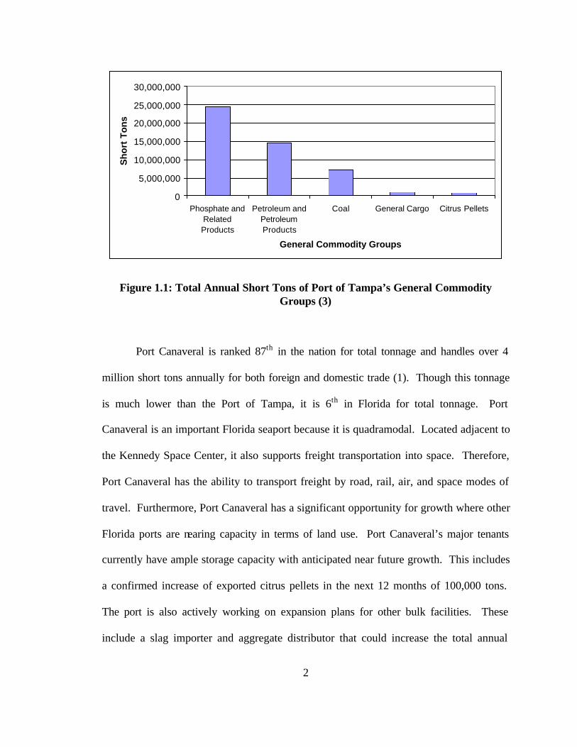
related products, which accounts for 50% of Tampa’s total annual tonnage. Figure 1.1 is
a breakdown of Tampa’s freight activity by general commodity groups.
2
0
5,000,000
10,000,000
15,000,000
20,000,000
25,000,000
30,000,000
Phosphate andRelatedProducts
Petroleum andPetroleumProducts
Coal General Cargo Citrus Pellets
General Commodity Groups
Sh
ort
To
ns
Figure 1.1: Total Annual Short Tons of Port of Tampa’s General Commodity Groups (3)
Port Canaveral is ranked 87th in the nation for total tonnage and handles over 4
million short tons annually for both foreign and domestic trade (1). Though this tonnage
is much lower than the Port of Tampa, it is 6th in Florida for total tonnage. Port
Canaveral is an important Florida seaport because it is quadramodal. Located adjacent to
the Kennedy Space Center, it also supports freight transportation into space. Therefore,
Port Canaveral has the ability to transport freight by road, rail, air, and space modes of
travel. Furthermore, Port Canaveral has a significant opportunity for growth where other
Florida ports are nearing capacity in terms of land use. Port Canaveral’s major tenants
currently have ample storage capacity with anticipated near future growth. This includes
a confirmed increase of exported citrus pellets in the next 12 months of 100,000 tons.
The port is also actively working on expansion plans for other bulk facilities. These
include a slag importer and aggregate distributor that could increase the total annual

3
tonnage of the port by up to 4 million. Figure 1.2 is a breakdown of Canaveral’s freight
activity by general commodity groups.
1,461,423
475,160
16,277 34,513 29,315147,745
672,308
124,004150,942
0
200,000
400,000
600,000
800,000
1,000,000
1,200,000
1,400,000
1,600,000
Petro
leum
Cemen
t
Newspr
int Salt
Lumber
Aggre
gate
Rebar/
Granite Citru
s
Genera
l Carg
o
Commodity
To
nn
age
Figure 1.2: Total Annual Short Tons of Port Canaveral’s General Commodity Groups (3)
1.1 Truck Traffic Generated by Seaport Freight Activity
Seaports are significant generators of heavy truck traffic. This is directly attributed to
the vessel freight activity. Each Florida seaport can be considered a high intermodal
traffic generator because at least two modes of transportation are utilized to move cargo
at the ports. The highest intermodal traffic is between the vessels and the heavy trucks
traveling on Florida’s highways.

4
From field data collected between years 2000 and 2001, Florida’s major seaports
generate over 10,000 daily heavy truck trips per direction (inbound or outbound) due to
port freight activity. These trucks travel on Florida’s highway network that connects to
these ports. Therefore, it is important to determine which routes the truck drivers use.
Defining the road network adjacent to Florida’s seaports is useful in examining existing
traffic operations, incident management, future planning and can also be utilized with
various intelligent transportation systems (ITS) applications including Advanced Traveler
Information Systems (ATIS).
In order to utilize a defined network adequately, a methodology for developing a
route assignment model of the road network adjacent to a Florida seaport must be
developed. This allows the transportation engineer or planner the ability to examine and
determine what impacts the seaports are having or will have on the local network traffic.
This methodology is also desired to be transferable to other ports as well. To produce an
accurate model, a computer simulation package can be utilized.
To develop a methodology for this network modeling approach, Florida’s largest
seaport, the Port of Tampa, was selected. In year 2000 the Port of Tampa generated over
4,000 daily truck trips per direction from freight activity. To test the transferability of the
methodology, Port Canaveral, the Port of Tampa’s eastern seaboard neighboring port,
was selected. Both ports are centrally located on each of Florida’s longitudinal coasts.

5
2. LITERATURE REVIEW
In 1996 M.G.H. Bell and S. Grosso, University of Newcastle, applied the Path
Flow Estimator (PFE) as a stochastic user equilibrium traffic assignment method (4).
This provides unique estimates of path flows and travel times from traffic counts and
prior origin-destination data. The program was written in the “C” computer language.
The PFE theory considers a two-path network. The relationship between the cost
of the two paths and the share of the traffic attracted was determined by the least cost of a
link. The input values to the program were links, nodes (intersections), geometric
features, traffic counts, signal times and the available origin-destination (O-D) data. The
output was path flows and path travel times. The algorithm used in the PFE is iterative,
with an inner and outer loop. The path flows were sequentially scaled in the inner loop
so the constraints are fulfilled. For the outer loop, link costs were calculated and least
cost paths are sought.
The O-D matrix used can be considered as a group of constraints for each
iteration. PFE was used in two cities, Turin and Toulouse. It produced poor results in the
first city and good results in the latter. The measure of effectiveness was the Mean
Absolute Error (MAE). The accepted threshold was within 20% of the measured values
for each link.
PFE cannot be used in multi-modal networks. It does not consider different
vehicle types (i.e. heavy trucks, passenger cars), driver behaviors or car following
theories. The program also does not assign heavy trucks on a road network.

6
In 1998, R. Boning, G. Eisenbei, C. Gawron, S. Krau, R. Schrader, and P.
Wagner, ZPR from Koln, Germany, used microscopic simulation to solve the Dynamic
Traffic Assignment (DTA) problem (5). The research was conducted at a research center
in Koln, Germany. A comparison between static and dynamic traffic assignment was
done. The algorithm used in the simulation-based DTA works as follows: any traveler
has a set of routes (usually small) to choose from. Associated with the routes is a
probability to choose the traveler’s route. After assigning a route to any of the travelers
according to these probabilities, a simulation was carried out that leads to the actual
travel times. These actual travel times were used to shift the probabilities towards shorter
routes. Convergence was reached when these probabilities no longer change.
Complication was created because the route choice depends on the traffic conditions
which itself depend on the routes chosen. Therefore, the double iteration loop shown in
Figure 2.1 was needed.

7
Micro-simulation
Convergence? No
Routes
Travel Times
Travel Times Destinations
Destinations Router
Yes
Micro-simulation
Convergence? No
Routes
Travel Times
Travel Times Destinations
Destinations Router
Yes
Figure 2.1: The Double Iteration Loop (5)
Finding the routes through a given network, the so-called DTA, can be
mathematically formulated as an optimization problem with linear constraints. Using the
assumption that individual travelers try to find the shortest or least cost route through a
network, the problem was complicated because the travel times on a link depended on the
number of cars on that link. The paper concluded that when dealing with a dynamic
problem, the classic approach using time independent flows was no longer suitable,
because a number of additional dynamic constraints have to be taken into account. To
name only the most important ones: 1-spillback phenomena have to be described and 2-
the FIFO (First In First Out) condition has to be fulfilled.
A simulation was performed on a German freeway network and urban road
network with a static and dynamic O-D matrix provided by the DLR (Department of

8
Transportation in Germany). It was concluded that the differences found were small.
Differences between static and dynamic assignment only showed up when the demand
exceeded the capacity during the rush hour and the link travel times could not be
adequately described as a static function of the link flows. All travel modes other than
passenger cars such as public transportation vehicles, trucks or bicycles were not
included in this research. It is not certain what the performance of this simulation
methodology would be for application to heavy trucks without extensive further research.
In 1999, Khaled F. Abdelghany and Hani S. Mahmassani have presented a
Dynamic Trip Assignment (DTA) simulation model for urban inter-modal transportation
networks (6). The model considered different travel modes such as private cars, buses,
metro/subway and High Occupancy Vehicles (HOV). The model captured the interaction
between mode choice and traffic assignment under different information provision
strategies. It implemented a multi-objective assignment procedure in which travelers
choose their modes and routes based on a range of evaluation criteria. The model
assumed a stochastically diverse set of travelers in terms of their relevant choice criteria
and access and response to the supplied information.
In this research the vehicular traffic flow simulation logic in DYNASMART was
adapted to represent interactions among transit vehicles and automobiles. This
simulation component is a time-based simulation, which moves individual vehicles along
links according to local speeds determined consistently with macroscopic traffic stream
models (i.e. a speed-density relation, a modified form of Greenshields, was used in this
implementation). The number of vehicles on each link was calculated using conservation
principles; numbers in each class of vehicles in the traffic mix were kept separate.

9
Consistently with the macroscopic logic for modeling vehicle interactions, average
passenger car equivalent factors were used to convert each vehicle type to the equivalent
passenger car units. The resulting equivalent-car concentration was then calculated for
each link, and used to estimate the corresponding speed through the speed-density
relation. These speeds, updated continually to reflect prevailing conditions, determine
vehicular movement on that link. This research however did not include any field data to
calibrate or validate the developed model. Furthermore, the developed model did not
include truck traffic as a major factor in the traffic assignment. Truck traffic may have a
significant influence on the overall study area’s operational performance because it
included an interstate highway (I-35W). Typically interstates may have a truck volume
high enough to influence the traffic operations. Due to these observations, this developed
model may not be adequate to meet the required research objectives of the truck-seaport
study.
In 2000, Wang, Messmer, and Papgeorgiou presented METANET, a macroscopic
simulation program for freeway networks (7). METANET was extended to include user-
optimal dynamic traffic assignment (DTA). A derivative of METANET called
METANET-DTA was developed which employs iterative algorithms for exact DTA.
DTA refers to distributing traffic demand with the same origin-destination (O-D) matrix
among alternative routes of a traffic network for all time periods, so that some optimality
principles are satisfied. Here, the origin refers not only to origins of a network, but also
to internal bifurcation nodes. Based on different optimality principles adopted, DTA is
generally classified as user-optimal DTA.

10
This research studied a complex network of freeways and did not include any of
the urban arterials. There were no signalized intersections in the study because of the
nature of the simulation program (Macroscopic simulation). METANET-DTA can not be
used in truck simulation for a small road network because it does not have the required
features to code signalized intersections or account for truck traffic.
In 1998, Peter Vovsha and Shlomo Bekhor, have investigated three models for
traffic assignment and route choice (8). The research included three mathematical
models to solve the traffic assignment problem. These models were Deterministic User
Equilibrium, Stochastic User Equilibrium by Multinomial Logit Route Choice, and
Stochastic User Equilibrium by the Link-Nested Logit Model. Numerical examples for
these three models were documented as well. It was concluded that the Link-Nested
model can be incorporated into a stochastic user equilibrium framework. The numerical
examples also showed the clear advantage of the Link-Nested Logit Model over the
deterministic and the Multinomial Logit Models with respect to trip loading quality.
However, the computational efficiency of the loading procedure was hampered by the
multiple repetition of the shortest path searching for each O-D.
This research did not include any collected field data for calibration or validation.
Moreover, it did no t account for the traffic composition or the special generators (ports,
shopping malls, etc.) as major factors affecting the solution of the traffic assignment
problem. Therefore, this approach was not applicable for this study.
In 2000 Loren Bloomberg and Jim Dale compared the VISSIM and CORSIM
traffic simulation models for a congested network (9). The ir paper included modeling of
SR 519 using VISSIM and CORSIM. It was concluded that the simulation approach was

11
effective for quantifying the benefits and limitations of different alternatives. The results
proved the consistency and reasonableness of the simulation tools, and provided the
authors with confidence about the results. The study also included sensitivity analysis. It
was also concluded that both models are appropriate for congested arterial street
conditions.
The research by Bloomberg and Dale provided evidence that a microscopic
simulation approach can be successfully executed for modeling congested networks. The
paper did not include the traffic assignment application in CORSIM or VISSIM
evaluations. An extension of this modeling approach using two simulation models will
be applied for solving the truck route assignment problem at Florida Seaports.
12
3. METHODOLOGY
The methodology is an application of simulation techniques for solving a dynamic
traffic assignment problem. Two different micro simulation packages were investigated
for assigning the truck volumes generated by the Port of Tampa on the adjacent road
network and consequently on the interstate highways (I-4, I-75 & I-275) in the port's
vicinity. CORSIM version 5.0 and VISSIM version 3.5 were the two simulation
packages investigated. The developed methodology consisted of the following steps:
1. Examine road network and conclude a network definition. The first step is to
examine the road network by making field observations, reviewing general traffic
information, and compiling data that was previously collected at the port's
entrances and exits in Phase II of this study. Also, interviews are conducted with
port personnel and trucking companies who are familiar with the port's operation.
This provides more details on the actual routes traveled by trucks generated from
port freight activity.
2. Data collection and analysis. Data related to traffic volumes of turning
movements, geometric features, type of control at intersections and signal timing
data for all links and nodes of the proposed network are collected. Selection of
data sources was prioritized to quality, availability, and feasibility. Field traffic
counts for certain links were collected on the road network to calibrate and
validate the proposed models. Traffic counts on these selected links were
compared with the traffic volumes obtained from the simulation model’s output.
The data was entered into a database for model development and validation.
13
3. Network Coding. All proposed network links and nodes were coded in the
simulation model. The relevant geometric, existing control devices at
intersections and traffic features (traffic composition and signal timing) were
included.
4. Model Calibration. Conduct several runs using an estimated Origin -Destination
(O-D) matrix and adjust these matrix volumes in an iterative process to conclude
with the best O-D that provides minimum error between field and simulated
volumes of the selected links.
5. Model Validation. The model must be validated in order to assure that it
replicates the actual system. This was accomplished by entering truck volume
data (leaving and entering the port) not used during the model development
process. Then, the model predicted truck volumes on the selected links were
compared with the actual volumes using several statistical tests.
6. Conclusions. Interpret the results to establish conclusions and make
recommendations for future analysis.
7. Forecasting. Execute the best model to determine the truck route assignment for
a short term (five year) forecast.
3.1 Background of Study Sites
3.1.1 Port of Tampa
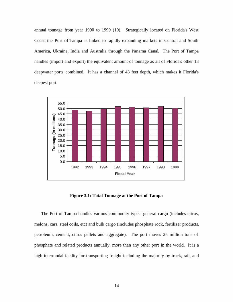
The Port of Tampa boasts some of the highest rated international and domestic
shipping facilities in the nation in terms of overall tonnage. Figure 3.1 shows the port’s
14
annual tonnage from year 1990 to 1999 (10). Strategically located on Florida's West
Coast, the Port of Tampa is linked to rapidly expanding markets in Central and South
America, Ukraine, India and Australia through the Panama Canal. The Port of Tampa
handles (import and export) the equivalent amount of tonnage as all of Florida's other 13
deepwater ports combined. It has a channel of 43 feet depth, which makes it Florida's
deepest port.
0.05.0
10.015.020.025.030.035.040.045.050.055.0
1992 1993 1994 1995 1996 1997 1998 1999
Fiscal Year
To
nn
age
(in
mill
ion
s)
Figure 3.1: Total Tonnage at the Port of Tampa
The Port of Tampa handles various commodity types: general cargo (includes citrus,
melons, cars, steel coils, etc) and bulk cargo (includes phosphate rock, fertilizer products,
petroleum, cement, citrus pellets and aggregate). The port moves 25 million tons of
phosphate and related products annually, more than any other port in the world. It is a
high intermodal facility for transporting freight including the majority by truck, rail, and

15
pipeline. It is also a major cruise port in Florida. A list of the site-specific information
for this port is:
• Three main freight terminal locations/Five main access roads
o Hookers Point (20th Street, 22nd Street, Causeway Blvd.)
o Port Sutton (Port Sutton Rd)
o Pendola Point (Pendola Point Rd)
• Rail activity present
• Significant petroleum imports in terms of volume
• Insignificant containerized imports/exports in terms of volume. The activity is
minimal especially compared to the bulk imports/exports.
• Significant bulk exports, including phosphate products and citrus pellets that are
very frequent and in high volumes.
A well-established port with high freight tonnage movement like the Port of Tampa is
expected to generate high heavy truck movements around the port and on the major
highways in its vicinity.
3.1.2 Port Canaveral
Port Canaveral is located to the East of Central Florida. It has two freight
terminals located on port property, a north terminal and south terminal. Access to each of
the terminals is independent. SR 401 is used for accessing the North Terminal and
George King Boulevard provides access to the South Terminal piers. As of year 2000,
Port Canaveral is reaching 5 million tons of total imports and exports. Figure 3.2 shows

16
the import and export trend in tonnage for the port over the last 7 years. Some of the
more significant imported commodities are petroleum, cement, newsprint, salt, lumber,
slate, granulated sand, drywall, rebar, and granite. Significant exports are concentrate,
juice, citrus, cars/trucks, and general cargo.
0
500,000
1,000,000
1,500,000
2,000,000
2,500,000
3,000,000
3,500,000
2000 1999 1998 1997 1996 1995 1994Year
ton
nag
e
Imports Exports
Figure 3.2: Port Canaveral Annual Imported and Exported Tonnage
This is a unique port because of its proximity to the Kennedy Space Center. It has
virtually unlimited growth potential due to the possible future increase in space travel and
subsequently the necessity to provide an intermodal hub for transporting freight into
space. It is also a major cruise port in Florida. A list of the site-specific information for
this port is:
• Two main freight terminal locations/two main access roads
o North Terminal (SR 401)
o South Terminal (George King Blvd.)
• Significant petroleum imports

17
• High tonnage cargos (bulk commodities) but infrequent shipments
• Insignificant containerized freight traffic
• Seasonal freight activity (citrus products)
• High storage capacity with many industries utilizing the port as business
operations centers including Rinker Materials, Morton Salt, Continental Cement,
Coastal Fuels, Ambassador Services, Mid-Florida Freezer.
Port Canaveral generates daily truck traffic due mainly to the high bulk cargo handled
here.

18
4. MODELING
4.1 Develop Route Assignment Model
Recently, there have been many traffic simulation packages developed to simulate
a wide array of traffic operations. CORSIM and VISSIM are two examples of existing
traffic micro simulation software. This research explores these two simulation packages
to investigate their capabilities in truck traffic assignment and to compare the two
packages. CORSIM and VISSIM were used as the tools for solving the traffic
assignment problem for the Port of Tampa road network. The outcome of the developed
modeling methodology and desired simulation package will be applied to Port Canaveral
to test the transferability. The following sections will explain the steps conducted to
achieve these goals.
4.1.1 Port of Tampa Network Definition
A preliminary road network has been identified for the Port of Tampa using the
Microsoft Expedia Street 98 Program. The information obtained from the map program
was compared with data from the 1999 FDOT Traffic Information CD. Also, several
trips were made to the Port of Tampa to examine the road network through field
observations. A sample of these trip reports is provided in Appendix A.
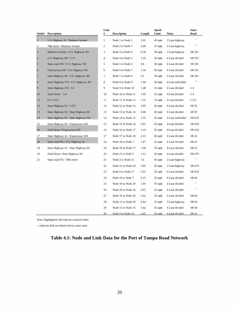
Table 4.1 shows the list of the network nodes and links with their geometric
features. The links listed in Table 4.1 were selected because they can accommodate high
truck volumes leaving and entering the Port of Tampa area according to the FDOT 1999

19
CD data. Figure 4.1 displays a diagram of the defined network. Most of the links are
interstate highways or state roads that have high capacity due to their geometric features.
The lower capacity roads were chosen because they link the major roads in the network
(i.e. Madison Avenue, SR 41, and SR 301). Major roads located in this area that are
considered main truck routes adjacent to the port are I-4, I-75, I-275, SR 41, SR 618, SR
92, and SR 60. Figure 4.2 shows a map of the Tampa network.
20
Node# DescriptionLink # Description Length
Speed Limit Notes
State Road
1 U.S. Highway 41 / Madison Avenue 1 Node 1 to Node 2 2.62 45 mph 2 Lane highway --
2 78th street / Madison Avenue 2 Node 2 to Node 3 2.69 35 mph 2 Lane highway --
3 Madison Avenue / U.S. Highway 301 3 Node 3 to Node 4 0.78 50 mph 2 Lane highway SR 301
4 U.S. Highway 301 / I-75 4 Node 4 to Node 5 1.45 50 mph 6 Lane divided SR 301
5 State road 676 / U.S. Highway 301 5 Node 5 to Node 6 0.6 50 mph 6 Lane divided SR 301
6 Expressway 618 / U.S. Highway 301 6 Node 6 to Node 7 1.34 50 mph 6 Lane divided SR 301
7 State Highway 60 / U.S. Highway 301 7 Node 7 to Node 8 2.3 50 mph 6 Lane divided SR 301
8 State Highway 574 / U.S. Highway 301 8 Node 8 to Node 9 1.44 50 mph 4 Lane undivided --
9 State Highway 574 / I-4 9 Node 9 to Node 10 1.48 55 mph 6 Lane divided I-4
10 22nd Street / I-4 10 Node 10 to Node 11 1.95 55 mph 4 Lane divided I-4
11 I-4 / I-275 11 Node 11 to Node 12 1.16 55 mph 4 Lane divided I-275
12 State Highway 92 / I-275 12 Node 12 to Node 13 3.85 45 mph 6 Lane divided SR 92
13 State Highway 92 / State Highway 60 13 Node 13 to Node 14 0.68 45 mph 6 Lane divided SR 92
14 State Highway 92 / State Highway 618 14 Node 14 to Node 15 3.35 65 mph 4 Lane undivided SR 618
15 State Highway 60 / Expressway 618 15 Node 15 to Node 16 5.61 65 mph 4 Lane divided SR 618
16 22nd Street / Expressway 618 16 Node 16 to Node 17 1.33 65 mph 4 Lane divided SR 618
17 State Highway 41 / Expressway 618 17 Node 17 to Node 18 2.15 65 mph 6 Lane divided SR 41
18 State road 676 / U.S. Highway 41 18 Node 18 to Node 1 1.87 55 mph 6 Lane divided SR 41
19 State Highway 41 / State Highway 60 19 Node 19 to Node 17 1.49 55 mph 6 Lane divided SR 41
20 22nd Street / State Highway 60 20 Node 21 to Node 5 1.12 45 mph 4 Lane divided SR 676
21 State road 676 / 78th street 21 Node 2 to Node 21 1.6 45 mph 2 Lane highway --
22 Node 21 to Node 18 3.85 45 mph 2 Lane highway SR 676
23 Node 6 to Node 17 2.91 55 mph 6 Lane divided SR 618
24 Node 19 to Node 7 0.15 35 mph 6 Lane divided SR 60
25 Node 10 to Node 20 1.05 55 mph 4 Lane divided --
26 Node 20 to Node 16 2.07 55 mph 6 Lane divided --
27 Node 19 to Node 20 3.42 55 mph 6 Lane divided SR 60
28 Node 15 to Node 20 0.64 35 mph 2 Lane highway SR 60
29 Node 13 to Node 15 3.42 55 mph 6 Lane divided SR 60
30 Node 9 to Node 19 3.42 55 mph 6 Lane divided SR 41
Note: Highlighted cells indicate external nodes.
-- indicates link not identivied as a state road.
Table 4.1: Node and Link Data for the Port of Tampa Road Network

21
Figure 4.1: Port of Tampa Network Diagram
8
24
236
7
22
12118 4
32
5
17
16
1413
2912
11
10 9
25 30
15
28 27
Node 9
Node 4
Node 1
Node 18
Node 16
Node 10Node 11
Node 12
Node 14
Node 7
Node 8
20
Node 13 Node 6
Node 5
Node 3
Hooker’sPoint
Pendola Point
Port Sutton
Figure 4.2: Road Network for the Port of Tampa O-D Matrix
(Microsoft Expedia Street 98 CD)

22
Trips were made to the port area for investigating the defined network. All nodes
were checked to determine if there were significant changes in the geometric features on
the links from the FDOT data. Also during these trips, interviews were conducted with
Port of Tampa personnel and trucking companies who are familiar with the port's freight
operations and possible truck routes. It was indicated from interviews with trucking
companies that most of the trucks leaving the port from Nodes 1 and 18 are heading
towards east (Bone Valley). It was also indicated that most of the trucks leaving the Port
from Node 16 are heading towards North (I-4, I-275). See Figure 4.2 for the node
locations on the Tampa road network.
The final defined road network was a cordon of about a 6.00-mile radius that
included 30 links and 21 nodes, see Figure 4.1. A node is defined as an intersection or an
interchange and links are the road segments that connect any two nodes. Figure 4.2
shows the network has 8 freeway links and 22 links on either state roads or urban streets.
For a description of the individual links, refer to Table 4.1. Three of the 8 freeway links
are on a toll road (SR 618). The network is bounded by SR 301 to the East, I-4 & I-275
to the north, and I-75 is located south east of the network. The nodes identified on the
map in Figure 4.2 are external nodes of the network. External nodes are the origin-
destination points for the network and make up the Origin-Destination (O-D) matrix used
as input to the computer simulation models. These can be a special generator such as a
port, an intersection, interchange, or a termination point on a network link that extends
outside the selected network boundary.

23
4.1.2 Port of Tampa Network Data Collection
As mentioned earlier, the required data for coding, calibrating, and validating any
simulation model are:
• Turning movements at each intersection and/or interchange,
• Geometric features,
• Type of control at an intersection,
• Signal timing and
• Traffic volumes on each link.
The City of Tampa and Hillsborough County provided signal-timing data for all
the signalized intersections. A sample of this data is shown in Appendix B. Geometric
features of the network and signal timing data for all network locations were not
available. The missing information about the network geometry and type of control at
intersections on the network was obtained during the field trips to the Port of Tampa’s
surrounding road network. During these trips, all of the proposed network links were
driven on to record more data. Speed limits and geometric features were recorded and
verified for each network link.
FDOT was contacted to obtain any available truck volumes for the network links.
A hard copy of relevant data records from FDOT District 7 was obtained. Table 4.2
includes the data necessary for coding the network that was received from FDOT for the
Port of Tampa links on the road network. It also includes the link number, station
number according to FDOT’s numbering system, Average Annual Daily Traffic (AADT),
K factor that is the ratio between the peak hour volume and the daily volume, directional
factor (D), and the percent of trucks (T). This data was used to update the data originally

24
recorded from the 1999 FDOT traffic data CD. Due to the fact that, I-275 is the only
interstate highway that is directly connected to Hookers Point (through I-4 at Node 10)
and is north, I-275 provides service to most of the freight trucks traveling on routes north
of Hookers Point (Node 16). This volume of trucks on I-275 (Link 11) is displayed in
Table 4.2. However, freight trucks traveling on routes north of Pendola Point through
Madison Avenue (Link 1) can use I-75 (at Node 4).
Link Number Station Number Source Age of Data AADT K D T
Truck Volume
123 0044 District 7 AADT Mar-00 23500 10.37 54.55 10.68 25104 5259 District 7 AADT Mar-00 17000 10.37 54.55 8.32 14145 5260 District 7 AADT Mar-00 16000 10.37 54.55 7.88 12616 5325 District 7 AADT Mar-00 16500 10.37 54.55 6.81 11247 5326 District 7 AADT Mar-00 17500 10.37 54.55 8.51 14898
9 2026 & 2027 District 7 AADT Mar-00 64000 9.74 54.48 13.42 858910 2028 District 7 AADT Mar-00 70000 9.74 54.48 10.93 765111 2015 & 2016 District 7 AADT Mar-00 84000 9.74 54.48 10.21 857612 5055 District 7 AADT Mar-00 28000 10.37 54.55 5.01 140313 5052 District 7 AADT Mar-00 18500 10.37 54.55 8.18 151314 5244 District 7 AADT Mar-00 11000 10.37 54.55 8.51 93615 5277 District 7 AADT Mar-00 23500 10.37 54.55 8.05 189216 5264 District 7 AADT Mar-00 25000 10.37 54.55 3.63 90817 0003 District 7 AADT Mar-00 11000 10.37 54.55 11.6 127618 5258 District 7 AADT Mar-00 9900 10.37 54.55 11.71 1159
19 5104 District 7 AADT Mar-00 16500 10.37 54.55 10.22 168620, 22 0030 District 7 AADT Mar-00 9500 10.37 54.55 6.86 6522123 5266 District 7 AADT Mar-00 21000 10.37 54.55 3.1 65124 5123 District 7 AADT Mar-00 19500 10.37 54.55 7.68 149825 5300 & 5305 District 7 AADT Mar-00 16000 10.37 54.16 16.72 267526 5299 & 5300 District 7 AADT Mar-00 11500 10.37 51.11 16.72 192327 5126 District 7 AADT Mar-00 14000 10.37 54.55 7.66 107228 5131 District 7 AADT Mar-00 6700 10.37 54.55 6.01 403
29 0029 District 7 AADT Mar-00 15500 10.37 54.55 7.21 111830 5104 District 7 AADT Mar-00 16500 10.37 54.55 10.22 1686Shaded cells indicate the missing link data
Table 4.2: FDOT Link Data for the Port of Tampa Road Network

25
Turning movement volumes for the peak hour were also included in the FDOT
traffic operations data. Turning movements were provided for every fifteen minutes of
the morning and evening peak periods. Once the available port network data was
examined, any remaining traffic volumes necessary for completing the development of
the route assignment model were obtained from actual field data collection.
4.1.3 Port of Tampa Field Traffic Data Collection: Freight Terminals
Figure 4.3 shows a layout of the port area. The blue stars indicate the five data
collection locations for the truck counts at the freight terminals.

26
Figure 4.3: Port of Tampa Area Map
Traffic counts that were previously collected during Phase II of this study for the
Port of Tampa were utilized in Phase III also. Hourly volumes by vehicle class have
been collected for the five sites at the Port of Tampa in Phase II of this Truck Study.
Three sites are at Hookers Point (22nd Street, 20th Street and Causeway Boulevard) and
Port Sutton/Pendola Point
Hooker’s Point

27
two sites are at Pendola Point (Port Sutton Road and Pendola Point Road). Up to 168
days of truck counts were collected at these sites. The total number of days at each site is
shown Table 4.3. This data provides truck counts for Nodes 1, 16 and 18. Figure 4.2
displays the road network map with these nodes identified.
Location and Direction Number of Days
Pendola Point Road - Inbound 168
Pendola Point Road - Outbound 168
Port Sutton Road - Inbound 147
Port Sutton Road - Outbound 147
Causeway Boulevard - Inbound 120
Causeway Boulevard - Outbound 119
22nd Street - Inbound 134
22nd Street - Outbound 106
20th Street - Inbound 122
20th Street - Outbound 151 Table 4.3: Number of Days for Truck Counts Collected on the Port of Tampa’s
Access Roads during Phase II Study
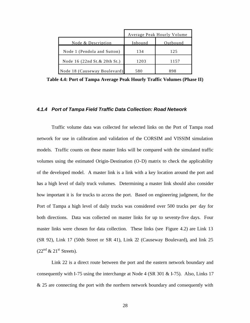
Peak hour traffic volumes collected from the field at the port's entrances and exits
have been compiled and summarized in Table 4.4. These entrances and exits are
represented on the network by Node 1 (Pendola Point and Port Sutton), Node 16 (22nd
Street and 20th Street), and Node 18 (Causeway Boulevard). The table shows the average
peak hour traffic volumes leaving and entering the Port of Tampa. The average peak
hour traffic volumes is the arithmetic mean of the peak hour volumes of up to 168 days of
data collected during Phase II of this project.
28
Node & Description Inbound Outbound
Node 1 (Pendola and Sutton) 134 125
Node 16 (22nd St.& 20th St.) 1203 1157
Node 18 (Causeway Boulevard) 580 898
Average Peak Hourly Volume
Table 4.4: Port of Tampa Average Peak Hourly Traffic Volumes (Phase II)
4.1.4 Port of Tampa Field Traffic Data Collection: Road Network
Traffic volume data was collected for selected links on the Port of Tampa road
network for use in calibration and validation of the CORSIM and VISSIM simulation
models. Traffic counts on these master links will be compared with the simulated traffic
volumes using the estimated Origin-Destination (O-D) matrix to check the applicability
of the developed model. A master link is a link with a key location around the port and
has a high level of daily truck volumes. Determining a master link should also consider
how important it is for trucks to access the port. Based on engineering judgment, for the
Port of Tampa a high level of daily trucks was considered over 500 trucks per day for
both directions. Data was collected on master links for up to seventy-five days. Four
master links were chosen for data collection. These links (see Figure 4.2) are Link 13
(SR 92), Link 17 (50th Street or SR 41), Link 22 (Causeway Boulevard), and link 25
(22nd & 21st Streets).
Link 22 is a direct route between the port and the eastern network boundary and
consequently with I-75 using the interchange at Node 4 (SR 301 & I-75). Also, Links 17
& 25 are connecting the port with the northern network boundary and consequently with

29
I-4 & I-275. Link 25 consists of two different one-way roads. These two roads are 21st
street, which carries the traffic from I-4 to the Port of Tampa, and 22nd street, which
carries the traffic from the Port of Tampa to I-4. Due to the fact that Link 29 goes
through downtown Tampa, no data collection was conducted on this link because it
carries virtually no port-generated trucks. The trucks would experience high delay if they
traveled through the downtown due to the high number of signalized intersections.
Traffic counts were also conducted at Node 9. Node 9 has been chosen because it
connects to Link 9 (part of I-4) that carries a high volume of trucks according to FDOT
data (see Table 4.2). Traffic can leave the network at Node 9 using two different roads.
The vehicles that are exiting Tampa network at Node 9 use I-4 or SR 41. From SR 41 to
the I-4 interchange, it is a two- lane bi-directional road. The I-4 interchange has on and
off ramps for both the eastbound and westbound directions. To capture trucks exiting the
Tampa network, data was collected north of the SR41/SR574 intersection on SR 41 and
the eastbound on-ramp for I-4. The total number of vehicles exiting the network at Node
9 is the summation of the number of vehicles exiting the defined network towards I-4 and
vehicles that are heading towards the northbound direction of SR 41.
The data was collected using Metrocount and Diamond Phoenix Traffic
Classifiers. The downloaded files were compiled and entered into a Microsoft Excel
spreadsheet. See Table 4.5 and Table 4.6 for an inventory of the daily truck counts for
each site. Seventy-five daily counts were collected. Some of these days have logged
data that displays inconsistent counts or no data was recorded due to equipment damage
or failure. Data was divided into two sets. The first set included two thirds of the
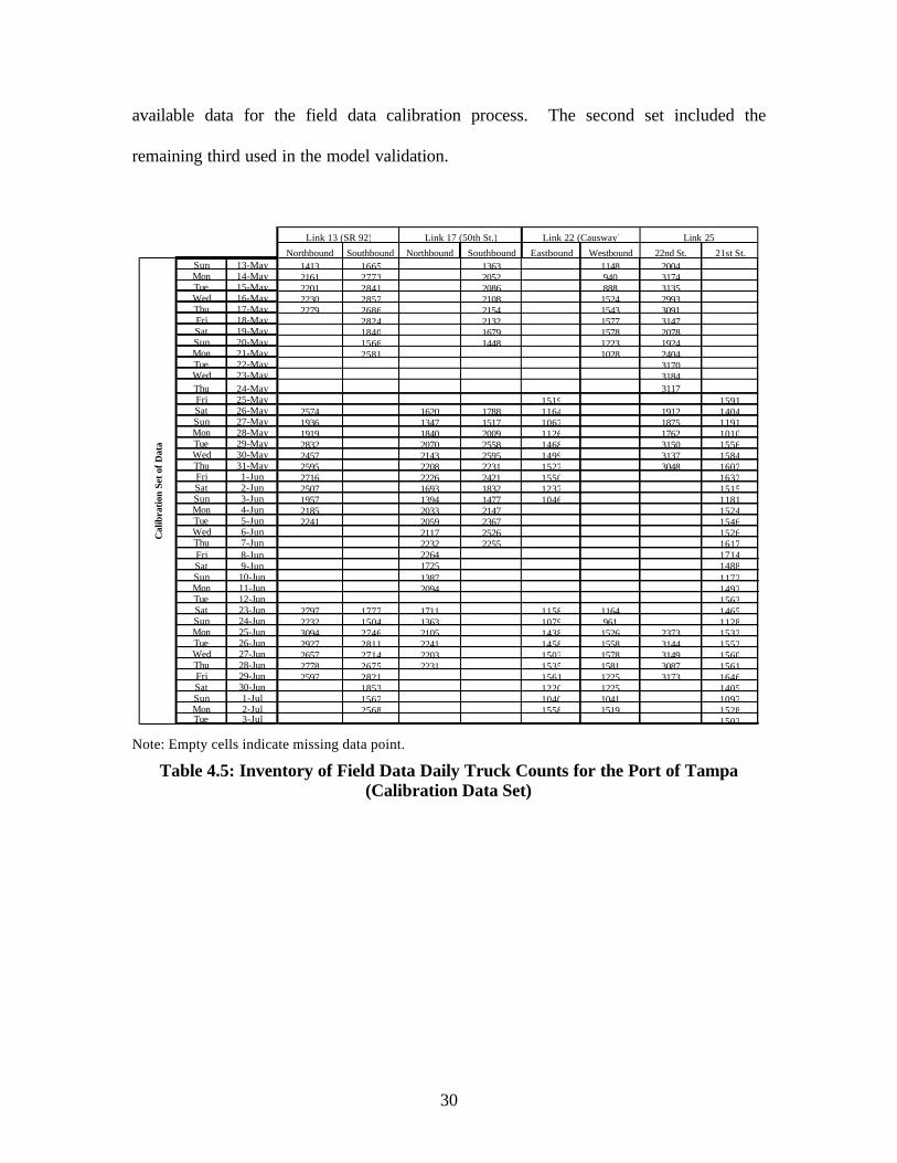
30
available data for the field data calibration process. The second set included the
remaining third used in the model validation.
Northbound Southbound Northbound Southbound Eastbound Westbound 22nd St. 21st St.Sun 13-May 1413 1665 1363 1148 2004Mon 14-May 2161 2773 2052 940 3174Tue 15-May 2201 2841 2086 888 3135Wed 16-May 2230 2857 2108 1524 2993Thu 17-May 2279 2686 2154 1543 3091Fri 18-May 2824 2132 1577 3147Sat 19-May 1840 1679 1578 2078Sun 20-May 1566 1448 1223 1924Mon 21-May 2581 1028 2404Tue 22-May 3170Wed 23-May 3184Thu 24-May 3117Fri 25-May 1519 1591Sat 26-May 2574 1620 1788 1164 1912 1404Sun 27-May 1936 1347 1517 1067 1875 1191Mon 28-May 1919 1840 2009 1126 1762 1010Tue 29-May 2832 2070 2558 1468 3150 1556Wed 30-May 2457 2143 2595 1499 3137 1584Thu 31-May 2595 2208 2231 1527 3048 1607Fri 1-Jun 2716 2226 2421 1550 1637Sat 2-Jun 2507 1693 1832 1237 1515Sun 3-Jun 1957 1394 1477 1046 1181Mon 4-Jun 2185 2033 2147 1524Tue 5-Jun 2241 2059 2367 1546Wed 6-Jun 2117 2526 1526Thu 7-Jun 2232 2255 1617Fri 8-Jun 2264 1714Sat 9-Jun 1725 1488Sun 10-Jun 1387 1172Mon 11-Jun 2094 1492Tue 12-Jun 1563Sat 23-Jun 2797 1777 1711 1158 1164 1465Sun 24-Jun 2232 1504 1363 1079 961 1128Mon 25-Jun 3094 2746 2105 1438 1526 2373 1532Tue 26-Jun 2927 2811 2241 1458 1558 3144 1552Wed 27-Jun 2657 2714 2203 1503 1578 3149 1560Thu 28-Jun 2778 2675 2231 1535 1581 3087 1561Fri 29-Jun 2597 2821 1561 1225 3173 1646Sat 30-Jun 1853 1220 1225 1405Sun 1-Jul 1567 1040 1041 1097Mon 2-Jul 2568 1558 1519 1528Tue 3-Jul 1502
Link 13 (SR 92) Link 17 (50th St.) Link 22 (Causway) Link 25
Cal
ibra
tion
Set o
f Dat
a
Note: Empty cells indicate missing data point.
Table 4.5: Inventory of Field Data Daily Truck Counts for the Port of Tampa (Calibration Data Set)

31
Northbound Southbound Northbound Southbound Eastbound Westbound 22nd St. 21st St. SR 41 I-4 on-Ramp
Thu 5-Jul 2779 2689 2244 2258 1554 1562 3075 1550 2131 369
Fri 6-Jul 2602 2784 2245 2454 1629 1646 3124 1648 2214 396
Sat 7-Jul 2506 1838 1670 1807 1303 1199 1961 1368 1572 245
Sun 8-Jul 2232 1504 1392 1452 1092 1012 1984 1121 1305 202
Mon 9-Jul 3094 2591 2034 2165 1596 1575 3095 1500 2128 370
Tue 10-Jul 2927 2806 2054 2386 1375 1464 3071 1510 2154 361
Wed 11-Jul 2657 2498 1519 1385 2919 1547 2065 369
Thu 12-Jul 2776 2268 1505 1439 1624 2165 387
Fri 13-Jul 2600 1572 1485 1683 2212 398
Sat 14-Jul 1298 1094 1438 1660 262
Sun 15-Jul 1079 961 1130 1332 202
Mon 16-Jul 3078 2526 1963 2186 1565 1509 2942 1478 2152 379
Tue 17-Jul 2898 2707 2433 2165 1643 1562 3099 1535 2156 359
Wed 18-Jul 2664 2724 2481 2351 1323 1646 3099 1584 2057 382
Thu 19-Jul 2783 2678 2512 25182 1121 1199 3029 1614 2152 379
Fri 20-Jul 2598 2762 2324 2268 1580 1012 3178 1654 2192 382
Sat 21-Jul 2388 1856 1704 1806 1298 1575 1936 1382 1654 257
Sun 22-Jul 2219 1564 1388 1452 1103 1464 2900 1083 1344 198
Mon 23-Jul 3080 2714 1996 2197 1603 1385 3117 1430 2160 360
Tue 24-Jul 2933 2675 2064 2379 1382 1439 1516
Wed 25-Jul 2821 1485 1532
Thu 26-Jul 2599 1094 1593
Fri 27-Jul 2856 961 1651
Sat 28-Jul 1419
Sun 29-Jul 1085
Mon 30-Jul 1458
Tue 31-Jul 1487
Wed 1-Aug 1224
Node 9Link 13 (SR 92) Link 17 (50th St.) Link 22 (Causway) Link 25
Val
idat
ion
Set o
f Dat
a
Note: Empty cells indicate missing data point.
Table 4.6: Inventory of Field Data Daily Truck Counts for the Port of Tampa (Validation Data Set)
The total number of vehicles (cars and trucks) was compiled for each of the data
collection points. Peak hour volumes were also extracted from the collected counts. The
peak hour volume for a day is the maximum hourly value during the 24-hour period.
This was found to be 5-6 PM. Table 4.7 shows a summary of the average daily and peak
hourly traffic volumes (cars and trucks) for the calibration set of days at each location.

32
Table 4.7: Summary of the Calibration Data Set for the Master Links at Port of Tampa Road Network
Peak hour volumes for each link were entered into the SPSS for Windows release
10.0.7 statistical analysis software. A preliminary analysis of the calibration data set was
performed using SPSS. A Scheffe's Statistical Test was conducted on the compiled data
to see if there was any significant difference between weekdays and weekends. Scheffe's
test identifies homogeneous subsets of means that are not different from each other. Pair-
wise multiple comparisons test the difference between each pair of means, and yield a
matrix where significantly different group means are indicated at a confidence level of
95%. See Appendix C for the SPSS analysis and results. An overview of the analysis for
each master link by direction is also included in this subsection.
75 days of counts collected on these master links were analyzed. The inconsistent
counts or missing records due to equipment damage or failure were excluded from the
calibration data sets selected for each link and direction. Table 4.5 and Table 4.6 can be
referenced for the dates data was included for each master link by direction.
For Link 13 (SR 92) northbound, the calibration data set included 23 days. From
Scheffe’s Statistical Test at the 95% confidence level, there was no significant difference
Location Direction Average Daily Counts Peak Hourly Volume
Northbound 12,159 1,094
Southbound 13,780 1,240
Northbound 10,688 802
Southbound 10,686 855Eastbound 7,181 646Westbound 6,350 572
22nd street (Link 25) Northbound 14,360 1,005
21st street (Link 25) Southbound 7559 718
I-92 (Link 13)
Causeway Boulevard (Link 22)
50th street (Link 17)

33
between truck counts on weekdays and weekends. See Appendix C for the SPSS analysis
results. Therefore, all available days were used to calculate the average vehicular
volumes. The average daily traffic (cars and trucks) volume northbound on Link 13 was
12,018 vehicles. The average peak hour traffic volume was 1,094 vph and the average
number of trucks for the peak hour was 164 trucks.
For Link 13 (SR 92) southbound, the calibration data set included 19 days. From
Scheffe’s Statistical Test at the 95% confidence level, there was a significant difference
between truck counts on weekdays and weekends. See Appendix C for the SPSS analysis
results. Therefore, the weekend days were excluded from the data used to calculate the
average vehicular volumes. The average daily traffic (cars and trucks) volume
southbound on Link 13 was 13,698 vehicles. The average peak hour traffic volume was
1,240 vph and the average number of trucks for the peak hour was 186 trucks.
For Link 17 (50th Street) northbound, the calibration data set included 23 days.
From Scheffe’s Statistical Test at the 95% confidence level, there was a significant
difference between truck counts on weekdays and weekends. See Appendix C for the
SPSS analysis results. Therefore, the weekend days were excluded from the data used to
calculate the average vehicular volumes. The average daily traffic (cars and trucks)
volume northbound on Link 17 was 10,688 vehicles. The average peak hour traffic
volume was 802 vph and the average number of trucks for the peak hour was 120 trucks.
For Link 17 (50th street) southbound, the calibration data set included 21 days.
From Scheffe’s Statistical Test at the 95% confidence level, there was no significant
difference between truck counts on weekdays and weekends. See Appendix C for the
SPSS analysis results. Therefore, all available days were used to calculate the average

34
vehicular volumes. The average daily traffic (cars and trucks) volume southbound on
Link 17 was 10,177 vehicles. The average peak hour traffic volume was 855 vph and the
average number of trucks for the peak hour was 128 trucks.
For Link 22 (Causeway Boulevard) eastbound, the calibration data set included 21
days. From Scheffe’s Statistical Test at the 95% confidence level, there was no
significant difference between truck counts on weekdays and Saturdays. However, there
was a significant difference between Sundays and all other days of the week. See
Appendix C for the SPSS analysis results. Therefore, all available days except Sundays
were used to calculate the average vehicular volumes. The average daily traffic (cars and
trucks) volume eastbound on Link 22 was 7,181 vehicles. The average peak hour traffic
volume was 646 vph and the average number of trucks for the peak hour was 97 trucks.
For Link 22 (Causeway Boulevard) westbound, the calibration data set included
20 days. From Scheffe’s Statistical Test at the 95% confidence level, there was no
significant difference between truck counts on weekdays and weekends. See Appendix C
for the SPSS analysis results. Therefore, all available days were used to calculate the
average vehicular volumes. The average daily traffic (cars and trucks) volume
westbound on Link 22 was 6,350 vehicles. The average peak hour traffic volume was
572 vph and the average number of trucks for the peak hour was 86 trucks.
For Link 25 (22nd Street) northbound, the calibration data set included 23 days.
From Scheffe’s Statistical Test at the 95% confidence level, there was a significant
difference between truck counts on weekdays and weekends. See Appendix C for the
SPSS analysis results. Therefore, the weekend days were excluded from the data used to
calculate the average vehicular volumes. The average daily traffic (cars and trucks)

35
volume northbound on Link 25 was 14,360 vehicles. The average peak hour traffic
volume was 1005 vph and the average number of trucks for the peak hour was 151
trucks.
For Link 25 (21st Street) southbound, the calibration data set included 30 days.
From Scheffe’s Statistical Test at the 95% confidence level, there was a significant
difference between truck counts on weekdays and weekends. See Appendix C for the
SPSS analysis results. Therefore, the weekend days were excluded from the data used to
calculate the average vehicular volumes. The average daily traffic (cars and trucks)
volume southbound on Link 25 was 7,559 vehicles. The average peak hour traffic
volume was 718 vph and the average number of trucks for the peak hour was 108 trucks.
Data was also collected at Node 9. This captured the volume of vehicles exiting
the network at this node. 13 days of data were used for the analysis at this node. These
counts were used in the validation of the network model. From Scheffe’s Statistical Test
at the 95% confidence level, there was a significant difference between truck counts on
weekdays and weekends. Therefore, the weekend days were excluded from the data used
to calculate the average vehicular volumes. The average daily traffic (cars and trucks)
volume exiting the network at this node is 20,484 vehicles. The average peak hour traffic
volume was 2,868 vph. These traffic volumes included counts at both the I-4 on-ramp
and the northbound direction of SR41.
4.1.5 Port of Tampa Data Collection: Vessel Freight Data
Three months of raw vessel freight data were used to determine the daily number
of trucks generated by the port’s freight activity that was used for the calibration and
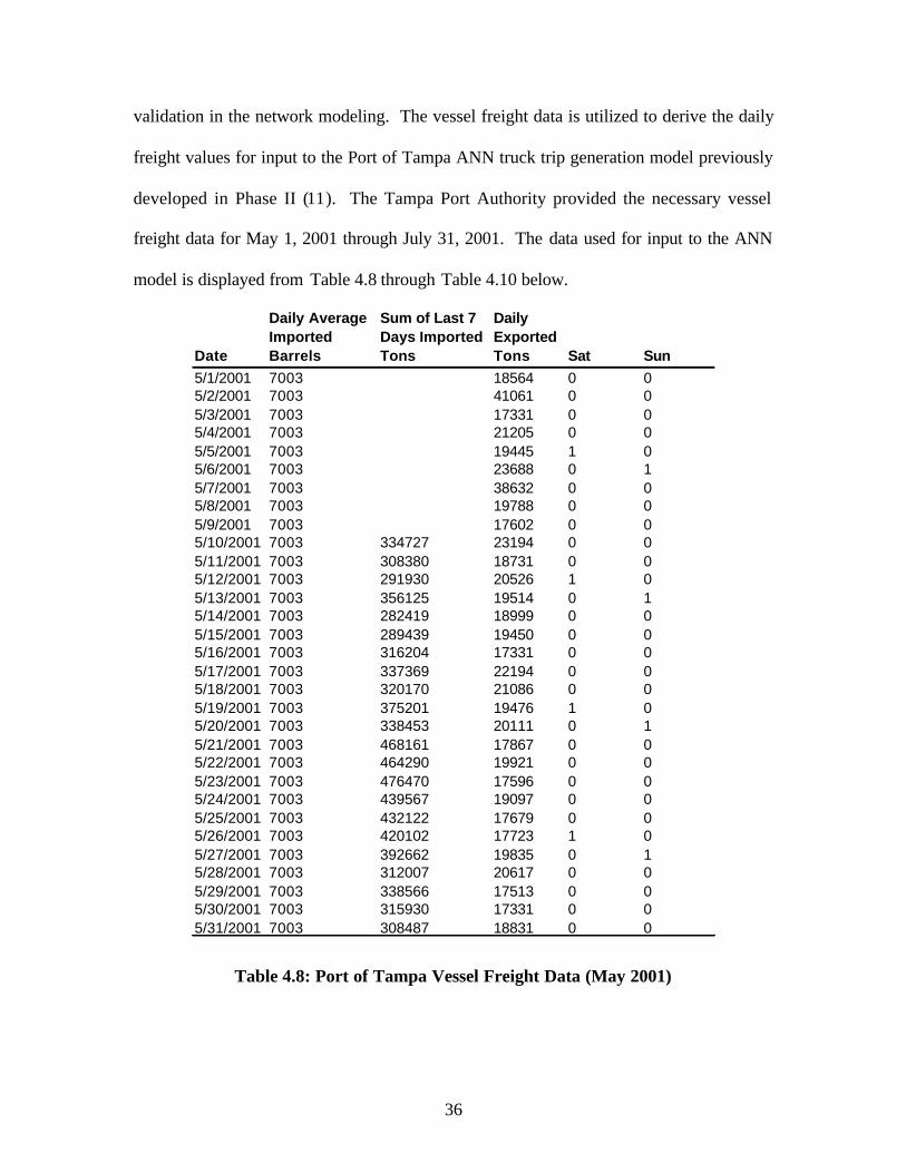
36
validation in the network modeling. The vessel freight data is utilized to derive the daily
freight values for input to the Port of Tampa ANN truck trip generation model previously
developed in Phase II (11). The Tampa Port Authority provided the necessary vessel
freight data for May 1, 2001 through July 31, 2001. The data used for input to the ANN
model is displayed from Table 4.8 through Table 4.10 below.
Date
Daily Average Imported Barrels
Sum of Last 7 Days Imported Tons
Daily Exported Tons Sat Sun
5/1/2001 7003 18564 0 05/2/2001 7003 41061 0 05/3/2001 7003 17331 0 05/4/2001 7003 21205 0 05/5/2001 7003 19445 1 05/6/2001 7003 23688 0 15/7/2001 7003 38632 0 05/8/2001 7003 19788 0 05/9/2001 7003 17602 0 05/10/2001 7003 334727 23194 0 05/11/2001 7003 308380 18731 0 05/12/2001 7003 291930 20526 1 05/13/2001 7003 356125 19514 0 15/14/2001 7003 282419 18999 0 05/15/2001 7003 289439 19450 0 05/16/2001 7003 316204 17331 0 05/17/2001 7003 337369 22194 0 05/18/2001 7003 320170 21086 0 05/19/2001 7003 375201 19476 1 05/20/2001 7003 338453 20111 0 15/21/2001 7003 468161 17867 0 05/22/2001 7003 464290 19921 0 05/23/2001 7003 476470 17596 0 05/24/2001 7003 439567 19097 0 05/25/2001 7003 432122 17679 0 05/26/2001 7003 420102 17723 1 05/27/2001 7003 392662 19835 0 15/28/2001 7003 312007 20617 0 05/29/2001 7003 338566 17513 0 05/30/2001 7003 315930 17331 0 05/31/2001 7003 308487 18831 0 0
Table 4.8: Port of Tampa Vessel Freight Data (May 2001)

37
Date
Daily Average Imported
Sum of Last 7 Days
Daily Exported Tons Sat Sun
6/1/2001 7107 274621 21198 0 06/2/2001 7107 235873 24764 1 06/3/2001 7107 296234 23852 0 16/4/2001 7107 290962 23406 0 06/5/2001 7107 296162 19772 0 06/6/2001 7107 286681 27972 0 06/7/2001 7107 302585 21690 0 06/8/2001 7107 356669 20918 0 06/9/2001 7107 390947 19772 1 06/10/2001 7107 409591 25098 0 16/11/2001 7107 399801 24449 0 06/12/2001 7107 418451 21586 0 06/13/2001 7107 404085 21127 0 06/14/2001 7107 413022 19772 0 06/15/2001 7107 372563 24284 0 06/16/2001 7107 372160 22747 1 06/17/2001 7107 367315 23829 0 16/18/2001 7107 371896 19772 0 06/19/2001 7107 381628 23489 0 06/20/2001 7107 355891 20027 0 06/21/2001 7107 357256 22467 0 06/22/2001 7107 381615 26097 0 06/23/2001 7107 418889 20240 1 06/24/2001 7107 406074 22518 0 16/25/2001 7107 377606 22229 0 06/26/2001 7107 315063 53157 0 06/27/2001 7107 330687 21181 0 06/28/2001 7107 317786 19772 0 06/29/2001 7107 309057 21616 0 06/30/2001 7107 239543 19772 1 0
Table 4.9: Port of Tampa Vessel Freight Data (June 2001)

38
Date
Daily Average Imported
Sum of Last 7 Days
Daily Exported Tons Sat Sun
7/1/2001 6972 197154 26391 0 17/2/2001 6972 286324 23260 0 07/3/2001 6972 320197 23234 0 07/4/2001 6972 419477 23406 0 07/5/2001 6972 480701 25122 0 07/6/2001 6972 437527 23934 0 07/7/2001 6972 432876 26434 1 07/8/2001 6972 469714 25808 0 17/9/2001 6972 407473 25120 0 07/10/2001 6972 384559 23234 0 07/11/2001 6972 327581 23234 0 07/12/2001 6972 297143 24476 0 07/13/2001 6972 334903 23560 0 07/14/2001 6972 373802 25129 1 07/15/2001 6972 368287 64801 0 17/16/2001 6972 428630 26058 0 07/17/2001 6972 393386 23251 0 07/18/2001 6972 365711 23566 0 07/19/2001 6972 374954 25206 0 07/20/2001 6972 428874 23234 0 07/21/2001 6972 409519 23736 1 07/22/2001 6972 479318 25866 0 17/23/2001 6972 407741 25739 0 07/24/2001 6972 494448 51752 0 07/25/2001 6972 521712 62538 0 07/26/2001 6972 317786 23234 0 07/27/2001 6972 309057 23234 0 07/28/2001 6972 239543 23234 1 07/29/2001 6972 197154 25848 0 17/30/2001 6972 286324 0 07/31/2001 6972 320197 0 0
Table 4.10: Port of Tampa Vessel Freight Data (July 2001)
4.1.6 Port of Tampa Network Coding: CORSIM
A corridor microscopic simulation model, known as CORSIM, was used to
complete the task of truck assignment on the defined road network adjacent to the Port of
Tampa. CORSIM is a microscopic simulation model with a module called TA (Traffic
Assignment) which converts an Origin-Destination (O-D) trip table into an actual

39
network loading for processing by CORSIM. The model then evaluates demand
responses to operational changes. Operational changes may include incidents or signal
timing changes. TA uses two optimization techniques in CORSIM. These techniques are
the user's optimal assignment and system's optimal assignment. The model applies the
shortest path algorithm to assign the volumes on the network links. The input data
required for the model are traffic composition, geometric features of the network, signal
timing, and an O-D table. CORSIM has two available impedance functions to evaluate
travel time on a path-link (group of links on a truck route). The first impedance function
(FHWA) is shown below.
Where
T = Mean travel time on the path- link T0 = Free-flow (zero volume) travel time on the path-link V = Volume on the path- link C = Capacity of the path- link a = 0.60, b = 4
The second is the Modified Davidson's impedance function as follows:
( )
−
+=VS
VaTT *1*0
If V < b * S
Or
( )( )
( )[ ]2001*
*1
*1*bS
bSVTa
bb
aTT−
−+
−
+=
If V > b * S
+=
b
CV
aTT *1*0
40
Where
T = Mean travel time on the path- link T0 = Free-flow (zero volume) travel time on the path-link V = Volume on the path- link C = Capacity of the path- link S = Path- link saturation rate = 100(C/R) R = Ratio of Capacity to Saturation rate in % a = 0.40, b = 0.80
The travel time on a path link includes the time required to traverse the geometric
link and the time required at its downstream intersection to perform the desired turning
movement. The FHWA impedance function was chosen because it is recommended by
the CORSIM manual (l2).
CORSIM has two modules for coding the road network. The first module is
NETSIM (Surface Street NETwork traffic flow micro SIMulation model). NETSIM is
the module used to code arterial roads in the network. The other module is FRESIM
(FREeway traffic flow micro SIMulation model). CORSIM Traffic Assignment (TA)
does not have the ability to perform traffic assignment to a road network that consists of
freeways and arterials (city streets) simultaneously. Therefore, links on freeways (Link
numbers 9, 10, 11, 14, 15, 16 & 23) were modeled using the NETSIM module. A
relatively high free flow speed (55 mph) was assigned to those links. The higher free
flow speed was assigned to links on freeways to match real- life conditions. All network
links and nodes at the Port of Tampa were coded in NETSIM. All the geometric data for
each link and node (i.e. number of lanes and intersection configurations) were considered
during the coding. Signal timing and any existing control devices at intersections (nodes)
were incorporated in the model. Initial O-D volumes for the network were estimated.
These are the distribution percentages of trucks leaving the port (Nout) or coming to the
41
port (Nin) on the proposed network based on the information obtained from interviews
with local freight operations personnel. These percentages refer to the percent of total
trucks for the external nodes of the network that are originating from or destined to the
nodes associated directly with the port.
The network coding can be checked visually using the TRAFVU module.
TRAFVU is a CORSIM module used for viewing the coded network and performing
animation of the network model. A preliminary truck assignment model run was
performed on the coded Tampa road network. The network included all the links and
nodes defined before for the Port of Tampa road network. Truck assignment was
performed by CORSIM and the model run did not produce any errors. A snapshot of the
animation obtained from TRAFVU module is shown in Figure 4.4. The snapshot is for
the intersection of SR 676 and US 41, one of the five Tampa Port exits located on the
western side of this intersection. This run was performed to check the applicability of
solving the truck assignment problem.

42
Figure 4.4: Snapshot of the Animation for the Simulated Intersection of State Road 676 and US 41
4.1.7 Port of Tampa Network Coding: VISSIM
Another simulation package known as VISSIM, (version 3.5) was investigated for
assignment of trucks on the proposed network. VISSIM is a microscopic simulation
model, which has a Dynamic Assignment (DA) module. Nodes and edges have to be
defined for the network of interest. Nodes represent intersections or junctions and edges
represent link sequences. A sequence of edges on the modeled road network between the
starting and the ending point is called a route. Every driver selects a specific route at the
departure time. These route choice decisions of all drivers add up to a dynamic
assignment of the given transport demand, thus determining the traffic volumes on the

43
road network. These traffic volumes affect travel times on the network. The volumes
and travel times are not constant during the simulation period and therefore the fastest
routes will not always be the same because of the incremental loading of traffic volumes
to the coded network and the stochastic distribution of traffic (Kirchoff's law), which is
explained in preceding paragraphs. Drivers however are assumed to have no pre-trip
information about the actual travel times in the network. The drivers have empirical
knowledge about several routes and the travel times while using these routes during the
day.
In VISSIM this empirical information is represented by travel time measurements
from preceding simulation runs. Based on the travel time information, the fastest routes
between all origins and destinations are computed during each iteration (14). Not all
vehicles drive on the fastest routes, but all routes found in the preceding iterations will be
used. All vehicles with the same origin-destination (O-D) pair will be distributed on the
set of suitable routes according to Kirchoff´s law known from electrical physics:
∑
=
−
−
= n
kk
jj
tt
ttroutep
1
)(α
α
j = 1 ..n
• Where P denotes the probability of using a specific route, • n denotes the number of routes for a given O-D relation and, • tt j is the travel time on route “j”.
An exponent value (∝) between 3 and 4 are appropriate in most situations (3.5
used for this research). For a given simulation scenario a new set of travel times is
assessed during each iteration. During the iterations a growing archive of paths is

44
constructed. This archive contains every path that qualified as a fastest route in at least
one iteration. The input data required for the model is an O-D table including the nodes
and traffic composition.
Coding a network in VISSIM is more user friendly than coding the same network
in CORSIM. Unlike CORSIM, VISSIM does not have the limitation of performing
traffic assignment to a network consisting of freeways and city streets. Coding in
VISSIM requires a map for the area of interest in "Bitmap" format. The traffic network
map was imported to VISSIM and then scaled using the exact length of a network link.
After scaling the map to its actual size, links and nodes are overlaid on the map using a
friendly drawing and editing tool. The VISSIM model was loaded with the same O-D
matrix used in CORSIM. A snapshot of the VISSIM animation for the coded network is
shown in Figure 4.5. The snapshot shows the intersection between SR 60 and US 41.
This run was performed to check the applicability of the VISSIM model for the network
analysis.

45
SR 41
SR 60
Figure 4.5: Snapshot of VISSIM Animation for the Coded Sub-network
4.2 Route Assignment Model Calibration
The goal of the calibration process is to come up with an Origin-Destination (O-
D) matrix that represents the peak hour traffic volumes between the external nodes of the
network under study. The external nodes are the nodes at which volumes of traffic may
leave or enter the road network under study. For Tampa, these nodes include #’s 1-14,
16, & 18. Three of these external nodes represent the entrances and exits for the Port of
Tampa. These are Node 1 (Pendola Point and Port Sutton), Node 16 (22nd St. & 20th St),
and Node 18 (Causeway Boulevard). An iterative process was conducted to obtain an O-
D matrix that produces minimum error between the master links simulated volumes
(including cars and trucks) and volumes obtained from actual (FDOT or field) data for
the same links. An iteration consists of running the model with an O-D matrix as input,

46
comparing the output to actual data, and then adjusting the input O-D matrix according to
the results of the comparison.
Calibration was done in two consecutive stages using FDOT data and then field
data on the selected master links. This calibration process provides application of the
methodology for two data sets of slightly different origin. This provides the engineer or
planner with confirmation that more than one data set can be used with this methodology.
However, the more current field data available, the more precise the results will be in
representing the actual traffic conditions of the defined network.
When field data is available, this two-step process can be only a one-step process
using only the field data. Initially, calibration for the O-D matrix used in the model
(CORSIM or VISSIM) was performed using traffic volumes (including cars and trucks)
obtained from FDOT for the master links that are cut by three cordon lines shown in
Figure 4.6. These cordon lines are dividing lines around the Port of Tampa. The links
cut by the cordon lines are 14, 29, 25, 30, 24, 23 & 22. The FDOT traffic counts
provided the required data to build an O-D matrix that was further calibrated with field
counts. After an acceptable O-D matrix using the FDOT data was concluded, field data
on selected links was used to fine-tune the matrix.
The initial O-D matrix in this process was estimated based on information
obtained from trucking companies, FDOT data and the data collected at the Port of
Tampa entrances and exits. It was indicated from interviews with trucking companies
that most of the trucks leaving the port from Nodes 1 and 18 are heading east towards the
Bone Valley. It was also indicated that most of the trucks leaving the port from node 16
are heading north towards I-4 and I-275.

47
2912
11
10
25
15
28
Node 16
Node 10Node 11
Node 12
Node 13
Figure 4.6: Port of Tampa and the Cordon Lines
To start the calibration process, the initial O-D matrix was input into the model
(CORSIM or VISSIM). Then, after each model run, the output produced (the link
volumes) was compared to the actual data (FDOT or field) to determine if any volumes
had errors in excess of a specific threshold (15% for FDOT data and 5% for field data).
If any were found, the O-D pair volume related to the shortest path for the link with the
highest error was increased or decreased according to the error. This adjustment was the
difference between the actual and simulated volumes rounded to the nearest 10 vph. The
original O-D matrix was then modified according to this new O-D pair volume and used
in the next iteration as model input. If however one of the nodes associated directly with
the port is included in the O-D pair volume change, then the other O-D pair volumes
associated with the port was adjusted. The purpose of this adjustment is to maintain the

48
total traffic volume leaving or entering the port at this node equivalent to the volume
obtained from data collected during Phase II for the same node.
4.2.1 Port of Tampa Network Model Calibration: CORSIM
As explained before, calibration was done in two consecutive steps first using
FDOT data and then field data. FDOT calibration for the O-D matrix used in the
CORSIM model was performed using traffic volumes obtained from FDOT (see Table
4.2) for the master links cut by the cordon lines. See Figure 4.6 for a map with the
cordon lines. The links cut by the cordon lines are #’s 14, 20, 23, 24, 25 & 30. After the
final calibration for the O-D matrix using FDOT data was completed, calibration of the
O-D matrix was performed using field data collected at a different set of master links (#’s
13, 17, 22, & 25).
The output of each CORSIM run includes the simulated volumes on every link in
the network. The O-D matrix was calibrated for each run by comparing traffic volumes
obtained from CORSIM output and actual (FDOT or field) data for the master links. This
information was used as constraints (adjustment factors) of the O-D matrix. The O-D
constraints are
1) The sum of the volumes (including cars and trucks) at the port entrances and exits
must be equal to those from Phase II.
2) Simulated volumes (including cars and trucks) on the cordon line links must
match volumes obtained from FDOT within the acceptable percent error (15%).
49
3) Simulated volumes (including cars and trucks) on the cordon line links must
match volumes obtained from field data collection within the acceptable percent
error (5%).
For the first constraint, inbound and outbound traffic volume data previously
collected in years 2000 & 2001 at the port during Phase II were utilized. The average
peak hour traffic volumes for the Port of Tampa were summarized previously in Table
4.4. The average peak hour traffic volume is the arithmetic mean of the peak hour
volumes for up to 168 days of data collected during Phase II.
To achieve a final (or acceptable) O-D matrix, the volumes for the O-D pairs
starting with the initial O-D matrix were adjusted during the calibration process. Only
certain links are affected by O-D pair volume changes. This is because the algorithm
used in the simulation run is based on the shortest path and user equilibrium. In other
words, an increase or decrease in an O-D pair volume will increase or decrease the
volumes obtained from the simulation run for the links that are part of the shortest path.
For each simulation run, CORSIM calculates T, the mean travel time of all vehicles on a
path, for all reasonable paths between every O-D pair and selects the path (or paths) that
has (have) minimum T to load it (them) with traffic volumes. So, for links to be selected
by CORSIM as shortest path links they must satisfy two conditions.
These conditions are:
1. The links must exist on a possible path between this O-D pair, and
2. The summation of the mean travel time of these links (T) must be the
minimum. In other words, these links must be part of the shortest path
calculated by the CORSIM model.

50
CORSIM output includes external and internal nodes, the volumes assigned to the
path between the external nodes and the cumulative mean travel time (T) for each node
on any one path. In Appendix D, Figure D. 1, selected output values are labeled from a
CORSIM output data sample. Two external nodes can have more than one path.
However, CORSIM does not produce output for paths that have unreasonable travel
times. Therefore, many O-D pairs have only one path output by CORSIM for the Port of
Tampa road network. This is a built in feature of the model. The external nodes are
nodes at which traffic volumes enter or leave the identified road network. See Appendix
D, Table D. 1 for identification of the external node numbers and their corresponding
CORSIM coded node numbers. These external nodes indicated in the O-D matrices used
as CORSIM input were previously defined on the Port of Tampa road network (see
Figure 4.2). Other data output by CORSIM includes turning movements, volumes, and
speeds. A sample of this output data is shown in Appendix D, Table D. 2. Only the
discharge volume (the total volume on the link) and estimated speed for each link
(denoted by its two corresponding nodes) were used. The 2nd, 4th, 6th, and 8th columns on
the output show turning movement volumes (right, left, through and diagonal) and
percent of the total volume on each link.
Calibration Using FDOT Data
The selected master links (links used in calibration) for the FDOT data are #’s 14,
25, 30, 24, 23 & 20. Link 29 was excluded because it carries virtually no port-generated
trucks. This link goes through the downtown area and has many traffic signals thus
increasing travel time considerably. Link 20 was substituted for Link 22 because the
FDOT data collection site for Causeway Boulevard (Links 22 and 20) was located on
51
Link 20. See Appendix B for the network definition and a sample of data obtained from
FDOT.
Using the FDOT data, 17 iterations were completed. The last five consecutive
iterations are explained in the following paragraphs. The input of each consecutive
simulation run is an adjusted O-D matrix based on the conclusions from the previous
CORSIM output. The output is the simulated flows for all the links in the network. The
O-D matrix used in the 13th iteration is shown in the Appendix E Figure E. 1. The
absolute percent error between the simulated CORSIM volumes and the FDOT traffic
volumes was calculated for each link. The absolute percent error for a certain link equals
the difference between the FDOT and simulated volumes divided by the FDOT volume.
Thirteenth Iteration:
The calibration table of the thirteenth iteration, Appendix E Table E. 1, shows the
highest percent of error for the traffic volume (including cars and trucks) on Link 24
(inbound direction). There was also a high percent error for traffic volumes in the
outbound direction of Link 24 and Link 25 and the inbound direction of Link 30. The
simulated volume for Link 24 was smaller than the FDOT volume for the same link in the
same direction. From the CORSIM output it was concluded that Links 24 and 30 are part
of the shortest path between Nodes 7 and 10. The traffic volume (150 shown in bold in
the O-D matrix) of the 7-10 O-D pair was increased to obtain higher traffic volumes on
100% ∗−
=FDOT
SimulatedFDOTError

52
Links 24 and 30. The traffic volume from Node 7 to Node 10 was increased from 150 to
300 vehicles per hour in the 14th iteration. Appendix E, Figure E. 2 shows the O-D
matrix with revisions for the 14th iteration.
Fourteenth Iteration:
In Appendix E, Table E. 2 displays the FDOT volumes and the simulated vo lumes
for the master links. The table also includes the new error percentages between the
simulated volume concluded from the 14th iteration and the FDOT volumes. The
calibration table for the 14th iteration (Appendix E, Table E. 2) shows the percent errors
for Links 24 and 30 were reduced significantly. These improvements indicate that the
iterations are converging to a final acceptable O-D matrix. The new highest percent error
in Table E. 2 is from the traffic volume on Link 24 (outbound direction) at 34.01%. This
percent error was 49% in the previous iteration. Another increase to the traffic volume of
the 7-10 O-D pair was done to reduce the percent error for Link 24. The traffic vo lume
of the 7-10 O-D pair was increased in the next iteration from 300 to 450 vehicles per
hour. Appendix E, Figure E. 3 shows the O-D matrix for the 15th iteration.
Fifteenth Iteration:
Table E. 3 in Appendix E shows significant improvement (reduction) in the
percent errors of the traffic volumes on Link 24. The convergence between the simulated
output and FDOT volumes for more than one link simultaneously is an indication that the
iterative process is converging to the O-D matrix that produces the minimum difference
between simulated and FDOT volumes. The highest percent error now is for the traffic
volume on Link 14 (outbound direction) at 27.78%. From the CORSIM output it was
concluded that Link 14 is part of the shortest path between Nodes 16 and 14. The traffic

53
volume for the 16-14 O-D pair was decreased from 350 to 200 vph to obtain a lower
traffic volume on Link 14 in the next (16th) iteration. Appendix E, Figure E. 4 shows the
O-D matrix for the 16th iteration. In order to compensate for the reduction at this port
node (Node 16), the O-D pair volumes between Node 16 and Nodes 8, 9, 10, 11 & 12
were increased by a total of 150 vehicles per hour. The additional 150 vehicles per hour
were distributed between the five nodes (8, 9, 10, 11, & 12) based on the traffic volume
percentage each O-D pair contributes to the total volume leaving the port at Node 16.
Sixteenth Iteration:
Table E. 4 in Appendix E includes the FDOT and simulated volumes from the
16th iteration. The percent error for the traffic volume on Link 14 (outbound direction)
improved from 27.78% to 14.47%. Table E. 4 shows the highest percent error now is for
the traffic volume on Link 24 (outbound direction) at 18.04%. The CORSIM output
showed that Link 25 is part of the shortest path between Nodes 10 and 16. The volume
of traffic going from Node 10 to Node 16 was reduced from 300 to 150 vph for the next
iteration. In order to compensate for the reduction at this port node (Node 16), the O-D
pair volumes between Nodes 8, 9, 11, 13, & 14 and Node 16 were increased by a total of
150 vph. The 150 vph increase was distributed between the five nodes (8, 9, 11, 13, &
14) based on the traffic volume percentage each O-D pair contributes to the total volume
leaving the port at Node 16. Appendix E, Figure E. 5 shows the O-D matrix for the 17th
iteration.
Seventeenth Iteration (Final Iteration for FDOT Data):
Table E. 5 in Appendix E was constructed from the CORSIM output of the 17th iteration
similar to those for the previous iterations. The table includes the FDOT and simulated
54
volumes for the same links. The table also includes the new percent errors between the
simulated and FDOT volumes. The percent error for the traffic volume on Link 25
(outbound direction) improved from 18.04% to 5.68%. In this iteration, the absolute
percent errors for all simulated volumes on the selected master links are less than or equal
to 15%. Therefore, the criteria for calibration using FDOT data has been met and no
further iterations are necessary.
Calibration Using Field Data
A new group of master links was selected for the second stage of calibration using
field data. Field data was collected on this new selected group of master links. These
master links are #’s 13, 17, 22, & 25. See Table 4.5 and Table 4.6 for data collected on
master links. Master Links 25, 17, and 22 were chosen for model calibration because of
the high daily truck volumes and are links to important routes connecting the Port of
Tampa to major highways. Link 25 is on 21st and 22nd Streets (both are one-way
arterials) and cut by a cordon line. These are north and south routes and important for
trucks accessing Hooker’s Point. Link 22 on Causeway Boulevard and Link 17 on S.R.
41 are important routes for trucks accessing Port Sutton and Pendola Point. Link 22 is
cut by a cordon line and Link 17 is on SR 41, a highway that is cut by a cordon line.
Link 17 was chosen instead of Link 30 because it was closer to the port. Furthermore,
these are important links for the interstates identified in the network. Link 22 on
Causeway Blvd. is a direct route between the port and the eastern network boundary and
consequently with I-75 using the interchange of SR 301 & I-75 (Node 4). Links 17 & 25
are connecting the port with the northern network boundary and consequently with I-4 &
I-275. Master Link 13 (located on S.R. 92) was chosen because it has the highest daily
55
truck volume (1513 trucks per day) of all non- interstate links on the west side of the
defined network (Links 13, 12, 29, 14), see Table 4.2. Link 13 is an essential north/south
network link on the west side of the network and necessary to confirm accurate
calibration of the entire network.
The field data calibration was performed in three steps.
Step 1:
To start the calibration process, the initial O-D matrix for input to CORSIM was
concluded from the 17th iteration using the FDOT data. O-D matrix calibration was
performed using two weeks (ten weekdays) selected from the calibration set of days.
These days are from 5/28/2001 to 6/01/2001 and from 6/25/2001 to 6/29/2001. These
two weeks were chosen because this was the most comprehensive field data available for
all the master links (inbound and outbound directions).
Table 4.7 previously displayed shows the entire data set available for calibration.
After each CORSIM run, the output produced was compared to the field data from the
selected master links to determine if any volumes had errors in excess of 5%. If any were
found, the O-D pair volume from the input O-D matrix related to the link with the highest
error was increased or decreased according to the error. The lower error criterion of
5.0% was chosen in order to have a higher degree of accuracy.
The same iterative process followed for calibration using the FDOT data was used
in calibrating of the O-D matrices with the field data. The output of this process was an
O-D matrix for each of the selected calibration days (10 days). The O-D pair volumes of
the matrix that represented the existing condition at the Port of Tampa were the average

56
of the relevant O-D pair volumes for the 10 calibrated matrices. There are three
constraints for any of the calibrated O-D matrices. These are:
1) The sum of the volumes (trucks only) on the port access roads must be equal to
those obtained from Artificial Neural Network (ANN) truck trip generation model
developed previously in Phase II.
2) Simulated truck volumes on the selected master links (13, 22, 25 & 30) must
match actual field counts for the same master links within the defined percent of
error (5%).
3) The simulated truck volume leaving the network at Node 9 should match the
average field count at that node (230 trucks). Node 9 was considered important
due to the interchange with I-4.
Data for the first constraint was obtained by entering the vessel freight data on
that day to the ANN truck trip generation model for the Port of Tampa. The output of the
model is the number of trucks leaving or entering the Port of Tampa for each entrance or
exit (Nodes 1, 16, and 18). For more details about the ANN model, see the Phase II final
report of the Truck Project (11). The daily number of trucks leaving/entering the Port of
Tampa during the calibration period is shown in Table F. 1 and Table F. 2, Appendix F.
The truck volumes at Nodes 1, 16, and 18 are the daily number of trucks leaving/entering
the port at Port Sutton & Pendola Point Roads, 22nd & 20th Streets, and Causeway
Boulevard.
The output of the truck trip generation model produces only daily truck volumes.
However, the simulation models require peak hourly volumes. Therefore, conversion
factors from daily truck volumes to the total traffic volumes and then to the peak hourly

57
volumes were used. The first factor that converts the truck volume to the relevant total
traffic volume is the truck factor (T). The truck factors are known for the traffic volume
at each of the three entrances and exits (Nodes 1, 16, and 18) from the field counts that
were conducted at these locations during the Phase II study. The second factor (K factor)
is the ratio between the peak hourly volume and the daily volume. The K factors are also
known for each of the three entrances and exits (Nodes 1, 16, and 18) from the field
counts conducted at these locations during Phase II. Table 4.11 summarizes the T and K
factors for the entrance and exit nodes at the Port of Tampa.
Node Truck Factor K Factor Truck Factor K Factor
1 0.4 0.08 0.4 0.08
16 0.2 0.09 0.12 0.1
18 0.23 0.09 0.22 0.09
Inbound Outbound
Table 4.11: T & K Factors for the Port of Tampa
For each day in the calibration data set (5/28/2001 to 6/01/2001 and 6/25/2001 to
6/29/2001), the peak hourly truck volume was calculated using Table 4.11. Multiplying
the daily number of trucks by the K factor determines the peak hour truck volume. The
truck volumes used in the calibration are shown in Table 4.12.
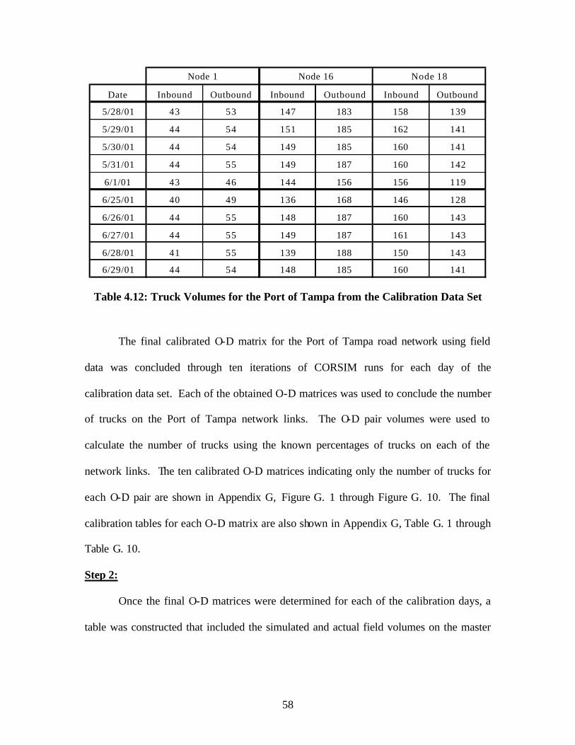
58
Date Inbound Outbound Inbound Outbound Inbound Outbound
5/28/01 43 53 147 183 158 139
5/29/01 44 54 151 185 162 141
5/30/01 44 54 149 185 160 141
5/31/01 44 55 149 187 160 142
6/1/01 43 46 144 156 156 119
6/25/01 40 49 136 168 146 128
6/26/01 44 55 148 187 160 143
6/27/01 44 55 149 187 161 143
6/28/01 41 55 139 188 150 143
6/29/01 44 54 148 185 160 141
Node 1 Node 16 Node 18
Table 4.12: Truck Volumes for the Port of Tampa from the Calibration Data Set
The final calibrated O-D matrix for the Port of Tampa road network using field
data was concluded through ten iterations of CORSIM runs for each day of the
calibration data set. Each of the obtained O-D matrices was used to conclude the number
of trucks on the Port of Tampa network links. The O-D pair volumes were used to
calculate the number of trucks using the known percentages of trucks on each of the
network links. The ten calibrated O-D matrices indicating only the number of trucks for
each O-D pair are shown in Appendix G, Figure G. 1 through Figure G. 10. The final
calibration tables for each O-D matrix are also shown in Appendix G, Table G. 1 through
Table G. 10.
Step 2:
Once the final O-D matrices were determined for each of the calibration days, a
table was constructed that included the simulated and actual field volumes on the master

59
links for each day (5/28/2001 to 6/1/2001 and 6/25/2001 to 6/29/2001). The data is
summarized in Table 4.13.
Date Field Simulated Field Simulated Field Simulated Field Simulated Field Simulated Field Simulated Field Simulated Field Simulated
28-May 170 167 165 169 124 129 141 135 110 105 91 88 158 155 117 124
29-May 154 157 169 179 120 124 115 116 91 94 85 89 159 156 118 113
30-May 160 167 163 170 129 123 143 136 93 95 85 88 154 155 115 110
31-May 169 167 161 169 132 134 134 136 95 94 87 90 150 155 119 114
1-Jun 177 169 161 169 134 128 145 138 99 96 91 88 142 148 120 115
25-Jun 179 172 126 129 93 95 87 88 156 155 112 114
26-Jun 174 167 134 128 93 97 83 86 158 156 113 108
27-Jun 159 166 132 126 94 95 89 88 153 155 114 109
28-Jun 167 169 134 128 98 95 90 88 159 154 114 116
29-Jun 167 168 134 128 99 96 80 84 120 115
22nd St 21st St.SR-92 (N) SR-92 (S) 50th Street (N) 50th Street (S) Causeway Blvd. (E) Causeway Blvd. (W)
Note: empty cells in the table indicate equipment failure or data was not available.
Table 4.13: Field and Simulated Truck Volumes on the Master Links (Calibration Data Set)
Step 3:
The simulated and actual volumes on these master links for all the calibration
days were compared. The comparisons include visual inspection and a Confidence
Interval statistical test. The Confidence Interval (C.I.) is a reliable approach for
comparing a simulation model with the real-world system (15). The C.I. was performed
for m collected independent sets of data from the system and n independent sets of data
from the model (m and n can be equal). Let Xj be the average of observations in the jth set
of system data with mean µx = E (Xj) and let Yj be the output from the jth replication of
the simulation model with µy = E (Yj).
The objective is to build a confidence- interval for:
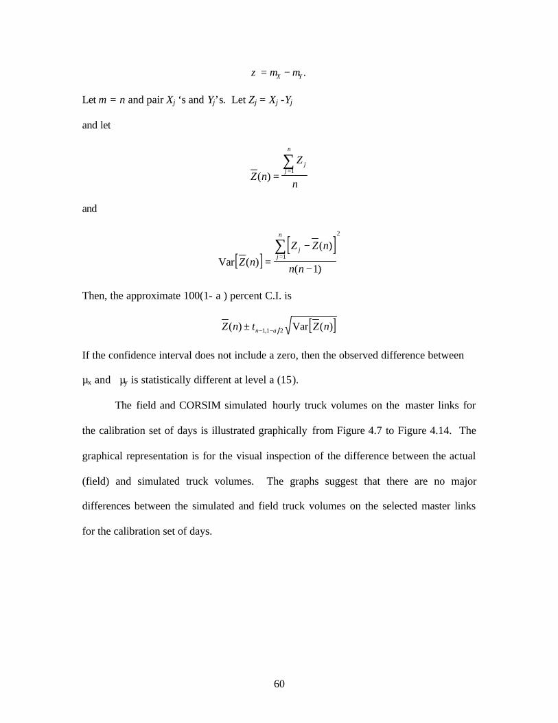
60
ζ µ µ= −X Y .
Let m = n and pair Xj ‘s and Yj’s. Let Zj = Xj -Yj
and let
Z nZ
n
jj
n
( ) ==
∑1
and
[ ][ ]
Var Z nZ Z n
n n
jj
n
( )( )
( )=
−
−=
∑1
2
1
Then, the approximate 100(1- a ) percent C.I. is
[ ]Z n t Z nn( ) ( ),± − −1 1 2α Var
If the confidence interval does not include a zero, then the observed difference between
µx and µy is statistically different at level a (15).
The field and CORSIM simulated hourly truck volumes on the master links for
the calibration set of days is illustrated graphically from Figure 4.7 to Figure 4.14. The
graphical representation is for the visual inspection of the difference between the actual
(field) and simulated truck volumes. The graphs suggest that there are no major
differences between the simulated and field truck volumes on the selected master links
for the calibration set of days.

61
140
145
150
155
160
165
170
175
180
185
1 2 3 4 5 6 7 8 9 10
Day Number
Tru
ck V
olum
e
Field Simulated
Figure 4.7: Field vs. CORSIM Simulated Truck Volumes on SR 92 Northbound
(Calibration)
150
155
160
165
170
175
180
185
1 2 3 4 5
Day Number
Tru
ck V
olum
e
Field Simulated
Figure 4.8: Field vs. CORSIM Simulated Truck Volumes on SR 92 Southbound
(Calibration)

62
110
115
120
125
130
135
140
1 2 3 4 5 6 7 8 9 10
Day Number
Tru
ck V
olum
e
Field Simulated
Figure 4.9: Field vs. CORSIM Simulated Truck Volumes on 50th Street Northbound
(Calibration)
0
20
40
60
80
100
120
140
160
1 2 3 4 5
Day Number
Tru
ck V
olum
e
Field
Simulated
Figure 4.10: Field vs. CORSIM Simulated Truck Volumes on 50th Street
Southbound (Calibration)

63
0
20
40
60
80
100
120
1 2 3 4 5 6 7 8 9 10
Day Number
Tru
ck V
olum
e
Field Simulated
Figure 4.11: Field vs. CORSIM Simulated Truck Volumes on Causeway Boulevard
Eastbound (Calibration)
74
76
78
80
82
84
86
88
90
92
1 2 3 4 5 6 7 8 9 10
Day Number
Tru
ck V
olum
e
Field Simulated
Figure 4.12: Field vs. CORSIM Simulated Truck Volumes on Causeway Boulevard
Westbound (Calibration)

64
130
135
140
145
150
155
160
165
1 2 3 4 5 6 7 8 9
Day Number
Tru
ck V
olum
e
Field Simulated
Figure 4.13: Field vs. CORSIM Simulated Truck Volumes on 22nd Street
(Calibration)
100
105
110
115
120
125
130
1 2 3 4 5 6 7 8 9 10
Day Number
Tru
ck V
olum
e
Field Simulated
Figure 4.14: Field vs. CORSIM Simulated Truck Volumes on 21st Street
(Calibration)

65
After the visual inspection showed no major differences between the simulated
and the actual truck volumes on the master links, a statistical test was performed for each
of the master links using the Confidence Interval (C.I.) Statistical Test. In Appendix H,
Figure H. 1 through Figure H. 4 shows the C.I. calculations for each master link. Table
4.14 summarizes the C.I. calculations. Upper and lower limits of the confidence interval
for each of the master links include zero. Therefore, the C.I. test concludes there is no
significant difference between the simulated and actual truck volumes on the master
links.
Link NameLower Limit
of CIUpper Limit
of CI
SR 92 N -5.1 7.1
SR 92 S -8.3 11.6
50th St N -11.8 25.1
50 th St. S -8.3 11.6
Causeway E -2.7 2.0
Causeway W -2.2 4.2
22nd St -2.7 2.7
21st St -12.3 26.8
Table 4.14: Confidence Interval Limits for the Truck Volumes on the Master Links (Calibration)
It can be concluded after conducting these two tests (visual inspection and
Confidence Interval test) that each of the ten CORSIM calibrated truck O-D matrices
replicate the existing conditions of the truck movements for the Port of Tampa at the 95%
confidence level.

66
As mentioned earlier, the O-D matrix that represents the existing conditions for
the Port of Tampa road network is the average of the 10 final calibrated O-D matrices.
This O-D matrix is shown in Figure 4.15. Nodes 1, 16, and 18 are indicated with “Port”
because they are external nodes directly associated with the Port of Tampa. Table 4.15
shows the simulated truck volumes that were calculated from the CORSIM output after
loading the network with the final calibrated O-D matrix. Table 4.15 also shows the
average of the calibration data set (23 days) of field truck volumes and the absolute
percent error between the simulated and field truck volumes for the master links. Two
thirds of the field data (23 days) were used for testing the accuracy of the final O-D
matrix.
The absolute percent error for every master link is less than 5% (formula shown
below). These results conclude that the final O-D matrix (Figure 4.15) represents the real
world (existing conditions) for the Port of Tampa road network. Figure 4.16 is a
graphical representation of average field and simulated truck volumes for the master
links.
100% ∗−
=Field
SimulatedFieldError
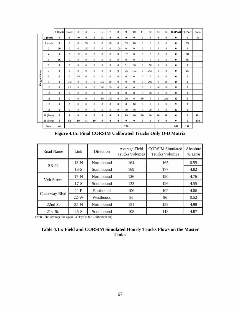
67
1 (Port) 1 south 3 4 5 6 7 8 9 10 11 12 13 14 16 (Port) 18 (Port) Sum.
1 (Port) 0 0 40 0 0 13 0 0 0 0 0 0 0 0 0 0 53
1 south 0 0 0 50 0 0 20 0 53 10 0 0 0 0 0 39
3 20 0 0 100 0 0 0 100 0 0 0 0 0 0 0 0
4 0 0 100 0 0 0 0 0 32 0 0 0 0 0 0 58
5 16 0 0 0 0 0 0 0 0 0 0 0 0 0 0 36
6 8 0 0 0 0 0 0 0 51 60 0 78 0 0 0 0
7 0 0 0 0 0 0 0 0 26 152 0 260 0 0 0 25
8 0 0 76 0 0 0 0 0 0 0 0 0 0 0 0 0
9 0 143 0 4 0 150 10 0 0 0 0 200 0 10 24 0
10 0 15 0 0 0 100 30 0 0 0 0 0 40 30 16 0
11 0 0 0 0 0 0 0 0 0 0 0 60 0 0 38 0
12 0 0 0 0 0 80 120 0 20 0 60 0 0 216 10 0
13 0 0 0 0 0 0 0 0 0 10 0 0 0 0 23 0
14 0 0 0 0 0 0 0 0 30 40 0 79 0 0 36 0
16 (Port) 0 0 0 0 0 0 0 5 19 40 80 10 10 18 0 0 181
18 (Port) 0 62 10 41 10 0 8 8 0 0 0 0 0 0 0 0 138
Sum. 44 230 147 157
Ori
gin
Nod
es
Figure 4.15: Final CORSIM Calibrated Trucks Only O-D Matrix
Road Name Link DirectionAverage Field
Trucks VolumesCORSIM Simulated
Trucks VolumesAbsolute % Error
13-N Northbound 164 165 0.55
13-S Southbound 169 177 4.82
17-N Northbound 126 120 4.76
17-S Southbound 132 126 4.55
22-E Eastbound 106 102 4.06
22-W Westbound 86 86 0.52
22nd St 25-N Northbound 151 158 4.98
21st St. 25-S Southbound 108 113 4.87
SR-92
50th Street
Causeway Blvd
(Note: The Average for Up to 23 Days in the Calibration set)
Table 4.15: Field and CORSIM Simulated Hourly Trucks Flows on the Master Links

68
0
20
40
60
80
100
120
140
160
180
200
SR-92-N SR-92-S 50th Street- N
50th Street- S
CausewayBlvd E
CausewayBlvd W
22nd Street 21st Street
Road Name
Tru
ck V
olum
e
Field Volumes
Simulated Volumes
Figure 4.16:Field Vs CORSIM Simulated Truck Volumes for the Master Links
(Final Calibrated O-D Matrix)
4.2.2 Port of Tampa Network Model Calibration: VISSIM
For comparison of the two simulation packages, the same calibration procedure
used in CORSIM was applied to VISSIM. Calibration of the O-D matrix used in the
VISSIM model was performed using the same FDOT data, field data, and selected master
links. Also, the same initial O-D matrix for CORSIM was used. The same constraints
for the O-D matrix and conditions for the shortest path used in the CORSIM calibration
were applied to the VISSIM calibration procedure. However, VISSIM calculates the
shortest path between the external nodes of the network and assigns the traffic to different
routes based on Kirchoff's law.
69
∑=
−
−
= n
kk
jj
tt
ttroutep
1
)(α
α
where j = 1 ...n
• Where P denotes the probability of using a specific route, • n denotes the number of routes for a given origin-destination relation and • tt j is the travel time on route “j”.
An exponent value (∝) of 3.5 was used in this research.
Figure D. 2, shows selected output values from a VISSIM output data sample.
The VISSIM output file has the extension VLZ. It contains the travel time section
number, the average delay per vehicle at that section, number of vehicles, the average
delay per person, and the number of people in these vehicles. Each section represents a
predefined data collection point on the road network.
Calibration Using FDOT Data
To obtain the O-D matrix with minimum error using the FDOT data, 17 iterations
were performed. The last five consequent iterations are explained in following
paragraphs. The input of each consecutive simulation run is an adjusted O-D matrix and
the output is the simulated flows for all the links in the network. The initial O-D matrix
is the same used for the initial calibration with CORSIM, see Appendix I Figure I. 1. The
absolute percent error between the simulated and FDOT traffic volumes is calculated for
each link. The absolute percent error for a selected link equals the difference between the
FDOT and simulated volumes divided by the FDOT volume (formula shown below).
100% ∗−
=FDOT
SimulatedFDOTError

70
Thirteenth Iteration:
Table I. 1 in Appendix I shows the results from the 13th interation. On Link 24
(inbound) the error is high at 47.39%. This is similar to the error produced in a CORSIM
run (Table F. 1). It was concluded from the VISSIM output that Links 24 and 30 are part
of the shortest path between Node 7 and Node 10. The traffic volume of the 7-10 O-D
pair was increased to obtain higher traffic volumes on Links 24 and 30. The traffic
volume going from Node 7 to Node 10 was increased from 150 to 300 vehicles per hour
for the 14th iteration, see Appendix I Figure I. 2.
Fourteenth Iteration:
The 14th calibration table (Appendix I Table I. 2) shows that the percent errors for
Links 24 and 30 were significantly reduced. These improvements indicate that the
iterations are converging to a final acceptable O-D matrix. The new highest percent error
in Table I. 2 is for the traffic volume on Link 24 (outbound direction) at 31.31%. This
percent error has improved from the previous iteration by 16%. Another increase of 150
vph for the traffic volume of the 7-10 O-D pair was done for Link 24 increasing it from
300 to 450 vph. Figure I. 3 shows the O-D matrix for the 15th iteration.
Fifteenth Iteration:
Table I. 3 in Appendix I is the calibration table resulting from the 15th iteration.
The table shows significant improvement (reduction) in the percent error of the traffic
volumes on Link 24. The highest percent error is for the traffic volume on Link 14
(outbound direction) at 26.58%. It was concluded from the VISSIM output that Link 14
was part of the shortest path between Node 16 and Node 14. The traffic volume of the
16-14 O-D pair was decreased to obtain a lower traffic volume on Link 14. The traffic

71
volume from Node 16 to Node 14 was reduced from 350 to 200 vph in the next iteration
(see Figure I. 4). In order to compensate for the reduction at this port node (Node 16),
the O-D pair volumes between Node 16 and Nodes 8, 9, 10, 11, & 12 were increased by
150 vph. The 150 vph increase was distributed between the five nodes (8, 9, 10, 11, &
12) based on the traffic volume percentage each O-D pair contributes to the total volume
leaving the port at Node 16.
Sixteenth Iteration:
Table I. 4 in Appendix I is the calibration table resulting from the 16th iteration. The
percent error for the traffic volume on Link 14 (outbound direction) improved from
26.58% to 12.63%. The highest percent error was on Link 25 (outbound direction) at
15.93%. The VISSIM output showed that Link 25 was part of the shortest path between
Node 10 and Node 16. The traffic volume from Node 10 to Node 16 was reduced from
300 to 150 vph for the 17th iteration (see Figure I. 5). In order to compensate for the
reduction at this port node (Node 16), the O-D pair volumes between Nodes 8, 9, 11, 13,
& 14 and Node 16 were increased by a total of 150 vph. The 150 vph increase was
distributed between the five nodes (8, 9, 11, 13, & 14) based on the traffic volume
percentage each O-D pair contributes to the total volume leaving the port at Node 16.
Seventeenth Iteration (Final Iteration):
Table I. 5 in Appendix I is the calibration table resulting from the 17th iteration.
The percent error for the traffic on Link 25 (outbound direction) improved from 15.93%
to 6.91%. In this iteration, the absolute percent errors for all simulated volumes on the
selected master links were less than or equal to 15%. The calibrated O-D matrix of the
17th iteration is the initial O-D matrix for the field data calibration process. The VISSIM
72
FDOT data calibrated O-D matrix is the same as the CORSIM FDOT data calibrated O-D
matrix. VISSIM and CORSIM FDOT data calibrated O-D matrices are identical because
both packages use a travel time based algorithm for selecting the shortest path between
nodes.
Calibration Using Field Data
The next step is to calibrate (final calibration) the O-D matrix using field data
collected for the selected master links (#’s 13, 17, 22, and 25). The same 3-step process
used in CORSIM was performed using VISSIM to calibrate the O-D matrices in order to
achieve a final O-D matrix for the Port of Tampa road network.
Step 1:
The O-D volumes were modified using the same process explained previously.
The simulated volumes on the master links were required to match the field volumes for
the same links within an acceptable range of error. The same constraints for the O-D
matrices used in the CORSIM calibration were applied in the VISSIM calibration
procedure.
The field data calibrated O-D matrix for the Port of Tampa road network was
obtained through 7 iterations of VISSIM runs for each day of the calibration data set
(5/28/2001 to 6/01/2001 and 6/25/2001 to 6/29/2001). Each of the obtained O-D
matrices was used to conclude the number of trucks on the Port of Tampa network links.
The O-D pair volumes were used to calculate the number of trucks using the known
percentages of trucks on each network link. The final O-D matrices (obtained from the
VISSIM calibration) that produced minimum error (5% or less) between the simulated

73
and field truck volumes on the master links are the same as the matrices obtained using
CORSIM (Appendix G, Figure G. 1 through Figure G. 10). The final calibration tables
for each O-D matrix using VISSIM are shown in Appendix J, Table J. 1 through Table J.
10. The number of iterations to reach the final calibrated O-D matrix using VISSIM (7
iterations) was less than the number required using CORSIM (10 iterations). This
difference in the number of iterations between VISSIM and CORSIM is due to the way
an O-D matrix is entered in VISSIM. VISSIM’s tabular form is more simplified than that
for CORSIM (graphical form). Therefore, using CORSIM consumes more time and
effort than VISSIM to track the O-D pairs that need to be modified in the calibration
process.
Step 2:
Once the final O-D matrices were determined for each of the calibration days, a
table was constructed that included the simulated and actual field volumes on the master
links for each day selected for calibration (5/28/2001 to 6/1/2001 and 6/25/2001 to
6/29/2001). The data is summarized in Table 4.16.
Date Field Simulated Field Simulated Field Simulated Field Simulated Field Simulated Field Simulated Field Simulated Field Simulated
28-May 170 168 165 168 124 126 141 137 110 107 91 89 158 160 117 119
29-May 154 156 169 164 120 123 115 117 91 93 85 87 159 155 118 116
30-May 160 165 163 168 129 131 143 138 93 94 85 86 154 155 115 112
31-May 169 166 161 159 132 130 134 136 95 96 87 89 150 154 119 115
01-Jun 177 172 161 166 134 130 145 139 99 97 91 89 142 147 120 117
25-Jun 179 174 126 129 93 95 87 89 156 153 112 113
26-Jun 174 169 134 131 93 95 83 87 158 157 113 111
27-Jun 159 163 132 128 94 96 89 88 153 155 114 117
28-Jun 167 170 134 136 98 97 90 87 159 155 114 118
29-Jun 167 168 134 130 99 97 80 83 120 117
SR-92 (N) SR-92 (S) 50th Street (N) 50th Street (S) Causeway Blvd. (E)Causeway Blvd. (W) 22nd St 21st St.
Table 4.16: Field and VISSIM Simulated Truck Volumes on the Master Links (Calibration)
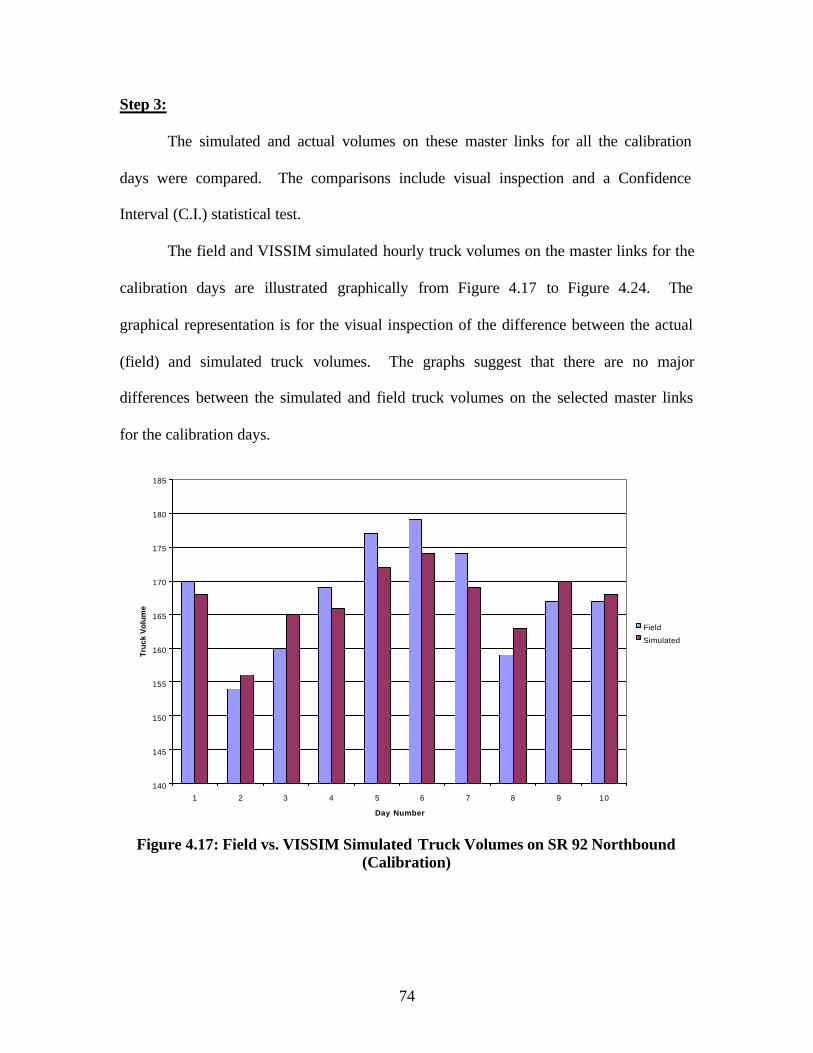
74
Step 3:
The simulated and actual volumes on these master links for all the calibration
days were compared. The comparisons include visual inspection and a Confidence
Interval (C.I.) statistical test.
The field and VISSIM simulated hourly truck volumes on the master links for the
calibration days are illustrated graphically from Figure 4.17 to Figure 4.24. The
graphical representation is for the visual inspection of the difference between the actual
(field) and simulated truck volumes. The graphs suggest that there are no major
differences between the simulated and field truck volumes on the selected master links
for the calibration days.
140
145
150
155
160
165
170
175
180
185
1 2 3 4 5 6 7 8 9 10
Day Number
Truc
k V
olum
e
Field
Simulated
Figure 4.17: Field vs. VISSIM Simulated Truck Volumes on SR 92 Northbound
(Calibration)

75
154
156
158
160
162
164
166
168
170
1 2 3 4 5
Day Number
Tru
ck V
olu
me
Field
Simulated
Figure 4.18: Field vs. VISSIM Simulated Truck Volumes on SR 92 Southbound
(Calibration)
110
115
120
125
130
135
140
1 2 3 4 5 6 7 8 9 1 0
Day Number
Truc
k V
olum
e
Field
Simulated
Figure 4.19: Field vs. VISSIM Simulated Truck Volumes on 50th Street Northbound
(Calibration)

76
0
20
40
60
80
100
120
140
160
1 2 3 4 5
Day Number
Tru
ck V
olu
me
Field
Simulated
Figure 4.20: Field vs. VISSIM Simulated Truck Volumes on 50th Street Southbound
(Calibration)
0
2 0
4 0
6 0
8 0
1 0 0
1 2 0
1 2 3 4 5 6 7 8 9 10
Day Number
Truc
k V
olum
e
Field
Simulated
Figure 4.21: Field vs. VISSIM Simulated Truck Volumes on Causeway Boulevard
Eastbound (Calibration)

77
74
76
78
80
82
84
86
88
90
92
1 2 3 4 5 6 7 8 9 10
Day Number
Tru
ck V
olu
me
Field
Simulated
Figure 4.22: Field vs. VISSIM Simulated Truck Volumes on Causeway Boulevard
Westbound (Calibration)
130
135
140
145
150
155
160
165
1 2 3 4 5 6 7 8 9
Day Number
Truc
k V
olum
e
Field
Simulated
Figure 4.23: Field vs. VISSIM Simulated Truck Volumes on 22nd Street
(Calibration)

78
106
108
110
112
114
116
118
120
122
1 2 3 4 5 6 7 8 9 10
Day Number
Truc
k V
olum
e
Field
Simulated
Figure 4.24: Field vs. VISSIM Simulated Truck Volumes on 21st Street (Calibration)
After the visual inspection showed no major differences between the simulated
and the actual truck volumes on the master links, a statistical test was performed for each
of the master links using the Confidence Interval (C.I.) Statistical Test. In Appendix K,
Figure K. 1 through Figure K. 4 shows the C.I. calculations for each master link. Table
4.17 summarizes the C.I. calculations. Upper and lower limits of the confidence interval
for each of the master links include zero. Therefore, the C.I. test concludes there is no
significant difference between the simulated and actual truck volumes on the master
links.

79
Link NameLower Limit
of CIUpper Limit
of CI
SR 92 N -3.6 3.4
SR 92 S -3.4 13.4
50th St N -3.1 2.2
50 th St. S -6.6 6.9
Causeway E -1.4 1.1
Causeway W -1.7 2.5
22nd St -2.3 2.5
21st St -3.3 2.2
Table 4.17: Confidence Interval Limits for the Difference between Actual and VISSIM Simulated Truck Volumes (Calibration)
It can be concluded after conducting these two tests (visual inspection and
Confidence Interval test) tha t each of the ten VISSIM calibrated truck O-D matrices
replicate the existing conditions of the truck movements for the Port of Tampa at the 95%
confidence level.
As mentioned earlier, the O-D matrix that represents the existing conditions for
the Port of Tampa road network is the average of the 10 final calibrated O-D matrices.
This O-D matrix is shown in Figure 4.15. Nodes 1, 16, and 18 are indicated with “Port”
because they are external nodes directly associated with the Port of Tampa. Table 4.18
shows the simulated truck volumes that were calculated from the VISSIM output after
loading the network with the final calibrated O-D matrix. Table 4.18 also shows the
average of the calibration data set (23 days) of field truck volumes and the absolute
percent error between the simulated and field truck volumes for the master links.

80
The absolute percent error for every master link is less than 5% (formula shown
below). These results conclude that the final O-D matrix (Figure 4.15) represents the real
world (existing conditions) for the Port of Tampa road network. Figure 4.25 is a
graphical representation of average field and simulated truck volumes for the master
links.
100% ∗−
=Field
SimulatedFieldError
Road Name Link DirectionAverage Field
Trucks VolumesVISSIM Simulated Trucks Volumes
Absolute % Error
13-N Northbound 164 167 1.77
13-S Southbound 169 174 2.96
17-N Northbound 126 123 2.38
17-S Southbound 132 128 3.03
22-E Eastbound 106 103 2.83
22-W Westbound 86 88 2.56
22nd St 25-N Northbound 151 155 2.82
21st St. 25-S Southbound 108 105 2.51
SR-92
50th Street
Causeway Blvd
Note: The Average for Up to 23 Days in the Calibration set
Table 4.18: Field and VISSIM Simulated Truck Volumes of the Master Links

81
0
20
40
60
80
100
120
140
160
180
200
SR-92-N SR-92-S 50th Street- N
50th Street- S
CausewayBlvd E
CausewayBlvd W
22nd Street 21st Street
Road Name
Tru
ck V
olum
e
Field VolumesSimulated Volumes
Figure 4.25: Field and VISSIM Simulated Volumes for the Master Links
4.3 Route Assignment Model Validation
The purpose of the validation step is to check the applicability of the
developed models to any day other than the set of days used in the calibration process.
The 11 weekdays selected for validation (7/5/2001 to 7/10/2001 and 7/16/ 2001 to
7/23/2001) is from the data in Table 4.6. The validation data set should be
comprehensive for all data collection locations. The validation process was performed
for both CORSIM and VISSIM models independently. The general steps to perform the
validation are as follows:

82
Step 1:
Feed the model with the number of trucks leaving or entering on the Port of Tampa's
access roads for each of the days in the validation data set. All other O-D pair volumes
are the same as those in the final calibrated O-D matrix (Figure 4.15). The port' s access
roads are represented in the O-D matrix by Node 1 (Port Sutton and Pendola Point
Roads), Node 16 (22nd and 20th Street), and Node 18 (Causeway Boulevard). The
number of trucks leaving and entering the port for any day was obtained by entering the
vessel freight data for that day into the truck trip generation model for the Port of Tampa
(11). The output of this model is the number of trucks leaving or entering the Port of
Tampa for each of the access roads (Nodes 1, 16, and 18). The daily number of trucks
leaving/entering the Port of Tampa in July 2001 (validation period) is shown in Appendix
F, Table F. 1 & Table F. 2.
The truck trip generation model produces only daily truck volumes. However, the
simulation models require peak hourly volumes. Therefore, conversion factors from
daily truck volumes to the total traffic volumes and then to the peak hourly volumes were
used. The first factor that converts the truck volume to the relevant total traffic volume is
the truck factor (T). The truck factors are known for the traffic volume at each of the
three entrances and exits (Nodes 1, 16, and 18) from the field counts that were conducted
at these locations during Phase II of the project. The second factor (K factor) is the ratio
between the peak hourly volume and the daily volume. The K factors are also known for
each of the three entrances and exits (Nodes 1, 16, and 18) from the field counts
conducted at these locations during Phase II. Table 4.19 summarizes the T and K factors
for the entrance and exit nodes at the Port of Tampa.

83
Node Truck Factor K Factor Truck Factor K Factor
1 0.4 0.08 0.4 0.08
16 0.2 0.09 0.12 0.1
18 0.23 0.09 0.22 0.09
Inbound Outbound
Table 4.19: T & K Factors for the Port of Tampa
For each day in the validation data set (from 7/5/2001 to 7/10/2001 and from
7/16/ 2001 to 7/24/2001), the peak hourly truck volume was calculated using Error!
Reference source not found.. Multiplying the daily number of trucks by the K factor
determines the peak hour truck volume. The truck volumes used in the validation process
are shown in Table 4.20.
Date Inbound Outbound Inbound Outbound Inbound Outbound
7/5/01 44 40 152 198 110 136
7/6/01 43 40 144 198 105 136
7/9/01 41 39 139 196 101 135
7/10/01 40 39 135 195 98 134
7/16/01 42 40 143 197 104 135
7/17/01 40 39 136 196 99 134
7/18/01 39 39 133 196 97 134
7/19/01 40 39 135 195 98 134
7/20/01 42 40 143 197 104 135
7/23/01 41 34 139 170 101 117
7/24/01 45 34 153 171 112 117
7/25/01 47 40 158 200 115 137
Node 1 Node 16 Node 18
Table 4.20: Total Number of Trucks Entering and Leaving the Port of Tampa on
Validation Set of Days
Step 2
Run the simulation model and obtain the simulated volumes on the master links.
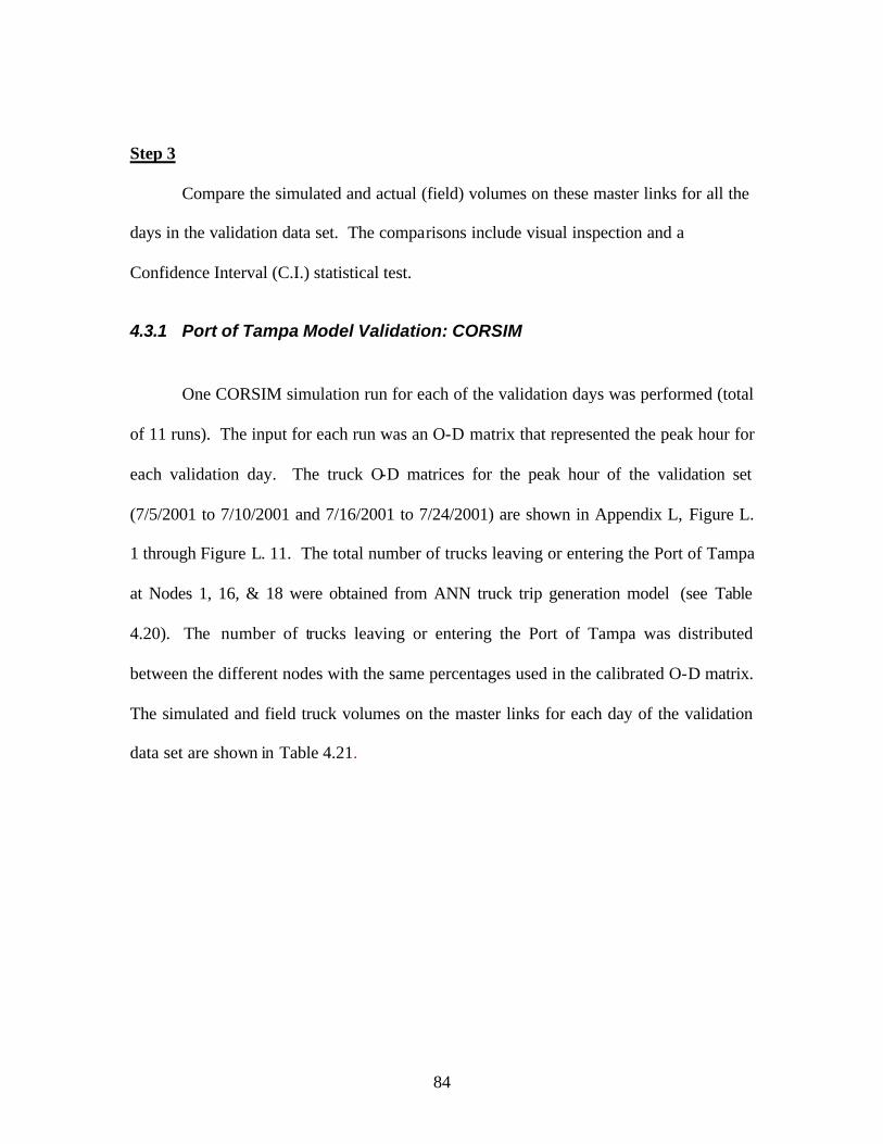
84
Step 3
Compare the simulated and actual (field) volumes on these master links for all the
days in the validation data set. The comparisons include visual inspection and a
Confidence Interval (C.I.) statistical test.
4.3.1 Port of Tampa Model Validation: CORSIM
One CORSIM simulation run for each of the validation days was performed (total
of 11 runs). The input for each run was an O-D matrix that represented the peak hour for
each validation day. The truck O-D matrices for the peak hour of the validation set
(7/5/2001 to 7/10/2001 and 7/16/2001 to 7/24/2001) are shown in Appendix L, Figure L.
1 through Figure L. 11. The total number of trucks leaving or entering the Port of Tampa
at Nodes 1, 16, & 18 were obtained from ANN truck trip generation model (see Table
4.20). The number of trucks leaving or entering the Port of Tampa was distributed
between the different nodes with the same percentages used in the calibrated O-D matrix.
The simulated and field truck volumes on the master links for each day of the validation
data set are shown in Table 4.21.

85
Dates Field Simulated Field Simulated Field Simulated Field Simulated Field Simulated Field Simulated Field Simulated Field Simulated
07/05/2001 208 218 242 237 168 160 161 160 140 133 130 124 184 178 127 126
07/06/2001 234 224 211 221 168 161 154 156 127 121 124 118 196 190 137 132
07/09/2001 222 220 233 236 153 155 153 160 130 124 120 116 184 178 142 137
07/10/2001 223 219 253 239 154 156 191 184 124 118 124 119 182 178 123 127
07/16/2001 217 220 227 233 147 153 175 167 124 120 136 131 164 170 120 126
07/17/2001 230 224 220 230 182 174 173 165 148 141 124 118 197 189 126 122
07/18/2001 219 220 231 234 186 179 170 162 119 121 118 115 192 184 150 143
07/19/2001 216 220 228 236 188 181 171 163 101 104 108 114 186 181 133 127
07/20/2001 214 220 241 234 174 156 161 157 122 123 91 95 184 190 157 131
07/23/2001 242 230 230 236 150 155 167 160 121 116 125 119 178 184 136 132
07/24/2001 230 222 221 228 155 157 161 160 124 119 123 125 198 189 121 125
50th Street (S)50th Street (N)SR-92 (S)SR-92 (N) 21st St22nd stCauseway (W)Causeway (E)
Table 4.21: Field and Simulated Truck Volumes of the Master Links
The field and CORSIM simulated truck volumes for the master links are
illustrated graphically from Figure 4.26 to Figure 4.33. The graphical representation is
for the visual inspection to observe the difference between the actual (field) and
simulated truck volumes. The graphs suggest that there are no major differences between
the simulated and the field truck volumes of the master links on the validation set of days
(11 weekdays).

86
190
200
210
220
230
240
250
1 2 3 4 5 6 7 8 9 10 11
Day Number
Tru
ck V
olum
e
Field
CORSIM
Figure 4.26: Field vs. CORSIM Simulated Truck Volumes on SR 92 Northbound
(Validation)
180
190
200
210
220
230
240
250
260
1 2 3 4 5 6 7 8 9 10 11
Day Number
Tru
ck V
olum
e
Field
CORSIM
Figure 4.27: Field vs. CORSIM Simulated Truck Volumes on SR 92 Southbound
(Validation)

87
0
20
40
60
80
100
120
140
160
180
200
1 2 3 4 5 6 7 8 9 10 11
Day Number
Tru
ck V
olum
e
Field
CORSIM
Figure 4.28: Field vs. CORSIM Simulated Truck Volumes on 50th Street
Northbound (Validation)
0
50
100
150
200
250
1 2 3 4 5 6 7 8 9 10 11
Day Number
Tru
ck V
olum
e
Field
CORSIM
Figure 4.29: Field vs. CORSIM Simulated Truck Volumes on 50th Street
Southbound (Validation)

88
0
20
40
60
80
100
120
140
160
1 2 3 4 5 6 7 8 9 10 11
Day Number
Tru
ck V
olum
es
Field
CORSIM
Figure 4.30: Field vs. CORSIM Simulated Truck Volumes on Causeway Blvd
Eastbound (Validation)
0
20
40
60
80
100
120
140
160
1 2 3 4 5 6 7 8 9 10 11
Day Number
Tru
ck V
olum
e
Field
CORSIM
Figure 4.31: Field vs. CORSIM Simulated Truck Volumes on Causeway Blvd
Westbound (Validation)
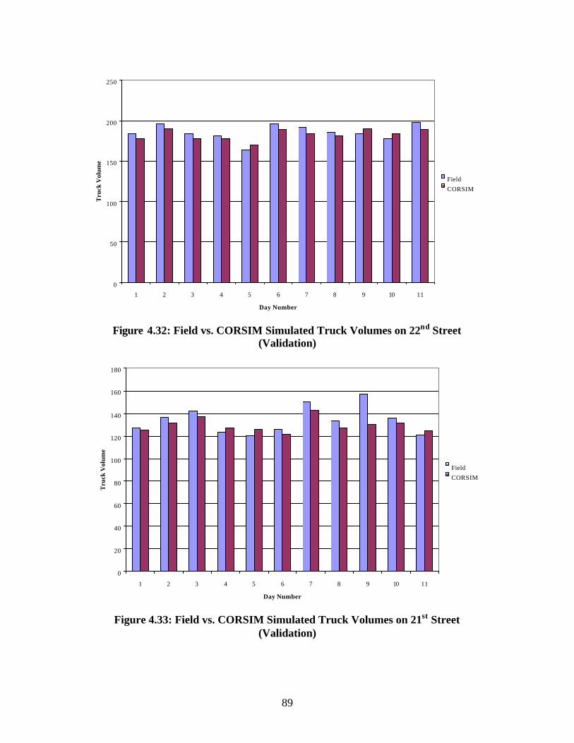
89
0
50
100
150
200
250
1 2 3 4 5 6 7 8 9 10 11
Day Number
Tru
ck V
olum
e
Field
CORSIM
Figure 4.32: Field vs. CORSIM Simulated Truck Volumes on 22nd Street
(Validation)
0
20
40
60
80
100
120
140
160
180
1 2 3 4 5 6 7 8 9 10 11
Day Number
Tru
ck V
olum
e
FieldCORSIM
Figure 4.33: Field vs. CORSIM Simulated Truck Volumes on 21st Street
(Validation)

90
After the visual inspection showed no major differences between the simulated
and the actual truck volumes on the master links, a statistical test was performed for each
of the master links using the Confidence Interval (C.I.) Statistical Test. In Appendix M,
Figure M. 1 to Figure M. 4 shows the C.I. calculations for each master link. Table 4.22
summarizes the C.I. calculations. Upper and lower limits of the confidence interval for
each of the master links include zero. Therefore, the C.I. test concludes there is no
significant difference between the simulated and actual truck volumes on the master
links.
Link NameLower Limit
of CIUpper Limit
of CI
SR 92 N -9.2 5.6
SR 92 S -8.7 16.8
50th St N -26.8 12.7
50 th St. S -16.0 7.6
Causeway E -25.8 12.6
Causeway W -26.3 12.7
22nd St -18.9 10.7
21st St -23.1 11.5
Table 4.22: Confidence Interval Limits for the Difference between Actual and CORSIM Simulated Truck Volumes
It can be concluded after conducting these two tests (visual inspection and
Confidence Interval test) that each of the ten CORSIM calibrated truck O-D matrices
replicate the existing conditions of the truck movements for the Port of Tampa at the 95%
confidence level.

91
4.3.2 Port of Tampa Model Validation: VISSIM
The same validation steps for CORSIM were conducted using VISSIM. One
VISSIM simulation run for each of the validation days was performed (total of 11 runs).
The input for each run was an O-D matrix that represented the peak hour for each
validation day. The truck O-D matrices for the peak hour of the validation set (7/5/2001
to 7/10/2001 and 7/16/2001 to 7/24/2001) are shown in Appendix L, Figure L. 1 to
Figure L. 11. The total numbers of trucks leaving or entering the Port of Tampa at Nodes
1, 16, & 18 were obtained from the truck trip generation model (Table 4.20). The
number of trucks leaving or entering the Port of Tampa were distributed between the
different nodes with the same percentages used in the calibrated O-D matrix. The
VISSIM simulated and field truck volumes on the master links for each day of the
validation data set are shown in Table 4.23.

92
SR-92 (N) SR-92 (S) 50th Street (N) 50th Street (S)Date Field VISSIM Field VISSIM Field VISSIM Field VISSIM
7/5/2001 208 212 242 243 168 162 161 1657/6/2001 234 229 211 215 168 171 154 1557/9/2001 222 217 233 239 153 149 153 1487/10/2001 223 220 253 246 154 153 191 1807/16/2001 217 226 227 235 147 146 175 1687/17/2001 230 234 220 211 182 186 173 1637/18/2001 219 217 231 237 186 187 170 1777/19/2001 216 214 228 231 188 192 171 1647/20/2001 214 212 241 240 174 170 161 1587/23/2001 242 244 230 234 150 153 167 1647/24/2001 230 238 221 216 155 154 161 157
Causeway Blvd (E) Causeway Blvd (W) 22nd Street 21st StreetDate Field VISSIM Field VISSIM Field VISSIM Field VISSIM
7/5/2001 140 134 130 124 184 179 127 1307/6/2001 127 126 124 123 196 192 137 1357/9/2001 130 125 120 120 184 176 142 1377/10/2001 124 118 124 123 182 179 123 1257/16/2001 124 121 136 137 164 167 120 1257/17/2001 148 148 124 126 197 185 126 1267/18/2001 119 114 118 125 192 184 150 1547/19/2001 101 105 108 113 186 178 133 1287/20/2001 122 118 91 93 184 178 157 1567/23/2001 121 118 125 126 178 181 136 1297/24/2001 124 119 123 122 198 189 121 123
Table 4.23: Field and VISSIM Simulated Truck Volumes of the Master Links
The field and VISSIM simulated truck volumes for the master links are illustrated
graphically from Figure 4.34 to Figure 4.41. The graphical representation is for the
visual inspection to observe the difference between the actual (field) and simulated truck
volumes. The graphs suggest that there are no major differences between the simulated
and the field truck volumes of the master links on the validation set of days (11
weekdays).

93
190
200
210
220
230
240
250
1 2 3 4 5 6 7 8 9 10 11
Day Number
Tru
ck V
olum
e
FieldVISSIM
Figure 4.34: Field vs. VISSIM Simulated Truck Volumes on SR 92 Northbound
(Validation)
180
190
200
210
220
230
240
250
260
1 2 3 4 5 6 7 8 9 10 11
Day Number
Tru
ck V
olum
e
Field
VISSIM
Figure 4.35: Field vs. VISSIM Simulated Truck Volumes on SR 92 Southbound
(Validation)
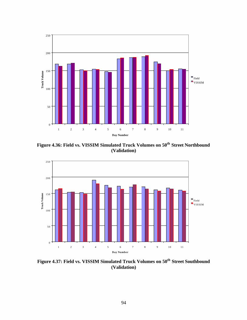
94
0
50
100
150
200
250
1 2 3 4 5 6 7 8 9 10 11
Day Number
Tru
ck V
olum
e
FieldVISSIM
Figure 4.36: Field vs. VISSIM Simulated Truck Volumes on 50th Street Northbound
(Validation)
0
50
100
150
200
250
1 2 3 4 5 6 7 8 9 10 11
Day Number
Tru
ck V
olum
e
Field
VISSIM
Figure 4.37: Field vs. VISSIM Simulated Truck Volumes on 50th Street Southbound
(Validation)
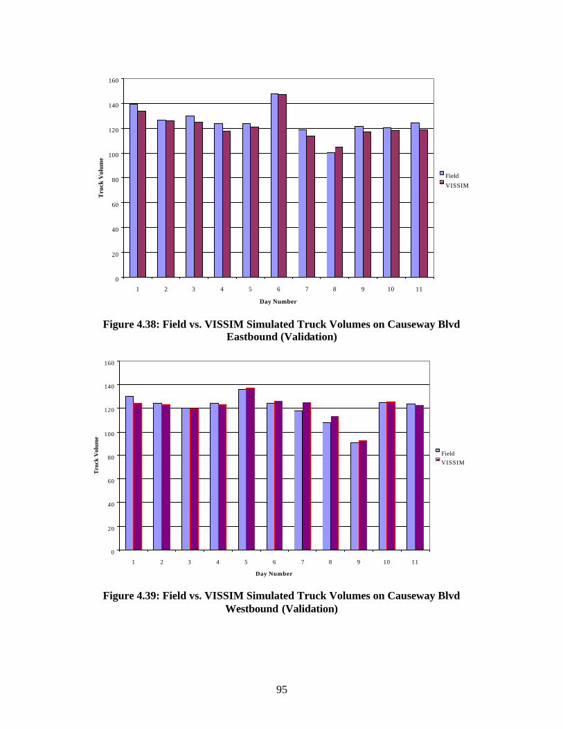
95
0
20
40
60
80
100
120
140
160
1 2 3 4 5 6 7 8 9 10 11
Day Number
Tru
ck V
olum
e
Field
VISSIM
Figure 4.38: Field vs. VISSIM Simulated Truck Volumes on Causeway Blvd
Eastbound (Validation)
0
20
40
60
80
100
120
140
160
1 2 3 4 5 6 7 8 9 10 11
Day Number
Tru
ck V
olum
e
FieldVISSIM
Figure 4.39: Field vs. VISSIM Simulated Truck Volumes on Causeway Blvd
Westbound (Validation)

96
0
50
100
150
200
250
1 2 3 4 5 6 7 8 9 10 11
Day Number
Tru
ck V
olum
e
FieldVISSIM
Figure 4.40: Field vs. VISSIM Simulated Truck Volumes on 22nd Street (Validation)
0
20
40
60
80
100
120
140
160
180
1 2 3 4 5 6 7 8 9 10 11
Day Number
Tru
ck V
olum
e
Field
VISSIM
Figure 4.41: Field vs. VISSIM Simulated Truck Volumes on 21st Street (Validation)
After the visual inspection showed no major differences between the simulated
and the actual truck volumes on the master links, a statistical test was performed for each
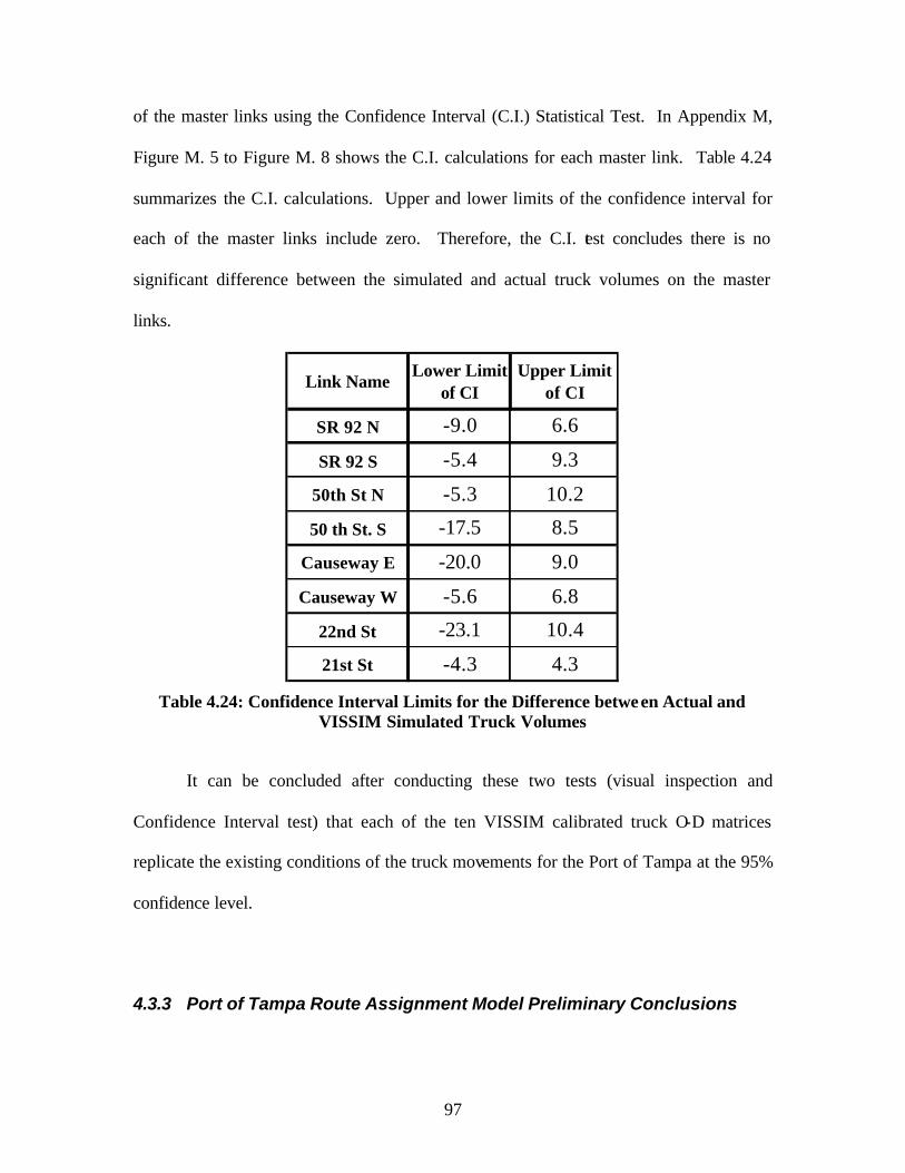
97
of the master links using the Confidence Interval (C.I.) Statistical Test. In Appendix M,
Figure M. 5 to Figure M. 8 shows the C.I. calculations for each master link. Table 4.24
summarizes the C.I. calculations. Upper and lower limits of the confidence interval for
each of the master links include zero. Therefore, the C.I. test concludes there is no
significant difference between the simulated and actual truck volumes on the master
links.
Link NameLower Limit
of CIUpper Limit
of CI
SR 92 N -9.0 6.6
SR 92 S -5.4 9.3
50th St N -5.3 10.2
50 th St. S -17.5 8.5
Causeway E -20.0 9.0
Causeway W -5.6 6.8
22nd St -23.1 10.4
21st St -4.3 4.3
Table 4.24: Confidence Interval Limits for the Difference between Actual and VISSIM Simulated Truck Volumes
It can be concluded after conducting these two tests (visual inspection and
Confidence Interval test) that each of the ten VISSIM calibrated truck O-D matrices
replicate the existing conditions of the truck movements for the Port of Tampa at the 95%
confidence level.
4.3.3 Port of Tampa Route Assignment Model Preliminary Conclusions

98
The O-D matrix that represents the existing conditions for the Port of Tampa road
network is shown in Figure 4.42.
1 (Port) 1 south 3 4 5 6 7 8 9 10 11 12 13 14 16 (Port) 18 (Port) Sum.
1 (Port) 0 0 40 0 0 13 0 0 0 0 0 0 0 0 0 0 53
1 south 0 0 0 50 0 0 20 0 53 10 0 0 0 0 0 39
3 20 0 0 100 0 0 0 100 0 0 0 0 0 0 0 0
4 0 0 100 0 0 0 0 0 32 0 0 0 0 0 0 58
5 16 0 0 0 0 0 0 0 0 0 0 0 0 0 0 36
6 8 0 0 0 0 0 0 0 51 60 0 78 0 0 0 0
7 0 0 0 0 0 0 0 0 26 152 0 260 0 0 0 25
8 0 0 76 0 0 0 0 0 0 0 0 0 0 0 0 0
9 0 143 0 4 0 150 10 0 0 0 0 200 0 10 24 0
10 0 15 0 0 0 100 30 0 0 0 0 0 40 30 16 0
11 0 0 0 0 0 0 0 0 0 0 0 60 0 0 38 0
12 0 0 0 0 0 80 120 0 20 0 60 0 0 216 10 0
13 0 0 0 0 0 0 0 0 0 10 0 0 0 0 23 0
14 0 0 0 0 0 0 0 0 30 40 0 79 0 0 36 0
16 (Port) 0 0 0 0 0 0 0 5 19 40 80 10 10 18 0 0 181
18 (Port) 0 62 10 41 10 0 8 8 0 0 0 0 0 0 0 0 138
Sum. 44 230 147 157
Ori
gin
Nod
es
Figure 4.42: Existing Conditions O-D matrix for the Port of Tampa
It was observed from the final O-D matrix that the total number of trucks leaving
the Port of Tampa at Node 16 (22nd St and 20th St) during the peak hour is 181 trucks.
The number of trucks leaving the Port of Tampa from Node 16 and traveling towards
Node 11 (I-4 & I-275 interchange) is 80 trucks (44% of total number of trucks leaving at
Node 16). Link 10 (I-4) is part of the shortest path between Node 16 and Node 11. This
means that 44% of trucks (80 trucks) leaving the port at Node 16 are using I-4 towards I-
275. The final O-D matrix also shows that 22% of the trucks (40 trucks) leaving the port
at Node 16 are traveling towards Node 10 (I-4 & 22nd St. interchange). The number of
trucks leaving the Port from Node 16 and traveling towards Node 9 (interchange between

99
I-4 and SR 41) is 19 trucks. It was concluded that 77% of the trucks leaving the port at
Node 16 (142 trucks) are using I-4 during the peak hour.
The number of trucks leaving the Port of Tampa at Node 18 (Causeway
Boulevard) during the peak hour is 138 trucks. The number of trucks that are leaving the
Port of Tampa from Node 18 and traveling towards Node 1 (SR 41 south) is 62 trucks
(45% of the total trucks leaving the port at Node 18). Also, the number of trucks leaving
the Port of Tampa at Causeway Boulevard and traveling towards Node 4 (I-75) is 41
trucks. This means that 29% of the trucks leaving the port from Node 18 are using
Causeway Boulevard to access I-75.
The number of trucks leaving the Port of Tampa at Node 1 (Pendola Point and
Port Sutton) in the peak hour is 53 trucks. The number of trucks leaving the port at Node
1 and traveling towards Node 3 (SR 301) is 40 trucks (75% of the total trucks leaving at
this node). Only 13 trucks originating from the port at Node 1 will exit the network at
Node 6 (SR 618).
The number of trucks entering the Port of Tampa at Node 16 (22nd St. and 20th
St.) during the peak hour is 147 trucks. The number of trucks entering the Port and
originating from Node 9 (SR 41 and I-4 interchange) is 24 trucks (16% of the total trucks
entering the port at Node 16). The number of trucks entering the port and originating
from Node 11 (I-275/I-4 interchange) is 38 trucks (25% of the total trucks entering the
port at Node 16). Since Links 9 and 10 are both I-4 links and are part of the shortest path
between Nodes 9-16 and 11-16, it was determined that 43% of the trucks (62 trucks)
entering the port at Node 16 are using I-4.

100
The number of trucks entering the Port of Tampa at Node 18 (Causeway
Boulevard) during the peak hour is 157 trucks. The number of trucks entering the port at
Node 18 and originating from Node 1 (SR 41 south) is 39 trucks (25% of the total trucks
entering the port at Node 18). Also, the number of trucks entering the Port of Tampa on
Causeway Boulevard and originating from Node 4 (I-75) is 58 trucks (38%). The
number of trucks entering the port at Node 18 that are coming from Node 5 (intersection
between SR 301 and Causeway Boulevard) is 36 trucks (23% of the total trucks entering
the port at the Causeway Boulevard entrance).
The number of trucks entering the Port of Tampa at Node 1 (Pendola Point and
Port Sutton) in the peak hour is 44 trucks. The number of trucks entering the port at
Node 1 and originating from node 3 (SR 301) is 20 trucks (45% of the total trucks
entering the port at this node). The number of trucks entering the port at Node 1 and
originating from Node 5 (intersection between SR 301 and Causeway Boulevard) is 16
trucks (36% of the total trucks entering at this node). Table 4.25 summarizes these
conclusions.
Direction TotalNumber of
TrucksPercentage
Number of Trucks
PercentageNumber of
TrucksPercentage
Outbound 372 142 38% 80 22% 41 11%
Inbound 348 78 22% 38 11% 20 6%
I-4 I-275 I-75
Note: % refers to trucks entering/leaving at the indicated interstate node
Table 4.25: Peak Hour Truck Volumes on the Interstate Highways Generated by Port of Tampa Freight Activity

101
Table 4.25 shows the total number of trucks leaving the Port of Tampa during the
peak hour (372 trucks) and the number of trucks using each of the adjacent interstate
highways. It also shows the percentages of the total truck volumes entering or leaving
the Port of Tampa and using the different interstate highways.
The existing major routes for trucks generated by the Port of Tampa’s freight
activity are the highlighted routes shown in Figure 4.43. One of these routes is SR 676.
This route connects the Port of Tampa (Node 18) with SR 301 & I-75 and carries (40
trucks per hour) about 30% of the trucks leaving the port from Node 18. Another route is
on 22nd Street that connects the Port of Tampa (Node 16) with I-4 and consequently to I-
275. This route carries (154 trucks per hour) 78% of the trucks leaving the port from
Node 16.
SR 676
SR 41
I-4
22nd
St
N-18
N-1
N-16
Figure 4.43: Major Truck Routes on the Port of Tampa Road Network

102
From the comparison between the CORSIM and VISSIM simulation packages,
both can be used to solve a truck assignment problem through simulation. Both packages
produced similar results; however VISSIM is more user friendly than CORSIM. The
truck volumes from the field are compared to both the CORSIM and VISSIM simulated
output values for the selected master links during the peak hour for the validation data set
and are presented graphically in Figure 4.44 to Figure 4.51.
190
200
210
220
230
240
250
1 2 3 4 5 6 7 8 9 10 11
Day Number
Tru
ck V
olum
e
Field
CORSIM
VISSIM
Figure 4.44: Field, CORSIM Simulated and VISSIM Simulated Truck Volumes for SR 92 Northbound
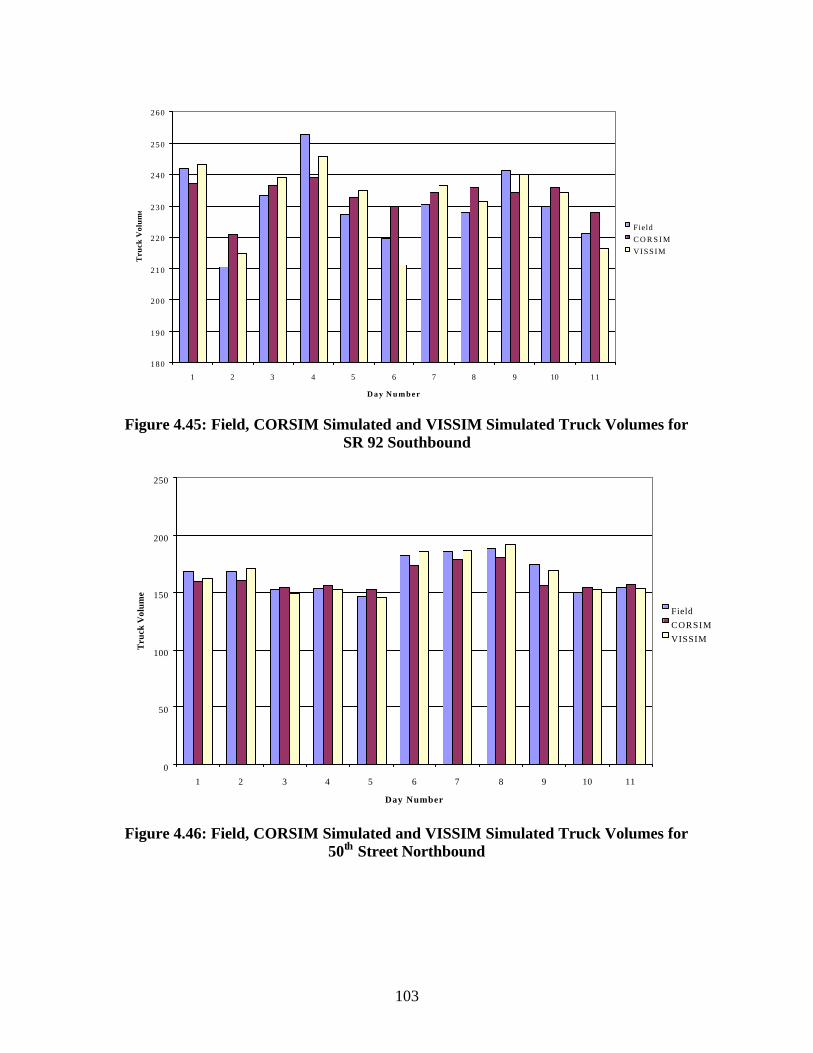
103
180
190
200
210
220
230
240
250
260
1 2 3 4 5 6 7 8 9 10 11
D a y N u m b e r
Tru
ck V
olum
e
FieldC O R S I M VISSIM
Figure 4.45: Field, CORSIM Simulated and VISSIM Simulated Truck Volumes for
SR 92 Southbound
0
50
100
150
200
250
1 2 3 4 5 6 7 8 9 10 11
Day Number
Tru
ck V
olum
e
Field
CORSIM
VISSIM
Figure 4.46: Field, CORSIM Simulated and VISSIM Simulated Truck Volumes for
50th Street Northbound

104
0
50
100
150
200
250
1 2 3 4 5 6 7 8 9 10 11
Day Number
Tru
ck V
olum
e
FieldCORSIM
VISSIM
Figure 4.47: Field, CORSIM Simulated and VISSIM Simulated Truck Volumes for
50th Street Southbound
0
20
40
60
80
100
120
140
160
1 2 3 4 5 6 7 8 9 10 11
Day Number
Tru
ck V
olum
e
Field
CORSIM VISSIM
Figure 4.48: Field, CORSIM Simulated and VISSIM Simulated Truck Volumes for
Causeway Boulevard Eastbound
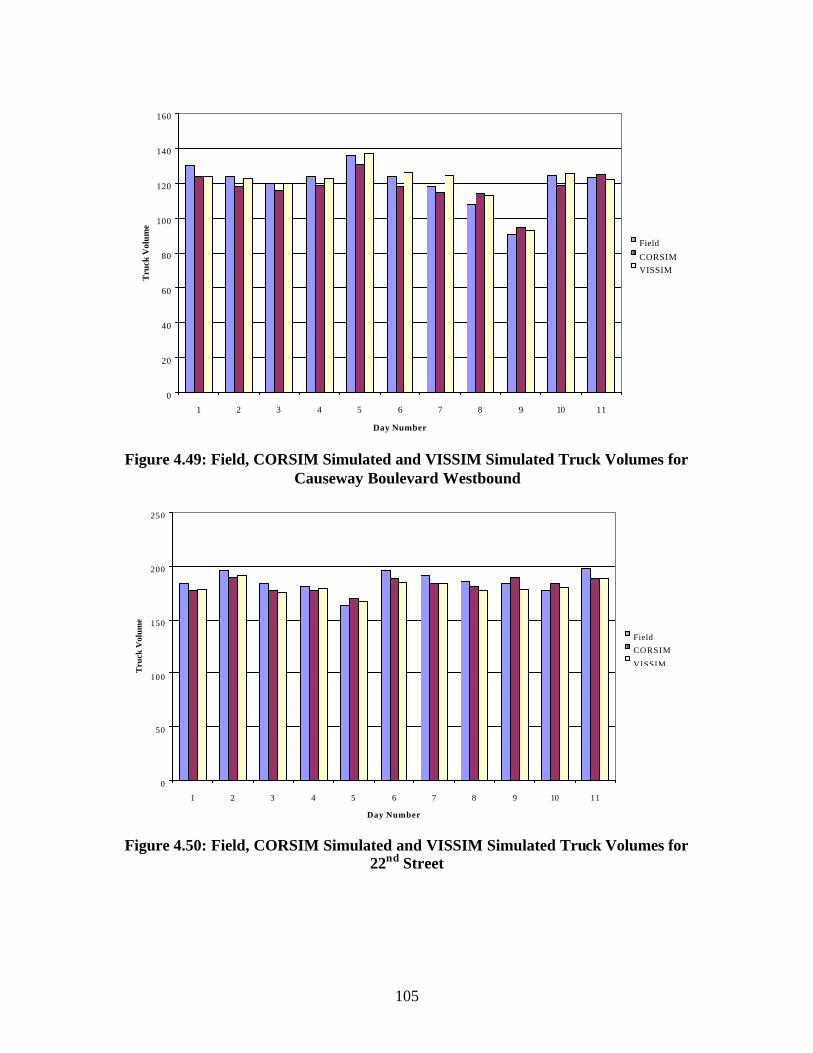
105
0
20
40
60
80
100
120
140
160
1 2 3 4 5 6 7 8 9 10 11
Day Number
Tru
ck V
olum
e
Field
CORSIM VISSIM
Figure 4.49: Field, CORSIM Simulated and VISSIM Simulated Truck Volumes for
Causeway Boulevard Westbound
0
50
100
150
200
250
1 2 3 4 5 6 7 8 9 10 11
Day Number
Tru
ck V
olum
e
FieldCORSIM
VISSIM
Figure 4.50: Field, CORSIM Simulated and VISSIM Simulated Truck Volumes for
22nd Street
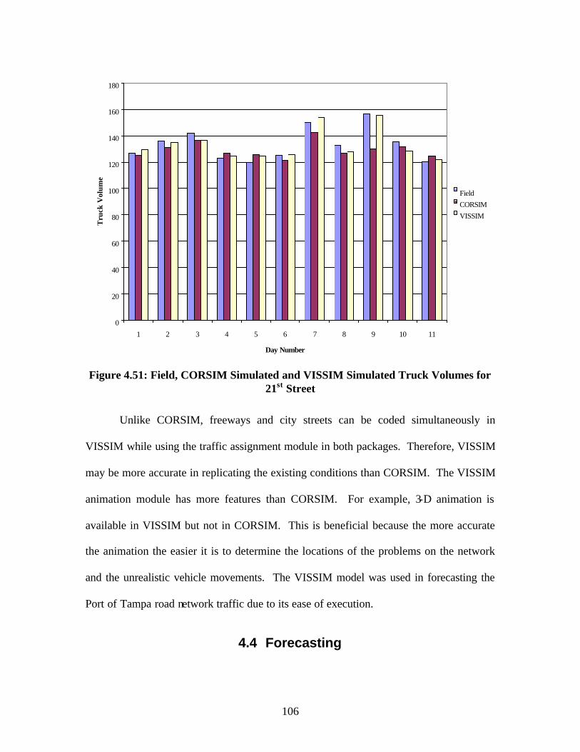
106
0
20
40
60
80
100
120
140
160
180
1 2 3 4 5 6 7 8 9 10 11
Day Number
Tru
ck V
olum
e
FieldCORSIM VISSIM
Figure 4.51: Field, CORSIM Simulated and VISSIM Simulated Truck Volumes for
21st Street
Unlike CORSIM, freeways and city streets can be coded simultaneously in
VISSIM while using the traffic assignment module in both packages. Therefore, VISSIM
may be more accurate in replicating the existing conditions than CORSIM. The VISSIM
animation module has more features than CORSIM. For example, 3-D animation is
available in VISSIM but not in CORSIM. This is beneficial because the more accurate
the animation the easier it is to determine the locations of the problems on the network
and the unrealistic vehicle movements. The VISSIM model was used in forecasting the
Port of Tampa road network traffic due to its ease of execution.
4.4 Forecasting
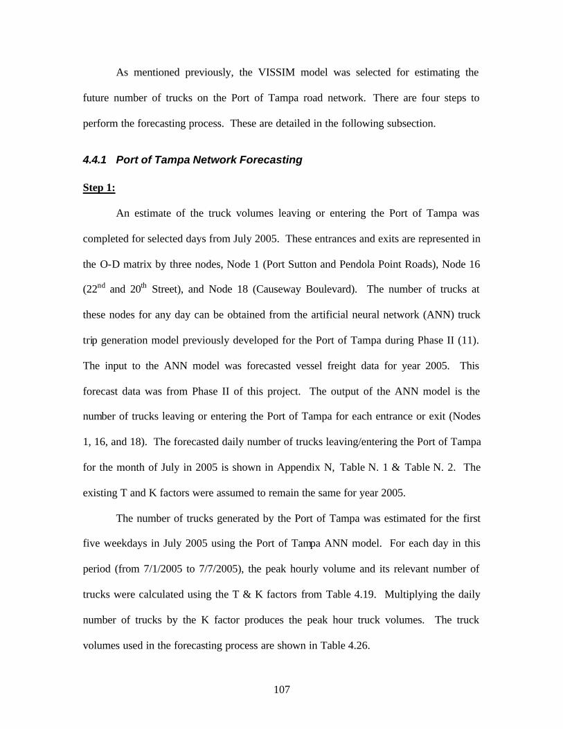
107
As mentioned previously, the VISSIM model was selected for estimating the
future number of trucks on the Port of Tampa road network. There are four steps to
perform the forecasting process. These are detailed in the following subsection.
4.4.1 Port of Tampa Network Forecasting Step 1:
An estimate of the truck volumes leaving or entering the Port of Tampa was
completed for selected days from July 2005. These entrances and exits are represented in
the O-D matrix by three nodes, Node 1 (Port Sutton and Pendola Point Roads), Node 16
(22nd and 20th Street), and Node 18 (Causeway Boulevard). The number of trucks at
these nodes for any day can be obtained from the artificial neural network (ANN) truck
trip generation model previously developed for the Port of Tampa during Phase II (11).
The input to the ANN model was forecasted vessel freight data for year 2005. This
forecast data was from Phase II of this project. The output of the ANN model is the
number of trucks leaving or entering the Port of Tampa for each entrance or exit (Nodes
1, 16, and 18). The forecasted daily number of trucks leaving/entering the Port of Tampa
for the month of July in 2005 is shown in Appendix N, Table N. 1 & Table N. 2. The
existing T and K factors were assumed to remain the same for year 2005.
The number of trucks generated by the Port of Tampa was estimated for the first
five weekdays in July 2005 using the Port of Tampa ANN model. For each day in this
period (from 7/1/2005 to 7/7/2005), the peak hourly volume and its relevant number of
trucks were calculated using the T & K factors from Table 4.19. Multiplying the daily
number of trucks by the K factor produces the peak hour truck volumes. The truck
volumes used in the forecasting process are shown in Table 4.26.
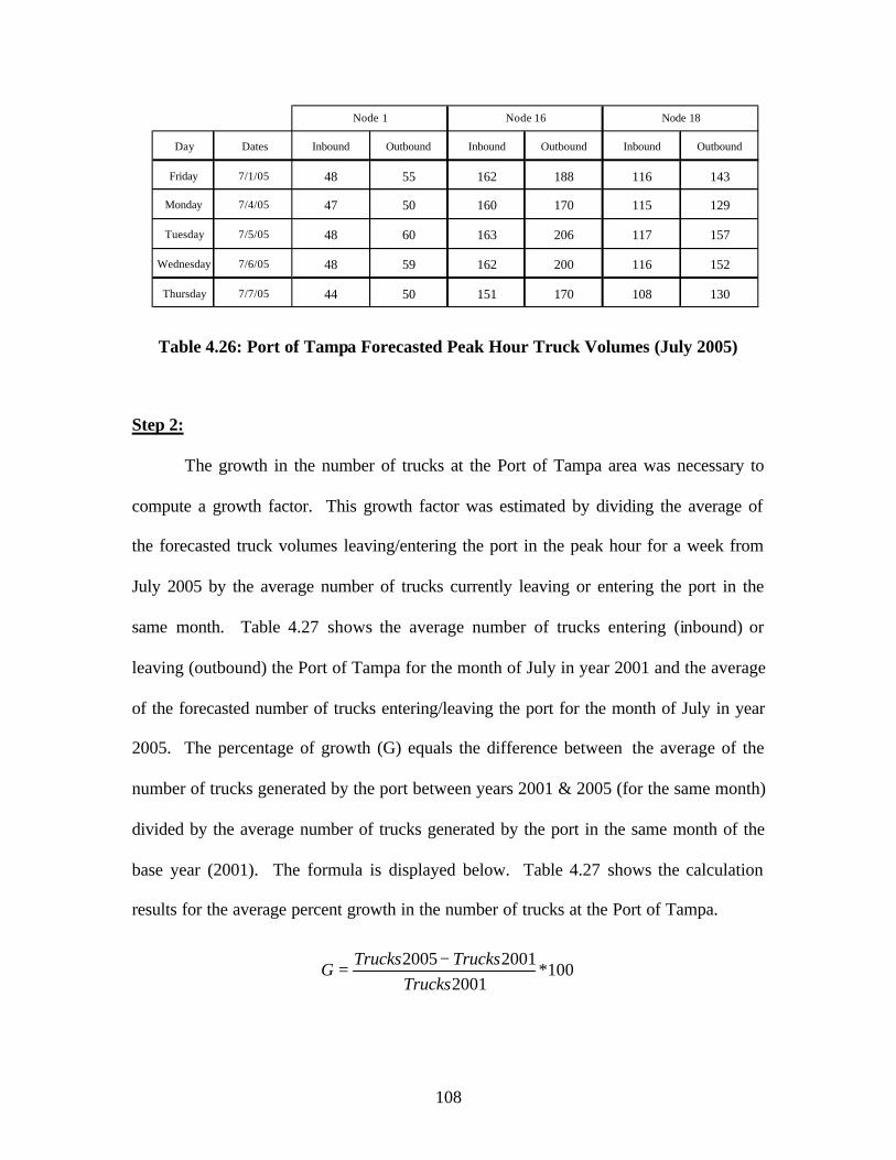
108
Day Dates Inbound Outbound Inbound Outbound Inbound Outbound
Friday 7/1/05 48 55 162 188 116 143
Monday 7/4/05 47 50 160 170 115 129
Tuesday 7/5/05 48 60 163 206 117 157
Wednesday 7/6/05 48 59 162 200 116 152
Thursday 7/7/05 44 50 151 170 108 130
Node 1 Node 16 Node 18
Table 4.26: Port of Tampa Forecasted Peak Hour Truck Volumes (July 2005)
Step 2:
The growth in the number of trucks at the Port of Tampa area was necessary to
compute a growth factor. This growth factor was estimated by dividing the average of
the forecasted truck volumes leaving/entering the port in the peak hour for a week from
July 2005 by the average number of trucks currently leaving or entering the port in the
same month. Table 4.27 shows the average number of trucks entering (inbound) or
leaving (outbound) the Port of Tampa for the month of July in year 2001 and the average
of the forecasted number of trucks entering/leaving the port for the month of July in year
2005. The percentage of growth (G) equals the difference between the average of the
number of trucks generated by the port between years 2001 & 2005 (for the same month)
divided by the average number of trucks generated by the port in the same month of the
base year (2001). The formula is displayed below. Table 4.27 shows the calculation
results for the average percent growth in the number of trucks at the Port of Tampa.
100*2001
20012005Trucks
TrucksTrucksG
−=

109
Inbound Outbound
July Year 2001 295 370
July Year 2005 321 384
Percentage of Growth 8% 4%
Average Number of Trucks
Average Percentage of Growth
6%
Table 4.27: Average Percentage of Growth in the Number of Trucks
Step 3:
The O-D matrix for the forecast days in July 2005 was determined by multiplying
all the volumes of the final O-D matrix for current conditions excluding the volumes for
the port nodes (#’s 1, 16, & 18) by 1.06 (1 + growth factor). The port nodes are changed
according to the estimated traffic volumes computer from the output of the ANN model.
Step 4:
The forecasted number of trucks leaving or entering the port at Nodes 1, 16, & 18
shown in Table 4.26 was distributed between the different nodes. The forecasted truck
volumes are distributed using the existing percent of trucks for each O-D pair from the
total. The O-D matrices for the first five weekdays of July 2005 (excluding the July 4th
holiday) are shown in Figure 4.52 to Figure 4.55.
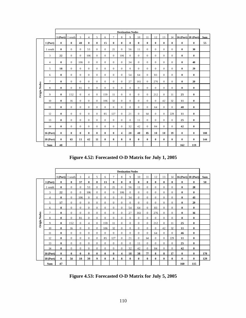
110
1 (Port) 1 south 3 4 5 6 7 8 9 10 11 12 13 14 16 (Port) 18 (Port) Sum
1 (Port) 0 0 40 0 0 15 0 0 0 0 0 0 0 0 0 0 55
1 south 0 0 0 53 0 0 21 0 56 11 0 0 0 0 0 30
3 22 0 0 106 0 0 0 106 0 0 0 0 0 0 0 0
4 0 0 106 0 0 0 0 0 34 0 0 0 0 0 0 40
5 18 0 0 0 0 0 0 0 0 0 0 0 0 0 0 29
6 8 0 0 0 0 0 0 0 54 64 0 83 0 0 0 0
7 0 0 0 0 0 0 0 0 27 161 0 276 0 0 0 20
8 0 0 81 0 0 0 0 0 0 0 0 0 0 0 0 0
9 0 152 0 4 0 159 11 0 0 0 0 212 0 11 25 0
10 0 16 0 0 0 106 32 0 0 0 0 0 42 32 11 0
11 0 0 0 0 0 0 0 0 0 0 0 64 0 0 48 0
12 0 0 0 0 0 85 127 0 21 0 64 0 0 229 11 0
13 0 0 0 0 0 0 0 0 0 11 0 0 0 0 25 0
14 0 0 0 0 0 0 0 0 32 42 0 84 0 0 42 0
16 (Port) 0 0 0 0 0 0 0 4 20 40 85 10 10 19 0 0 188
18 (Port) 0 63 11 42 11 0 8 8 0 0 0 0 0 0 0 0 144
Sum 48 162 119
Ori
gin
Nod
es
Destination Nodes
Figure 4.52: Forecasted O-D Matrix for July 1, 2005
1 (Port) 1 south 3 4 5 6 7 8 9 10 11 12 13 14 16 (Port) 18 (Port) Sum
1 (Port) 0 0 37 0 0 13 0 0 0 0 0 0 0 0 0 0 50
1 south 0 0 0 53 0 0 21 0 56 11 0 0 0 0 0 28
3 22 0 0 106 0 0 0 106 0 0 0 0 0 0 0 0
4 0 0 106 0 0 0 0 0 34 0 0 0 0 0 0 43
5 17 0 0 0 0 0 0 0 0 0 0 0 0 0 0 29
6 8 0 0 0 0 0 0 0 54 64 0 83 0 0 0 0
7 0 0 0 0 0 0 0 0 27 161 0 276 0 0 0 16
8 0 0 81 0 0 0 0 0 0 0 0 0 0 0 0 0
9 0 152 0 4 0 159 11 0 0 0 0 212 0 11 25 0
10 0 16 0 0 0 106 32 0 0 0 0 0 42 32 11 0
11 0 0 0 0 0 0 0 0 0 0 0 64 0 0 46 0
12 0 0 0 0 0 85 127 0 21 0 64 0 0 229 11 0
13 0 0 0 0 0 0 0 0 0 11 0 0 0 0 25 0
14 0 0 0 0 0 0 0 0 32 42 0 84 0 0 42 0
16 (Port) 0 0 0 0 0 0 0 4 18 38 77 8 8 17 0 0 170
18 (Port) 0 54 10 39 9 0 8 8 0 0 0 0 0 0 0 0 129
Sum 47 160 115
Destination Nodes
Ori
gin
Nod
es
Figure 4.53: Forecasted O-D Matrix for July 5, 2005

111
1 (Port) 1 south 3 4 5 6 7 8 9 10 11 12 13 14 16 (Port) 18 (Port) Sum
1 (Port) 0 0 43 0 0 17 0 0 0 0 0 0 0 0 0 0 60
1 south 0 0 0 53 0 0 21 0 56 11 0 0 0 0 0 28
3 22 0 0 106 0 0 0 106 0 0 0 0 0 0 0 0
4 0 0 106 0 0 0 0 0 34 0 0 0 0 0 0 45
5 18 0 0 0 0 0 0 0 0 0 0 0 0 0 0 29
6 8 0 0 0 0 0 0 0 54 64 0 83 0 0 0 0
7 0 0 0 0 0 0 0 0 27 161 0 276 0 0 0 16
8 0 0 81 0 0 0 0 0 0 0 0 0 0 0 0 0
9 0 152 0 4 0 159 11 0 0 0 0 212 0 11 25 0
10 0 16 0 0 0 106 32 0 0 0 0 0 42 32 11 0
11 0 0 0 0 0 0 0 0 0 0 0 64 0 0 49 0
12 0 0 0 0 0 85 127 0 21 0 64 0 0 229 11 0
13 0 0 0 0 0 0 0 0 0 11 0 0 0 0 25 0
14 0 0 0 0 0 0 0 0 32 42 0 84 0 0 42 0
16 (Port) 0 0 0 0 0 0 0 4 23 46 91 10 10 22 0 0 206
18 (Port) 0 66 12 45 14 0 10 10 0 0 0 0 0 0 0 0 157
Sum 48 163 117
Destination NodesO
rigi
n N
odes
Figure 4.54: Forecasted O-D Matrix for July 6, 2005
1 (Port) 1 south 3 4 5 6 7 8 9 10 11 12 13 14 16 (Port) 18 (Port) Sum
1 (Port) 0 0 43 0 0 16 0 0 0 0 0 0 0 0 0 0 59
1 south 0 0 0 53 0 0 21 0 56 11 0 0 0 0 0 28
3 22 0 0 106 0 0 0 106 0 0 0 0 0 0 0 0
4 0 0 106 0 0 0 0 0 34 0 0 0 0 0 0 44
5 18 0 0 0 0 0 0 0 0 0 0 0 0 0 0 29
6 8 0 0 0 0 0 0 0 54 64 0 83 0 0 0 0
7 0 0 0 0 0 0 0 0 27 161 0 276 0 0 0 16
8 0 0 81 0 0 0 0 0 0 0 0 0 0 0 0 0
9 0 152 0 4 0 159 11 0 0 0 0 212 0 11 25 0
10 0 16 0 0 0 106 32 0 0 0 0 0 42 32 11 0
11 0 0 0 0 0 0 0 0 0 0 0 64 0 0 48 0
12 0 0 0 0 0 85 127 0 21 0 64 0 0 229 11 0
13 0 0 0 0 0 0 0 0 0 11 0 0 0 0 25 0
14 0 0 0 0 0 0 0 0 32 42 0 84 0 0 42 0
16 (Port) 0 0 0 0 0 0 0 4 22 43 90 10 10 21 0 0 200
18 (Port) 0 64 12 44 13 0 10 10 0 0 0 0 0 0 0 0 153
Sum 48 162 116
Destination Nodes
Ori
gin
Nod
es
Figure 4.55: Forecasted O-D Matrix for July 7, 2005

112
4.4.2 Port of Tampa Network Forecasting Conclusions The O-D matrix of July 7th 2005 (Figure 4.55) shows the total number of trucks
leaving the Port of Tampa at Node 16 (22nd St. and 20th St.) during the peak hour is 200
trucks. The number of trucks leaving the port from Node 16 and traveling towards Node
11 (I-4/I-275 interchange) is 90 trucks (45% of the total truck volume leaving at Node
16). Link 10 (I-4) is part of the shortest path between Node 16 and Node 11. This
indicates that 45% of the trucks (90 trucks) leaving the port at Node 16 are using I-4 in
the direction of I-275. The final O-D matrix also shows that 22% of the trucks (43
trucks) leaving the port at Node 16 are traveling in the direction of Node 10 (I-4 & 22nd
St. ramps). The number of trucks exiting the port from Node 16 and traveling towards
Node 9 (interchange between I-4 and 22nd St.) is 22 trucks. Also, 77% of the trucks
leaving the port from Node 16 (155 trucks) are using the I-4 during the peak hour. The
number of trucks leaving the port from Node 16 and using I-4 is estimated to increase
from 142 (existing conditions) to 155 trucks in July 2005 (9% increase).
The number of trucks leaving the Port of Tampa at Node 18 (Causeway
Boulevard) during the peak hour is 153 trucks. The number of trucks leaving the Port of
Tampa from Node 18 and traveling towards Node 1 (SR 41 south) is 64 trucks (42% of
the total trucks leaving the port at Node 18). Also, the number of trucks leaving the Port
of Tampa at Causeway Boulevard and heading towards Node 4 (I-75) is 43 trucks. This
means that 28% of the trucks leaving the port from Node 18 are using Causeway
Boulevard to access I-75. The number of trucks leaving the port from Node 18 and using
I-75 will increase slightly from 41 trucks (existing conditions) to 43 trucks in July 2005.

113
The number of trucks leaving the Port of Tampa at Node 1 (Pendola Point and
Port Sutton) in the peak hour is 59 trucks. The number of trucks leaving the port at Node
1 and traveling towards Node 3 (SR 301) is 43 trucks (72% of the total trucks leaving at
Node 1). Only 16 trucks originating from the port at Node 1 will exit the network at
Node 6 (SR 618). The number of trucks leaving the port from Node 1 and using SR 301
will increase slightly from 41 trucks (existing conditions) to 43 trucks in July 2005.
The number of trucks entering the Port of Tampa at Node 16 (22nd St. and 20th
St.) during the peak hour is 162 trucks. The number of trucks entering the port and
originating from Node 9 (SR 41/I-4 interchange) is 25 trucks (16% of the total trucks
entering the port at Node 16). The number of trucks entering the port and originating
from Node 11 (I-275/I-4 interchange) is 48 trucks (29% of the total trucks entering the
Port at Node 16). Since Links 9 and 10 are both I-4 links and are part of the shortest path
between Nodes 9-16 and 11-16, it was determined that 45% of the trucks (73 trucks)
entering the port at Node 16 are using I-4. This shows an increase from 62 trucks
(existing conditions) to 73 trucks in July 2005 (17% increase).
The number of trucks entering the Port of Tampa at Node 18 (Causeway
Boulevard) during the peak hour is 116 trucks. The number of trucks entering the port at
Node 18 and originating from Node 1 (SR 41 south) is 28 trucks (27% of the total trucks
entering the port at Node 18). The number of trucks entering the port at Causeway
Boulevard and originating from Node 4 (I-75) is 44 trucks (38%). Therefore, 38% of the
trucks entering the port at Causeway Boulevard are using I-75. Also, the number of
trucks entering the port at Node 18 and coming from Node 5 (intersection between SR
301 and Causeway Boulevard) is 29 trucks (27% of the total trucks entering the port at

114
Causeway Boulevard). These numbers have decreased compared to the existing
conditions.
The number of trucks entering the Port of Tampa at Node 1 (Pendola Point and
Port Sutton) in the peak hour is 48 trucks. The number of trucks entering the port at
Node 1 and originating from Node 3 (SR 301) is 22 trucks (45% of the total trucks
entering the port at Node 1). The number of trucks entering the port at Node 1 and
originating from Node 5 (intersection between SR 301 and Causeway Boulevard) is 18
trucks (36% of the total trucks entering at Node 1). These truck volumes have increased
slightly when compared to the existing conditions. Table 4.28 summarizes these short
term forecasting results.
Direction TotalNumber of
TrucksPercentage
Number of Trucks
PercentageNumber of
TrucksPercentage
Outbound 423 155 37% 90 22% 43 11%
Inbound 329 73 22% 48 15% 44 14%
I-4 I-275 I-75
Table 4.28: Forecasted Peak Hour Truck Volumes on the Interstate Highways Generated by Port of Tampa Freight Activity
Table 4.28 shows the total number of trucks leaving the Port of Tampa during the
peak hour on July 5th 2005 (423 trucks) and the number of trucks using each of the
adjacent interstate highways. It also shows the percentage of trucks using these interstate
highways. 37% of the total number of trucks leaving the Port of Tampa are using I-4 and
22% of the total number of trucks leaving the port are using I-275. For inbound trucks,
22% of the total trucks coming to the Port of Tampa are using I-4, 15% are using I-275,
and 14% are using I-75.

115
4.5 Sensitivity Analysis
Introduction Four scenarios have been studied using VISSIM for a sensitivity analysis on the
Port of Tampa road network. For each scenario, average travel time and average delay
have been calculated for the entire network and for the major truck routes connected to
the port. Average travel time and average delay were chosen as measures of
effectiveness (MOEs) for each run because they are commonly used for measuring the
performance of a transportation system (14). Average travel time for a link/route on a
road network is the average time used for all vehicles to traverse this link from beginning
(origin) to the end (destination) during a specific period of time (usually peak hour).
Average delay for a link/route on a road network is the difference between the average
travel time during a specific period of time and the average travel time during the off-
peak period (free flow conditions). The major truck routes for the Port of Tampa road
network include SR 41 (Links 17 and 30), 21st & 22nd Streets (Link 25), I-4 (Links 9, 10,
and 11), and Causeway Boulevard (Links 22 and 20). Figure 4.56 shows the Port of
Tampa road network with the major truck routes identified with purple highlight lines.

116
2912
11
10
25
15
28
Node 16
Node 10Node 11
Node 12
Node 13
Figure 4.56: The Port of Tampa Road Network
For each scenario, average travel time and average delay were obtained from
VISSIM output for the entire network and for the major trucks routes. The highlighted
volumes in the existing condition O-D matrix shown in Figure 4.57 represent the O-D
pairs associated with the major routes. The average travel time and average delay for the
entire network was calculated by averaging the travel time or the average delay for all the
network links.
Causeway Boulevard (Links 20 & 22) is part of the shortest path associated with
the O-D pairs 18-3, 4-18, 18-4, 5-18, 18-5, and 7-18. 22nd and 21st Streets (Link 25) are
part of the shortest path associated with the O-D pairs 9-16, 16-9, 10-16, 16-10, 11-16,
and 16-11. Interstate 4 (Links 9 &10) is part of the shortest path associated with the O-D
pairs 9-16, 16-9, 11-16, and 16-11. SR 41 (Links 30 & 17) is part of the shortest path
associated with the O-D pairs 7-18, 9-16, and 16-19.

117
1 (Port) 1 south 3 4 5 6 7 8 9 10 11 12 13 14 16 (Port) 18 (Port)
1 (Port) 0 0 40 0 0 13 0 0 0 0 0 0 0 0 0 0
1 south 0 0 0 50 0 0 20 0 53 10 0 0 0 0 0 39
3 20 0 0 100 0 0 0 100 0 0 0 0 0 0 0 0
4 0 0 100 0 0 0 0 0 32 0 0 0 0 0 0 58
5 16 0 0 0 0 0 0 0 0 0 0 0 0 0 0 36
6 8 0 0 0 0 0 0 0 51 60 0 78 0 0 0 0
7 0 0 0 0 0 0 0 0 26 152 0 260 0 0 0 25
8 0 0 76 0 0 0 0 0 0 0 0 0 0 0 0 0
9 0 143 0 4 0 150 10 0 0 0 0 200 0 10 24 0
10 0 15 0 0 0 100 30 0 0 0 0 0 40 30 16 0
11 0 0 0 0 0 0 0 0 0 0 0 60 0 0 38 0
12 0 0 0 0 0 80 120 0 20 0 60 0 0 216 10 0
13 0 0 0 0 0 0 0 0 0 10 0 0 0 0 23 0
14 0 0 0 0 0 0 0 0 30 40 0 79 0 0 36 0
16 (Port) 0 0 0 0 0 0 0 5 19 40 80 10 10 18 0 0
18 (Port) 0 62 10 41 10 0 8 8 0 0 0 0 0 0 0 0
Destination Nodes
Ori
gin
Nod
es
Figure 4.57: Port of Tampa Road Network O-D Matrix for Existing Conditions
4.5.1 Scenario 1 (Base Scenario)
The first scenario evaluated the existing conditions of the network using the
measures of effectiveness (average travel time and average delay). This scenario was
used as a base for the comparisons between different scenarios. The Port of Tampa road
network was used in this run without any changes to the geometry or the traffic operation
parameters. The average travel time for the entire network is 329 seconds/vehicle. See
Appendix O, Table O. 1 for average travel times and average delays for each link. The
average travel times between the major O-D pairs are shown in Figure 4.58. The O-D
pairs associated with port Node 16 are highlighted. The average delay for the entire

118
network is 113 seconds/vehicle. The average delay for the same O-D pairs is shown in
Figure 4.59. See Figure 4.56 for the major truck routes for this scenario.
Nodes 3 4 5 9 10 11 16 18
4 462
5 346
7 568
9 354
10 115
11 350
16 342 167 361
18 548 441 353
Figure 4.58: Average Travel Time (sec/veh) Between Major O-D Pairs (Base Scenario)
Nodes 3 4 5 9 10 11 16 18
4 145
5 117
7 229
9 45
10 39
11 58
16 40 30 53
18 232 132 113 Figure 4.59: Average Delay (sec/veh) on the Major Truck Routes (Base Scenario)

119
4.5.2 Scenario 2
The second scenario adds one lane for the north and south directions of Link 25
(22nd Street and 21st Street). No changes to the geometry or the traffic operation
parameters except for the addition of one lane for both directions of Link 25 were made
to the network. The same O-D matrix from the base scenario was used.
The average travel time for the entire network is 302 sec/veh. The average travel
time for the entire network decreased from 329 to 302 sec/veh (8% reduction). See
Appendix O, Table O. 2 for the average travel times and average delays for each link.
The average travel times between the major O-D pairs are shown in Figure 4.60. It can
be noted that the average travel time between Node 16 (port node) and Nodes 9, 10, and
11 (I-4 Nodes) declined significantly (approximately a 50% reduction). See shaded cells
in Figure 4.58 & Figure 4.60 for comparisons. The travel times between all other O-D
pairs did not change significantly.
Nodes 3 4 5 9 10 11 16 18
4 477
5 357
7 570
9 215
10 76
11 170
16 208 86 186
18 539 459 372 Figure 4.60: Average Travel Time (sec/veh) Between Major O-D Pairs (Scenario 2)

120
The average delay for the entire network in the second scenario is 94 sec/veh. A
12% decrease in the average delay for the entire network was observed (from 107 to 94
sec/veh). The average delay for the O-D pairs associated with the major truck routes are
shown in Figure 4.61. The average delay between Node 16 (port node) and Nodes 9, 10,
and 11 (I-4 Nodes) declined significantly (approximately 50%). The cells in Figure 4.59
& Figure 4.61 are shaded for comparative purposes. The delay between all other O-D
pairs had virtually no change.
Nodes 3 4 5 9 10 11 16 18
4 136
5 124
7 235
9 30
10 14
11 21
16 23 18 46
18 235 124 119
Figure 4.61: Average Delay (sec/veh) on the Major Truck Routes (Scenario 2)
Scenario 2 concludes that adding one lane to Link 25 (22nd Street and 21st Street)
will reduce the average delay and average travel time for not only the major truck routes
but for the entire network as well. Figure 4.62 highlights the major truck routes for this
scenario.

121
SR 676
SR 41
I-4
N-18
N-1
N-16
22nd St.
Figure 4.62: Major Truck Routes on the Port of Tampa Road Network (Scenario 2)
4.5.3 Scenario 3
The third scenario evaluates the network if the truck traffic was diverted from
Link 25. This scenario does not allow trucks to use 22nd or 21st Streets (the segment
between the port (Node 16) and I-4 (Node 10)). The Port of Tampa road network was
used in this run without any changes to the geometry or the traffic operation parameters
except for eliminating truck traffic on Link 25.
From the simulation results, the average travel time for the entire network is 348
sec/veh. Appendix O, Table O. 3 shows the average travel times and average delays for
each link. The average travel time for the entire network increased from 329 to 348
sec/veh (6% increase). The average travel times between the major O-D pairs are shown
in Figure 4.63. The average travel time between Node 16 (the port) and Nodes 9, 10, and
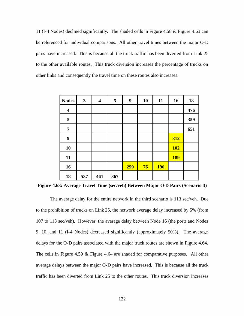
122
11 (I-4 Nodes) declined significantly. The shaded cells in Figure 4.58 & Figure 4.63 can
be referenced for individual comparisons. All other travel times between the major O-D
pairs have increased. This is because all the truck traffic has been diverted from Link 25
to the other available routes. This truck diversion increases the percentage of trucks on
other links and consequently the travel time on these routes also increases.
Nodes 3 4 5 9 10 11 16 18
4 476
5 359
7 651
9 312
10 102
11 189
16 299 76 196
18 537 461 367 Figure 4.63: Average Travel Time (sec/veh) Between Major O-D Pairs (Scenario 3)
The average delay for the entire network in the third scenario is 113 sec/veh. Due
to the prohibition of trucks on Link 25, the network average delay increased by 5% (from
107 to 113 sec/veh). However, the average delay between Node 16 (the port) and Nodes
9, 10, and 11 (I-4 Nodes) decreased significantly (approximately 50%). The average
delays for the O-D pairs associated with the major truck routes are shown in Figure 4.64.
The cells in Figure 4.59 & Figure 4.64 are shaded for comparative purposes. All other
average delays between the major O-D pairs have increased. This is because all the truck
traffic has been diverted from Link 25 to the other routes. This truck diversion increases
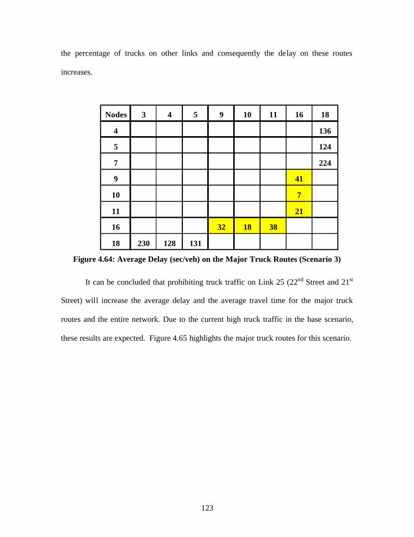
123
the percentage of trucks on other links and consequently the delay on these routes
increases.
Nodes 3 4 5 9 10 11 16 18
4 136
5 124
7 224
9 41
10 7
11 21
16 32 18 38
18 230 128 131 Figure 4.64: Average Delay (sec/veh) on the Major Truck Routes (Scenario 3)
It can be concluded that prohibiting truck traffic on Link 25 (22nd Street and 21st
Street) will increase the average delay and the average travel time for the major truck
routes and the entire network. Due to the current high truck traffic in the base scenario,
these results are expected. Figure 4.65 highlights the major truck routes for this scenario.

124
SR 676
SR 41
I-4
22nd St
N-18
N-1
N-16
60th St.
Figure 4.65: Major Truck Routes on the Port of Tampa Road Network (Scenario 3)
4.5.4 Scenario 4
The fourth scenario evaluates the network using the same measures of
effectiveness (average travel time and average delay) for an incident occurrence on Link
25 (22nd Street). Link 25 was reduced from two lanes to one for 22nd Street north of the
port (Node 16). One lane on 22nd Street would be blocked due to the incident. No other
modifications to the geometry or the traffic operation parameters were done to the Port of
Tampa road network.
The average travel time for the entire network is 397 sec/veh. See Appendix O,
Table O. 4 for average travel times and average delays for each link. The average travel
time for the entire network increased from 329 to 397 sec/veh (17% increase). The
average travel times between the major O-D pairs are shown in Figure 4.66. The average
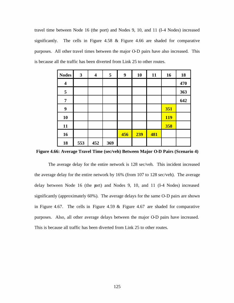
125
travel time between Node 16 (the port) and Nodes 9, 10, and 11 (I-4 Nodes) increased
significantly. The cells in Figure 4.58 & Figure 4.66 are shaded for comparative
purposes. All other travel times between the major O-D pairs have also increased. This
is because all the traffic has been diverted from Link 25 to other routes.
Nodes 3 4 5 9 10 11 16 18
4 470
5 363
7 642
9 351
10 119
11 358
16 456 239 481
18 553 452 369 Figure 4.66: Average Travel Time (sec/veh) Between Major O-D Pairs (Scenario 4)
The average delay for the entire network is 128 sec/veh. This incident increased
the average delay for the entire network by 16% (from 107 to 128 sec/veh). The average
delay between Node 16 (the port) and Nodes 9, 10, and 11 (I-4 Nodes) increased
significantly (approximately 60%). The average delays for the same O-D pairs are shown
in Figure 4.67. The cells in Figure 4.59 & Figure 4.67 are shaded for comparative
purposes. Also, all other average delays between the major O-D pairs have increased.
This is because all traffic has been diverted from Link 25 to other routes.

126
Nodes 3 4 5 9 10 11 16 18
4 156
5 120
7 243
9 47
10 42
11 61
16 63 49 84
18 243 138 126 Figure 4.67: Average Delay (sec/veh) on the Major Truck Routes (Scenario 4)
It can be concluded that blocking one lane of 22nd Street for the entire traffic will
increase the average delay and the average travel time significantly for both the major
truck routes and for the entire network. This is expected considering 22nd St. (Link 25)
carries an estimated vehicular volume of 1,000 vehicles during the peak hour. Figure
4.68 highlights the major truck routes for this scenario.

127
SR 676
SR 41
I-4
22nd St
N-18
N-1
N-16
60th St.
Figure 4.68: Major Truck Routes on the Port of Tampa Road Network (Scenario 4)
128
5. TRANSFERABILITY
5.1 Develop Route Assignment Model
The results from the Port of Tampa route assignment modeling provided
supporting conclusions that VISSIM is easier to use for building a road network.
Therefore, VISSIM was selected to test the transferability of the methodology developed
with the Port of Tampa. The same general methodology steps for modeling the trucks
generated by the Port of Tampa’s freight activity were followed for Port Canaveral.
5.1.1 Port Canaveral Network Definition
The road network connecting to Port Canaveral has been defined based on
FDOT’s 1999 Traffic Data CD and observations of the surrounding area roads that can
accommodate heavy trucks. Table 5.1 lists the data extracted from the FDOT data CD.
A number of trips were made to the Cape Canaveral area to investigate the network.
Figure 5.1 is a map of the surrounding area.

129
Link # Start Node End Node* FDOT Site # AADT K-Factor D-Factor T-Factor1 node 1 node 4 359 48500 10.31 53.65 5.879 node 1 - 362 26500 10.31 53.65 4.758 node 1 - 360 38000 10.31 53.65 5.872 node 1 node 2 361 37000 10.31 53.65 2.562 node 1 node 2 280 32500 10.31 53.65 5.210 node 2 node 7 13 39000 10.31 53.65 1.6110 node 2 node 7 1007 31500 10.31 53.65 2.6410 node 2 node 7 5153 26000 10.31 53.65 1.613 node 3 node 2 5119 32500 10.31 53.65 1.613 node 3 node 2 5069 16500 10.31 99.99 1.613 node 3 node 2 5071 24500 10.31 99.99 1.6112 node 3 - 353 36000 10.31 53.65 4.535 node 3 node 5 5068 26000 10.31 53.65 13.975 node 3 node 5 78 21000 10.31 53.65 13.975 node 3 node 5 80 22000 10.31 53.65 13.9714 node 5 - 365 55500 10.64 57.14 20.4516 node 5 - 385 13300 10.31 53.65 13.976 node 5 node 6 366 42000 10.64 57.14 21.336 node 5 node 6 368 42500 10.64 57.14 21.2315 node 6 - 399 16900 10.31 53.65 13.7613 node 6 - 401 33000 10.64 57.14 21.237 node 6 node 4 400 19600 10.31 53.65 13.767 node 6 node 4 377 26000 10.31 53.65 5.1611 node 4 - 403 33500 10.31 53.65 4.534 node 4 node 3 187 39000 10.31 53.65 4.534 node 4 node 3 5064 35000 10.31 53.65 4.534 node 4 node 3 5124 29000 10.31 53.65 4.534 node 4 node 3 5125 26500 10.31 53.65 3.3417 node 7 - 5115 40500 10.31 53.65 5.8717 node 7 - 135 38500 10.31 53.65 5.8717 node 7 - 5182 38500 10.31 53.65 5.8717 node 7 - 5181 26500 10.31 53.65 5.8717 node 7 - 354 28000 10.31 53.65 5.87* the "-" indicates exit from the network.
K-Factor: ratio between the peak hourly volume and daily volume.
D-Factor: directional factor
T-Factor: converts a truck volume to the relevant total traffic volume.
Table 5.1: 1999 FDOT Traffic CD Data for the Port Canaveral Network

130
Figure 5.1: Cape Canaveral Area Map
Figure 5.2 is a diagram of the network. Table 5.2 lists the links and nodes for the
Port Canaveral network with their corresponding descriptions. Most of the links are
interstate highways or state roads that have high capacity due to their geometric features.
No other major routes used by the trucks transporting freight to and from the port have
been identified. Internal nodes are locations on the identified network where traffic can
travel from one link to another. These are road intersections or interchanges. External
nodes are the origin-destination points for the network and make up the Origin-
Destination (O-D) matrix used as input to the computer simulation model. An external
node can be a special generator such as a port, an intersection, interchange, or a
termination point on a network link that extends outside the selected network boundary.
Due to the difference in complexity between Tampa and Cape Canaveral the level of
detail for Tampa was much greater than the Port Canaveral road network. Furthermore,
Orlando

131
the Cape Canaveral area is less urbanized than Tampa thus attributing to the differences
in the defined network. These differences are a desired component for testing the
transferability of the methodology to a different port network.
Figure 5.2: Port Canaveral Truck Route Network
Orlando
West SR 520

132
Link # Link Description Node #Internal Node Description
1 SR 528 (between SR 3 and US 1) 1 SR 528 and SR 32 SR 3 (between SR 528 and SR 520) 2 SR 520 and SR 33 SR 520 (between SR 3 and US 1) 3 SR 520 and US 14 US 1 (between SR 528 and SR 520) 4 SR 528 and US 15 SR 520 (between US 1 and I 95) 5 SR 520 and I 956 I 95 (between SR 528 and SR 520) 6 SR 528 and I 957 SR 528 (between Industry Rd and I 95) 7 SR 520 and SR A1A8 SR 528 (between Port Canaveral and SR 3) 8 SR 528 and Industry Rd9 SR 3 (North of SR 528)10 SR 520 (East of SR 3) External Nodes11 US 1 (North of SR 528) West SR 52012 US 1 (South of SR 528) South I-9513 I 95 (North of SR 528) North I-9514 I 95 (South of SR 520) South US 115 SR 528 (between Orlando and I 95) North US 116 SR 520 (West of I 95) South SR 317 SR A1A (North of SR 520) North SR 318 SR 528 (between US 1 and Industry Rd) South A1A19 Industry Rd (North of SR 528) Orlando20 SR 3 (South of SR 528) Port Canaveral21 SR A1A (South of SR 520) Industry Road
Table 5.2: Port Canaveral Network Links and Nodes
5.1.2 Port Canaveral Network Data Collection
Data supplied by the Brevard County Traffic Division and the City of Cocoa were
used with field data and observations to build the Port Canaveral network. The City of
Cocoa provided a minimal set of turning movement data and results from a couple of
local traffic studies.
Signal timing sheets were provided for eight intersections. These sheets
documented the green time allocated for each direction. They also included the
geometric features of each intersection. The geometric features included number of
lanes, left turn bays, right turn bays, and the configuration of the intersection (i.e. islands,
medians). Table 5.3 lists the data received from Brevard County by node number and

133
intersection. The date field is when the data was most recently updated, according to
Brevard County. All other data necessary for developing the model were obtained
through observations in the field.
In order to build the initial O-D matrix, the 1999 FDOT Traffic CD data was
utilized. Table 5.1 summarized the traffic data for the Port Canaveral network from the
FDOT Traffic CD. This traffic data combined with the link and node information was
the data used to build the initial model and begin the calibration.
Node Intersection Signal Timing Geometric Features Date Source
1 SR 3 & SR 528 WB Ramp Available Available Jul-01 Brevard County
1 SR 3 & SR 528 EB Ramp Available Available Jul-01 Brevard County
2 SR 3 & SR 520 Available Available Jan-02 Brevard County
3 US 1 & SR 520 Available Available May-00 Brevard County
4 US 1 & SR 528 WB Ramp Available Available May-00 Brevard County
4 US 1 & SR 528 EB Ramp Available Available May-00 Brevard County
5 SR 520 & I-95 SB Ramp Available Available May-00 Brevard County
5 SR 520 & I-95 NB Ramp Available Available May-00 Brevard County
Table 5.3: Brevard County Traffic Data Inventory
5.1.3 Port Canaveral Field Traffic Data Collection: Freight Terminals
Data collection began on September 20th, 2001 at the north and south freight
terminals and was completed at the end of March 2002. Figure 5.3 shows a layout of the
port area. The blue stars indicate the data collection locations for the truck counts at the
north and south freight terminals.

134
Figure 5.3: Port Canaveral Map
South Terminal
North Terminal
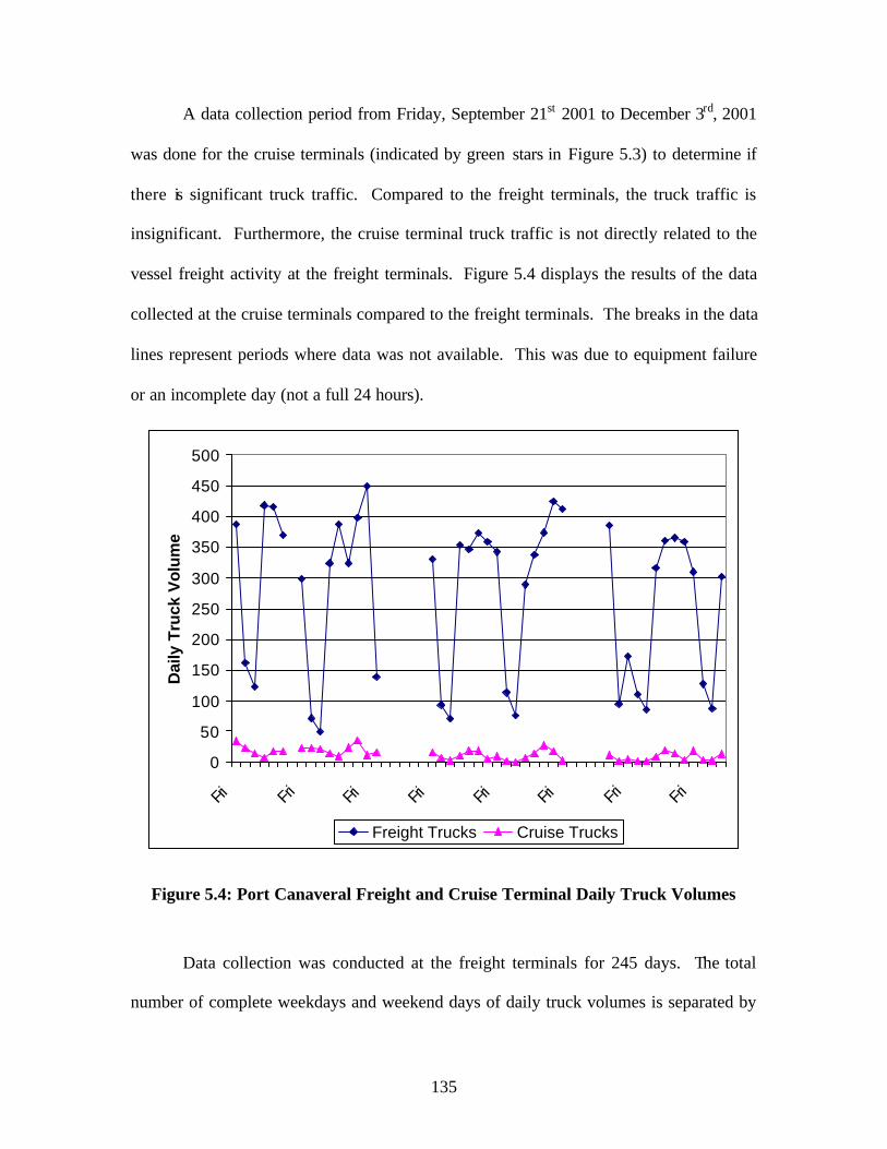
135
A data collection period from Friday, September 21st 2001 to December 3rd, 2001
was done for the cruise terminals (indicated by green stars in Figure 5.3) to determine if
there is significant truck traffic. Compared to the freight terminals, the truck traffic is
insignificant. Furthermore, the cruise terminal truck traffic is not directly related to the
vessel freight activity at the freight terminals. Figure 5.4 displays the results of the data
collected at the cruise terminals compared to the freight terminals. The breaks in the data
lines represent periods where data was not available. This was due to equipment failure
or an incomplete day (not a full 24 hours).
0
50
100
150
200
250
300
350
400
450
500
Fri Fri Fri Fri Fri Fri Fri Fri
Dai
ly T
ruck
Vol
ume
Freight Trucks Cruise Trucks
Figure 5.4: Port Canaveral Freight and Cruise Terminal Daily Truck Volumes
Data collection was conducted at the freight terminals for 245 days. The total
number of complete weekdays and weekend days of daily truck volumes is separated by

136
direction. 102 complete weekdays and 40 complete weekends have been collected for the
inbound direction and 90 complete weekdays and 35 complete weekends for the
outbound direction. These include both the North and South Terminals. A complete day
is considered any day when data for both locations was collected without errors for a 24-
hour period. A 24-hour period is from midnight (12:00 AM) of one day to the following
day. The Artificial Neural Network (ANN) truck trip generation port model is structured
with two separate internal models, one for inbound trucks and one for outbound trucks.
Table 5.4 details the collected data at each terminal by direction.
Terminal Location
Total Number of Days
Number of Week Days
Number of Weekend Days
Begin Date End Date
South – in 156 112 44 Sep 20, 2001 Mar 31, 2002 South – out 161 115 46 Sep 20, 2001 Mar 31, 2002 North – in 177 125 52 Sep 20, 2001 Mar 31, 2002 North - out 146 104 42 Sep 20, 2001 Mar 31, 2002
Table 5.4: Truck Count Data Inventory for Port Canaveral Freight Terminals
Figure 5.5 shows the trend of total inbound and outbound daily truck volumes for
the data collected from September 2001 through March 2002. The two adjacent low
points throughout the graph indicate the weekend days. The gap between the data is
when the data was incomplete. Initial comparison between the North and South
Terminals indicates the South Terminal has over 50% more trucks. From previous
discussions with port officials, these truck counts seem reasonable. Furthermore, the
increasing trend in truck volumes through March 2002 reflects the seasonal traffic
including the citrus products.

137
0
100
200
300
400
500
600
9/21/0
110/
5/01
10/19
/01
11/2/0
1
11/16
/01
11/30
/01
12/14
/01
12/28
/01
1/11/0
21/2
5/02
2/8/02
2/22/0
23/8
/02
3/22/0
2
Date
Dai
ly T
ruck
Vo
lum
e
Inbound Outbound
Figure 5.5: Port Canaveral Freight Terminal Daily Truck Volumes
5.1.4 Port Canaveral Field Traffic Data Collection: Road Network
The data collection locations on the Port Canaveral road network for use in
calibration and validation of the developed model were selected based on the necessity to
capture a significant portion of the truck traffic that are not local trips generated by the
freight operations at the port. A local trip is a trip generated by the port’s freight activity
but does not leave the Cape Canaveral area surrounding the network. An example of a
local trip would be between the port and the Rinker Cement facility on Industry Road
(Link #19). This was concluded through communications with the Canaveral Port
Authority contacts and local tenants handling the freight operations at the port.

138
The selected locations capture the truck traffic generated by the port’s freight
activity that travel on major highways linked to the defined network that are utilized for
long distance interstate and intrastate travel. Interstate 95 (I-95) and State Road 528 (SR
528) were identified as major truck routes. Port generated trucks travel these routes to
carry freight imported and/or exported at the port by vessel to areas outside the local
Cape Canaveral road network.
Industry Road has some truck activity due to the large Rinker Cement facility but
any truck traffic generated from Rinker’s port facilities are captured by the selected data
collection locations. US 1 was previously considered because of the rail terminal north
of SR 528. However, interviews with the operators have determined that truck volumes
generated by the port activity are local trips between the rail terminal and the port.
Furthermore, truck traffic generated by port freight activity that also visits the rail
terminal is captured on the network by the new data collection locations. Though SR 520
does not carry any significant port generated truck traffic, it has been included as part of
the Port Canaveral modeled network for purposes of Intelligent Transportation Systems
(ITS) applications. SR 520 is a viable alternate truck route that can be utilized in the
event of a disruption to the SR 528 route. Figure 5.2 previously displayed is a diagram of
the network and Table 5.2 lists the links and nodes for the Port Canaveral network with
their corresponding descriptions.
The network data collection sites, which were used for the calibration and
validation of the Port Canaveral network model, were located at node number 6 and link
numbers 7 and 8. A total of eight sites were utilized for the network modeling calibration
and validation along with the freight terminal traffic volume data. These eight sites are

139
described in Table 5.5 and identified on the network in Figure 5.6. Traffic on SR 528
(Link #15) that is originating from or destined to Central Florida and the Orlando area
was calculated from sites N6-ONa, N6-ONb and L7E for eastbound traffic and from sites
N6-OFa, N6-OFb and L7W for westbound traffic.
Site ID Description Link # Node #N6-Onb I-95 southbound off-ramp (SR 528 on-ramp) N/A 6N6-Ona I-95 northbound off-ramp (SR 528 on-ramp) N/A 6L7E SR 528 eastbound (near I-95) 7 N/AL8E SR 528 eastbound (near port) 8 N/AL8W SR 528 westbound (near port) 8 N/AL7W SR 528 westbound (near I-95) 7 N/AN6-Ofa I-95 northbound on-ramp (SR 528 off-ramp) N/A 6N6-Ofb I-95 southbound on-ramp (SR 528 off-ramp) N/A 6N/A: not applicable to this Site ID (can only be a link or node)
Table 5.5: Network Data Collection Site ID and Description
Figure 5.6: Data Collection Sites (Site IDs) on Port Canaveral Truck Route Network
P (freight terminals)
L7W
L7E
L8W
L8E N6-ONb
N6-ONa
N6-OFa N6-OFb
140
5.1.5 Port Canaveral Data Collection: Vessel Freight Data
Due to the fact that Port Canaveral was not part of Phase II, a truck trip generation
model was not previously developed for this port. Therefore, not only was it necessary to
have historical data for forecasting future estimates of vessel freight activity, current
freight data was also necessary. This current data was utilized to build an Artificial
Neural Network (ANN) truck trip generation model for Port Canaveral following the
same methodology developed in Phase II of this study (11).
Current freight data has been received for the months corresponding to the freight
terminal truck counts. Daily vessel freight records have been received from August 30,
2001 to April 15, 2002. These include 273 individual vessel records. The list of
commodity types and corresponding unit of measure presently being handled at the port
are listed in Table 5.6. This vessel freight data was used as input for building the Port
Canaveral ANN truck trip generation model. Figure 5.7 and Figure 5.8 display the
significant commodities for both imported and exported freight. It is important to
recognize significant commodity types because changes in them can significantly
influence the number of trucks at the port.

141
Exports ImportsCommodity Unit Type Commodity Unit TypeDiesel BBLS #6 Oil BBLS20' Container (Empty) Each 64 Grade BBLS20' Container (Loaded) Each AC-30 BBLS20' Tank Containers (Loaded) Each Diesel BBLSCars/Boats Tons Oil BBLSCitrus Tons Prem Gas BBLSGen'l Misc Tons Reg.Unl. Gas BBLSPCS Equipment Tons Sp.Unl. Gas BBLSPickup Tons Spug BBLSSand Tons Unknown BBLSSS Juice Tons Lumber BDFTTruck/Trailers Tons 20' Container (Empty) EachTrucks Tons 20' Container (Unloaded) EachTrucks, Etc Tons Accomm. Units TonsVehicles Tons Bagged Cement Tons
Cement TonsEmpty Bins TonsEmpty Drums/Bins TonsGen'l Misc TonsHooper TonsNewsprint TonsPumice TonsRebar TonsSalt TonsScrap Steel TonsTreatment Plant TonsWrapper & Headers Tons
Table 5.6: Port Canaveral Commodity Types

142
16,277 34,513 10,884 29,315
1,461,423
475,160
150,942124,004
0
200,000
400,000
600,000
800,000
1,000,000
1,200,000
1,400,000
1,600,000
Petrole
umCem
ent
Newsp
rint Salt
Lumber
Slate/G
ran Sa
nd Drywall
Rebar/
Granite
Commodity
To
nn
age
Imports
Figure 5.7: Port Canaveral Significant Imported Commodities
31,676 45,6224,691
672,308
70,447
0
100,000
200,000
300,000
400,000
500,000
600,000
700,000
800,000
Concentrate SS juice Citrus Cars/Trucks GeneralCargo
Commodity
Tonn
age
Exports
Figure 5.8: Port Canaveral Significant Exported Commodities

143
5.1.6 Port Canaveral Network Coding: VISSIM
The data obtained from FDOT, the local public agencies and the field was used to
code the network in VISSIM. The same process outlined for the Port of Tampa model
was followed. Once the initial VISSIM model was coded, the traffic counts were utilized
for the calibration and validation.
5.2 Route Assignment Model Calibration
5.2.1 Port Canaveral Network Model Calibration: VISSIM
The same methodology for calibration and validation developed for the Port of
Tampa and successfully applied was followed for Port Canaveral network modeling. A
cordon line was drawn around the port indicated by a green line in Figure 5.9. This
cordon line was used to select the initial links for tracking the total vehicles in and out of
the port and also confirmed selection of the master links utilized in the calibration and
validation steps. The links cut by the cordon line were used in determining the initial O-
D matrix. Then, the master links were used to complete the calibration.
Due to Port Canaveral’s limited access routes, only three master links were
identified for the port located on SR 528 (Bee Line Toll Road). Figure 5.9 shows a Cape
Canaveral area map with the cordon line and the master links. The master links are Links
#7, #8, and #15. Though SR 520 to A1A is a possible access route to the port, it was not
selected as a master link due to the fact that virtually no heavy trucks generated by the
port’s freight activity use this route for travel. It is a possible alternate route that could be
used with ITS applications but not applicable for the present calibration. This was
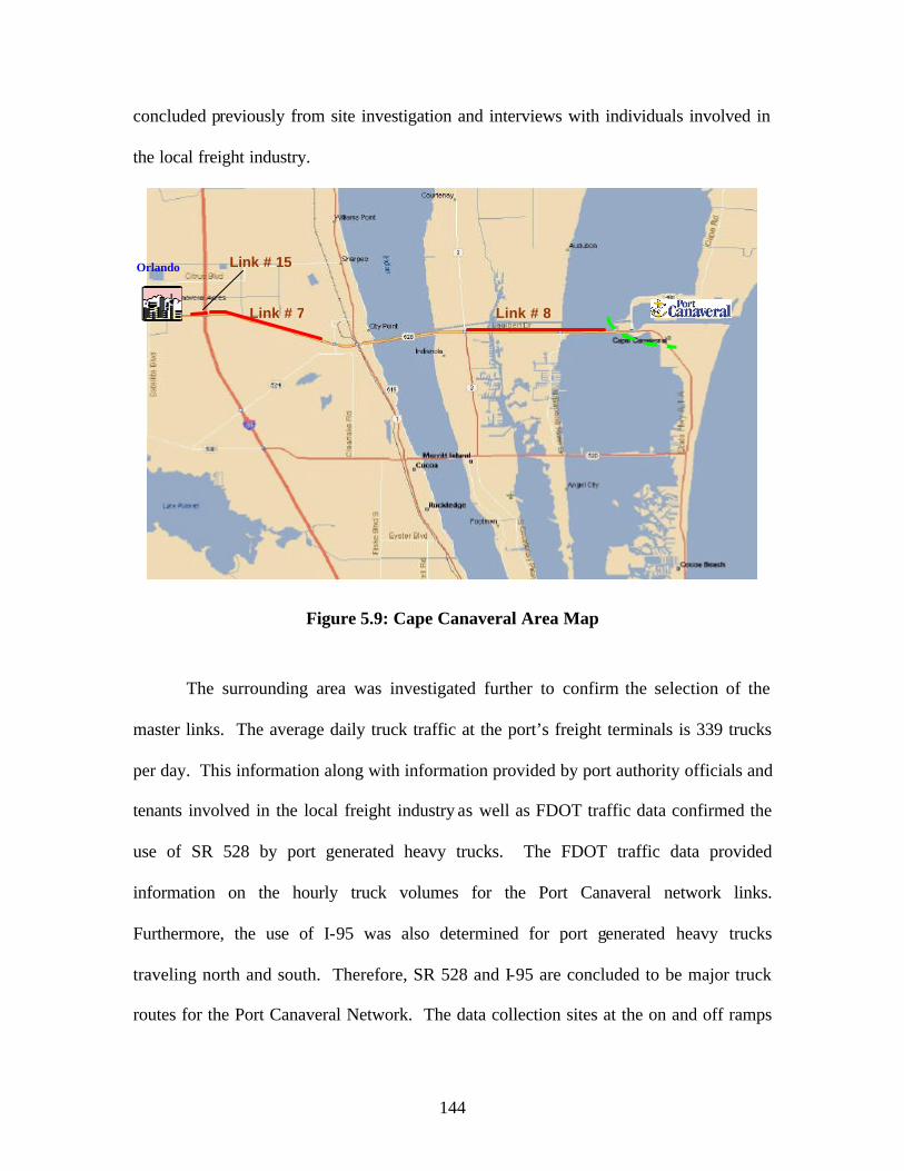
144
concluded previously from site investigation and interviews with individuals involved in
the local freight industry.
Figure 5.9: Cape Canaveral Area Map
The surrounding area was investigated further to confirm the selection of the
master links. The average daily truck traffic at the port’s freight terminals is 339 trucks
per day. This information along with information provided by port authority officials and
tenants involved in the local freight industry as well as FDOT traffic data confirmed the
use of SR 528 by port generated heavy trucks. The FDOT traffic data provided
information on the hourly truck volumes for the Port Canaveral network links.
Furthermore, the use of I-95 was also determined for port generated heavy trucks
traveling north and south. Therefore, SR 528 and I-95 are concluded to be major truck
routes for the Port Canaveral Network. The data collection sites at the on and off ramps
Orlando
Link # 7 Link # 8
Link # 15

145
between SR 528 and I-95 provided the necessary data for successfully modeling the
network and determining the number of heavy trucks generated by the port using I-95.
Calibration Using FDOT Data
The initial O-D matrix concluded using the FDOT data is displayed in Figure
5.10. The O-D matrix field titles of Figure 5.10 indicate the external nodes of the
network that are indicated in Figure 5.2, previously displayed. The Port freight terminals
identify the freight terminal traffic volume in the O-D matrix. The traffic at the port not
directly associated with the freight activity is included in the matrix as local port traffic.
Local port traffic is all traffic entering and leaving the port on George King Blvd. and SR
401 excluding the port freight terminal traffic volumes at the sites indicated previously in
Figure 5.3. The FDOT data used for this initial calibration is displayed in Table 5.7. No
FDOT data was available for the selected Master Link #15. The PM peak hour (4:00-
5:00) was found to be highest and used for the model development.
LT S1 U1 I1 R2 U2 S2 A2 IN O I2 P
LT 0 350 350 600 10 150 150 1000 5 300 400 5 3320
S1 150 0 10 10 40 10 1200 100 5 100 10 30 1665
U1 150 10 0 10 50 1100 10 100 5 100 10 30 1575
I1 250 10 10 0 300 10 10 40 5 350 1000 40 2025
R2 10 40 10 800 0 100 100 300 5 10 500 5 1880
U2 100 200 900 10 200 0 10 300 5 50 10 10 1795
S2 100 400 10 10 100 10 0 340 5 50 10 10 1045
A2 600 300 200 250 500 400 200 0 5 10 500 10 2975
IN 30 10 10 10 10 10 10 10 0 10 10 30 150
O 150 200 200 400 10 175 175 10 20 0 400 30 1770
I2 100 10 10 1000 400 10 10 500 5 250 0 10 2305
P 5 80 80 200 10 40 40 20 30 50 20 0 575
1645 1610 1790 3300 1630 2015 1915 2720 95 1280 2870 210
South US 1
South SR 3
South A1A
Local Port Traffic
North SR 3
North US 1
North I-95
Orlando
South I-95
Port (Freight Term.)
Att.
Prod.Calibration O/D
Industry Road Orlando
South I-95
Port (Freight Term.)
Industry Road
West SR 520
Local Port
Traffic
North SR 3
North US 1
North I-95
West SR 520
South US 1
South SR 3
South A1A
Figure 5.10: Initial Port Canaveral O-D Matrix

146
Site ID Link # Description Direction Peak Hour Traffic VolumeL7E 7 SR 538 eastbound (just east of I-95 ramps) Inbound 937L8E 8 SR 528 eastbound (near port) Inbound 1816L8W 8 SR 528 westbound (near port) Outbound 2102L7W 7 SR 528 westbound (just east of I-95 ramps) Outbound 1084
Table 5.7: FDOT PM Peak Hour Traffic Volumes (Calibration Data)
Calibration Using Field Data
Once the initial O-D matrix was determined, calibration continued using field data
including data collected for the identified master links (Links #7, #8, and #15). Link #15
is the through traffic on SR 528 just west of I-95. It does not include the SR 528
eastbound traffic that exits SR 528 west of I-95 or the SR 528 westbound traffic that
enters SR 528 west of I-95. The field data set spans the time period from April 13, 2002
through May 10, 2002. Not all days of data collection were used due to incomplete data
sets. Incomplete data sets were days/time periods when the tubes were damaged or a
malfunction in the classifier or equipment.
Table 5.8 summarizes the inventory of data collected by location. This table
denotes the inventory of successful days for data collection. Unsuccessful days include
events when the tubes were damaged or there was a malfunction in the classifier or
equipment. This initial data set along with the initial O-D matrix using the FDOT traffic
CD data provides the information for determining a revised origin-destination (O-D)
matrix for the network modeling.

147
Site ID
Total Number of Days Begin Date End Date
N6-Onb 38 April 13, 2002 June 11, 2002N6-Ona 42 April 13, 2002 June 11, 2002L7E 35 April 13, 2002 June 11, 2002L8E 27 April 13, 2002 June 11, 2002L8W 36 April 13, 2002 June 11, 2002L7W 37 April 13, 2002 June 11, 2002N6-Ofa 39 April 13, 2002 June 11, 2002N6-Ofb 41 April 13, 2002 June 11, 2002
Table 5.8: Truck Count Data Inventory for Port Canaveral Network
From the field data inventory as displayed in Table 5.8, the average PM peak hour
traffic volumes were computed. The PM peak was concluded after analyzing the hourly
traffic volumes collected from the field traffic counters. The data used for calibration are
included in Table 5.9. Table 5.9 displays the total vehicular volume including heavy
trucks because VISSIM requires total number of all vehicles on the network for
simulation.
Once the model is calibrated and validated, the heavy truck volumes generated by
the port’s freight activity is determined from the total traffic volume results. From
Scheffe’s statistical test between weekdays, it was determined at the 95% confidence
level that no significant difference between days of the week exists. The results of this
test are provided in Appendix P. Therefore, the hourly traffic volume for the PM peak at
each field data collection site was used to determine an average value.
Figure 5.11 displays a diagram of the network with the data collection sites
identified including Site ID. The master links (denoted with blue) display significant
truck volumes. For Link 7, the average number of trucks per day was 663 eastbound and

148
881 westbound. For Link 8, the average number of trucks per day was 703 eastbound
and 750 westbound. The average peak hour traffic volume for the freight terminals at the
port during the study period was 320 vph inbound and 620 vph for the outbound.
Site ID Link # Description Direction Peak Hour Traffic VolumeL15E 15 SR 538 eastbound (just west of I-95 ramps) Inbound 513L7E 7 SR 538 eastbound (just east of I-95 ramps) Inbound 833L8E 8 SR 528 eastbound (near port) Inbound 977L8W 8 SR 528 westbound (near port) Outbound 2333L7W 7 SR 528 westbound (just east of I-95 ramps) Outbound 1221L15W 15 SR 528 westbound (just west of I-95 ramps) Outbound 587
Table 5.9: Port Canaveral Network Field Data (Calibration)
Figure 5.11: Calibration Data (Site IDs) on Port Canaveral Truck Route Network
The traffic data collected at Port Canaveral’s north and south freight terminals
were used for the input traffic volumes of the network model for the port node of the O-D
matrix. This traffic volume represents traffic generated from the activity at the port’s
freight terminals. Table 5.10 displays this data.
P L7W
L7E
L8W
L8E L15E
L15W

149
Location Inbound OutboundFreight Terminals 320 620
Table 5.10: Average PM Peak Hour Traffic Volume
After 35 iterations were performed for the developed network model, the final O-
D matrix was concluded. The final calibrated O-D matrix for the Port Canaveral road
network is displayed in Figure 5.12. The calibration results compared to the field data
are shown in Table 5.11. As previously done for the Port of Tampa, the O-D matrix was
used to conclude the number of trucks on the Port Canaveral network links. The O-D
pair volumes are used to calculate the number of trucks from the known percentages of
trucks on each of the network links. Table 5.11 shows the field traffic volumes and the
absolute percent error between the simulated and field traffic volumes for the master
links.
100% ∗−
=Field
SimulatedFieldError
The absolute percent error for every master link is less than 5%. This low percent error
provides concluding evidence that the final O-D matrix (Figure 5.12) represents the real
world (existing conditions) for the Port Canaveral road network. Figure 5.13 is a
graphical representation comparing the field and VISSIM Model results for each of the
data collection sites.
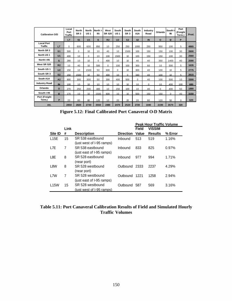
150
LT S1 U1 I1 R2 U2 S2 A2 IN O I2 P
LT 0 600 600 850 10 250 250 1000 250 950 100 5 4865
S1 500 0 10 10 40 10 1500 100 150 150 100 30 2600
U1 400 10 0 10 100 1500 10 100 150 150 100 30 2560
I1 280 10 10 0 400 10 10 40 40 350 1400 40 2590
R2 10 40 10 500 0 100 100 300 60 10 500 5 1635
U2 150 10 1500 50 600 0 10 300 40 100 10 5 2775
S2 150 1500 10 50 400 10 0 340 40 100 10 5 2615
A2 800 300 300 50 300 400 500 0 40 100 500 10 3300
IN 100 10 10 10 10 10 10 10 0 10 400 100 680
O 270 250 200 400 10 150 100 10 40 0 400 50 1880
I2 170 10 10 1500 600 10 10 500 150 150 0 40 3150
P 20 80 80 120 10 20 20 20 80 120 50 0 620
2850 2820 2740 3550 2480 2470 2520 2720 1040 2190 3570 320
Local Port
Traffic
North SR 3
North US 1
North I-95
West SR 520
South US 1
South SR 3
South A1A Prod.Calibration O/D
Industry Road
OrlandoSouth I-
95
Port (Freight Term.)
Industry Road
West SR 520
Orlando
South I-95
Port (Freight Term.)
Att.
South US 1
South SR 3
South A1A
Local Port Traffic
North SR 3
North US 1
North I-95
Figure 5.12: Final Calibrated Port Canaveral O-D Matrix
Peak Hour Traffic Volume
Site IDLink # Description Direction
Field Value
VISSIM Results % Error
L15E 15 SR 538 eastbound Inbound 513 519 1.16%(just west of I-95 ramps)
L7E 7 SR 538 eastbound Inbound 833 825 0.97%(just east of I-95 ramps)
L8E 8 SR 528 eastbound Inbound 977 994 1.71%(near port)
L8W 8 SR 528 westbound Outbound 2333 2237 4.29%(near port)
L7W 7 SR 528 westbound Outbound 1221 1258 2.94%(just east of I-95 ramps)
L15W 15 SR 528 westbound Outbound 587 569 3.16%(just west of I-95 ramps)
Table 5.11: Port Canaveral Calibration Results of Field and Simulated Hourly Traffic Volumes

151
0
500
1000
1500
2000
2500
L15E L7E L8E L8W L7W L15W
Site ID
Pea
k H
ou
r T
raff
ic V
olu
me
FieldVISSIM
Figure 5.13: Port Canaveral Calibration Results of Field and Simulated Hourly Traffic Volumes
5.3 Route Assignment Model Validation
5.3.1 Port Canaveral Network Model Validation: VISSIM The same steps outlined for the Port of Tampa used to validate the calibrated
network model were followed for the Port Canaveral calibrated network model. Eleven
days of field data collection were used for the validation. The validation data set is
shown in Table 5.12. This data is also the peak hour total traffic volumes including the

152
heavy truck volumes in vehicles per hour (vph). The inbound direction is eastbound and
the outbound direction is westbound (denoted in Site ID by E or W). The corresponding
peak hour total traffic volumes for the freight terminal locations (port node) are displayed
in Table 5.13.
Site IDDay # Date Direction L15E L7E L8E L8W L7W L15W1 29-Apr-02 Inbound 459 758 929 -- -- --
Outbound -- -- -- 2197 1120 5692 30-Apr-02 Inbound 473 776 844 -- -- --
Outbound -- -- -- 2347 1183 5913 1-May-02 Inbound 484 792 891 -- -- --
Outbound -- -- -- 2314 1148 5914 2-May-02 Inbound 462 763 940 -- -- --
Outbound -- -- -- 2361 1181 5855 3-May-02 Inbound 493 842 969 -- -- --
Outbound -- -- -- 2070 1197 6626 13-May-02 Inbound 437 724 837 -- -- --
Outbound -- -- -- 2007 1079 5577 14-May-02 Inbound 442 728 831 -- -- --
Outbound -- -- -- 2092 1052 4988 15-May-02 Inbound 495 812 905 -- -- --
Outbound -- -- -- 2216 1135 5509 28-May-02 Inbound 449 809 858 -- -- --
Outbound -- -- -- 2032 1080 55010 6-Jun-02 Inbound 516 850 885 -- -- --
Outbound -- -- -- 2387 1193 56811 10-Jun-02 Inbound 461 773 881 -- -- --
Outbound -- -- -- 2022 1258 692-- denotes the direction not applicable (locations are eastbound or westbound)
Table 5.12: Port Canaveral Network Field Data in vph (Validation)

153
Day # Date Direction
Hourly Traffic Volume
Hourly Truck Volume
1 29-Apr-02 Inbound 270 27Outbound 504 50
2 30-Apr-02 Inbound 262 26Outbound 552 55
3 1-May-02 Inbound 314 31Outbound 622 62
4 2-May-02 Inbound 375 38Outbound 616 62
5 3-May-02 Inbound 398 40Outbound 595 60
6 13-May-02 Inbound 288 29Outbound 477 48
7 14-May-02 Inbound 306 31Outbound 476 48
8 15-May-02 Inbound 254 25Outbound 541 54
9 28-May-02 Inbound 281 28Outbound 517 52
10 6-Jun-02 Inbound 339 34Outbound 583 58
11 10-Jun-02 Inbound 271 27Outbound 484 48
Table 5.13: Port Canaveral Freight Terminal Data in vph (Validation)
Once the model was run for each of the validation days using the Port Canaveral
Freight Terminal total traffic volumes as input to VISSIM, the results of each model run
were summarized. The resulting truck volumes for SR 528 are displayed in Table 5.14.
A graphical representation comparing these data is shown in Figure 5.14 through Figure
5.19. The Port Canaveral VISSIM model results were compared to the field data. Figure
5.14 through Figure 5.19 provide the graphs for the visual inspection.

154
LocationSR 528 (Link # 7)* SR 528 (Link # 8)* SR 528 (Link # 15)*
Day # Date Direction Field VISSIM Field VISSIM Field VISSIM1 29-Apr-02 Inbound 29 32 18 18 10 11
Outbound 55 61 42 42 37 362 30-Apr-02 Inbound 29 31 21 23 7 8
Outbound 52 55 43 40 26 243 1-May-02 Inbound 32 33 28 30 13 14
Outbound 52 58 49 48 29 274 2-May-02 Inbound 29 31 17 18 10 11
Outbound 46 50 53 50 14 145 3-May-02 Inbound 29 28 13 14 8 9
Outbound 51 53 41 44 24 216 13-May-02 Inbound 29 33 20 23 11 13
Outbound 59 67 106 116 39 387 14-May-02 Inbound 28 32 34 40 7 8
Outbound 48 57 115 120 14 158 15-May-02 Inbound 35 36 35 37 16 17
Outbound 55 61 124 123 28 299 28-May-02 Inbound 24 24 36 40 5 6
Outbound 42 48 130 140 20 2010 6-Jun-02 Inbound 26 25 20 22 9 9
Outbound 55 59 117 107 30 3011 10-Jun-02 Inbound 25 27 19 21 9 10
Outbound 67 67 111 121 44 35* denotes a master link
Table 5.14: Port Canaveral Validation Results of Field and Simulated Hourly Truck Volumes on SR 528

155
SR 528 eastbound (just east of I-95 ramps)
0
20
40
60
80
100
120
140
160
Day 1 Day 2 Day 3 Day 4 Day 5 Day 6 Day 7 Day 8 Day 9 Day 10 Day 11
Flo
w (
tru
cks/
ho
ur)
Field Vissim
Figure 5.14: Port Canaveral Validation Results of Field and Simulated Hourly Inbound Truck Volumes on SR 528 (Link #7)
SR 528 westbound (just west of I-95 ramps)
0
20
40
60
80
100
120
140
160
Day 1 Day 2 Day 3 Day 4 Day 5 Day 6 Day 7 Day 8 Day 9 Day 10 Day 11
Flow
(tr
ucks
/hou
r)
Field Vissim
Figure 5.15: Port Canaveral Validation Results of Field and Simulated Hourly Outbound Truck Volumes on SR 528 (Link #7)

156
SR 528 eastbound (near port)
0
20
40
60
80
100
120
140
160
Day 1 Day 2 Day 3 Day 4 Day 5 Day 6 Day 7 Day 8 Day 9 Day 10 Day 11
Flow
(tr
ucks
/hou
r)
Field Vissim
Figure 5.16: Port Canaveral Validation Results of Field and Simulated Hourly Inbound Truck Volumes on SR 528 (Link #8)
SR 528 westbound (near port)
0
20
40
60
80
100
120
140
160
Day 1 Day 2 Day 3 Day 4 Day 5 Day 6 Day 7 Day 8 Day 9 Day10
Day11
Flow
(tr
ucks
/hou
r)
Field Vissim
Figure 5.17: Port Canaveral Validation Results of Field and Simulated Hourly Outbound Truck Volumes on SR 528 (Link #8)

157
SR 528 eastbound (just west of I-95 ramps)
0
20
40
60
80
100
120
140
160
Day 1 Day 2 Day 3 Day 4 Day 5 Day 6 Day 7 Day 8 Day 9 Day 10 Day 11
Flo
w (
tru
cks/
ho
ur)
Field Vissim
Figure 5.18: Port Canaveral Validation Results of Field and Simulated Hourly Inbound Truck Volumes on SR 528 (Link #15)
SR 528 westbound (just west of I-95 ramps)
0
20
40
60
80
100
120
140
160
Day 1 Day 2 Day 3 Day 4 Day 5 Day 6 Day 7 Day 8 Day 9 Day 10 Day 11
Flo
w (
tru
cks/
ho
ur)
Field Vissim
Figure 5.19: Port Canaveral Validation Results of Field and Simulated Hourly Outbound Truck Volumes on SR 528 (Link #15)

158
After the visual inspection showed no major differences between the simulated
and the actual truck volumes on the master links, a statistical test was performed for each
of the master links using the Confidence Interval (C.I.) Statistical Test. Table 5.15
summarizes the C.I. calculations. Upper and lower limits of the confidence interval for
each of the master links include zero. Therefore, the C.I. test concludes there is no
significant difference between the simulated and actual truck volumes on the master
links.
Link Name (#) DirectionLower Limit
Upper Limit
Inbound -4.58 1.49Outbound -10.62 0.80Inbound -10.01 5.46Outbound -36.80 33.20Inbound -3.75 1.75Outbound -6.55 9.46
SR 528 (#7) near portSR 528 (#8) east of I-95 rampsSR 528 (#15) west of I-95 ramps
Table 5.15: Confidence Interval Limits for the Actual and VISSIM Simulated Truck Volumes
It can be concluded after conducting these two tests (visual inspection and C.I.
test) that the VISSIM Port Canaveral road network model replicates the existing
conditions of truck movements at the 95% confidence level. From the validation results
it is concluded that the O-D matrix in Figure 5.12 is the final O-D matrix and produces
simulation results representative of present traffic conditions. Furthermore, this network
model has been shown to perform accurately when utilizing traffic volumes generated by
Port Canaveral’s freight terminals, therefore this model can be used for short-term
forecasting. The conclusion for truck volumes on the routes identified as those traveled
by trucks that haul freight in and out of the port that is imported and exported by vessel
were detailed in Table 5.14. These are non- local truck trips.

159
For trucks destined to Port Canaveral generated by the port’s vessel freight
activity, 15.6% use SR 528 (eastbound), 12.5% use I-95 traveling northbound (coming
from areas south of SR 528) and 12.5% use I-95 traveling southbound (coming from
areas north of SR 528). For trucks originating from Port Canaveral, 19.4% use SR 528
(westbound), 19.4% use I-95 traveling northbound (going to areas north of SR 528) and
8.1% use I-95 traveling southbound (going to areas south of SR 528).
The network model has also captured port generated local truck trips. 12.9% of
the truck traffic generated by the port’s freight activity travel to Industry Road and 31.3%
of the trucks destined to the port are coming from Industry Road. This Industry Road
truck traffic is attributed to the large Rinker cement facility. Also, 12.9% of the trucks
were local trips to US1 and 9.4% of the truck trips to the port were from US1. This truck
traffic is attributed to the rail terminal located just northwest of SR 528.
5.4 Forecasting
In order to accurately forecast the number of port generated heavy trucks carrying
freight on the Port Canaveral road network, an accurate number of heavy trucks
generated by port vessel freight activity is essential. The Port Canaveral truck trip
generation model accurately produces this data. The model was developed by utilizing
the Artificial Neural Network modeling (ANN) methodology developed in Phase II (11).
These ANN models accurately produce the daily heavy truck movements inbound and
outbound for the seaports by using daily vessel freight data as input to the model. The

160
same basic methodology used to develop the ANN models for the ports of Palm Beach,
Everglades, Tampa and Jacksonville have been applied to Port Canaveral.
5.4.1 Port Canaveral ANN Model Development (Calibration)
The Port Canaveral ANN model was trained (calibrated) with data selected from
the inventory of data collected between Sept. 20, 2001 and March 31, 2002. This
inventory of data includes both vessel freight data provided by the Canaveral Port
Authority and heavy truck counts collected from the field. On March 7th, 2002, a
presentation was made to the port authority. One of the outcomes of this meeting verified
the accuracy of the daily truck counts taken from the field data. It was also stated that
presently, container traffic at the port is very minimal and there is no indication for the
near future that this would change. Due to the information provided by the port authority
and the insignificant amount of containerized freight, these records were excluded from
the model. Also, in order to more accurately model the trucks, the imported petroleum
products (barrels) were converted to tons with a conversion factor provided by the
Canaveral Port Authority and included with the imported tons. The ANN model data set
is provided in Table 5.16. Shaded records indicate weekend days.

161
Heavy Trucks Vessel Freight Data
Date Inbound OutboundImported Lumber
Imported Tons
Exported Tons
29-Sep-01 71 46 0 3136.8720 030-Sep-01 49 -- 0 361.8720 06-Oct-01 139 -- 0 3757.8720 07-Oct-01 39 -- 0 361.8720 011-Oct-01 355 318 187657 5284.7200 2813-Oct-01 112 -- 0 2487.9280 23614-Oct-01 -- 59 0 1250.9280 015-Oct-01 364 310 187657 3214.9280 23617-Oct-01 -- 326 187657 2566.2960 23619-Oct-01 352 -- 187657 5885.2960 26420-Oct-01 116 -- 0 5727.2960 24821-Oct-01 66 61 0 1465.2960 022-Oct-01 286 221 187657 5885.2960 2823-Oct-01 295 257 187657 5886.2960 2826-Oct-01 331 290 239882 6084.2400 28527-Oct-01 94 -- 0 5353.4240 25728-Oct-01 70 48 0 1103.4240 029-Oct-01 354 333 239882 5719.4240 48630-Oct-01 346 310 239882 5719.4240 48631-Oct-01 373 339 239882 6274.1600 4851-Nov-01 -- 343 239882 6798.9920 4853-Nov-01 114 89 0 3112.9920 2014-Nov-01 76 54 0 2182.9920 06-Nov-01 338 318 266190 4725.5520 2277-Nov-01 374 307 266190 4772.5520 2388-Nov-01 -- 360 266190 4772.5520 2279-Nov-01 -- 347 266190 3702.7040 22721-Nov-01 -- 339 266190 6116.1280 026-Nov-01 316 -- 304296 7860.0080 4027-Nov-01 -- 298 225000 7861.0080 4028-Nov-01 -- 350 225000 7861.0080 17229-Nov-01 359 326 225000 8304.0080 17230-Nov-01 310 329 225000 7749.2720 1721-Dec-01 128 133 0 6555.4400 1322-Dec-01 88 66 0 2197.4400 03-Dec-01 302 -- 225000 4438.9280 5044-Dec-01 274 -- 38106 4438.9280 5048-Dec-01 101 117 0 3217.3280 5439-Dec-01 -- 82 0 2267.3280 010-Dec-01 283 -- 38106 6535.3280 58413-Dec-01 -- 333 316595 6534.3280 58414-Dec-01 -- 291 316595 6609.3280 21015-Dec-01 -- 109 0 6503.3280 20916-Dec-01 58 58 0 2634.3280 0-- denotes 24 hour count not available
Table 5.16: Port Canaveral ANN Model Data
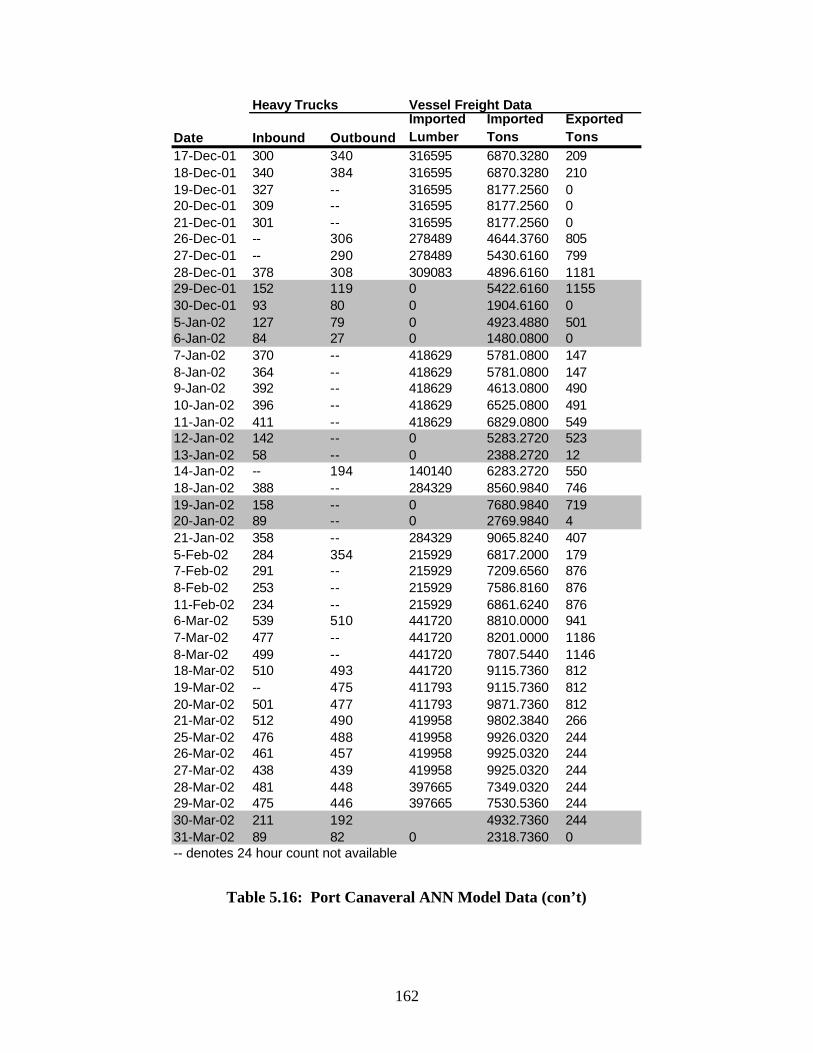
162
Heavy Trucks Vessel Freight Data
Date Inbound OutboundImported Lumber
Imported Tons
Exported Tons
17-Dec-01 300 340 316595 6870.3280 20918-Dec-01 340 384 316595 6870.3280 21019-Dec-01 327 -- 316595 8177.2560 020-Dec-01 309 -- 316595 8177.2560 021-Dec-01 301 -- 316595 8177.2560 026-Dec-01 -- 306 278489 4644.3760 80527-Dec-01 -- 290 278489 5430.6160 79928-Dec-01 378 308 309083 4896.6160 118129-Dec-01 152 119 0 5422.6160 115530-Dec-01 93 80 0 1904.6160 05-Jan-02 127 79 0 4923.4880 5016-Jan-02 84 27 0 1480.0800 07-Jan-02 370 -- 418629 5781.0800 1478-Jan-02 364 -- 418629 5781.0800 1479-Jan-02 392 -- 418629 4613.0800 49010-Jan-02 396 -- 418629 6525.0800 49111-Jan-02 411 -- 418629 6829.0800 54912-Jan-02 142 -- 0 5283.2720 52313-Jan-02 58 -- 0 2388.2720 1214-Jan-02 -- 194 140140 6283.2720 55018-Jan-02 388 -- 284329 8560.9840 74619-Jan-02 158 -- 0 7680.9840 71920-Jan-02 89 -- 0 2769.9840 421-Jan-02 358 -- 284329 9065.8240 4075-Feb-02 284 354 215929 6817.2000 1797-Feb-02 291 -- 215929 7209.6560 8768-Feb-02 253 -- 215929 7586.8160 87611-Feb-02 234 -- 215929 6861.6240 8766-Mar-02 539 510 441720 8810.0000 9417-Mar-02 477 -- 441720 8201.0000 11868-Mar-02 499 -- 441720 7807.5440 114618-Mar-02 510 493 441720 9115.7360 81219-Mar-02 -- 475 411793 9115.7360 81220-Mar-02 501 477 411793 9871.7360 81221-Mar-02 512 490 419958 9802.3840 26625-Mar-02 476 488 419958 9926.0320 24426-Mar-02 461 457 419958 9925.0320 24427-Mar-02 438 439 419958 9925.0320 24428-Mar-02 481 448 397665 7349.0320 24429-Mar-02 475 446 397665 7530.5360 24430-Mar-02 211 192 4932.7360 24431-Mar-02 89 82 0 2318.7360 0-- denotes 24 hour count not available
Table 5.16: Port Canaveral ANN Model Data (con’t)
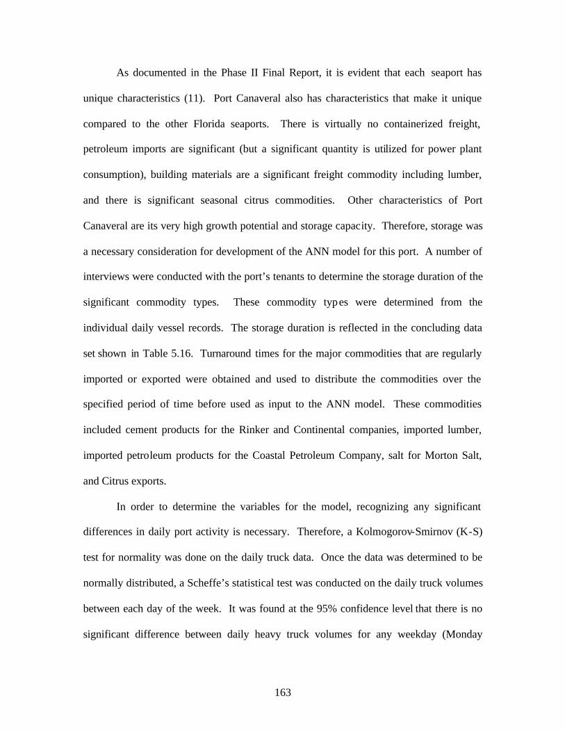
163
As documented in the Phase II Final Report, it is evident that each seaport has
unique characteristics (11). Port Canaveral also has characteristics that make it unique
compared to the other Florida seaports. There is virtually no containerized freight,
petroleum imports are significant (but a significant quantity is utilized for power plant
consumption), building materials are a significant freight commodity including lumber,
and there is significant seasonal citrus commodities. Other characteristics of Port
Canaveral are its very high growth potential and storage capacity. Therefore, storage was
a necessary consideration for development of the ANN model for this port. A number of
interviews were conducted with the port’s tenants to determine the storage duration of the
significant commodity types. These commodity types were determined from the
individual daily vessel records. The storage duration is reflected in the concluding data
set shown in Table 5.16. Turnaround times for the major commodities that are regularly
imported or exported were obtained and used to distribute the commodities over the
specified period of time before used as input to the ANN model. These commodities
included cement products for the Rinker and Continental companies, imported lumber,
imported petroleum products for the Coastal Petroleum Company, salt for Morton Salt,
and Citrus exports.
In order to determine the variables for the model, recognizing any significant
differences in daily port activity is necessary. Therefore, a Kolmogorov-Smirnov (K-S)
test for normality was done on the daily truck data. Once the data was determined to be
normally distributed, a Scheffe’s statistical test was conducted on the daily truck volumes
between each day of the week. It was found at the 95% confidence level that there is no
significant difference between daily heavy truck volumes for any weekday (Monday

164
through Friday). However, there was a significant difference between a weekday and a
weekend day. The results of this test can be seen in Appendix P. This concluded the
significance in the day of the week for model development. This information was also
useful in determining the structure of the model and the input data for calibration.
From regression analysis, the independent variables for the model were
concluded. The input variables for calibrating the Port Canaveral ANN model are listed
in Table 5.17 below.
Independent Variables Dependent VariablesImported Lumber (ImpBDFT) Inbound TrucksImported Tons* (ImpTons) Outbound TrucksExported Tons (ExpTons)Saturday (Sat)Sunday (Sun)* includes petroleum products converted to tons
Table 5.17: Input Variables for the Port Canaveral ANN Model
There were 81 records consisting of both independent and dependent variables
used in calibration. The independent variables basically consist of vessel freight data,
date and day of the week. The dependent variables are the daily inbound and outbound
heavy truck volumes and corresponding date. The final ANN model structure is shown
in Figure 5.20. The ANN model consists of an input layer, a hidden layer, and an output
layer. These layers are the components of the ANN model for computation. The hidden
layer is an additional internal model computation interval that performs a more detailed
analysis of the data.
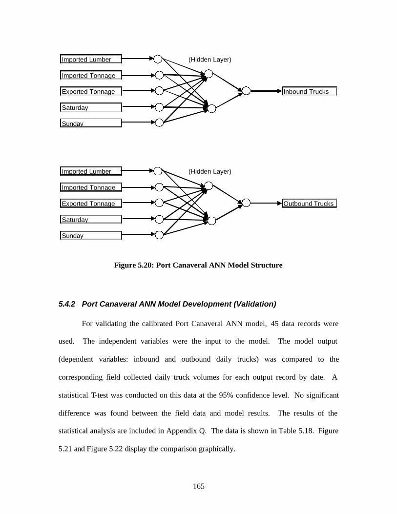
165
Imported Lumber (Hidden Layer)
Imported Tonnage
Exported Tonnage Inbound Trucks
Saturday
Sunday
Imported Lumber (Hidden Layer)
Imported Tonnage
Exported Tonnage Outbound Trucks
Saturday
Sunday
Figure 5.20: Port Canaveral ANN Model Structure
5.4.2 Port Canaveral ANN Model Development (Validation)
For validating the calibrated Port Canaveral ANN model, 45 data records were
used. The independent variables were the input to the model. The model output
(dependent variables: inbound and outbound daily trucks) was compared to the
corresponding field collected daily truck volumes for each output record by date. A
statistical T-test was conducted on this data at the 95% confidence level. No significant
difference was found between the field data and model results. The results of the
statistical analysis are included in Appendix Q. The data is shown in Table 5.18. Figure
5.21 and Figure 5.22 display the comparison graphically.

166
Inbound Trucks Outbound TrucksDate Field Model Date Field Model29-Sep-01 71 95 21-Oct-01 61 6430-Sep-01 49 47 22-Oct-01 221 31026-Oct-01 331 328 23-Oct-01 257 31027-Oct-01 94 139 26-Oct-01 290 34228-Oct-01 70 62 28-Oct-01 48 5929-Oct-01 354 332 29-Oct-01 333 31230-Oct-01 346 332 30-Oct-01 310 31231-Oct-01 373 340 31-Oct-01 339 30526-Nov-01 316 372 27-Nov-01 298 35418-Dec-01 340 374 28-Nov-01 350 35719-Dec-01 327 381 29-Nov-01 326 36320-Dec-01 309 381 30-Nov-01 329 35621-Dec-01 301 381 15-Dec-01 109 12428-Dec-01 378 329 16-Dec-01 58 8129-Dec-01 152 121 17-Dec-01 340 38430-Dec-01 93 78 18-Dec-01 384 38418-Jan-02 388 343 26-Dec-01 306 24219-Jan-02 158 130 27-Dec-01 290 24521-Jan-02 358 398 28-Dec-01 308 2538-Feb-02 253 301 29-Dec-01 119 13711-Feb-02 234 292 18-Mar-02 493 48818-Mar-02 510 43425-Mar-02 476 47026-Mar-02 461 470shaded cells denote weekends
Table 5.18: Port Canaveral ANN Model Validation Data
0
100
200
300
400
500
600
1 3 5 7 9 11 13 15 17 19 21 23
Record Number
Dai
ly T
ruck
Vo
lum
e
ActualModel
Figure 5.21: Port Canaveral ANN Model Validation Data (Inbound Trucks)

167
0
100
200
300
400
500
600
1 3 5 7 9 11 13 15 17 19 21
Record Number
Dai
ly T
ruck
Vo
lum
e
ActualModel
Figure 5.22: Port Canaveral ANN Model Validation Data (Outbound Trucks)
5.4.3 Port Canaveral ANN Model (Forecasting)
To obtain the necessary input for modeling the Port Canaveral road network to
determine future truck volumes, the Port Canaveral ANN model must first be executed.
From the historical vessel data provided by the Canaveral Port Authority, an Auto
Regression Integrated Moving Average (ARIMA) time series model was developed to
produce short-term forecasts of freight vessel data (11). This methodology was
previously developed in Phase II of this study.
The historical vessel data was available only as units of tons. The Canaveral Port
Authority provided 85 months of historical monthly vessel records. Table 5.19, which
displays the historical data used in forecasting the vessel data for the five years following,
lists the freight in the same variable groups used for the ANN model development.
Lumber was grouped in one field and all other general commodities were combined

168
under the imported or exported “tons” fields including petroleum products. Figure 5.23
and Figure 5.24 show the historical trends for this freight vessel data.

169
Imports Exports Imports ExportsDate Tons Lumber* Tons Date Tons Lumber* TonsOct-1994 130523 0 128264 Mar-1998 177944 632 88744Nov-1994 192686 1878 53303 Apr-1998 272988 2237 106531Dec-1994 190845 1597 82769 May-1998 258188 657 63198Jan-1995 135791 0 122553 Jun-1998 296760 4891 83977Feb-1995 253386 0 99961 Jul-1998 328203 637 104768Mar-1995 164250 2057 88155 Aug-1998 296254 640 97881Apr-1995 184706 2300 79360 Sep-1998 254025 3959 66495May-1995 137154 2461 74492 Oct-1998 300552 643 92832Jun-1995 201527 553 91506 Nov-1998 215772 978 81392Jul-1995 174059 552 99384 Dec-1998 247529 666 72594Aug-1995 193302 2307 57687 Jan-1999 270944 666 93638Sep-1995 269697 2205 61221 Feb-1999 230159 659 88014Oct-1995 169195 2663 98547 Mar-1999 209640 659 114748Nov-1995 161475 551 82828 Apr-1999 237350 638 108324Dec-1995 164952 2184 81660 May-1999 303937 621 74819Jan-1996 223180 626 114731 Jun-1999 288803 625 72393Feb-1996 180239 627 122004 Jul-1999 264500 639 74467Mar-1996 227131 4309 119638 Aug-1999 267523 519 76828Apr-1996 252334 1300 86025 Sep-1999 267520 625 85295May-1996 212593 2622 104065 Oct-1999 278487 654 79582Jun-1996 220196 643 94868 Nov-1999 223814 659 125305Jul-1996 328302 4461 73645 Dec-1999 133509 0 91525Aug-1996 240153 647 95747 Jan-2000 269404 592 108097Sep-1996 122661 3257 80534 Feb-2000 311010 3188 126118Oct-1996 183543 2475 75114 Mar-2000 251089 676 112853Nov-1996 248878 641 89428 Apr-2000 287772 648 128858Dec-1996 213091 2715 98123 May-2000 308010 610 116467Jan-1997 191709 642 125313 Jun-2000 195108 601 132478Feb-1997 202405 846 100303 Jul-2000 267401 614 122791Mar-1997 217770 2334 115165 Aug-2000 377128 569 124262Apr-1997 148477 630 79774 Sep-2000 300228 612 77657May-1997 254460 2883 95268 Oct-2000 288471 708 88088Jun-1997 186864 689 98482 Nov-2000 284940 596 84379Jul-1997 167145 3383 89353 Dec-2000 195271 675 123283Aug-1997 228967 485 68588 Jan-2001 340282 662 105491Sep-1997 187416 3077 64641 Feb-2001 307041 589 111018Oct-1997 287425 660 77127 Mar-2001 262586 593 112418Nov-1997 206288 2638 60649 Apr-2001 271706 4718 102919Dec-1997 156901 598 84254 May-2001 214689 0 98750Jan-1998 179717 569 94258 Jun-2001 339217 577 98384Feb-1998 146290 2590 81046 Jul-2001 298684 6411 95597
Aug-2001 274760 2727 102087* measured in short tons
Table 5.19: Port Canaveral Historical Freight Vessel Data
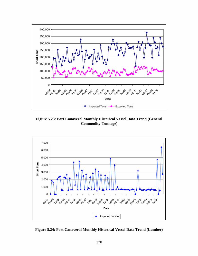
170
0
50,000
100,000
150,000
200,000
250,000
300,000
350,000
400,000
Oct-94
Feb-9
5Jun
-95Oct-9
5Fe
b-96
Jun-96
Oct-96
Feb-9
7Jun
-97Oct-9
7Fe
b-98Jun
-98Oct-9
8Fe
b-99
Jun-99
Oct-99
Feb-0
0Jun
-00Oct-0
0Fe
b-01Jun
-01
Date
Sh
ort
To
ns
Imported Tons Exported Tons
Figure 5.23: Port Canaveral Monthly Historical Vessel Data Trend (General Commodity Tonnage)
0
1,000
2,000
3,000
4,000
5,000
6,000
7,000
Oct-94Fe
b-95
Jun-95
Oct-95
Feb-9
6Jun
-96Oct-9
6Fe
b-97
Jun-97
Oct-97
Feb-9
8Jun
-98Oct-9
8Fe
b-99
Jun-99
Oct-99
Feb-0
0Jun
-00Oct-0
0Fe
b-01
Jun-01
Date
Sh
ort
To
ns
Imported Lumber
Figure 5.24: Port Canaveral Monthly Historical Vessel Data Trend (Lumber)

171
The ARIMA model was executed to produce a short term five year forecast of the
vessel freight data at Port Canaveral. The fields selected were those used as input to the
ANN truck trip generation model. The data is produced for monthly totals just as the
historical data was provided. Then, the current daily data (provided by the port authority
as individual vessel records) is ana lyzed to determine a daily distribution for each of the
forecasted fields.
Current complete months of data were available for November 2001 through
March 2002. The daily distribution from each of these months was applied to the
corresponding forecasted months to obtain daily forecast values that were used as input to
the ANN model. Table 5.20 displays the monthly forecasted vessel freight data. Table
5.21 through Table 5.23 are the results from applying the daily distribution for one week
(Monday to Friday) from each month of the forecasted data. This was the data that is
used by the ANN model to generate the daily truck volumes corresponding to each of
these weekdays. Forecasted lumber tonnage was converted to a Board Feet (BDFT)
estimate based on a conversion factor from the daily distribution of the current lumber
measured in BDFT. This was necessary in order to input the correct independent variable
for lumber by unit type (BDFT) into the ANN model. Figure 5.25 and Figure 5.26
display the trends for the vessel data including the forecasted data. Figure 5.27 shows the
percent change of the forecasted freight variables. All commodities are predicted to
increase for Port Canaveral. This is consistent with the future growth plans of the port
authority that has been confirmed during several discussions with port authority
personnel.

172
Table 5.24 through Table 5.26 are the forecasted daily truck volume results of the
ANN model. Figure 5.28 shows the trend of truck volumes from current year 2002
through forecasted year 2006. It also captures the seasonal variations at the port Figure
5.29 graphically displays the change in trucks between the current truck volumes
collected and the forecasted ANN data.
Imported Exported Imported ExportedTonnage Lumber* Tonnage Tonnage Lumber* Tonnage
Jan-02 305360 4094 102670 Jul-04 360670 4885 108420Feb-02 306480 3657 102070 Aug-04 362460 4918 108600Mar-02 312970 4096 102860 Sep-04 364260 4951 108790Apr-02 311740 3987 103290 Oct-04 366050 4984 108970May-02 313080 3947 103850 Nov-04 367840 5018 109150Jun-02 316840 4122 104130 Dec-04 369630 5051 109330Jul-02 317540 4059 104340 Jan-05 371420 5084 109510Aug-02 318990 4110 104320 Feb-05 373220 5117 109700Sep-02 321600 4176 104320 Mar-05 375010 5151 109880Oct-02 323050 4169 104500 Apr-05 376800 5184 110060Nov-02 324630 4223 104680 May-05 378600 5217 110240Dec-02 326740 4257 104930 Jun-05 380390 5250 110420Jan-03 328440 4279 105160 Jul-05 382170 5284 110610Feb-03 330120 4323 105380 Aug-05 383970 5317 110790Mar-03 332030 4352 105550 Sep-05 385760 5350 110970Apr-03 333810 4384 105700 Oct-05 387560 5383 111150May-03 335540 4421 105870 Nov-05 389350 5417 111330Jun-03 337380 4451 106040 Dec-05 391140 5450 111520Jul-03 339180 4485 106220 Jan-06 392930 5483 111700Aug-03 340950 4519 106410 Feb-06 394720 5516 111880Sep-03 342750 4552 106610 Mar-06 396510 5550 112060Oct-03 344550 4585 106790 Apr-06 398310 5583 112240Nov-03 346330 4619 106970 May-06 400100 5616 112430Dec-03 348120 4652 107150 Jun-06 401900 5649 112610Jan-04 349920 4685 107330 Jul-06 403690 5683 112790Feb-04 351710 4718 107510 Aug-06 405470 5716 112970Mar-04 353500 4751 107690 Sep-06 407270 5749 113160Apr-04 355300 4785 107870 Oct-06 409060 5782 113340May-04 357080 4818 108060 Nov-06 410850 5816 113520Jun-04 358880 4851 108240 Dec-06 412650 5849 113700* measured in short tons
Month/Year
Month/Year
Table 5.20: Port Canaveral Monthly Forecasted Vessel Data

173
Imported Exported Imported ExportedMonth/Year Day
Lumber (BDFT)
Tonnage (Tons)
Tonnage (Tons)
Month/Year Day
Lumber (BDFT)
Tonnage (Tons)
Tonnage (Tons)
Jan-02 Monday 418629 8287.488 976.4178 Jan-03 Monday 437598.1 8938.183 1000.098Tuesday 418629 8287.488 976.4178 Tuesday 437598.1 8938.183 1000.098Wednesday 418629 7182.565 3254.726 Wednesday 437598.1 7732.053 3333.661Thursday 418629 8991.309 3261.368 Thursday 437598.1 9706.471 3340.465Friday 418629 9278.892 3646.622 Friday 437598.1 10020.4 3735.061
Feb-02 Monday 215929 11435.34 1365.306 Feb-03 Monday 255269.3 12295.3 1409.582Tuesday 215929 12451.85 1365.306 Tuesday 255269.3 13396.23 1409.582Wednesday 215929 13417.86 1372.934 Wednesday 255269.3 14442.48 1417.456Thursday 215929 13416.45 6681.611 Thursday 255269.3 14440.97 6898.287Friday 215929 14342.45 6681.611 Friday 255269.3 15443.89 6898.287
Mar-02 Monday 193298 12690.65 5088.118 Mar-03 Monday 205403.6 13479.66 5221.182Tuesday 193298 12689.05 5088.118 Tuesday 205403.6 13478.02 5221.182Wednesday 441720 12689.05 5088.118 Wednesday 469383.4 13478.02 5221.182Thursday 441720 11054.52 6412.867 Thursday 469383.4 11714.08 6580.576Friday 441720 9998.498 6196.581 Friday 469383.4 10574.45 6358.634
Nov-02 Monday 568720.5 8600.245 5642.926 Nov-03 Monday 621924.4 9186.526 5766.371Tuesday 354724 11085.19 5642.926 Tuesday 387908.5 11854.27 5766.371Wednesday 354724 11161.3 5916.371 Wednesday 387908.5 11934.65 6045.799Thursday 354724 11161.3 5642.926 Thursday 387908.5 11934.65 5766.371Friday 354724 8541.264 5642.926 Friday 387908.5 9129.544 5766.371
Dec-02 Monday 240247.9 10357.87 4271.787 Dec-03 Monday 262493.4 11072.01 4362.165Tuesday 40688.39 10357.87 4271.787 Tuesday 44455.88 11072.01 4362.165Wednesday 40688.39 9933.057 4932.897 Wednesday 44455.88 10624.69 5037.262Thursday 40688.39 7191.527 4932.897 Thursday 44455.88 7682.568 5037.262Friday 40688.39 8567.35 4941.372 Friday 44455.88 9159.058 5045.917
Table 5.21: Port Canaveral Daily Forecasted Vessel Data (Year 2002-2003)

174
Imported Exported Imported ExportedMonth/Year Day
Lumber (BDFT)
Tonnage (Tons)
Tonnage (Tons)
Month/Year Day
Lumber (BDFT)
Tonnage (Tons)
Tonnage (Tons)
Jan-04 Monday 479084.7 9503.289 1020.736 Jan-05 Monday 519886.1 10069.1 1041.468Tuesday 479084.7 9503.289 1020.736 Tuesday 519886.1 10069.1 1041.468Wednesday 479084.7 8232.44 3402.452 Wednesday 519886.1 8733.342 3471.56Thursday 479084.7 10312.8 3409.396 Thursday 519886.1 10919.96 3478.645Friday 479084.7 10643.57 3812.135 Friday 519886.1 11267.63 3889.564
Feb-04 Monday 278618.4 13071.85 1438.073 Feb-05 Monday 302180.1 13844.44 1467.367Tuesday 278618.4 14252.27 1438.073 Tuesday 302180.1 15104.36 1467.367Wednesday 278618.4 15374.1 1446.107 Wednesday 302180.1 16301.76 1475.564Thursday 278618.4 15372.51 7037.719 Thursday 302180.1 16300.09 7181.079Friday 278618.4 16447.87 7037.719 Friday 302180.1 17447.9 7181.079
Mar-04 Monday 224244 14358.16 5327.04 Mar-05 Monday 243079.7 15238.11 5435.372Tuesday 224244 14356.42 5327.04 Tuesday 243079.7 15236.29 5435.372Wednesday 512437 14356.42 5327.04 Wednesday 555479.9 15236.29 5435.372Thursday 512437 12465.74 6713.996 Thursday 555479.9 13218.94 6850.533Friday 512437 11244.22 6487.554 Friday 555479.9 11915.6 6619.486
Nov-04 Monday 675653.5 9768.85 5883.887 Nov-05 Monday 729382.6 10351.09 6001.403Tuesday 421420.6 12619.52 5883.887 Tuesday 454932.7 13384.56 6001.403Wednesday 421420.6 12704.04 6169.01 Wednesday 454932.7 13473.23 6292.22Thursday 421420.6 12704.04 5883.887 Thursday 454932.7 13473.23 6001.403Friday 421420.6 9714.464 5883.887 Friday 454932.7 10299.26 6001.403
Dec-04 Monday 285021.1 11788.16 4450.914 Dec-05 Monday 307543.1 12504.55 4540.071Tuesday 48271.17 11788.16 4450.914 Tuesday 52085.5 12504.55 4540.071Wednesday 48271.17 11317.87 5139.746 Wednesday 52085.5 12011.31 5242.701Thursday 48271.17 8175.286 5139.746 Thursday 52085.5 8668.135 5242.701Friday 48271.17 9752.375 5148.578 Friday 52085.5 10345.89 5251.709
Table 5.22: Port Canaveral Daily Forecasted Vessel Data (Year 2004-2005)
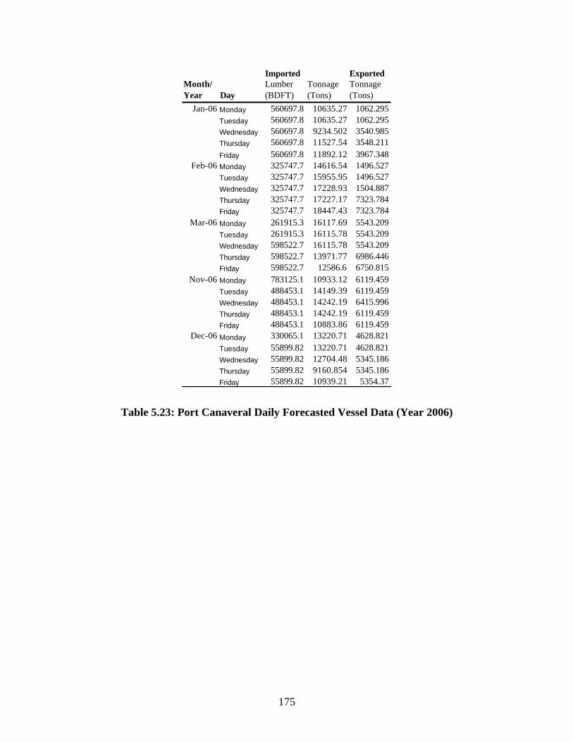
175
Imported ExportedMonth/Year Day
Lumber (BDFT)
Tonnage (Tons)
Tonnage (Tons)
Jan-06 Monday 560697.8 10635.27 1062.295Tuesday 560697.8 10635.27 1062.295Wednesday 560697.8 9234.502 3540.985Thursday 560697.8 11527.54 3548.211Friday 560697.8 11892.12 3967.348
Feb-06 Monday 325747.7 14616.54 1496.527Tuesday 325747.7 15955.95 1496.527Wednesday 325747.7 17228.93 1504.887Thursday 325747.7 17227.17 7323.784Friday 325747.7 18447.43 7323.784
Mar-06 Monday 261915.3 16117.69 5543.209Tuesday 261915.3 16115.78 5543.209Wednesday 598522.7 16115.78 5543.209Thursday 598522.7 13971.77 6986.446Friday 598522.7 12586.6 6750.815
Nov-06 Monday 783125.1 10933.12 6119.459Tuesday 488453.1 14149.39 6119.459Wednesday 488453.1 14242.19 6415.996Thursday 488453.1 14242.19 6119.459Friday 488453.1 10883.86 6119.459
Dec-06 Monday 330065.1 13220.71 4628.821Tuesday 55899.82 13220.71 4628.821Wednesday 55899.82 12704.48 5345.186Thursday 55899.82 9160.854 5345.186Friday 55899.82 10939.21 5354.37
Table 5.23: Port Canaveral Daily Forecasted Vessel Data (Year 2006)

176
Month/Year Day Inbound Outbound
Month/Year Day Inbound Outbound
Jan-02 Monday 420 459 Jan-03 Monday 439 480Jan-02 Tuesday 420 459 Jan-03 Tuesday 439 480Jan-02 Wednesday 525 394 Jan-03 Wednesday546 413Jan-02 Thursday 550 420 Jan-03 Thursday 573 441Jan-02 Friday 574 436 Jan-03 Friday 598 457Feb-02 Monday 379 312 Feb-03 Monday 413 342Feb-02 Tuesday 393 326 Feb-03 Tuesday 428 358Feb-02 Wednesday 406 340 Feb-03 Wednesday443 373Feb-02 Thursday 686 499 Feb-03 Thursday 731 536Feb-02 Friday 699 512 Feb-03 Friday 745 551Mar-02 Monday 581 431 Mar-03 Monday 605 452Mar-02 Tuesday 581 431 Mar-03 Tuesday 605 452Mar-02 Wednesday 708 537 Mar-03 Wednesday739 564Mar-02 Thursday 755 553 Mar-03 Thursday 787 579Mar-02 Friday 730 532 Mar-03 Friday 760 556Nov-02 Monday 746 549 Nov-03 Monday 788 584Nov-02 Tuesday 671 494 Nov-03 Tuesday 705 522Nov-02 Wednesday 686 503 Nov-03 Wednesday720 532Nov-02 Thursday 672 495 Nov-03 Thursday 706 523Nov-02 Friday 636 458 Nov-03 Friday 668 484Dec-02 Monday 530 394 Dec-03 Monday 556 416Dec-02 Tuesday 428 309 Dec-03 Tuesday 445 323Dec-02 Wednesday 457 322 Dec-03 Wednesday474 337Dec-02 Thursday 420 283 Dec-03 Thursday 434 295Dec-02 Friday 439 303 Dec-03 Friday 455 316
Table 5.24: Port Canaveral Daily Forecasted Truck Volumes (Year 2002-2003)

177
Month/Year Day Inbound Outbound
Month/Year Day Inbound Outbound
Jan-04 Monday 469 515 Jan-05 Monday 499 541Jan-04 Tuesday 469 515 Jan-05 Tuesday 499 541Jan-04 Wednesday 578 439 Jan-05 Wednesday 609 466Jan-04 Thursday 606 469 Jan-05 Thursday 639 497Jan-04 Friday 632 486 Jan-05 Friday 665 514Feb-04 Monday 437 364 Feb-05 Monday 461 386Feb-04 Tuesday 453 381 Feb-05 Tuesday 478 404Feb-04 Wednesday 469 397 Feb-05 Wednesday 495 421Feb-04 Thursday 763 564 Feb-05 Thursday 795 591Feb-04 Friday 778 579 Feb-05 Friday 811 607Mar-04 Monday 632 475 Mar-05 Monday 659 499Mar-04 Tuesday 632 475 Mar-05 Tuesday 659 499Mar-04 Wednesday 779 597 Mar-05 Wednesday 818 631Mar-04 Thursday 826 612 Mar-05 Thursday 866 645Mar-04 Friday 798 588 Mar-05 Friday 836 619Nov-04 Monday 829 618 Nov-05 Monday 871 652Nov-04 Tuesday 738 551 Nov-05 Tuesday 772 579Nov-04 Wednesday 754 561 Nov-05 Wednesday 788 589Nov-04 Thursday 739 552 Nov-05 Thursday 773 581Nov-04 Friday 699 510 Nov-05 Friday 730 536Dec-04 Monday 582 439 Dec-05 Monday 608 461Dec-04 Tuesday 461 338 Dec-05 Tuesday 477 352Dec-04 Wednesday 491 352 Dec-05 Wednesday 508 366Dec-04 Thursday 448 307 Dec-05 Thursday 462 318Dec-04 Friday 470 330 Dec-05 Friday 486 343
Table 5.25: Port Canaveral Daily Forecasted Truck Volumes (Year 2004-2005)
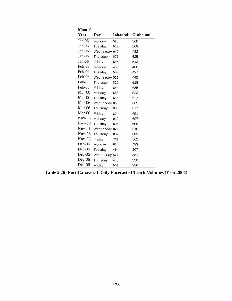
178
Month/Year Day Inbound OutboundJan-06 Monday 528 568Jan-06 Tuesday 528 568Jan-06 Wednesday 640 492Jan-06 Thursday 671 525Jan-06 Friday 698 543Feb-06 Monday 485 408Feb-06 Tuesday 503 427Feb-06 Wednesday 521 445Feb-06 Thursday 827 618Feb-06 Friday 844 635Mar-06 Monday 686 523Mar-06 Tuesday 686 523Mar-06 Wednesday 858 665Mar-06 Thursday 905 677Mar-06 Friday 874 651Nov-06 Monday 912 687Nov-06 Tuesday 805 608Nov-06 Wednesday 822 618Nov-06 Thursday 807 609Nov-06 Friday 761 562Dec-06 Monday 634 483Dec-06 Tuesday 494 367Dec-06 Wednesday 524 381Dec-06 Thursday 476 330Dec-06 Friday 501 356
Table 5.26: Port Canaveral Daily Forecasted Truck Volumes (Year 2006)

179
0
50,000
100,000
150,000
200,000
250,000
300,000
350,000
400,000
450,000
Oct-94
Oct-95
Oct-96
Oct-97
Oct-98
Oct-99
Oct-00
Oct-01
Oct-02
Oct-03
Oct-04
Oct-05
Oct-06
Date
Sho
rt T
ons
Imported Tons Exported Tons
Figure 5.25: Port Canaveral Vessel Data Trend (General Commodity Tonnage)
0
1,000
2,000
3,000
4,000
5,000
6,000
7,000
Oct-94
Oct-95
Oct-96
Oct-97
Oct-98
Oct-99
Oct-00
Oct-01
Oct-02
Oct-03
Oct-04
Oct-05
Oct-06
Date
Sho
rt T
ons
Imported Lumber
Figure 5.26: Port Canaveral Monthly Vessel Data Trend (Lumber)

180
27.24%
39.18%
8.55%
0%
5%
10%
15%
20%
25%
30%
35%
40%
45%
Imported Tons Imported Lumber* Exported Tons
% C
han
ge
Figure 5.27: Port Canaveral Forecasted Change in Freight Movements (2002-2006)

181
0
100
200
300
400
500
600
700
800
900
1000
2001 2002 2003 2004 2005 2006
Year2
Po
rt C
anav
eral
Dai
ly T
ruck
Vo
lum
e1
Inbound
Outbound
1excludes weekends2annual counts using one week from each month of the year (84 data points)
Figure 5.28: Port Canaveral Forecasted Truck Movements (2002-2006)

182
0
100
200
300
400
500
600
700
800
Inbound Outbound
Ave
rage
Dai
ly T
ruck
Vol
ume
20022006
Figure 5.29: Port Canaveral Change in Forecasted Truck Movements (2002-2006)
5.4.4 Port Canaveral Network Forecasting
Once the forecasted daily truck volumes generated by Port Canaveral vessel
freight activity were determined, they must be converted to peak hourly traffic volumes.
In order to execute the VISSIM network model, it requires hour ly traffic volumes that
include all vehicle types. The methodology developed for the Tampa model was applied
to Port Canaveral. This procedure is detailed previously in section 4.4 for the Port of
Tampa. A selection of data from the ANN forecast results were used to compute the
necessary hourly traffic volumes. These results are shown in Table 5.27.

183
Inbound Outbound
DateDay of the Week
Peak Hour Traffic
Peak Hour Trucks
Peak Hour Traffic
Peak Hour Trucks
Jan-06 Monday 345 35 797 80Jan-06 Tuesday 345 35 797 80Jan-06 Wednesday 418 42 690 69Jan-06 Thursday 438 44 737 74Jan-06 Friday 456 46 762 76
Table 5.27: Port Canaveral Freight Terminal Hourly Traffic Volumes for Year 2006
Also, to estimate the change in traffic volumes on the network, the growth factor
was calculated from the growth in truck volumes using the same methodology from the
Tampa analysis. The growth factor was calcula ted from both inbound and outbound
truck volumes for two months and an average percent of growth determined. The percent
growth was found to be 38.13%.
Once the peak hourly traffic volumes generated by Port Canaveral’s freight vessel
activity are estimated and the growth factor applied to the network volumes, an O-D
matrix for each of the 5 days of forecasted daily truck data was concluded. According to
the ANN Port Canaveral truck trip generation modeling results from the January 2006
data selection for trucks destined to Port Canaveral generated by the port’s vessel freight
activity, 15.4% use SR 528 (eastbound), 12.4% use I-95 traveling northbound (coming
from areas south of SR 528) and 12.4% use I-95 traveling southbound (coming from
areas north of SR 528). For trucks originating from Port Canaveral, 19.3% use SR 528
(westbound), 19.3% use I-95 traveling northbound (going to areas north of SR 528) and
8.0% use I-95 traveling southbound (going to areas south of SR 528).
The network model has also captured port generated local truck trips. 12.8% of
the truck traffic generated by the port’s freight activity travel to Industry Road and 30.9%

184
of the trucks destined to the port are coming from Industry Road. This Industry Road
truck traffic is attributed to the large Rinker cement facility. Also, 12.8% of the trucks
were local trips to US1 and 9.3% of the truck trips to the port were from US1. This truck
traffic is attributed to the rail terminal located just northwest of SR 528. The results of
the forecasting on the network are shown in Table 5.28.
LocationSR 528 (Link # 7)*
SR 528 (Link # 8)*
SR 528 (Link # 15)*
Date Weekday Direction VISSIM VISSIM VISSIMJan-06 Monday Inbound 43 27 14
Outbound 71 56 27Jan-06 Tuesday Inbound 43 27 14
Outbound 71 56 27Jan-06 Wednesday Inbound 43 28 15
Outbound 72 55 28Jan-06 Thursday Inbound 43 27 14
Outbound 72 55 29Jan-06 Friday Inbound 45 28 14
Outbound 73 55 28* denotes a master link
Table 5.28: Port Canaveral Network Peak Hour Truck Volumes (Year 2006)
185
6. CONCLUSIONS AND RECOMMENDATIONS
A microscopic simulation computer modeling approach was successfully utilized
in the development of a methodology for modeling Florida seaport generated heavy
trucks on a road network adjacent to the seaport. Two micro simulation-modeling
packages were evaluated in the methodology development using data from the Port of
Tampa. Both CORSIM and VISSIM produced acceptable results when compared to
truck volumes collected from the field at the port and selected locations on the defined
road network. A short-term forecast of truck volumes was performed to examine the
increase of trucks on the road network due to an increase in seaport generated truck
volumes. The transferability of this methodology was successfully tested for Port
Canaveral.
Once the appropriate road network was defined, the computer models were
calibrated with FDOT and field collected traffic volumes. These traffic volumes
consisted of heavy trucks only and total vehicular traffic (all vehicle types). After the
models were calibrated, a validation was performed and statistically verified at the 95%
confidence level. The validation was conducted with actual field collected truck volumes
not used in the calibration.
The results of the network modeling and analysis indicated that an average of 720
heavy trucks generated by the Port of Tampa’s freight activity travel on the defined
network during the peak hour (5-6 PM). From this total truck traffic, 55% of these trucks
travel between the port’s freight terminals and the connecting interstate highways (I-4, I-
275, I-75). Interstate 4 was found to serve the highest percent of trucks generated by the

186
port. For trucks traveling to the port, 22% of the total trucks are estimated to come from
I-4 and 38% leaving the port are destined to I-4. Also, due to the high volumes of
phosphate products handled at the Port of Tampa, Causeway Boulevard serves an
estimated 250 trucks during the peak hour generated by the port’s freight activity.
The comparison between CORSIM and VISSIM results indicated that both
computer simulation packages produce similar results. Overall however, VISSIM is
more user friendly, takes less time to develop a model, and the animation is better
including 3-D animation features. CORSIM does provide an overall network evaluation
value whereas VISSIM does not. But, this can be obtained from the VISSIM results with
a minor computation step. CORSIM also currently has a more user friendly signal
coding module but VISSIM developers were working on improving this. VISSIM was
concluded to be a better computer package for application to the network modeling and
selected to conduct the short term forecasting for the Port of Tampa and also the
transferability testing on Port Canaveral.
To conduct a short-term forecast of the truck traffic estimated on the identified
routes used by trucks generated by the Port of Tampa in year 2005, a truck trip generation
model previously developed for the Port of Tampa was executed. The results from this
model were used to determine the input for the developed Port of Tampa road network
model. A growth factor of 6% was calculated for the defined road network based on
estimated growth at the port.
From the analysis of results for the short term forecast on the Port of Tampa road
network, the overall heavy truck traffic on the defined network generated by the port was
estimated to increase by 4.5%. This low increase is attributed to the previous forecasted

187
results of the minute increase in freight activity for the port. Most of the truck volumes
related to the interstate highways show only minor incremental increases during the peak
hour. Interstate 75 displayed the largest increase from 6% to 14% of the total trucks
generated by the port.
A sensitivity analysis was conducted on the defined network to test the developed
methodology for intelligent transportation systems (ITS) applications such as Advanced
Traveler Information Systems (ATIS) or incident management. Four scenarios were
conducted including a base scenario. Average travel time and delay for the entire
network were selected as the measures of effectiveness (MOEs).
The existing conditions (base scenario) produced an average travel time for the
network of 329 sec/veh and an average delay of 113 sec/veh. Scenario 2, which was
adding one lane for each direction to the access roads north of Hookers Point (22nd and
21st Streets), decreased the average network travel time by 8% and the average delay by
12%. Scenario 3 evaluated the network if the trucks were prohibited from using 22nd and
21st Streets. Compared to the base scenario, the average travel time increased by 6% and
the average delay increased by 5% for the entire network. However, the travel time and
delay have decreased by approximately 50% for the routes between Hooker’s Point and
the Interstates to the north (I-4 and I-275) using 22nd and 21st Streets. Scenario 4
examines the network with an incident occurrence on 22nd Street where one lane is closed
to through traffic. Compared to the base scenario, the average travel time increased by
17% and the average delay increased by 16% for the entire network.
After the developed methodology was successfully tested and implemented for
short term forecasting with the Port of Tampa, the methodology was applied to Port

188
Canaveral. Port Canaveral’s network was smaller than Tampa and the port generates
much lower traffic volumes overall. Port Canaveral also has lower freight activity than
Tampa.
The Port of Tampa has a number of main truck routes directly feeding into the
port whereas Port Canaveral has only SR 528. There is another route to the south (SR
A1A to SR 520), but it is a low speed arterial that is not suitable for heavy truck traffic
however could be utilized as an alternate route if necessary during a emergency situation.
This was included in the Port Canaveral network definition for ITS applications.
The Port Canaveral road network was defined and modeled using VISSIM. The
calibrated model was validated at the 95% confidence level using field data collected on
the selected master links. The master links were all located on SR 528 however, they
also capture the truck traffic on Interstate 95 generated by the port’s freight activity. Of
the total truck volumes generated by the port during the peak hour, on the average, 25%
of the trucks generated by the port use I-95 and 18% use SR 528 for travel outside the
defined network. Due to the local destinations on the network (US 1 rail terminal,
Industry Road Rinker Cement facility), there are also a significant percent of local trips
made in the area captured by the defined network as well. On the average, 11% of the
total truck trips travel between US 1 (rail terminal) and the port and 22% of the total
truck trips travel between Industry Road (Rinker Cement Distribution Facility) and the
port.
In order to conduct the short term forecasting of the port generated heavy truck
traffic on the network, a truck trip generation is required. This model was developed for
Port Canaveral with the same methodology as in Phase II of this project (11). The model

189
was successfully validated at the 95% confidence level with 45 days of field data
collected at Port Canaveral’s freight terminals. From historical vessel freight data, a
short term (5-year) forecast was done using a time series modeling approach to obtain an
estimate of the daily heavy trucks that the port would generate in years 2002 through
2006. The truck trip generation model has shown to be robust because it successfully
captured seasonal truck traffic trends at the port as well.
Port Canaveral is projected to have a significant growth of its vessel freight
activity. Using the results of year 2006, the truck volumes were used to determine the
input for the Port Canaveral road network model. The growth factor based on the
estimated future freight activity is significant at 38%. The distribution of trucks on the
network however stays virtually unchanged. This is attributed to the simplicity of the
network compared to Tampa. There is only one main access highway to the port that
services heavy trucks (SR 528) and only two routes (SR 528 and I-95) are currently used
for interstate and intrastate travel by the trucks generated from Port Canaveral’s freight
activity.
The methodology developed for modeling truck traffic generated by a Florida
seaport’s freight activity has been successfully tested for the Port of Tampa and applied
in practice to Port Canaveral. Furthermore, the developed road network models utilize
previously developed truck trip generation models for these two ports to determine short-
term forecasts of truck volumes at the port. These forecasted truck volumes were used to
determine the input data for the desired forecast year and the network was successfully
modeled for that year. Due to the successful transferability testing, this methodology can
be applied to any other Florida seaport.

190
The ANN trip generation model output is useful for determining the number of
trucks expected to be generated by a facility with freight activity. The developed
network methodology herein has proven the usefulness of this data. This model data can
be utilized as input to other models such as the Florida Statewide Freight Model.
Similarly, the developed network models can be utilized by local transportation and
planning agencies to investigate the impacts of heavy trucks in areas with freight activity.
These network models provide the agencies with a microscopic modeling approach for
local traffic situations.
The developed road network models for Tampa and Cape Canaveral have
application to any traffic study that would include the seaport in the network. The
network models can be utilized to test the occurrence of new security measures for access
to the port’s freight terminal facilities. The network can be tested for alternate route
choice. Intelligent Transportation System (ITS) applications can be tested on the network
before deployment as well.
Scenarios based on estimated future port growth or changes to seasonal freight
movements can also be tested to determine what impact these changes could have on the
network in terms of travel time and delay. Local municipalities can determine if
estimated growth will impact the network and if so, can test geometric improvement
scenarios. These seaports are special generators of traffic and these models can be
utilized to determine input for other broader computer models for planning and
development purposes.

191
APPENDIX A Trip Reports

192
TRUCK PROJECT REPORT Date/Location: November 5-6, 2000 / Tampa (phase 2I)
Travelers: Anand Jujare, Ahmed Elhelw
Subject: Meeting with City of Tampa Transportation Department
Objective: Obtaining Volumes of traffic and signal timing for different nodes
and links
Outcome: Successful
Summary: A meeting was held with City of Tampa Transportation Department. A brief summery of
the project was provided to Mr. Mike Scanner (Head of traffic operations section). A
map showing nodes and links of the proposed network was also provided. Traffic
volumes at all the nodes that are west of 50th street were obtained. Hillsborough County
controls streets that are east of 50th street. Signal timing and turning movements’
volumes were also obtained for the above mentioned nodes. Signal timing was obtained
in two forms, namely basic and different patterns. Basic and all the different timing
patterns for each signal (actuated ones) were also obtained. A sample of these data is
shown in the attached sheet. All the data was obtained as hard copies. Another meeting
should be held with City of Tampa TD to get any available data on the links for the same
area. City of Tampa identified contact persons in Hillsborough County. Another meeting
should be held with Mr. Greg Basset in Hillsborough County to get the same type of data
for the rest of the network. People of City of Tampa were cooperative and helpful.
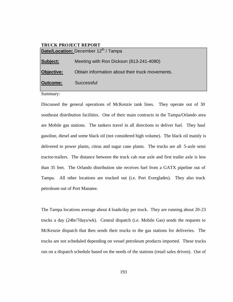
193
TRUCK PROJECT REPORT Date/Location: December 12th / Tampa
Subject: Meeting with Ron Dickson (813-241-4080)
Objective: Obtain information about their truck movements.
Outcome: Successful
Summary:
Discussed the general operations of McKenzie tank lines. They operate out of 30
southeast distribution facilities. One of their main contracts in the Tampa/Orlando area
are Mobile gas stations. The tankers travel in all directions to deliver fuel. They haul
gasoline, diesel and some black oil (not considered high volume). The black oil mainly is
delivered to power plants, citrus and sugar cane plants. The trucks are all 5-axle semi
tractor-trailers. The distance between the truck cab rear axle and first trailer axle is less
than 35 feet. The Orlando distribution site receives fuel from a GATX pipeline out of
Tampa. All other locations are trucked out (i.e. Port Everglades). They also truck
petroleum out of Port Manatee.
The Tampa locations average about 4 loads/day per truck. They are running about 20-23
trucks a day (24hr/7days/wk). Central dispatch (i.e. Mobile Gas) sends the requests to
McKenzie dispatch that then sends their trucks to the gas stations for deliveries. The
trucks are not scheduled depending on vessel petroleum products imported. These trucks
run on a dispatch schedule based on the needs of the stations (retail sales driven). Out of

194
Tampa, the trucks mainly travel 22nd st and Causeway blvd to Hwy 301 and 41. They
also use I-75 and I-275 for longer distance trips.
Ft. Lauderdale (Port Everglades) McKenzie lines use the interstates for their trips. They
are running about 35 to 40 trucks/day and also average about 4 loads/day.
The Terminal locations are:
Bucks, AL Mobile, AL Opelika, AL
Brooker, FL Ft. Lauderdale, FL Jacksonville, FL
Panama City, FL Pensacola, FL Port Manatee, FL
St. Marks, FL Taft, FL Tallahasse, FL
Tampa, FL Albany, GA Alma, GA
Bainbridge, GA Jesup, GA Milner, GA
Savannah, GA Augusta, GA Chicago, IL
Catlettsburg, KY Hahnville, LA St. Gabriel, LA
Charlotte, NC Charleston, SC Clarksville, TN
Beaumont, TX Brownsville, TX Houston, TX

195
Nodes # Description Link # Description Length Speed limit Notes State Road
1 U.S. Highway 41 / Madison Avenue 1 Node 1 to Node 2 2.62 45 mph 2 Lane highway
2 78th street / Madison Avenue 2 Node 2 to Node 3 2.69 35 mph 2 Lane highway
3 Madison Avenue / U.S. Highway 301 3 Node 3 to Node 4 0.78 50 mph 2 Lane highway SR 301
4 U.S. Highway 301 / I-75 4 Node 4 to Node 5 1.45 50 mph 6 Lane divided SR 301
5 State road 676 / U.S. Highway 301 5 Node 5 to Node 6 0.6 50 mph 6 Lane divided SR 301
6 Expressway 618 / U.S. Highway 301 6 Node 6 to Node 7 1.34 50 mph 6 Lane divided SR 301
7 State Highway 60 / U.S. Highway 301 7 Node 7 to Node 8 2.3 50 mph 6 Lane divided SR 301
8 State Highway 574 / U.S. Highway 301 8 Node 8 to Node 9 1.44 50 mph 4 Lane undivided
9 State Highway 574 / I-4 9 Node 9 to Node 10 1.48 55 mph 6 Lane divided I-4
10 22nd Street / I-4 10 Node 10 to Node 11 1.95 55 mph 4 Lane divided I-4
11 I-4 / I-275 11 Node 11 to Node 12 1.16 55 mph 4 Lane divided I-275
12 State Highway 92 / I-275 12 Node 12 to Node 13 3.85 45 mph 6 Lane divided SR 92
13 State Highway 92 / State Highway 60 13 Node 13 to Node 14 0.68 45 mph 6 Lane divided SR 92
14 State Highway 92 / State Highway 618 14 Node 14 to Node 15 3.35 65 mph 4 Lane undivided SR 618
15 State Highway 60 / Expressway 618 15 Node 15 to Node 16 5.61 65 mph 4 Lane divided SR 618
16 22nd Street / Expressway 618 16 Node 16 to Node 17 1.33 65 mph 4 Lane divided SR 618
17 State Highway 41 / Expressway 618 17 Node 17 to Node 18 2.15 65 mph 6 Lane divided SR 41
18 State road 676 / U.S. Highway 41 18 Node 18 to Node 1 1.87 55 mph 6 Lane divided SR 41
19 State Highway 41 / State Highway 60 19 Node 19 to Node 17 1.49 55 mph 6 Lane divided SR 41
20 22nd Street / State Highway 60 20 Node 21 to Node 5 1.12 45 mph 4 Lane divided SR 676
21 State road 676 / 78th street 21 Node 2 to Node 21 1.6 45 mph 2 Lane highway
22 Node 21 to Node 18 3.85 45 mph 2 Lane highway SR 676
23 Node 6 to Node 17 2.91 55 mph 6 Lane divided SR 618
24 Node 19 to Node 7 0.15 35 mph 6 Lane divided SR 60
25 Node 10 to Node 20 1.05 55 mph 4 Lane divided
26 Node 20 to Node 16 2.07 55 mph 6 Lane divided
27 Node 19 to Node 20 3.42 55 mph 6 Lane divided SR 60
28 Node 15 to Node 20 0.64 35 mph 2 Lane highway SR 60
29 Node 13 to Node 15 3.42 55 mph 6 Lane divided SR 60
30 Node 9 to Node 19 3.42 55 mph 6 Lane divided SR 41
Table A. 1: Data Gathered for the Links of Port of Tampa Road Network

Jack Klodzinski April 16, 2002/Canaveral
196
TRUCK PROJECT REPORT Date/Location: April 16, 2002 / Canaveral
Subject: vehicle classifier equipment maintenance Objective: download data, conduct routine maintenance on classifiers. Outcome: successful
Summary:
Routine maintenance of vehicle classifiers that are used to identify the number of heavy trucks entering and leaving the Port Canaveral facilities was conducted. Download of data from the classifiers was not accomplished for all locations (freight terminals and network locations). Several classifiers were repaired. One location was repaired. Another trip is required to test the viability of fiber optic sensor usage as an alternative to the tube counters for the dual lanes on SR528.
For Traffic Classifier Status, see Table 1.
To Do:
1. Test Fiber optic sensors. 2. Installation of new SR 528 locations. 3. Check geometric features from Brevard County with field observations.
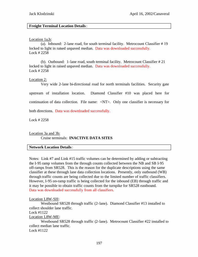
Jack Klodzinski April 16, 2002/Canaveral
197
Freight Terminal Location Details :
Location 1a,b: (a). Inbound: 2-lane road, for south terminal facility. Metrocount Classifier # 19 locked to light in raised unpaved median. Data was downloaded successfully. Lock # 2258 (b). Outbound: 1- lane road, south terminal facility. Metrocount Classifier # 21 locked to light in raised unpaved median. Data was downloaded successfully. Lock # 2258 Location 2: Very wide 2- lane bi-directional road for north terminals facilities. Security gate
upstream of installation location. Diamond Classifier #10 was placed here for
continuation of data collection. File name: <NT>. Only one classifier is necessary for
both directions. Data was downloaded successfully.
Lock # 2258
Location 3a and 3b: Cruise terminals: INACTIVE DATA SITES Network Location Details :
Notes: Link #7 and Link #15 traffic volumes can be determined by adding or subtracting the I-95 ramp volumes from the through counts collected between the NB and SB I-95 off-ramps from SR528. This is the reason for the duplicate descriptions using the same classifier at these through lane data collection locations. Presently, only outbound (WB) through traffic counts are being collected due to the limited number of traffic classifiers. However, I-95 on-ramp traffic is being collected for the inbound (EB) through traffic and it may be possible to obtain traffic counts from the turnpike for SR528 eastbound. Data was downloaded successfully from all classifiers. Location L8W-SH: Westbound SR528 through traffic (2- lane). Diamond Classifier #13 installed to collect shoulder lane traffic. Lock #1122 Location L8W-ME: Westbound SR528 through traffic (2- lane). Metrocount Classifier #22 installed to collect median lane traffic. Lock #1122

Jack Klodzinski April 16, 2002/Canaveral
198
Location L8E-SH: Eastbound SR528 through traffic (2- lane). Diamond Classifier #17 installed to collect shoulder lane traffic. File name is <L8E-SHa>. Lock #112 Location L8E-ME: Eastbound SR528 through traffic (2- lane). Diamond Classifier #15 installed to collect median lane traffic. File name is <L8E-MEa>. Lock #112 Location L1W-SH: Westbound SR528 through traffic (2-lane). Diamond Classifier #07 removed. INACTIVE DATA SITES
Lock #465
Location L1W-ME: Westbound SR528 through traffic (2- lane). Diamond Classifier #18 removed. INACTIVE DATA SITES
Lock #465 Location N1-OF: Westbound SR528 1 lane off- ramp to SR3. INACTIVE DATA SITE Location N1-ON: Westbound SR528 2 lane on-ramp from SR3. INACTIVE DATA SITE Location N4-OF: Westbound SR528 1 lane off- ramp to US1. INACTIVE DATA SITE Location N4-ON: Westbound SR528 1 lane on-ramp to US1. INACTIVE DATA SITE
Location N?-OF: Westbound SR528 1 lane off-ramp to Industry Road. INACTIVE DATA SITE
Lock #489 SR524 is a two- lane undivided major arterial (55 mph) that travels through a residential area and has signalized intersections on it. It would not be a good selected route for truck drivers because of the side street traffic and signalized intersections that could create multiple deceleration and acceleration events for the trucks. Location N6-OFa: Westbound SR528 1 lane off- ramp to I-95 Northbound. Diamond Classifier #05 installed. Battery replaced. Lock #A380

Jack Klodzinski April 16, 2002/Canaveral
199
Location N6-OFb: Westbound SR528 1 lane off-ramp to I-95 Southbound. Diamond Classifier #12 installed.
Lock #325
Location L7W-SH: Westbound SR528 through traffic (2- lane). Diamond Classifier #09 installed for shoulder lane traffic counts. (traffic counts from Location N6-OFa need to be added to these counts to obtain a true through traffic count westbound to Orlando for Link #7). Lock #A380
Location L15W-SH: Westbound SR528 through traffic (2- lane). Diamond Classifier #09 installed for shoulder lane traffic counts. (traffic counts from Location N6-OFb need to be subtracted from these counts to obtain a true through traffic count westbound to Orlando for Link #15). Lock #A380
Location L7W-ME: Westbound SR528 through traffic (2- lane). Diamond Classifier #11 installed for shoulder lane traffic counts. (traffic counts from Location N6-OFa need to be added to these counts to obtain a true through traffic count westbound to Orlando for Link #7). Lock #A380
Location L15W-ME: Westbound SR528 through traffic (2- lane). Diamond Classifier #11 installed for shoulder lane traffic counts. (traffic counts from Location N6-OFb need to be subtracted from these counts to obtain a true through traffic count westbound to Orlando for Link #15). Lock #A380
Location N6-ONa: Eastbound SR528 1 lane on-ramp from I-95 Northbound. Metrocount Classifier #24 installed. Tube B was split and not collecting data. Tube was replaced. Lock #1126
Location N6-ONb: Eastbound SR528 1 lane on-ramp from I-95 Southbound. Metrocount Classifier #23 installed. Lock #1126
Location L7E-SH:
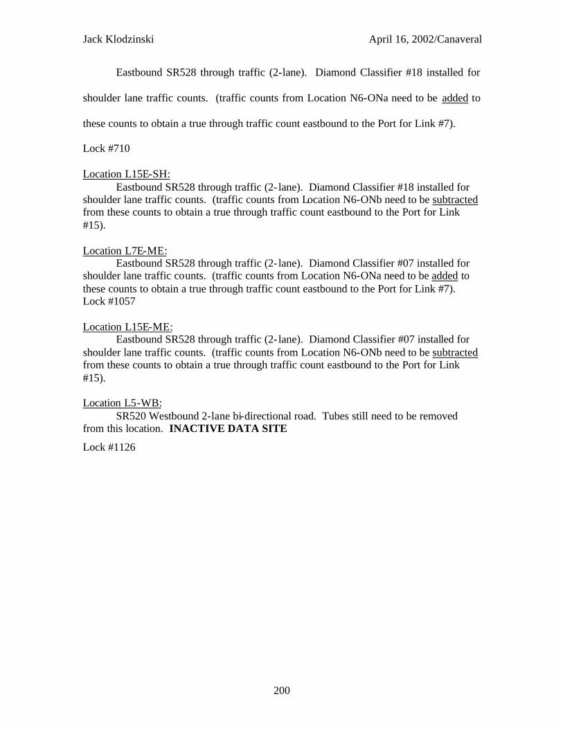
Jack Klodzinski April 16, 2002/Canaveral
200
Eastbound SR528 through traffic (2-lane). Diamond Classifier #18 installed for
shoulder lane traffic counts. (traffic counts from Location N6-ONa need to be added to
these counts to obtain a true through traffic count eastbound to the Port for Link #7).
Lock #710
Location L15E-SH: Eastbound SR528 through traffic (2- lane). Diamond Classifier #18 installed for shoulder lane traffic counts. (traffic counts from Location N6-ONb need to be subtracted from these counts to obtain a true through traffic count eastbound to the Port for Link #15). Location L7E-ME: Eastbound SR528 through traffic (2- lane). Diamond Classifier #07 installed for shoulder lane traffic counts. (traffic counts from Location N6-ONa need to be added to these counts to obtain a true through traffic count eastbound to the Port for Link #7). Lock #1057
Location L15E-ME: Eastbound SR528 through traffic (2- lane). Diamond Classifier #07 installed for shoulder lane traffic counts. (traffic counts from Location N6-ONb need to be subtracted from these counts to obtain a true through traffic count eastbound to the Port for Link #15). Location L5-WB: SR520 Westbound 2-lane bi-directional road. Tubes still need to be removed from this location. INACTIVE DATA SITE
Lock #1126
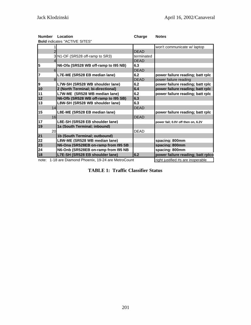
Jack Klodzinski April 16, 2002/Canaveral
201
Number Location Charge NotesBold indicates "ACTIVE SITES"
1 won't communicate w/ laptop2 DEAD3 N1-OF (SR528 off-ramp to SR3) terminated4 DEAD
5 N6-Ofa (SR528 WB off-ramp to I95 NB) 6.36 DEAD
7 L7E-ME (SR528 EB median lane) 6.2 power failure reading; batt rplc8 DEAD power failure reading
9 L7W-SH (SR528 WB shoulder lane) 6.2 power failure reading; batt rplc10 2 (North Terminal; bi-directional) 6.4 power failure reading; batt rplc11 L7W-ME (SR528 WB median lane) 6.2 power failure reading; batt rplc12 N6-Ofb (SR528 WB off-ramp to I95 SB) 6.313 L8W-SH (SR528 WB shoulder lane) 6.3
14 DEAD15 L8E-ME (SR528 EB median lane) power failure reading; batt rplc
16 DEAD17 L8E-SH (SR528 EB shoulder lane) power fail; 0.0V off then on, 6.2V19 1a (South Terminal; inbound)
20 DEAD21 1b (South Terminal; outbound)22 L8W-ME (SR528 WB median lane) spacing: 800mm23 N6-Ona (SR528EB on-ramp from I95 SB spacing: 800mm24 N6-Onb (SR528EB on-ramp from I95 NB spacing: 800mm18 L7E-SH (SR528 EB shoulder lane) 6.2 power failure reading; batt rplcon loan, no FDOT decalnote: 1-18 are Diamond Phoenix, 19-24 are MetroCount right justified #s are inoperable
TABLE 1: Traffic Classifier Status

Jack Klodzinski April 16, 2002/Canaveral
202
1
2
3a
3b
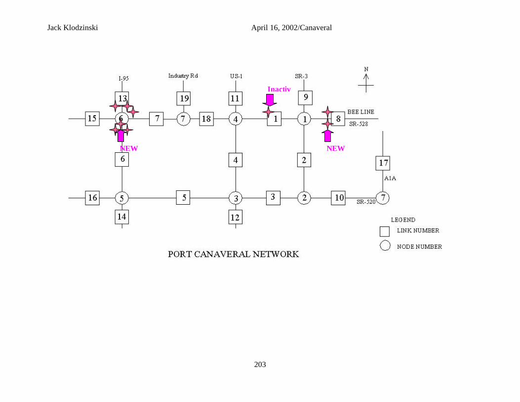
Jack Klodzinski April 16, 2002/Canaveral
203
NEW NEW
Inactiv

204
APPENDIX B Sample of Signal Timing and Intersection Data

205
Figure B. 1: Key Map Obtained from Hillsborough County

206
Figure B. 2: Sample of Turning Movements Counts

207
APPENDIX C Scheffe's Statistical Test Results for
Calibration Field Data of Master Links
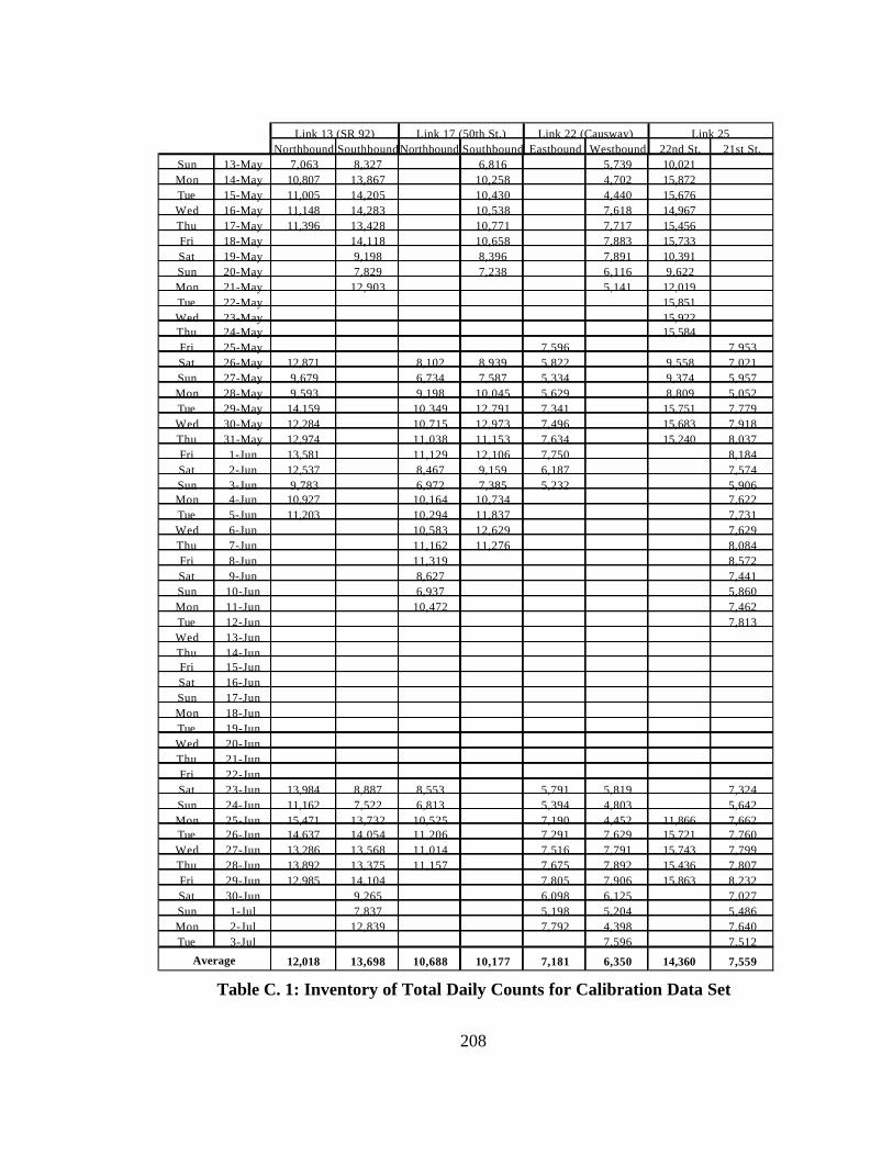
208
Table C. 1: Inventory of Total Daily Counts for Calibration Data Set
Northbound Southbound Northbound Southbound Eastbound Westbound 22nd St. 21st St.Sun 13-May 7,063 8,327 6,816 5,739 10,021Mon 14-May 10,807 13,867 10,258 4,702 15,872Tue 15-May 11,005 14,205 10,430 4,440 15,676Wed 16-May 11,148 14,283 10,538 7,618 14,967Thu 17-May 11,396 13,428 10,771 7,717 15,456Fri 18-May 14,118 10,658 7,883 15,733Sat 19-May 9,198 8,396 7,891 10,391Sun 20-May 7,829 7,238 6,116 9,622Mon 21-May 12,903 5,141 12,019Tue 22-May 15,851Wed 23-May 15,922Thu 24-May 15,584Fri 25-May 7,596 7,953Sat 26-May 12,871 8,102 8,939 5,822 9,558 7,021Sun 27-May 9,679 6,734 7,587 5,334 9,374 5,957Mon 28-May 9,593 9,198 10,045 5,629 8,809 5,052Tue 29-May 14,159 10,349 12,791 7,341 15,751 7,779Wed 30-May 12,284 10,715 12,973 7,496 15,683 7,918Thu 31-May 12,974 11,038 11,153 7,634 15,240 8,037Fri 1-Jun 13,581 11,129 12,106 7,750 8,184Sat 2-Jun 12,537 8,467 9,159 6,187 7,574Sun 3-Jun 9,783 6,972 7,385 5,232 5,906Mon 4-Jun 10,927 10,164 10,734 7,622Tue 5-Jun 11,203 10,294 11,837 7,731Wed 6-Jun 10,583 12,629 7,629Thu 7-Jun 11,162 11,276 8,084Fri 8-Jun 11,319 8,572Sat 9-Jun 8,627 7,441Sun 10-Jun 6,937 5,860Mon 11-Jun 10,472 7,462Tue 12-Jun 7,813Wed 13-JunThu 14-JunFri 15-JunSat 16-JunSun 17-JunMon 18-JunTue 19-JunWed 20-JunThu 21-JunFri 22-JunSat 23-Jun 13,984 8,887 8,553 5,791 5,819 7,324Sun 24-Jun 11,162 7,522 6,813 5,394 4,803 5,642Mon 25-Jun 15,471 13,732 10,525 7,190 4,452 11,866 7,662Tue 26-Jun 14,637 14,054 11,206 7,291 7,629 15,721 7,760Wed 27-Jun 13,286 13,568 11,014 7,516 7,791 15,743 7,799Thu 28-Jun 13,892 13,375 11,157 7,675 7,892 15,436 7,807Fri 29-Jun 12,985 14,104 7,805 7,906 15,863 8,232Sat 30-Jun 9,265 6,098 6,125 7,027Sun 1-Jul 7,837 5,198 5,204 5,486Mon 2-Jul 12,839 7,792 4,398 7,640Tue 3-Jul 7,596 7,512
12,018 13,698 10,688 10,177 7,181 6,350 14,360 7,559Average
Link 13 (SR 92) Link 17 (50th St.) Link 22 (Causway) Link 25
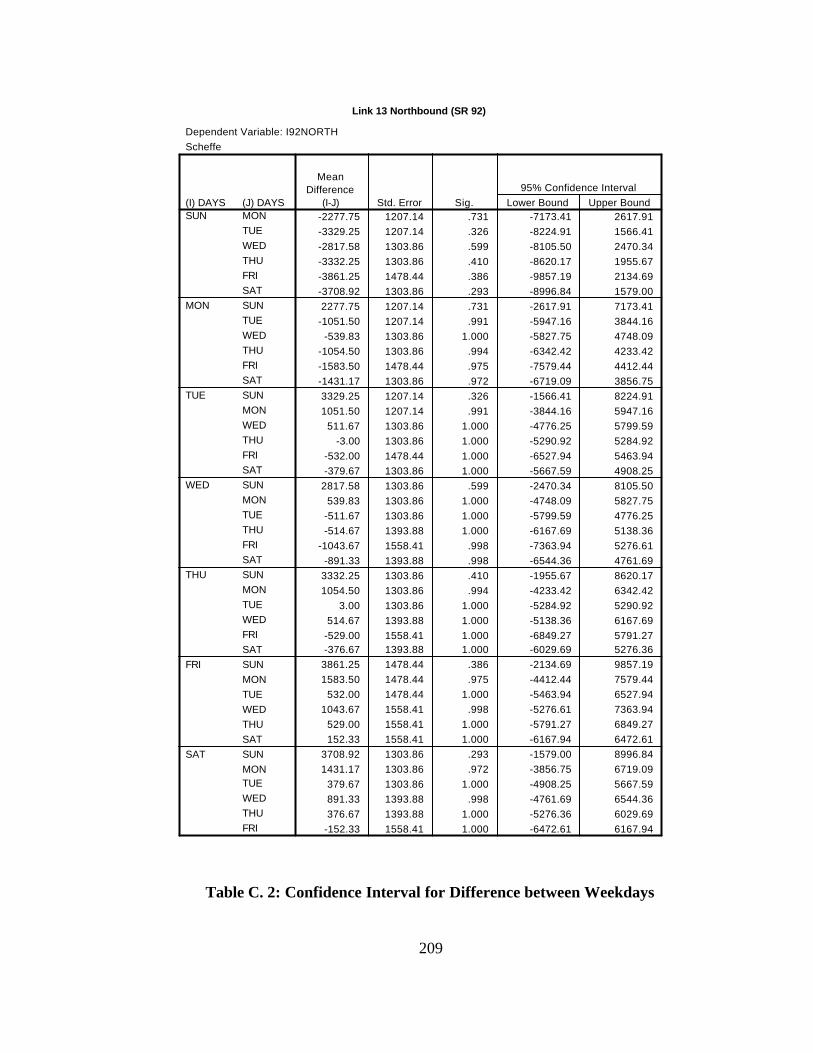
209
Link 13 Northbound (SR 92)
Dependent Variable: I92NORTHScheffe
-2277.75 1207.14 .731 -7173.41 2617.91-3329.25 1207.14 .326 -8224.91 1566.41-2817.58 1303.86 .599 -8105.50 2470.34-3332.25 1303.86 .410 -8620.17 1955.67-3861.25 1478.44 .386 -9857.19 2134.69-3708.92 1303.86 .293 -8996.84 1579.002277.75 1207.14 .731 -2617.91 7173.41
-1051.50 1207.14 .991 -5947.16 3844.16-539.83 1303.86 1.000 -5827.75 4748.09
-1054.50 1303.86 .994 -6342.42 4233.42-1583.50 1478.44 .975 -7579.44 4412.44-1431.17 1303.86 .972 -6719.09 3856.753329.25 1207.14 .326 -1566.41 8224.911051.50 1207.14 .991 -3844.16 5947.16
511.67 1303.86 1.000 -4776.25 5799.59-3.00 1303.86 1.000 -5290.92 5284.92
-532.00 1478.44 1.000 -6527.94 5463.94-379.67 1303.86 1.000 -5667.59 4908.25
2817.58 1303.86 .599 -2470.34 8105.50539.83 1303.86 1.000 -4748.09 5827.75
-511.67 1303.86 1.000 -5799.59 4776.25-514.67 1393.88 1.000 -6167.69 5138.36
-1043.67 1558.41 .998 -7363.94 5276.61-891.33 1393.88 .998 -6544.36 4761.69
3332.25 1303.86 .410 -1955.67 8620.171054.50 1303.86 .994 -4233.42 6342.42
3.00 1303.86 1.000 -5284.92 5290.92514.67 1393.88 1.000 -5138.36 6167.69
-529.00 1558.41 1.000 -6849.27 5791.27-376.67 1393.88 1.000 -6029.69 5276.36
3861.25 1478.44 .386 -2134.69 9857.191583.50 1478.44 .975 -4412.44 7579.44
532.00 1478.44 1.000 -5463.94 6527.941043.67 1558.41 .998 -5276.61 7363.94
529.00 1558.41 1.000 -5791.27 6849.27152.33 1558.41 1.000 -6167.94 6472.61
3708.92 1303.86 .293 -1579.00 8996.841431.17 1303.86 .972 -3856.75 6719.09
379.67 1303.86 1.000 -4908.25 5667.59891.33 1393.88 .998 -4761.69 6544.36376.67 1393.88 1.000 -5276.36 6029.69
-152.33 1558.41 1.000 -6472.61 6167.94
(J) DAYSMONTUEWEDTHUFRISATSUNTUEWEDTHUFRISATSUNMONWEDTHUFRISATSUNMONTUETHUFRISATSUNMONTUEWEDFRISATSUNMONTUEWEDTHUSATSUNMONTUEWEDTHUFRI
(I) DAYSSUN
MON
TUE
WED
THU
FRI
SAT
MeanDifference
(I-J) Std. Error Sig. Lower Bound Upper Bound95% Confidence Interval
Table C. 2: Confidence Interval for Difference between Weekdays
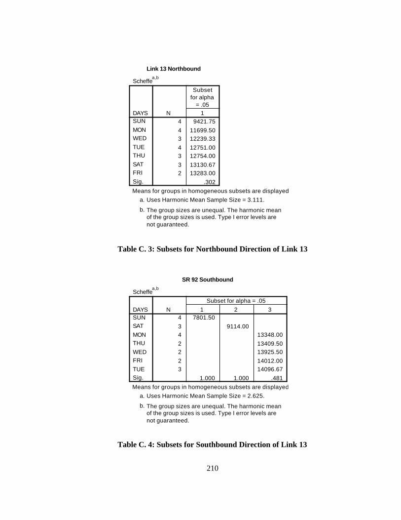
210
Link 13 Northbound
Scheffea,b
4 9421.754 11699.503 12239.334 12751.003 12754.003 13130.672 13283.00
.302
DAYSSUNMONWEDTUETHUSATFRISig.
N 1
Subsetfor alpha
= .05
Means for groups in homogeneous subsets are displayed.Uses Harmonic Mean Sample Size = 3.111.a.
The group sizes are unequal. The harmonic meanof the group sizes is used. Type I error levels arenot guaranteed.
b.
Table C. 3: Subsets for Northbound Direction of Link 13
SR 92 Southbound
Scheffea,b
4 7801.503 9114.004 13348.002 13409.502 13925.502 14012.003 14096.67
1.000 1.000 .481
DAYSSUNSATMONTHUWEDFRITUESig.
N 1 2 3Subset for alpha = .05
Means for groups in homogeneous subsets are displayed.Uses Harmonic Mean Sample Size = 2.625.a.
The group sizes are unequal. The harmonic meanof the group sizes is used. Type I error levels arenot guaranteed.
b.
Table C. 4: Subsets for Southbound Direction of Link 13

211
50th Street Southbound
Scheffea,b
5 8172.60004 9307.00002 10962.003 10977.332 11382.003 11499.002 11755.50
.326
DAYSSUNSATTHUMONFRITUEWEDSig.
N 1
Subsetfor alpha
= .05
Means for groups in homogeneous subsets are displayed.Uses Harmonic Mean Sample Size = 2.675.a.
The group sizes are unequal. The harmonic meanof the group sizes is used. Type I error levels arenot guaranteed.
b.
Table C. 5: Subsets for Southbound Direction of Link 17
50th Street Northbound
Scheffea,b
4 6864.00004 8437.25004 10089.753 10616.333 10770.673 11119.002 11224.00
1.000 1.000 .053
DAYSSUNSATMONTUEWEDTHUFRISig.
N 1 2 3Subset for alpha = .05
Means for groups in homogeneous subsets are displayed.Uses Harmonic Mean Sample Size = 3.111.a.
The group sizes are unequal. The harmonic meanof the group sizes is used. Type I error levels arenot guaranteed.
b.
Table C. 6: Subsets for Northbound Direction of Link 17

212
Causeway Eastbound
Scheffea,b
4 5371.00004 6258.7500 6258.75002 6803.5000 6803.50002 7107.50003 7542.33333 7642.00004 7837.2500
.105 .060
DAYSSUNSATMONTUEWEDTHUFRISig.
N 1 2Subset for alpha = .05
Means for groups in homogeneous subsets are displayed.Uses Harmonic Mean Sample Size = 2.897.a.
The group sizes are unequal. The harmonic meanof the group sizes is used. Type I error levels arenot guaranteed.
b.
Table C. 7: Subsets for Eastbound Direction of Link 22
Causeway Westbound
Scheffea,b
3 4855.66673 5532.66673 5819.00004 5829.75002 7469.00003 7629.33333 7850.0000
.400
DAYSSUNDAYWEDNESDAYMONDAYSATURDAYTUESDAYTHURSDAYFRIDAYSig.
N 1
Subsetfor alpha
= .05
Means for groups in homogeneous subsets are displayed.Uses Harmonic Mean Sample Size = 2.897.a.
The group sizes are unequal. The harmonic meanof the group sizes is used. Type I error levels arenot guaranteed.
b.
Table C. 8: Subsets for Westbound Direction of Link 22

213
21st Street
Scheffea,b
5 5770.20005 7087.6000 7087.60005 7277.40005 7719.00003 7782.00003 7976.00004 8235.2500
.071 .159
DAYSSUNMONSATTUEWEDTHUFRISig.
N 1 2Subset for alpha = .05
Means for groups in homogeneous subsets are displayed.Uses Harmonic Mean Sample Size = 4.078.a.
The group sizes are unequal. The harmonic meanof the group sizes is used. Type I error levels arenot guaranteed.
b.
Table C. 9: Subsets for Southbound Direction of Link 25
I-4 on-Ramp
Scheffea,b
2 1009.502 1267.502 1809.502 1842.002 1872.003 1896.003 1954.33
1.000 1.000 .121
DAYSSUNSATTUEWEDMONTHUFRISig.
N 1 2 3Subset for alpha = .05
Means for groups in homogeneous subsets are displayed.Uses Harmonic Mean Sample Size = 2.211.a.
The group sizes are unequal. The harmonic meanof the group sizes is used. Type I error levels arenot guaranteed.
b.
Table C. 10: Subsets for I-4 On-Ramp

214
SR 41
Scheffea,b
2 6594.002 8082.002 10374.002 10700.50 10700.503 10731.33 10731.332 10736.00 10736.003 11029.00
1.000 1.000 .274 .365
DAYSSUNSATWEDMONTHUTUEFRISig.
N 1 2 3 4Subset for alpha = .05
Means for groups in homogeneous subsets are displayed.Uses Harmonic Mean Sample Size = 2.211.a.
The group sizes are unequal. The harmonic mean of the groupsizes is used. Type I error levels are not guaranteed.
b.
Table C. 11: Subsets for SR 41

215
APPENDIX D Sample of CORSIM & VISSIM Traffic Assignment Output

216
8016-8015 250.0 23, 12, 17, 48, 41, 29 (SEC): .0, 27.0, 63.1, 90.1, 105.1, 122.1 T 250 VPH 8017-8012 50.0 12, 9, 19, 25, 24, 18, 1, 61 (SEC): .0, 22.0, 58.0, 72.0, 92.0, 120.0, 148.6, 162.7 50 VPH 8017-8009 150.0 12, 9, 8, 7 (SEC): .0, 22.0, 82.1, 99.1 150 VPH 8017-8002 200.0 12, 23, 30, 31, 32 (SEC): .0, 27.3, 73.2, 108.3, 134.3 200 VPH 8017-8014 12, 23, 30, 31, 32, 58, 33, 52, 14 (SEC): .0, 27.3, 73.2, 108.3, 134.9, 178.1, 227.3, 233.5, 236.6 8017-8014 12, 17, 48, 40, 35, 38, 37, 60, 33, 52, 14 (SEC): .0, 36.1, 63.1, 81.5, 88.5, 96.5, 116.5, 165.5, 226.0, 232.2, 235.3 150 VPH
Figure D. 1: A Sample of CORSIM output
Network Node Number
CORSIM Node Number
1 8007
3 8004
4 8003
5 8011
6 8010
7 8009
8 8006
9 8005
10 8017
11 8016
12 8001
13 8002
14 8014
16 8015
18 8008 Table D. 1: Network and CORSIM External Node Number
CORSIM External Nodes
CORSIM Internal Node
Volume

217
DISCHARGE ESTIMATED
LINK VOL. PCT. VOL. PCT. VOL. PCT. VOLUME SPEED
VPH VPH VPH VPH MPH
( 21, 5) 524 34 0 0 1000 66 1524 47.4
( 5, 21) 0 0 838 100 0 0 838 48.6
( 3, 2) 0 0 250 100 0 0 250 30.9
( 2, 3) 0 0 500 87 76 13 576 30.1
( 21, 2) 0 50 0 0 0 50 0 0
( 2, 21) 0 50 0 0 0 50 0 0
( 5, 4) 0 0 0 0 524 100 524 19.2
( 4, 5) 0 0 0 0 300 100 300 56.7
( 4, 3) 0 50 0 0 0 50 0 0
( 3, 4) 76 100 0 0 0 0 76 21.3
( 18, 21) 0 0 1524 100 0 0 1524 49.3
( 21, 18) 0 0 338 40 500 60 838 49.9
( 18, 1) 700 100 0 0 0 0 700 47.4
( 1, 18) 924 38 1500 62 0 0 2424 46.5
( 1, 2) 0 0 576 100 0 0 576 30.5
( 2, 1) 0 0 250 100 0 0 250 44.1
RIGHT TURN LEFT TURNTHRU
Table D. 2: A sample of CORSIM output

218
Table of Delay
No. 1:00 Travel time section(s) 1
No. 2:00 Travel time section(s) 2
No. 3:00 Travel time section(s) 3
No. 4:00 Travel time section(s) 4
No. 5:00 Travel time section(s) 5
No. 6:00 Travel time section(s) 6
No. 7:00 Travel time section(s) 7, 8
No. 8:00 Travel time section(s) 9, 10
No. 11:00 Travel time section(s) 11
No. 12:00 Travel time section(s) 12
No. 13:00 Travel time section(s) 13
No. 14:00 Travel time section(s) 14
No.
Delay; #Veh; Pers.; #Pers;
Average 34.8 91 34.8 91;
No.
Delay; #Veh; Pers.; #Pers;
18.3; 86; 18.3; 86;
Average 18.3 86 18.3 86
No.
Delay; #Veh; Pers.; #Pers;
Average 124.8 897 124.8 897
14
1
2
Figure D. 2: A Sample of VISSIM output (*.VLZ)

219
APPENDIX E CORSIM Calibration Tables Using FDOT Data

220
1 3 4 5 6 7 8 9 10 11 12 13 14 16 18
1 0 100 250 0 25 100 0 600 0 0 0 0 0 0 150
3 100 0 500 0 0 0 500 250 0 0 0 0 0 0 04 0 500 0 0 0 0 0 0 0 0 0 0 0 0 200
5 0 0 0 0 0 0 0 0 0 0 0 0 0 0 150
6 40 0 0 0 0 0 0 250 100 0 400 0 0 350 07 0 0 0 0 0 0 0 500 150 0 1300 0 0 0 50
8 0 0 0 0 0 0 0 0 0 0 0 0 0 350 09 700 0 350 0 850 50 0 0 0 0 1000 0 50 150 0
10 50 0 0 0 500 150 0 0 0 0 0 100 100 300 0
11 0 0 0 0 0 0 0 0 0 0 300 0 0 250 012 0 0 0 0 300 500 0 100 0 150 0 0 450 0 0
13 0 0 0 0 0 0 0 0 50 0 0 0 0 120 0
14 0 0 0 0 0 0 0 500 200 400 0 0 200 016 0 0 0 0 0 0 100 100 250 200 50 100 350 0 0
18 350 100 250 100 0 50 50 150 0 0 0 0 0 0 0
Figure E. 1: The 13th Iteration O-D Matrix
FDOT Data Simulated Data % error FDOT Data Simulated Data % errorL-14 570 540 5.62 488 675 27.78L-20 493 574 14.20 578 607 4.70L-23 928 810 14.58 1089 1219 10.63L-24 1011 678 49.24 861 680 26.71L-25 830 817 1.54 573 679 15.68L-30 983 744 32.15 856 801 6.87
Inbound Outbound
Table E. 1: FDOT and CORSIM Simulated Volumes for the Master Links (13th
Iteration)

221
1 3 4 5 6 7 8 9 10 11 12 13 14 16 18
1 0 100 250 0 25 100 0 600 0 0 0 0 0 0 150
3 100 0 500 0 0 0 500 250 0 0 0 0 0 0 04 0 500 0 0 0 0 0 0 0 0 0 0 0 0 200
5 0 0 0 0 0 0 0 0 0 0 0 0 0 0 250
6 40 0 0 0 0 0 0 250 100 0 400 0 0 0 07 0 0 0 0 0 0 0 500 300 0 1300 0 0 0 350
8 0 0 0 0 0 0 0 0 0 0 0 0 0 250 1009 700 0 350 0 850 50 0 0 0 0 1000 0 50 150 0
10 50 0 0 0 500 150 0 0 0 0 0 100 100 300 0
11 0 0 0 0 0 0 0 0 0 0 300 0 0 250 012 0 0 0 0 300 500 0 100 0 150 0 0 450 0 0
13 0 0 0 0 0 0 0 0 50 0 0 0 0 50 0
14 0 0 0 0 0 0 0 500 50 0 400 0 0 600 016 0 0 0 0 0 0 100 100 250 200 50 100 350 0 0
18 350 100 250 100 0 50 50 150 0 0 0 0 0 0 0
Figure E. 2: The O-D Matrix of the 14th Iteration
FDOT Data Simulated Data % error FDOT Data Simulated Data % errorL-14 570 541 5.52 488 675 27.78L-20 493 585 15.81 578 631 8.40L-23 928 800 16.01 1089 1254 13.12L-24 1011 755 34.01 861 734 17.38L-25 830 850 2.40 573 685 16.42L-30 983 1076 8.69 856 887 3.55
Inbound Outbound
Table E. 2: FDOT and CORSIM Simulated Volumes for the Master Links (14th Iteration)
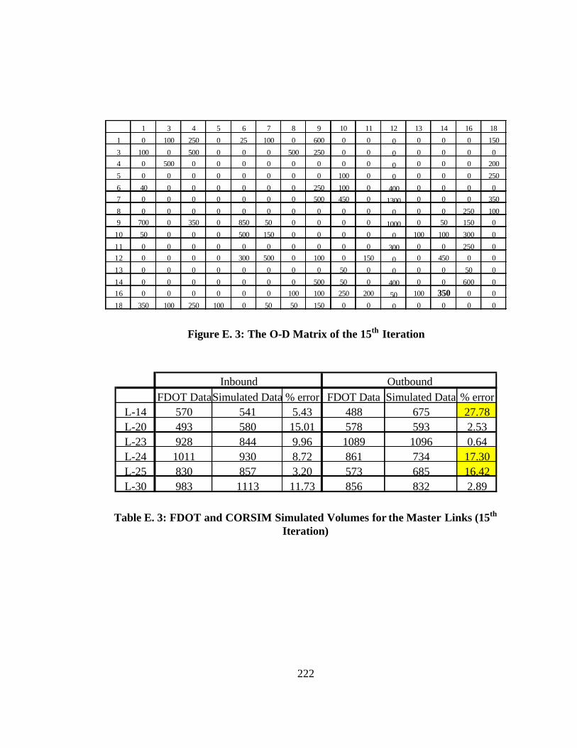
222
1 3 4 5 6 7 8 9 10 11 12 13 14 16 18
1 0 100 250 0 25 100 0 600 0 0 0 0 0 0 150
3 100 0 500 0 0 0 500 250 0 0 0 0 0 0 04 0 500 0 0 0 0 0 0 0 0 0 0 0 0 200
5 0 0 0 0 0 0 0 0 100 0 0 0 0 0 250
6 40 0 0 0 0 0 0 250 100 0 400 0 0 0 07 0 0 0 0 0 0 0 500 450 0 1300 0 0 0 350
8 0 0 0 0 0 0 0 0 0 0 0 0 0 250 1009 700 0 350 0 850 50 0 0 0 0 1000 0 50 150 0
10 50 0 0 0 500 150 0 0 0 0 0 100 100 300 0
11 0 0 0 0 0 0 0 0 0 0 300 0 0 250 012 0 0 0 0 300 500 0 100 0 150 0 0 450 0 0
13 0 0 0 0 0 0 0 0 50 0 0 0 0 50 0
14 0 0 0 0 0 0 0 500 50 0 400 0 0 600 016 0 0 0 0 0 0 100 100 250 200 50 100 350 0 0
18 350 100 250 100 0 50 50 150 0 0 0 0 0 0 0
Figure E. 3: The O-D Matrix of the 15th Iteration
FDOT DataSimulated Data % error FDOT Data Simulated Data % errorL-14 570 541 5.43 488 675 27.78L-20 493 580 15.01 578 593 2.53L-23 928 844 9.96 1089 1096 0.64L-24 1011 930 8.72 861 734 17.30L-25 830 857 3.20 573 685 16.42L-30 983 1113 11.73 856 832 2.89
Inbound Outbound
Table E. 3: FDOT and CORSIM Simulated Volumes for the Master Links (15th Iteration)
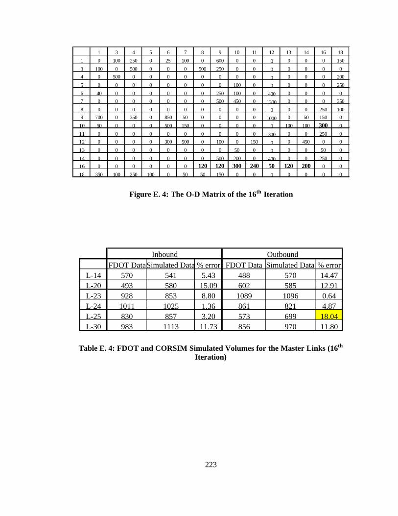
223
1 3 4 5 6 7 8 9 10 11 12 13 14 16 18
1 0 100 250 0 25 100 0 600 0 0 0 0 0 0 150
3 100 0 500 0 0 0 500 250 0 0 0 0 0 0 04 0 500 0 0 0 0 0 0 0 0 0 0 0 0 200
5 0 0 0 0 0 0 0 0 100 0 0 0 0 0 250
6 40 0 0 0 0 0 0 250 100 0 400 0 0 0 07 0 0 0 0 0 0 0 500 450 0 1300 0 0 0 350
8 0 0 0 0 0 0 0 0 0 0 0 0 0 250 1009 700 0 350 0 850 50 0 0 0 0 1000 0 50 150 0
10 50 0 0 0 500 150 0 0 0 0 0 100 100 300 0
11 0 0 0 0 0 0 0 0 0 0 300 0 0 250 012 0 0 0 0 300 500 0 100 0 150 0 0 450 0 0
13 0 0 0 0 0 0 0 0 50 0 0 0 0 50 0
14 0 0 0 0 0 0 0 500 200 0 400 0 0 250 016 0 0 0 0 0 0 120 120 300 240 50 120 200 0 0
18 350 100 250 100 0 50 50 150 0 0 0 0 0 0 0
Figure E. 4: The O-D Matrix of the 16th Iteration
FDOT DataSimulated Data % error FDOT Data Simulated Data % errorL-14 570 541 5.43 488 570 14.47L-20 493 580 15.09 602 585 12.91L-23 928 853 8.80 1089 1096 0.64L-24 1011 1025 1.36 861 821 4.87L-25 830 857 3.20 573 699 18.04L-30 983 1113 11.73 856 970 11.80
Inbound Outbound
Table E. 4: FDOT and CORSIM Simulated Volumes for the Master Links (16th Iteration)

224
1 3 4 5 6 7 8 9 10 11 12 13 14 16 18
1 0 100 250 0 25 100 0 600 0 0 0 0 0 0 150
3 100 0 500 0 0 0 500 250 0 0 0 0 0 0 04 0 500 0 0 0 0 0 0 0 0 0 0 0 0 200
5 0 0 0 0 0 0 0 0 100 0 0 0 0 0 250
6 40 0 0 0 0 0 0 250 450 0 400 0 0 0 07 0 0 0 0 0 0 0 500 0 0 1300 0 0 0 350
8 0 0 0 0 0 0 0 0 0 0 0 0 0 290 1009 700 350 0 0 850 50 0 0 0 0 1000 0 50 175 0
10 50 0 0 0 500 150 0 0 0 0 0 100 100 150 0
11 0 0 0 0 0 0 0 0 0 0 300 0 0 290 012 0 0 0 0 300 500 0 100 0 150 0 0 450 0 0
13 0 0 0 0 0 0 0 0 50 0 0 0 0 58 0
14 0 0 0 0 0 0 0 500 200 0 400 0 0 290 016 0 0 0 0 0 0 120 120 300 240 50 120 200 0 0
18 350 100 250 100 0 50 50 150 0 0 0 0 0 0 0
Figure E. 5: The O-D Matrix of the 17th Iteration
FDOT DataSimulated Data % error FDOT Data Simulated Data % errorL-14 570 541 5.43 488 570 14.47L-20 537 470 14.26 602 653 7.74L-23 928 810 14.51 1089 1003 8.57L-24 1011 899 12.53 861 808 6.63L-25 830 882 5.89 573 607 5.68L-30 983 985 0.25 856 988 13.41
Inbound Outbound
Table E. 5: FDOT and CORSIM Simulated Volumes for the Master Links (17th Iteration)

225
APPENDIX F Output of the Truck Trip Generation ANN Model from
Phase II for the Port of Tampa
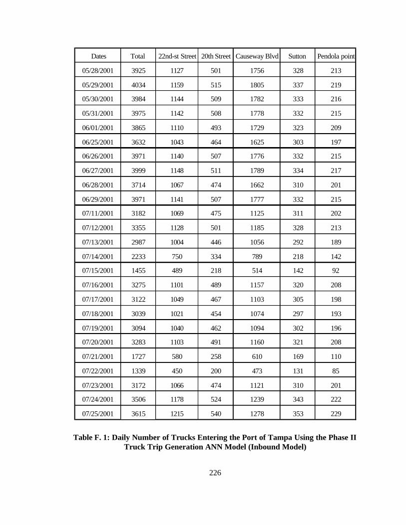
226
Dates Total 22nd-st Street 20th Street Causeway Blvd Sutton Pendola point
05/28/2001 3925 1127 501 1756 328 213
05/29/2001 4034 1159 515 1805 337 219
05/30/2001 3984 1144 509 1782 333 216
05/31/2001 3975 1142 508 1778 332 215
06/01/2001 3865 1110 493 1729 323 209
06/25/2001 3632 1043 464 1625 303 197
06/26/2001 3971 1140 507 1776 332 215
06/27/2001 3999 1148 511 1789 334 217
06/28/2001 3714 1067 474 1662 310 201
06/29/2001 3971 1141 507 1777 332 215
07/11/2001 3182 1069 475 1125 311 202
07/12/2001 3355 1128 501 1185 328 213
07/13/2001 2987 1004 446 1056 292 189
07/14/2001 2233 750 334 789 218 142
07/15/2001 1455 489 218 514 142 92
07/16/2001 3275 1101 489 1157 320 208
07/17/2001 3122 1049 467 1103 305 198
07/18/2001 3039 1021 454 1074 297 193
07/19/2001 3094 1040 462 1094 302 196
07/20/2001 3283 1103 491 1160 321 208
07/21/2001 1727 580 258 610 169 110
07/22/2001 1339 450 200 473 131 85
07/23/2001 3172 1066 474 1121 310 201
07/24/2001 3506 1178 524 1239 343 222
07/25/2001 3615 1215 540 1278 353 229
Table F. 1: Daily Number of Trucks Entering the Port of Tampa Using the Phase II Truck Trip Generation ANN Model (Inbound Model)
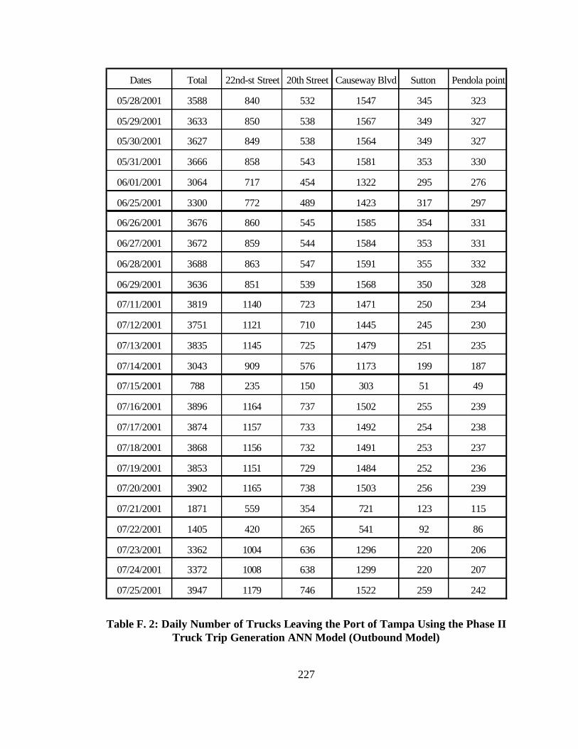
227
Dates Total 22nd-st Street 20th Street Causeway Blvd Sutton Pendola point
05/28/2001 3588 840 532 1547 345 323
05/29/2001 3633 850 538 1567 349 327
05/30/2001 3627 849 538 1564 349 327
05/31/2001 3666 858 543 1581 353 330
06/01/2001 3064 717 454 1322 295 276
06/25/2001 3300 772 489 1423 317 297
06/26/2001 3676 860 545 1585 354 331
06/27/2001 3672 859 544 1584 353 331
06/28/2001 3688 863 547 1591 355 332
06/29/2001 3636 851 539 1568 350 328
07/11/2001 3819 1140 723 1471 250 234
07/12/2001 3751 1121 710 1445 245 230
07/13/2001 3835 1145 725 1479 251 235
07/14/2001 3043 909 576 1173 199 187
07/15/2001 788 235 150 303 51 49
07/16/2001 3896 1164 737 1502 255 239
07/17/2001 3874 1157 733 1492 254 238
07/18/2001 3868 1156 732 1491 253 237
07/19/2001 3853 1151 729 1484 252 236
07/20/2001 3902 1165 738 1503 256 239
07/21/2001 1871 559 354 721 123 115
07/22/2001 1405 420 265 541 92 86
07/23/2001 3362 1004 636 1296 220 206
07/24/2001 3372 1008 638 1299 220 207
07/25/2001 3947 1179 746 1522 259 242
Table F. 2: Daily Number of Trucks Leaving the Port of Tampa Using the Phase II Truck Trip Generation ANN Model (Outbound Model)

228
APPENDIX G Final Calibration Tables for CORSIM and
Field Calibrated O-D Matrices
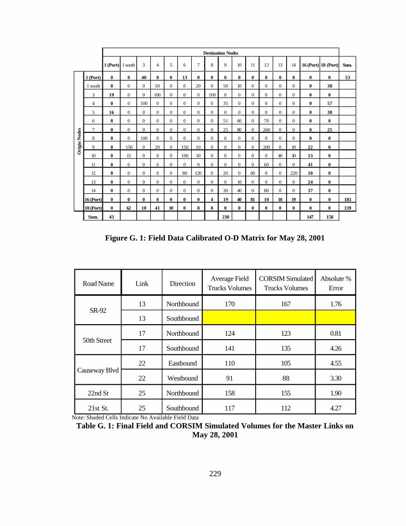
229
1 (Port) 1 south 3 4 5 6 7 8 9 10 11 12 13 14 16 (Port) 18 (Port) Sum.
1 (Port) 0 0 40 0 0 13 0 0 0 0 0 0 0 0 0 0 53
1 south 0 0 0 50 0 0 20 0 50 10 0 0 0 0 0 38
3 19 0 0 100 0 0 0 100 0 0 0 0 0 0 0 0
4 0 0 100 0 0 0 0 0 35 0 0 0 0 0 0 57
5 16 0 0 0 0 0 0 0 0 0 0 0 0 0 0 38
6 8 0 0 0 0 0 0 0 51 60 0 70 0 0 0 0
7 0 0 0 0 0 0 0 0 25 80 0 260 0 0 0 25
8 0 0 100 0 0 0 0 0 0 0 0 0 0 0 0 0
9 0 150 0 20 0 150 10 0 0 0 0 200 0 10 22 0
10 0 15 0 0 0 100 30 0 0 0 0 0 40 30 13 0
11 0 0 0 0 0 0 0 0 0 0 0 60 0 0 41 0
12 0 0 0 0 0 80 120 0 20 0 60 0 0 220 10 0
13 0 0 0 0 0 0 0 0 0 10 0 0 0 0 24 0
14 0 0 0 0 0 0 0 0 30 40 0 80 0 0 37 0
16 (Port) 0 0 0 0 0 0 0 4 19 40 81 10 10 19 0 0 183
18 (Port) 0 62 10 41 10 0 8 8 0 0 0 0 0 0 0 0 139
Sum. 43 230 147 158
Destination Nodes
Ori
gin
Nod
es
Figure G. 1: Field Data Calibrated O-D Matrix for May 28, 2001
Road Name Link DirectionAverage Field
Trucks VolumesCORSIM Simulated
Trucks VolumesAbsolute %
Error
13 Northbound 170 167 1.76
13 Southbound
17 Northbound 124 123 0.81
17 Southbound 141 135 4.26
22 Eastbound 110 105 4.55
22 Westbound 91 88 3.30
22nd St 25 Northbound 158 155 1.90
21st St. 25 Southbound 117 112 4.27
SR-92
50th Street
Causeway Blvd
Note: Shaded Cells Indicate No Available Field Data
Table G. 1: Final Field and CORSIM Simulated Volumes for the Master Links on May 28, 2001

230
1 (Port) 1 south 3 4 5 6 7 8 9 10 11 12 13 14 16 (Port) 18 (Port) Sum.
1 (Port) 0 0 41 0 0 13 0 0 0 0 0 0 0 0 0 0 54
1 south 0 0 0 50 0 0 20 0 50 10 0 0 0 0 0 39
3 20 0 0 100 0 0 0 100 0 0 0 0 0 0 0 0
4 0 0 100 0 0 0 0 0 35 0 0 0 0 0 0 59
5 16 0 0 0 0 0 0 0 0 0 0 0 0 0 0 39
6 8 0 0 0 0 0 0 0 51 60 0 70 0 0 0 0
7 0 0 0 0 0 0 0 0 25 80 0 260 0 0 0 25
8 0 0 100 0 0 0 0 0 0 0 0 0 0 0 0 0
9 0 130 0 20 0 150 10 0 0 0 0 200 0 10 24 0
10 0 17 0 0 0 100 30 0 0 0 0 0 40 30 13 0
11 0 0 0 0 0 0 0 0 0 0 0 60 0 0 42 0
12 0 0 0 0 0 80 120 0 20 0 60 0 0 220 10 0
13 0 0 0 0 0 0 0 0 0 10 0 0 0 0 24 0
14 0 0 0 0 0 0 0 0 30 40 0 65 0 0 38 0
16 (Port) 0 0 0 0 0 0 0 4 19 41 82 10 10 19 0 0 185
18 (Port) 0 63 10 42 10 0 8 8 0 0 0 0 0 0 0 0 141
Sum. 44 230 151 162
Destination Nodes
Ori
gin
Nod
es
Figure G. 2: Field Data Calibrated O-D Matrix for May 29, 2001
Road Name Link DirectionAverage Field
Trucks VolumesCORSIM Simulated
Trucks VolumesAbsolute %
Error
13 Northbound 154 157 1.95
13 Southbound
17 Northbound 120 124 3.33
17 Southbound 115 114 0.87
22 Eastbound 91 94 3.30
22 Westbound 85 89 4.71
22nd St 25 Northbound 159 155 2.52
21st St. 25 Southbound 118 113 4.24
SR-92
50th Street
Causeway Blvd
Note: Shaded Cells Indicate No Available Field Data
Table G. 2: Final Field and CORSIM Simulated Volumes for the Master Links on May 29, 2001
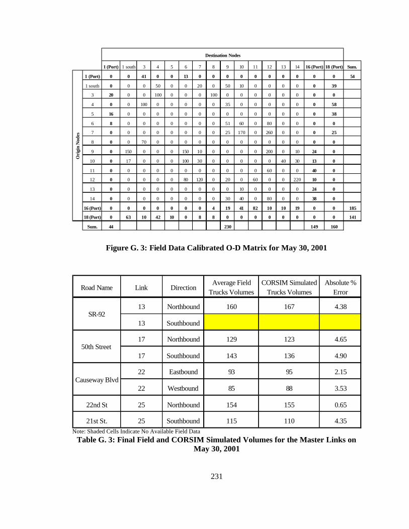
231
1 (Port) 1 south 3 4 5 6 7 8 9 10 11 12 13 14 16 (Port) 18 (Port) Sum.
1 (Port) 0 0 41 0 0 13 0 0 0 0 0 0 0 0 0 0 54
1 south 0 0 0 50 0 0 20 0 50 10 0 0 0 0 0 39
3 20 0 0 100 0 0 0 100 0 0 0 0 0 0 0 0
4 0 0 100 0 0 0 0 0 35 0 0 0 0 0 0 58
5 16 0 0 0 0 0 0 0 0 0 0 0 0 0 0 38
6 8 0 0 0 0 0 0 0 51 60 0 80 0 0 0 0
7 0 0 0 0 0 0 0 0 25 170 0 260 0 0 0 25
8 0 0 70 0 0 0 0 0 0 0 0 0 0 0 0 0
9 0 150 0 0 0 150 10 0 0 0 0 200 0 10 24 0
10 0 17 0 0 0 100 30 0 0 0 0 0 40 30 13 0
11 0 0 0 0 0 0 0 0 0 0 0 60 0 0 40 0
12 0 0 0 0 0 80 120 0 20 0 60 0 0 220 10 0
13 0 0 0 0 0 0 0 0 0 10 0 0 0 0 24 0
14 0 0 0 0 0 0 0 0 30 40 0 80 0 0 38 0
16 (Port) 0 0 0 0 0 0 0 4 19 41 82 10 10 19 0 0 185
18 (Port) 0 63 10 42 10 0 8 8 0 0 0 0 0 0 0 0 141
Sum. 44 230 149 160
Destination Nodes
Ori
gin
Nod
es
Figure G. 3: Field Data Calibrated O-D Matrix for May 30, 2001
Road Name Link DirectionAverage Field
Trucks VolumesCORSIM Simulated
Trucks VolumesAbsolute %
Error
13 Northbound 160 167 4.38
13 Southbound
17 Northbound 129 123 4.65
17 Southbound 143 136 4.90
22 Eastbound 93 95 2.15
22 Westbound 85 88 3.53
22nd St 25 Northbound 154 155 0.65
21st St. 25 Southbound 115 110 4.35
SR-92
50th Street
Causeway Blvd
Note: Shaded Cells Indicate No Available Field Data
Table G. 3: Final Field and CORSIM Simulated Volumes for the Master Links on May 30, 2001

232
1 (Port) 1 south 3 4 5 6 7 8 9 10 11 12 13 14 16 (Port) 18 (Port) Sum.
1 (Port) 0 0 42 0 0 13 0 0 0 0 0 0 0 0 0 0 55
1 south 0 0 0 50 0 0 20 0 55 10 0 0 0 0 0 39
3 20 0 0 100 0 0 0 100 0 0 0 0 0 0 0 0
4 0 0 100 0 0 0 0 0 30 0 0 0 0 0 0 58
5 16 0 0 0 0 0 0 0 0 0 0 0 0 0 0 38
6 8 0 0 0 0 0 0 0 50 60 0 80 0 0 0 0
7 0 0 0 0 0 0 0 0 26 170 0 260 0 0 0 25
8 0 0 70 0 0 0 0 0 0 0 0 0 0 0 0 0
9 0 145 0 0 0 150 10 0 0 0 0 200 0 10 24 0
10 0 10 0 0 0 100 30 0 0 0 0 0 40 30 15 0
11 0 0 0 0 0 0 0 0 0 0 0 60 0 0 38 0
12 0 0 0 0 0 80 120 0 20 0 60 0 0 220 10 0
13 0 0 0 0 0 0 0 0 0 10 0 0 0 0 24 0
14 0 0 0 0 0 0 0 0 30 40 0 80 0 0 38 0
16 (Port) 0 0 0 0 0 0 0 4 19 42 83 10 10 19 0 0 187
18 (Port) 0 64 10 42 10 0 8 8 0 0 0 0 0 0 0 0 142
Sum. 44 230 149 160
Destination Nodes
Ori
gin
Nod
es
Figure G. 4: The Field Data Calibrated O-D Matrix for May 31, 2001
Road Name Link DirectionAverage Field
Trucks VolumesCORSIM Simulated
Trucks Volumes% Error
13 Northbound 169 167 1.18
13 Southbound
17 Northbound 132 128 3.03
17 Southbound 134 130 2.99
22 Eastbound 95 95 0.00
22 Westbound 87 88 1.15
22nd St 25 Northbound 150 155 3.33
21st St. 25 Southbound 119 114 4.20
SR-92
50th Street
Causeway Blvd
Note: Shaded Cells Indicate No Available Field Data
Table G. 4: Final Field and CORSIM Simulated Volumes for the Master Links on May 31, 2001

233
1 (Port) 1 south 3 4 5 6 7 8 9 10 11 12 13 14 16 (Port) 18 (Port) Sum.
1 (Port) 0 0 34 0 0 12 0 0 0 0 0 0 0 0 0 0 46
1 south 0 0 0 50 0 0 20 0 55 10 0 0 0 0 0 38
3 20 0 0 100 0 0 0 100 0 0 0 0 0 0 0 0
4 0 0 100 0 0 0 0 0 30 0 0 0 0 0 0 56
5 15 0 0 0 0 0 0 0 0 0 0 0 0 0 0 37
6 8 0 0 0 0 0 0 0 50 60 0 80 0 0 0 0
7 0 0 0 0 0 0 0 0 29 170 0 260 0 0 0 25
8 0 0 70 0 0 0 0 0 0 0 0 0 0 0 0 0
9 0 155 0 0 0 150 10 0 0 0 0 200 0 10 26 0
10 0 17 0 0 0 100 30 0 0 0 0 0 40 30 13 0
11 0 0 0 0 0 0 0 0 0 0 0 60 0 0 40 0
12 0 0 0 0 0 80 120 0 20 0 60 0 0 220 10 0
13 0 0 0 0 0 0 0 0 0 10 0 0 0 0 20 0
14 0 0 0 0 0 0 0 0 30 40 0 80 0 0 35 0
16 (Port) 0 0 0 0 0 0 0 6 16 34 70 8 8 14 0 0 156
18 (Port) 0 50 9 35 9 0 8 8 0 0 0 0 0 0 0 0 119
Sum. 43 230 144 156
Destination Nodes
Ori
gin
Nod
es
Figure G. 5: Field Data Calibrated O-D Matrix for June 1, 2001
Road Name Link DirectionAverage Field
Trucks VolumesCORSIM Simulated
Trucks Volumes% Error
13 Northbound 177 169 4.52
13 Southbound
17 Northbound 134 128 4.83
17 Southbound 145 138 4.04
22 Eastbound 99 95 3.30
22 Westbound 91 88 4.17
22nd St 25 Northbound
21st St. 25 Southbound 120 115 4.17
SR-92
50th Street
Causeway Blvd
Note: Shaded Cells Indicate No Available Field Data
Table G. 5: Final Field and CORSIM Simulated Volumes for the Master Links on June 1, 2001

234
1 (Port) 1 south 3 4 5 6 7 8 9 10 11 12 13 14 16 (Port) 18 (Port) Sum.
1 (Port) 0 0 36 0 0 13 0 0 0 0 0 0 0 0 0 0 49
1 south 0 0 0 50 0 0 20 0 50 10 0 0 0 0 0 35
3 19 0 0 100 0 0 0 100 0 0 0 0 0 0 0 0
4 0 0 100 0 0 0 0 0 35 0 0 0 0 0 0 53
5 15 0 0 0 0 0 0 0 0 0 0 0 0 0 0 35
6 6 0 0 0 0 0 0 0 52 60 0 80 0 0 0 0
7 0 0 0 0 0 0 0 0 25 170 0 260 0 0 0 23
8 0 0 70 0 0 0 0 0 0 0 0 0 0 0 0 0
9 0 140 0 0 0 150 10 0 0 0 0 200 0 10 21 0
10 0 18 0 0 0 100 30 0 0 0 0 0 40 30 8 0
11 0 0 0 0 0 0 0 0 0 0 0 60 0 0 39 0
12 0 0 0 0 0 80 120 0 20 0 60 0 0 210 8 0
13 0 0 0 0 0 0 0 0 0 10 0 0 0 0 22 0
14 0 0 0 0 0 0 0 0 30 40 0 85 0 0 38 0
16 (Port) 0 0 0 0 0 0 0 8 18 30 74 10 10 18 0 0 168
18 (Port) 0 56 9 38 9 0 8 8 0 0 0 0 0 0 0 0 128
Sum. 40 230 136 146
Destination Nodes
Ori
gin
Nod
es
Figure G. 6: Field Data Calibrated O-D Matrix for June 25, 2001
Road Name Link DirectionAverage Field
Trucks VolumesCORSIM Simulated
Trucks Volumes% Error
13 Northbound 179 172 3.91
13 Southbound 165 169 2.42
17 Northbound 126 123 2.38
17 Southbound
22 Eastbound 93 95 2.15
22 Westbound 87 88 1.15
22nd St 25 Northbound 142 148 4.23
21st St. 25 Southbound 112 108 3.57
SR-92
50th Street
Causeway Blvd
Note: Shaded Cells Indicate No Available Field Data
Table G. 6: Final Field and CORSIM Simulated Volumes for the Master Links on June 25, 2001
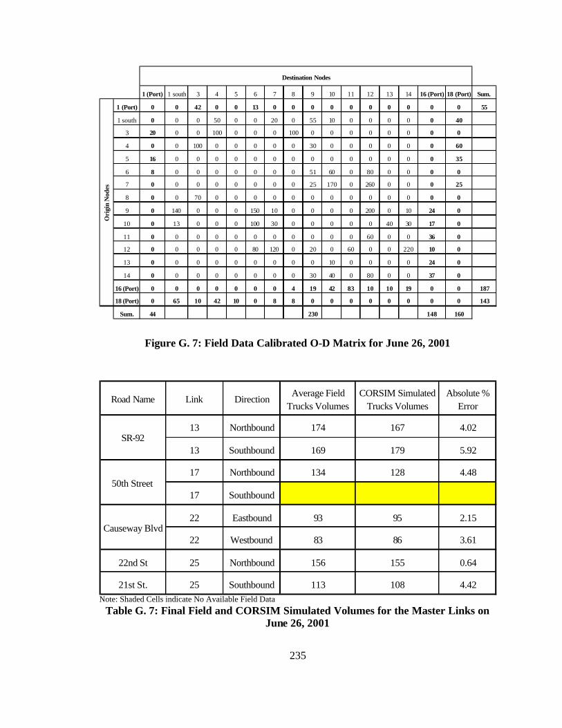
235
1 (Port) 1 south 3 4 5 6 7 8 9 10 11 12 13 14 16 (Port) 18 (Port) Sum.
1 (Port) 0 0 42 0 0 13 0 0 0 0 0 0 0 0 0 0 55
1 south 0 0 0 50 0 0 20 0 55 10 0 0 0 0 0 40
3 20 0 0 100 0 0 0 100 0 0 0 0 0 0 0 0
4 0 0 100 0 0 0 0 0 30 0 0 0 0 0 0 60
5 16 0 0 0 0 0 0 0 0 0 0 0 0 0 0 35
6 8 0 0 0 0 0 0 0 51 60 0 80 0 0 0 0
7 0 0 0 0 0 0 0 0 25 170 0 260 0 0 0 25
8 0 0 70 0 0 0 0 0 0 0 0 0 0 0 0 0
9 0 140 0 0 0 150 10 0 0 0 0 200 0 10 24 0
10 0 13 0 0 0 100 30 0 0 0 0 0 40 30 17 0
11 0 0 0 0 0 0 0 0 0 0 0 60 0 0 36 0
12 0 0 0 0 0 80 120 0 20 0 60 0 0 220 10 0
13 0 0 0 0 0 0 0 0 0 10 0 0 0 0 24 0
14 0 0 0 0 0 0 0 0 30 40 0 80 0 0 37 0
16 (Port) 0 0 0 0 0 0 0 4 19 42 83 10 10 19 0 0 187
18 (Port) 0 65 10 42 10 0 8 8 0 0 0 0 0 0 0 0 143
Sum. 44 230 148 160
Destination Nodes
Ori
gin
Nod
es
Figure G. 7: Field Data Calibrated O-D Matrix for June 26, 2001
Road Name Link DirectionAverage Field
Trucks VolumesCORSIM Simulated
Trucks VolumesAbsolute %
Error
13 Northbound 174 167 4.02
13 Southbound 169 179 5.92
17 Northbound 134 128 4.48
17 Southbound
22 Eastbound 93 95 2.15
22 Westbound 83 86 3.61
22nd St 25 Northbound 156 155 0.64
21st St. 25 Southbound 113 108 4.42
Causeway Blvd
SR-92
50th Street
Note: Shaded Cells indicate No Available Field Data
Table G. 7: Final Field and CORSIM Simulated Volumes for the Master Links on June 26, 2001

236
1 (Port) 1 south 3 4 5 6 7 8 9 10 11 12 13 14 16 (Port) 18 (Port) Sum.
1 (Port) 0 0 42 0 0 13 0 0 0 0 0 0 0 0 0 0 55
1 south 0 0 0 50 0 0 20 0 55 10 0 0 0 0 0 40
3 20 0 0 100 0 0 0 100 0 0 0 0 0 0 0 0
4 0 0 100 0 0 0 0 0 30 0 0 0 0 0 0 61
5 16 0 0 0 0 0 0 0 0 0 0 0 0 0 0 35
6 8 0 0 0 0 0 0 0 51 60 0 80 0 0 0 0
7 0 0 0 0 0 0 0 0 25 170 0 260 0 0 0 25
8 0 0 70 0 0 0 0 0 0 0 0 0 0 0 0 0
9 0 140 0 0 0 150 10 0 0 0 0 200 0 10 24 0
10 0 13 0 0 0 100 30 0 0 0 0 0 40 30 20 0
11 0 0 0 0 0 0 0 0 0 0 0 60 0 0 37 0
12 0 0 0 0 0 80 120 0 20 0 60 0 0 210 10 0
13 0 0 0 0 0 0 0 0 0 10 0 0 0 0 23 0
14 0 0 0 0 0 0 0 0 30 40 0 80 0 0 35 0
16 (Port) 0 0 0 0 0 0 0 4 19 42 83 10 10 19 0 0 187
18 (Port) 0 65 10 42 10 0 8 8 0 0 0 0 0 0 0 0 143
Sum. 44 230 149 161
Destination Nodes
Ori
gin
Nod
es
Figure G. 8: Field Data Calibrated O-D Matrix for June 27, 2001
Road Name Link DirectionAverage Field
Trucks VolumesCORSIM Simulated
Trucks VolumesAbsolute %
Error
13 Northbound 159 166 4.40
13 Southbound 163 170 4.29
17 Northbound 132 128 3.03
17 Southbound
22 Eastbound 94 95 1.06
22 Westbound 89 88 1.12
22nd St 25 Northbound 158 155 1.90
21st St. 25 Southbound 114 109 4.39
SR-92
50th Street
Causeway Blvd
Note: Shaded Cells Indicate No Available Field Data
Table G. 8: Final Field and CORSIM Simulated Volumes for the Master Links on June 27, 2001

237
1 (Port) 1 south 3 4 5 6 7 8 9 10 11 12 13 14 16 (Port) 18 (Port) Sum.
1 (Port) 0 0 42 0 0 13 0 0 0 0 0 0 0 0 0 0 55
1 south 0 0 0 50 0 0 20 0 55 10 0 0 0 0 0 36
3 20 0 0 100 0 0 0 100 0 0 0 0 0 0 0 0
4 0 0 100 0 0 0 0 0 30 0 0 0 0 0 0 54
5 15 0 0 0 0 0 0 0 0 0 0 0 0 0 0 36
6 6 0 0 0 0 0 0 0 51 60 0 80 0 0 0 0
7 0 0 0 0 0 0 0 0 25 170 0 260 0 0 0 24
8 0 0 70 0 0 0 0 0 0 0 0 0 0 0 0 0
9 0 140 0 0 0 150 10 0 0 0 0 200 0 10 24 0
10 0 13 0 0 0 100 30 0 0 0 0 0 40 30 24 0
11 0 0 0 0 0 0 0 0 0 0 0 60 0 0 36 0
12 0 0 0 0 0 80 120 0 20 0 60 0 0 210 10 0
13 0 0 0 0 0 0 0 0 0 10 0 0 0 0 23 0
14 0 0 0 0 0 0 0 0 30 40 0 80 0 0 32 0
16 (Port) 0 0 0 0 0 0 0 4 19 42 84 10 10 19 0 0 188
18 (Port) 0 65 10 42 10 0 8 8 0 0 0 0 0 0 0 0 143
Sum. 41 230 149 150
Destination Nodes
Ori
gin
Nod
es
Figure G. 9: Field Data Calibrated O-D Matrix for June 28, 2001
Road Name Link DirectionAverage Field
Trucks VolumesCORSIM Simulated
Trucks VolumesAbsolute %
Error
13 Northbound 167 165 1.20
13 Southbound 161 169 4.97
17 Northbound 134 128 4.48
17 Southbound
22 Eastbound 98 95 3.06
22 Westbound 90 88 2.22
22nd St 25 Northbound 153 155 1.31
21st St. 25 Southbound 114 109 4.39
SR-92
50th Street
Causeway Blvd
Note: Shaded Cells Indicate No Available Field Data
Table G. 9: Final Field and CORSIM Simulated Volumes for the Master Links on June 28, 2001

238
1 (Port) 1 south 3 4 5 6 7 8 9 10 11 12 13 14 16 (Port) 18 (Port) Sum.
1 (Port) 0 0 41 0 0 13 0 0 0 0 0 0 0 0 0 0 54
1 south 0 0 0 50 0 0 20 0 55 10 0 0 0 0 0 41
3 20 0 0 100 0 0 0 100 0 0 0 0 0 0 0 0
4 0 0 100 0 0 0 0 0 30 0 0 0 0 0 0 62
5 16 0 0 0 0 0 0 0 0 0 0 0 0 0 0 32
6 8 0 0 0 0 0 0 0 51 60 0 80 0 0 0 0
7 0 0 0 0 0 0 0 0 25 170 0 260 0 0 0 25
8 0 0 70 0 0 0 0 0 0 0 0 0 0 0 0 0
9 0 140 0 0 0 150 10 0 0 0 0 200 0 10 24 0
10 0 15 0 0 0 100 30 0 0 0 0 0 40 30 27 0
11 0 0 0 0 0 0 0 0 0 0 0 60 0 0 34 0
12 0 0 0 0 0 80 120 0 20 0 60 0 0 210 10 0
13 0 0 0 0 0 0 0 0 0 10 0 0 0 0 23 0
14 0 0 0 0 0 0 0 0 30 40 0 80 0 0 30 0
16 (Port) 0 0 0 0 0 0 0 4 19 42 81 10 10 19 0 0 185
18 (Port) 0 64 10 41 10 0 8 8 0 0 0 0 0 0 0 0 141
Sum. 44 230 148 160
Destination Nodes
Ori
gin
Nod
es
Figure G. 10: Field Data Calibrated O-D Matrix for June 29, 2001
Road Name Link DirectionAverage Field
Trucks VolumesCORSIM Simulated
Trucks VolumesAbsolute %
Error
13 Northbound 167 168 0.60
13 Southbound 161 169 4.97
17 Northbound 134 128 4.48
17 Southbound
22 Eastbound 99 95 4.04
22 Westbound 80 84 5.00
22nd St 25 Northbound 159 155 2.52
21st St. 25 Southbound 120 115 4.17
50th Street
Causeway Blvd
SR-92
Note: Shaded Cells Indicate No Available Field Data
Table G. 10: Table G.10 Final Field and CORSIM Simulated Volumes for the Master Links on June 29, 2001

239
APPENDIX H C.I. Method for CORSIM Models Calibration
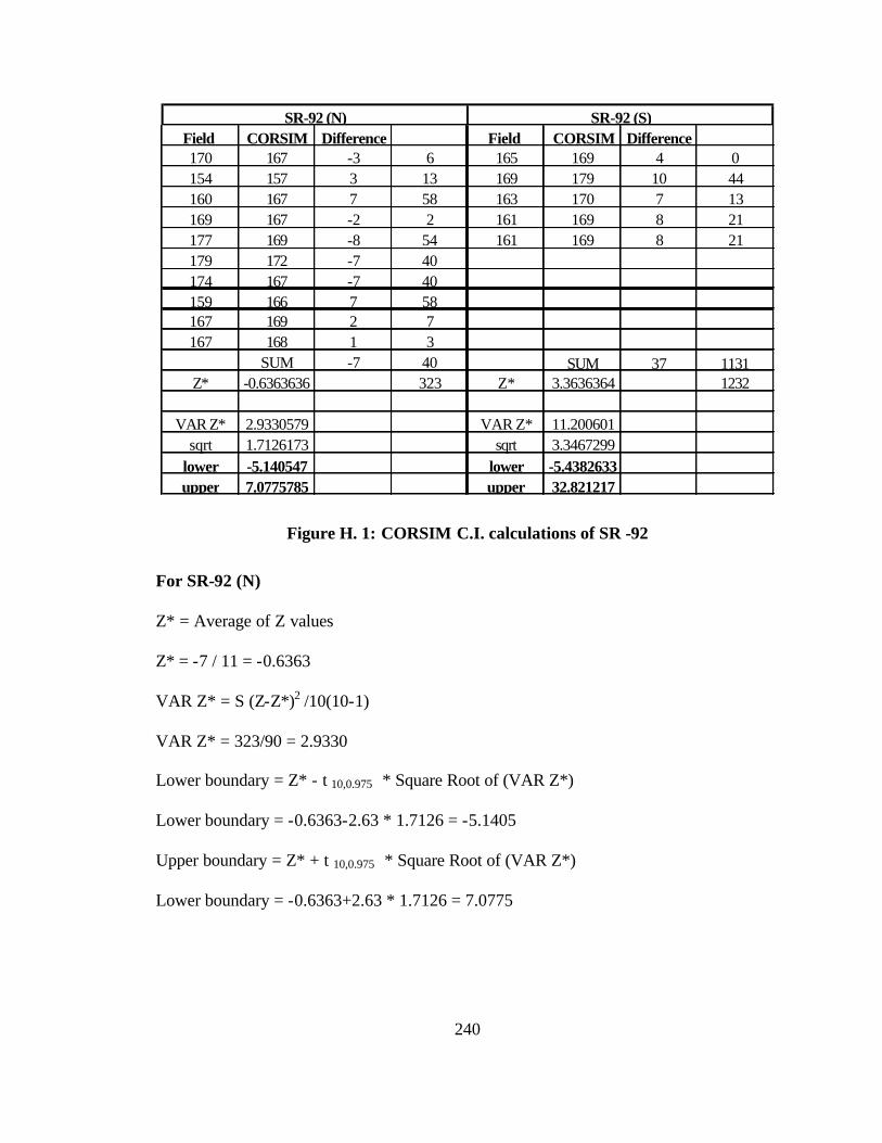
240
Field CORSIM Difference Field CORSIM Difference170 167 -3 6 165 169 4 0154 157 3 13 169 179 10 44160 167 7 58 163 170 7 13169 167 -2 2 161 169 8 21177 169 -8 54 161 169 8 21179 172 -7 40174 167 -7 40159 166 7 58167 169 2 7167 168 1 3
SUM -7 40 SUM 37 1131Z* -0.6363636 323 Z* 3.3636364 1232
VAR Z* 2.9330579 VAR Z* 11.200601sqrt 1.7126173 sqrt 3.3467299
lower -5.140547 lower -5.4382633upper 7.0775785 upper 32.821217
SR-92 (N) SR-92 (S)
Figure H. 1: CORSIM C.I. calculations of SR -92
For SR-92 (N)
Z* = Average of Z values
Z* = -7 / 11 = -0.6363
VAR Z* = S (Z-Z*)2 /10(10-1)
VAR Z* = 323/90 = 2.9330
Lower boundary = Z* - t 10,0.975 * Square Root of (VAR Z*)
Lower boundary = -0.6363-2.63 * 1.7126 = -5.1405
Upper boundary = Z* + t 10,0.975 * Square Root of (VAR Z*)
Lower boundary = -0.6363+2.63 * 1.7126 = 7.0775
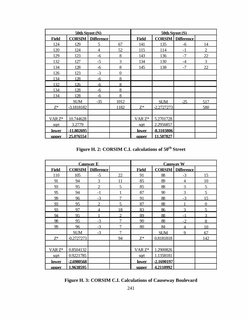
241
Field CORSIM Difference Field CORSIM Difference124 129 5 67 141 135 -6 14120 124 4 52 115 114 -1 2129 123 -6 8 143 136 -7 22132 127 -5 3 134 130 -4 3134 128 -6 8 145 138 -7 22126 123 -3 0134 128 -6 8132 126 -6 8134 128 -6 8134 128 -6 8
SUM -35 1012 SUM -25 517Z* -3.1818182 1182 Z* -2.2727273 580
VAR Z* 10.744628 VAR Z* 5.2701728sqrt 3.2779 sqrt 2.2956857
lower -11.802695 lower -8.3103806upper 25.076554 upper 11.587827
50th Street (N) 50th Street (S)
Figure H. 2: CORSIM C.I. calculations of 50th Street
Field CORSIM Difference Field CORSIM Difference110 105 -5 22 91 88 -3 1591 94 3 11 85 89 4 1093 95 2 5 85 88 3 595 94 -1 1 87 90 3 599 96 -3 7 91 88 -3 1593 95 2 5 87 88 1 093 97 4 18 83 86 3 594 95 1 2 89 88 -1 398 95 -3 7 90 88 -2 899 96 -3 7 80 84 4 10
SUM -3 7 SUM 9 67Z* -0.2727273 94 Z* 0.8181818 142
VAR Z* 0.8504132 VAR Z* 1.2900826sqrt 0.9221785 sqrt 1.1358181
lower -2.6980568 lower -2.1690197upper 1.9638595 upper 4.2110992
Causway E Causway W
Figure H. 3: CORSIM C.I. Calculations of Causeway Boulevard

242
Field CORSIM Difference Field CORSIM Difference158 155 -3 9 117 124 7 107159 156 -3 9 118 113 -5 3154 155 1 1 115 110 -5 3150 155 5 25 119 114 -5 3142 148 6 36 120 115 -5 3156 155 -1 1 112 108 -4 0158 156 -2 4 113 108 -5 3153 155 2 4 114 109 -5 3159 154 -5 25 114 109 -5 3
SUM 0 0 120 115 -5 3Z* 0 114 SUM -37 1131
Z* -3.3636364 1261VAR Z* 1.0363636
sqrt 1.0180195 VAR Z* 11.460331lower -2.6773912 sqrt 3.385311upper 2.7256364 lower -12.267004
upper 26.777033
22nd ST 21st ST
Figure H. 4: CORSIM C.I. Calculations of 22nd and 21st Streets

243
APPENDIX I VISSIM Calibration Tables Using FDOT Data

244
1 3 4 5 6 7 8 9 10 11 12 13 14 16 18
1 0 100 250 0 25 100 0 600 0 0 0 0 0 0 150
3 100 0 500 0 0 0 500 250 0 0 0 0 0 0 04 0 500 0 0 0 0 0 0 0 0 0 0 0 0 200
5 0 0 0 0 0 0 0 0 0 0 0 0 0 0 150
6 40 0 0 0 0 0 0 250 100 0 400 0 0 350 07 0 0 0 0 0 0 0 500 150 0 1300 0 0 0 50
8 0 0 0 0 0 0 0 0 0 0 0 0 0 350 09 700 0 350 0 850 50 0 0 0 0 1000 0 50 150 0
10 50 0 0 0 500 150 0 0 0 0 0 100 100 300 0
11 0 0 0 0 0 0 0 0 0 0 300 0 0 250 012 0 0 0 0 300 500 0 100 0 150 0 0 450 0 0
13 0 0 0 0 0 0 0 0 50 0 0 0 0 120 0
14 0 0 0 0 0 0 0 500 200 400 0 0 200 016 0 0 0 0 0 0 100 100 250 200 50 100 350 0 0
18 350 100 250 100 0 50 50 150 0 0 0 0 0 0 0
Figure I. 1: O-D Matrix of the 13th iteration
FDOT Data Simulated Data % error FDOT Data Simulated Data % errorL-14 570 550 3.70 488 664 26.58L-20 493 546 9.80 578 593 2.53L-23 928 840 10.42 1089 1219 10.63L-24 1011 686 47.39 861 710 21.27L-25 830 755 9.88 573 691 17.15L-30 983 717 37.03 856 804 6.41
Link Number
Inbound Outbound
Table I. 1: FDOT and VISSIM Simulated Volumes for the Master Links (13th Iteration)
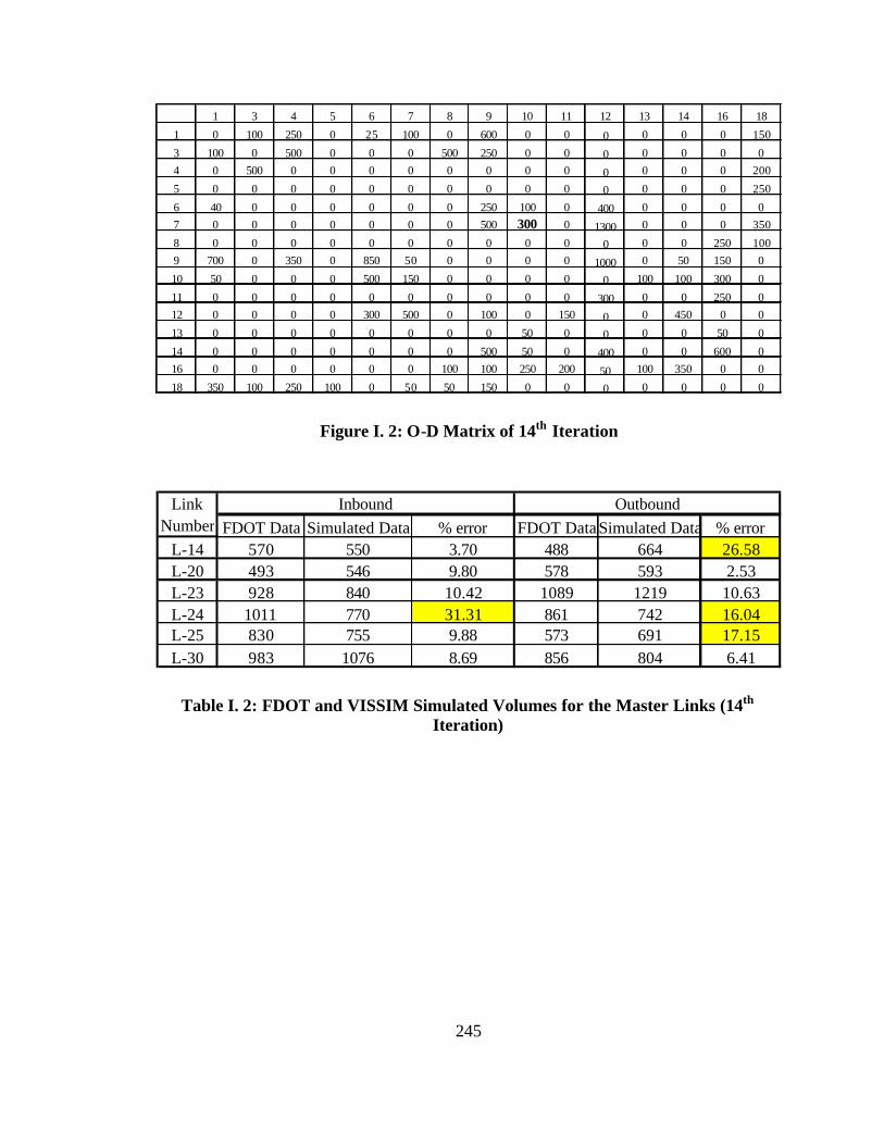
245
1 3 4 5 6 7 8 9 10 11 12 13 14 16 18
1 0 100 250 0 25 100 0 600 0 0 0 0 0 0 150
3 100 0 500 0 0 0 500 250 0 0 0 0 0 0 04 0 500 0 0 0 0 0 0 0 0 0 0 0 0 200
5 0 0 0 0 0 0 0 0 0 0 0 0 0 0 250
6 40 0 0 0 0 0 0 250 100 0 400 0 0 0 07 0 0 0 0 0 0 0 500 300 0 1300 0 0 0 350
8 0 0 0 0 0 0 0 0 0 0 0 0 0 250 1009 700 0 350 0 850 50 0 0 0 0 1000 0 50 150 0
10 50 0 0 0 500 150 0 0 0 0 0 100 100 300 0
11 0 0 0 0 0 0 0 0 0 0 300 0 0 250 012 0 0 0 0 300 500 0 100 0 150 0 0 450 0 0
13 0 0 0 0 0 0 0 0 50 0 0 0 0 50 0
14 0 0 0 0 0 0 0 500 50 0 400 0 0 600 016 0 0 0 0 0 0 100 100 250 200 50 100 350 0 0
18 350 100 250 100 0 50 50 150 0 0 0 0 0 0 0
Figure I. 2: O-D Matrix of 14th Iteration
FDOT Data Simulated Data % error FDOT Data Simulated Data % errorL-14 570 550 3.70 488 664 26.58L-20 493 546 9.80 578 593 2.53L-23 928 840 10.42 1089 1219 10.63L-24 1011 770 31.31 861 742 16.04L-25 830 755 9.88 573 691 17.15L-30 983 1076 8.69 856 804 6.41
Link Number
Inbound Outbound
Table I. 2: FDOT and VISSIM Simulated Volumes for the Master Links (14th Iteration)

246
1 3 4 5 6 7 8 9 10 11 12 13 14 16 18
1 0 100 250 0 25 100 0 600 0 0 0 0 0 0 150
3 100 0 500 0 0 0 500 250 0 0 0 0 0 0 04 0 500 0 0 0 0 0 0 0 0 0 0 0 0 200
5 0 0 0 0 0 0 0 0 100 0 0 0 0 0 250
6 40 0 0 0 0 0 0 250 100 0 400 0 0 0 07 0 0 0 0 0 0 0 500 450 0 1300 0 0 0 350
8 0 0 0 0 0 0 0 0 0 0 0 0 0 250 1009 700 0 350 0 850 50 0 0 0 0 1000 0 50 150 0
10 50 0 0 0 500 150 0 0 0 0 0 100 100 300 0
11 0 0 0 0 0 0 0 0 0 0 300 0 0 250 012 0 0 0 0 300 500 0 100 0 150 0 0 450 0 0
13 0 0 0 0 0 0 0 0 50 0 0 0 0 50 0
14 0 0 0 0 0 0 0 500 50 0 400 0 0 600 016 0 0 0 0 0 0 100 100 250 200 50 100 350 0 0
18 350 100 250 100 0 50 50 150 0 0 0 0 0 0 0
Figure I. 3: O-D Matrix of 15th Iteration
FDOT Data Simulated Data % error FDOT Data Simulated Data % errorL-14 570 550 3.70 488 664 26.58L-20 493 546 9.80 578 593 2.53L-23 928 840 10.42 1089 1219 10.63L-24 1011 940 7.56 861 742 16.04L-25 830 755 9.88 573 691 17.15L-30 983 1076 8.69 856 804 6.41
Inbound Outbound
Table I. 3: FDOT and VISSIM Simulated Volumes for the Master Links (15th Iteration)

247
1 3 4 5 6 7 8 9 10 11 12 13 14 16 18
1 0 100 250 0 25 100 0 600 0 0 0 0 0 0 1503 100 0 500 0 0 0 500 250 0 0 0 0 0 0 0
4 0 500 0 0 0 0 0 0 0 0 0 0 0 0 200
5 0 0 0 0 0 0 0 0 100 0 0 0 0 0 2506 40 0 0 0 0 0 0 250 100 0 400 0 0 0 0
7 0 0 0 0 0 0 0 500 450 0 1300 0 0 0 350
8 0 0 0 0 0 0 0 0 0 0 0 0 0 250 1009 700 0 350 0 850 50 0 0 0 0 1000 0 50 150 0
10 50 0 0 0 500 150 0 0 0 0 0 100 100 300 0
11 0 0 0 0 0 0 0 0 0 0 300 0 0 250 012 0 0 0 0 300 500 0 100 0 150 0 0 450 0 0
13 0 0 0 0 0 0 0 0 50 0 0 0 0 50 014 0 0 0 0 0 0 0 500 200 0 400 0 0 250 0
16 0 0 0 0 0 0 120 120 300 240 50 120 200 0 0
18 350 100 250 100 0 50 50 150 0 0 0 0 0 0 0
Figure I. 4: O-D Matrix of the 16th Iteration
FDOT Data Simulated Data % error FDOT Data Simulated Data % errorL-14 570 550 3.70 488 558 12.63L-20 493 546 9.80 578 593 2.53L-23 928 840 10.42 1089 1219 10.63L-24 1011 940 7.56 861 809 6.43L-25 830 755 9.88 573 653 15.93L-30 983 1076 8.69 856 930 8.01
Inbound Outbound
Table I. 4: FDOT and VISSIM Simulated Volumes for the Master Links (16th Iteration)

248
1 3 4 5 6 7 8 9 10 11 12 13 14 16 18
1 0 100 250 0 25 100 0 600 0 0 0 0 0 0 1503 100 0 500 0 0 0 500 250 0 0 0 0 0 0 0
4 0 500 0 0 0 0 0 0 0 0 0 0 0 0 200
5 0 0 0 0 0 0 0 0 100 0 0 0 0 0 2506 40 0 0 0 0 0 0 250 450 0 400 0 0 0 0
7 0 0 0 0 0 0 0 500 0 0 1300 0 0 0 350
8 0 0 0 0 0 0 0 0 0 0 0 0 0 290 1009 700 350 0 0 850 50 0 0 0 0 1000 0 50 175 0
10 50 0 0 0 500 150 0 0 0 0 0 100 100 150 0
11 0 0 0 0 0 0 0 0 0 0 300 0 0 290 012 0 0 0 0 300 500 0 100 0 150 0 0 450 0 0
13 0 0 0 0 0 0 0 0 50 0 0 0 0 58 014 0 0 0 0 0 0 0 500 200 0 400 0 0 290 0
16 0 0 0 0 0 0 120 120 300 240 50 120 200 0 0
18 350 100 250 100 0 50 50 150 0 0 0 0 0 0 0
Figure I. 5: O-D Matrix of the 17th Iteration
FDOT Data Simulated Data % error FDOT Data Simulated Data % errorL-14 570 550 3.70 488 558 12.63L-20 493 546 9.80 578 593 2.53L-23 928 840 10.42 1089 1219 10.63L-24 1011 940 7.56 861 809 6.43
L-25 830 755 9.88 573 615 6.91L-30 983 1076 8.69 856 930 8.01
Inbound Outbound
Table I. 5: FDOT and CORSIM Simulated Volumes for the Master Links (17th Iteration)

249
APPENDIX J Final Calibration Tables for VISSIM Field Calibrated O-D Matrices
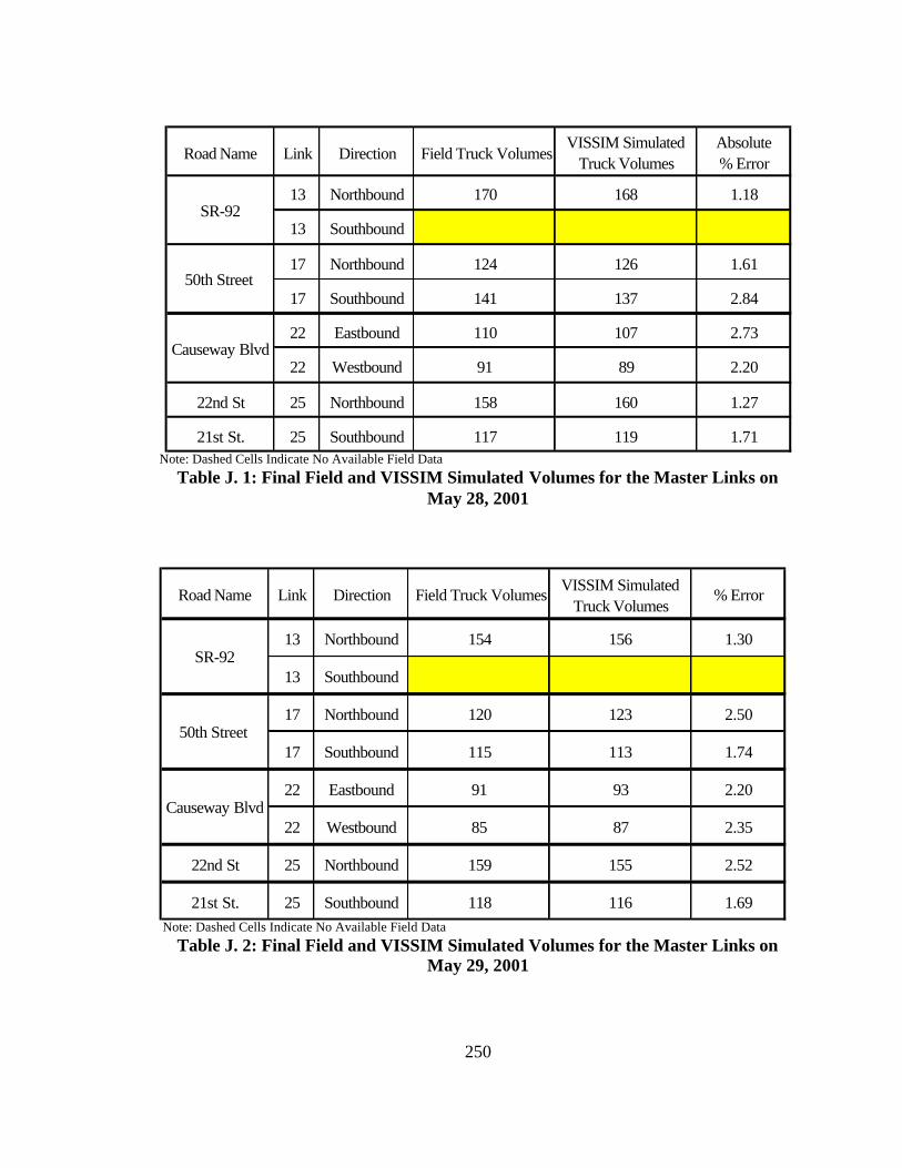
250
Road Name Link Direction Field Truck VolumesVISSIM Simulated
Truck VolumesAbsolute % Error
13 Northbound 170 168 1.18
13 Southbound
17 Northbound 124 126 1.61
17 Southbound 141 137 2.84
22 Eastbound 110 107 2.73
22 Westbound 91 89 2.20
22nd St 25 Northbound 158 160 1.27
21st St. 25 Southbound 117 119 1.71
SR-92
50th Street
Causeway Blvd
Note: Dashed Cells Indicate No Available Field Data
Table J. 1: Final Field and VISSIM Simulated Volumes for the Master Links on May 28, 2001
Road Name Link Direction Field Truck Volumes VISSIM Simulated Truck Volumes
% Error
13 Northbound 154 156 1.30
13 Southbound
17 Northbound 120 123 2.50
17 Southbound 115 113 1.74
22 Eastbound 91 93 2.20
22 Westbound 85 87 2.35
22nd St 25 Northbound 159 155 2.52
21st St. 25 Southbound 118 116 1.69
50th Street
Causeway Blvd
SR-92
Note: Dashed Cells Indicate No Available Field Data
Table J. 2: Final Field and VISSIM Simulated Volumes for the Master Links on May 29, 2001

251
Road Name Link Direction Field Truck Volumes VISSIM Simulated Truck Volumes
% Error
13 Northbound 160 165 3.13
13 Southbound
17 Northbound 129 131 1.55
17 Southbound 143 138 3.50
22 Eastbound 93 94 1.08
22 Westbound 85 86 1.18
22nd St 25 Northbound 154 155 0.65
21st St. 25 Southbound 115 112 2.61
Causeway Blvd
SR-92
50th Street
Note: Dashed Cells Indicate No Available Field Data
Table J. 3: Final Field and VISSIM Simulated Volumes for the Master Links on May 30, 2001
Road Name Link Direction Field Truck VolumesVISSIM Simulated
Truck Volumes% Error
13 Northbound 169 166 1.78
13 Southbound
17 Northbound 132 130 1.52
17 Southbound 134 131 2.24
22 Eastbound 95 96 1.05
22 Westbound 87 89 2.30
22nd St 25 Northbound 150 154 2.67
21st St. 25 Southbound 119 115 3.36
SR-92
50th Street
Causeway Blvd
Note: Dashed Cells Indicate No Available Field Data
Table J. 4: Final Field and VISSIM Simulated Volumes for the Master Links on May 31, 2001
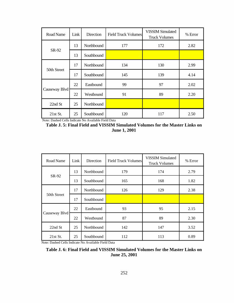
252
Road Name Link Direction Field Truck VolumesVISSIM Simulated
Truck Volumes% Error
13 Northbound 177 172 2.82
13 Southbound
17 Northbound 134 130 2.99
17 Southbound 145 139 4.14
22 Eastbound 99 97 2.02
22 Westbound 91 89 2.20
22nd St 25 Northbound
21st St. 25 Southbound 120 117 2.50
SR-92
50th Street
Causeway Blvd
Note: Dashed Cells Indicate No Available Field Data
Table J. 5: Final Field and VISSIM Simulated Volumes for the Master Links on June 1, 2001
Note: Dashed Cells Indicate No Available Field Data
Table J. 6: Final Field and VISSIM Simulated Volumes for the Master Links on June 25, 2001
Road Name Link Direction Field Truck VolumesVISSIM Simulated
Truck Volumes% Error
13 Northbound 179 174 2.79
13 Southbound 165 168 1.82
17 Northbound 126 129 2.38
17 Southbound
22 Eastbound 93 95 2.15
22 Westbound 87 89 2.30
22nd St 25 Northbound 142 147 3.52
21st St. 25 Southbound 112 113 0.89
50th Street
Causeway Blvd
SR-92

253
Road Name Link Direction Field Truck VolumesVISSIM Simulated
Truck Volumes% Error
13 Northbound 174 169 2.87
13 Southbound 169 175 3.55
17 Northbound 134 131 2.24
17 Southbound
22 Eastbound 93 95 2.15
22 Westbound 83 87 4.82
22nd St 25 Northbound 156 153 1.92
21st St. 25 Southbound 113 111 1.77
Causeway Blvd
SR-92
50th Street
Note: Dashed Cells Indicate No Available Field Data
Table J. 7: Final Field and VISSIM Simulated Volumes for the Master Links on June 26, 2001
Road Name Link Direction Field Truck VolumesVISSIM Simulated
Truck Volumes% Error
13 Northbound 159 163 2.52
13 Southbound 163 168 3.07
17 Northbound 132 128 3.03
17 Southbound
22 Eastbound 94 96 2.13
22 Westbound 89 88 1.12
22nd St 25 Northbound 158 157 0.63
21st St. 25 Southbound 114 117 2.63
SR-92
50th Street
Causeway Blvd
Note: Dashed Cells Indicate No Available Field Data
Table J. 8: Final Field and VISSIM Simulated Volumes for the Master Links on June 27, 2001

254
Road Name Link Direction Field Truck VolumesVISSIM Simulated
Truck Volumes% Error
13 Northbound 167 170 1.80
13 Southbound 161 165 2.48
17 Northbound 134 136 1.49
17 Southbound
22 Eastbound 98 97 1.02
22 Westbound 90 87 3.33
22nd St 25 Northbound 153 155 1.31
21st St. 25 Southbound 114 118 3.51
SR-92
50th Street
Causeway Blvd
Note: Dashed Cells Indicate No Available Field Data
Table J. 9: Final Field and VISSIM Simulated Volumes for the Master Links on June 28, 2001
Road Name Link Direction Field Truck VolumesVISSIM Simulated
Truck Volumes% Error
13 Northbound 167 168 0.60
13 Southbound 161 166 3.11
17 Northbound 134 130 2.99
17 Southbound
22 Eastbound 99 97 2.02
22 Westbound 80 83 3.75
22nd St 25 Northbound 159 155 2.52
21st St. 25 Southbound 120 117 2.50
50th Street
Causeway Blvd
SR-92
Note: Dashed Cells Indicate No Available Field Data
Table J. 10: Final Field and VISSIM Simulated Volumes for the Master Links on June 29, 2001

255
APPENDIX K C.I. Method for VISSIM Model Calibration

256
Field VISSIM Difference (Z) (Z-Z*)2 Field VISSIM Difference (Z) (Z-Z*)2208 212 3 20 242 243 1 1234 209 -25 556 211 225 15 165222 217 -5 16 233 239 6 15223 220 -3 5 253 246 -7 77217 226 9 100 227 235 7 30230 234 4 27 220 211 -9 112219 217 -2 1 231 237 6 16216 214 -3 2 228 231 3 2214 212 -2 1 241 240 -1 10242 244 3 15 230 234 4 6230 238 8 85 221 216 -5 46
SUM -13 148 SUM 22 386Z* -1.21818182 975 Z* 1.963636 864
VAR Z* 8.86284598 VAR Z* 7.851384sqrt 2.977053238 sqrt 2.802032
lower -9.04783183 lower -5.40571upper 6.611468197 upper 9.332981
SR-92 (N) SR-92 (S)
Figure K. 1: VISSIM C.I. calculations of SR -92
Field VISSIM Difference (Z) (Z-Z*)2 Field VISSIM Difference (Z) (Z-Z*)2168 182 14 130 161 165 4 80168 181 13 112 154 155 1 35153 149 -3 32 153 148 -5 0154 153 -1 12 191 170 -21 264147 146 -2 16 175 168 -7 5182 186 3 1 173 159 -14 86186 187 1 1 170 177 7 143188 192 4 2 171 164 -7 5174 170 -5 52 161 158 -4 1150 153 3 0 167 164 -3 2155 154 -1 10 161 157 -4 1
SUM 27 585 SUM -50 2066Z* 2.418181818 952 Z* -4.54545 2688
VAR Z* 8.658879038 VAR Z* 24.44039sqrt 2.942597329 sqrt 4.943722
lower -5.32084916 lower -17.5474upper 10.15721279 upper 8.456535
50th Street (S)50th Street (N)
Figure K. 2: VISSIM C.I. calculations of 50th Street

257
Field VISSIM Difference (Z) (Z-Z*)2 Field VISSIM Difference (Z) (Z-Z*)2140 124 -16 106 130 112 -18 353127 116 -11 26 124 123 -1 3130 122 -8 6 120 120 0 1124 118 -6 0 124 123 -1 3124 121 -3 6 136 137 1 0148 148 0 26 124 136 12 139119 112 -7 4 118 125 7 38101 107 6 137 108 113 5 23122 118 -4 1 91 93 2 1121 118 -2 11 125 126 1 0124 115 -9 12 123 122 -1 3
SUM -60 3015 SUM 7 36Z* -5.49090909 3351 Z* 0.6 602
VAR Z* 30.45961232 VAR Z* 5.474182sqrt 5.519022769 sqrt 2.339697
lower -20.005939 lower -5.5534upper 9.024120791 upper 6.753403
Causway E Causway W
Figure K. 3: VISSIM C.I. Calculations of Causeway Boulevard
Field VISSIM Difference (Z) (Z-Z*)2 Field VISSIM Difference (Z) (Z-Z*)2184 179 -5 1 127 130 3 7196 192 -4 6 137 135 -1 2184 176 -8 4 142 137 -5 29182 179 -3 14 123 125 2 3164 167 3 91 120 132 11 130197 182 -14 61 126 126 1 0192 174 -18 145 150 154 4 16186 178 -8 3 133 128 -5 25184 178 -6 1 157 156 -1 2178 181 3 84 136 127 -9 74198 189 -9 9 121 123 2 3
SUM -70 4050 SUM 0 0Z* -6.36363636 4470 Z* 1.29E-15 290
VAR Z* 40.63392938 VAR Z* 2.638545sqrt 6.374474831 sqrt 1.62436
lower -23.1285052 lower -4.27207upper 10.40123244 upper 4.272067
22nd St. 21st St
Figure K. 4: VISSIM C.I. Calculations of 22nd and 21st Streets

258
APPENDIX L Validation O-D Matrices for CORSIM and VISSIM

259
1 (Port) 1 south 3 4 5 6 7 8 9 10 11 12 13 14 16 (Port) 18 (Port) Sum.
1 (Port) 0 0 30 0 0 10 0 0 0 0 0 0 0 0 0 0 40
1 south 0 0 0 50 0 0 20 0 53 10 0 0 0 0 0 26
3 20 0 0 100 0 0 0 100 0 0 0 0 0 0 0 0
4 0 0 100 0 0 0 0 0 32 0 0 0 0 0 0 42
5 16 0 0 0 0 0 0 0 0 0 0 0 0 0 0 27
6 8 0 0 0 0 0 0 0 51 60 0 78 0 0 0 0
7 0 0 0 0 0 0 0 0 26 152 0 260 0 0 0 15
8 0 0 76 0 0 0 0 0 0 0 0 0 0 0 0 0
9 0 143 0 4 0 150 10 0 0 0 0 200 0 10 24 0
10 0 15 0 0 0 100 30 0 0 0 0 0 40 30 10 0
11 0 0 0 0 0 0 0 0 0 0 0 60 0 0 44 0
12 0 0 0 0 0 80 120 0 20 0 60 0 0 216 10 0
13 0 0 0 0 0 0 0 0 0 10 0 0 0 0 24 0
14 0 0 0 0 0 0 0 0 30 40 0 79 0 0 40 0
16 (Port) 0 0 0 0 0 0 0 4 22 44 88 10 10 20 0 0 198
18 (Port) 0 60 10 40 10 0 8 8 0 0 0 0 0 0 0 0 136
Sum. 44 152 110
Destination Nodes
Ori
gin
Nod
es
Figure L. 1: The Truck O-D Matrix for the Peak Hour on 5th of July 2001
1 (Port) 1 south 3 4 5 6 7 8 9 10 11 12 13 14 16 (Port) 18 (Port) Sum.
1 (Port) 0 0 33 0 0 10 0 0 0 0 0 0 0 0 0 0 43
1 south 0 0 0 50 0 0 20 0 53 10 0 0 0 0 0 25
3 19 0 0 100 0 0 0 100 0 0 0 0 0 0 0 0
4 0 0 100 0 0 0 0 0 32 0 0 0 0 0 0 40
5 15 0 0 0 0 0 0 0 0 0 0 0 0 0 0 25
6 6 0 0 0 0 0 0 0 51 60 0 78 0 0 0 0
7 0 0 0 0 0 0 0 0 26 152 0 260 0 0 0 15
8 0 0 76 0 0 0 0 0 0 0 0 0 0 0 0 0
9 0 143 0 4 0 150 10 0 0 0 0 200 0 10 24 0
10 0 15 0 0 0 100 30 0 0 0 0 0 40 30 10 0
11 0 0 0 0 0 0 0 0 0 0 0 60 0 0 44 0
12 0 0 0 0 0 80 120 0 20 0 60 0 0 216 10 0
13 0 0 0 0 0 0 0 0 0 10 0 0 0 0 24 0
14 0 0 0 0 0 0 0 0 30 40 0 79 0 0 40 0
16 (Port) 0 0 0 0 0 0 0 4 22 44 88 10 10 20 0 0 198
18 (Port) 0 60 10 40 10 0 8 8 0 0 0 0 0 0 0 0 136
Sum. 40 152 105
Destination Nodes
Ori
gin
Nod
es
Figure L. 2: The Truck O-D Matrix for the Peak Hour on 6th of July 2001

260
1 (Port) 1 south 3 4 5 6 7 8 9 10 11 12 13 14 16 (Port) 18 (Port) Sum.
1 (Port) 0 0 30 0 0 9 0 0 0 0 0 0 0 0 0 0 39
1 south 0 0 0 50 0 0 20 0 53 10 0 0 0 0 0 25
3 19 0 0 100 0 0 0 100 0 0 0 0 0 0 0 0
4 0 0 100 0 0 0 0 0 32 0 0 0 0 0 0 40
5 16 0 0 0 0 0 0 0 0 0 0 0 0 0 0 25
6 6 0 0 0 0 0 0 0 51 60 0 78 0 0 0 0
7 0 0 0 0 0 0 0 0 26 152 0 260 0 0 0 11
8 0 0 76 0 0 0 0 0 0 0 0 0 0 0 0 0
9 0 143 0 4 0 150 10 0 0 0 0 200 0 10 24 0
10 0 15 0 0 0 100 30 0 0 0 0 0 40 30 10 0
11 0 0 0 0 0 0 0 0 0 0 0 60 0 0 40 0
12 0 0 0 0 0 80 120 0 20 0 60 0 0 216 10 0
13 0 0 0 0 0 0 0 0 0 10 0 0 0 0 20 0
14 0 0 0 0 0 0 0 0 30 40 0 79 0 0 35 0
16 (Port) 0 0 0 0 0 0 0 5 17 44 90 10 10 20 0 0 196
18 (Port) 0 59 10 40 10 0 8 8 0 0 0 0 0 0 0 0 135
Sum. 41 139 101
Destination Nodes
Ori
gin
Nod
es
Figure L. 3: The Truck O-D Matrix for the Peak Hour on 9th of July 2001
1 (Port) 1 south 3 4 5 6 7 8 9 10 11 12 13 14 16 (Port) 18 (Port) Sum.
1 (Port) 0 0 30 0 0 10 0 0 0 0 0 0 0 0 0 0 40
1 south 0 0 0 50 0 0 20 0 53 10 0 0 0 0 0 24
3 17 0 0 100 0 0 0 100 0 0 0 0 0 0 0 0
4 0 0 100 0 0 0 0 0 32 0 0 0 0 0 0 39
5 14 0 0 0 0 0 0 0 0 0 0 0 0 0 0 25
6 8 0 0 0 0 0 0 0 51 60 0 78 0 0 0 0
7 0 0 0 0 0 0 0 0 26 152 0 260 0 0 0 10
8 0 0 76 0 0 0 0 0 0 0 0 0 0 0 0 0
9 0 143 0 4 0 150 10 0 0 0 0 200 0 10 21 0
10 0 15 0 0 0 100 30 0 0 0 0 0 40 30 10 0
11 0 0 0 0 0 0 0 0 0 0 0 60 0 0 40 0
12 0 0 0 0 0 80 120 0 20 0 60 0 0 216 10 0
13 0 0 0 0 0 0 0 0 0 10 0 0 0 0 20 0
14 0 0 0 0 0 0 0 0 30 40 0 79 0 0 34 0
16 (Port) 0 0 0 0 0 0 0 6 17 44 90 10 10 18 0 0 195
18 (Port) 0 59 10 39 10 0 8 8 0 0 0 0 0 0 0 0 134
Sum. 39 135 98
Destination Nodes
Ori
gin
Nod
es
Figure L. 4: The Truck O-D Matrix for the Peak Hour on 10th of July 2001

261
1 (Port) 1 south 3 4 5 6 7 8 9 10 11 12 13 14 16 (Port) 18 (Port) Sum.
1 (Port) 0 0 30 0 0 10 0 0 0 0 0 0 0 0 0 0 40
1 south 0 0 0 50 0 0 20 0 53 10 0 0 0 0 0 24
3 19 0 0 100 0 0 0 100 0 0 0 0 0 0 0 0
4 0 0 100 0 0 0 0 0 32 0 0 0 0 0 0 40
5 15 0 0 0 0 0 0 0 0 0 0 0 0 0 0 25
6 8 0 0 0 0 0 0 0 51 60 0 78 0 0 0 0
7 0 0 0 0 0 0 0 0 26 152 0 260 0 0 0 10
8 0 0 76 0 0 0 0 0 0 0 0 0 0 0 0 0
9 0 143 0 4 0 150 10 0 0 0 0 200 0 10 26 0
10 0 15 0 0 0 100 30 0 0 0 0 0 40 30 10 0
11 0 0 0 0 0 0 0 0 0 0 0 60 0 0 42 0
12 0 0 0 0 0 80 120 0 20 0 60 0 0 216 10 0
13 0 0 0 0 0 0 0 0 0 10 0 0 0 0 20 0
14 0 0 0 0 0 0 0 0 30 40 0 79 0 0 35 0
16 (Port) 0 0 0 0 0 0 0 6 18 45 90 10 10 18 0 0 197
18 (Port) 0 60 10 39 10 0 8 8 0 0 0 0 0 0 0 0 135
Sum. 42 143 99
Destination Nodes
Ori
gin
Nod
es
Figure L. 5: The Truck O-D Matrix for the Peak Hour on 16th of July 2001
1 (Port) 1 south 3 4 5 6 7 8 9 10 11 12 13 14 16 (Port) 18 (Port) Sum.
1 (Port) 0 0 30 0 0 9 0 0 0 0 0 0 0 0 0 0 39
1 south 0 0 0 50 0 0 20 0 53 10 0 0 0 0 0 24
3 19 0 0 100 0 0 0 100 0 0 0 0 0 0 0 0
4 0 0 100 0 0 0 0 0 32 0 0 0 0 0 0 40
5 15 0 0 0 0 0 0 0 0 0 0 0 0 0 0 25
6 6 0 0 0 0 0 0 0 51 60 0 78 0 0 0 0
7 0 0 0 0 0 0 0 0 26 152 0 260 0 0 0 10
8 0 0 76 0 0 0 0 0 0 0 0 0 0 0 0 0
9 0 143 0 4 0 150 10 0 0 0 0 200 0 10 21 0
10 0 15 0 0 0 100 30 0 0 0 0 0 40 30 8 0
11 0 0 0 0 0 0 0 0 0 0 0 60 0 0 39 0
12 0 0 0 0 0 80 120 0 20 0 60 0 0 216 8 0
13 0 0 0 0 0 0 0 0 0 10 0 0 0 0 22 0
14 0 0 0 0 0 0 0 0 30 40 0 79 0 0 38 0
16 (Port) 0 0 0 0 0 0 0 5 17 44 90 10 10 20 0 0 196
18 (Port) 0 58 10 40 10 0 8 8 0 0 0 0 0 0 0 0 134
Sum. 40 136 99
Destination Nodes
Ori
gin
Nod
es
Figure L. 6: The Truck O-D Matrix for the Peak Hour on 17th of July 2001

262
1 (Port) 1 south 3 4 5 6 7 8 9 10 11 12 13 14 16 (Port) 18 (Port) Sum.
1 (Port) 0 0 30 0 0 9 0 0 0 0 0 0 0 0 0 0 39
1 south 17 0 0 50 0 0 20 0 53 10 0 0 0 0 0 24
3 0 0 0 100 0 0 0 100 0 0 0 0 0 0 0 0
4 14 0 100 0 0 0 0 0 32 0 0 0 0 0 0 38
5 8 0 0 0 0 0 0 0 0 0 0 0 0 0 0 25
6 0 0 0 0 0 0 0 0 51 60 0 78 0 0 0 0
7 0 0 0 0 0 0 0 0 26 152 0 260 0 0 0 10
8 0 0 76 0 0 0 0 0 0 0 0 0 0 0 0 0
9 0 143 0 4 0 150 10 0 0 0 0 200 0 10 20 0
10 0 15 0 0 0 100 30 0 0 0 0 0 40 30 10 0
11 0 0 0 0 0 0 0 0 0 0 0 60 0 0 40 0
12 0 0 0 0 0 80 120 0 20 0 60 0 0 216 10 0
13 0 0 0 0 0 0 0 0 0 10 0 0 0 0 20 0
14 0 0 0 0 0 0 0 0 30 40 0 79 0 0 33 0
16 (Port) 0 0 0 0 0 0 0 5 17 44 90 10 10 20 0 0 196
18 (Port) 0 58 10 40 10 0 8 8 0 0 0 0 0 0 0 0 134
Sum. 39 133 97
Destination Nodes
Ori
gin
Nod
es
Figure L. 7: The Truck O-D Matrix for the Peak Hour on 18th of July 2001
1 (Port) 1 south 3 4 5 6 7 8 9 10 11 12 13 14 16 (Port) 18 (Port) Sum.
1 (Port) 0 0 30 0 0 10 0 0 0 0 0 0 0 0 0 0 40
1 south 0 0 0 50 0 0 20 0 53 10 0 0 0 0 0 24
3 19 0 0 100 0 0 0 100 0 0 0 0 0 0 0 0
4 0 0 100 0 0 0 0 0 32 0 0 0 0 0 0 39
5 15 0 0 0 0 0 0 0 0 0 0 0 0 0 0 25
6 6 0 0 0 0 0 0 0 51 60 0 78 0 0 0 0
7 0 0 0 0 0 0 0 0 26 152 0 260 0 0 0 10
8 0 0 76 0 0 0 0 0 0 0 0 0 0 0 0 0
9 0 143 0 4 0 150 10 0 0 0 0 200 0 10 21 0
10 0 15 0 0 0 100 30 0 0 0 0 0 40 30 10 0
11 0 0 0 0 0 0 0 0 0 0 0 60 0 0 40 0
12 0 0 0 0 0 80 120 0 20 0 60 0 0 216 10 0
13 0 0 0 0 0 0 0 0 0 10 0 0 0 0 20 0
14 0 0 0 0 0 0 0 0 30 40 0 79 0 0 34 0
16 (Port) 0 0 0 0 0 0 0 6 17 44 90 10 10 18 0 0 195
18 (Port) 0 58 10 40 10 0 8 8 0 0 0 0 0 0 0 0 134
Sum. 40 135 98
Destination Nodes
Ori
gin
Nod
es
Figure L. 8: The Truck O-D Matrix for the Peak Hour on 19th of July 2001

263
1 (Port) 1 south 3 4 5 6 7 8 9 10 11 12 13 14 16 (Port) 18 (Port) Sum.
1 (Port) 0 0 32 0 0 10 0 0 0 0 0 0 0 0 0 0 42
1 south 0 0 0 50 0 0 20 0 53 10 0 0 0 0 0 25
3 19 0 0 100 0 0 0 100 0 0 0 0 0 0 0 0
4 0 0 100 0 0 0 0 0 32 0 0 0 0 0 0 39
5 15 0 0 0 0 0 0 0 0 0 0 0 0 0 0 25
6 6 0 0 0 0 0 0 0 51 60 0 78 0 0 0 0
7 0 0 0 0 0 0 0 0 26 152 0 260 0 0 0 15
8 0 0 76 0 0 0 0 0 0 0 0 0 0 0 0 0
9 0 143 0 4 0 150 10 0 0 0 0 200 0 10 26 0
10 0 15 0 0 0 100 30 0 0 0 0 0 40 30 10 0
11 0 0 0 0 0 0 0 0 0 0 0 60 0 0 42 0
12 0 0 0 0 0 80 120 0 20 0 60 0 0 216 10 0
13 0 0 0 0 0 0 0 0 0 10 0 0 0 0 20 0
14 0 0 0 0 0 0 0 0 30 40 0 79 0 0 35 0
16 (Port) 0 0 0 0 0 0 0 6 18 45 90 10 10 18 0 0 197
18 (Port) 0 59 10 40 10 0 8 8 0 0 0 0 0 0 0 0 135
Sum. 40 143 104
Destination Nodes
Ori
gin
Nod
es
Figure L. 9: The Truck O-D Matrix for the Peak Hour on 20th of July 2001
1 (Port) 1 south 3 4 5 6 7 8 9 10 11 12 13 14 16 (Port) 18 (Port) Sum.
1 (Port) 0 0 28 0 0 6 0 0 0 0 0 0 0 0 0 0 34
1 south 0 0 0 50 0 0 20 0 53 10 0 0 0 0 0 25
3 19 0 0 100 0 0 0 100 0 0 0 0 0 0 0 0
4 0 0 100 0 0 0 0 0 32 0 0 0 0 0 0 40
5 16 0 0 0 0 0 0 0 0 0 0 0 0 0 0 25
6 6 0 0 0 0 0 0 0 51 60 0 78 0 0 0 0
7 0 0 0 0 0 0 0 0 26 152 0 260 0 0 0 11
8 0 0 76 0 0 0 0 0 0 0 0 0 0 0 0 0
9 0 143 0 4 0 150 10 0 0 0 0 200 0 10 24 0
10 0 15 0 0 0 100 30 0 0 0 0 0 40 30 10 0
11 0 0 0 0 0 0 0 0 0 0 0 60 0 0 40 0
12 0 0 0 0 0 80 120 0 20 0 60 0 0 216 10 0
13 0 0 0 0 0 0 0 0 0 10 0 0 0 0 20 0
14 0 0 0 0 0 0 0 0 30 40 0 79 0 0 35 0
16 (Port) 0 0 0 0 0 0 0 6 16 38 79 8 8 15 0 0 170
18 (Port) 0 53 8 32 8 0 8 8 0 0 0 0 0 0 0 0 117
Sum. 41 139 101
Destination Nodes
Ori
gin
Nod
es
Figure L. 10: The Truck O-D Matrix for the Peak Hour on 23rd of July 2001
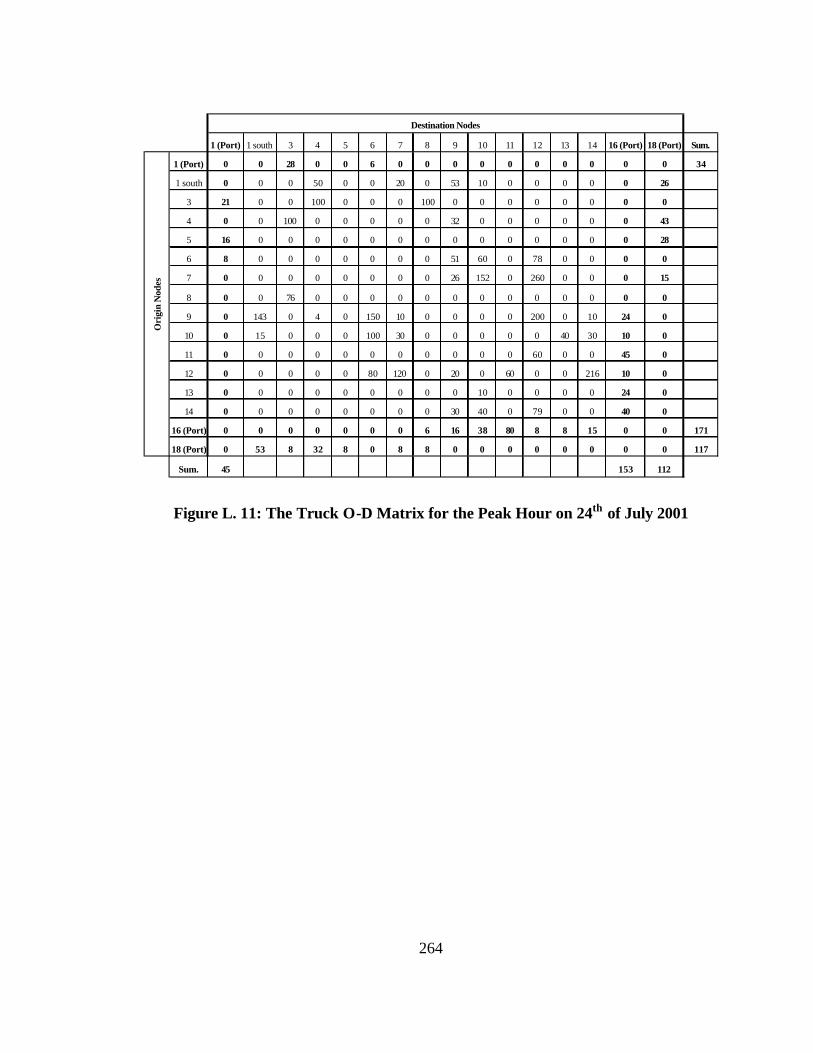
264
1 (Port) 1 south 3 4 5 6 7 8 9 10 11 12 13 14 16 (Port) 18 (Port) Sum.
1 (Port) 0 0 28 0 0 6 0 0 0 0 0 0 0 0 0 0 34
1 south 0 0 0 50 0 0 20 0 53 10 0 0 0 0 0 26
3 21 0 0 100 0 0 0 100 0 0 0 0 0 0 0 0
4 0 0 100 0 0 0 0 0 32 0 0 0 0 0 0 43
5 16 0 0 0 0 0 0 0 0 0 0 0 0 0 0 28
6 8 0 0 0 0 0 0 0 51 60 0 78 0 0 0 0
7 0 0 0 0 0 0 0 0 26 152 0 260 0 0 0 15
8 0 0 76 0 0 0 0 0 0 0 0 0 0 0 0 0
9 0 143 0 4 0 150 10 0 0 0 0 200 0 10 24 0
10 0 15 0 0 0 100 30 0 0 0 0 0 40 30 10 0
11 0 0 0 0 0 0 0 0 0 0 0 60 0 0 45 0
12 0 0 0 0 0 80 120 0 20 0 60 0 0 216 10 0
13 0 0 0 0 0 0 0 0 0 10 0 0 0 0 24 0
14 0 0 0 0 0 0 0 0 30 40 0 79 0 0 40 0
16 (Port) 0 0 0 0 0 0 0 6 16 38 80 8 8 15 0 0 171
18 (Port) 0 53 8 32 8 0 8 8 0 0 0 0 0 0 0 0 117
Sum. 45 153 112
Destination Nodes
Ori
gin
Nod
es
Figure L. 11: The Truck O-D Matrix for the Peak Hour on 24th of July 2001

265
APPENDIX M C.I. Method for CORSIM and VISSIM Models Validation

266
Field CORSIM Difference (Z) (Z-Z*)2 Field CORSIM Difference (Z) (Z-Z*)2208 220 12 179 242 237 -5 81234 222 -12 109 211 233 22 323222 220 -2 0 233 236 3 1223 219 -4 7 253 239 -13 303217 220 3 23 227 233 5 2230 224 -6 18 220 234 15 112219 220 1 8 231 234 4 0216 220 3 27 228 236 8 16214 220 6 57 241 234 -7 121242 230 -12 97 230 236 6 4230 222 -8 39 221 228 7 8
SUM -19 311 SUM 44 1615Z* -1.7636364 873 Z* 4.0181818 2586
VAR Z* 7.9395162 VAR Z* 23.511772sqrt 2.8177147 sqrt 4.8488939
lower -9.174226 lower -8.734409upper 5.6469533 upper 16.770773
SR-92 (S)SR-92 (N)
Figure M. 1: CORSIM C.I. calculations of SR -92
For SR-92 (N)
Z* = Average of Z values
Z* = -19 / 11 = -1.7636
VAR Z* = S (Z-Z*)2 /11(11-1)
VAR Z* = 873/110 = 7.9395
Lower boundary = Z* - t 10,0.975 * Square Root of (VAR Z*)
Lower boundary = -1.763-2.63 * 2.818 = -9.174
Upper boundary = Z* + t 10,0.975 * Square Root of (VAR Z*)
Lower boundary = -1.763+2.63 * 2.818 = 5.646
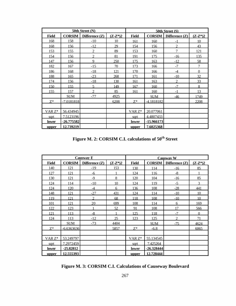
267
Field CORSIM Difference (Z) (Z-Z*)2 Field CORSIM Difference (Z) (Z-Z*)2168 158 -10 10 161 160 -1 10168 156 -12 29 154 156 2 43153 155 2 89 153 160 7 121154 156 2 81 191 175 -16 135147 156 9 250 175 163 -12 58182 167 -15 70 173 166 -7 7186 168 -18 121 170 166 -4 0188 165 -23 268 171 161 -10 32174 156 -18 130 161 163 2 33150 155 5 149 167 160 -7 8155 157 2 85 161 160 -1 13
SUM -77 4925 SUM -46 1749Z* -7.0181818 6208 Z* -4.1818182 2208
VAR Z* 56.434945 VAR Z* 20.077061sqrt 7.5123196 sqrt 4.4807433
lower -26.775582 lower -15.966173upper 12.739219 upper 7.6025368
50th Street (N) 50th Street (S)
Figure M. 2: CORSIM C.I. calculations of 50th Street
Field CORSIM Difference (Z) (Z-Z*)2 Field CORSIM Difference (Z) (Z-Z*)2140 121 -19 153 130 114 -16 85127 121 -6 1 124 116 -8 1130 121 -9 8 120 104 -16 85124 114 -10 10 124 119 -5 3124 120 -4 6 136 108 -28 441148 121 -27 431 124 114 -10 10119 121 2 68 118 108 -10 10101 121 20 699 108 114 6 169122 123 1 52 91 108 17 566121 113 -8 1 125 118 -7 0124 113 -12 25 123 125 2 71
SUM -73 4404 SUM -75 4624Z* -6.6363636 5857 Z* -6.8 6065
VAR Z* 53.249797 VAR Z* 55.134545sqrt 7.2972459 sqrt 7.425264
lower -25.82812 lower -26.328444upper 12.555393 upper 12.728444
Causway E Causway W
Figure M. 3: CORSIM C.I. Calculations of Causeway Boulevard

268
Field CORSIM Difference (Z) (Z-Z*)2 Field CORSIM Difference (Z) (Z-Z*)2184 178 -6 4 127 126 -2 18196 190 -6 4 137 132 -5 1184 178 -6 4 142 129 -13 58182 178 -4 0 123 127 4 96164 190 26 907 120 130 9 225197 179 -18 182 126 122 -4 3192 170 -22 320 150 128 -23 289186 181 -5 0 133 127 -6 0184 190 6 102 157 131 -27 433178 184 6 102 136 128 -8 6198 181 -17 171 121 132 11 269
SUM -45 1688 SUM -64 3364Z* -4.1090909 3484 Z* -5.8 4761
VAR Z* 31.675745 VAR Z* 43.279273sqrt 5.6281209 sqrt 6.5786984
lower -18.911049 lower -23.101977upper 10.692867 upper 11.501977
22nd St. 21st St
Figure M. 4: CORSIM C.I. Calculations of 22nd and 21st Streets
Field VISSIM Difference (Z) (Z-Z*)2 Field VISSIM Difference (Z) (Z-Z*)2208 212 3 20 242 243 1 1234 209 -25 556 211 225 15 165222 217 -5 16 233 239 6 15223 220 -3 5 253 246 -7 77217 226 9 100 227 235 7 30230 234 4 27 220 211 -9 112219 217 -2 1 231 237 6 16216 214 -3 2 228 231 3 2214 212 -2 1 241 240 -1 10242 244 3 15 230 234 4 6230 238 8 85 221 216 -5 46
SUM -13 148 SUM 22 386Z* -1.21818182 975 Z* 1.963636 864
VAR Z* 8.86284598 VAR Z* 7.851384sqrt 2.977053238 sqrt 2.802032
lower -9.04783183 lower -5.40571upper 6.611468197 upper 9.332981
SR-92 (N) SR-92 (S)
Figure M. 5: VISSIM C.I. Calculations of SR -92
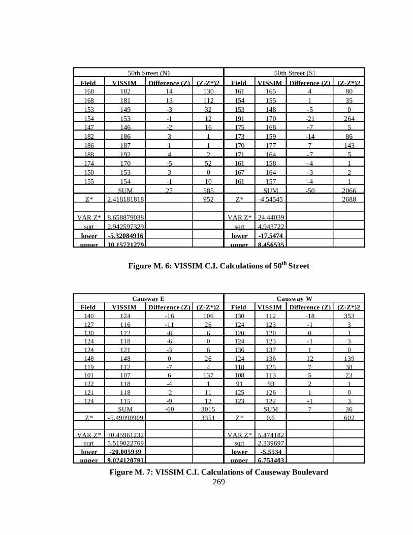
269
Field VISSIM Difference (Z) (Z-Z*)2 Field VISSIM Difference (Z) (Z-Z*)2168 182 14 130 161 165 4 80168 181 13 112 154 155 1 35153 149 -3 32 153 148 -5 0154 153 -1 12 191 170 -21 264147 146 -2 16 175 168 -7 5182 186 3 1 173 159 -14 86186 187 1 1 170 177 7 143188 192 4 2 171 164 -7 5174 170 -5 52 161 158 -4 1150 153 3 0 167 164 -3 2155 154 -1 10 161 157 -4 1
SUM 27 585 SUM -50 2066Z* 2.418181818 952 Z* -4.54545 2688
VAR Z* 8.658879038 VAR Z* 24.44039sqrt 2.942597329 sqrt 4.943722
lower -5.32084916 lower -17.5474upper 10.15721279 upper 8.456535
50th Street (S)50th Street (N)
Figure M. 6: VISSIM C.I. Calculations of 50th Street
Field VISSIM Difference (Z) (Z-Z*)2 Field VISSIM Difference (Z) (Z-Z*)2140 124 -16 106 130 112 -18 353127 116 -11 26 124 123 -1 3130 122 -8 6 120 120 0 1124 118 -6 0 124 123 -1 3124 121 -3 6 136 137 1 0148 148 0 26 124 136 12 139119 112 -7 4 118 125 7 38101 107 6 137 108 113 5 23122 118 -4 1 91 93 2 1121 118 -2 11 125 126 1 0124 115 -9 12 123 122 -1 3
SUM -60 3015 SUM 7 36Z* -5.49090909 3351 Z* 0.6 602
VAR Z* 30.45961232 VAR Z* 5.474182sqrt 5.519022769 sqrt 2.339697
lower -20.005939 lower -5.5534upper 9.024120791 upper 6.753403
Causway E Causway W
Figure M. 7: VISSIM C.I. Calculations of Causeway Boulevard

270
Field VISSIM Difference (Z) (Z-Z*)2 Field VISSIM Difference (Z) (Z-Z*)2184 179 -5 1 127 130 3 7196 192 -4 6 137 135 -1 2184 176 -8 4 142 137 -5 29182 179 -3 14 123 125 2 3164 167 3 91 120 132 11 130197 182 -14 61 126 126 1 0192 174 -18 145 150 154 4 16186 178 -8 3 133 128 -5 25184 178 -6 1 157 156 -1 2178 181 3 84 136 127 -9 74198 189 -9 9 121 123 2 3
SUM -70 4050 SUM 0 0Z* -6.36363636 4470 Z* 1.29E-15 290
VAR Z* 40.63392938 VAR Z* 2.638545sqrt 6.374474831 sqrt 1.62436
lower -23.1285052 lower -4.27207upper 10.40123244 upper 4.272067
22nd St. 21st St
Figure M. 8: VISSIM C.I. Calculations of 22nd and 21st Streets

271
APPENDIX N Forecasted Truck Volumes on Network Links for the Port of Tampa

272
Day Dates Total 22nd-st Street 20th Street Causeway Blvd Sutton Pendola point
Friday 7/1/05 4333 1244 553 1288 362 235
Monday 7/4/05 4329 1233 548 1275 358 233
Tuesday 7/5/05 4041 1254 557 1297 365 237
Wednesday 7/6/05 4292 1243 553 1287 361 235
Thursday 7/7/05 4385 1160 516 1201 337 219
Table N. 1: Forecast of Daily Number of Trucks Coming to the Port of Tampa in the First Week of July 2005
Day Dates Total 22nd-st Street 20th Street Causeway Blvd Sutton Pendola point
Friday 7/1/05 3689 863 547 1591 355 332
Monday 7/4/05 3929 779 494 1436 320 300
Tuesday 7/5/05 3337 944 598 1740 388 363
Wednesday 7/6/05 3330 919 582 1694 378 354
Thursday 7/7/05 4034 781 495 1439 321 301
Table N. 2: Forecast of Daily Number of Trucks Leaving the Port of Tampa in the First Week of July 2005

273
APPENDIX O VISSIM Runs Results for Sensitivity Analysis:
Average Travel Time and Average Delay of Network Links

274
Nodes # Description Link # DescriptionAvearge Travel
TimeAverage Delay State Road
1 U.S. Highway 41 / Madison Avenue 1 Node 1 to Node 2 115 10
2 78th street / Madison Avenue 2 Node 2 to Node 3 95 12
3 Madison Avenue / U.S. Highway 301 3 Node 3 to Node 4 92 15 SR 301
4 U.S. Highway 301 / I-75 4 Node 4 to Node 5 196 35 SR 301
5 State road 676 / U.S. Highway 301 5 Node 5 to Node 6 39 8 SR 301
6 Expressway 618 / U.S. Highway 301 6 Node 6 to Node 7 73 26 SR 301
7 State Highway 60 / U.S. Highway 301 7 Node 7 to Node 8 95 29 SR 301
8 State Highway 574 / U.S. Highway 301 8 Node 8 to Node 9 183 11
9 State Highway 574 / I-4 9 Node 9 to Node 10 125 10 I-4
10 22nd Street / I-4 10 Node 10 to Node 11 165 13 I-4
11 I-4 / I-275 11 Node 11 to Node 12 176 15 I-275
12 State Highway 92 / I-275 12 Node 12 to Node 13 34 9 SR 92
13 State Highway 92 / State Highway 60 13 Node 13 to Node 14 345 95 SR 92
14 State Highway 92 / State Highway 618 14 Node 14 to Node 15 234 15 SR 618
15 State Highway 60 / Expressway 618 15 Node 15 to Node 16 135 12 SR 618
16 22nd Street / Expressway 618 16 Node 16 to Node 17 127 10 SR 618
17 State Highway 41 / Expressway 618 17 Node 17 to Node 18 89 24 SR 41
18 State road 676 / U.S. Highway 41 18 Node 18 to Node 1 65 26 SR 41
19 State Highway 41 / State Highway 60 19 Node 19 to Node 17 25 6 SR 41
20 22nd Street / State Highway 60 20 Node 21 to Node 5 93 43 SR 676
21 State road 676 / 78th street 21 Node 2 to Node 21 73 28
22 Node 21 to Node 18 132 52 SR 676
23 Node 6 to Node 17 145 15 SR 618
24 Node 19 to Node 7 198 61 SR 60
25 Node 10 to Node 20 138 25
26 Node 20 to Node 16 43 13
27 Node 19 to Node 20 216 73 SR 60
28 Node 15 to Node 20 183 29 SR 60
29 Node 13 to Node 15 354 203 SR 60
30 Node 9 to Node 19 113 27 SR 41
Table O. 1: Scenario 1 (Base Scenario)
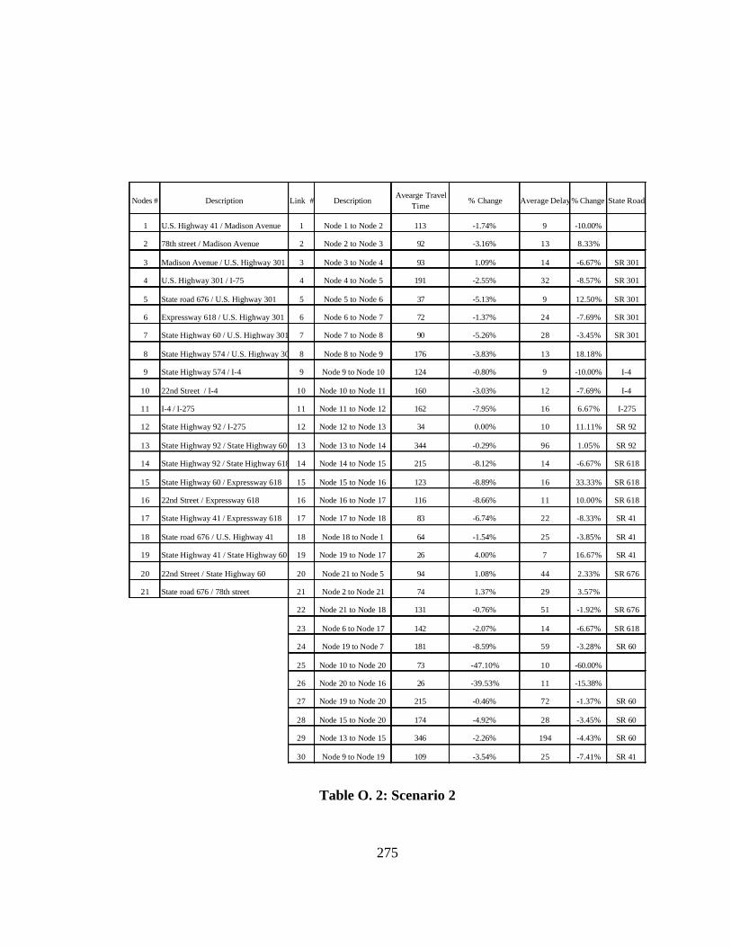
275
Nodes # Description Link # DescriptionAvearge Travel
Time% Change Average Delay% Change State Road
1 U.S. Highway 41 / Madison Avenue 1 Node 1 to Node 2 113 -1.74% 9 -10.00%
2 78th street / Madison Avenue 2 Node 2 to Node 3 92 -3.16% 13 8.33%
3 Madison Avenue / U.S. Highway 301 3 Node 3 to Node 4 93 1.09% 14 -6.67% SR 301
4 U.S. Highway 301 / I-75 4 Node 4 to Node 5 191 -2.55% 32 -8.57% SR 301
5 State road 676 / U.S. Highway 301 5 Node 5 to Node 6 37 -5.13% 9 12.50% SR 301
6 Expressway 618 / U.S. Highway 301 6 Node 6 to Node 7 72 -1.37% 24 -7.69% SR 301
7 State Highway 60 / U.S. Highway 301 7 Node 7 to Node 8 90 -5.26% 28 -3.45% SR 301
8 State Highway 574 / U.S. Highway 301 8 Node 8 to Node 9 176 -3.83% 13 18.18%
9 State Highway 574 / I-4 9 Node 9 to Node 10 124 -0.80% 9 -10.00% I-4
10 22nd Street / I-4 10 Node 10 to Node 11 160 -3.03% 12 -7.69% I-4
11 I-4 / I-275 11 Node 11 to Node 12 162 -7.95% 16 6.67% I-275
12 State Highway 92 / I-275 12 Node 12 to Node 13 34 0.00% 10 11.11% SR 92
13 State Highway 92 / State Highway 60 13 Node 13 to Node 14 344 -0.29% 96 1.05% SR 92
14 State Highway 92 / State Highway 618 14 Node 14 to Node 15 215 -8.12% 14 -6.67% SR 618
15 State Highway 60 / Expressway 618 15 Node 15 to Node 16 123 -8.89% 16 33.33% SR 618
16 22nd Street / Expressway 618 16 Node 16 to Node 17 116 -8.66% 11 10.00% SR 618
17 State Highway 41 / Expressway 618 17 Node 17 to Node 18 83 -6.74% 22 -8.33% SR 41
18 State road 676 / U.S. Highway 41 18 Node 18 to Node 1 64 -1.54% 25 -3.85% SR 41
19 State Highway 41 / State Highway 60 19 Node 19 to Node 17 26 4.00% 7 16.67% SR 41
20 22nd Street / State Highway 60 20 Node 21 to Node 5 94 1.08% 44 2.33% SR 676
21 State road 676 / 78th street 21 Node 2 to Node 21 74 1.37% 29 3.57%
22 Node 21 to Node 18 131 -0.76% 51 -1.92% SR 676
23 Node 6 to Node 17 142 -2.07% 14 -6.67% SR 618
24 Node 19 to Node 7 181 -8.59% 59 -3.28% SR 60
25 Node 10 to Node 20 73 -47.10% 10 -60.00%
26 Node 20 to Node 16 26 -39.53% 11 -15.38%
27 Node 19 to Node 20 215 -0.46% 72 -1.37% SR 60
28 Node 15 to Node 20 174 -4.92% 28 -3.45% SR 60
29 Node 13 to Node 15 346 -2.26% 194 -4.43% SR 60
30 Node 9 to Node 19 109 -3.54% 25 -7.41% SR 41
Table O. 2: Scenario 2

276
Nodes # Description Link # DescriptionAvearge Travel
Time % Change Average Delay % Change State Road
1 U.S. Highway 41 / Madison Avenue 1 Node 1 to Node 2 117 1.74% 11 10.00%
2 78th street / Madison Avenue 2 Node 2 to Node 3 97 2.11% 13 8.33%
3 Madison Avenue / U.S. Highway 301 3 Node 3 to Node 4 93 1.09% 16 6.67% SR 301
4 U.S. Highway 301 / I-75 4 Node 4 to Node 5 198 1.02% 37 5.71% SR 301
5 State road 676 / U.S. Highway 301 5 Node 5 to Node 6 41 5.13% 10 25.00% SR 301
6 Expressway 618 / U.S. Highway 301 6 Node 6 to Node 7 89 21.92% 38 46.15% SR 301
7 State Highway 60 / U.S. Highway 301 7 Node 7 to Node 8 112 17.89% 31 6.90% SR 301
8 State Highway 574 / U.S. Highway 301 8 Node 8 to Node 9 198 8.20% 15 36.36%
9 State Highway 574 / I-4 9 Node 9 to Node 10 123 -1.60% 11 10.00% I-4
10 22nd Street / I-4 10 Node 10 to Node 11 162 -1.82% 12 -7.69% I-4
11 I-4 / I-275 11 Node 11 to Node 12 178 1.14% 16 6.67% I-275
12 State Highway 92 / I-275 12 Node 12 to Node 13 35 2.94% 9 0.00% SR 92
13 State Highway 92 / State Highway 60 13 Node 13 to Node 14 359 4.06% 103 8.42% SR 92
14 State Highway 92 / State Highway 618 14 Node 14 to Node 15 243 3.85% 20 33.33% SR 618
15 State Highway 60 / Expressway 618 15 Node 15 to Node 16 137 1.48% 12 0.00% SR 618
16 22nd Street / Expressway 618 16 Node 16 to Node 17 135 6.30% 13 30.00% SR 618
17 State Highway 41 / Expressway 618 17 Node 17 to Node 18 92 3.37% 27 12.50% SR 41
18 State road 676 / U.S. Highway 41 18 Node 18 to Node 1 67 3.08% 27 3.85% SR 41
19 State Highway 41 / State Highway 60 19 Node 19 to Node 17 27 8.00% 8 33.33% SR 41
20 22nd Street / State Highway 60 20 Node 21 to Node 5 96 3.23% 45 4.65% SR 676
21 State road 676 / 78th street 21 Node 2 to Node 21 72 -1.37% 27 -3.57%
22 Node 21 to Node 18 134 1.52% 57 9.62% SR 676
23 Node 6 to Node 17 159 9.66% 24 60.00% SR 618
24 Node 19 to Node 7 218 10.10% 73 19.67% SR 60
Table O. 3: Scenario 3
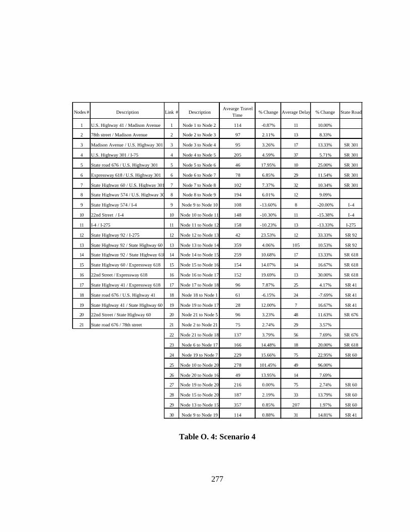
277
Nodes # Description Link # DescriptionAvearge Travel
Time% Change Average Delay % Change State Road
1 U.S. Highway 41 / Madison Avenue 1 Node 1 to Node 2 114 -0.87% 11 10.00%
2 78th street / Madison Avenue 2 Node 2 to Node 3 97 2.11% 13 8.33%
3 Madison Avenue / U.S. Highway 301 3 Node 3 to Node 4 95 3.26% 17 13.33% SR 301
4 U.S. Highway 301 / I-75 4 Node 4 to Node 5 205 4.59% 37 5.71% SR 301
5 State road 676 / U.S. Highway 301 5 Node 5 to Node 6 46 17.95% 10 25.00% SR 301
6 Expressway 618 / U.S. Highway 301 6 Node 6 to Node 7 78 6.85% 29 11.54% SR 301
7 State Highway 60 / U.S. Highway 301 7 Node 7 to Node 8 102 7.37% 32 10.34% SR 301
8 State Highway 574 / U.S. Highway 301 8 Node 8 to Node 9 194 6.01% 12 9.09%
9 State Highway 574 / I-4 9 Node 9 to Node 10 108 -13.60% 8 -20.00% I-4
10 22nd Street / I-4 10 Node 10 to Node 11 148 -10.30% 11 -15.38% I-4
11 I-4 / I-275 11 Node 11 to Node 12 158 -10.23% 13 -13.33% I-275
12 State Highway 92 / I-275 12 Node 12 to Node 13 42 23.53% 12 33.33% SR 92
13 State Highway 92 / State Highway 60 13 Node 13 to Node 14 359 4.06% 105 10.53% SR 92
14 State Highway 92 / State Highway 618 14 Node 14 to Node 15 259 10.68% 17 13.33% SR 618
15 State Highway 60 / Expressway 618 15 Node 15 to Node 16 154 14.07% 14 16.67% SR 618
16 22nd Street / Expressway 618 16 Node 16 to Node 17 152 19.69% 13 30.00% SR 618
17 State Highway 41 / Expressway 618 17 Node 17 to Node 18 96 7.87% 25 4.17% SR 41
18 State road 676 / U.S. Highway 41 18 Node 18 to Node 1 61 -6.15% 24 -7.69% SR 41
19 State Highway 41 / State Highway 60 19 Node 19 to Node 17 28 12.00% 7 16.67% SR 41
20 22nd Street / State Highway 60 20 Node 21 to Node 5 96 3.23% 48 11.63% SR 676
21 State road 676 / 78th street 21 Node 2 to Node 21 75 2.74% 29 3.57%
22 Node 21 to Node 18 137 3.79% 56 7.69% SR 676
23 Node 6 to Node 17 166 14.48% 18 20.00% SR 618
24 Node 19 to Node 7 229 15.66% 75 22.95% SR 60
25 Node 10 to Node 20 278 101.45% 49 96.00%
26 Node 20 to Node 16 49 13.95% 14 7.69%
27 Node 19 to Node 20 216 0.00% 75 2.74% SR 60
28 Node 15 to Node 20 187 2.19% 33 13.79% SR 60
29 Node 13 to Node 15 357 0.85% 207 1.97% SR 60
30 Node 9 to Node 19 114 0.88% 31 14.81% SR 41
Table O. 4: Scenario 4

278
APPENDIX P Scheffe’s Test for Port Canaveral Freight Terminal Daily Truck Volumes

279
South-in
Scheffea,b
14 71.7916 114.88
14 225.4315 246.6717 251.8218 255.44
17 266.47.220 .275
DAYSUNDAY
SATURDAYMONDAYTUESDAYWEDNESDAYFRIDAY
THURSDAYSig.
N 1 2Subset for alpha = .05
Means for groups in homogeneous subsets are displayed.
Uses Harmonic Mean Sample Size = 15.722.a.
The group sizes are unequal. The harmonic meanof the group sizes is used. Type I error levels arenot guaranteed.
b.
Figure P. 1: South Terminal (Inbound)
North-in
Scheffea,b
14 1.8616 14.25
14 96.2918 103.1715 108.7317 115.82
17 120.06.823 .115
DAYSUNDAY
SATURDAYMONDAYFRIDAYTUESDAYTHURSDAY
WEDNESDAYSig.
N 1 2Subset for alpha = .05
Means for groups in homogeneous subsets are displayed.
Uses Harmonic Mean Sample Size = 15.722.a.
The group sizes are unequal. The harmonic meanof the group sizes is used. Type I error levels arenot guaranteed.
b.
Figure P. 2: North Terminal (Inbound)

280
South-out
Scheffea,b
13 57.6915 88.80
11 186.2713 199.5412 207.0815 208.67
13 213.85.804 .880
DAYSUNDAY
SATURDAYMONDAYFRIDAYTHURSDAYWEDNESDAY
TUESDAYSig.
N 1 2Subset for alpha = .05
Means for groups in homogeneous subsets are displayed.
Uses Harmonic Mean Sample Size = 13.003.a.
The group sizes are unequal. The harmonic meanof the group sizes is used. Type I error levels arenot guaranteed.
b.
Figure P. 3: South Terminal (Outbound)
North-out
Scheffea,b
13 3.4615 14.47
11 110.0013 110.5412 120.3313 121.46
16 133.69.916 .169
DAYSUNDAY
SATURDAYMONDAYFRIDAYTHURSDAYTUESDAY
WEDNESDAYSig.
N 1 2Subset for alpha = .05
Means for groups in homogeneous subsets are displayed.
Uses Harmonic Mean Sample Size = 13.104.a.
The group sizes are unequal. The harmonic meanof the group sizes is used. Type I error levels arenot guaranteed.
b.
Figure P. 4: North Terminal (Outbound)

281
APPENDIX Q Statistical Results for Port Canaveral ANN Validation Data
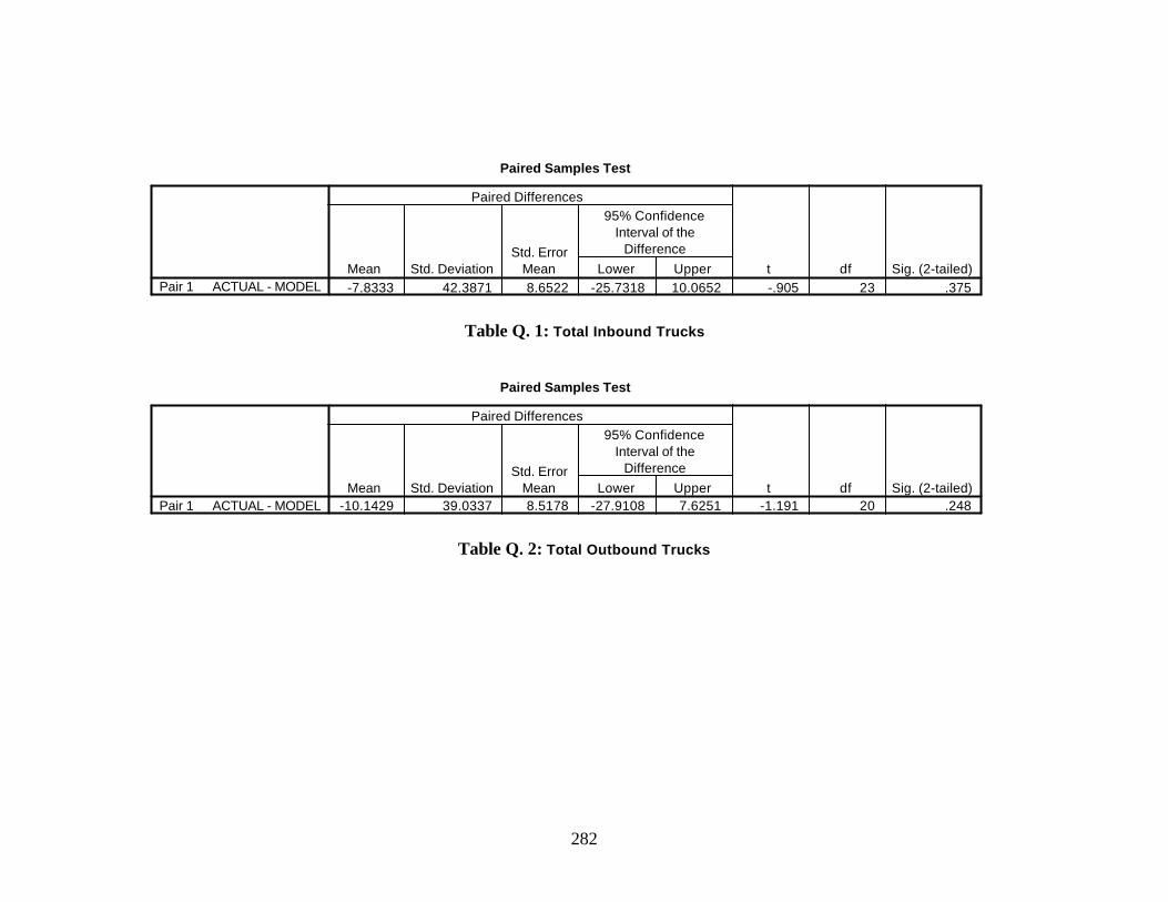
282
Paired Samples Test
-7.8333 42.3871 8.6522 -25.7318 10.0652 -.905 23 .375ACTUAL - MODELPair 1Mean Std. Deviation
Std. ErrorMean Lower Upper
95% ConfidenceInterval of the
Difference
Paired Differences
t df Sig. (2-tailed)
Table Q. 1: Total Inbound Trucks
Paired Samples Test
-10.1429 39.0337 8.5178 -27.9108 7.6251 -1.191 20 .248ACTUAL - MODELPair 1Mean Std. Deviation
Std. ErrorMean Lower Upper
95% ConfidenceInterval of the
Difference
Paired Differences
t df Sig. (2-tailed)
Table Q. 2: Total Outbound Trucks
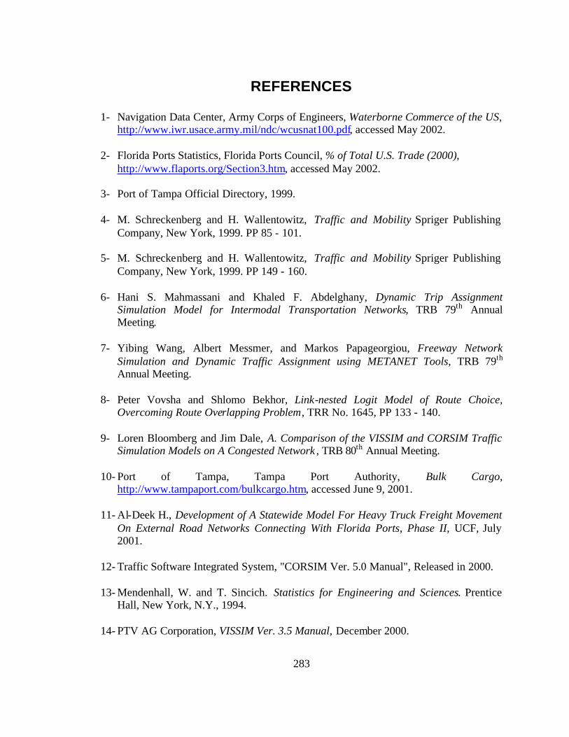
283
REFERENCES 1- Navigation Data Center, Army Corps of Engineers, Waterborne Commerce of the US,
http://www.iwr.usace.army.mil/ndc/wcusnat100.pdf, accessed May 2002. 2- Florida Ports Statistics, Florida Ports Council, % of Total U.S. Trade (2000),
http://www.flaports.org/Section3.htm, accessed May 2002. 3- Port of Tampa Official Directory, 1999. 4- M. Schreckenberg and H. Wallentowitz, Traffic and Mobility Spriger Publishing
Company, New York, 1999. PP 85 - 101. 5- M. Schreckenberg and H. Wallentowitz, Traffic and Mobility Spriger Publishing
Company, New York, 1999. PP 149 - 160. 6- Hani S. Mahmassani and Khaled F. Abdelghany, Dynamic Trip Assignment
Simulation Model for Intermodal Transportation Networks, TRB 79th Annual Meeting.
7- Yibing Wang, Albert Messmer, and Markos Papageorgiou, Freeway Network
Simulation and Dynamic Traffic Assignment using METANET Tools, TRB 79th Annual Meeting.
8- Peter Vovsha and Shlomo Bekhor, Link-nested Logit Model of Route Choice,
Overcoming Route Overlapping Problem, TRR No. 1645, PP 133 - 140. 9- Loren Bloomberg and Jim Dale, A. Comparison of the VISSIM and CORSIM Traffic
Simulation Models on A Congested Network , TRB 80th Annual Meeting. 10- Port of Tampa, Tampa Port Authority, Bulk Cargo,
http://www.tampaport.com/bulkcargo.htm, accessed June 9, 2001. 11- Al-Deek H., Development of A Statewide Model For Heavy Truck Freight Movement
On External Road Networks Connecting With Florida Ports, Phase II, UCF, July 2001.
12- Traffic Software Integrated System, "CORSIM Ver. 5.0 Manual", Released in 2000. 13- Mendenhall, W. and T. Sincich. Statistics for Engineering and Sciences. Prentice
Hall, New York, N.Y., 1994. 14- PTV AG Corporation, VISSIM Ver. 3.5 Manual, December 2000.

284
15- Adolf D. May ,Traffic Flow Fundamentals, Prentice-Hall, New Jersey, 1990


![Bosch ESI[truck] Heavy Duty Truck Software Update – Q1 ...€¦ · Bosch ESI[truck] Heavy Duty Truck Software Update | Ver 2019/1 6 | 41 41135 42908 45411 47482 37000 38000 39000](https://img.dokumen.tips/doc/110x75/600ed0e779e62601223e82fb/bosch-esitruck-heavy-duty-truck-software-update-a-q1-bosch-esitruck-heavy.jpg)


![Bosch ESI[truck] Heavy Duty Truck Software Update – Q1](https://img.dokumen.tips/doc/110x75/61bd27cf61276e740b0fedf7/bosch-esitruck-heavy-duty-truck-software-update-q1-.jpg)