1

Development of a Process Model for the Vacuum Assisted Resin Transfer Molding Simulation by the Response Surface

Method

Chensong (Jonathan) Dong *

Rakon Limited

One Pacific Rise, Mt. Wellington Private Bag 99943, Newmarket

Auckland, New Zealand chensongdong@yahoo.com

Abstract The vacuum assisted resin transfer molding process (VARTM) offers many

advantages over the traditional resin transfer molding such as lower tooling cost, room

temperature processing. In the VARTM process, complete filling of the mold with

adequate wetting of the fibrous preform is critical to the product quality. Computer

simulation has become a powerful tool for liquid composite molding process design and

optimization. However, in the VARTM process, since the presence of High Permeable

Media (HPM), which has a much higher permeability than fiber, 3-D models are

necessary and the extensive computation limits the usage of simulation in the process

design and optimization.

With the permeability, porosity, and thickness of the fiber preform and the RTM

mold filling time as references, the dimensionless VARTM process variables and mold

filling time are introduced in this paper. The significant process variables were identified

by using the Design of Experiments (DOE). A quadratic regression model was

developed by the RSM. The model was validated against the 3-D VARTM simulation

* To whom all correspondence should be addressed.

2

and experiments. The results show that the accuracy is within 15% for most commonly

used cases while the computation time saving is over 99%. The approach presented in

this paper provides a general guideline for the VARTM process design and optimization.

The process variables and flow media can be quickly chosen by using the developed

regression model, which is extremely useful for composite part design in the early stage.

Keywords: E: resin flow; C: computational modeling; High Permeable Medium

(HPM); Response Surface Method (RSM)

1 Introduction The vacuum assisted resin transfer molding process (VARTM) offers many

advantages over the traditional resin transfer molding such as lower tooling cost, room

temperature processing. This process has been employed to manufacture many large

components ranging from turbine blades and boats to rail cars and bridge decks.

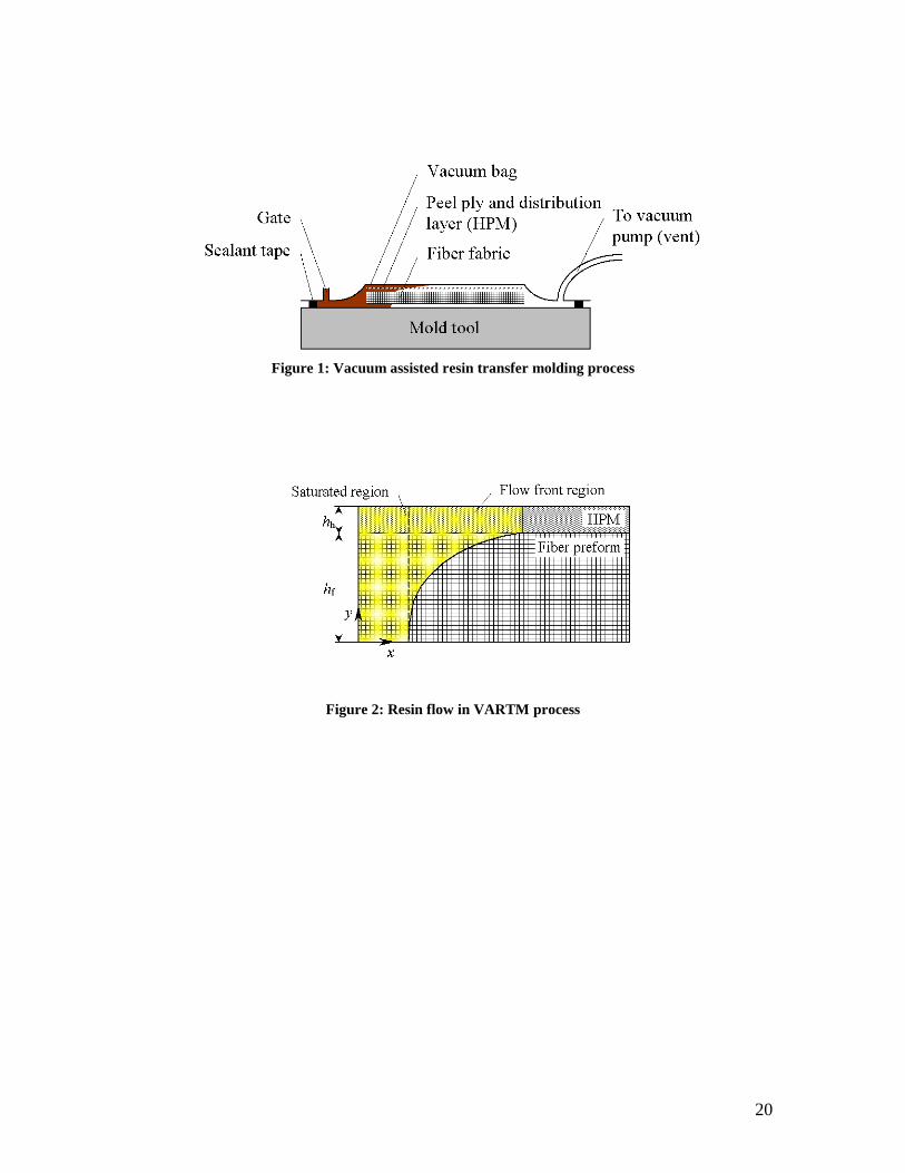
The VARTM process can be divided into five steps. First, in pre-molding, the

mold surface is cleaned. Then mold release agent and gel coat are sprayed onto the

surface. Next, during reinforcement loading, dry fiber mats are mounted into the mold

and covered by a flexible bag film. The cavity is sealed, e.g. by vacuum tapes. Vacuum

is created in the mold cavity to draw the resin into the fiber mats. After the cavity is

filled with resin, the resin cures and solidifies into the composite part. Finally, the

solidified composite is taken out of the mold. Although this process appears simple, in

actual fabrication, the procedure can be quite complicated. The locations of the inlets and

3

outlets must be carefully selected so that the mold can be completely filled. The mold

and resin temperature must be monitored to avoid resin gelling during resin infusion.

This study focuses on one of the common VARTM processes: the Seemann

Composite Resin Infusion Molding Process (SCRIMP), which was invented and patented

in the late 1980’s by Bill Seemann. In this process, a highly permeable distribution

medium is incorporated into fiber preform as a surface layer. During infusion, resin

flows preferentially across the surface and simultaneously through the preform thickness,

which enables large parts to be fabricated.

Complete filling of the mold with adequate wetting of the fibrous preform is

critical in the VARTM. Incomplete impregnation in the mold leads to defective parts

containing dry spots. In order to achieve good quality, processing parameters such as the

locations and numbers of gates and vents need to be properly set.

Traditionally, trial-and-error techniques are widely applied in the composite

industry, which largely depend on the experience and skills of operators. It is very costly

and time consuming. With the development of computing technology, simulation has

become a powerful tool for the process design and optimization. The Control Volume

Finite Element Method (CVFEM) has been the predominant method for process

simulation [1-6]. It forms and solves a set of equations for nodal control volumes as if

they were finite elements. Mesh regeneration is not required, which makes the

computation more efficient.

In the conventional RTM process, fiber is the only flow medium. The part can

often be regarded as a shell and simulation in 2-D domain. The simulation techniques are

quite developed and several commercial simulation software packages are available [7-

4

10]. In the VARTM process, due to the existence of two distinct flow media, fiber

preform and High Permeable Medium (HPM), usually 3-D models are required for

simulation.

When a 3-D model is used, for large parts, the VARTM simulation requires a

large number of nodes and elements during meshing. In addition, the distribution

medium is usually much thinner than the preform. Therefore, a finer mesh is needed to

avoid the high aspect ratio, which may result in poor conditioning in simulation, as well

as from discretization errors. This uses a large amount of computer hardware resources

and increases the computer load. The simulation time increases significantly and makes

the simulation not feasible.

VARTM simulation has been studied extensively. Mathur et al. [11] developed

an analytical model, which predicts the flow times and flow front shapes as a function of

the properties of the preform, distribution media and resin. Further, they formulated a

performance index to give a measure of the process efficacy. Loos et al. [12] developed

a 3-D model to simulate the VARTM manufacturing process of complex shape composite

structures. Mohan et al. [13] modeled and characterized the flow in channels using

equivalent permeability. The equivalent permeability is used as input for numerical

simulation of the mold filling process. The numerical simulations are based on a pure

finite element based methodology. The mold filling in the VARTM was investigated by

Sun et al. [14] based on a High Permeable Medium and Ni [15] et al. based on grooves.

A 3-D Control Volume Finite Element Method was adopted to solve the flow governing

equations. Based on experimental observations and CVFEM simulation, a simplified

leakage flow model was presented, where they considered the preform and the peel ply as

5

a sink for the resin, while modeling the flow in the distribution layer. Tari et al. [16]

derived a closed form model for vacuum bag resin transfer molding under several

simplifying assumptions. They assumed that the resin velocity in the saturated fiber

preform is negligible. Hsiao et al. [17] avoided this assumption and hence the velocity

for the resin, as well as the shape of the flow front through the thickness of the fiber

preform, was accurately captured. Han et al. [18] proposed a hybrid 2.5-D and 3-D flow

model. Dong [19] presented an Equivalent Medium Method for improving computation

efficiency of the VARTM simulation.

From the literature survey, most of the studies focused on the development of

simplified models due to the extensive computations involved in the 3-D CVFEM

method. However, the 3-D nature of VARTM simulation is not avoided. Thus, the

simulation is more time-consuming than 2-D RTM simulation. In addition, the 3-D

Finite Element modeling and material defining process are more complicated due to the

anisotropic nature of flow media. The fiber direction needs to be specified for each

element to relate the material orientation to the coordinate system, as shown in Figure 2.

In view of the industrial application, the mold filling process and time need to be

predicted in a timely manner to reduce the lead time. The 3-D simulation is incapable of

meeting this requirement. Thus, it is necessary to develop a more convenient tool for

VARTM simulation.

Dimensionless VARTM process variables including dimensionless permeability,

porosity, and thickness have been introduced in this paper. The dimensionless VARTM

mold filling time was also derived by correlating the VARTM process with the RTM

process. The significant process variables were identified by using the Design of

6

Experiments (DOE). A quadratic regression model was developed by the RSM. The

VARTM mold filling time can be obtained by multiplying the RTM mold filling time of

the same composite part by the dimensionless VARTM mold filling time. The model

was validated against the 3-D VARTM simulation and experiments. The results show

that the accuracy is within 10% for most commonly used cases while the computation

time saving is over 99%. The original contributions of this research are:

1. A guideline for VARTM process design is provided. The process parameters can

be selected per this guideline.

2. An efficient and effective approach is developed for the VARTM process

optimization. By using this approach, the process parameters can be found to

meet the objective in a time-efficient way.

3. Since variations exist for the process parameters [20], the approach presented in

this paper can also be used as a robust design tool to reduce the sensitivity to the

variations of process parameters.

The rest of the paper is structured as follows. In section 2, the approach to

develop a VARTM process regression model is presented. The model validation is

presented in Section 3. Section 4 discusses the application of the presented model.

Conclusions are drawn in Section 5.

2 Approach

2.1 Control Volume Finite Element Method (CVFEM)

The flow of a viscous fluid through an anisotropic, homogenous, porous medium

is represented by Darcy’s law [21]:

7

( )

∂∂∂∂∂∂

−=

zpypxp

KKKKKKKKK

wvu

zzzyzx

yzyyyx

xzxyxx

µ1 (1)

where Kij (i, j = x, y, or z) are the components of the permeability tensor. ∂p/∂x, ∂p/∂y

and ∂p/∂z are the pressure gradients in the three directions respectively.

For an incompressible fluid, the mass conservation equation can be reduced to the

form:

0=∂∂+∂∂+∂∂ zwyvxu . (2)

Equation 2 can be integrated over a control volume and leads to:

( ) 0=∂∂+∂∂+∂∂∫∫∫V

dVzwyvxu . (3)

Using the Divergence theorem (Gauss’s theorem), the control volume integral can

be transformed into a control surface integral. Thus, Equation 3 can be written as:

0=

∫∫S

zyx dSwvu

nnn (4)

where nx, ny and nz are the normal components of the surface vector of the control volume.

Substituting Equation 1 into Equation 4 yields:

( ) 01 =

∂∂∂∂∂∂

∫∫S

zzzyzx

yzyyyx

xzxyxx

zyx dSzpypxp

KKKKKKKKK

nnnµ . (5)

Equation 5 is the working equation for solving the problems of flow through

anisotropic porous media and is a combination of the mass and momentum equations,

while the momentum equation is represented by using the Darcy’s law.

8

In order to solve such moving boundary problems as the resin flow front advances

using the traditional finite element method, it requires the computation domain

redefinition and mesh regeneration. Mesh regeneration needs a large amount of

computation time as the domain becomes complicated. Alternatively, the control volume

finite element method, which forms and solves a set of equations for nodal control

volumes as if they were finite elements, does not require mesh regeneration. Thus, the

computation is more efficient.

The boundary conditions for mold filling simulation are as follows:

At the flow front:

0=p . (6)

At the inlet gates:

For constant pressure: 0pp = ; (7)

For the constant flow rate: 0vv = . (8)

At the mold boundaries:

0=∂∂ np . (9)

It is assumed that at the beginning of mold filling, the control volumes enclosing

the inlet nodes are filled with resin. At the flow front, a parameter f is used to represent

the status of each control volume in the flow domain. If the control volume has not been

occupied by the fluid, f is equal to zero. If the control volume is partially filled, f is equal

to the volume fraction of the fluid occupying the control volume. f factor is set to 1 if the

volume is completely filled by advancing fluid. The control volumes with f values

varying between 0 and 1 are considered flow front elements. The pressure in these

partially filled flow front control volumes is set to the ambient pressure. With the

9

aforementioned boundary conditions, the set of linear algebraic equations can be solved

to determine the pressure field at each time step during mold filling. Based on the

calculated pressure field, the velocity field can then be computed using Darcy’s law.

The time increment is selected in such a way that a control volume will be fill at

each time step. Sometimes, several control volumes can be filled simultaneously. After f

values are updated, another pressure computation is performed for all the fully filled

control volumes. The process is repeated until the whole mold is filled [2].

2.2 RTM and VARTM Simulation

In the traditional RTM process, fiber preform is the only flow medium. The

through-thickness resin flow can often be neglected and thus a 2-D model can be applied.

In the VARTM process, however, another flow medium — High Permeable Medium

(HPM) presents. Considering a 1-D flow in the VARTM process, the resin flow front is

plotted in Figure 2. The HPM is much thinner than the preform. The flow is assumed to

be well developed and can be divided into two regions: saturated region and flow front

region. In the saturated region, no cross-flow exists, while in the flow front region the

resin is infiltrating into the preform from the HPM.

When the inputs in the CVFEM mold filling simulation are considered, they can

be divided into:

• Geometric properties: molding geometry

• Material properties: permeability and porosity

• Condition properties: injection method and pressure, viscosity of resin

The closed form solution for the 1-D flow through a homogeneous fiber preform

can be derived from Darcy’s law as

10

( )Kplt 02 2φµ= . (10)

Expanded to the general case, it can be derived that

( )Kpt 0φµ∝ . (11)

If the reference variables are φref, µref, p0ref and Kref, and the reference mold filling time is

tref, Equation 11 can be written as

( )[ ] ( )[ ]refrefrefrefref KpKptt 00 µφφµ= (12)

When the material properties of fiber are considered as the only variables, Equation 12

becomes

( ) ( )refrefref KKtt φφ= (13)

In the VARTM process, two types of flow media — fiber preform and HPM exist.

If the properties of fiber preforms and the RTM mold filling time are regarded as the

reference variables and mold filling time, respectively, the VARTM mold filling time can

be derived by using Equation 13 as

( ) ( )[ ] ( )ffHfHfHfHf KhhKKFhhFtt φφφ ,,,,,, 21RTMVARTM = (14)

Equation 14 shows that the VARTM mold filling time is dependent on the

permeability and porosity of fiber preform and HPM, and the composition of fiber

preform and HPM. It can be further written as

( ) ( )[ ]fHfHfHfH hhKKGhhGtt ,, 21RTMVARTM φφ= (15)

If the dimensionless process variables for the VARTM process are derived as

fH KKK =* , fH φφφ =* , fH hhh =* , and the dimensionless VARTM mold filling

time is given by the VARTM-RTM mold filling time ratio as RTMVARTM* ttt = , Equation

15 becomes

11

( ) ( )[ ]**2

**1RTMVARTM ,, hKGhGtt φ= (16)

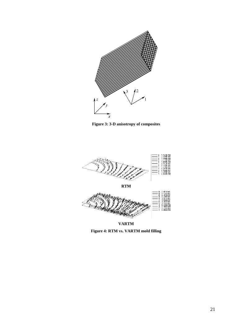
As a preliminary study, several RTM and VARTM mold filling process

simulation for the same part by both linear and port injection was simulated. For RTM

simulation, 2-D models were used and for VARTM simulation 3-D models were used.

The permeability was considered as the only variable. The thickness is 4 mm for the

fiber preform and 1 mm for the HPM. The porosity is 0.5 for the fiber preform and 0.8

for the HPM. The injection pressure is 1×105 Pa. When the permeability of the fiber

preform and HPM is 100 Darcy and 3,000 Darcy, respectively, the RTM and VARTM

mold filling process is shown in Figure 4. The complete result for various permeability

values is shown in Table 1. Thus, it is confirmed that the dimensionless mold filling time

is dependent on *φ , *h and *K . For a VARTM manufacturer, the microscopic level

through-thickness flow is usually of less importance than the in-plane resin flow front

development and mold filling time. Thus, it is possible to use 2-D RTM simulation and

dimensionless VARTM process variables to simulate the mold filling time.

The approach is illustrated in Figure 5. For any given composite part design, the

mold filling process can be simulated in 2-D using the RTM assumption. The

dimensionless VARTM process variables *φ , *h and *K are calculated and the

dimensionless VARTM mold filling time *t is calculated by the developed VARTM

process model. The actual VARTM mold filling time can be given by

RTM*

VARTM ttt = . (17)

12

2.3 Screening Design

First, a screening design was conducted to uncover the individual contributions to

the VARTM mold filling time of hH, φH and KH. A factorial design was conducted to

identify the significant factors.

Normally, the permeability is 50~200 Darcy for fiber preforms and 1,000~5,000

Darcy for HPM. The porosity is 0.4~0.6 for fiber preforms and 0.7~0.9 for HPM. The

thickness of HPM is less than 1 mm. In order to derive the dimensionless variables, Kf,

φf and hf were fixed at 100 Darcy, 0.5, and 4 mm, respectively. The levels of hH, φH and

KH are shown in Table 2. These were chosen to cover the normal application range. The

dimensionless VARTM process variables were derived and the dimensionless VARTM

mold filling time is the response.

A full 23 factorial design with center points were chosen. After data analysis, the

half normal plot, the main effects and interaction plots are shown in Figure 6. It shows

that the significant factors are: h*, K*, and the interaction of h* and K*. The ANOVA also

indicates that a significant curvature exists.

2.4 Model Development by Response Surface Method (RSM)

The result from the screening design shows that φ* is an insignificant variable so

that only h*, K* are used in the further analysis.

The significant effect of curvature indicates that a linear model is not sufficient.

A second-order response surface model needs to be developed. One effective way to

develop such a model is the Central Composite Design (CCD). Thus, the design was

augmented into a 22 design with four axial runs as shown in Figure 7.

13

The Box-Cox Method [22] was used to stabilize the variance. An inverse

transformation of the flow time was chosen. The final fitted regression model is

( )**12

2*22

2*11

*2

*10

* 1 KhaKahaKahaat +++++= , (18)

where

112

522

111

22

1

10

1001.5

1035.5

1084.1

1050.4

62.81051.1

−

−

−

−

×=

×−=

×−=

×=

=×−=

aaaaaa

.

Its corresponding response surface is shown in Figure 8.

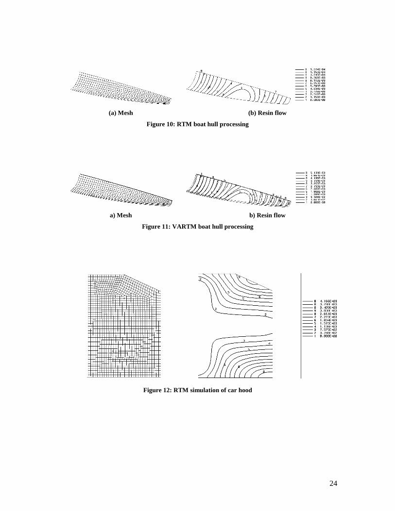
3 Model Validation A boat hull as shown in Figure 9 was simulated to validate the regression model.

Its length is 2 m.

The permeability is 80 Darcy for the fiber preform and 3,000 Darcy for the HPM.

The porosity is 0.5 for the fiber preform and 0.9 for the HPM the porosity.

First, the thickness of the fiber preform was assumed to be 20 mm. The

processing of the boat hull by the RTM process was simulated by using a 2-D CVFEM

model. Half of the structure was modeled due to its symmetry, as shown in Figure 10(a).

The injection pressure was 1×105 Pa. The viscosity was 200 cP. The mold filling

process is shown in Figure 10(b). The mold filling time is 13,903 sec.

When the VARTM processing of the boat hull was considered, the thickness of

the HPM was assumed to be 1 mm. The dimensionless variables were calculated as

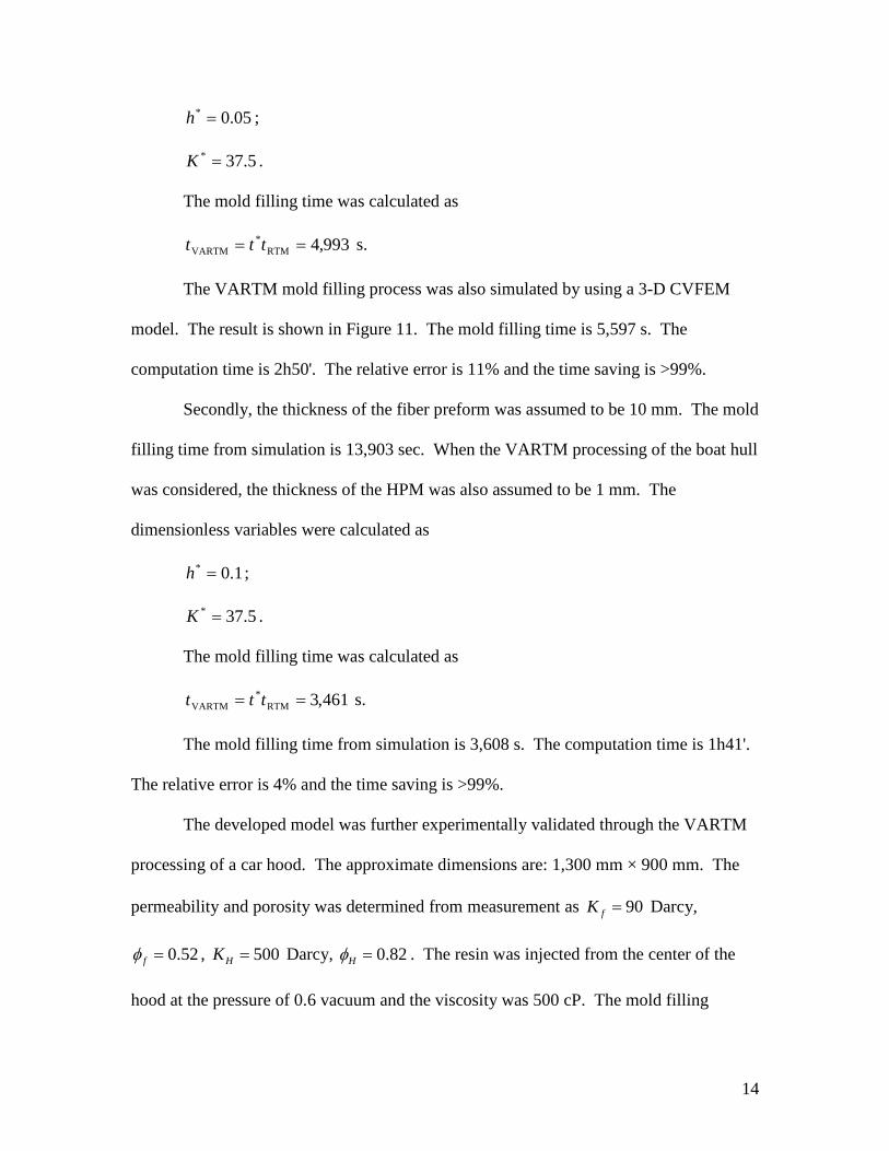
14

05.0* =h ;

5.37* =K .

The mold filling time was calculated as

993,4RTM*

VARTM == ttt s.

The VARTM mold filling process was also simulated by using a 3-D CVFEM

model. The result is shown in Figure 11. The mold filling time is 5,597 s. The

computation time is 2h50'. The relative error is 11% and the time saving is >99%.

Secondly, the thickness of the fiber preform was assumed to be 10 mm. The mold

filling time from simulation is 13,903 sec. When the VARTM processing of the boat hull

was considered, the thickness of the HPM was also assumed to be 1 mm. The

dimensionless variables were calculated as

1.0* =h ;

5.37* =K .

The mold filling time was calculated as

461,3RTM*

VARTM == ttt s.

The mold filling time from simulation is 3,608 s. The computation time is 1h41'.

The relative error is 4% and the time saving is >99%.

The developed model was further experimentally validated through the VARTM

processing of a car hood. The approximate dimensions are: 1,300 mm × 900 mm. The

permeability and porosity was determined from measurement as 90=fK Darcy,

52.0=fφ , 500=HK Darcy, 82.0=Hφ . The resin was injected from the center of the

hood at the pressure of 0.6 vacuum and the viscosity was 500 cP. The mold filling

15

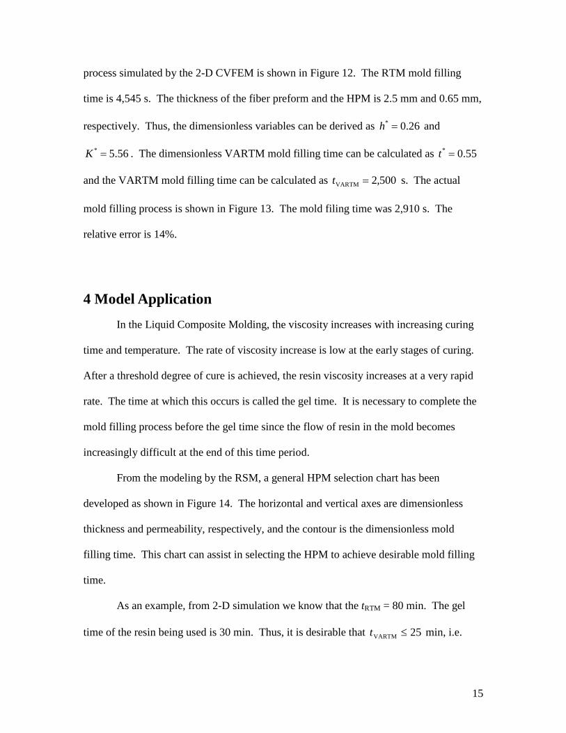
process simulated by the 2-D CVFEM is shown in Figure 12. The RTM mold filling

time is 4,545 s. The thickness of the fiber preform and the HPM is 2.5 mm and 0.65 mm,

respectively. Thus, the dimensionless variables can be derived as 26.0* =h and

56.5* =K . The dimensionless VARTM mold filling time can be calculated as 55.0* =t

and the VARTM mold filling time can be calculated as 500,2VARTM =t s. The actual

mold filling process is shown in Figure 13. The mold filing time was 2,910 s. The

relative error is 14%.

4 Model Application In the Liquid Composite Molding, the viscosity increases with increasing curing

time and temperature. The rate of viscosity increase is low at the early stages of curing.

After a threshold degree of cure is achieved, the resin viscosity increases at a very rapid

rate. The time at which this occurs is called the gel time. It is necessary to complete the

mold filling process before the gel time since the flow of resin in the mold becomes

increasingly difficult at the end of this time period.

From the modeling by the RSM, a general HPM selection chart has been

developed as shown in Figure 14. The horizontal and vertical axes are dimensionless

thickness and permeability, respectively, and the contour is the dimensionless mold

filling time. This chart can assist in selecting the HPM to achieve desirable mold filling

time.

As an example, from 2-D simulation we know that the tRTM = 80 min. The gel

time of the resin being used is 30 min. Thus, it is desirable that 25VARTM ≤t min, i.e.

16

31.0RTMVARTM* ≤= ttt .

Thus, the dimensionless thickness and permeability should be selected from the

shaded area shown in Figure 15. The corresponding thickness and permeability of the

HPM can be easily calculated.

5 Conclusions In this paper, a VARTM process model developed by 2-D CVFEM simulation,

the Design of Experiments, and the Response Surface Method (RSM) is presented. With

the permeability, porosity, and thickness of the fiber preform and the RTM mold filling

time as references, the dimensionless VARTM process variables and mold filling time

are introduced in this paper. The significant process variables were identified by using

the Design of Experiments (DOE). A quadratic regression model was developed by the

RSM. The model was validated against the 3-D VARTM simulation and experiments.

The results show that the accuracy is within 15% for most commonly used cases while

the computation time saving is over 99%. The approach presented in this paper provides

a general guideline for the VARTM process design and optimization. The process

variables and flow media can be quickly chosen by using the developed regression model,

which is extremely useful for composite part design in the early stage. It is also noticed

that for thick composite parts, this model yields a larger error because of the neglecting of

the through-thickness resin flow.

The advantages of this model are that the computation time is reduced

significantly. The complicated 3-D Finite Element modeling and material property

defining process are avoided, which makes this model very convenient for practical

17

applications. For example, the mold filling time can be obtained promptly when the

permeability and/or the thickness of the HPM have changed. The range for developing

the RSM based regression model have covered the normal application range. Thus, the

model is adequate in predicting the mold filling time of the VARTM process. The HPM

selection chart presented in this paper provides a convenient tool for flow media selection

and process optimization, which is extremely useful for composite part design in the early

stage.

The original contributions of this research are:

1. A guideline for VARTM process design is provided. The process parameters can

be selected per this guideline.

2. An efficient and effective approach is developed for the VARTM process

optimization. By using this approach, the process parameters can be found to

meet the objective in a time-efficient way.

3. Since variations exist for the process parameters, the approach presented in this

paper can also be used as a robust design tool to reduce the sensitivity to the

variations of process parameters.

References [1] Bruschke MV, Advani SG. Filling simulation of complex three-dimensional shell-

like structures. SAMPE Quarterly 1991; 23(1): 2-11.

[2] Young WB, Han K, Fong LH, Lee LJ. Flow simulation in molds with preplaced

fiber mats. Polymer Composites 1991; 12(6): 391-404.

18

[3] Liu XL. Isothermal flow simulation of liquid composite molding. Composites Part

A 2000; 31(12): 1295-1302.

[4] Lin RJ, Lee LJ, Liou MJ. Non-isothermal mold filling and curing simulation in

thin cavities with preplaced fiber mats, International Polymer Processing 1991;

VI(4): 356-369.

[5] Young WB. Three-dimensional nonisothermal mold filling simulation in resin

transfer molding. Polymer Composites 1994; 15(2): 118-127.

[6] Lee LJ, Young WB, Lin RJ. Mold filling and curing modeling of RTM and

SCRIM processes. Composite Structures 1994; 27(1-2): 109-120.

[7] Simacek P., Advani SG. Desirable features in mold filling simulations for liquid

molding processes. Polymer Composites (2004); 25(4): 355-367.

[8] Bruschke MV, Advani SG. A finite element/control volume approach to mold

filling in anisotropic porous media. Polymer Composites 1990; 11(6): 398-405.

[9] ESI Group. PAM-RTM. www.esi-group.com.

[10] Polyworx. www.polyworx.com.

[11] Mathur R, Heider D, Hoffmann C, Gillespie JW Jr., Advani SG, Fink BK. Flow

front measurements and model validation in the vacuum assisted resin transfer

molding process. Polymer Composites 2001; 22(4): 477-490.

[12] Loos AC, Sayre J, McGrane R, Grimsley B. VARTM process model development.

In: Proceedings of International SAMPE Symposium and Exhibition. Long Beach,

CA, May, 2001. 46(I): 1049-1061.

[13] Mohan RV, Shires DR, Tamma KK, Ngo ND. Flow channels/fiber impregnation

studies for the process modeling/analysis of complex engineering structures

19

manufactured by resin transfer molding. Polymer Composites 1998; 19(5): 527-

542.

[14] Sun XD, Li SJ, Lee LJ. Mold filling analysis in vacuum-assisted resin transfer

molding. part I: SCRIMP based on a high-permeable medium. Polymer

Composites 1998; 19(6): 807-817.

[15] Ni J, Li SJ, Sun XD, Lee LJ. Mold filling analysis in vacuum-assisted resin

transfer molding. Part II: SCRIMP based on grooves. Polymer Composites 1998;

19(6): 818-829.

[16] Tari MJ, Imbert JP, Lin MY, Lavine AS, Hahn HT. Analysis of resin transfer

molding with high permeability layers. Transactions of the ASME, Journal of

Manufacturing Science and Engineering 1998; 120(3): 609-616.

[17] Hsiao KT, Mathur R, Advani SG. A closed form solution for flow during the

vacuum assisted resin transfer molding process. Transactions of the ASME,

Journal of Manufacturing Science and Engineering 2000; 122(3): 463-475.

[18] Han K, Jiang SL, Zhang C, Wang B. Flow modeling and simulation of SCRIMP

for composite manufacturing. Composites Part A 2000; 31(1): 79-86.

[19] Dong CS. An equivalent medium method for the vacuum assisted resin transfer

molding process simulation. To appear in Journal of Composite Materials.

[20] Dong CS. Uncertainty analysis for fiber permeability measurement. Transactions

of the ASME, Journal of Manufacturing Science and Engineering 2005; 127(4).

[21] D’Arcy H. Les Fontaines Publiques de la villa de Dijon. Paris: Dalmont, 1856.

[22] Box GEP, Cox DR. An analysis of transformations, Journal of the Royal

Statistical Society, B 1964; 26: 211-243.

20

Figure 1: Vacuum assisted resin transfer molding process

Figure 2: Resin flow in VARTM process

21

Figure 3: 3-D anisotropy of composites

RTM

VARTM

Figure 4: RTM vs. VARTM mold filling

22

Part design (CAD) Material parameters (fiber, HPM) Processing parameters (viscosity, vacuum)

2-D RTM simulation

Dimensionless variables

VARTM process regression model

Dimensionless mold filling time

RTM mold filling time

VARTM mold filling time

Figure 5: Approach flowchart

Figure 6: Half normal plot, main effects and interaction plots

23

Thickness

Permeability

(0.40, 50.00)

(0.10, 10.00) (0.40, 10.00)

(0.10, 50.00)

(0.25, 30.00) (0.46, 30.00) (0.04, 30.00)

(0.25, 58.28)

(0.25, 1.72)

Figure 7: Central Composite Design (CCD)

Figure 8: Response surface of the fitted regression model

Figure 9: A boat hull

24

(a) Mesh (b) Resin flow

Figure 10: RTM boat hull processing

a) Mesh b) Resin flow

Figure 11: VARTM boat hull processing

Figure 12: RTM simulation of car hood

25

Figure 13: VARTM processing of car hood

Figure 14: General HPM selection chart

26

Figure 15: Example of HPM selection

27

Table 1: Mold filling simulation of RTM and VARTM processes

Permeability (darcy) Mold filling time (s) VARTM-RTM mold filling time ratio K11f K11H RTM VARTM

Linear 50 1500 98.90 16.80 0.170 100 3000 49.50 8.41 0.170 200 6000 24.70 4.20 0.170 Port 50 1500 343.00 66.00 0.192 100 3000 171.00 33.00 0.193 200 6000 85.70 16.50 0.193

Table 2: Level selection

Low High Low High hH (mm) 0.4 1.6 h* 0.1 0.4 φH 0.7 0.9 φ* 1.4 1.8 KH (darcy) 1,000 5,000 K* 10 50