1

Development of a Pressure-Based CFD Solver for All-Speed Flows on Arbitrary Polygonal Meshes in a Rule-Based Framework

Thermal and Fluids Analysis Workshop (TFAWSO3), Aug. 18-22, Hampton, VA

Jeffrey Wright 1,2 and Siddharth Thakur 1,2

1 Streamline Numerics, Inc., Gainesville, Florida (UF)

2 Dept. of Mechanical & Aerospace Engg., University of Florida ______________________________________________________________________________ 1. INTRODUCTION

Over the last decade significant new technologies have been developed which allow the

scientist/engineer to design reliable programs for simulating the complex physics involved in turbulent flow combustion devices. In the area of numerical algorithm development, a significant step forward has come with the maturation of unstructured grid methods, which provide a host of benefits over traditional methods employing structured multi-block grids with a curvilinear coordinate framework. Some of these benefits, which have been extensively discussed in the literature, include the ease of mesh generation, mesh refinement and mesh movement for problems with moving domain boundaries. One of the most practical benefits, though, is the ease with which numerical algorithms can be developed for the automatic mapping of unstructured grids to parallel, distributed-memory computer architectures, which are evolving as the architectures of choice for computer codes which are being employed to solve problems of ever-increasing complexity, involving multi-disciplinary physics and ever-increasing grid size. There are, however, some disadvantages associated with unstructured grid methods, primarily in the form of increased data file size and program memory compared to structured grid counterparts, as well as the extra challenge required to obtain optimum performance of unstructured codes on cache-based memory architectures. However, with advances in computer hardware, these do not appear to be stumbling blocks.

In addition to numerical algorithm development, great strides have been made in the area of

program development tools. The most notable of these advances has been the proliferation of object-oriented programming methods, of which, C++ seems to be gaining popular favor in the scientific and engineering communities. Sometimes overlooked in importance relative to both physical and numerical modeling as only a means to an end, the use of object-oriented methods for program design can significantly enhance the overall process by allowing developers to concentrate more on physical models and advanced numerical techniques rather than the actual mechanics of writing and maintaining code. Some adjustment is required, however, when moving from traditional procedural-based languages such as FORTRAN90 to object-oriented languages. Object- oriented languages, C++ in particular, provide a much wider programming vocabulary, allowing developers to write code which expresses the overall design in a more conceptual way than can be obtained with procedural languages. This vocabulary, however, can easily be misused with disastrous results, if care is not taken, resulting in codes which run significantly slower than their FORTRAN90 counterparts. With proper use, though, this does not have to be the case.

2

Recently, a new framework for application development called LOCI (Ref. [5]) has been

developed at the Mississippi State University. LOCI is designed to reduce the complexity of assembling large-scale finite-volume applications as well as the integration of multiple applications in a multidisciplinary environment. LOCI utilizes a rule-based framework for application design, and is an interesting alternative to the use of object-oriented design in C++. Users of LOCI write applications using a collection of “rules” and provide an implementation for each of the rules in the form of a C++ class. In addition, the user must create a database of “facts” which describe the particular knowns of the problem, such as boundary conditions. Once the rules and facts are provided, a query is made to have the system construct a solution. One of the interesting features of LOCI is its ability to automatically determine the scheduling of events of the program to produce the answer to the desired query, as well as to test the consistency of the input to determine whether a solution is possible given the specified information. The other major advantage of LOCI to the application developer is its automatic handling of domain decomposition and distribution of the problem to multiple processors. This feature alone makes LOCI a very attractive alternative as it allows scientists/engineers who have neither the time, the training, nor the inclination to understand the intricacies of message passing (e.g. MPI) to write code for distributed memory platforms.

The algorithms for the solution of Reynolds-averaged Navier-Stokes (RANS) equations can be

broadly classified as: (a) pressure-based and (b) density-based methods. Examples of the former are the structured grid-based STREAM [Ref. 1] code and the unstructured grid-based STREAM-UNS code [Ref. 2,3]. An example of a density-based code is the CHEM [Ref. 4] code which uses the LOCI framework. Both density-based and pressure-based methods have their advantages and disadvantages which have been well documented in the literature. Density-based methods are typically most efficient and robust at the higher-end of the Mach number spectrum and the pressure-based methods at the lower-end of the spectrum. Used in conjunction, they can compliment each other to yield an optimum performance for all-speed flows which are the norm in propulsion devices. Thus, it is desirable to develop a computational tool that utilizes both these methods in a single framework. The framework chosen for this is LOCI.

In this paper, we will discuss various issues involved in implementing the technology from a

currently existing FORTRAN90 code called STREAM into a new code called STREAM-UNS-LOCI programmed in the LOCI framework. STREAM is a pressure-based, multi-block, Reynolds-averaged Navier-Stokes (RANS) code, which has been extensively developed and tested over the last decade. The code is designed to handle all-speed flows (incompressible to supersonic) and is particularly suitable for solving multi-species flow in fixed-frame combustion devices, as well as turbomachines with multiple stationary and rotating components. In the following sections, we first present the salient features of STREAM and then discuss some of the advantages/disadvantages that are to be gained in moving to the unstructured grid environment. Finally, we discuss the rule-based LOCI system and compare/contrast this approach with that of traditional object-oriented design. 2. PRESSURE-BASED METHODOLOGY: STREAM

STREAM is a pressure-based flow solver (Ref. [1]) which employs structured body-fitted grids

for computing steady compressible and incompressible, laminar and turbulent flows. For handling

3

complex geometries, multiblock abutting grids with flux conservation at the block interfaces, are employed. Various convection schemes including first-order upwind, second-order upwind, central difference and QUICK are available in STREAM.

The flow solver is based on the SIMPLE (Semi-Implicit Method for Pressure-Linked

Equations) algorithm (Ref. [7]). It uses a control volume approach with a collocated arrangement for the velocity components and the scalar variables like pressure. Pressure-velocity decoupling is prevented by employing the momentum interpolation approach (Ref. [8]); this involves adding a fourth-order pressure dissipation term while estimating the mass flux at the control volume interfaces. The velocity components are computed from the respective momentum equations. The velocity and the pressure fields are corrected using a pressure correction ( p′ ) equation. The correction procedure leads to a continuity-satisfying velocity field. The whole process is repeated until the desired convergence is reached. The details of the implementation of STREAM can be found in Ref. [1].

2.1. Governing Equations The governing equations that are used are the equations of mass continuity, momentum, energy

and species transport:

( ) 0jj

ut xρ ρ∂ ∂+ =

∂ ∂ (1)

( ) ( ) jii j i

j i j

pu u ut x x x

τρ ρ

∂∂ ∂ ∂+ = − +

∂ ∂ ∂ ∂ (2)

( ) ( ) ( )jj i ij

j j j

q pH u H ut x x x tρ ρ τ

∂∂ ∂ ∂ ∂+ = − + +

∂ ∂ ∂ ∂ ∂ (3)

( ) ( ) , 1,ii j i

j j j

YY u Y i NSt x x xρ ρ µ ω

• ∂∂ ∂ ∂+ = + = ∂ ∂ ∂ ∂

(4)

where ρ is density, iu is velocity vector, p is pressure, iY is the mass fraction of species i (out of a total of NS species), ijτ is viscous stress tensor, jq is heat flux vector; H is the total (or stagnation) enthalpy given by

12 i iH h u u= + (5)

with h being the specific enthalpy which is related to the temperature (T) as

( )0

0

T

i piTh h C dT= +∑ ∫ (6)

where piC is the specific-heat (for constant pressure processes) for the ith species. An equation of state is required to relate the density to the thermodynamic variables; for an ideal gas, we use the following: p RTρ= (7) where R is the gas constant.

The constitutive relation between stress and strain rate for a Newtonian fluid is used to relate the components of the stress tensor to velocity gradients:

4

( ) 2 23 3

ji lij t ij ij

j i l

uu u kx x x

τ µ µ δ ρ δ ∂∂ ∂

= + + − ⋅ − ∂ ∂ ∂ (8)

where µ is the molecular viscosity and tµ is the turbulent (eddy) viscosity to be defined later. The heat flux vector is obtained from Fourier’s law:

Pr

tj

t j

Tqx

µκ ∂

= − + ∂ (9)

where ijδ is the Kronecker delta and κ is the thermal conductivity; LPr is the laminar Prandtl number defined as:

Pr pL

C µκ

= (10)

For turbulence closure, the model employed is the k-ε model. The eddy viscosity is estimated from the turbulent kinetic energy (k) and the rate of dissipation of turbulent kinetic energy (ε) by the following relationship:

2

t

C f kµ µ ρµε

= (11)

The k and ε are estimated by their own transport equations which can be written, in Cartesian coordinates, as the following:

( ) ( ) ti k

i i k i

kk u k Pt x x x

µρ ρ µ ρε

σ ∂ ∂ ∂ ∂

+ = + + − ∂ ∂ ∂ ∂ (12)

( ) ( )2

1 2t

i ki i i

u C P Ct x x x k kε

µ ε ε ερε ρ ε µ ρσ

∂ ∂ ∂ ∂+ = + + − ∂ ∂ ∂ ∂

(13)

where kP is the production of k from the mean flow shear stresses and is given by

ji i ik ij t

j j i j

uu u uPx x x x

τ µ ∂∂ ∂ ∂

= = + ⋅ ∂ ∂ ∂ ∂ (14)

The term ω represents the chemical heat release source terms which are obtained from the laws of mass action. A set of chemical reactions can be expressed as follows for the ith species of the jth reaction, in terms of the stoichiometric coefficients ( ijν ′ and ijν ′′ for the reactants and products, respectively):

1 1

, 1,...,f j

b j

NS NSK

ij i ij iKi i

M M j NRν ν= =

→′ ′′ =←∑ ∑ (15)

The net rate of change of the molar concentration, ijX , of species i due to reactions j is given by

( )ij ij

j j

i iij ij ij f b

i iWi Wi

Y YX K KM M

ν νρ ρν ν

′ ′′ ′′ ′ = − −

∏ ∏ (16)

and the net species production rate, iω , is obtained by summing over all reactions:

1

NR

i Wi ijj

M Xω=

= ∑ (17)

The forward rate of reaction is given by the modified Arrhenius law:

5

expj

j

B jf j

EK A T

RT

= −

(18)

and the corresponding backward reaction can be obtained from

j

j

j

fb

eq

KK

K= (19)

where jeqK is the equilibrium coefficient given by

( )

1

0

.expj

j

NS

j j ii

eq

GRTKp RT

ν ν ν∆

=

′′ ′− = −

∑ (20)

where iG is the Gibb’s free energy and

1 1

NS NS

j ij iji i

ν ν ν= =

′ ′′∆ = −∑ ∑ (21)

In the above equations, jA , jB and jE are constants.

2.1. Transformation to Curvilinear Coordinates

For arbitrary shaped geometries, the governing equations are transformed into generalized curvilinear coordinates (ξ, η, ζ), where ξ=ξ(x,y,z), η=η(x,y,z) and ζ=ζ(x,y,z). The transformation of the physical domain (x,y,z) to the computational domain (ξ,η,ζ) is achieved by the following relations:

11 12 13

21 22 23

31 32 33

1x y z

x y z

x y z

f f ff f f

Jf f f

ξ ξ ξη η ηζ ζ ζ

=

(22)

where the metrics are

11 12 13, ,f y z z y f z x x z f x y y xη ζ η ζ η ζ η ζ η ζ η ζ= − = − = − 12 22 23, ,f z y y z f x z z x f y x x yξ ζ ξ ζ ξ ζ ξ ζ ξ ζ ξ ζ= − = − = − (23) 31 32 33, ,f y z z y f z x x z f x y y xξ η ξ η ξ η ξ η ξ η ξ η= − = − = − and J is the Jacobian determinant of the transformation given by

( , , )( , , )

x x xx y zJ y y y

z z z

ξ η ζ

ξ η ζ

ξ η ζ

ξ η ζ∂

= =∂

(24)

6

Figure 1. 2-D structured grid (a) Physical plane. (b) Transformed (computational) plane.

2.3. SIMPLE Algorithm for Pressure-Velocity Coupling Following the standard procedure employed in the SIMPLE algorithm (Ref. [7]), suppose that

the velocity field at an intermediate step of the iterative solution procedure is given by u*, v* and w*, corresponding to a pressure field p*. The new predicted velocity and pressure fields can then be obtained by adding a correction as follows: * * * *, , ,p p p u u u v v v w w w′ ′ ′ ′= + = + = + = + (25)

To obtain the pressure and velocity corrections, first the u-momentum equation for this intermediate velocity field is written as * * *u

P P nbr nbr P D CA u A u S S S= ∑ ⋅ + + + (26) where ( )* * * *

11 21 31PS f p f p f pξ η ζ= − + + (27) From this, an expression for the correction of the u-component of velocity can be obtained:

( )11 21 311

uP

u f p f p f pA ξ η ζ′ ′ ′ ′= − + + (28)

Similarly, v′ and w′ can be written as functions of p′ . Finally, plugging the predicted velocity field ( *u u u′= + , etc.) into the continuity equation yields an equation for p′ :

( ) ( )1 nnvp V p C p V

RT t RT tρρ ρ

′ ∆ ′ ′+ ∇ −∇ ∇ = − −∇ ∆ ∆ i i i (29)

where the superscript n represents solution at the old time level.

2.4. PISO-Based Predictor-Corrector Algorithm for Unsteady Flows The steady-state SIMPLE algorithm can be extended in a straightforward manner for unsteady

flows by including the unsteady terms in the Navier-Stokes equations. However, this approach is computationally expensive since several iterations have to be conducted at each timestep. A more

(i,j) •(i-1,j)

•

(i-1,j-1) • • (i,j-1)

7

efficient procedure has been developed in Ref. [9] which is based on the PISO algorithm of Ref. [10]. The unsteady algorithm can be summarized as follows: • Start with the previous timestep values: , , , ,n n n n nu v p Tρ • Predictor: solve the momentum equations implicitly treating the pressure gradient from the

previous timestep explicitly to get *u and *v • First corrector:

Compute control volume interface velocities Compute p′ and update velocities using p′ to get **u and **v Update pressure using p′ and density from equation of state to yield *p and *ρ

• Second corrector Compute p′′ Update velocities using p′′ to get ***u and ***v Update pressure and density to obtain **p and **ρ from equation of state

***u , ***v , **p , **ρ are considered the values at the new time level (n+1) and we proceed to the first step above for the next time level.

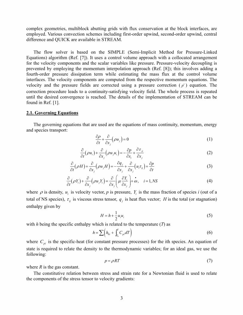
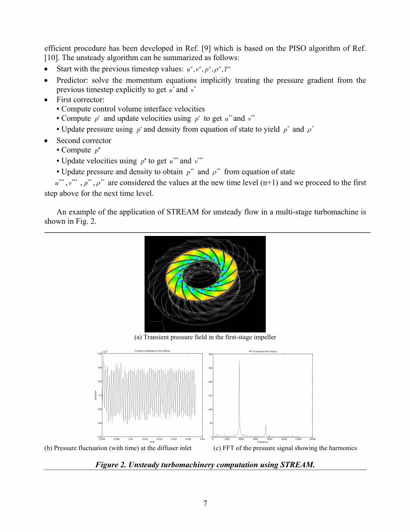
An example of the application of STREAM for unsteady flow in a multi-stage turbomachine is

shown in Fig. 2.

(a) Transient pressure field in the first-stage impeller

(b) Pressure fluctuation (with time) at the diffuser inlet (c) FFT of the pressure signal showing the harmonics

Figure 2. Unsteady turbomachinery computation using STREAM.

0 2000 4000 6000 8000 10000 12000 140000

50

100

150

200

250

300FFT of pressure time history

Frequency0.006 0.008 0.01 0.012 0.014 0.016 0.018 0.02

7.54

7.56

7.58

7.6

7.62

7.64

7.66x 10

4

pre

ssure

time

Pressure Oscillations in the Diffuser

8

3. FROM STRUCTURED (STREAM) TO UNSTRUCTURED (STREAM-UNS)

In writing finite volume applications within the structured curvilinear-coordinate framework, a number of complexities appear which are simply a result of use of this framework. These issues can be categorized as follows:

1) Curvilinear coordinate framework issues. 2) Multi-block framework issues.

In the early development of structured grid algorithms for grid generation and finite-volume Navier-Stokes solvers, curvilinear coordinates were adopted as a natural way to map physical space to computational space. While this mapping initially appears convenient, it introduces quite a lot of unnecessary difficulty into the process of finite-volume discrete integration. The primary source of excess complexity arises with terms in the governing equations which contain products of derivatives, such as the viscous dissipation term of the energy equation. This term can be naturally expanded in the form of Cartesian gradients. When using curvilinear coordinates each of the Cartesian gradients is expanded into gradients in computational space along with corresponding metrics. Such an expansion immediately triples the number of terms in the equation. In the process of unstructured grid assembly, curvilinear coordinates are completely abandoned and the Cartesian gradient components are evaluated directly with the aid of the relation derived from the divergence theorem

Another major complexity introduced via curvilinear coordinates is the artificial separation of control volume faces into three distinct types. These are commonly labeled as North, South, East, West, Top and Bottom faces as shown in Fig. 1. The typical assembly for a scalar convection/diffusion/source equation involves an internal loop over the interior control volumes of a block to compute fluxes. Separate loops are then undertaken to handle boundaries. Since the boundaries fall along three different computational space coordinate surfaces, three distinct loops are required to complete the assembly process. In the process of unstructured grid finite volume integration, all modern solvers now use the process of either face-based or edge-based assembly. In this process, fluxes for each of the control volumes is assembled by a sweep over the faces (when variables are cell-centered) or edges (when variable are node- centered) of the grid. Taking the face-based process for example, the only distinction now made during flux assembly is between an interior face and a boundary face. Interior faces are those which contain elements on both sides and boundary faces those which are connected to a single element. This type of assembly process has been found to greatly reduce the amount of code required. In addition to theses complexities, the multi-block framework in itself leads to several algorithmic complications which disappear when employing unstructured grids. Since the complete domain is decomposed into a number of blocks, an entirely separate set of functions must be employed to communicate information between these blocks. For general block-to-block connectivities, these functions can become quite complex, especially if one-to-one connectivity (grid points match at the boundary between blocks) is not present. Since the unstructured grid contains no blocks, this additional complexity does not arise.

The multi-block approach also creates complications regarding domain decomposition. Since multi-block codes are most naturally decomposed into functions which operate on individual blocks, the desire to maintain this structure often means that domain decomposition is performed at the block level as well. Such a choice often leads to load-balancing problems in the distributed memory environment, in which each processor is performing calculations on a single block of the

9

domain. To achieve equal load balancing, in which all processors have an equal amount of work, in some instances, structured multi-block codes require all blocks to have the same number of grid points, which while alleviating the load-balancing problem, can result in excessive grid generation time and an overall waste of grid points. With the unstructured grid approach, sophisticated automatic domain decomposition methods such as METIS [Ref. 11] have been developed which eliminate these problems and result in a good level of load balancing for general unstructured grids.

While the benefits of migrating to unstructured grids are clear, the structured grid framework does provide one advantage. Overlooking the code complexity issue, once a structured code is written and well-tested, these codes tend to give generally higher performance than unstructured codes on cache-based memory architectures, since memory is accessed in a more uniform manner. This is entirely attributable to the ordered nature of the arrays used in structured codes. To use cache-base memory machines in an efficient manner, unstructured codes must employ node/edge/element reordering functions to ensure efficient memory access. Even with these considerations, structured grid codes are still superior in this regard.

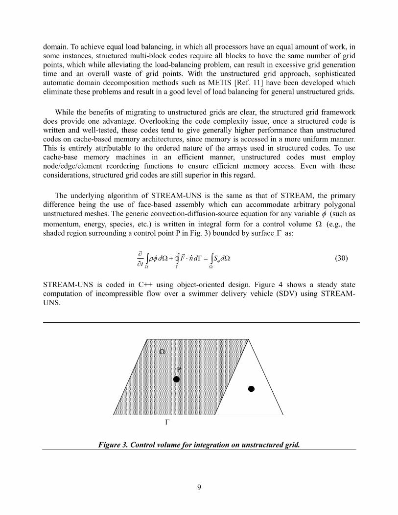
The underlying algorithm of STREAM-UNS is the same as that of STREAM, the primary

difference being the use of face-based assembly which can accommodate arbitrary polygonal unstructured meshes. The generic convection-diffusion-source equation for any variable φ (such as momentum, energy, species, etc.) is written in integral form for a control volume Ω (e.g., the shaded region surrounding a control point P in Fig. 3) bounded by surface Γ as:

ˆd F n d S dt ϕρφΩ Γ Ω

∂Ω + ⋅ Γ = Ω

∂ ∫ ∫ ∫ (30)

STREAM-UNS is coded in C++ using object-oriented design. Figure 4 shows a steady state computation of incompressible flow over a swimmer delivery vehicle (SDV) using STREAM-UNS.

Figure 3. Control volume for integration on unstructured grid.

P

Γ

Ω

10

Figure 4. Submerged vehicle computation using STREAM-UNS.

4. RULE-BASED FRAMEWORK: STREAM-UNS-LOCI

In this section we provide a basic overview of the LOCI programming system (Ref. [5]) and

describe how it can be used to implement unstructured grid solvers. For more complete details on the LOCI system, the reader should consult the LOCI tutorial (Ref. [6]) which is available with the LOCI distribution. Following this overview, we will discuss some of the anticipated benefits of using LOCI and outline the strategy for testing the feasibility of using LOCI for pressure-based unstructured grid assembly.

4.1. LOCI: Overview Programs written using LOCI consist of the following three general components:

1) Fact Database: This database which is maintained by LOCI contains all information which is known about the problem being solved. For finite-volume programs for fluid-flow and heat transfer, this information usually consists of items such as boundary conditions, initial conditions, material properties, and the combustion mechanism among other things. The fact database is usually constructed during the input section of the user's program. For example, the user may have a function called readBoundaryConditions() inside which the boundary conditions associated with the problem would be read and entered into the fact database. 2) Rules: Rules can be thought of as the components of the finite-volume algorithm which are used to compute the desired solution from the known facts. Each rule can be represented in symbolic form by a “rule signature”. For example, a rule to compute the centroid of the triangles in a 2-D unstructured grid can be represented by the following rule signature:

triangleCentroid<-triangleNodes->position This rule can be translated as “the centriod of each triangle is computed from the position property of the triangle's nodes”. The “<-” operator signifies the output of a rule, while the “->” operator

11

signifies that we are using the position property of the triangle nodes in the calculation process. This rule signature is really only a symbolic representation of what the rule is doing. For each rule signature, the programmer must supply a C++ class which actually implements the functions of the rule. An example of this will be given in a later section. 3) Query: Once the facts and rules are specified, one obtains the solution by executing a “query” to the fact database for a desired solution. At this point LOCI attempts to order all the rules into an execution schedule which can produce the solution. If LOCI finds that it is not possible to arrive at a solution given the known facts and list of rules, it will inform the user.

For completeness, a skeleton main function for a finite volume code is shown in Fig. 5. int main(int argc,char *argv[]) // Initialize the LOCI system. Loci::Init(&argc,&argv) ; // Setup the fact database and read known facts. Grid and boundary conditions // are inserted into the fact database. fact_db factDatabase ; readGrid(factDatabase) ; readBoundaryConditions(factDatabase) ; ... // Add all previously registered rules which define the finite-volume // program to the rule database. Each rule is specified as a C++ class and // registered in the global rule list in a separate implementation file. rule_db ruleDatabase ; ruleDatabase.add_rules(global_rule_list) ; // Distribute the rules and facts to the various processors. int numProcesses=Loci::MPI_processes,myID=Loci::MPI_rank ; std::vector<entitySet> partition=Loci::generate_distribution (factDatabase,ruleDatabase) ; Loci::distribute_facts(partition,factDatabase,ruleDatabase) ; // Specify the 'query' and set up an execution schedule to satisfy it. Here // we are asking for the solution, which also happens to be a rule. string query("solution") ; executeP schedule=create_execution_shedule(ruleDatabase,factDatabase,query) ; // Execute the schedule to produce the solution. schedule->execute(factDatabase) ; // Finalize the LOCI system. Loci::Finalize() ;

Figure 5. LOCI: Example 1.

4.2. Basic Data Structures of LOCI

In order to provide some foundation for understanding the implementation files for the rules which compose any finite-volume program constructed using the LOCI system, we present some of

12

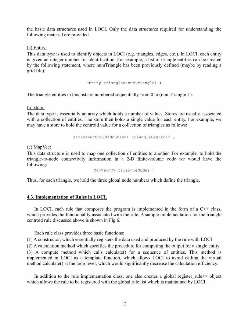
the basic data structures used in LOCI. Only the data structures required for understanding the following material are provided. (a) Entity: This data type is used to identify objects in LOCI (e.g. triangles, edges, etc.). In LOCI, each entity is given an integer number for identification. For example, a list of triangle entities can be created by the following statement, where numTriangle has been previously defined (maybe by reading a grid file):

Entity triangles(numTriangle) ; The triangle entities in this list are numbered sequentially from 0 to (numTriangle-1). (b) store: The data type is essentially an array which holds a number of values. Stores are usually associated with a collection of entities. The store then holds a single value for each entity. For example, we may have a store to hold the centroid value for a collection of triangles as follows:

store<vector2d<double>> triangleCentroid ;

(c) MapVec: This data structure is used to map one collection of entities to another. For example, to hold the triangle-to-node connectivity information in a 2-D finite-volume code we would have the following:

MapVec<3> triangleNodes ;

Thus, for each triangle, we hold the three global node numbers which define the triangle.

4.3. Implementation of Rules in LOCI. In LOCI, each rule that composes the program is implemented in the form of a C++ class,

which provides the functionality associated with the rule. A sample implementation for the triangle centroid rule discussed above is shown in Fig 6.

Each rule class provides three basic functions:

(1) A constructor, which essentially registers the data used and produced by the rule with LOCI (2) A calculation method which specifies the procedure for computing the output for a single entity. (3) A compute method which calls calculate() for a sequence of entities. This method is implemented in LOCI as a template function, which allows LOCI to avoid calling the virtual method calculate() at the loop level, which would significantly decrease the calculation efficiency.

In addition to the rule implementation class, one also creates a global register_rule<> object which allows the rule to be registered with the global rule list which is maintained by LOCI.

13

class triangleCentroid : public pointwise_rule private: const_store<vector2d<double> > position ; const_MapVec<3> triangleNodes ; store<vector2d<double> triangleCentroid ; public: // Constructor to provide symbolic names for the data used in // this rule and to define the input and output quantities. triangleCentroid() name_store("position",position) ; name_store("triangleNodes",triangleNodes) ; name_store("triangleCentroid",triangleCentroid) ; input("triangleNodes->position") ; output("triangleCentroid") ; // Method which performs the calculation for a single Entity. void calculate(Entity e) triangleCentroid[e]=(position[triangleNodes[e][0]]+ position[triangleNodes[e][1]]+position[triangleNodes[e][2]])/3.0 ; // Template function to call the calculate method for a sequence of // entities. virtual void compute(const sequence &sequence) do_loop(sequence,this) ; ; // Create a global object that will register this rule in the global // rule list. register_rule<triangleCentroid> registerTriangleCentroid ;

Figure 6. LOCI: Example 2.

4.4. Benefits of Using the LOCI Framework In using any new system for writing finite-volume applications, the general hope is that one

will spend less time on the actual mechanics of writing code, and thus more time concentrating on improving other aspects of the solver, such as the implementation of additional turbulence models or the integration with other solvers to handle multi-disciplinary physics. After all, scientists/ engineers are not in the business of writing code for fun usually there is a physical problem that needs to be solved. In this regard, there are two major benefits which are envisioned in using LOCI, rather than other modern coding techniques such as standard object-oriented programming in C++.

(a) LOCI is designed with multi-disciplinary problems in mind. (b) LOCI automatically handles the partitioning of the unstructured problem in the distributed-memory environment.

14

(a) Seamless Integration of Multi-Disciplinary Physics With the rapid development of computer hardware, it is now feasible to solve quite complex

problems involving multi-disciplinary physics. For example, one may solve a fluid flow/heat transfer problem in some combustion device, where one not only computes the fluid flow using a finite-volume solver, but also solves the heat-transfer and stress problem in the solid section of the device simultaneously. One approach commonly used these days is to solve each section (fluid or solid) independently and iterate several times until a converged solution is obtained in both regions. In this approach, the fluid and solid solution procedures are said to be loosely coupled, and in fact most often are obtained using different solvers which known nothing of the other. This approach works, but is usually a very slow process due to the loose nature of the coupling between the two domains.

A better approach to the multidisciplinary problem involves the so-called tight coupling

between the components, in which the different solvers operate in a more closely coordinated manner. In such a fashion, each of the solvers has some knowledge of the other, and the interface between the components allows data to be exchanged at a much higher frequency, usually at the inner iteration level. In the most extreme case of tight coupling, all components (fluid/heat- transfer/stress) are solved together simultaneously at every iteration. In this case, there is really only one solver.

One of the major strengths of LOCI is its ability to handle all approaches, from loosely-coupled

to tightly-coupled. When writing applications in LOCI, it is not necessary that all components of the application be entirely written within the rule-based framework. Applications can exist as independent modular components which can be linked to other components written entirely in LOCI by encapsulating the component as a rule. For example, LOCI has an interface to the PETSc [Ref. 12] linear algebra library. In both the loosely- and tightly-coupled approaches, a significant advantage of LOCI is its ability to check the internal consistency of a program. Often times, components of a multidisciplinary application may be written by different developers, who may not have detailed knowledge of all system components. When all components are used to solve a given problem, LOCI guarantees that a program schedule is generated which ensures that information between the components is computed at the appropriate time and all information required by each component is available when it is needed. If the components cannot be linked together due to an insufficient specification of the interface between them, LOCI informs the user that a schedule cannot be generated and terminates execution. This feature completely eliminates errors associated with inter-component coordination, which become more common in complex codes written in a multidisciplinary environment.

(b) Grid Partitioning for Distributed-Memory Environment

Regarding the second issue, one can see from the main program example in Fig. 5 that it is very

simple to create programs which can run in a distributed memory environment. LOCI handles all partitioning of the problem, including the grid, the rule database and the fact database. This feature of LOCI is a major advantage over other approaches such as standard object-oriented C++, where the programmer must entirely code and debug a separate layer of the program devoted to

15

partitioning of the problem. For scientists/engineers inexperienced in the area of message-passing (e.g. MPI), the use of LOCI can entirely eliminate the need for this extra complexity.

4.6. Plan for Implementation and Testing of STREAM-UNS-LOCI

The primary criteria for judging the effectiveness of LOCI lies in answering the following questions: (1) Is there a significant advantage to be gained in program organization and simplification by using LOCI, in comparison with standard object-oriented C++? (2) The internals of LOCI are a black box to the programmer. So, are the resulting programs as efficient as the currently-existing version STREAM-UNS which employs standard object-oriented techniques in C++?

In order to answer these questions, the technology of STREAM-UNS will be ported to a new code called STREAM-UNS-LOCI written entirely in the LOCI framework. This new code will be tested versus existing implementations of STREAM-UNS written using standard object-oriented techniques in C++, with standard MPI message passing for the distributed computing environment. Regarding code organization and maintenance, we have found that object-oriented techniques significantly improve both the initial program design as well as the ability to enhance and maintain codes as new features are added. Whether the use of a rule-based (as opposed to object-based) system improves one's ability to develop and maintain code can only be answered by a direct head-to-head comparison. In addition, since all data is allocated and controlled by the LOCI system, the programmer has less control of the internal representation of the data. In traditional object-oriented approaches, especially for codes finely tailored to a specific application (e.g. fluid flow solvers) concrete data types are created which have a very narrow scope of function, but are therefore highly efficient. Will the more general data types provided by LOCI achieve the same level of performance? Results of this ongoing work will be reported at a later date in hopes that a better understanding of LOCI in relation to its application to pressure-based solvers can assist others in deciding if LOCI is a viable alternative to the more traditional approaches for program development. REFERENCES 1. Thakur, S, Wright, J. and Shyy, W., “STREAM: A Computational Fluid Dynamics and Heat Transfer

Code for Complex Geometries. Part 1: Theory. Part 2: User Guide,” Streamline Numerics, Inc. and University of Florida, Gainesville, Florida (1999).

2. Wright, J. and Smith, R., “An Edge-Based Method for the Incompressible Navier-Stokes Equations on

Polygonal Meshes,” Journal of Computational Physics, Vol. 169, No. 1, pp 24-43 (2001). 3. Wright, J., “STREAM-UNS: A 3-D Pressure-Based Navier-Stokes Flow Solver for Unstructured

Grids,” Streamline Numerics, Gainesville, Florida (2002). 4. Luke, E.A., “CHEM: A Finite-Rate Inviscid Chemistry Solver – the User Guide,” Mississippi State

University (1999).

16

5. Luke, E.A., “LOCI: A Deductive Framework for Graph-Based Algorithms,” Third International Symposium on Computing in Object-Oriented Parallel Environments, edited by S. Matsuoka, R. Oldehoeft and M. Tholburn, No. 1732 in Lecture Notes in Computer Science, Springer-Verlag, pp 142-153 (Dec. 1999).

6. Luke, E.A., “Loci: A Tutorial,” Mississippi State University (2002). 7. Patankar, S.V., Numerical Heat Transfer and Fluid Flow, Hemisphere, Washington, D.C.

(1980). 8. Rhie, C. L. and Chow, W. L., “A Numerical Study of the Turbulent Flow Past an Isolated

Airfoil with Trailing Edge Separation,” AIAA J., Vol. 21, pp1525-1532 (1983). 9. Thakur, S and Wright, J. 2003, “An Operator-Splitting Algorithm for Unsteady Flows at All

Speeds in Complex Geometries,” to appear. 10. Issa, R.I 1986, “Solution of Implicitly Discretized Fluid Flow Equations by Operator Splitting,”

J. Comp. Physics, Vol. 62, pp 40-65. 11. Karypis, G. and Kumar, V., “A Fast and High Quality Multilevel Scheme for Partitioning

Irregular Graphs,” SIAM J. of Scientific Computing, 1998. 12. Balay, S., Buschelman, K., Gropp, W., Kaushik, D., Knepley, M., McInnes, L., Smith B. and

Zhang, H., “PETSc User’s Manual,” Argonne National Laboratory Report, ANL-95/11-Revision 2.1.5 (2003).