Special Publication SJ99-SP3

FINAL REPORT

DEVELOPMENT OF A POPULATION-BASED WATER USE MODEL

Submitted To The St. Johns River Water Management District

CONTRACT NO. 96H200

GeoFocus, Inc.1155 NW 13th Street

Gainesville, Florida 32601

Principal Investigator

Richard L. DotyJune 16,1998

EXECUTIVE SUMMARY

The population-based water use model was developed for the St. Johns RiverWater Management District (District) to help plan for future water demand. Thisraster GIS-based model distributes the county population projections of the Bureauof Economic and Business Research into square mile sections. It does this bycalculating a weighted average of the growth rate (from 1981 through 1990) of eachsection, and factoring in the positive influence of spatial features such as roads,water bodies, and existing residential and commercial areas. It then excludes non-developable lands, including wetlands, conservation areas, inappropriate land uses,road rights-of-way, and areas that have already reached their maximum allowabledensity, or are "built out". The remaining areas are then allocated populationgrowth by section according to the section's growth rate and proximity to spatialinfluences. This growth by section is then summarized by utility service areaboundaries for comparison with utility and local government estimates.

The model was run on all 19 counties within the District, but Orange Countywas selected as the prototype to be analyzed in this report because of that county'slarge population and rapid growth. The results of a comparison to transportationanalysis zone (TAZ)-based models are also discussed in this report.

CONTENTS

EXECUTIVE SUMMARY i

CONTENTS ii

FIGURES iii

TABLES iv

APPENDICES v

INTRODUCTION 1Overview of Project Requirements 1Overview of Historical Population Trends 1The Impetus for Modeling Population Growth 2Overview of Geographic Information Systems (GIS) 2

MODEL METHODOLOGY 5Historical Element Overview 5Historical Element 8Maximum Density Determination 12Spatial Element 12Growth Suitability Grid 14Distribution of Growth by Section 14Updates in Model Inputs from Prior Model Periods 15Final Output of Model 15Utility Service Area Growth Summary Grids 16

CONCLUSION AND DISCUSSIONFinal Output of Model. 23Future Improvements to the Model 24The Future of Growth Modeling and GIS 26

REFERENCE LIST 27

FIGURES

The Modeling Process for Predicting the Spatial Distribution ofFuture Population Growth for the St. Johns River WaterManagement District 6

in

TABLES

1 Data Layers in Exclusionary Mask Grid 13

2 Data Layers in Growth Influence Surface 13

3 District Model Results for Orange County by Utility ServiceArea 18

4 District Model Results for Volusia County by Utility ServiceArea 18

5 TAZ-Based Model Results for Orange County by Utility ServiceArea 19

6 TAZ-Based Model Results for Volusia County by Utility ServiceArea 19

7 Differences Between District Model Results and TAZ-BasedModel Results for Orange County by Utility Service Area 20

8 Differences Between District Model Results and TAZ-BasedModel Results for Volusia County by Utility Service Area 20

9 Differences Between District Model Results and TAZ-BasedModel Results for Orange County for Utility Service Areas of1,000 Or More Acres 21

10 Differences Between District Model Results and TAZ-BasedModel Results for Volusia County and Utility Service Areas of1,000 Or More Acres 21

11 Differences Between District Model Results and TAZ-BasedModel Results for Orange County for Utility Service Areas of10,000 Or More Acres 22

12 Differences Between District Model Results and TAZ-BasedModel Results for Volusia County for Utility Service Areas of4,000 Or More Acres 22

13 Input Data Layers Required to Run Model 30

14 Location of Input Data Layers Required to Run Model 31

IV

APPENDICES

A ARC MACRO LANGUAGE (AML) PROGRAMS 29

B DISK STORAGE AND DATA REQUIREMENTS 30

INTRODUCTION

Overview of Project Requirements

The St. Johns River Water Management District (District) covers a 19 countyarea, yet the model must estimate the population growth for units small enough toaccurately project the future population of water utilities. The 33 different water-providing utilities in Orange County alone have an average service area of 2.78 squaremiles. This need for small area projections required small modeling units (the minimumunits of measure for which the projections are made). Although highly regarded, thecounty-level projections made by the University of Florida Bureau of Economic andBusiness Research (BEBR) covered too large an area for the District's purposes. BEBR'smunicipal and Metropolitan Statistical Area (MSA)-level projections do not coincidewith water supply service area boundaries and are therefore not appropriate for theDistrict's needs. The square mile section demarcated by the Public Lands Survey System(PLSS) was the logical choice for the modeling unit given the budgetary and timeconstraints.

Overview of Historical Population Trends

In 1840, Senator John Randolph of Virginia opposed the admission of Florida tothe Union. He called Florida a "land of swamps and quagmires, of frogs and alligatorsand mosquitoes....No one would want to immigrate there, even from hell." By 1994,Florida's population had reached 14 million, the fourth largest population among thestates and more than twice that of Virginia. Between 1980 and 1990, Florida'spopulation grew by almost 3.2 million, more than any other state except California. This33 percent increase during the 1980s was the fourth highest among the states (Scogginsand Pierce, ed., 1995).

Between 1900 and 1980, average population growth by decade was 89 percent inthe southern region of Florida (south of Lake Okeechobee), 53 percent in the centralregion, and 24 percent in the northern region (north of Ocala). However, recent trendsindicate an end to the southward shift in population. During the 1980s, the central regiongrew much more rapidly than the southern one, and the northern region grew almost asquickly. Since 1990, the northern region has grown the fastest and the southern theslowest. By 1994, only 36 percent of Florida's population lived in the southern region,with 45 percent in the central region and 19 percent in the northern one (Scoggins andPierce, ed., 1995). The 19 counties served by the St. Johns River Water ManagementDistrict occupy the eastern portions of these rapidly growing northern and central regions.

The Impetus for Modeling Population Growth

The State of Florida is surrounded by water to its east, west, and south, yet it has alimited water supply. Florida ranks among the top six states in annual precipitation, fifthin inland surface water, second in coastal water and first in ground water. Despite thisseemingly bountiful supply of water, 60 percent of Floridians live in regions with wateruse restrictions, and over 98 percent live in regions that have enacted water consumptioncontrols in the last five years. This paradoxical situation stems from the extremeintrastate heterogeneity in population and water supply. Vast extremes exist between thesparsely populated, water rich North, and the densely populated, yet water poorSoutheast. There is no region that could be considered the statewide average in terms ofits water supply and demand issues (Scoggins and Pierce, ed., 1995).

This water supply problem combined with the rapidly growing population posesmany problems for the state. Stanley K. Smith, director of BEBR as well as director of itsPopulation Program, writes that the "future of Florida's economy, culture, politicalstructure and natural environment is intimately tied to its population growth. Successfulplanning thus requires a realistic assessment of future population growth." (Scoggins andPierce, ed., 1995: 50).

The District is one of the five Water Management Districts in the State of Floridacharged with protecting the water supply and ensuring that it is sufficient to meet thefuture demand. For this reason, the District contracted with the University of Florida todevelop a model for distributing projected future population growth, which the Districtcould use to project future water use. A sophisticated user of Geographic InformationSystems (GIS) technology, the District saw the value in using GIS as a tool for achievingthis goal.

Overview of Geographic Information Systems (GIS)

A Geographic Information System (GIS) is defined by the National ScienceFoundation as "a computerized data base management system for capture, storage,retrieval, analysis, and display of spatial (locationally defined) data." (Huxhold, 1991: p.29). Environmental Systems Research Institute (ESRI), the developer of the softwarewith which the model was developed, expands the definition of a GIS to "an organizedcollection of computer hardware, software, geographic data, and personnel designed toefficiently capture, store, update, manipulate, analyze, and display all forms ofgeographically referenced information." (ESRI, 1990: p. 1—2). A GIS is not comprisedof simple maps—it is a database. ESRI explains that the "database concept is central to aGIS and is the main difference between a GIS and a simple drafting or computer mappingsystem which can only produce good graphic output." (ESRI, 1990: p. 1—10). It is apowerful tool for studying the relationships between spatial data, and was essential tomeeting the objectives of this model.

There are many benefits generally attributed to a GIS. Wiggins and French listedsome of the benefits for a planning effort such as this Project:

• "Improved productivity in providing public information;• Improved efficiency in updating maps;• The ability to track and monitor growth and development over

time;• Improved ability to aggregate data for specific subareas;• The ability to perform and display different types of professional

analyses that are too cumbersome or time consuming using manualmethods; and

• Improved policy formulation." (Wiggins and French, 1991: p. 2).

In short, GIS is useful "for nearly all research that involves land basedspatial analysis and modeling" (Scholten and Stillwell, 1990: p. 20).

Vector Versus Raster-Based Geographic Information Systems

There are two broad classes of Geographic Information Systems: vector based andraster based.

A vector-based system uses a topological data structure. This "topology" definesthe relationships between map elements represented by points, lines, or polygons. Itkeeps track of things like which line segments are attached to each other, and whichpolygons are on either side of a line segment. This enables queries such as thedetermination of whether one line is connected to another or whether a point lies within apolygon (Wiggins and French, 1991).

A raster-based system has a grid or matrix-based data structure. "In a rasterstructure, a value for the parameter of interest....is developed for every cell in a(frequently regular) array over space" (Star and Estes, 1990: p. 33). Each point, line, orpolygon feature layer is represented by a square-celled grid of some particular resolution,facilitating the combination of overlaid cell values. This data structure is "especiallysuited to representing geographic phenomena that vary continuously over space, and forperforming spatial modeling and analysis of flows, trends, and surfaces" (ESRI, 1995)such as those required by this model.

Analytical Capabilities

A GIS facilitates certain types of analysis, and permits others that would not befeasible without it. The vast amount of data to be collected and analyzed for this projectrequires a GIS-based model. This model uses ARC/INFO® tools to calculate distancesfrom features, determine the areas and densities of others, and combine multiple layersinto a single surface. For example, it calculates within Grid™ which 30-meter cellswithin Orange County are closest to a combination of spatial features, a task that wouldbe impossible without a tool of this type.

Visualization of Results

The display capabilities of a GIS software package like ARC/INFO® are veryimportant to the success of the model. Input vector and raster and resulting raster layerscan be displayed easily and effectively on the display or on a hardcopy map. Results canbe clearly communicated to the modeler, the clients, and other stakeholders in the Project.For example, population growth may be classified and shaded from white to red as thedensity of that growth increases. Graphics included in the Methods and Results Sectionsfurther illustrate this benefit to using a GIS.

User Interaction

One of the goals of this Project is to develop a user-friendly interface with whichto interactively run the model. Although ARC/INFO® is not intuitive, it can becustomized with Arc Macro Language (AML) programs and menus to permit noviceusers to run and even make adjustments to a GIS-based model. The model AMLs can berun without the assistance of a GIS technician. However, a GIS technician will berequired to take advantage of some of the options built in to the model AMLs (runningmultiple counties, only running parts of the model, doing TAZ analysis, etc.), and toaddress any updates of base data upon which the model is run. (Minor modifications maybe required if data is altered, moved, etc.)

Future changes in the model could include more user interaction to adjust modelparameters, such as increasing or decreasing the weight of a certain feature. This type ofsensitivity analysis could enhance and further validate the model.

Selection of GIS Software

ARC/INFO®, a robust GIS software developed by Environmental SystemsResearch Institute (ESRI), was selected for this project. It is widely used by the fiveWater Management Districts as well as the University of Florida for its wide range offeatures and analytical tools. ARC/INFO® has both vector and raster processingcapabilities. The model is built primarily with Grid™, the raster component toARC/INFO®.

MODEL METHODOLOGY

The model consists of two primary elements: one based on historical growthtrends and one based on spatial features that influence growth. (See Figure 1) TheHistorical Element projects growth based on past growth trends, and the Spatial Elementguides where the growth will be distributed within a given area. The combination of thetwo is essential to accurately distribute population into small areas.

Historical Element Overview

The model calculates historic population growth trends from property appraiserparcel data. This tabular data was collected from property appraisers throughout Florida,and compiled and standardized by the Florida Department of Revenue (DOR). Thesecounty parcel data tables include the generalized land use type, permitting the selection ofnon-vacant residential parcels. They include the year built for structures, enabling thecalculation of historic growth trends. They also include the unique identifier for eachsection (referenced as TownshipRangeSection) within the County, allowing summaries ofthe data by section. This data is used to create the Base Year Population Grid and tomake projections of future population growth using the methods described in theHistorical Element Section.

These projections are normalized with county level projections made by BEBR.BEBR's projections are highly regarded throughout Florida, but county level projectionsare not spatially precise enough for the District. Because these projections are used tonormalize the results of each modeling period, this model is more a distribution modelthan a projection model. Although it does project population growth, it more accuratelyprojects the distribution of that growth within a given county.

Model Resolution: The Minimum Unit of Measure. For purposes of this model,the data is summarized by Public Lands Survey System section. Sections are generallyone square mile (except for the occasional, irregularly shaped Spanish Land Grant), theyare available in digital form, and their boundaries do not change over time as do census,TAZ, and parcel boundaries. While data at the parcel level can be quite useful, it is afiner resolution than is required for projecting future water demand. Also, digital parcelmaps do not exist for a large part of the 19 county area, and where they do exist they aredifficult to keep current (and thus costly to maintain). Census boundaries such as Tractsand Block Groups are commonly used modeling boundaries, but their size can varyconsiderably and they are subdivided as population grows. And considering that thismodel distributes projections out to 2020, high growth regions such as Central Floridacould experience considerable growth in the very large, currently rural census boundaries.Traffic Analysis Zones (TAZs) were also investigated as a possible resolution for themodel, but TAZs were only available in urban areas. In light of these issues, current dataavailability, and the overall goals of this modeling effort, sections are the best choice forthe model's resolution.

THE MODELING PROCESS FOR PREDICTINGTHE SPATIAL DISTRIBUTION OF FUTURE POPULATION GROWTH

FOR THE ST. JOHNS RIVER WATER MANAGEMENT DISTRICT

Select the County to be Modeled

Property Appraiser'sParcel Data

BEBR's CountyPopulation Estimates

Create 1990 Base Year PopulationGrid. Distribute 1990 Population bySection (Estimated from Parcel Data)

Into Residential Land Use, andCalculate the Density Per Acre.

Calculate Maximum Density Per Section toDetermine "Build-Out".

Create Exclusionary Mask Gridof Non-Developable Lands

Calculate Historic Growth Trends bySection from the Weighted Average of theLinear, Exponential, Share of Growth, and

Shifted Share of Growth Methods from1981 to 1990.

Calculate Per Section Growth andNormalize by BEBR's County Total.

Calculate Growth Influence Surface fromthe Euclidean Distances to the Following

Features that Influence Growth:

Major Roads7_ Residential Zones

Commercial ZonesWater Bodies

Distribute CalculatedGrowth into Section

Create Growth Suitability Grid,Combining Lands Possible for

Future Development, Base Yearand Growth Trend Data, and the

Growth Influence Surface.

Add Newly "Built-Out"Sections to the Mask Grid

and the ResidentialInfluence Surface

Yes^Distribute Maximum Allowable

Growth into Section.JlfLoop to Run Model for Next

Five Year Period

Loop to Next Section toDistribute Growth

HaveAll Sections Been

Processed?

Distribute Overflow to OtherSections Based on their Mean

Growth Suitability Index Value

Grid of County'sProjected Growth

by Section

Has theModel Run Through

2020?

Yes

Final Grids andData Tables

Summarize Results byWater Utility Service

Area Boundaries

Figure 1. The Modeling Process for Predicting the Spatial Distribution of Future Population Growthfor the St. Johns River Water Management District

Spatial Element Overview

The Spatial Element of the model helps to guide where growth is distributedwithin a given county. It consists of raster (cell-based) GIS layers of physical features(roads, land use, water bodies, etc.) that influence or restrict future growth. The SpatialElement has two main components: the Non-Developable Lands Mask that restrictsgrowth, and the Growth Influence Surface that attracts it.

Land use (including water bodies) and major roads are the primary inputs to theSpatial Element. The level 2 land use was compiled at the St. Johns River WaterManagement District, and the major roads were developed by the Florida Department ofTransportation.

Modeling Periods

The base year for the model is 1990 (due to a lack of more recent land use and taxdata). This will be updated to 1995 as that data becomes available. Projections weremade through the year 2020 in the following five year increments:

• 1991 through 1995• 1996 through 2000• 2001 through 2005• 2006 through 2010» 2011 through 2015» 2016 through 2020

Base Year Grid

The base year of 1990 was selected for three reasons related to data availability:1991 was the latest year in the revision of the DOR's property appraiser data available forthis project in a usable form; it is approximately when the digital land use maps were lastupdated; and it was the year of the last official census count (providing better data forcomparison than the between-census estimates).

Base Year Data Development

The GeoPlan Center at the University of Florida processed the DOR's propertyappraiser parcel data into an INFO format database file usable by this model. This largedata file contains a record for every parcel in Orange County through 1991. (This isscheduled to be updated to 1996 data by the GeoPlan Center by Spring, 1998). Becausethe base year is 1990, only parcels with a year built of 1990 or earlier are selected. Thenonly non-vacant residential parcels are selected using the DOR's land use codes. Itemsfor single and multi family units are added and calculated based on the land use codes(Multi family units are estimated at five units per parcel for low density and ten units perparcel for high density).

The INFO table with its new attributes is summarized by township, range, andsection from the Public Lands Survey System. A Frequency for each occurrence of aunique section number is run on the table, creating a single record for each unique sectionin Orange County. The single and multi family units are summed for each section,creating a new INFO table containing the total single and multi family units per section.The total single and multi family units are summed for the entire County as well. Thatnumber is used to divide the County's base year (1990) BEBR population to determinethe County's average household size. Single and multi family units per section are thentranslated to population per section based on the County's average household size.

Base Year Residential Population Grid

The Base Year Population Grid is created by attaching the new INFO table createdfrom the property appraiser data with the Public Lands Survey System Sections Grid andthe Level 2 Land Use Grid. Residential land uses are selected from the Land Use Gridand overlaid with the Township, Range, and Section boundaries of the Public LandsSurvey System Grid. This Residential Area Section Grid is then linked to the INFO tableof non-vacant, residential parcels selected from the DOR tax records and summarized bysection. Only sections with residential land use are allocated population.

Because some people live outside residentially zoned areas, the section totals arenormalized to offset the lost population. This occurs when population exists withinagricultural, military, conservation, and other areas in a section that has no residentialland use. For example, if 2% of the County's population lives outside residential landuse, the populated sections will divided by 0.98 (1 - 0.02) to make up for the difference.

Historical Element

The Historical Element to the model consists of the Historic Growth Trends Gridand the Maximum Density Determination, or "Build-Out" Phase. The Historic GrowthTrends Grid distributes future growth based on the extrapolation of past growth trends,and the Maximum Density Determination prevents the growth from exceeding a section'smaximum density. The projections are then normalized using BEBR's county levelprojections for each of the five year periods through 2020. The BEBR's projections usedin the model were updated on April 1, 1997. (Smith and Nogle, 1998: pp. 4-8).

Historic Growth Trends Grid

The historic population growth trends are based on growth rates over thefollowing historical periods (with the latter period receiving additional weight):

« 1981 through 1985o 1986 through 1990

The historic population growth trends are derived from an average of fourmethods: Linear, Exponential, Share of Growth, and Shifted Share of Growth. TheLinear and Exponential techniques employ a bottom-up approach, extrapolating thehistoric growth trends of each section with no consideration for the county's overallgrowth. The Share of Growth and Shifted Share of Growth techniques employ a top-down approach, allocating a portion of the total projected county growth to each sectionbased on that section's percentage of county growth over the historical period. Each ofthe four methods is a good predictor of growth in different situations and growth patterns,so an average of the four was the best way to avoid the largest possible errors resultingfrom the "worst" techniques for each section within the 19 county area (Sipe andHopkins, 1984: p. 23). This methodology is very similar to that used by BEBR, and iswell suited for small area population projections. The results of each of the fourprojection methods varied from section to section, but there were some general trends thatcan be identified.

Linear Projection Method. The Linear Projection Method assumes that futurepopulation change for each section will be the same as over the historic period (Sipe andHopkins, 1984: p. 25). The last five years of the historic period (1986 through 1990) areweighted more heavily than the first five years (1981 through 1985). The total populationprojected using the Linear method (LIN) is calculated with the formula (using 1995 as anexample):

LIN = [0.25 * (Pop85 - PopSO)] + [0.75 * (Pop90 - Pop85)] + Pop90

The Linear Method tends to be a good predictor of sectional growth in areas witha fairly steady growth rate, especially in rural areas. These projections were generallylower than that of the Exponential Method, except when growth rates are negative (wherethe negative numbers are exponentially higher), or in cases when the growth from 1981through 1985 was considerably higher than the growth from 1986 through 1990. Thelinear projections are conservative estimates of growth, and no section had a net minus ingrowth over the thirty-year period. The Linear estimates summarized at the county levelwere on average five percent higher than BEBR's estimates over the course of the thirty-year period.

However, Alexander, Et. AL, explain the limitation of a purely linear model.Paraphrasing Forrester, they explain that all external effects on the system in a linearmodel are purely additive. Although a linear trend may hold true for a continuouslygrowing area, they contend that "it can not be used to inspect the limits of growth or thetransition from growth to another state" (Alexander, Et. Al, 1984: p. 127). ParaphrasingPfeiffer, they conclude that "even the foremost proponents of linear systems analysissuggest that they are working with linear systems in a nonlinear world" (Alexander, Et.AL, 1984: p. 127). Because of the limitations to the linear method and because of theheterogeneity of the areas being modeled, three other methods for projecting futuregrowth are employed in the model.

Exponential Projection Method. The Exponential Projection Method assumes thatpopulation will continue to change at the same rate as over the historic period (Sipe andHopkins, 1984: p. 26). The total population projected using the Exponential method(EXP) is calculated with the formula (using 1995 as an example):

EXP = [(Pop90 / PopSO) / 2 * Pop90 ] + Pop90

The Exponential Method tends to be a good predictor of sectional growth in fastergrowing urban and suburban areas with additional capacity for future growth, newDevelopments of Regional Impact (DRIs), and sections that were already approachingbuild-out over the historic period (where growth rates are rapidly decreasing.) Thistechnique produced the highest total growth for the county despite the number of sectionswith negative growth. For most sections, the Exponential Method generally produced thehighest growth of the four methods, except when negative or decreasing over thehistorical period. There are many sections that had a net minus in growth over the thirty-year period, but the positive peaks were higher to more than offset this somewhatunexpected result. The Exponential estimates summarized at the county level were onaverage 14 percent higher than BEBR's estimates over the course of the thirty-yearperiod.

Share of Growth Projection Method. The Share of Growth Projection Methodassumes that each section's percentage of the county's total growth will be the same asover the historic period (Sipe and Hopkins, 1984: p. 23). The last five years of thehistoric period (1986 through 1990) are weighted more heavily than the first five years(1981 through 1985). The total population projected using the Share of Growth method(SOG) is calculated with the formula (using 1995 as an example):

SOG = [0.25 * (Pop85 - PopSO) / (Co. Pop85 - Co. PopSO)+ 0.75 * (Pop90 - Pop85) / (Co. Pop90 - Co. PopSS)]* (Projected Co. Pop95 - Co. Pop90) + Pop90

This method tends to be a good predictor of sectional growth in countiesexperiencing a significant increasing or decreasing percentage of future growth from thatof the historic period. (Many counties experience decreasing growth rates due to increasesin total population. For example, a county growing by 10,000 persons each period wouldresult in a decreasing percentage growth, due to the increasing total population.)

10

Shifted Share of Growth Projection Method. The Shifted Share of GrowthProjection Method assumes that each section's percentage of the county's total growthwill change at the same rate as over the historic period. It makes a linear extrapolation ofthe change in each section's share of the county population over the historic period (Sipeand Hopkins, 1984: p. 25). The total population projected using the Shifted Share ofGrowth method (SSH) is calculated with the formula (using 1995 as an example):

SSH = [(Pop90 - Pop85) / (Co. Pop90 - Co. Pop85)- (Pop85 - PopSO) / (Co. Pop85 - Co. PopSO)+ (Pop90 - Pop85) / (Co. Pop90 - Co. Pop85)]* (Projected Co. Pop95 - Co. Pop90) + Pop90

This method tends to be a good predictor of growth in sections experiencingsignificant increases or decreases in the growth rate. (Many sections with largerpopulations experience decreasing growth rates due to increases in total population anddecreases in land available for development.)

By their definitions, the "Share of Growth" and the "Shifted Share of Growth"Methods will project sectional population that will add up to the county total.Differences at the section level varied, but like the Exponential Method, the Shifted Shareof Growth projection could be significantly lower than the Share of Growth projection ifthe growth from 1981 through 1985 was considerably higher than the growth from 1986through 1990. The county summaries of the estimates made with the Share of Growthand Shifted Share of Growth Methods roughly equaled BEBR's estimates (by theirdefinitions). They were off within a fraction of a percentage point due to rounding overthe thirty-year period.

Average of the Four Projection Methods. The four methods are then averaged toaccount for the considerable variation in growth rates and patterns over all of the sectionswithin the 19 county area (Sipe and Hopkins, 1984: p. 26). All four methods areweighted equally, so the Average is calculated with the basic formula:

AVG = (LIN + EXP + SOG + SSH) / 4

The Average of the Four Projection Methods smoothed the highest and lowestprojections, preventing the largest possible errors resulting from the "worst" techniquesfor each section. Although it has been suggested that some of the four methods may notbe appropriate for certain areas (i.e. Exponential for rural areas), this averaging precludesthe need for location-specific modeling methods. The averages of the four methodssummarized at the county level were on average five percent higher than BEBR'sestimates over the course of the thirty-year period. This average of the four estimates waslater normalized with BEBR's county total for each section over each period.

11

Maximum Density Determination

The current method for determination of when a section reaches maximumdensity, or becomes "built-out", is based on statistical calculations using the section'sbase year population density. The base year per acre population density is calculated foreach section by dividing the section's population by its total residential acreage. Thecounty's base year mean population density is also calculated by dividing the county'spopulation by its total residential acreage. An amount equal to two standard deviationsabove the county's mean is added to each section's existing density. This figure ismultiplied times each section's available acreage to determine the total growth capacityper section. Each period over which the model is run tests each section's calculatedgrowth for that period against this number. If the growth exceeds the available capacity,the growth is calculated to be the capacity less the current population. The additional"lost" growth is stored and later distributed to sections with the available capacity andhigh Growth Influence Surface values. This Growth Influence Surface will be describedin detail in the discussion on the Spatial Element in the next section.

Spatial Element

The Spatial Element deals with the relationship of spatial features to futurepopulation growth. For example, the density calculations described earlier are based onresidential densities calculated from the residential land use map layer, a part of theSpatial Element. This Element consists of two primary components: "the Non-Developable Lands Exclusionary Mask Grid" and the "Growth Influence Surface". TheNon-Developable Lands Exclusionary Mask Grid identifies areas where future growth isvery unlikely to occur based on physical features (such as water bodies) and landuses/restrictions (such as conservation lands). The Growth Influence Surface is acomposite of four other grids identifying areas where future growth is likely to occur alsobased on proximity to physical features (such as along major roads) and land use types(such as near commercial zones).

The Spatial Element was originally intended as an "equal partner" with theHistorical Element in the model. Although the Spatial Element has continued to be a keycomponent to influencing, restricting, and capping growth, over the course of the Projectit lost some of its influence on determining the raw projections. The Non-DevelopableLands Exclusionary Mask Grid still eliminates lands from receiving future growth, butthe Growth Influence Surface currently only chooses which sections are allocated theextra growth from built-out sections. Its function may be broadened later in the Project.

Non-Developable Lands Exclusionary Mask Grid

The Non-Developable Lands Exclusionary Mask Grid excludes future growthfrom physical features and land uses/restricted lands that are unlikely to be developed forresidential use. The data layers included in the Mask are listed in Table 1:

12

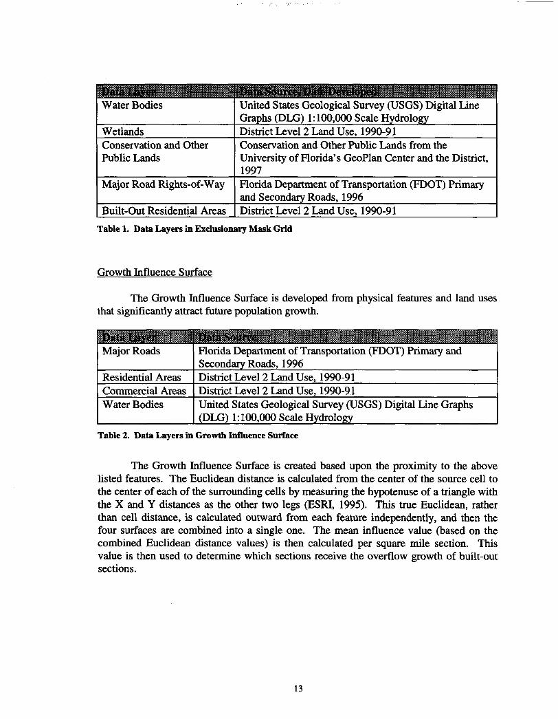
Water Bodies United States Geological Survey (USGS) Digital LineGraphs (DLG) 1:100.000 Scale Hydrology

Wetlands District Level 2 Land Use, 1990-91Conservation and OtherPublic Lands

Conservation and Other Public Lands from theUniversity of Florida's GeoPlan Center and the District,1997

Major Road Rights-of-Way Florida Department of Transportation (FOOT) Primaryand Secondary Roads, 1996

Built-Out Residential Areas District Level 2 Land Use, 1990-91

Table 1. Data Layers in Exclusionary Mask Grid

Growth Influence Surface

The Growth Influence Surface is developed from physical features and land usesthat significantly attract future population growth.

Major Roads Florida Department of Transportation (FDOT) Primary andSecondary Roads, 1996

Residential Areas District Level 2 Land Use, 1990-91Commercial Areas District Level 2 Land Use, 1990-91Water Bodies United States Geological Survey (USGS) Digital Line Graphs

(DLG) 1:100,000 Scale Hydrology

Table 2. Data Layers in Growth Influence Surface

The Growth Influence Surface is created based upon the proximity to the abovelisted features. The Euclidean distance is calculated from the center of the source cell tothe center of each of the surrounding cells by measuring the hypotenuse of a triangle withthe X and Y distances as the other two legs (ESRI, 1995). This true Euclidean, ratherthan cell distance, is calculated outward from each feature independently, and then thefour surfaces are combined into a single one. The mean influence value (based on thecombined Euclidean distance values) is then calculated per square mile section. Thisvalue is then used to determine which sections receive the overflow growth of built-outsections.

13

Growth Suitability Grid

The Growth Influence Surface is then combined with the Historical GrowthTrends Grid to create the Growth Suitability Grid. Existing residential land uses andother land uses that may be anticipated for conversion to residential are used to create anew grid in which future growth can be distributed. Those land uses include agricultural,forested, range, and open lands. The per section Historical Growth Trends and the meanvalues from the Growth Suitability Surface are then attached to the new Grid.

This new grid has considerably more land area in which to distribute futuregrowth. This is due to the fact that when growth is distributed in currently non-residentialland uses, there is no way to determine the spatial extent of that growth within thesection, so all of the land available for development is shown. Section build-out can stillbe calculated, but densities within each section are not known.

Distribution of Growth bv Section

The growth is calculated for each section over the specified period using the persection growth rates from the Historic Growth Trends Grid. This adjusted averagegrowth is added to the base year population for each section to derive the futuredistribution of that growth within the county. At this point, where the growth is occurringis actually more important than the total growth numbers.

As was anticipated, the majority of the projected growth moved further away fromthe current urban areas with each succeeding period. Over the earlier periods (1991through 1995, 1996 through 2000, and 2001 through 2005), most of the projected growthwas still clustered around current urban areas. Over the later periods however (2006through 2010, 2011 through 2015, and 2016 through 2020), much of the growth wasprojected to occur well outside the current urban areas.

Of course these estimates are based on current densities and development patterns,but as yet there is little indication that these are likely to change in the near future.Consumer preferences and developer costs drive these development patterns anddensities. Until the supply of land becomes scarce enough, thus increasing the cost ofland, or governmental regulations encourage denser development, we must assume thatthere will be no fundamental change in current development patterns and densities at leastfor the near future.

Normalize Growth with BEBR's County Total. Now that the relative distributionof the growth has been determined, this projected growth is then normalized usingBEBR's county population estimates. All the sections in the county are totaled. Themodel's projected growth for each section is divided by this raw total and multiplied byBEBR's county estimate.

14

Test for Build-Out. Each section is then tested to determine if it has exceeded itsmaximum capacity, or is built-out. If the base year population plus the projected growthdoes exceed the section's growth capacity, the growth will be calculated to equal thecapacity minus the base year population. A field in the table is then calculated equal tothe excess projected growth. This field containing the excess projected growth issummed for all the sections in the county.

Redistribute Any Growth Exceeding Capacity. Sections that have not exceededtheir capacity for growth are then selected one at a time in the order of their mean growthinfluence value. Each is again normalized to absorb any excess projected growth. If asection becomes built-out at this stage, the additional projected growth is distributed tothe section with the highest suitability value that can absorb that growth.

Single and Multi Family Unit Calculations. When the growth is fully distributed,the end year total population is calculated. Single family and multi family units are thenestimated from the population change to compare with projections from utilities thatmeasure growth in units as well as in population.

Updates in Model Inputs from Prior Model Periods

Each period over which the model is run for Orange County results in populationgrowth. This additional population may cause one or more sections to become built-out.If this occurs, those areas are added to the Non-Developable Lands Exclusionary MaskGrid and to the Growth Influence Surface.

Integration of Built-Out Sections with the Mask Grid

The sections that have become built-out from the previous modeling period arethen put into a new mask grid to exclude them from receiving growth in future periods.

Integration of Built-Out Sections with the Growth Influence Surface

This new Exclusionary Mask Grid is also added to the Residential Land Use Grid,so that the Residential Proximity Surface may be recalculated for future periods. Thiswill increase the growth potential of sections that are near built-out areas in future modelruns.

Final Output of Model

The final grids containing the distribution of population growth by section arethen summarized by Utility Service Area Boundaries. These boundaries are the ServiceArea Boundaries of water-providing utility companies. Because these boundariesgenerally overlap section lines, further processing of the data is required.

15

The assumption of population being evenly distributed within a given section splitby a Utility Service Area Boundary did not appear to be a significant problem. In mostcases, the Utility Service Area boundaries spanned many sections, so any errors due tothis forced assumption were diluted by the growth from sections completely containedwithin the boundaries.

Utility Service Area Growth Summary Grids

For each period, the population and dwelling unit growth and end year totals bysection are divided by the number of 30-meter grid cells within the section to derive per-cell growth and per-cell end year population and unit totals. The Utility Service AreaBoundaries are then overlaid, and the per-cell values are re-aggregated to theseboundaries. Separate grids are created for each population, single family, and multifamily growth period and each end year total, which are then joined together and exportedto a dBASE file for later import into Microsoft Excel.

This methodology assumes an even distribution within the section. Althoughpopulation distributions within a given section could vary a great deal, it is not possibleusing this data to account for varied densities within a given section.

Output Tables

The spatial results (the final Utility Service Area Growth and Population Grids)can be displayed to indicate projected patterns of future growth, but the output tables (thegrid Value Attribute Tables) are important without their Spatial Element. The tables areused to "plug in" to the St. Johns River Water Management District's Future WaterDemand Model, and they are useful for comparison with projections made by the water-providing utility companies. For this reason, the tabular results are further manipulated tofacilitate these efforts.

The Value Attribute Tables of all 12 final Utility Service Area growth andpopulation grids are joined together. A Frequency is run on the combined ValueAttribute Table, resulting in a table with a unique record for each utility company. Theresulting Frequency table is then exported in ARC/INFO® to a dBASE file. The dBASEfile is imported into Microsoft Excel, formatted, and e-mailed to the St. Johns RiverWater Management District. There it is used to "plug in" to their Future Water DemandModel and for comparison with projections received from the water-providing utilitycompanies.

The acreage for each of the service areas was included to compare with thegrowth. Some of the projections are very small, but eight of the service areas in OrangeCounty alone are less than ten acres. The District required growth numbers, but thegrowth results may be more meaningfully compared if normalized by acreage (growthdensity).

16

Verification of Results

The model results are then compared with other projections made by BEBR, localplanning agencies, and the utilities themselves.

BEBR. Before the model's projections are normalized, this county total iscompared with BEBR's county total. The average of the four methods was five percenthigher on average than BEBR's estimate. Although the model was designed to allocaterather than project population, achieving only a slight difference in projections inspiresconfidence and is worth noting.

Utility Companies and Local Planning Agencies. The growth estimates of theTAZ-based models employed by many of the various utility companies and local planningagencies are compared with model results. These are perhaps the most importantcomparisons, because future permitting is done at this level

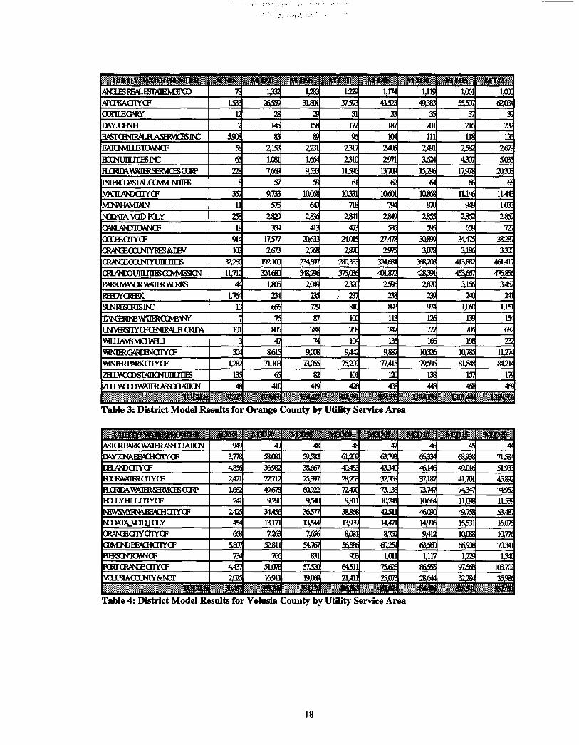
To compare the model results with those of TAZ-based models, the TAZ resultswere summarized by Utility Service Area boundaries, and these were compared with themodel results (which were already summarized by Utility Service Area boundaries).Tables 3 and 4 contain the model results for Orange and Volusia Counties (respectively),Tables 5 and 6 contain the TAZ numbers for Orange and Volusia Counties, and Tables 7and 8 contain the percentage differences between the two models.

17

7* 1332 1283 122 1,174 1,119 loottfOKAOIYCF 1433 2^55 31̂ 01 43523 493S3 55407 62,0*oornEGwy 12 2 31 33 37 3£DWKWJH 145 15E 172 187 201 216 23CEASTCBflRALHAraVKBSBt S a 104 11

2,153 2231 2317 2,406 2491 2582 267EBDCNTJIILIIIBSINC e 1,081 23K 2971 4307 5,03fHOTEAWSOHWERVKESCCFP 22 915* 13,703 15,79C 17̂ 75 2030EMEROCHSD4XIMV1NIIES 57 5 61 62 6!

357 9,733 10,03 1Q331 10,601 1Q8S 11,14! 11.4CMNVHAMMN TK 794 87C 1,01

2S 2841 2849 Z8S 2862 2,883S 412 472 535 5K 6S 727

17377 20,6* 24015 27,478 301895 34,475 381287CRANZCOJNIYFBS&EEV 10E 2673 27S 287C 2975 3,075 330(OWiSCECOMIYUIlLniBS 192,1(1 2H897 28038 413̂ 882

11,71: 3246X 34Si79( 375,<H 401̂ 72 428391 453̂ 667 476.85E2,0* 232 2596 287C 3,155 3,46

RHDif CREEK 1,7& 2* 235 237 238 23S 240 241SLNFffiOOSffC es 7Z 81( 893 1,060 1,151

87 MI 113 126 139 15U^VERSTIYCFCENIRALEl£Hn\ 101 80f 7S 7S 747 727 705\MLUANBMCHAELJ 47 104 135 166 198 23C\MNIERQWCENCnYCF 9,442 9,883 1Q326 1Q785\MMERPy\RKOIYCF 71.ME 73.0S 77,415 79 81,843 8421'ZEUANODSCOICNUIILniES 13f 82 101 12C 138 157 17

42 43 448 458 46!

Table 3: District Model Results for Orange County by Utility Service Area

MX>20ASICRPARKWOERASSOOAIKN 949 48 47 45 44

3.77S 59,582 6UCE 63,792 663* 68,92 714*EHJUNXHYCF 4856 36582 38̂ 67 40,483 4334C 46,146 49,016 51,932

2421 22,71: 25397 28^63 32,766 37,187 41,701 45,8921,62 6Q922 72,470 73,15 73,747 74347 74952

HILYHLLCnYCF 241 9,29( 9,5* 9311 1Q241 10,664 11,03 114K2425 34.4S 36577 38,8« 42411 46.C9C 49,755 53,487

454 13,171 13̂ 544 O939 14,471 14996 15431 16075CRANCEOIYCnYCF 658 7^55 8,752 9,412 1QOS 1Q77(CFMlOEEACHCnYCF 51807 52,811 54,767 56,88f 6Q251 669S 7Q341HERSCNTOWCF 7« 831 90B 1,011 1,117 us 134CPCRTCRANGEOIYCF 4437 51,075 5742C 64511 75^2 86555 97.5S 103,70:vouaAoiMY&Nar 202* 16911 190® 21,411 25,072 28,64! 222*

4S4.4STable 4: District Model Results for Volusia County by Utility Service Area

18

ArOBSFEHLESIXEMarCDffCPKAOTfCFCDTHECWWEATCSNHEASTCB<nRALHAS5!VKESIN:BOCNVmETCWNCFBOCNUDLniBSIICHTROVWOHiSBMCECaPIMHraVSEmMKJSTIIBSMVILWXnYCFMNVHAMIAIN^aMD^.\aDKLYCBKLiVNyiCMNCFOOCEEOIYCFCRANZO1MYFBS&EEV(XANZaXNIYUnLTIIBSCHLAvTOUIILrDESCEMVtSSlCNPARKMVMRWOHIWMSRKBfCRffiKSUMttfiCKlSINCTSNSaNEWOH«IMWWINNHSOTCFOaflRALHOTIAWUIAN*iMCH«JWNIHMMimCnYCFVMNIHlPARKCnYCFZHLWJDSIXnCNUIILraBS2BLLWXDWOHiASSOCL«aKN

' , jt**^*^ /3tim8

781533

122

5.9M58«

228

26711

258K

9UICE

3226C11,712

41,7*

121

101-.

»UK

13!4!

!fts>igai

123323,051

262139

1,1452,771

8373*

16212,461

4751488

13116,0363271

191,101328^62

1̂ 9E582218

3C1,167

539,6£

72JSK29

329ts<lpj@H

U18323*

401155

1,438293f

115&61C

19713,4*

57515C

171l&ffK3,436

238,41̂351466

W5S232

3£1,19!

871Q1472,78

3132

, Tfiyrc

uoe41,747

535151

1,7313,ia

149381

23214,422

675M»211

2aiu3#E

285,74137433

23<59524637

1222121

1Q6S72,885

351

321l^il«5SK

1,1875WK

67?14!

2,C&3^263

is;1Q14

267153»

7761,45125

22,1473,767

333.0C6397332

Z552602284(

V250155

11,15872,953

38327

:::̂ S6&*»

1,1726Q434

817142

23173,427

2161Q9K

30E16376

87tMOf

29C24,1853,931

3SQ30B42Q192

237260f27^4

127?18E

HfiSfi73,086

41326

vl..»BW

1,15769,7*

955135

2,6103492

25C11,685

3361735E

9771362

33C262*40*

4Z7,6Z443̂ 137

3,1936142847

130E222

12,17773,1*

42325

^KMjtt

l,16f8Q19:

1.10E137

2,9413,9S

2%12/H

31192811,08!ya

37!28,95:42«

481,93'482,11:

34*73730!51

13K261

133376,85

a33"

•s;!£BB$(Table 5: TAZ-Based Model Results for Orange County by Utility Service Area

ASICRPAHCWOHiASSOaAIKN 9« 182 171 159 147 136 112DWICN^EBOKHYCF 3,77! 71297 81,101 90347 1CQ651 11Q40C 119,701 128,95;EaANDOIYCF 38,977 4260 46,193 49337 53,423

2,421 18283 2124 24,186 27,147 30,095 32S«5 35,8a37405 3943S 41459 4349S 451611 4745C 49,47f

HlLYHLLaiYCF 241 112* 1139 12412 13.13C 13,741 14338 14,92;2,425 2139C 24252 27,097 29^66 32315 3837:

454 15̂ 85 17474 194X 21345 23232 25,071 26,saCRAMEOIYOIYCF 68t 9^03 113CE 12,767 13,716 14,6* 154*CHVOOEE^HOIYCF 5307 424QC 47.7M 52,885 58,(H 63275 68342 733»HB8CNTCWNCF 734 618 632 645 65S 673 685 69!PCRTCRAfCEaiYCF 4,437 45,485 51,472 57,434 63,41$ 6938C 74,01 78,61!

2,02 17581 19274 204* 21,8« 23.1K 24365 254*

Table 6: TAZ-Based Model Results for Volusia County by Utility Service Area

19

78 ao?? 539? 229? 1.195 4395 8395 1429!AKJKAOIYCF 1333 15295 1.895 1Q095 14595 18395 20395 2269!

12 893% 94295 95.19? 95.795 96.195 9539!1.99? 1359? 28.195 41395 56395 69395

5506 92.89? 93.89? 9439J 94.99? 9529? 9539? 95.795BaCNVOlEICMNO? 5S 2239? 24.09? 2539J 2639? 2739? 28.19? 3279!BOCNUmillESINC ffi 1234.69? 1347.09? 146089? 1532495 1577.895 1622895 166059!

22 229? 1079? 23.69? 35.195 44.79? 6009!

7019? 73.79? 76.895 8049! 8159!MVnDVNDOIYCF 357 21.99? 25.195 28.495 31295 33.695 3559? 40695

MN4HAMJAIN 11 21.19? 11.89? 649? 239? 079? 299? 4.8952$ 78.19? 89.79? 9639? 103.195 110195 90995

OVKLANDTCWNCF 174.09? 14139? 124295 114.095 10529? 99.79? 9239!914 9.6% 1429? 19.495 24.195 27595 31395 32295

OVN3EODLNIYRBS&EEV 10E 1839? 19.49? 2039! 21.095 21.795 22295 23295CRANCEODLNIYUHLniBS 3226C 059? 139? 1.995 2595 3295 329? 4395O^ANDOUIIUIIBSOCNMSSICN 11,71: Q19? 1.195 2095 2495 1.195PARKMVNCRWAimWKKS 1339? 7.19? 31895 1.795 0195 1295 2395KtmfCRHK 1,7ft 6009? 60295 6059? 60795 60995 67395SLNREXKISINC 200.99? 21429? 22939? 24339? 25539? 268.195 277.495

15339? 163.69? 17039? 18259? 186.49? 195.795 202095101 30.99? 34.19? 37295 40295 43.195 46.095 5L095

\MUJA\fiMCHAHJ 1139? 14.99? 14.09? 12995 1229? 1129? 11.195\MNIHlGMCBSICnYCF 304 106% 1129? 11.495 11.495 11395 11.49? 15.69!VMNimPARKOIYCF 049? 3295 6195 9.095 11.99! 9.695ZELLwrDSixncNuinrnB 135 124.19J 215.895 236.69! 265.19? 25809!

33.995 37.495 40995 4049!

Table 7: Differences Between District Model Results and TAZ-Based Model Results for OrangeCounty by Utility Service Area

73.195 7L99! 6528 63.795 6L19!3177? 4249!

I&ANXHYCF 48* 5195 9395 12495 13.08 13.05 13.995242 16995 2Q79! 23.69!\f& 3259! 54195 744^ 67.895 6L795 5L59i

ffLLYHILCnYCF 2L69i 22093 2249! 2269! 2279?24Z 6L195 4L995 4059! 39.491

22995 28.495 32295 35595 3&095 4Q29iOMNKJIYOIYCF 26795 3L695 3L495 3L495 3L19! 3Q89!

5337 2439! 7.69! 3795 049! 2195 419!HH8CNIDW4CF 734 23.99? 3L595 4Q095 53.495 66095 79.49! 92395PCRTaWNKHYCF 4437 12395 1L89! 12395 19395 24895 3L89! 38.39i

202" L19i 429! 23.995 32595 4Q6J

Table 8: Differences Between District Model Results and TAZ-Based Model Results for VolusiaCounty by Utility Service Area

To translate the section-level results to Utility Service Area boundaries requiresthe assumption of an even distribution of population within the developable areas of eachsection. A section could have the majority of its population on the part of the sectionwithin one service area, but the model would only allocate the section's average

20

population per grid cell times the section's total developable grid cells in that UtilityService Area. For example, if 20 percent of a section's developable area and 90 percentof a section's population fell into a particular service area, only 20 percent of thepopulation would be allocated. This limitation is more likely to affect the results forutilities with smaller service areas, as they have less margin for error.

The differences by Utility Service Area in Orange and Volusia Counties werequantified and studied. Clearly a certain percentage of these differences is due toboundary errors. This problem is greatest with smaller Utility Service Areas, suggestingthat the variation in the densities within sections straddling Utility Service Areaboundaries is a major factor in the discrepancies between the model and the utilityprojections.

When only considering utilities with 1,000 or more acres, this boundary errordecreases significantly. The average error in 1990 drops from 92.4% to 28.6% in OrangeCounty, and from 26.3% to 23.0% in Volusia County.

tftFKAOIYCF 143: 1523 1009! 1839! 2159!EASTCB^R^HAfflWKESINC 593 94595 9499! 9529! 9559! 95.7%CRAN3EOOLMYUIIIIIIB 059! L59! 1.995 259! 3225 328 439i

11,712 1.295 019! L19! 209! 2495EHDTCFEHC 6Q79! 6739!\MNimPAPKCnYCF 1282 229! 0495 3i2Si 619! 9.09! 11.99!

Table 9: Differences Between District Model Results and TAZ-Based Model Results for OrangeCounty for Utility Service Areas of 1,000 Or More Acres

3,778 1859! 26595 32.635 39.99! 4249! 4459!EaAMXHYCF 4856 5195 9395 1249! 13.09! 13.05 13.99! 140?!HXEWOHUJIYCF 2421 16995 20795 23.69! 2649!

WS2 3259! 54195 7449! 67.89! 6L795 5649! 5L59i2425 6L19! 43.49! 4L99! 40595 39.89!

CRNOCEBOKJIYCF 5807 2439! 14895 7.69! 379! 0495 219!PCRTOWCECnYCF 4,437 1239! 1239! 19.39! 2489$ 3L89i\aiHAGOLNIY&N3r 2025 L195 429! 1489! 23.9?! 3259!

Table 10: Differences Between District Model Results and TAZ-Based Model Results for VolusiaCounty for Utility Service Areas of 1,000 Or More Acres

When only considering utilities with 10,000 or more acres in Orange County and4,000 or more acres in Volusia County, this boundary error further decreases. Theaverage error in 1990 drops from 92.4% to 0.9% in Orange County, and from 26.3% to13.9% in Volusia County.

21

Table 11: Differences Between District Model Results and TAZ-Based Model Results for OrangeCounty for Utility Service Areas of 10,000 Or More Acres

4856 5.19! 939! 1249! 13.09! 13.69! 1199! 1409!CHVQOEE^HCHYCF 5^807 1489! 7.0! 179! 219! 419!PCKrCRANCEOIYCF 4437 1239! 1L89! 1239! 1939! 3.89! 3L89! 3839!

1 - .Table 12: Differences Between District Model Results and TAZ-Based Model Results for Volusia

County for Utility Service Areas of 4,000 Or More Acres

22

CONCLUSION AND DISCUSSION

This model was a success in that it developed a methodology to distribute countylevel projections to an area small enough to be useful to the St. Johns River WaterManagement District. The raw projections, before normalization, were encouraging inthat the results at the county level were very close to those developed by BEBR. Furthertesting will be required to adequately validate this model, but the results comparefavorably to those of most of the larger utilities. As expected, growth in Orange Countyis projected to be strongest around the urban fringe around Orlando, particularly west andnorthwest of Orlando. The same phenomenon was seen in Volusia County, where thehighest growth rates were north, south, and west of Daytona's core urban area.

Integration of Built-Out Sections with the Mask Grid. Although the rates at whichsections become built-out produces reasonable results, no attempts to validate theseresults have been made as yet. The method used to calculate build-out will changesomewhat when digital future land use maps are integrated into this step later in theProject. Validation will occur after this change is made.

Integration of Built-Out Sections with the Influence Surface. It is also reasonableto assume that as residential development occurs, it generally attracts furtherdevelopment: commercial, industrial, and more residential. Existing employmentopportunities, services, and infrastructure all contribute to the increased "attractiveness"of land near existing developed areas. Although land farther away from currentdeveloped areas is generally cheaper, and although it is attractive to some for its pristinequalities, the possibility of development is less than that of similar areas in closerproximity to current development. For this reason, the added weight given to built-outareas by adding them to the Growth Influence Surface at the end of each period in themodel is justified.

Final Output of Model

The utility companies have used different methods for projecting future demand intheir service areas. Some utilities made their own projections, but many used projectionsfrom local planning agencies or hired consultants to make the projections for them. Someof the projections may be good and some may not. The comparison of this model'sresults against those of the utility companies is useful, but even if the estimates are veryclose does not mean they are accurate. Future investigation into the methods of eachutility would be useful in gauging the reliability of their results.

Although the utilities have more knowledge of their service area, it is believedthat this model is a more comprehensive measure of the factors influencing populationgrowth. If local information such as Developments of Regional Impact (DRIs), buildingpermit activity, local tastes and preferences, etc., is integrated with the model at a later

23

date, any discrepancies between the model and the utilities should not lessen confidencein the model.

However, the TAZ-based models are likely a more accurate reflection of the baseyear population. The model's projections are generally close to those made by the TAZ-based models. When only considering the larger utilities (thus reducing boundary errors),the average error in 1990 is 0.9% in Orange County and 13.9% in Volusia County.However, the discrepancies among the smaller utilities are much larger. This givesevidence to the conclusion that the variation in the densities within sections straddlingUtility Service Area boundaries is a major factor in the discrepancies between the modeland the utility projections.

Future Improvements to the Model

Any future improvements to the model should include updates in the data setsused in the model, further refinements in the methodology, and the enhancement of theuser interface.

Data Updates

Some of the data sets used in this model are out of date. They were used becausethey are the best data currently available, but many can be updated in the near future.

Department of Revenue's Property Appraiser Data. The GeoPlan Center at theUniversity of Florida will be receiving the 1996 update of the Property Appraiser data setfrom the Florida DOR in the next few months. When this becomes available, the baseyear can be changed to 1995.

Level 2 Land Use. The District is in the process of updating its land use data, andthe new version should be ready by late 1998 or early 1999. This is especially importantif the base year is changed to 1995, so that the residential land use will be current.

Future Land Use. This has recently become available from the District PlanningDepartment. It was created from local government future land use maps (FLUMs), andcan be used to enhance the methodology for calculating build-out.

USGS 1:24.000 Hydrology. The 1:24,000 hydrology layer has recently been madeavailable from the United States Geological Survey (USGS). It is more accurate than the1:100,000 hydrology currently being used by the model, so it can replace the oldhydrology in the very near future.

Conservation Lands. The conservation lands are updated frequently by theDistrict and the GeoPlan Center. Any additions to this layer are extremely important andcan be integrated into the model as they become available.

24

Refinement of Methodology

Currently the model makes good section level projections, but is not yet a trueforecasting model. Although some local knowledge is integrated into the methodology, itdoes not presently incorporate enough local knowledge of DRIs, building permit activity,local tastes and preferences, and the like. Andrew M. Isserman writes that "forecastingshould be an interactive process, involving local information, staff participation, andcitizen involvement. Data and methods can focus and discipline the effort, but in the endforecasting is also part history, part storytelling." (Isserman, 1993). Robert Hopkins addsthat a true forecast "predicts the most likely future, a future which may well be acontinuation of existing trends or may predict a marked change in direction." (Hopkins,1992). Any such marked change could put the planners at the District at a disadvantage.Any continued work done on the model should focus on this important effort ofincorporating local knowledge and comments, bridging the gap between a projectionmodel and a true forecasting model.

Determination of Build-Out. Neither the future land use maps nor the currentmethodology alone inspires a great deal of confidence in determining build-out. The bestmethod given the available data and budget and time constraints would be a combinationof the two methods. The current statistical method based on existing densities would actas a check and balance for the future land use, which in many cases is unrealistic. Thefuture land use could be useful, although the accuracy is somewhat variable. In someareas, the future land use present a more aggressive rate of population growth thanobserved in the BEBR county population projections.

Adjust Base Year Grid. Because the TAZ-based models are likely more accuratereflections of base year population, the model's base year grid with population estimatedfrom parcels will be adjusted with either TAZ data or the original census block data.

Improvement of User Interface

Future improvements to the model could make it both easier to use and morefunctional. Porting the model to a Windows-based software package would enable non-technical users to run the model. Adding more menus for user input would allow userswith knowledge of the area being modeled to influence model results.

Conversion to ArcView® 3.0 GIS. All of the functionality provided byARC/INFO® to run the model can be replicated using ArcView® 3.0 GIS. ArcView is auser-friendly desktop software package that is a fraction of the cost of ARC/INFO®. Ithas an easy-to-learn windows interface, so that managers and planners who are not GISexperts may run the model themselves on their own PCs. The model could be automatedthrough Avenue™, Arc View's object oriented programming language. It could also bedemonstrated at public meetings much more easily than the UNIX ARC/INFO®-basedmodel, the District intends to eventually port this model to ArcView.

25

Additional Menus for User Input. Future plans for the model also includeproviding for additional input from users. Menus to allow users to increase or decreasethe influence of a particular feature and/or method or to add an entirely new feature willprovide further sensitivity analysis for these features and/or methods. For example, if alocal government official was aware of a new DRI or a considerable increase in buildingpermit activity in a particular area, the user could digitize the feature or area, weight itaccordingly, and input it directly to the model.

The Future of Growth Modeling and GIS

The tools for creating, processing, analyzing and outputting digital data areadvancing geometrically. Increased processing power and data availability coupled withimprovements in software applications make possible projects that were only recentlyunthinkable. As the tools improve, so will the information and models that they aredesigned to build.

This will be true of future efforts to model population growth as well. Bettermodels will be developed to forecast growth over very small areas that will use existing,current, high quality data sets. Many will allow a high level of user interaction forsensitivity analysis and calibration. They will also be easy to use, because the end usersin most cases are manager or planners not well skilled in GIS.

Better information leads to better decisions. Too often decisions are madeon insufficient or in accurate information. The future promises more and betterinformation, and more and better tools to create, process, and analyze that information.Huxhold affirms that "the value of information increases the more it is shared anddisseminated" and points out that "information that is not used is useless" (Huxhold,1991: p.4). As valuable as good estimates of future growth are, there will be a premiumon accurate models for forecasting population growth in the years ahead.

26

REFERENCE LIST

Alexander, John F., Jr., Paul D. Zwick, James J. Miller, and Mark H. Hoover (1984),Alafia River Basin Land and Water Use Projection Model. Vol. I, Department ofUrban and Regional Planning, University of Florida, Gainesville, Florida.

Environmental Systems Research Institute, Inc. (1995), ARC/INFO On-Line Help Files.ARC/INFO Version 7.0.3, ESRI, Redlands, California.

Environmental Systems Research Institute, Inc. (1990), Understanding GIS: TheARC/INFO Method. Redlands, California.

Forrester, Jay W. (1961), Industrial Dynamics. MIT Press, Massachusetts Institute ofTechnology, Cambridge, Massachusetts.

Hopkins, Robert (1992), "Using GIS in Modeling Urban Growth", A DissertationAbstract in the Department of Urban and Regional Planning, University ofFlorida, Gainesville, Florida.

Huxhold, W.E. (1991), An Introduction to Urban Geographic Information Systems.University of Wisconsin, Milwaukee, Wisconsin.

Isserman, Andrew M. (1993), "The Right People, the Right Rates: Making PopulationEstimates and Forecasts with an Interregional Cohort-Component Model", Journalof the American Planning Association. Vol. 59, No. 1, Winter 1993, AmericanPlanning Association, Chicago, Illinois.

Pfeiffer, P. E. (1961), Linear Systems Analysis. McGraw-Hill Book Company, Inc., NewYork, New York.

Scholten, Henk J., and John C. H. Stillwell (1990), Geographical Information Systems forUrban and Regional Planning. The GeoJournal Library, Vol. 17, KluwerAcademic Publishers, Dordrecht/Boston/London.

Scoggins and Pierce, ed. (1995), The Economy of Florida. The Bureau of Economic andBusiness Research, University of Florida, Gainesville, Florida.

Silverman, David (1993), Interpreting Qualitative Data: Methods for Analysing Talk.Text, and Interaction. SAGE Publications, London, England.

Sipe, Neil G., and Robert W. Hopkins (1984), "Microcomputers and Economic Analysis:Spreadsheet Templates for Local Government", BEBR Monographs. Bureau ofEconomic and Business Research, University of Florida, Gainesville, Florida.

27

Smith, Stanley K., and June Nogle (1998), "Projections of Florida Population by County,1997-2020", Florida Population Studies. Vol.31, No. 2, Bulletin 120, January1998, Bureau of Economic and Business Research, University of Florida,Gainesville, Florida.

Star, Jeffrey, and John Estes (1990), Geographic Information System: An Introduction.Prentice-Hall, Englewood Cliffs, New Jersey.

Wiggins, Lyna L. and Stephen P. French (1991), GIS: Assessing Your Needs andChoosing a System. Planning Advisory Service Report Number 433, AmericanPlanning Association, Washington, DC.

28

APPENDIX AARC MACRO LANGUAGE (AML) PROGRAMS

The model was built using ARC/INFO® GIS software developed byEnvironmental Systems Research Institute (ESRI). The Arc Macro Language (AML)programs written for the model described are as follows:

1. SETUP.AML. Copies input coverages, grids, and INFO tables from varioussources to be used in the model. Converts coverages to grids, and attachesvector attributes.

2. START.AML. Prompts the user to select the county or counties to bemodeled, sets path variables, and calls other AMLs to be run.

3. SETWIN.AML. Sets initial Grid settings. Called by other AMLs when Gridcommand is issued.

4. MOD.AML. Main model AML. Creates grid and dBASE file of populationand growth by square mile section.

5. SUM WSA.AML. Summarizes section numbers created by MOD.AML bywater utility service area boundaries.

6. SUM TAZ BY WSA.AML. Summarizes TAZ-based model results by waterutility service area boundaries (to compare against the District model results).

7. SUM TAZ.AML. Summarizes section numbers created by MOD.AML byTAZ boundaries. Originally written to compare the District model's sectionnumbers against TAZ-based model results. Later concluded that summarizingthe TAZ-based model results by utility service area made more sense, so thisis no longer used.

Additional AMLs and menus used during the modeling process are organized intothe following workspaces:

1. W OLD AMLS. Contains older versions of model AMLs for futurereference.

2. W OLD MENUS. Contains menus no longer used (to graphically selectthe county to be run, to click on the period to be run, etc.). It was determinedthat the model will be run in advance of viewing/analyzing the results, andthat the model will normally be run by a District employee familiar withARC/INFO®. Therefore, a batch process is preferable to an interactive,menu-driven one.

3. W UTILITIES. Contains utility AMLs for use with model data sets (toproject or reproject, copy, kill, etc.). Projection files area included in theW_PRJ_FILES directory under WJJTILITIES.

Anyone familiar with ARC/INFO® and AML programming will be able to usethe above AMLs. In some cases, minor edits may be required to accommodate for futurechanges in input data attributes, locations, etc. This should not present a problem, as theprograms are well-commented and easy to follow. The following pages are printouts ofthe AML programs.

29

APPENDIX BDISK STORAGE AND DATA REQUIREMENTS

The data sets (including the tax data) varies per county from 30 MBs (Baker) to300 MBs (Orange), totaling approximately 1.8 GBs for the 18 county area. Additionalmemory is required for processing, so a minimum of 2.0 GB should be reserved for themodel.

The required input data sets to run the model are contained in Table 13.

Tax Data INFO Table TAX DATA Florida Department of RevenueCounty Boundaries Coverage BOUNDARY United States Census Bureau TIGER

Line FilesSection Boundaries Coverage(from the Public Land SurveySystem Township, Range, andSection lines)

PLSS Florida Resources and EnvironmentalAnalysis Center

Major Roads Coverage(Primary and Secondary)

DOTRDS Florida Department of Transportation

Level 2 Land Use Coverage LULEVEL2 St. Johns River Water ManagementDistrict

Water Bodies Coverage HYDRO United States Geological SurveyDigital Line Graphs (DLG) 1:100,000Scale Hydrology

Conservation and RecreationLands Coverage

CLAND GeoPlan Center and various WaterManagement Districts

Water Utility Service AreaBoundaries Coverage

WSA St. Johns River Water ManagementDistrict

Transportation Analysis ZoneBoundaries Coverage

TAZ St. Johns River Water ManagementDistrict from the East Central FloridaRegional Planning Council

Table 13. Input Data Layers Required to Run Model

30

The location of the input data layers are shown in Table 14.

%rootpath%<countyname>/data/covers

%rootpath% District/data/covers%rootpath%<countyname>/model/taz

PLSS, DOTRDS, LULEVEL2,HYDRO, CLANDWSATAZ

Table 14. Location of Input Data Layers Required to Run Model

31