Abstract Brain injury resulting from exposure to blast continues to be a significant problem in the military community, often leading to death or long term disability. The presence of high frequency energy content in pressure waves generated in explosive blasts necessitates understanding the transmissibility and damping characteristics of skull bone. Current finite element models (FEM) of the skull do not include material damping and therefore fail to capture the correct attenuation spectrum or rate dependency of skull bone.

Cylindrical through-the-thickness specimens of skull bone were obtained from ten adult (55 ± 10 years old) male post-mortem human surrogates. A test apparatus was developed to apply cyclic loading to potted cores at frequencies ranging from 1 to 50 kHz using a piezoelectric shaker. High bandwidth transducers were used to record accelerations and forces at the boundary. A lumped mass model was optimized to match the recorded boundary conditions.

This paper reports composite material properties of the skull as a frequency dependent complex modulus. The calculated material loss tangent was distributed in a log-normal fashion and ranged from 0.027 to 0.194 (95 % CI). A generalized Maxwell model, represented using a Prony series has been developed and the model parameters have been reported. Keywords generalized Maxwell model; adult human skull, rheometry, transmissibility, viscoelastic

I. INTRODUCTION

The study of viscoelasticity of bone began in 1970s. Viscoelastic properties obtained from creep and relaxation studies for long durations [1-2] can be used to predict behavior at low frequencies and are not relevant for dynamic events. During the same time, an instrument developed for observation of torsional stress strain behavior of small specimen was used to study viscoelasticity of pure compact bone [2]. This device was refined to deliver bending stress [3]. Yet other studies looked at decay of free vibrations [4]. All these studies were limited to pure cortical bone. Moreover these studies suffered from small number of specimens tested and were capable of frequencies up to only ~ 1 kHz. Only a few researchers have attempted to characterize composite whole bone response ([5-6]). However they have used animal whole bones and are very limited in numbers.

The study of brain injury due to explosive blasts requires the understanding of the skull behavior under somewhat different circumstances. Blast pressure is known to have significant energy content at frequencies of up to 20 kHz. Therefore data at larger frequencies is required. Reference [4] provides data at this frequency range for pure cortical bone. Skull bone has a sandwich structure with two dense cortical layers interspersed by a porous cancellous layer. It may be expected to behave differently due to the presence of pores and fluids. Current Finite Element (FE) models of the human skull have a mesh resolution of ~ 5 mm, which is close to the thickness of the skull. Therefore they sometimes have only one element through the thickness. A characterization of the composite response of the three layers of the skull will therefore be very valuable. This research develops a methodology for characterization of damping properties and attempts to provide a linear viscoelastic model of skull bone which exhibits correct response under loading conditions typically seen in explosive blast events.

Sourabh Boruah is PhD student in Biomechanics at University of Virginia in Charlottesville (phone: 434-296-7288 ext.115, fax: 434-296-3453 & e-mail: sourabh@virginia.edu). Damien L. Subit is Senior Scientist in the Center for Applied Biomechanics. Jeff R. Crandall is Professor in the Department of Mechanical and Aerospace Engineering. Robert S. Salzar is Principal Scientist in the Center for Applied Biomechanics at University of Virginia in Charlottesville. Barry S. Shender and Glenn Paskoff are Engineers at the Human Systems Department, Naval Air Warfare Center Aircraft Division, Patuxent River, MD.

Development of a material model to simulate through-the-thickness transmission of vibration in the adult human skull

Sourabh Boruah, Damien L. Subit, Jeff R. Crandall, Robert S. Salzar, Barry S. Shender, Glenn Paskoff

II. METHODS

Materials

Skull bone specimens were obtained from the calverium of ten adult male PMHS. The subjects, representing the 50th percentile adult male, were at an average 55 years old, 178 cm high and weighed 92 kg (TABLE I). All subjects were frozen post mortem and thawed for use. They were screened for common blood-borne pathogens and for pre-existing pathology that may influence bone properties. The University of Virginia cadaver institutional review board has reviewed and approved these test procedures. Clinical Computed Tomography (CT) was done for all subjects at a resolution of 0.625 mm in order to identify potential locations of harvesting skull bone specimens.

TABLE I PMHS ANTHROPOMETRY

Subject no. Age Height [cm] Weight [kg]

1 58 188 104

2 41 180 71

3 51 173 91

4 61 175 204

5 66 178 70

6 59 173 68

7 45 191 73

8 49 175 101

9 70 173 77

10 49 175 57

Ten locations were identified on the right half of the calverium for harvesting through-the-thickness cylindrical skull bone specimens (skull cores). These locations were distributed across the frontal bone and the parietal bone. Following thawing of the head, and removal of the scalp, these ten locations were marked on the skull surface (Fig. 1). Specimens were also harvested from symmetric points on the left half for another experiment. The harvest locations varied from skull to skull due the presence of un-suitable anomalies and curvatures and also to avoid sutures. The locations were measured for each skull using a 2 dimensional curvilinear coordinate system with the origin at the posterior end of the zygomatic bone. Fig. 2 shows the arrangement of this coordinate system. The first dimension is rear-wards along the intersection of the skull outer surface and the Frankfort plane and the second dimension orthogonal to the first, pointed towards the vertex of the skull.

Fig. 1. Ten test specimen harvest locations marked on the right half of the skull; two locations (8 and 10) not

Fig. 2. The harvest locations marked on a clinical CT rendering; measurements made along the skull outer

visible. surface relative to the zygomatic bone.

The calverium was removed using a circular oscillating saw and split into the right and left halves. Skull core specimens were then harvested using a circular abrasive drill bit on a bench drill press (Fig. 3). The bone was maintained hydrated with saline solution throughout this process to prevent excessive heating. This process yielded skull cores with a diameter of approximately 18 mm (Fig. 4).

Fig. 3. Skull cores obtained from right calverium using circular abrasive drill.

Fig. 4. A sample skull core.

Specimen Potting

The skull cores were potted in a minimal amount of polyester resin (Bondo, 3M, Maplewood, Minnesota) in order to provide two flat parallel surfaces for mounting the specimen on the test rig. The mass of the cores was measured prior to potting using an electronic scale (resolution 0.01 g). The two part filler was mixed using syringes to produce consistent potting material. It was then applied to the inner and outer tables and put in a jig to ensure flat and parallel surfaces (Fig. 5). The total potted thickness was measured using a vernier caliper.

Test Setup

The transmissibility test setup (Fig. 7) consisted of a piezo-electric reaction mass type shaker (Wilcoxon F7-1) exciting the test specimen against an index table. Test instrumentation included a piezo-electric load cell (Omega DLC 101-50) and a piezo-electric accelerometer (Brüel & Kjær 8309) on both sides of the test specimen. All data was sampled at 2 MHz using a Hi-Techniques Synergy-CS data acquisition system (DAS). All the components of the test system (the shaker, instruments and test specimen) were mounted in the same horizontal axis with the core outer table facing the shaker. An index table was used to accommodate specimen of various thicknesses. The setup was installed on a vibration isolation table. A schematic of the test setup is shown in Fig. 8.

Fig. 5. Potting of skull core in polyester using the jig device.

Fig. 6. Potted cores.

Fig. 7. Transmissibility Test setup; Shaker and shaker-side instruments (left); Index table and table-side instruments (right); please note that an aluminum placeholder sample is installed in the image on right.

The transmissibility test control system was designed and run in Labview (Fig. 9). A Rigol DG 1022 arbitrary waveform generator was controlled through USB using the National Instruments Virtual Instrument Software Architecture (NI-VISA) to calibrate the shaker power amplifier. Excitation signal amplitudes depended on the frequency of excitation and were predetermined to control oscillation near resonance spots and ensure a nearly constant displacement magnitude. There was feedback from the waveform generator confirming generation and cessation of excitation voltage. The Synergy-CS data acquisition system, controlled by Labview over the Ethernet using transmission control protocol (TCP / IP) provided feedback indicating amplitude of oscillation, which was used to ascertain steady-state vibration. The system was programmed to deliver vibration at frequencies ranging from 1 kHz to 50 kHz (evenly spaced in the logarithmic domain) and record steady state vibrations at each frequency. Frequencies at which sensor signals were saturated due to large amplitude of vibration were skipped.

Fig. 8. Schematic of test setup; skull core specimen sandwiched between two pseudo rigid tranducers consisting of mounting hardware, accelerometer and load-cell sprung mass.

Fig. 9. Schematic of the test control system; The controller (LABVIEW software in PC) communicates via TCP / IP with data acquisition system and via NI-VISA with the waveform generator.

Theoretical Modeling – Frequency domain

This step develops an effective, one-dimensional through-the-thickness response characterization in the frequency domain. This model is non-parametric and is free of any assumptions. The core sample mass (~ 2 g) is relatively small compared to the transducers at the boundary (~ 50 g each). The presence of the relatively massive transducers precludes straightforward calculation of material response. A simple lumped mass model (free body diagram shown in Fig. 10) has been used to account for the effects of transducer inertia. The material parameter sought is calculated from the single frequency dependent complex modulus *k (Fig. 11). The

Test Setup

Labview on PC

Synergy-CS DAS

DG1022 Wave Generator

Control System

NI-VISA connection VDC connection

TCP / IP connection

Shaker

Instruments

Sample Sample

Instruments

Table

Skull core specimen

Direction of motion

Mounting hardware

Accelerometer

Load Cell

governing equations for this model are shown in (1). The governing equations are solved to obtain structural parameter *k in terms of the known quantities (equation (2)).

Transducers:

sa or 1x : Shaker side acceleration

ta or 2x− : Table side acceleration

sf : Shaker-side Force

tf : Table-side Force Lumped Masses:

1m , 2m : Transducer mass Material Parameter:

*k : Complex spring constant (frequency dependent)

Fig. 10. Free body diagram of simple spring mass system used to model skull transmissibility in the frequency domain.

Fig. 11. Glossary of frequency domain model variables and parameters.

( ) 021*

11 =−−+ sfxxkxm

( ) 012*

22 =+−+ tfxxkxm (1)

( ) ( ) 02 12*

1122 =++−+− st ffxxkxmxm

( )( )12

2211*

2 xxffxmxmk st

−−−−

=

(2)

All of the variables may be expressed as a complex number in terms of their magnitudes and phases.

2

*

1*

1*

ω

ωωω

tisti

sti

sseAxeAxeAa −=⇒=⇒=

2

*

2*

2*

ω

ωωω

titti

tti

tteAxeAxeAa =⇒−=⇒=

tiss eFf ω*=

titt eFf ω*=

where, *

sA – Shaker-side acceleration *

tA – Table-side acceleration *

sF – Shaker-side force *

tF – Table-side force

(3)

Substituting variables from equations (3) in equation (2) and cancelling tie ω ,

( )( )

2**

***2

*1*

2ω

st

stts

AAFFAmAmk

+−−+

= (4)

The structural parameter on the left hand side of equation (4) is calculated at each frequency from the complex variables on the right hand side. Masses of the transducers (inclusive of load cell sprung mass, accelerometer and hardware) 1m and 1m have been measured directly. These complex variables are obtained directly from time-history data recorded during tests through discrete Fourier transform (DFT; typical magnitude spectra shown in Fig. 17). The frequency dependent structural parameter *k is normalized by cross-section area and sample thickness to obtain the frequency dependent complex modulus *E using relationship (5).

AlkE

** = where, l – Thickness of skull core sample

A –cross-section area of sample (5)

Theoretical Modeling – Time domain

In order to apply the frequency domain knowledge to predict response of the skull to an arbitrary event, a time domain model is needed. One of the most common models used for biomaterials is a generalized Maxwell

model (Fig. 12). The generalized Maxwell model is represented parametrically by its relaxation function (Prony series [7]). The parameters are described in Fig. 13. The Prony series was chosen since it is pre-implemented in most commercial FE solver packages and is readily applicable.

Frequency domain material parameter: *E – Complex spring constant

Time domain material parameters:

∞E – Long term structural stiffness

jE – Spring constant of j th Maxwell element

jβ – Decay constant of j th Maxwell element

Fig. 12. Frequency dependent complex modulus converted to generalized Maxwell model.

Fig. 13. Glossary of time domain model parameters.

The complex modulus of the generalized Maxwell model is represented in terms of the Prony series parameters in equation (6).

∑ ++= ∞

j j

j

iEi

EE well ωβω

max* (6)

For simplicity of comparison, parameters jβ have been fixed and ∞E obtained from lower rate

compression tests [8]. The Maxwell unit stiffness parameters jE are optimized to match parametric Maxwell

complex modulus wellE max* , obtained using equation (6), to frequency dependent (but non-parametric) *E

(from equation (5)) calculated from experiment data in the previous section.

III. RESULTS

A few examples of the experimental modulus and loss tangent from the experimental data are shown in Fig. 14. Although the objective was to capture data at frequencies from 1 kHz to 50 kHz, the entire spectrum could not be captured due to excessive vibration at certain frequencies and inability to attain steady-state due to the same reason. Outliers are seen typically at the higher frequency end and also at the boundaries of frequency domains of excessive vibrations (seen in all graphs in Fig. 14). The average loss tangent across the range of excitation frequencies of the 86 core samples (Fig. 15) has a median value of 0.074 (~2 to 20 kHz excitation frequency). Tan δ does not correlate with specimen or harvest location. At each frequency, the tan δ for all cores are distributed in a log-normal fashion. Therefore to show frequency dependence, the average and confidence intervals are built in the logarithmic domain. The dependence of tan δ on frequency and its 95 % confidence interval is shown in Fig. 16.

Fig. 14. Typical graphs showing change in magnitude of complex modulus (top) and loss tangent (bottom; logarithmic scale) with respect to frequency; dashed line shows a five term Prony series fit to the experimental data.

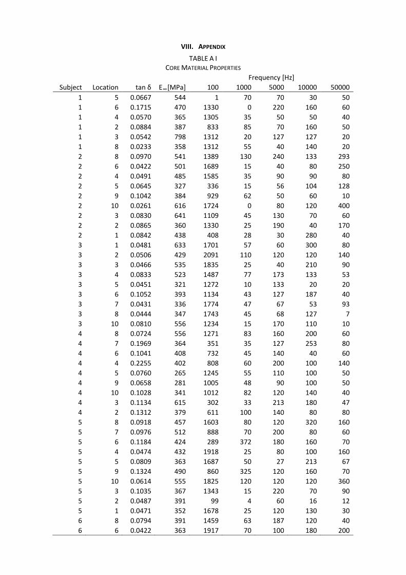
Fig. 14 also shows a five term Prony series fit to the experimental data (dashed line). The decay constants used and corresponding average stiffnesses for the 86 cores is presented in TABLE II. The Prony series function is found to be ill-suited to model experimental data that change fast with respect to frequency (arrow on top right; Fig. 14). Detailed core-wise material properties have been listed in TABLE A I. Since no tests were done below 1 kHz, all stiffness that relaxes slower than that are clubbed together in jβ = 100 Hz or 1000 Hz

depending on the magnitude of loss modulus at 1000 Hz.

Fig. 15. Material loss tangent (tan δ) for 86 through-the-thickness skull core samples, averaged across range of excitation frequency (~2 to 20 kHz)

Fig. 16. Loss tangent (tan δ); expected value (circles) and 95 % confidence intervals (gray bars) at different frequencies on vibration; note: tan δ has a log-normal

distribution. TABLE II

PRONY SERIES GLOBAL AVERAGE

Ei [MPa] E [%] (of E∞)

β i [Hz] Mean SD Mean SD *0 450 144

100 1346 585 316 148 1000 81 86 20 22 5000 132 64 31 17

10000 136 77 32 21 50000 74 75 17 15

* - taken from reference [8]

IV. DISCUSSION

Spectrum and noise

The raw data acquired in the experiments was filtered using a 10-pole linear-phase 200 kHz analog filter which provided more than 95 dB alias rejection at 1 MHz and made the data suitable for spectral analysis up to 200 kHz. Apart from this, no other filter was used on the data. Fig. 17 shows an example of the data spectra. The peaks in the magnitude spectrum always occur at the excitation frequency and the magnitude and phase of the four variables (shaker-side and table-side forces and accelerations) at this frequency are used in equation (4) to obtain the complex structural stiffness parameter at that frequency. This procedure effectively cancels out all the components of data at frequencies other than the excitation frequency and thus eliminates all the noise. The spectrum also shows significant vibration at the harmonics of excitation frequency (black arrows in Fig. 17). Although this data could be potentially used, they have not been included in this paper.

Fig. 17. Typical magnitude spectrum of forces (top) and accelerations (bottom) estimated using MATLAB DFT; red – shaker-side; blue – table-side; circle – shaker-side spectrum peak at excitation frequency; square – table-side spectrum peak at excitation frequency

Fig. 18. Decomposition of ramp into sine-wave components for comparison of cyclic test data to dynamic compression tests.

Comparison to ramp compression tests

Dynamic compression tests were conducted on the same cores after transmissibility testing. This series of tests can be represented by an average compression of 0.70 ± 0.45 mm and a rise time of 139 ± 60 ms (Fig. 18). This ramp can be decomposed into sine-wave components having frequencies starting from 7.2 Hz up to ∞ with amplitude inversely proportional to frequency. The tenth component represents 3.5 % contribution to the ramp; therefore, sine-wave components having frequencies greater than ~ 70 Hz may be safely neglected. The smallest frequency (decay constant) chosen for the generalized Maxwell model was 100 Hz representing the

limit below which the only stiffness component that is active is ∞E . The elastic modulus estimated from the

compression tests is used as ∞E in this paper.

Large material loss at low frequency end

The lumped mass model indicates a much stiffer response than the modulus measured in dynamic compression tests, even in the low frequency end (~ 1 kHz). This stiffness is at an average 316 ± 148 % of the long term structural stiffness. This indicates the presence of significant material loss at frequencies between 100 and 1000 Hz. When compared to material loss parameters reported by previous investigators, the composite skull cores do not exhibit significantly larger loss than pure cortical bone (compiled in reference [9]; shown in Fig. 19) due to the wide confidence intervals. This is an indication that that presence of pores may not influence viscoelasticity of bone in the frequency range under consideration.

Fig. 19. Skull composite tan δ (expected values: circles; 95 % CI: shaded area) as a function of frequency compared to pure cortical bone; data taken from reference [9]

Limitations

Calculated complex modulus tends to diverge to extremely large values at frequencies over 20 kHz. These values are not included in this paper. Divergence may indicate that the frequency domain model assumptions are invalid at frequencies greater than 20 kHz. Also, the long term modulus ∞E used in this paper comes from dynamic tests and represent the upper limit of quasi-static elastic modulus. Therefore this model will not be able to accurately predict material response to quasi-static rates and will show a stiffer response. This model is valid only for rates of more than 100 Hz.

The influence of potting material on the structural response has not been fully addressed. The entire sample including the potting material is considered to be a homogeneous continuum in this analysis. At an average the combined thickness of the polyester layers is 0.11 mm (~ 15 % of total thickness). From tests conducted on polyester cores, it has been observed that they exhibit a similar response as skull bone ([8]).

The non-linearity of the response to strain level is not discussed. The peak strain in the tests ranged from 43 to 103 μstrain (95 % CI).and peak stress ranged from 53 to 229 kPa.

V. CONCLUSIONS

Effective material loss tangent for skull bone lies between 0.027 and 0.194. While the exact specimen specific loss tangent may not be immediately reportable due to large specimen to specimen variability, these reported average values for the loss tangent can be implemented in current skull FE models to understand how a blast wave changes as it crosses through the skull and into the brain. Previous skull models have had limited skull properties and mesh refinement to even approximate the effect of skull on blast waves. This had led to the over-prediction of pressures and strains inside the brain, and may have led some researchers to over-emphasize the importance of strain in blast related TBI. Combining these viscoelastic skull properties with improved

viscoelastic brain properties may lead researchers to new ideas and injury mechanisms for TBI.

VI. ACKNOWLEDGEMENT

This research was sponsored by contract no. N00421-11-C-0004 from the U.S. Naval Air Warfare Center, Aircraft Division, Patuxent River, MD.

VII. REFERENCES

[1] Park H C, Lakes R S. Cosserat Micromechanics of Human Bone: Strain Redistribution by a Hydration-Sensitive Constituent. J Biomechanics, 1986, 19:385-397.

[2] Lakes R S, Katz J L, Sternstein S S. Viscoelastic Properties of Wet Cortical Bone: Part I, Torsional and Biaxial studies. J Biomechanics, 1979, 12:657-678.

[3] Garner E, Lakes R S, Lee T, Swan C, Brand R. Viscoelastic Dissipation in Compact Bone: Implications of Stress-Induced Fluid Flow in Bone. J Biomech Eng, 2000, 122:166-172.

[4] Lakes R S. Dynamical Study of Couple Stress Effects in Human Compact Bone, J Biomech Eng, 1982, 104:6-11.

[5] Adler L, Cook C V. Ultrasonic Parameters of Freshly Frozen Dog Tibia. J Acoust Soc Am, 1975, 58:1107-1108. [6] Thompson G. Experimental Studies of Lateral and Torsional Vibration of Intact Dog Radii. PhD thesis,

Biomedical Engineering, Stanford University, 1971. [7] Soussou J E, Moavenzadeh F, Gradowczyk M H. Application of prony series to linear viscoelasticity.

Transactions of the Society of Rheology, 1970, 14.4: 573-584. [8] Boruah S, Henderson K, Subit D, Salzar R, Shender B, Paskoff G. Response of Human Skull Bone to Dynamic

Compressive Loading. Proceedings of IRCOBI Conference, 2013, Gothenburg. [9] Lakes R S. Viscoelastic Properties of Cortical Bone, Prentice Hall, Englewood Cliffs, NJ, U.S.A, 2001.

VIII. APPENDIX

TABLE A I CORE MATERIAL PROPERTIES

Frequency [Hz] Subject Location tan δ E∞[MPa] 100 1000 5000 10000 50000

1 5 0.0667 544 1 70 70 30 50 1 6 0.1715 470 1330 0 220 160 60 1 4 0.0570 365 1305 35 50 50 40 1 2 0.0884 387 833 85 70 160 50 1 3 0.0542 798 1312 20 127 127 20 1 8 0.0233 358 1312 55 40 140 20 2 8 0.0970 541 1389 130 240 133 293 2 6 0.0422 501 1689 15 40 80 250 2 4 0.0491 485 1585 35 90 90 80 2 5 0.0645 327 336 15 56 104 128 2 9 0.1042 384 929 62 50 60 10 2 10 0.0261 616 1724 0 80 120 400 2 3 0.0830 641 1109 45 130 70 60 2 2 0.0865 360 1330 25 190 40 170 2 1 0.0842 438 408 28 30 280 40 3 1 0.0481 633 1701 57 60 300 80 3 2 0.0506 429 2091 110 120 120 140 3 3 0.0466 535 1835 25 40 210 90 3 4 0.0833 523 1487 77 173 133 53 3 5 0.0451 321 1272 10 133 20 20 3 6 0.1052 393 1134 43 127 187 40 3 7 0.0431 336 1774 47 67 53 93 3 8 0.0444 347 1743 45 68 127 7 3 10 0.0810 556 1234 15 170 110 10 4 8 0.0724 556 1271 83 160 200 60 4 7 0.1969 364 351 35 127 253 80 4 6 0.1041 408 732 45 140 40 60 4 4 0.2255 402 808 60 200 100 140 4 5 0.0760 265 1245 55 110 100 50 4 9 0.0658 281 1005 48 90 100 50 4 10 0.1028 341 1012 82 120 140 40 4 3 0.1134 615 302 33 213 180 47 4 2 0.1312 379 611 100 140 80 80 5 8 0.0918 457 1603 80 120 320 160 5 7 0.0976 512 888 70 200 80 60 5 6 0.1184 424 289 372 180 160 70 5 4 0.0474 432 1918 25 80 100 160 5 5 0.0809 363 1687 50 27 213 67 5 9 0.1324 490 860 325 120 160 70 5 10 0.0614 555 1825 120 120 120 360 5 3 0.1035 367 1343 15 220 70 90 5 2 0.0487 391 99 4 60 16 12 5 1 0.0471 352 1678 25 120 130 30 6 8 0.0794 391 1459 63 187 120 40 6 6 0.0422 363 1917 70 100 180 200

Frequency [Hz] Subject Location tan δ E∞[MPa] 100 1000 5000 10000 50000

6 4 0.0384 405 2125 45 140 150 40 6 5 0.0283 312 1268 37 100 27 27 6 9 0.0544 270 1440 35 40 110 40 6 3 0.0773 439 1431 15 80 90 90 6 2 0.1370 289 566 15 167 33 60 7 8 0.2160 295 13 165 86 6 10 7 7 0.0932 204 1110 52 140 130 60 7 6 0.0695 305 1585 35 180 80 20 7 4 0.1990 338 107 280 190 170 50 7 5 0.0664 457 1833 45 60 210 10 7 9 0.0805 440 1430 70 213 187 40 7 10 0.1294 363 804 298 380 40 40 7 3 0.1204 514 1099 397 260 320 320 7 2 0.0963 495 1758 277 160 140 60 7 1 0.0906 450 1100 335 70 200 40 8 8 0.0813 211 995 208 110 130 70 8 6 0.1200 546 709 50 230 150 40 8 4 0.0532 395 2035 25 150 70 60 8 5 0.0362 501 1929 35 150 270 20 8 9 0.0715 712 1138 75 130 130 40 8 10 0.0532 519 1791 25 220 70 50 8 3 0.0325 498 1592 20 113 40 27 8 2 0.0543 408 2022 95 170 50 10 8 1 0.0959 530 1420 5 200 210 40 9 4 0.0468 716 2257 92 100 230 90 9 5 0.0346 531 1819 65 120 140 60 9 6 0.0551 434 2096 105 110 240 0 9 7 0.0545 428 2226 197 180 60 60 9 8 0.0390 912 2628 30 140 200 120 9 9 0.0411 656 1997 97 180 100 20 9 10 0.0454 797 2176 73 133 240 40

10 8 0.0975 225 1485 45 40 300 30 10 5 0.1192 291 915 208 210 120 40 10 4 0.0593 586 1624 65 240 60 70 10 9 0.0549 409 1361 85 100 120 40 10 10 0.0538 535 1495 45 60 190 30 10 2 0.0628 418 2102 170 120 300 60 10 1 0.0786 348 1002 100 180 60 40