107

Chapter -5

DEVELOPMENT OF A GEOSTATIONARY BEACON SYSTEM FOR TEC MEASUREMENT AND SIMULATION OF

ORTHOGONAL CODED SPREAD SPECTRUM SYSTEM

This chapter gives details on the design and development of a coherent

beacon receiver system suitable for reception of amplitude modulated beacon

signals from the Indian geostationary beacon payload CRABEX. Details of

simulation of an orthogonal coded spread spectrum system is given which can be

used to deal with the loss of lock observed in the above system.

5.1 Introduction

Communications have come to rely heavily on ionospheric radio in spite of the

sometimes unpredictable behavior of the ionosphere as a transmission medium. Far

from being the static reflector of radio waves that the communicator would desire,

the ionosphere continuously and sometimes suddenly, undergoes structural changes

on almost all scales of size and time. Such changes upset the often delicate balance

of operational parameters which must work together to optimize communications.

This can be attributed to fading, low signal strength or even loss of signal. The

properties of the ionosphere which govern these changes have been the object of

research since the earliest days of radio.

In the previous chapters, the importance of understanding and characterizing the

continuous variation of ionosphere has been addressed. As seen, there are some LEO

beacon satellites available as of now, to initiate a study in this direction for

understanding the behavior of ionospheric electron density spatially by the method

of ionospheric tomography, with simultaneous data from a chain of receiving

stations. But, with a coherent LEO beacon satellite, the data availability is sparse.

The advent of geostationary beacon satellites for ionospheric studies has made

possible measurement of long continuous records of total electron content for many

Chapter-5

108

fixed locations on Earth, helping to study the ionosphere by using multiple

frequencies, as explained by Garriott and Little [1960].

A geostationary satellite because of its orbit appears stationary above any particular

place on Earth. Hence in order to track such a satellite, detailed ephemeris is not

required. Once the satellite is launched and positioned, the location can be known

and a ground station antenna can be pointed towards this location. Also, unlike a

LEOS beacon receiver antenna, which has a wide beamwidth to cover from horizon

to horizon, the antennas for receiving geostationary beacon signals have a narrower

beamwidth to point to the satellite. This will also result in a higher gain for the

ground receiving system.

5.2 Need for a geostationary beacon

Geostationary satellites allow the observation of changes in the ionospheric electron

content under nearly constant geophysical conditions. From Low Earth orbiting

satellites one can derive primarily spatial changes of electron content, since the time

for a scan provided by a satellite pass is short compared with timescales typical for

ionospheric processes (except scintillations) as mentioned by Pulinets et al [1996].

Polar orbiting satellites also provide a scan in latitude for nearly constant local time

if the observed electron content is referred to a ionospheric point in a given height.

The disadvantage of using LEO satellites for ionospheric studies is the bad time

resolution even when several satellites can be observed; the time duration from one

useful pass to the next is of irregular interval. On the other hand, geostationary

satellites provide no spatial resolution at all when only one observing station is used.

Hence a combination of data from low earth orbiting and geostationary satellites

could be used to override these advantages, as addressed by Leitinger [1972].

The orbital height of geostationary satellite is 36,000 km. By using multiple

coherent frequencies with frequency ranges above 130 MHz as the beacon signals,

TEC can be derived in different ways. The popular methods of TEC measurements

with a geostationary beacon include Faraday rotation (FR), Differential Doppler

(DD) and Modulation phase delay (MPD). The method proposed by Smith [1971]

also addresses the removal of n ambiguity, which is one major constraint with

Chapter-5

109

measurements from LEO beacon systems. It has been shown from several earlier

works like Ramarao et al [2004], that above 5000 km the upper atmosphere does

not contribute measurably to the Faraday rotation angle. This is due to the decrease

in the weighting function of the Earth's magnetic field and also a decrease in

electron content with increasing altitude. The Differential Doppler is not affected by

the above mentioned weighting function and therefore is measurable along

the total range of upto 36,000 km. The extraction of TEC from measurement of

MPD throws light on the coarse variation of TEC, which addresses the nπ ambiguity

with the TEC measured with DD technique.

5.3 Genesis of geostationary beacon systems

The first geostationary beacon reported to be used widely for ionospheric studies is

from the ATS-6 experiment. This satellite, launched in 1974, carried a multi-

frequency radio beacon as detailed in Davies et al [1975], Grubb [1972]. The

reception of ATS-6 from a number of ground receiving stations permitted

continuous monitoring of the integrated electron content in the ionosphere as

reported by a series of papers described in the Proceedings of the Satellite beacon

group symposium of COSPAR, 1976.

This geosynchronous satellite ATS-6 placed in orbit over 94º West meridian in May

'74 was relocated over 35º East meridian for a period of one year, from August 1975

to July '76. From this location, the satellite was visible for observations by receiving

stations in India. One of the receiver locations stationed at VSSC, Trivandrum aimed

at scintillation studies. The detail of development of the receiver system for ATS-6

is provided in VSSC Technical Report [1977]. Thus the ATS-6 satellite provided for

the first time to Indian experimenters, highly phase coherent radio beacon

transmissions from a stationary source, thus making possible, study of the

ionospheric and plasmaspheric total electron content, and the phase and amplitude

scintillations over a wide range of frequencies, as detailed in various research works

from SPL, Trivandrum and PRL, Ahmedabad.

There has been a lull before the launch of the next geostationary beacon, probably

because of the huge cost involved with launch. The next known GSAT coherent

Chapter-5

110

beacon payload was flown in the Indian mission of GSAT-2 in 2003. The Coherent

RAdio Beacon EXperiment (CRABEX) payload designed and developed by VSSC

was one of the scientific experiments of opportunities onboard the second Indian

geostationary mission launched from Sriharikota (SHAR). This satellite was positioned

at an angle of 55° elevation and 263° azimuth from true North. This formed the second

phase of the CRABEX national project, aimed to carry out detailed studies on the low

latitude ionosphere. (The detail of the first phase has been covered in Chapter 3). Here,

the investigation is carried out for studying the propagation characteristics of coherent

signals at VHF and UHF transmitted by the onboard beacon in GSAT-II payload.

5.4 The Coherent Radio Beacon Experiment (CRABEX) national

project - Phase II

The onboard beacon of the CRABEX payload transmits four coherent frequencies, two

in VHF and two in UHF, with linear polarisation. The frequencies chosen are 400.032

MHz, 399.03192 MHz, 150.012 MHz and 149.01192 MHz. These signals traverse the

atmosphere and reach the ground station. In the ground receiver system, this is received

as two circular polarisations (LCP & RCP). The receiver processes the RCP and LCP

signals separately. The RCP chain separates out the incoming frequencies to generate a

phase coherent IF from the 400MHz, which forms the reference signal used for phase

comparison with other frequencies. The ionospheric parameters derived from this data

are Differential Doppler (DD), Modulation Phase Delay (MPD), Faraday Rotation

(FR) and Scintillation (amplitude and phase). Out of this, the initial three parameters

are related to TEC, wherein the first two together give the Integrated Electron Content

(IEC) from the satellite to ground and the third one gives the TEC from ground to ~

2000 km. In order to measure these, the receiver generates the following outputs.

The phase difference between RCP and LCP of VHF carrier, which is twice

the Faraday rotation. The Faraday rotation is the angular rotation of the plane

of polarisation undergone by the VHF carrier.

The differential phase between the VHF and UHF carrier which is known as

Differential Doppler.

Chapter-5

111

The phase difference between the low frequency coherent CW modulation of

~ 1MHz on the VHF and UHF, called as Modulation Phase Delay. This is

required to unwrap the 2nπ ambiguity of the Differential Doppler.

Signal strengths of all the four frequencies which can be correlated to

amplitude and phase scintillations at the frequencies.

There have been very few geostationary beacon satellites in the past to help conduct

long term ionospheric research and the present Coherent Radio Beacon Experiment

project offers a unique opportunity in every sense.

5.4.1 Scientific objectives of CRABEX Phase II

The major scientific objectives for the GSAT phase of CRABEX project can be

listed as:

Measurement and comparison of integrated total electron content using three

different techniques – viz, Differential Doppler, Modulation phase delay and

Faraday rotation.

Determination of plasmaspheric electron content (PEC), which is the

difference between the TEC measured by Differential Doppler and Faraday

rotation. This is based on the fact that Faraday rotation of the plane of

polarisation of a radio wave is proportional to the component of gyro

frequency of the electrons along the ray path, which is dependent on the

geomagnetic field as mentioned by Poletti-Liuzzi et al [1976]. Since this

field decreases rapidly with height and is negligible at heights greater than ~

5000 km, the TEC deduced by Faraday rotation method can be assumed to

be obtained upto this height only as shown by Davies[1989]. Now, with the

Differential Doppler method, the integrated electron content upto the satellite

orbit height can be measured, and hence a difference between these two

gives the PEC. As the plasmaspheric content responds directly to solar wind

characteristics and in turn to solar activity, this becomes an important

measurement towards space weather studies.

5.5 B

The o

transm

link tr

diagra

A sta

freque

of bett

109. A

used t

Carrie

Study of g

scintillatio

traversing

and also ha

Beacon tra

onboard seg

mitter with b

ransmission

am of the onb

Figu

able 50.004

encies are ge

ter than 5 pa

A divider cir

to generate th

er (SSB-SC)

generation, s

on data recei

the ionosph

as direct bea

ansmitter s

ment has a

built in pow

of VHF and

board segme

ure 5.1 Sche

MHz oscil

enerated in a

arts in 106 pe

rcuit of ÷ 50

he required

) modulators

1

sustenance a

ived. The sc

here is relate

aring on com

system

coherent ra

wer module a

d UHF sign

ent.

ematic block

llator forms

a phase cohe

er year and a

0 reduces th

LSB frequen

s. The comb

112

and decay of

cintillation o

ed to plasma

mmunication

adio beacon

and associat

nals. Figure

k diagram of

the basic

erent manner

a short term

he oscillator

ncies throug

bined carrier

f plasma irre

of VHF and

irregularitie

s.

n system con

ted antenna

5.1 shows th

f onboard seg

oscillator fr

r. This had a

stability of b

frequency t

gh Single Sid

frequency a

Ch

egularities fr

d UHF radio

es in the ion

nsisting of

elements fo

he simplifie

gment

from which

a long term s

better than 1

to 1 MHz w

de Band Sup

and LSB fre

hapter-5

from the

o waves

osphere

an AM

or down

d block

all the

stability

1 part in

which is

ppressed

equency

Chapter-5

113

are fed to the respective UHF and VHF power amplifiers. This is then fed to

corresponding VHF and UHF Quadra loop antennas. The beacon is powered by an

integrated DC/DC converter, which works from a variable DC input voltage of 28 –

42 V, corresponding to the satellite bus voltages.

The antenna is simple, aerodynamically structured, rugged shorted transmission line

type, consisting of a shorting stub (the radiator), a horizontal conductor and its

reflector or the ground, as shown in figure 5.2. The open end is used to tune the

antenna over a band of frequency proportional to the length of the radiating element

which can be approximated to quarter wavelength of the resonant frequency. As the

frequencies are set wide apart, two antennae, one for VHF and other for UHF are

developed.

Figure 5.2 Schematic diagram of onboard antenna

It is of practical concern that due to the onboard constraint for weight and power

reduction, the output power for the transmitter frequencies are 250 mW for the

carriers and 125 mW for the sub-carriers. The entire system was designed and

developed by AVN, VSSC, with the design details as per preliminary design report

numbered AVN/CRABEX/G-SAT-II/VSSC/1/2K.

5.5.1 Specifications of the beacon transmitter

The specifications of the beacon transmitter are as given in Table 5.1.

Chapter-5

114

Table 5.1 Transmitter specifications

(VHFC) Carrier 150. 01200MHz/250mW

(VHFLSB) LSB 149.01192MHz/125mW

(UHFC) Carrier 400.03200MHz/250mW

(UHFLSB ) LSB 399.03192MHz/125mW

Frequency stability Better than 5 ppm

Short term stability 1 x 10-9 /sec

DC Input Voltage +42V ± 2V

Command Input ON/OFF for DC Input and LSB switch off

Antenna

Type Quarter wave Transmission Line

Centre frequencies 150MHz (VHF) and 400MHz (UHF)

Gain +3.5dBi

Polarisation Linear

VSWR 1.2

5.6 Requirements of a ground receiver system

The ground receiver system for reception of the GSAT-II CRABEX payload

consists of the three major subsystems, Antenna, Signal Processing unit and PC

based data acquisition unit. The design of each subsystem is initiated by finalising

its requirements, which is detailed below.

5.6.1 Antenna subsystem

The antenna should have narrow beamwidth and high gain. The mechanical

structure of antenna has to be moved along the elevation axis, so that the antenna

can be pointed to the exact direction of GSAT-2 after its launch. Once this is fixed,

the system is locked to prevent any further movement. The azimuth of the satellite

plane is measured from True North (geodetic north). It is defined as the direction

along the earth's surface towards the geographic North Pole and differs from the

magnetic north pointed by a compass. True North is fixed using a gyroscope. A

single antenna structure should be able to handle both polarisation receptions as this

Chapter-5

115

will ensure equal phase for the radio waves at the point of reception at the antenna.

Two separate antennae are required for VHF and UHF.

5.6.2 Signal processing subsystem

The receiver system involves reception of very low level signals from the antenna

and hence it is always advantageous to provide a LNA and/or outdoor unit as close

to the antenna as possible to minimize the losses. The cable lengths from the antenna

to the front end should be phase matched at all the frequencies. As the received

signal levels are low, a small phase mismatch due to cable properties can affect the

data quality. To reduce the changes in cable properties, the cables are shielded again

and taken through a small trench from the outdoor unit to the indoor unit. This helps

to ensure normal day-night temperature fluctuations do not affect the signals. The

receiver design should be coherent, so that any strong extraneous noise in the bands

of interest also will not make the system unlock.

5.6.3 DAQ subsystem

The DAQ system has to sample all the analog channels obtained from the receiver

system simultaneously and track them continuously at the user defined sampling

rate. The data acquisition software should start acquisition automatically as soon as

the system locks to carrier frequencies and continuously record eight channel data,

with preferably an online display of the signals being acquired. The data file should

have a header line indicating the sampling rate and the channel name and the

filename should have the date and time of start of acquisition embedded in it. The

DAQ software has to work in Auto mode and Manual mode: in auto mode, the

software automatically records the data onto a new file at 0000 hrs every day,

whereas in manual mode, the file save time is decided by the user.

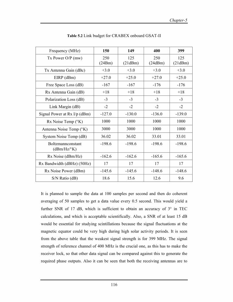
5.7 Link budget

The link budget for the GSAT system is calculated before initiating the final design

of the receiver system and is given in Table 5.2 below. It is seen that as the

transmitter power is very low, a high gain antenna along with a highly sensitive

receiver system is needed to record the received data.

Chapter-5

116

Table 5.2 Link budget for CRABEX onboard GSAT-II

Frequency (MHz) 150 149 400 399

Tx Power O/P (mw) 250 (24Bm)

125 (21dBm)

250 (24dBm)

125 (21dBm)

Tx Antenna Gain (dBc) +3.0 +3.0 +3.0 +3.0

EIRP (dBm) +27.0 +25.0 +27.0 +25.0

Free Space Loss (dB) -167 -167 -176 -176

Rx Antenna Gain (dB) +18 +18 +18 +18

Polarization Loss (dB) -3 -3 -3 -3

Link Margin (dB) -2 -2 -2 -2

Signal Power at Rx I/p (dBm) -127.0 -130.0 -136.0 -139.0

Rx Noise Temp (°K) 1000 1000 1000 1000

Antenna Noise Temp (°K) 3000 3000 1000 1000

System Noise Temp (dB) 36.02 36.02 33.01 33.01

Boltzmannconstant (dBm/Hz/°K)

-198.6 -198.6 -198.6 -198.6

Rx Noise (dBm/Hz) -162.6 -162.6 -165.6 -165.6

Rx Bandwidth (dBHz) (50Hz) 17 17 17 17

Rx Noise Power (dBm) -145.6 -145.6 -148.6 -148.6

S/N Ratio (dB) 18.6 15.6 12.6 9.6

It is planned to sample the data at 100 samples per second and then do coherent

averaging of 50 samples to get a data value every 0.5 second. This would yield a

further SNR of 17 dB, which is sufficient to obtain an accuracy of 3° in TEC

calculations, and which is acceptable scientifically. Also, a SNR of at least 15 dB

would be essential for studying scintillations because the signal fluctuations at the

magnetic equator could be very high during high solar activity periods. It is seen

from the above table that the weakest signal strength is for 399 MHz. The signal

strength of reference channel of 400 MHz is the crucial one, as this has to make the

receiver lock, so that other data signal can be compared against this to generate the

required phase outputs. Also it can be seen that both the receiving antennas are to

Chapter-5

117

have a high gain of 18dB so as to meet the SNR requirements. A parabolic dish and/

or a Yagi antenna are the possible choices for high gain at these frequencies.

5.8 Receiver system design

The design of the receiver system is highly complex as it has to receive very small

signal levels and also need to continuously monitor and record the data. The

following section highlights the design, development and implementation details of

the major subsystems for the receiver, which consists of antennae, outdoor unit,

indoor unit and a PC based data acquisition unit. The block schematic of this is

shown in figure 5.3.

Figure 5.3 Block schematic of ground receiver system

The ground receiver consists of three antennae immediately followed by three

LNAs. The 150 MHz signal is received at the antenna as left circularly polarised

(LCP, ordinary) and right circularly polarised (RCP, extra-ordinary) component and

fed to the dual 150 MHz channels. For 400 MHz received signal, no separation of

the polarisation components is made as the Faraday rotation measurements at UHF

Chapter-5

118

is small. The outputs from the LNAs are then taken to a single outdoor unit

consisting of amplifiers, mixers and filters for all the channels, and which performs

the down conversion to intermediate frequencies of 10.7 MHz, 9.7 MHz, 4.0125

MHz and 3.0125 MHz. This is taken by two long cables to the indoor unit, where

the phase information is extracted from the received signals using Phase Locked

Loops. The UHF carrier and sideband are locked to two PLLs and are taken as the

reference signals. The VHF carrier and sideband are then phase compared with the

corresponding references and the outputs are taken as quadrature signals. For the

measurement of Faraday rotation at VHF, the output from the LCP and RCP of the

antennae are processed separately and compared in another phase detector. Thus

there are four pairs of outputs from the indoor unit. These are

Phase difference between UHFC and VHFC

Phase difference between VHFS and UHFS

Phase difference between VHFLCP and VHFRCP

Amplitude of UHFC and VHFC

These four pairs of data signals are taken through an 8 channel data acquisition card

to PC where a LabVIEW software performs the data acquisition and archival.

5.8.1 Antenna

The first major component of the receiver system is the antenna. Two different types

of antennae were proposed for GSAT beacon reception. The linearly transmitted

signal from the satellite beacon gets polarised because of its propagation through the

ionosphere, and hence in order to study the ionospheric effects at these frequencies,

polarisation reception antennas are preferred at the ground stations as mentioned by

Evans and Cott [1976]. If we have two separate antennae which can receive these

polarized signals separately, it is possible to process these to find out the rotation

undergone by the radio wave. This in turn is proportional to the Faraday rotation as

detailed by George Kennedy [1977], and this can be used to find TEC as detailed in

Chapter 3.

Thus, in the present context, the antennae proposed are

Chapter-5

119

(i) Crossed Yagi array

This requires two separate antennas, one for VHF (149 and 150 MHz) and other for

UHF (399 and 400 MHz). Each of the Yagi elements are of crossed type so as to

receive both the polarisations at the required frequencies. Though it is needed to

separate out LCP and RCP at VHF only, for design compatibility, similar type of

elements are first planned for both. In such a case, a phase matched network is

needed at UHF antenna output, before LNA block. Both the antenna are mounted

parallel along a single boom, so as to maintain phase coherency and reduce pointing

inaccuracies.

(ii) Parabolic dish antenna

Two separate dish antennae are needed, with one having VHF (149 and 150 MHz)

feed and the other having UHF (399 and 400 MHz) feed. The feed is designed to

receive both polarisations separately. Care should be taken in maintaining pointing

accuracies, as two separate structures are required.

A detailed study is done for optimizing the antenna to be selected for this project. It

is seen that a parabolic dish antenna has higher gain and lower beamwidth than a

crossed Yagi. But at the frequencies of reception here, design of a proper feed poses

a challenge for the same dish size. This can be overcome if the dish sizes are made

in proportion to the frequencies of reception. ie, VHF should have a bigger dish size,

which poses an implementation problem. Finally, this resulted in the selection of

antennae as crossed Yagi for VHF and parabolic dish for UHF. The design and

implementation of both these antennas are detailed below.

5.8.1.1 Specifications of Yagi antenna for VHF reception

The following are the finalised specifications for receiving VHF signals using Yagi

antenna.

The co

geome

Using

design

VHF.

increa

Folded

imped

ohms.

imped

param

T

Fre

G

Pola

V

Beam

Ban

onfiguration

etry, both co

Figur

g the softwar

ned for the

The gain of

ase in receiv

d dipoles a

dance transf

. These balu

dance. The

meters.

Table 5

Type

quency

Gain

arisation

VSWR

m width

ndwidth

n of a crosse

onfigured in

re 5.4 Geom

re “Y agicad”

individual e

f the array is

ver sensitivi

are used as

formation ha

uns have bee

following T

1

5.3 Specifica

Crossed Y

ed dipole Ya

the same bo

metry of a cro

”, the follo

elements of

estimated to

ity for all c

s receiving

ave been us

en made of λ

Table 5.4 s

120

ations of Yag

Yagi (one for L

150 MHz,

+13dB

LCP &

1.5 no

10° - 20

2 M

agi antenna h

oom, is show

ossed Yagi (S

owing optim

the Yagi. T

o be ~ 13dB

channels so

element in

sed to obtai

λ/2 coaxial c

shows the f

gi antenna

LCP and one

149 MHz

Bi min

& RCP

minal

0° typ.

MHz

having a hor

wn in figure 5

Source : ARRL

mized config

This array h

, which actu

that signal

n the array.

in an output

cables of 50

finalised Ya

Ch

for RCP)

rizontal and

5.4.

website)

guration ha

has 13 eleme

ually calls fo

ls can be d

. Baluns w

t impedance

ohms charac

agi antenna

hapter-5

vertical

as been

ents for

or ~ 3dB

detected.

with 4:1

e of 50

cteristic

design

Chapter-5

121

Table 5.4 Yagi antenna design parameters for 150MHz

Nomenclature Length (mm) Spacing

R 1075 0

Dp 975 300

D1 965 429

D2 885 671

D3 875 1008

D4 865 1423

D5 859 1907

D6 857 2451

D7 851 3041

D8 845 3678

D9 845 4346

D10 845 5048

D11 841 5774

D12 839 6504

D13 839 7238

Diameter of Boom 75mm

Diameter of element 152 mm

Length of boom 7.2 mtrs

As it is not possible to measure the antenna pattern accurately onsite after

installation, theoretical evaluation is opted here. However, the return loss of the

antenna was measured after installation and each polarization checked separately.

5.8.1.2 Specifications of parabolic dish antenna for UHF reception

The UHF antenna is designed to receive Right Circular Polarized signals (RCP).

Hence the feed is left circularly polarized, as explained by Constantine Balanis

[1982]. A parabolic Aluminium reflector of 24 metre aperture diameter was

refurbished and installed at SPL (TERLS area) for reception of UHF signals. The

Aluminium reflector is chosen as it is non-corrosive and is suitable for use at humid

Chapter-5

122

places. The feed for the dish antenna is the 400 MHz microstrip patch antenna

presently used for LEOs reception.

The air dielectric microstrip antenna is designed to generate circular polarization

without external polarizer arrangements and is found to be the best choice at this

frequency. This type of antenna is mechanically simple, light weight, less complex,

offers less aperture blockage, gives less phase centre errors and can be designed to

meet required amplitude taper requirements with less complex design.

An almost square patch antenna diagonally fed with a single coaxial feed and having

almost the same dimensions as the one used for LEOS reception and given in Table

4.4 is chosen as feed. This antenna has been designed using 3 mm thick Aluminium

sheet for the ground plane and single side copper-clad Hylam sheet of 1.6 mm thick

for the patch. The copper coated side is kept facing down at a height of 10 mm from

ground plane by using Nylon spacers at the four corners of the top plate. The feed

geometry is shown in figure 5.5.

Figure 5.5 Geometry of 400 MHz feed

Chapter-5

123

The elevation plane patterns showed that the gain of the antenna at 65° from the

zenith falls by about 13.5 dB. Assuming an aperture efficiency of 76 %, the

expected gain at 400 MHz for a parabolic reflector of aperture diameter 20 feet (6.1

meter) with the microstrip antenna as feed is given by

GD= (πd/λ0)2* 76% (5.1)

which expressed in dB is

GD dB= 20*log 10 (πd/λ0) -1.2dB =26.9dB (5.2)

where λ0 is the free space wavelength of 400 MHz frequency and D the aperture

diameter of the parabolic reflector.

The detailed specification of the parabolic dish is given in Table 5.5 below.

Table 5.5 Specifications of parabolic antenna

Frequency of operation 400 and 399 MHz

Gain > 18 dBi

VSWR 1.5 nominal

Impedance 50 Ω coaxial

F/D of antenna 0.4 to 0.5

Polarization of feed LCP

A photograph of the feed realized for 400 MHz is shown in figure 5.6.

Figure 5.6 Photo of 400 MHz feed

Chapter-5

124

5.8.2 Outdoor unit

The outdoor unit is mounted at the base of the antenna structure itself and is

hermetically sealed. The signals from the antennae are routed to the outdoor unit

using phase-matched cables as described in Chapter 4. The specifications for the

outdoor unit is given in the table below and block diagram is shown in figure 5.7.

Table 5.6 Specifications of outdoor unit

No. of input ports 3

Input

RCP 1 VHFC, VHF LSB

RCP 2 UHFC, UHFLSB

LCP VHFC, VHFLSB

No. of output ports 2 (RCP & LCP)

Output

RCP 10.7MHz, 9.7MHz, 4.0125MHz,

3.0125MHz

LCP 4.0125MHz

Gain Better than 30 dB for all frequencies

Noise figure 3dB maximum

Bandwidth 2MHz ± 10%

Input and output impedance 50Ω

VSWR 1.5:1

Max. input handling capability +10dBm

Input signal dynamic range 20dB for all channels.

Input signal level -120 to -140dBm

The outdoor unit comprises of LNAs, preamplifiers, Voltage Controlled Crystal

Oscillator (VCXO), frequency multipliers, mixers, amplifiers, power splitters and

power combiners. There are three channels corresponding to UHF, VHFLCP and

VHFRCP. All channels have similar design architecture.

Chapter-5

125

Figure 5.7 Block schematic of GSAT outdoor unit

The front end of each channel is a LNA. Its main function is to amplify extremely

low signals without adding extra noise, thus preserving the required signal to noise

ratio (SNR) of the systems at extremely low power levels. A good LNA has high

gain, low noise figure, good input and output matching and stability at the lowest

possible current drawn from the amplifier as detailed by Lucek and Damen [1999].

The LNA is followed by preamplifier-filter assembly which gives a linear gain of

~30 dB. For the next stage of down-conversion to IF frequencies, the Local

Oscillator (LO) frequencies, 389.332 MHz and 145.9995 MHz, are generated by

multiplying a stable VCXO, of fundamental frequency 48.6665 MHz by 8 and 3.

The LO1 frequency for the VHF chain is 145.9995 MHz and for the UHF chain is

389.332 MHz. As the onboard frequency has a stability of only 5 ppm, the ground

system is designed to take care of this drift in the frequencies by using a VCXO.

Chapter-5

126

The same VCXO is used for converting the 150 MHz signals of both RCP and LCP

channels to obtain the 4.0125 MHz IF so that the difference between RCP and LCP

components is preserved in phase with respect to the receiver input. After down

conversion, the IF frequencies are VHFC : 4.0125 MHz, VHFLSB : 3.0125 MHz,

UHFC : 10.7 MHz and UHFLSB : 9.7 MHz respectively. The RCP and LCP signals

maintain two separate paths throughout the outdoor unit. The bandwidth of all the

post converter output is 2MHz. The coherent oscillators used for the frequency

conversion to IF ensure the phase relationship between the input frequencies and the

output frequencies. The power supply and the VCXO signal for this unit come from

the indoor unit through the output ports (RCP & LCP). The RCP signals are

combined at the output of the outdoor unit and brought out through a single

connector. This helps reduce the number of long cables to the indoor unit, as well as

to maintain the signal integrity.

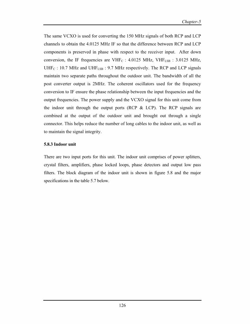
5.8.3 Indoor unit

There are two input ports for this unit. The indoor unit comprises of power splitters,

crystal filters, amplifiers, phase locked loops, phase detectors and output low pass

filters. The block diagram of the indoor unit is shown in figure 5.8 and the major

specifications in the table 5.7 below.

Chapter-5

127

Figure 5.8 Block schematic of GSAT receiver indoor unit

For the modulation phase delay measurement, the 150 MHz carrier and its 1 MHz

side band is brought to the frequencies 4.0125 MHz and 3.0125 MHz respectively,

as also the reference carrier of 400 MHz and its side band to 10.7 MHz and 9.7 MHz

by a phase coherent conversion process employing phase locked loop tracking

filters. Using two separate long loop phase tracking filters, the 150 MHz carrier and

the 400 MHz reference carrier are locked to the stable 48.6665 MHz reference

oscillator. The 1 MHz reference side band on 400 MHz is then reconstructed from

the difference of 10.7 MHz and 9.7 MHz VCXO output using a short loop tracking

filter. The phase difference between the 1.00008 MHz IF output of 150 MHz signal

and the 1.00008 MHz VCXO output of 400 MHz signal gives the 1 MHz

modulation phase delay of 150 MHz signals with respect to the 1 MHz modulation

on 400 MHz. This difference modulation phase is obtained by using the quadrature

components Lc and Ld with the corresponding phase detectors, as shown in the

figure.

Chapter-5

128

For the Faraday rotation measurement, the difference phase is recorded as two

quadrature outputs. This is obtained by multiplying the 4.0125 MHz IF output of the

LCP channel with the 4.0125 MHz reference oscillator signal and its quadrature, La

and Lb in two separate phase detectors. The amplitude of RCP component is the

result of multiplying the signals in phase while the amplitude of LCP component is

the detected output obtained by multiplying out-of-phase signals.

All these outputs are low pass filtered and taken out via a 37 pin connector.

Table 5.7 Specifications of indoor unit

No. of inputs 2 (RCP & LCP)

Input channels RCP 10.7 MHz, 9.7 MHz, 4.0125 MHz, 3.0125 MHz

LCP 4.0125 MHz

No. of outputs 10

Output channels (a) I and Q channels of 4.0125 MHz LCP compared with

4.0125 MHz of RCP

(b) I and Q channels of phase compared 4.0125 MHz of LCP

(c) I and Q channels of phase compared 3.0125 MHz of RCP

(d) Amplitude of 400/ 399 MHz

(e) Amplitude of 150 MHz

(f) Two TTL level signals for both PLLs’ lock.

All the above are provided on a 37pin D type connector.

Input impedance 50Ω

Input VSWR 1.5

Noise figure <4dB

Input signal dynamic range 30dB

Input signal levels -80 to -100dBm

Video bandwidth 40Hz ± 10Hz

5.8.4 Data acquisition unit

The four pairs of signals obtained from the receiver are fed into an 8 channel

simultaneous sampling card SC 2040, where they are sampled simultaneously. The

sampling pulse for this is obtained from the PC through a 68 pin SCSI connector,

Chapter-5

129

which is also connected to a PCI data acquisition card, PCI 6035E, residing in the

PC. This multifunction I/O card has both analog and digital input ports. The analog

signals from the indoor unit are sent to the analog channels and the PLL lock signals

are connected to two digital lines. The start acquisition pulse to SC-2040 is sent

through software from the PC.

The entire data acquisition is controlled by Windows based data acquisition software

developed in LabVIEW which acquires, displays and stores the data samples at the

required sampling rate. The time period and amount of data to be recorded

continuously are determined by this software. The PLL lock signals sensed from the

indoor unit forms the basic criteria to start data acquisition. These are typically TTL

level signals and help to identify whether the PLL is ON/OFF. Though only 10.7

MHz lock signal is used to start acquisition, data from both 10.7 MHz and 1.00008

MHz are logged along with the analog channel data to aid in post processing to

study the temporal variations of the various parameters. The block schematic of the

PC based data acquisition unit is given in figure 5.9, followed by the specifications.

Figure 5.9 Block schematic of data acquisition unit

5.8.5 Data acquisition software

The software for data acquisition is developed in LabVIEW. The main requirements

are :

Simultaneous acquisition of eight analog channels and two digital channels

Chapter-5

130

Start acquisition to be controlled by the state of one digital channel

Provision for manual and automatic stop for data acquisition

Filename to be generated automatically linked with PC date and acquisition

start time.

These functions are implemented using two subVIs - one for data acquisition and the

other for data archival. Both these have a single front panel display. The sampling

rate is kept default as 0.25 Hz, as the changes in GSAT data is expected to be slow.

As there is no Doppler shift involved, the variation detected here can be assumed to

be due to ionosphere only. This chosen sampling rate is kept as a header line in the

raw data file. The software then checks the digital channel corresponding to 10.7

MHz and checks if it is TTL high for at least 1 minute. All the analog data channels

are then acquired, displayed online and saved into eight columns in the data file. The

data file also contains the status of 10.7 MHz PLL and 1.00008 MHz PLL as the last

two columns. For automatic stop of data recording, the TTL pulse has to be low for

a minimum of 5 minutes. This helps to overcome intermittent loss of lock due to any

other strong extraneous signals in the vicinity of the antenna beam. A typical

screenshot of the software front panels during one set of data acquisition is shown in

figure 5.10.

Figure 5.10 Front panels of DAQ software

5.9

Th

wit

lau

5.9

Be

end

Eac

pre

fol

Th

out

pow

an

test

and

ens

As

to r

9 Tests an

e test for the

th signal gen

unch; second

9.1 Integrate

fore the laun

d-to-end. Th

ch of the

ecautions an

lowed here a

e outdoor u

tdoor require

wer supply v

oscilloscop

ted with mu

d range. All

sure phase co

the receiver

reduce man-

Fi

d results

e beacon rec

nerators and

d in the field

ed laborator

nch of satell

he details of

receiver sub

nd initial ca

also.

unit and indo

es a tuning

voltages. A p

e and then

ultiple signal

l these signa

oherency at

r senses very

-made interfe

igure 5.11 B

ceiver was d

d later on wi

test mode w

ry level test

lite beacon, t

all the tests

bunits are

alibration te

oor unit we

DC voltage

pair of outpu

connected

l generators

al generator

the input. T

y low level s

ference.

Block schem

131

done in two

ith the actua

with the beac

ts and result

the entire sy

done are re

tested sepa

ests done d

ere tested in

also from t

uts of the ind

with the DA

in the labor

rs are locked

The laborator

signals, utm

matic of integ

steps, first i

al beacon pa

con in orbit.

ts

ystem is inte

eported in SP

arately and

during LEO

n the integra

the indoor u

door unit wa

AQ unit. T

ratory to che

d to a stable

ry setup is as

ost care is ta

grated test se

in the labora

ayload prior

grated and t

PL Test repo

then integr

OS receiver

ated mode o

unit apart fro

as monitored

he receiver

eck its total

e source in

s shown in fi

aken during

etup in lab

Chapter-5

atory mode

to satellite

tested from

ort [2005].

rated. The

testing is

only as the

om the DC

d first using

system is

sensitivity

the lab to

figure 5.11.

these tests

Chapter-5

132

The indoor unit and outdoor unit are connected with short and long cables during the

tests. The cable losses are also characterised for the desired frequencies. The back

panel indicator of indoor unit is connected to an oscilloscope to check 10.7 MHz and

it is matched with the LED indicator on the front panel when the system is locked to

400 MHz. A detailed test matrix is generated to verify the performance. In order to

check the phase measurement module for measuring Faraday rotation, a mechanical

phase shifter at 150 MHz is introduced before the LNA of RCP channel and the

change in outputs are noted with the phase shifted in steps of 90 degrees.

In the second phase of testing, the receiver system is connected to CRABEX

transmitter directly by providing > 100 dB attenuation to each channel. This

integrated test set up is shown in figure 5.12. As the transmitter power is high

compared to the receiver sensitivity, both the units were kept in different rooms and

long cables were run. Since the receiver has three inputs (two VHF and one UHF),

the VHF output of transmitter was passed through a power splitter after attenuation.

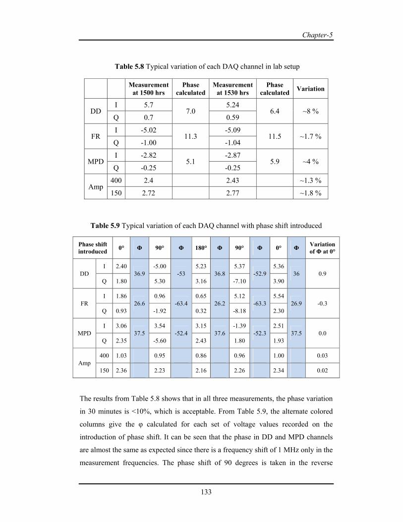
The setup was operated for 30 minutes to check the stability of the transmitter. The

mechanical phase shifter used in the laboratory test was also introduced in one of the

output of the VHF phase splitter and performance evaluated. Some typical results

tabulated are given in Table 5.8 and 5.9.

Figure 5.12 Integrated laboratory test set up with CRABEX transmitter

Chapter-5

133

Table 5.8 Typical variation of each DAQ channel in lab setup

Measurement at 1500 hrs

Phase calculated

Measurement at 1530 hrs

Phase calculated Variation

DD I 5.7

7.0 5.24

6.4 ~8 % Q 0.7 0.59

FR I -5.02

11.3 -5.09

11.5 ~1.7 % Q -1.00 -1.04

MPD I -2.82

5.1 -2.87

5.9 ~4 % Q -0.25 -0.25

Amp 400 2.4 2.43 ~1.3 %

150 2.72 2.77 ~1.8 %

Table 5.9 Typical variation of each DAQ channel with phase shift introduced

Phase shift introduced 0° Φ 90° Φ 180° Φ 90° Φ 0° Φ Variation

of Φ at 0°

DD I 2.40

36.9 -5.00

-53 5.23

36.8 5.37

-52.9 5.36

36 0.9 Q 1.80 5.30 3.16 -7.10 3.90

FR I 1.86

26.6 0.96

-63.4 0.65

26.2 5.12

-63.3 5.54

26.9 -0.3 Q 0.93 -1.92 0.32 -8.18 2.30

MPD I 3.06

37.5 3.54

-52.4 3.15

37.6 -1.39

-52.3 2.51

37.5 0.0 Q 2.35 -5.60 2.43 1.80 1.93

Amp 400 1.03 0.95 0.86 0.96 1.00 0.03

150 2.36 2.23 2.16 2.26 2.34 0.02

The results from Table 5.8 shows that in all three measurements, the phase variation

in 30 minutes is <10%, which is acceptable. From Table 5.9, the alternate colored

columns give the φ calculated for each set of voltage values recorded on the

introduction of phase shift. It can be seen that the phase in DD and MPD channels

are almost the same as expected since there is a frequency shift of 1 MHz only in the

measurement frequencies. The phase shift of 90 degrees is taken in the reverse

Chapter-5

134

direction, so that the calculated phase is negative. Though the tabulated values do

not indicate a system performance for the field tests, it indicates that the receiver

senses the variation in phase. It is also noted that when the system is fully switched

on and off, the initial phase value is always different as has been noted in the case of

LEOS beacon receivers dealt in Chapter 4.

5.9.2 Radiation mode tests and results

In the radiation mode of integrated test with CRABEX beacon, the transmitter

system was switched on from a high rise building few kilometres away and the

integrated ground receiver setup was checked for PLL lock and data acquired. In this

setup, though the antennas were kept in an upright position, the receiver was able to

lock to the beacon transmitter due to its good sensitivity. The data collected during

this mode of tests showed more variations than from the cable mode data given in

Table 5.8 as the signals were transmitted through antenna and a communication

channel and such a change is expected. When the transmitter was switched off, the

receiver went into noise reception and resumed receiver tracking when the

transmitter was switched on again. This ensured the readiness of the ground system

prior to launch. The photograph of Yagi antenna in upright configuration is shown in

figure 5.13.

Chapter-5

135

Figure 5.13 Yagi antennas during radiation mode of test

5.9.3 Field tests and results

After the launch of GSAT-2 in May 2003, the beacon payload was switched on after

about 3 weeks from the launch date, by which time the satellite was parked in a

stable orbit of 255° azimuth and 55° elevation, as viewed by an Indian station. The

first task was then to orient the antenna to point to the satellite and maximise its

signal outputs by adjusting the elevation angle. Both the 400 MHz parabolic dish

antenna and the 150 MHz Yagi antenna were slowly turned to receive the beacon

signal. The test setup during final installation and field tests is diagrammatically

shown in figure 5.14.

Chapter-5

136

Figure 5.14 Field test setup

The antenna was adjusted for the required elevation of 55° and the azimuth was

varied from 210 to 300 to optimize the direction of maximum signal strength, rather

than just fixing at 255°. This signal optimization was done using a spectrum

analyser. The data obtained during optimization of 150 MHz is plotted in figure

5.15. The plot so obtained is also an indirect measure of the antenna radiation

pattern.

Figure 5.15 Signal optimization for Yagi

Both the antennae were locked onto the direction of maximal signal strength. A

photograph of the final configuration of the parabolic dish antenna and Yagi antenna

is shown as figure 5.16.

-124

-123

-122

-121

-120

-119

-118

210 220 230 240 250 260 270 280 290 300

sign

al le

vel

azimuth

150 MHz, 20 points averaged

Chapter-5

137

Figure 5.16 Photograph of the parabolic dish antenna and Yagi antenna

When both the antennae are positioned for maximum signal strength, the received

signal strengths for all the coherent signals are monitored with the spectrum

analyser. The screenshots of the typical signal levels received by the antenna for all

the frequencies as observed with the spectrum analyser is shown in figure 5.17.

Chapter-5

138

Figure 5.17 (a) 400.032 MHz signal Figure 5.17 (b) 399.03192 MHz signal

Figure 5.17 (c) 150.012 MHz signal Figure 5.17 (d) 149.01192 MHz signal

In order to check the signal consistency, continuous monitoring of the signal

strength and frequency shift of the reference channel was done with the same setup,

to ensure that the signal levels are within expected range. The shift in the reference

frequency is an indicator of the shift in all the frequencies as all are coherent and is

the outcome of short term stability of onboard oscillator. Continuous measurements

were done to understand the trend of these variations and some typical plots

generated during these tests are shown in figure 5.18.

Chapter-5

139

Figure 5.18 (a) Variation of UHF frequency over 24 hours

Figure 5.18 (b) Variation of UHF signal strength over 24 hours

Figure 5.18(c) Variation of UHF signal strength over 72 hours

variation of 400.032000 MHz over a day

31800

31900

32000

32100

32200

32300

32400

1200 1545 1930 2315 300 645 1030 1415 1800

time (hrs)

frequ

ency

variation of signal strength over a day

-126

-124

-122

-120

-118

-1161200 1545 1930 2315 300 645 1030 1415 1800

time (hrs)

sign

al le

vel

continuous monitoring of GSAT 400 MHz signal - 72 hours

-107

-105

-103

-101

-99

-971200 1800 0 600 1200 1800 0 600 1200 1800 0 600 1200

time (hrs)

ampl

itude

mea

sure

d in

ana

lyse

r

z

Chapter-5

140

It is seen that under normal circumstances, the signal strength shows a variation of 6

dB and the frequency varies within a range of 400 Hz at 400.032MHz .

The antennas were integrated with the receiver system and continuous data acquired

in the PC. A typical dataset for DD channel with raw data and processed data is

shown in figure 5.19. It can be seen from the phase plot that there is only a small

change in frequency over time, though there is a phase reversal happening between

day and night. This basically implies that there is an enhancement in the electron

density during daytime and a reduction during the night time ionosphere, as has been

reported by various studies including Ramarao et al[2004].

Figure 5.19 (a) Raw data plot of Differential Doppler I, Q and Amplitude channels

(Dated 11.05.2005)

Figure 5.19 (b) Normalized phase plots of raw data showing phase reversal

Chapter-5

141

5.10 Offline processing software and discussion on the results

The GSAT beacon data saved in the file is processed to derive the TEC and

scintillation indices. An offline software is developed in LabVIEW which performs

initial signal processing and saves the processed data onto a file for later scientific

analysis.

The software first separates out the data channels corresponding to each mode of

measurement. The raw data file has the first two columns as the quadrature data

obtained for differential Doppler measurement ie, the phase difference between the

RCP signals of 400 MHz and 150 MHz, measured at the IF of 4.0125 MHz. These

are received as analog channels 0 and 1. These two are separated out first and

normalized to make the total swing to constant amplitude of ±1. It is then passed

through a fifth order Butterworth low pass filter with 1 Hz cutoff frequency and 10

Hz sampling rate, to smoothen out the received signal. The phase is calculated as the

inverse tangent of the ratio of quadrature channel to in-phase channel, followed by

cumulative phase extraction. This is then plotted and saved as secondary data file.

Similar signal processing is done for the other two pairs of data channels, viz, the

phase difference between 1.00008 MHz of 400 MHz and 399 MHz UHF RCP

channels with the 1.00008 MHz of 150 MHz and 149 MHz VHF RCP channels

measured as analog channels 2 and 3 of the DAQ card is processed to give the MPD;

and the phase difference between the 4.0125 MHz of 150 MHz RCP channel with

the 4.0125 MHz of 150 MHz LCP channel corresponding to analog channels 4 and 5

is processed to give the FR data. Each processed data set is saved onto the secondary

file as consecutive columns. The amplitude channels giving the signal strengths of

400 MHz and 150 MHz RCP channels form the 7th and 8th column in the raw data

file, which are normalized and filtered using a 20 mHz fifth order Butterworth low

pass filter to give the amplitude variations.

The front panel of the program with a sample processed data plot is shown in figure

5.20. The continuous variation in DD, MPD and FR are calculated and plotted for

the file chosen for analysis. The ATEC values calculated with the obtained DD and

MPD data is plotted in the second row of the front panel. The PEC plot also shown

Chapter-5

142

in the second row is calculated using ATEC data and FR data. Manju et al [2008]

provides details on importance of this PEC measurement. The last row of plots in

the front panel shows the amplitude variation of 400 MHz received data.

Figure 5.20 Front panel of processing software

All LabVIEW programs give a listing of the modular function calls as VI hierarchy.

The VI hierarchy indicates the number of subVIs and function calls made by the

program when it is run. The major subVIs used here are for phase calculation and

TEC calculation which is shown in figure 5.21.

Figure 5.21 VI Hierarchy of processing software

Chapter-5

143

The variation of Differential Doppler over a day as derived from the data collected is

shown in figure 5.22. The filenames below the plot give the data file details.

Gsat-2-3-06-10-53-29 AM.txt Gsat-2-3-06-7-06-59 PM.txt

Gsat-2-4-06 1-57-31 AM.txt

Figure 5.22 Variation of Differential Doppler data over a day

The above figure shows the cumulative phase variation for a total of almost 24 hours

for the differential phase data. It is seen that there is a gap in the datasets indicating

that more than 5 minutes unlock has been sensed by the DAQ and so the data

recording got automatically stopped. But since the acquisition is in a continuous

loop, the next set of data is acquired once the PLL is locked for more than 1 minute.

This has happened thrice over 24 hours, though the system has recovered within 30

minutes. Now, when the system restarts after a gap, it is also seen that the initial

values in each case is different from the final values of the last plot, which points to

the same uncertainty found with LEOs measurement.

Chapter-5

144

Gsat-2-4-06 1-57-31 AM.txt

Figure 5.23 Variation of phase changes in the three sets of data channels for a

data set

Figure 5.23 above shows the phase variation for all the three methods of TEC

measurement for one typical data file. The phase variation corresponding to absolute

TEC is calculated by summing the corresponding phase values of Differential

Doppler (DD) and Modulation phase delay (MPD) processed data. This is then to be

multiplied by a constant to get ATEC. Similarly, the instantaneous phase values of

the Faraday rotation (FR) channel data is subtracted from this summed value to

obtain the phase variation corresponding to Plasmaspheric Electron content (PEC).

It can be seen that the phase changes of FR and DD datasets follow the same trend,

while the MPD phase remains almost constant. Thus this MPD value gives the

coarse variation of ATEC while DD phase gives the fine variation of ATEC. Also, it

is known that the FR data gives the ionospheric electron content (IEC) upto a

maximum of 2000 km as mentioned by Ramarao et al [2004]. It is also known that

the extent of Earth’s ionosphere can be approximated upto this height, so that the

phase changes indicated by DD phase data and FR phase data can be similar. The

Chapter-5

145

MPD phase variation helps to address the 2nπ ambiguity associated with the LEO

beacon measurements, providing the initial phase value and its trend.

In the scenario of GSAT-II data reception, it is seen that as the signal strength is

very low, any extraneous noise could trigger unlock. In addition, the short term

stability of the onboard oscillator also sets an intricate arrangement, so that the

problem of absolute TEC measurement is not fully addressed. The main sources of

error in converting observations of the Faraday rotation angle of a signal from a

geostationary satellite into total electron content (NT) are the uncertainties in the

baseline corresponding to initial polarisation and in the total number of rotations, ie,

the nπ ambiguity.

5.11 Simulation of an Orthogonal Coded Spread Spectrum beacon

system

A spread spectrum beacon transmitter in a geostationary orbit can address the

uncertainty measurement of absolute TEC. In the earlier chapter, simulation of one

method for phase measurement by transmitting dual coherent frequencies has been

described. Yet another approach is to assign a unique set of spreading sequences to

each frequency in a multicarrier DS-CDMA system. Each of the sequences assigned

to a carrier is distinct. These sequences are selected to be mutually orthogonal (MO)

complementary sequences which help eliminate multiple-access interference (MAI)

in the ideal phase coherent channel, when compared to systems employing a single

spreading sequence to each carrier. The major difference with a normal direct

sequence system is that this system is not as resistant to frequency-selective fading.

However, the system appears well suited to certain types of communication

channels, such as fiber optical channels, which are relatively stable phase-coherent

channels, or Rician channels with a strong line-of-sight (LOS) path, where the

effects of frequency-selective fading are minimal.

In this chapter, a simulation technique for quadrature carrier DS-CDMA that

employs a set of spreading sequences for each carrier is attempted. De-spreading in

the receiver is accomplished on a carrier-by-carrier basis using a set of matched

filters matched to the spreading sequences applied to the respective carriers. Hence,

Chapter-5

146

excluding MAI and noise, the output of the matched filter corresponding to a

particular carrier channel is just the autocorrelation function of the corresponding

spreading sequence. This technique has been used with CDMA systems in wireless

and mobile communications as described in the patent of Lattard et al [1998] with

multiple carriers to enhance channel capacity and data rate.

The broad functional schematic of the simulation software is shown in figure 5.24.

Each of the code and carrier subVIs and modules are similar to the ones explained in

Chapter 4.

Figure 5.24 (a) Functional schematic of OCSS transmitter simulator

Figure 5.24 (b) Functional schematic of OCSS receiver simulator

The system consists of a transmitter block, propagation channel block and the

receiver block. A coherent signal source with in-phase and quadrature outputs forms

the first block. For generation of two different PN codes, a separate subVI is

developed, which give maximum cross-correlation. The communication channel is

modelled here as a Rician fading channel, instead of Rayleigh channel used in the

Chapter-5

147

earlier simulation. The exact channel model depends on various parameters like the

orbit type, atmospheric effects, and terrain and elevation angle as has been detailed

in various earlier works like Derek A Wells [2003], Trintinalia and Casillo [2006]

and Ali Arsal [2008]. The present configuration of a geostationary system is suitable

for study of small-scale variations. In such a randomly varying small-scale channel,

the distribution of received signal power or envelope dramatically affects the

performance of a receiver. These fluctuations are best described using a probability

density function (PDF), which characterizes all of the first-order statistics of a

channel as explained by Gregory D. Durgin [2002]. This PDF was originally

formulated for characterizing temporal fading measurements from upper-atmosphere

propagation. A typical distribution is shown in figure 5.25.

Figure 5.25 PDF of different communication channels

Thus for the present simulation, the Rician function is chosen, which can be

effectively represented as phase delay function in software. This can contribute for a

phase change in the carrier and code in addition to reducing the signal strengths.

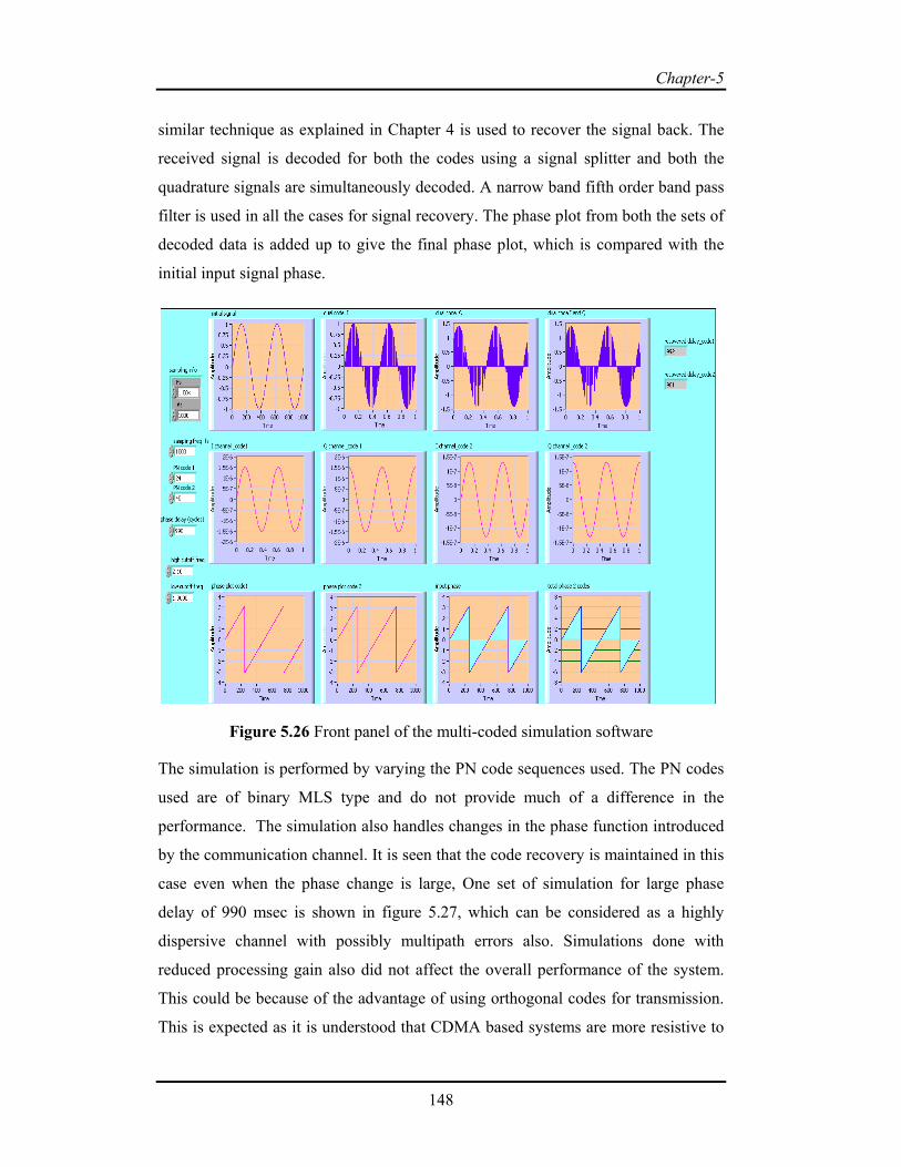
The front panel of the simulation software for the multi-code modulation is shown in

figure 5.26 below. In this, two codes are used to modulate a quadrature carrier. The

input signal followed by modulation by a single PN sequence is shown first, and

then modulated by the second code and added with the first to give the final

transmitter signal. This passes through a Rician distributed channel, which produces

a phase shift in the transmitted signal in addition to adding noise. In the receiver, a

Chapter-5

148

similar technique as explained in Chapter 4 is used to recover the signal back. The

received signal is decoded for both the codes using a signal splitter and both the

quadrature signals are simultaneously decoded. A narrow band fifth order band pass

filter is used in all the cases for signal recovery. The phase plot from both the sets of

decoded data is added up to give the final phase plot, which is compared with the

initial input signal phase.

Figure 5.26 Front panel of the multi-coded simulation software

The simulation is performed by varying the PN code sequences used. The PN codes

used are of binary MLS type and do not provide much of a difference in the

performance. The simulation also handles changes in the phase function introduced

by the communication channel. It is seen that the code recovery is maintained in this

case even when the phase change is large, One set of simulation for large phase

delay of 990 msec is shown in figure 5.27, which can be considered as a highly

dispersive channel with possibly multipath errors also. Simulations done with

reduced processing gain also did not affect the overall performance of the system.

This could be because of the advantage of using orthogonal codes for transmission.

This is expected as it is understood that CDMA based systems are more resistive to

Chapter-5

149

channel fading and multipath, both of which can be represented by noise and phase

shift in the traversing signal.

Figure 5.27 Dual PN code modulating quadrature carrier in a dispersive channel

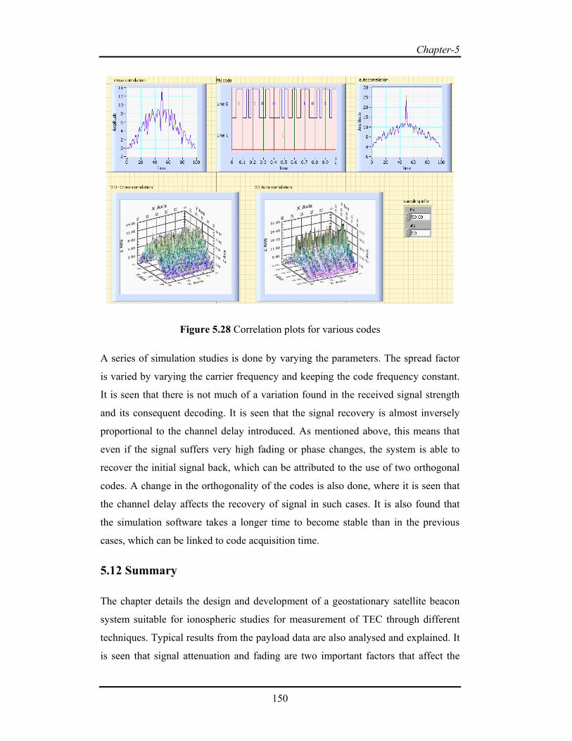
The autocorrelation and cross-correlation properties of the different PN codes used

in this simulation are plotted as a 3D graph in figure 5.28. The autocorrelation and

cross-correlation of two typical codes are also shown along with a digital

implementation of one PN signal.

Chapter-5

150

Figure 5.28 Correlation plots for various codes

A series of simulation studies is done by varying the parameters. The spread factor

is varied by varying the carrier frequency and keeping the code frequency constant.

It is seen that there is not much of a variation found in the received signal strength

and its consequent decoding. It is seen that the signal recovery is almost inversely

proportional to the channel delay introduced. As mentioned above, this means that

even if the signal suffers very high fading or phase changes, the system is able to

recover the initial signal back, which can be attributed to the use of two orthogonal

codes. A change in the orthogonality of the codes is also done, where it is seen that

the channel delay affects the recovery of signal in such cases. It is also found that

the simulation software takes a longer time to become stable than in the previous

cases, which can be linked to code acquisition time.

5.12 Summary

The chapter details the design and development of a geostationary satellite beacon

system suitable for ionospheric studies for measurement of TEC through different

techniques. Typical results from the payload data are also analysed and explained. It

is seen that signal attenuation and fading are two important factors that affect the

Chapter-5

151

ground reception of these signals. In order to address this, usage of a spread

spectrum modulated beacon in a geostationary orbit is proposed and simulation

studies using quadrature carrier CDMA techniques is explored, using LabVIEW. It

is seen that in these cases, usage of orthogonal codes for the carrier modulation

increases the fading margin and the signal can be recovered fast and thus it provides

an advantage over the existing beacon system.