Development of a flow-condition-based

interpolation 9-node element for incompressibleflows

by

Bahareh Banijamali

Submitted to the Department of Civil and Environmental Engineeringin partial fulfillment of the requirements for the degree of MA

Doctor of Philosophy in Structures and MaterialsMAR 0 9 2006

at the

MASSACHUSETTS INSTITUTE OF TECHNOLOGY LIBRARIES

February 2006

( Massachusetts Institute of Technology 2006. All rights reserved.

1 /

A uthor .. . . .. . .. .. ... . ....... .... .. ........

Depart enCivil and Environmental EngineeringAugust 23, 2005

Certified by .........................................................Klaus-Jiirgen Bathe

Professor of Mechanical EngineeringThesis Supervisor

C ertified by ...... .. ..................... ......................Franz-Josef Ulm

Associate Professor of Civil and Environmental Engineering-, I~) Tlhesis Supervisor

Accepted by ...................... ;. .............Andrew J. Whittle

Chairperson, Department Committee on Graduate Students

ARCHIVES

2

Development of a flow-condition-based interpolation 9-node

element for incompressible flows

by

Bahareh Banijamali

Submitted to the Department of Civil and Environmental Engineeringon August 23, 2005, in partial fulfillment of the

requirements for the degree ofDoctor of Philosophy in Structures and Materials

AbstractThe Navier-Stokes equations are widely used for the analysis of incompressible lami-nar flows. If the Reynolds number is increased to certain values, oscillations appearin the finite element solution of the Navier-Stokes equations. In order to solve forhigh Reynolds number flows and avoid the oscillations, one technique is to use theflow condition-based interpolation scheme (FCBI), which is a hybrid of the finiteelement and the finite volume methods and introduces some upwinding into the lam-inar Navier-Stokes equations by using the exact solution of the advection-diffusionequation in the trial functions in the advection term.

The previous works on the FCBI procedure include the development of a 4-nodeelement and a 9-node element consisting of four 4-node sub-elements. In this thesis,the stability, the accuracy and the rate of convergence of the already published FCBIschemes is studied. In addition, a new FCBI 9-node element is proposed that obtainsmore accurate solutions than the earlier proposed FCBI elements. The new 9-nodeelement does not obtain the solution as accurate as the Galerkin 9-node elements butthe solution is stable for much higher Reynolds numbers (than the Galerkin 9-nodeelements), and accurate enough to be used to find the structural responses in fluidflow structural interaction problems.

The Cubic-Interpolated Pseudo-particle (CIP) scheme is a very stable finite dif-ference technique that can solve generalized hyperbolic equations with 3rd order ac-curacy in space. In this thesis, in order to solve the Navier-Stokes equations, theCIP scheme is linked to the finite element method (CIP-FEM) and the FCBI scheme(CIP-FCBI). From the numerical results, the CIP-FEM and the CIP-FCBI meth-ods appear to predict the solution more accurate than the traditional finite elementmethod and t;he FCBI scheme. In order to obtain accurate solutions for high Reynoldsnumber flows, we require a finer mesh for the finite element and the FCBI methodsthan for the CIP-FEM and the CIP-FCBI methods. Linking the CIP method to thefinite element and the FCBI methods improves the accuracy for the velocities andthe derivatives. In addition, when the flow is not at the steady state and the timedependent terms need to be included in the Navier-Stokes equations, or in the prob-

lems when the derivatives of the velocities need to be obtained to high accuracy, theCIP-FCBI method is more convenient than the FCBI scheme.

Thesis Supervisor: Klaus-Jiirgen BatheTitle: Professor of Mechanical Engineering

Thesis Supervisor: Franz-Josef UlmTitle: Associate Professor of Civil and Environmental Engineering

Acknowledgments

When I was offered a four year position as a Ph.D. student at MIT, I had only heard

of the place. I barely thought I would go to MIT one day or spend four years of my life

getting Ph.D. and being away from my family and my good friends. Assured by many

that this was an opportunity that should not be missed, I left home and my loved

ones. Now I realize that I have been extraordinarily lucky to have spent the last four

years at MIrT. There are so many wonderful things that could be said about MIT;

the people, the lack of hierarchy, the open doors, the never-ending conversations,

the atmosphere, the many workshops, countless interesting visitors and the diversity

of interests. It is hard to imagine a more stimulating and encouraging academic

environment. It will be difficult and sad to leave.

I am not leaving MIT only with the Ph.D. degree but with lots of memories and

experiences. Memories of extremely stressful situations and memories of intense joy.

I remember times I had wished to be away from MIT just to be able to be relax

and sleep without being worried about my research, and times I had appreciated the

chance of being a student at MIT. Needless to say that I could not have come so far if

it were not for all the people that were near me, supported me, gave me strength and

helped me to be patient and strong. During these four years, I have been fortunate

to interact with many people who have influenced me greatly. One of the pleasures

of finally finishing is this opportunity to thank them. I am sure I will not be able to

include all of them, but at least let me mention the people that had most influenced

my life during these four years.

First of all I would like to thank Prof. Klaus-Jfirgen Bathe, my thesis advisor, who

guided me through the world of research and supported me during the development of

this research work. He gave me the opportunity to explore the world of finite element

methods. His ability to rapidly assess the worth of ideas and algorithms is amazing. I

would spend a week or two on an approach to a problem and Bathe could understand

it, reconstruct it and tell me (correctly) that it would not work in about a minute.

I would also want to thank the members of my Thesis Committee, Prof. Jerome J.

Connor and Prof Franz-Josef Ulm. I am particularly grateful to Prof. Connor. He is

one of the people I will always respect and remember for his kind heart and the way

he cares and supports all the students. In addition, I am thankful to Prof. Eduardo

Kausel for always smiling and giving me support and encouragement whenever I was

seeing him in the hallways or CEE events. I am also grateful to the researchers of

ADINA R&D for their support with the use of ADINA.

I would also like to thank the people of the Finite Element Research Group at

MIT (my lab-mates) Irfan Baig, Phill-Seung Lee, Junh-Wuk Hong, Jacques Olivier,

Thomas Gretsch, Francisco Montans and Haruhiko Kono for their daily conversations

and their friendship. Irfan, in particular, since we were the only two people in the

lab during the last year of my thesis and he was always willing to talk with me and

to give me advice and supportive comments.

I have made many friends along the way. Friends from different worlds and differ-

ent cultures, people from each I learnt many new things. They have helped me, one

way or another, in my struggle to complete my Ph.D. and my thesis. Many thanks to

Farinaz Edalat, Taraneh Parvar, Maryam Modir Shanechi, Behnam Jafarpour, Sheila

Tandon, Nima Shokrollahi and Elwin C Ong. In addition, many thanks to my friends

back home, Mandana Bejanpour, Alireza Gharagozloo, Amir Maleki, Sanaz Khalili

and Saharnaz Bigdeli and my cousin Soheila Chitsaz, who constantly loved me, sup-

ported me and gave me courage and strength during the four years of my Ph.D. at

MIT.

I would also like to thank Blanche E Staton, Lynn Roberson and all the girls in the

Graduate Women Group and Graduate Women Group in Civil Engineering depart-

ment for their encouragement and support, and for providing a friendly atmosphere

in the "Graduate Women Lounge". We spent many afternoons studying together or

discussing our problems and sharing our experiences.

Cynthia Stewart, the academic administrator, is one of the many extremely com-

petent people working at CEE department at MIT. The ongoing health of the CEE

is, I believe, largely due to Cynthia's vision of what CEE and MIT should be, to her

refusal to allow that vision to be compromised, to her warm and friendly personality,

and to her ability to deal calmly and rationally with any situation. She is fortunate

to be surrounded by a team of people who combine to make CEE the unique place

that it is. Jeanette Marchocki is one of them. Many many thanks to Cynthia and

Jeanette to make me feel MIT was my home and I had a family here! I am also

grateful to Una Sheehan, Deborah Alibrandi and Joan McCusker for always listening

to me when I needed to talk, giving me hope and supporting me.

I would also like to thank my fiance and my best friend Yazdan. His support,

encouragement, and companionship has turned the last year of my journey through

Ph.D. into a pleasure. We proved that distance cannot, and will not hurt a bond

between two people that is based on mutual respect, trust, commitment, and love.

We believed that love and relationships are what make life special, and that ones

built on love and understanding are always worth preserving, regardless of the miles

that may separate two people.

It is not possible to summarize Bita, my sister, and her influence on me in one

paragraph, but I will try. Bita has completely encouraged me and supported me over

the last four years. Her love, intelligence, honesty, goodness, liveliness and kindness

have given me strength and patience. She is the most caring person I have ever

known. The fact of her existence is a continual miracle to me. She has supported me

in hundreds of ways throughout the development and writing of this thesis.

Finally, my infinite gratitude goes to my parents, my best friends, for their love

and encouragement and for always showing me the light at the end of the tunnel and

giving meaning to my life. They have given their unconditional support, knowing

that doing so contributed greatly to my absence these last four years. They were

strong enough to let me go easily, to believe in me, and to let slip away all those years

during which we could have been geographically closer and undoubtedly loving living

together. Mom and dad, I love you, I am extremely grateful to what you have done

for me and I am here because of you!

8

Contents

1 Introduction 15

2 Governing equations of continua 21

2.1 Eulerian formulation ........................... 22

2.2 Conservation equations .......................... 23

2.2.1 Mass conservation ........................ 24

2.2.2 Momentum conservation ................... .. 25

2.3 Equations of motion ........................... 26

3 Finite element formulation 29

4 Flow-condition-based interpolation scheme (FCBI) 35

4.1 The governing equations ......................... 36

4.2 The fluid flow discretization ....................... 38

4.3 Fundamental properties of the FCBI procedure . ........... 51

4.4 Numerical examples ............................ 53

4.4.1 The driven cavity flow problem ................. 53

4.4.'2 The S-channel flow problem ................... 59

4.5 Further study of the FCBI scheme . . . . . . . . . . . . . . . . . 64

4.5.1 Stability of the FCBI scheme .................. 64

4.5.2 Accuracy of the FCBI scheme .................. 69

5 A new FCBI 9-node element 79

5.1 Fluid flow discretization ......................... 81

9

5.2 Comparison of the new 9-node element with the earlier published 9-

node element . . . . . . . . . . . . . . . . . . . . . . . ...... 92

5.3 Comparison of the new 9-node element with the Galerkin 9-node element 97

6 Linking FCBI to CIP method (CIP-FCBI)

6.1 CIP method ..........................

6.1.1 One-dimensional CIP solver .............

6.1.2 Two-dimensional CIP solver.

6.1.3 The CIP solver for compressible and incompressible

6.2 Lin:ling the finite element method to the CIP method . . .

6.2.1 The governing equations ...............

6.2.2 Numerical solutions .

6.3 Linking the FCBI scheme to the CIP method .......

6.3.:1 The governing equations ...............

6.3.2 Numerical solutions .

107

...... . 108

...... .109

...... . 115flows . . . 119

. . . ... . . 123

. . . ... .. 123

. . . ... ... 131

...... . 136

. . . ... .. 136

. . . ... . . 145

1517 Conclusions

A Consistency of the CIP scheme

B Stability of the CIP scheme

155

161

10

List of Figures

2-1 Reference, spatial and mesh configurations . ........ 23

4-1 The two-dimensional incompressible fluid flow problem considered . . 37

4-2 9-node elements and a sub-element in isoparametric coordinates . . . 39

4-3 The demonstration of xl and 1 - x1 functions for the flux through ab

for the three different values of ql = 10, ql = 0 and ql = 200 ..... 42

4-4 (a) The driven cavity flow problem (b) The uniform mesh of 8x8 ele-

ments used ................................ 54

4-5 Schematics of solutions for the driven cavity flow problem ...... 55

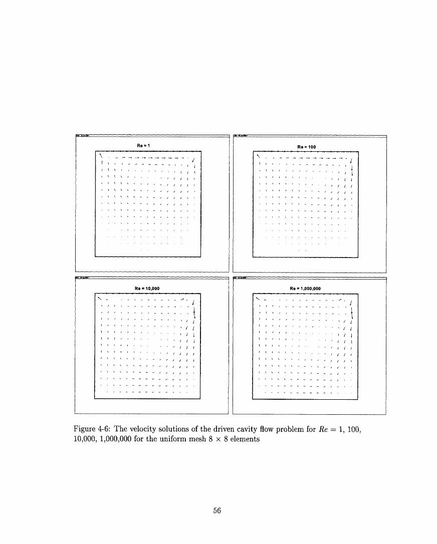
4-6 The velocity solutions of the driven cavity flow problem for Re = 1,

100, 10,000, 1,000,000 for the uniform mesh 8 x 8 elements ..... 56

4-7 The pressure solutions of the driven cavity flow problem for Re = 1,

100, 10,000, 1,000,000 for the uniform mesh 8 x 8 elements ..... 57

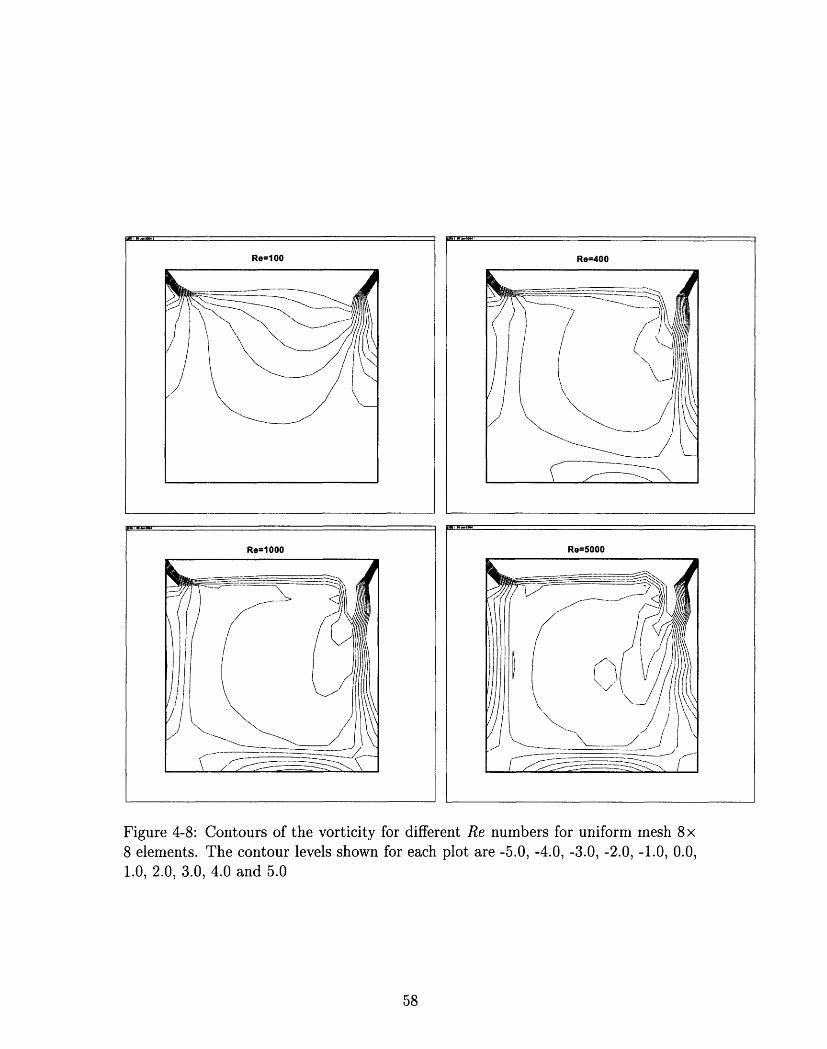
4-8 Contours of the vorticity for different Re numbers for uniform mesh

8x 8 elements. The contour levels shown for each plot are -5.0, -4.0,

-3.0, -2.0, -1.0, 0.0, 1.0, 2.0, 3.0, 4.0 and 5.0............... 58

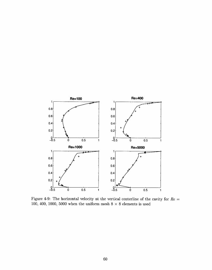
4-9 The horizontal velocity at the vertical centerline of the cavity for Re

= 100, 400, 1000, 5000 when the uniform mesh 8 x 8 elements is used 60

4-10 The vertical velocity at the horizontal centerline of the cavity for Re

- 100, 400, 1000, 5000 when the uniform mesh 8x 8 elements is used 61

4-11 (a) The S-channel flow problem (b) The mesh used .......... 62

4-12 Schematics of solutions for the S-channel flow problem (a) Re = 100,

(b) Re = 10,000 .............................. 63

11

4-13 The velocity solutions of the S-channel flow problem for Re = 1, 100, 10,000

for the mesh shown in figure 4-11 (b) .................. 65

4-14 The pressure solutions of the S-channel flow problem for Re = 1, 100, 10,000

for the mesh shown in figure 4-11 (b) .................. 66

4-15 Pressure solutions obtained by the FCBI procedure using the mesh

shown in Fig. 4-11(b) and the two times finer and coarser meshes when

Re := 100 ................................. 67

4-16 Pressure solutions obtained by the ADINA program using the mesh

shown in Fig. 4-11(b) and the two times finer mesh when Re = 100 68

4-17 The non-uniform mesh of 4x4 9-node elements used .......... 73

4-18 Comparison of the FCBI 9-node elements, FCBI 4-node elements and

the Galerkin 9-node elements for the driven cavity flow problem (Re=1000).

In this figure, the x coordinate represents log h when h is the ele-

mert size and the y coordinate for each case is a) log Ilu-UhIlL2 b)IIUIIL2'

log lU-Uhll H c) log P112 , d) lg ( U-UhIIH1 IPII-PhL2 ).

4-19 Comparison of the FCBI 9-node elements, FCBI 4-node elements and

the Galerkin 9-node elements for the S-channel flow problem (Re=100).

In this figure, the x coordinate represents log h when h is the ele-

merit size and the y coordinate for each case is a) log I lu-uhIL2 b)

log |u-u||H 11. c) log iPPhiL2 , d) log ( UhIIH1 + IPPhIIL2 ).77[[UI[H 1 , IIPIL2 IIUIIHi liP1l2

5-1 The new FCBI 9-node element (a) The element in its isoparametric

coordinates, (b) Definition of Axk for the flux through 5-7 ...... 82

5-2 The demonstration of f, g and 0 functions for the flux through 5-7 for

the three different values of ql = 10, q2 = 0 and q3 = 200 ....... 85

5-3 The trial functions hI, h and h for the flux through 5-7 ....... 87

5-4 The earlier proposed 9-node element (consists of four 4-node sub-

elements); x1 and (1 - xzl ) functions are shown for one sub-element

and the assemblage of two adjacent sub-elements for high Reynolds

number flow when the flux is through 5-7 ................ 89

12

5-5 Illustration of Q., and Qq; the control volumes of the velocity and

pressure points respectively ....................... 92

5-6 Comparison of the new FCBI 9-node elements and the original FCBI

9-node elements for the driven cavity flow problem (Re=1000). In this

figure, the x coordinate represents log h when h is the mesh size and

the y coordinate for each case is a) log IUUhIlL2 , b) log ,lu-uhlHl, c)IUlIL IIUIIH1

log IP-PhiL2 , d) log (11u-uhllH + -Ph ). . . . . . . . . . . . . 96[[p[[L 2 '[U[[H 1 [[P[[L

2

5-7 Comparison of the new FCBI 9-node elements and the original FCBI

9-node elements for the S-channel flow problem (Re=100). In this

figure, the x coordinate represents log h when h is the mesh size and

the y coordinate for each case is a) log IIU-UhL2 , b) log IluhJIHl , c)IIUHIL2 IIUIIH1

log IP-PhIL2 , d) log (u-uhH1 + IIP-PhL2 ). . . . . . . 99IIPIIL2 IIUIIH1 - ipiL 2

5-8 Comparison of the new FCBI 9-node elements and the Galerkin 9-node

elements for the driven cavity flow problem (Re=1000). In this figure,

the x coordinate represents log h when h is the mesh size and the

y coordinate for each case is a) log IIU-UhIL2 , b) log Ilu-hllH , c)[UIIL2 ' UIIH1

log 1P-PhjjL2 , d) log (u-UhH1 + ) . . . . . . . . . . . . . 102liPlL2 ' IPH1 P llpPL2

5-9 Comparison of the new FCBI 9-node elements and the Galerkin 9-node

elements for the S-channel flow problem (Re=100). In this figure, the x

coordinate represents log h when h is the mesh size and the y coordinate

for each case is a) log IuulL2 , b) log lu hHll , c) log I-PhiL2 d)11ulIL2 'IuIll1 )liPlL2

6-1 The principle of the CIP method. (a) The initial profile and the exact

solution (b) The exact solution at the grid points (c) Linear profile

between the grid points (d) The spatial derivative in the CIP method 110

6-2 The 4-node element used in the finite element discretization ..... 127

6-3 The driven cavity flow problem . .................... 131

6-4 The non-uniform meshes used for (a) Re = 1000, (b) Re = 10000. .. 133

6-5 Velocity profiles for Re = 1000. ..................... .. 134

13

6-6 Velocity profiles for Re = 10000 ...................... 135

6-7 9-node elements and the 4-node sub-element used in the finite element

discretization ............................... 139

6-8 The non-uniform meshes used for (a) Re = 1000, (b) Re = 10000. .. 147

6-9 Velocity profiles for Re = 1000. ...................... 148

6-10 Velocity profiles for Re = 10000 ...................... 150

14

Chapter 1

Introduction

The study of incompressible flows is important in many areas of science and tech-

nology. At low speeds the flow will be ordered and follow regular patterns, i.e., it

is laminar flow. Common applications in which laminar flow appears are biological

fluid flow, Newtonian flows in chemical and mechanical engineering and any indus-

trial process involving heat, fluid flow and mass transport at low Reynolds numbers.

A balance between the inertia and viscous forces governs laminar flows and provides

the stability. Flows are often characterized by a dimensionless number known as the

Reynolds number, which is the ratio of inertia to viscous forces in a flow. Laminar

flows correspond to smaller Reynolds numbers. Even though laminar flows are deter-

ministic and ordered, instabilities and bifurcation may happen in the flow and take

the flow from being laminar to be transition or turbulent. Numerical modelling of

transition and turbulence requires greater insight into the flow physics.

For higher Reynolds numbers, the flow is governed by inertial forces and in most

cases of engineering problems the flow is in a disordered or turbulent state. Common

applications of incompressible turbulent flows involve the flow around vehicles and

low speed flows in aeronautics where the fuel efficiency is greatly impacted by the

details of the flow.

The Navier-Stokes equations are widely used for the analysis of incompressible

laminar flows. If the Reynolds number is increased to certain values, oscillations

appear in the finite element solution of the Navier-Stokes equations. In order to

15

solve for high Reynolds number flows and avoid the oscillations, one technique is to

use stabilized methods. In these methods, artificial upwinding is introduced into the

equations to stabilize the convective term, ideally without degrading the accuracy of

the solution: e.g. the streamline upwind/Petrov-Galerkin (SUPG) method [7], the

Galerkin/least-squares (GLS) method [15], the Cubic Interpolated Pseudo/Propagation

(CIP) method [27] and use of the bubble functions [10], [6], [5], [22].

The flow condition-based interpolation scheme (FCBI) is a hybrid of the finite

element and the finite volume methods and it was first introduced by KJ. Bathe and

J. Pontaza in [2]. This scheme was later developed in [3], [19] and [20].

The FCBI procedure introduces some upwinding into the laminar Navier-Stokes

equations by using the exact solution of the advection-diffusion equation in the trial

functions in the advection term. The FCBI procedure is a finite element method since

the domain of the problem is considered as an assemblage of discrete finite elements

connected at nodal points on the element boundaries, and the velocity and the pres-

sure are interpolated within each element. This procedure can also be considered a

finite volume method since the weak form of the Navier-Stokes equations is satisfied

over control volumes, when the test functions are unit step functions. Hence, the

FCBI finite element solution satisfies the mass and momentum conservations for the

control volumes (the traditional finite element methods do not satisfy the local mass

and momentum conservations).

One reason why the FCBI procedure was proposed as a hybrid of the finite element

and the finite volume methods, not being merely a finite volume method, is the

lack of defining interpolation functions in the finite volume methods. Defining the

interpolation functions enables us to directly evaluate the derivatives, and set up the

Jacobian matrix for the Newton-Raphson iteration method. Also, no artificial factors

are used and similar to the traditional finite element methods a mathematical theory

is available.

The basic aim in developing an FCBI scheme is to reach a numerical scheme that

is stable for low and high Reynolds numbers, and yields sufficiently accurate solutions

using coarse meshes. Of course, the numerical solution of the laminar Navier-Stokes

16

equations at; high Reynolds numbers would not be highly accurate. The fluid mesh

would need to be too fine. However, when a coarse mesh is used, the scheme should

still yield a reasonable solution. As the mesh is then refined, the numerical scheme

would capture more details in the flow; e.g. circulations, and the solution obtained

would ideally converge to the exact solution of the mathematical model. At some

stages of the mesh refinement, a turbulent model might be required.

However., in practice, the accuracy of the solution and the computational cost are

important issues. These issues are particularly important in the analysis of the fluid

flows with structural interactions.

The analysis of fluid flows with structural interactions has captured much attention

during the recent years. Such analysis is performed considering the solution of the

Navier-Stokes fluid flows fully coupled to the non-linear structural response. However,

a fully coupled fluid flow structural interaction analysis can be computationally very

expensive. The cost of the solution is, roughly, proportional to the number of nodes

or grid points used to discretize the fluid and the structure.

In order for interaction effects to be significant, the structure is usually thin and

can be represented as a shell, hence not too many grid points are required. The large

number of grid points and consequently number of equations in fluid flow structural

interaction problems (FSI) is due to the representation of the fluid domain. For high

Reynolds number fluid flows, to have a stable solution, more grid points are required.

In order to decrease the number of grid points in the fluids (using a coarser mesh) and

still have a stable solution, the flow-condition-based interpolation (FCBI) procedure

was introduced [2], [3], [4].

The basic philosophy of FCBI scheme was presented earlier in [2]. However,

our aim is to increase the effectiveness of this scheme. The previous works on the

FCBI procedure include the development of a 4-node element and a 9-node element

consisting of four 4-node sub-elements. In this thesis, the stability, the accuracy and

the rate of convergence of the already published FCBI schemes is studied in section

4.5, and it is shown that the FCBI 4-node elements and the earlier proposed FCBI 9-

node elements obtain more stable solutions than the Galerkin 9-node elements, used

17

in the traditional finite element methods. However, the Galerkin 9-node elements

give more accurate solutions with a higher rate of convergence. Our objective is

to use the FCBI scheme in rather coarse meshes together with the "goal-oriented

error measurements" technique to control error in the structural response in the fluid

flow structural interaction problems [12]. Hence, in chapter 5 we propose a new

FCBI 9-node element that obtains more accurate solutions than the earlier proposed

FCBI elements. The new 9-node element does not obtain the solution as accurate

as the Galerkin 9-node elements but the solution is stable for much higher Reynolds

numbers (than the Galerkin 9-node elements), and accurate enough to be used to find

the structural responses.

In chapter 6, the focus is on the Cubic-Interpolated Pseudo-particle (CIP) method.

The CIP method was introduced by T.Yabe et al. in 1991 [26], [17] . In this method,

a cubic polynomial is used to interpolate spatial profiles and spatial derivatives. The

spatial derivative itself is a free parameter and satisfies the master equation for the

derivative. After the values have been found, the same values for the next time step

are simply calculated by shifting the cubic polynomial.

The CIP scheme is a very stable finite difference technique that can solve gener-

alized hyperbolic equations with 3rd order accuracy in space. In this thesis, in order

to solve the Navier-Stokes equations, the CIP scheme is linked to the finite element

method (CIF'-FEM) and the FCBI scheme (CIP-FCBI).

The thesis is organized as follows. In Chapter 2 a brief review of the contin-

uum governing equations for fluid flows is given, which includes the definition of

the Eulerian formulation, the conservation equations and the equations of motion.

Chapter 3 describes the finite element discretization of those governing equations.

Chapter 4 is devoted to the introduction of the FCBI procedure, the discretization

of the FCBI scheme for the earlier proposed 9-node elements (consisting of four 4-

node sub-elements), the solution of some numerical examples and a further study

of the FCBI scheme for these elements. Subsequently, in Chapter 5, a new FCBI

9-node element is proposed and compared with the former FCBI 9-node element and

the Galerkin 9-node element. In Chapter 6, a review of the CIP method is given.

18

Then, in order to solve the Navier-Stokes equations, the CIP scheme is linked to the

finite element method (CIP-FEM) and the FCBI scheme (CIP-FCBI) respectively.

Finally, in Chapter 7 the conclusions of this work are given and future research in the

development of the FCBI scheme is suggested.

19

20

Chapter 2

Governing equations of continua

In physics, materials are divided into three classes; solids, liquids and gases. In

fluid mechanics, there are only two classes of matter: fluids and non-fluids (solids).

In solid mechanics, one might follow the particle displacements since particles are

bonded together. However in fluid mechanics, one's concern is normally the fluid

velocity.

Consider the rigid-body dynamics problem of a rocket trajectory. We are finished

after solving for the paths of any three non-collinear particles on the rocket since all

other particle paths can be reached from these three paths. This scheme of following

the trajectories of individual particles is called the Lagrangian description of motion

and is very useful in solid mechanics.

But consider the fluid flow out of the nozzle of that rocket. Of course we cannot

follow the millions of separate paths. Even the point of view is important, since an

observer on the ground would see a complicated unsteady flow, while an observer

fixed to the rocket might see a nearly steady flow of regular pattern. Thus it is useful

in fluid mechanics to choose the most convenient origin of coordinates to make the

flow appear steady, if it is possible, and to study the fluid velocity as a function of

position and time, not to follow any specific particle path. This scheme of describing

the flow at every fixed point as a function of time is called the Eulerian formulation

of motion. In this chapter first the Eulerian formulation is briefly discussed, then the

governing equations of Newtonian flows are considered.

21

2.1 Eulerian formulation

Consider a body that is moving from a reference configuration, the space occupied by

the body at time t = 0, to the spatial configuration, the space occupied by the body

at time t (see figure 2-1).

In the Lagrangian formulation, each fluid particle is labelled by its reference po-

sition ro at time t = 0, giving velocity functions such as v = v(ro, t). In the Eulerian

formulation, a velocity field is specified by

v = v(r, t) = v(x, y, z, t) (2.1)

That is, the velocity for time t is defined at the fixed spatial position r. By defining

this velocity, we can obtain a complete kinematic description of the flow. However,

this function is not in general known in advance. The fixed spatial position r can be

related to the reference position ro as

r = o(ro, t) (2.2)

If Q represents any property of the fluid, in the Eulerian formulation Q is given

by

Q = f(r, t) = F(cp(ro, t), t) (2.3)

If dx, dy, dz and dt represent arbitrary changes in the four independent variables

(x, y, z, t), the total differential change in Q is given by

aQ _Q OQdQ = Q dx + Q dy + Q dz + Q dt (2.4)

Ox dy Oz Ot

For velocity components (x, vy, vz), the spatial increments must be such that

dx = vx dt dy = vy dt dy = v, dt (2.5)

Then, the expression for the time derivative of Q of a particular particle is

22

Reference configuration

y

>~~~~~~pta configratio·~~~~/ ~~ ~~~~Spatial configurationz

Figure 2-1: Reference, spatial and mesh configurations

DQ OQ _Q OQ OQDQ =aQ + v,9Q + VyaQ + v, aQ (2.6)Dt at 9 q Xy -VZ

The quantity DQ is called material derivative or particle derivative which shows

that we are following a fixed particle. In this equation, aQ is the local derivative

and the last three terms are called convective derivatives. The vector form of this

equation is written as

DQ OQD = + (v V)Q (2.7)Dt at

2.2 Conservation equations

Consider a material volume moving from position ro at time t = 0 to the new position

r at t (see figure 2-1). The material volume is an arbitrary collection of matter

enclosed by a material surface (or boundary) and every point of which moves with

the local fluid velocity. This surface is hypothetical and in general does not correspond

to any physical boundary in the flow. As the material volume moves through space,

it is deformed in shape and changed in volume. We will refer to the material volume

as Q(t). The dynamical laws of motion are stated for the material volume and are as

follows: Conservation of mass (continuity), Balance of linear momentum (Newton's

23

L

second law), Balance of energy (first law of thermodynamics) and Creation of entropy

(second law of thermodynamics).

The first law, continuity, means that for a material volume the mass is constant.

Newton's second law, momentum conservation, states that the rate of change of the

volume momentum (momentum per unit volume) is equal to the sum of the surface

forces (due to pressure and viscous stresses) and body forces (such as gravity) acting

on it. From the first law of thermodynamics, the rate of change of the material-volume

energy (internal plus kinetic) is equal to the rate at which forces do work upon it plus

the rate at which heat is transferred to it. Finally, the second law of thermodynamics

states that the change of internal entropy is greater or equal to the external entropy

supply (due to the heat supply).

Our focus in this work is on isothermal processes of incompressible fluids. Hence,

we only consider the mass and momentum conservations in this chapter.

2.2.1 Mass conservation

For a material volume the mass is constant, so that the conservation of mass takes

the form

Dm_ D f p(r)dQ = 0 (2.8)Dt Dt (t)

where Q(t) is the material volume, m is the total mass enclosed in Q(t) and p is the

material density.

The differential equation of mass conservation can be derived from the integral

equation with the application of the divergence theorem, and making use of the fact

that the material volume is arbitrary. In the Lagrangian formulation, this equation

is written as,

p(r) 0P(( )) = det (OX) (2.9)

where (X) is the deformation gradient (see [1]).

In the Eulerian formulation, this is equivalent to

24

DpDp +pV v=O (2.10)

where v is the material velocity. If the density is constant (incompressible flow), this

equation reduces to

V v=0 (2.11)

2.2.2 Momentum conservation

This law is called Newton's law of motion and it states that the rate of change of the

material volume momentum is equal to the sum of all external forces acting on the

body at time t.

DP = Fext (2.12)

where P is the momentum of the material volume. This equation can also be written

as

Dt /f() pvdQ = Fext(t) (2.13)

The differential equation of the above equation in Eulerian formulation is

D(pv)= fbody = fbl + fb2 (2.14)Dt

where fbody is the applied force on the fluid particles per unit volume, and contains

two types of body forces: fbi, the gravitational body force (we only consider the

gravitational force here) and fb2, which is the body force that satisfies the equilibrium.

In the Lagrangian formulation, Newton's second law is easily written as Fext = m a,

where m is the mass and a is the acceleration of the body.

As it was already mentioned, only the gravitational body force is considered here

and fbl = p g, where g is the acceleration of gravity. The fb2 force satisfies equilibrium

for the external stresses applied on the body and can be expressed as fb2 = V .7-

25

where T is the stress tensor. The momentum conservation then becomes

D(p) =pg+V.- (2.15)Dt

2.3 Equations of motion

The Navier-Stokes equations are derived from the momentum and mass conservation

equations (2.15) and (2.10). It remains only to express r in (2.15) in terms of the

velocity v. This is done by relating ij to eij , the (i,j) th components of the stress

and velocity strain tensors, through the Newtonian fluid constitutive law,

Tij -= p 6 ij + 2/zeij (2.16)

with

eij = (Vij + Vji) (2.17)

where p is the pressure and /u is the dynamic viscosity coefficient. The non-conservative

form of the Navier-Stokes equations is obtained by substituting the stress relations

(2.16) into Newton's law (2.15) as

DvPDt p g - Vp + V2v (2.18)

The boundary conditions required to solve the Navier-Stokes equations can be

given as follows:

v = vs on S (2.19)

Tn = t on Sf (2.20)

and the initial condition is

26

v(to) = vo (2.21)

where S, is the part of the fluid boundary with imposed velocities vS, Sf is the part

of the boundary with imposed surface tractions t and n is the unit outward vector

normal to the fluid boundary.

The momentum equation (2.15) can also be written as

OviPa- + Fij, j = pgi (2.22)

where

Fj, j = pvjvi - Tij (2.23)

The above form is referred to as the conservative form of the momentum equation

since for any material volume Q(t) of the fluid, using the divergence theorem

J|, Fij, j dQ=f Fijnj dS (2.24)Q(t) S(t)

where S(t) and the nj are the material surface and the components of the unit vector

normal to S(t) respectively. Note that in the FCBI scheme, the conservative form of

the momentum equation is used.

The Navier-Stokes equations are widely used for the analysis of incompressible

viscous flows. However, viscosity is assumed to be constant in these equations and for

non-isothermal flows, particularly for liquids whose viscosity is highly temperature-

dependent, the Navier-Stokes equations may not be a good approximation. In our

work, we only consider isothermal processes of incompressible fluids and the Navier-

Stokes equations are used.

27

28

Chapter 3

Finite element formulation

In this chapter we consider the finite element formulation and solution of the Navier-

Stokes equation given in (2.11) and (2.16).

Using index notation for a stationary Cartesian coordinate system (xi, i=1,2,3),

the Navier-Stokes equations (2.11) and (2.16) of incompressible fluid flow with in the

domain Q are (at time t),

(dviP -a-i + vi, j j) = Tij, j + f 3

(3.1)

Vi, i = 0

where

rij = -p 6 ij + 2p eij (3.2

and eij represents components of the velocity tensor and is given as,

eij = 2 (i, j + vj, i) (3.3

Using index notation, the boundary conditions (2.19) and (2.20) are written as,

vi = vs on Sv

3)

(3.4)

29

:)

nj = fS on Sf (3.5)

where S, is the part of the fluid boundary with imposed velocities vs, Sf is the part

of the boundary with imposed surface tractions fs and nj are the components of the

unit normal vector n (pointing outward) to the fluid surface.

The finite element solution of the Navier-Stokes equations (3.1) is obtained by

considering a weak form of these equations. Using the Galerkin procedure (the test

functions correspond to the finite element interpolations), the weak formulation of

the problem can be given as:

Find v E H 1(Q) with v = vS on S, and p E H1 (Q) such that

l OVi p + j v j d+ eij ij d = iOfB dQ + | f dS(3.6)

|/p vi, i dQ =

for all v · H 1(Q) with v = 0 on S, and p E H1 (Q).

In the above expressions the overbar sign denotes the virtual quantity, the Sobolev

space Hk (Q) (for any non-negative integer k) is defined as the space of square inte-

grable functions over QR, whose derivatives up to order k are also square integrable

over Q.

In equations (3.6), the mixed-formulation is used (the velocity and the pressure

are both considered as variables), and the momentum equation is weighted with the

virtual velocity while the continuity equation is weighted with the virtual pressure.

These equations must be discretized in space in order to be solved numerically. The

following finite element spaces are introduced for the velocity and pressure,

30

Vh = vh E H1(Q)

V h = Vh C H(Q)(3.7)

Qh = ph C H 1 (Q)

Then, the finite element problem can be stated as:

Find vh E Vh(Q) and ph E Qh(Q) such that

P v + V dQ + T 'Fj dQ= f dQ J h fi dSat Sf

h dQ = 0i,

(3.8)

for all Vh E Vh(Q) with Vh = 0 on S, and p E h(Q).

In the finite element procedure, the space Vh depends on the elements chosen to

discretize the volume Q. In a 2D space, we can choose, for example, quadrilateral

bilinear or parabolic elements. The pressure interpolation, however, cannot be chosen

arbitrary (see for example [1]), otherwise, the formulation may not be stable. In order

to have stability, the inf-sup condition must be satisfied. A list of the effective v/

p (velocities are continuous between elements) and v/ p-c elements (velocities and

pressures are both continuous between elements) are given in table (4.6) and (4.7) in

[1].

Using any of these elements (that satisfy the inf-sup condition) to discretize equa-

tions (3.8) in steady-state two-dimensional planar flow analysis, the governing matrix

equations for a single element are then,

31

KVxVy

KvYVY

KVyVy

KpVy

Kvzp Avx RvX Fvx

Kvpvy = Rv - Fv0 Ap 0 Fp I

(3.9)

In these equations, vx, Avy, p, are the increments of the velocity in the x

direction, the velocity in the y direction and the pressure with respect to the last

iteration; Rvx and Rv, are the discretized load vectors and Fvz, Fvy, Fp contain

terms from the linearization process [1].

If Hv and HP contain the interpolation functions for the velocities and the pres-

sure respectively, the elements of the stiffness matrix are

32

KVV

KVV

KPV

K,,VV = J [2/ (H x)T HvI + I (H )T H ] dQ

+ p [ (Hv)T Hvv Hv +(Hv)T Hvvy H y] dQ

KVzV = pJ (HVY)T Hvx dQKvxv~ ~~ I H~y.

KVxP =- (H )T Hp dQ

KVuvx = (Kvxv)T

(3.10)

Kvyv = [2u (H.y)T Hv +u (H.) r H x] dQ

+ p j [ (HV)T Hvv Hv + (HV)T Hvv H y] dQ

KVVP = - (H y)T H p dQ

Kpvz = (KVxp)T

Kpvy = (KVYp)T

Since in this work, we only consider the incompressible fluid flow, Kpp = 0 and

Ap cannot be statically condensed out for each element.

For a fluid flow problem, the solution obtained using the discretized equations

(3.9) and (3.10) is good for low Reynolds number flows ( laminar flows). However, if

the Reynolds number is increased to certain values, oscillations appear in the solution

33

due to the presence of the convective terms vi, j vj in equations (3.6).

Before we discuss how to avoid these oscillations, we mention that, of course, after

Reynolds number is increased to a certain range, the flow condition turns from laminar

to turbulent;, and a turbulence model should be used. However, the turbulent flow

could still be solved using the laminar Navier-Stokes equations. In order to increase

the accuracy of the solution for high Reynolds number flows, the mesh need to be too

fine and the analysis can be computationally very expensive.

In order Ito solve the high Reynolds number flows, one technique is to use stabilized

methods. In these methods, artificial upwinding is introduced into the equations to

stabilize the convective term, ideally without degrading the accuracy of the solution.

Different stabilized methods have been proposed and compared in various papers,

i.e. the streamline upwind/Petrov-Galerkin (SUPG) method [7], the Galerkin/least-

squares (GLS) method [15] and use of the bubble functions [10], [6], [5], [22].

Among all the proposed stabilized methods, this thesis focuses on two of these

methods; the flow-condition-based interpolation (FCBI) procedure [2] and the Cubic

Interpolated Pseudo/Propagation (CIP) method [27]. The FCBI procedure intro-

duces some upwinding into the laminar Navier-Stokes equations by using the exact

solution of the advection-diffusion equation in the trial functions in the advection

term. Chapter 4 is devoted to the introduction of the FCBI procedure, the dis-

cretization of the FCBI scheme for the earlier published 9-node elements (consist of

four 4-node sub-elements), the solution of some numerical examples and the stabil-

ity and convergence study of the FCBI scheme for these elements. Subsequently, in

Chapter 5, a new 9-node FCBI element is proposed and compared with the former

FCBI 9-node element. In Chapter 6, the focus is on the CIP scheme. This chapter

begins by reviewing the CIP procedure, then linking the CIP scheme to the finite

element method (CIP-FEM) and finally to the FCBI procedure (CIP-FCBI).

34

Chapter 4

Flow-condition-based interpolation

scheme (FCBI)

The flow condition-based interpolation scheme (FCBI) is a hybrid of the finite element

and the finite volume methods and it was first introduced by KJ. Bathe and J. Pontaza

in [2]. This scheme was later developed in [3], [19] and [20].

As it was mentioned earlier in chapter 3, if the Reynolds number is increased to

certain values, oscillations appear in the traditional finite element solution of the lam-

inar Navier-Stokes equations. In order to solve the high Reynolds number flows and

avoid the oscillations, one technique is to use stabilized methods. In these methods,

artificial upwinding is introduced into the equations to stabilize the convective term,

ideally without degrading the accuracy of the solution.

The FCBI procedure introduces some upwinding into the laminar Navier-Stokes

equations by using the exact solution of the advection-diffusion equation in the trial

functions in the advection term. The FCBI procedure is a finite element method

since the domain of the problem is considered as an assemblage of discrete finite

elements connected at nodal points on the element boundaries, and the velocity and

the pressure are interpolated within each element. This procedure is also considered as

a finite volume method since the weak form of the Navier-Stokes equations is satisfied

over the control volumes, when the test functions are unit step functions. Hence, the

FCBI finite element solution satisfies the mass and momentum conservations for the

35

control volumes (the traditional finite element methods do not satisfy the mass and

momentum conservations).

The main reason the FCBI procedure was proposed as a hybrid of the finite

element and the finite volume methods, not merely a finite volume method, is that

interpolation functions are not defined in the finite volume methods. Defining the

interpolation functions enables us to directly evaluate the derivatives, and set up the

Jacobian matrix for the Newton-Raphson iteration method.

In this chapter first the review of the FCBI procedure is given for the earlier

published 9-node element (consists of four 4-node sub-elements) [3]. Then, the effec-

tiveness of this method is tested by solving some numerical problems. At the end of

this chapter, the stability and convergence study of this method is presented.

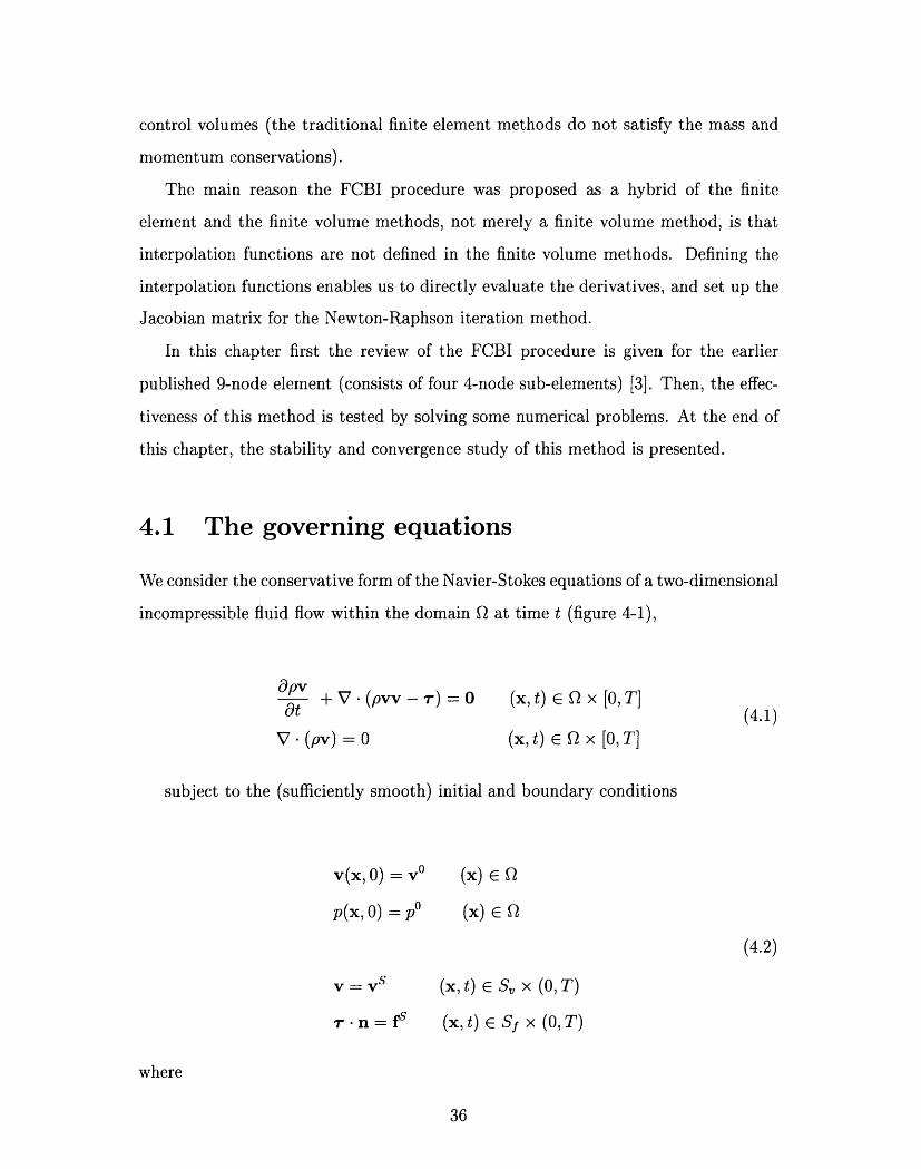
4.1 The governing equations

We consider the conservative form of the Navier-Stokes equations of a two-dimensional

incompressible fluid flow within the domain Q at time t (figure 4-1),

9PV + v. (pvv - A) = o (x, t) E Q x [O, T]19t (4.1)

V (pv)=O (x, t) E Q x [O, T]

subject to the (sufficiently smooth) initial and boundary conditions

v(x, O) = v ° (x) e Q

p(x, O) = p0 (x) Q

(4.2)

= VS (x, t) S x (0, T)

.r n = f (x, t) Sf (0, T)

where

36

r = r(v, p) = -p I + /z [Vv + (Vv)T]

In equations (4.1-4.3), /u is the viscosity, p is the density, vS are the prescribed

velocities on the boundary S,, fs are the prescribed tractions on the boundary Sf

(S = Sv U Sf, Sv n Sf = 0) and n is the unit vector normal to the boundary.

SV

Figure 4-1: The two-dimensional incompressible fluid flow problem considered

The finite element solution of the Navier-Stokes equations (4.1) is obtained by

considering a weak form of these equations. Using the Petrov-Galerkin procedure

(the test functions do not correspond to the trial functions), the weak formulation of

the problem can be given as

Find vh Ei Vh, uh E Uh and Ph E Ph such that

wh [ Ot + v (p UhVh - rh(UhPh)) dQ =0

(4.4)

qnhV (puh) dQ = 0

where Wh C Wh and qh E Qh.

Note that in these equations, the convective term (pvv) in equation (4.1) is re-

placed by (puhVh) in the weak formulation where vh C Vh and uh E Uh (two different

spaces are defined for the velocities but of course the functions in these spaces are

37

(4.3)

defined for the same nodal velocity variables). The idea of using these two different

spaces lies in that it is the convective term that for high Reynolds numbers introduces

the instability and oscillation in the numerical solution . Hence, the convective term

needs to be interpolated exponentially. Therefore, we replace the convective term

(p VhVh) by (p UhVh) and we define the interpolation functions to be exponential in

Vh and linear in Uh. Another reason is that then the FCBI scheme is also applicable

to any other transport equation, for example, the advection-diffusion equation where,

in the convective term, the temperature would be interpolated in Vh and the velocity

in Uh.

4.2 The fluid flow discretization

The spaces used in the finite element procedure depend on the elements chosen to

discretize the volume Q. In this chapter, we consider the earlier published 9-node

element (consists of four 4-node sub-elements) [3].

A mesh of elements is shown in its natural coordinate systems in figure 4-2. Each

9-node element is defined in the r - s coordinates with 0 < r, s < 1.0 and consists of

four 4-node sub-elements. Each sub-element is defined by four nodes of the 9-node

element and is used for the interpolation of velocities. The pressure is interpolated by

the four corner points in each element. Hence, for the definition of the spaces Vh, Uh

and Ph, we refer to the sub-elements and elements respectively. The sub-element is

defined in -- 77 coordinates with 0 < , rl < 1.0. To obtain the matrices or derivatives

in x - y coordinates, the usual isoparametric transformation is used [1].

The trial functions in Uh are defined in each sub-element as,

or h4 ] [ (45)or

38

4

(a) 9-node elements

A

A X3

C

h1A

Ax2

L

e

b

a..........

Ax'(b) sub-element

A X4

d

2

Figure 4-2: 9-node elements and a sub-element in isoparametric coordinates

39

I M�� - ( I

I P.wqp MMMWM

1

l

(4.6)h = l

hu = (1 - O)7

with 0 < , , < 1.

Similarly, the trial functions in the space Ph are given in each element as,

hP

hp r[1-s (4.7)

or

h = (1 - r)(1- s)

h = r(1 - s)

h = rs

h = (1 - r)s

(4.8)

with < r, s < 1.

The trial functions in Vh are defined using the flow conditions along each side of

the sub-element. The functions are, for the flux through ab (Fig. 4-2),

[h

- h2v 4h3hv3

1-X1 1-X2x -l 1-x2X1 2 l[

1- A

77[ 1-77 (4.9)77]

40

or

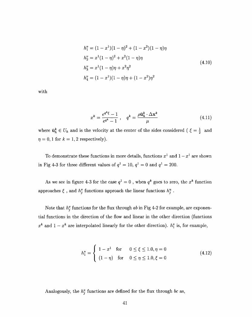
hV = (1- - 1)2 + (1 - X2 )(1 - 1)77

hV = x1(l - 1)2 + 2(1 - )1

h = Xl ( - 1) + 212

hV = (1 - xl)(1 - 71)7 + (1 - x2)12

k qk q = Pfili Axk

e q k -1 ' I =

(4.10)

(4.11)

ilh E Uh and is the velocity at the center of the sides considered ( = 1 and

1 for k = 1, 2 respectively).

demonstrate these functions in more details, functions x1 and 1 -x 1 are shown

4-3 for three different values of ql = 10, ql = 0 and ql = 200.

As we see in figure 4-3 for the case ql = 0 , when qk goes to zero, the xk function

approaches ' (, and h functions approach the linear functions hj .

Note that h functions for the flux through ab in Fig 4-2 for example, are exponen-

tial functions in the direction of the flow and linear in the other direction (functions

xk and 1 - xk are interpolated linearly for the other direction). h is, for example,

h= {I

1 -x 1 for

(1-71) for

0 < < 1.0,7 = 0

0 < < 1.0o, = 0

Analogously, the h functions are defined for the flux through bc as,

41

with

where

7 = 0,

To

in Fig

(4.12)

ql = 10

q=O0

q'= 200

1 -x'

.......... X1

.... 1 l-x'.......... X I

1-x'

.......... X1

Figure 4-3: The demonstration of x1

the three different values of ql = 10,and 1 - x1 functions for the flux through ab forql = 0 and ql = 200

42

.········· ·· ·· · ·· ··

h = (1 - 3)(1 - )2 + (1 _ x4)(1 - ')

hV = (1 - x3)(1 -_ ) + (1 - 4) 2 (4.13)

hn = X3(1 - )¢ + X462

h4 = x3(1 _ )2 + x4(1 - )

with

k eq - k PUi' A xk (4.14)a: qk q (4.14)e

q k-1 I I

where Uh e Uh and is the velocity at the center of the sides considered ( = 2and

= 0, 1 for k = 3, 4 respectively).

Note that the trial functions h, satisfy the requirement E h = 1.

The elements in the space Qh are step functions. Referring to Fig. 4-2(a), we

have, at node 2, for example,

1 for (r,s) E [ 1] [0, (4.15)hq = '~"I C L2 2(4.15)

0 elsewhere

Similarly, the weight functions in the space Wh are also step functions. Considering

the sub-element shown in Fig. 4-2(b), at node 1, for example,

1 for (, ,r7) [0, ] [, (4.16)

0 elsewhere

Then, the velocities Uh, vh (in each sub-element) and the pressure Ph (in each

element) , interpolated with the trial functions in Uh, Vh and Ph respectively, are

43

4

h = E hu Vhii=1l

4

Vh= h Vhi (4.17)i=l4

Ph = Sh Phii=l

where Vhi and Phi are the nodal velocity and pressure variables.

We again mention that although two different spaces are defined for the velocities

but of course h and hy functions are defined for the same nodal velocity variables Vhi.

The idea of using these two different spaces lies in that it is the convective term that

for high Reynolds numbers introduces the instability and oscillation in the numerical

solution. Hence, the convective term needs to be interpolated exponentially. We

replace the convective term (p VhVh) by (p UhVh) and we define the interpolation

functions to be exponential in Vh and linear in Uh. Another reason is that then the

FCBI scheme is also applicable to any other transport equation, for example, the

advection-diffusion equation where, in the convective term, the temperature would

be interpolated in Vh and the velocity in Uh.

Considering the steady-state condition, equation (4.4) is then,

jwhV [p Uhh -- h(Uh,Ph)] dQ = 0(4.18)

qhV (p uh) dQ = 0

Assembling equations 4.18 for all the control volumes in the body, and using the

divergence theorem to take these integrals around the control volumes we get

44

SA wh n. [p UhVh - rh(Uh,Ph)] dS = 0(4.19)

s jqh n (p Uh) dS = O

where the momentum and the continuity equations are summed over the control

volumes of the velocity points and pressure points respectively, S is the surface of

each control volume (that corresponds to the length in two-dimensional problems), n

is the unit normal vector pointing to the outside of the control volume and

'h = -Ph I + p [Vuh + (Vuh)T] (4.20)

The flux is then calculated with the interpolated values at the center of the sides

of the control volumes. For example, the flux through ab (Fig. 4-2) is obtained as

bn f dS = n. f()l=1/2, 77=1/4 Sab (4.21)

where ASab :is the length of ab and

f() = p UhVh + Ph I - [Vuh + (Vuh)T] (4.22)

in the momentum equation and

f(~) = p Uh (4.23)

in the continuity equation.

Replacing Uh, vh and Ph from the equations (4.17) , when Wh and qh are the unit

step functions (for the control volumes of the velocity and pressure points respec-

tively), the corresponding linearized finite element matrix equations are,

45

KVV

KVyVy

Kpvy

AVx

Avy

Ap

f Rv1 Fv

- Fv

0 FP Fp(4.24)

Kvzp

KvYp

0

where Ave, Avy, Ap, are the increments of the velocity in x

y direction and pressure with respect to the last iteration; Rv~

cretized load vectors and Fvx, Fv,, Fp contain terms from the

Using the full Newton-Raphson iteration method, for a mesh

ments, we get

direction, velocity in

and Rv are the dis-

linearization process.

of non-distorted ele-

nx ay x (qi hv - h)19 d a Yz~KV.VX(j i) = E Whj J

Oy3Ci

Oxax hi- + E Whji J

ny e Oay (Q ih i - h ui)19~1 dZ'

OyWhj ,u nsx -

Orl

Kv vl/ (ji) = -Ei

9 [a(gmh-h hu)OaX aO(vhi)x

Whj IL ny a aOx h u

5d ax i

(Vhm)x]

(4.25)

ax O19 O(g9mh - h)Whj nfly Oy [ ((Vhm)x]

Y ~ 1 Y a(hi), +E

J

Kvp (j,i) = Ei

yWj nwhj nlx hi

46

+EJ.

j,i) = -E

DyWhj / nPx O

K " j )=.

y Drlwhj / n ar aO hi '

2 I (9mh-h h)

x D (Vhi)x (Vhm)y]

whj nZ ay a (qihv - hiu)

(4.26)

dx drWhj I ny a, ay hi + S Whij

Ox arny aJ ay

dx DrlWhj ny a ay

JixWhj

ny a h droxfu i

In these equations, f = 2 f 72 f d or f - 2 fe2 f d based on the direction of

the flux, the velocities are the values calculated at the end of the previous iteration;

(vhm)x = (Vhm)/-1, (Vhm)y = (hm)7 - 1 where the repeated subscript m denotes sum-

47

-Ej(qihv- h,)z %I/ rl

+EJ

a(gmhv - hu)I l- _ (Vhm)y]

Kvp(j, i) =

Kpv (j, i) = E qhj nxi

y J s19s % dKPVY (j, i) = 5: qhj

J

(4.27)

Kvyv (.

mation, the subscripts x and y show the direction of the velocity and the subscript

I stands for the iteration number . The terms used in these equations are as follows

(for the control volumes which have no sides on the boundary),

For l = 0, 2 = (flux through ab )· For 7~1--' 0, ? 2

1

1K un=

-33

[

-1

_J

-1 1

-1 1

(4.28)Sih - h = D h(r1)hT(77)

h(r)hT () =7 2

2 1

'0 5

hi 2 h dnfO

where

(4.29)B2

_A 2

and

{

eAk _ qk

Bk = Ak + qk(4.30)

* For r , r2 = 1

48

BiD = A

1hi = -

1

h" 2

[

[

gih - h =

-1 -3

1 3

-1

-1 i

hi 2 hi 0.5where D is as equation 4.29.

where D is as equation 4.29.

* For , = 0, 2 = (flux through bc )· F~r~l-:0,~~2

49

D h(n)hT() (4.31)

hi=1 -3 3]4 -1 I

i- - [2 1 1

gih - h = h(6)hT (6) E

h- 2j h~0.5hp = 2 hP d<

where

-A 1

_A 2 (4.33)

and

{

Ak = q

Bk = Ak + qk

* For I -= ,6 = 1

50

(4.32)

(4.34)

BiE = :

1

1

- 2

-1 1

-3 3

-1 -1

1

gih v - hi = h(S)hT (~) E(4.35)

1

0.5

where E is as equation 4.33.

After the system of equations (4.24) is solved, the velocity and the pressure incre-

ments are obtained. The velocities and pressures are then updated as,

(Vh) = AVx + (Vh)x- 1

(4.36)(Vh)/ - AVy + (Vh)y 1

(ph)' = Ap + (h)'- 1

4.3 Fundamental properties of the FCBI proce-

dure

* Using two different spaces Uh and Vh for the velocities

In the FC1BI procedure, the convective term (p vv) in equation (4.1) is replaced

51

h (~)hT (S) = I [ 2

by (p uhvh) in the weak formulation where vh E Vh and uh E Uh (two different spaces

are defined for the velocities but of course the functions in these spaces are defined

for the same nodal velocity variables). The idea of using these two different spaces

lies in that for high Reynolds numbers it is the convective term which introduces the

instability and oscillation in the numerical solution. Hence, the convective term needs

to be interpolated exponentially. Therefore, we replace the convective term (p VhVh)

by (p UhVh) and we define the interpolation functions to be exponential in Vh and

linear in Uh. Another reason is that then the FCBI scheme is also applicable to any

other transport equation, for example, the advection- diffusion equation where, in the

convective term, the temperature would be interpolated in Vh and the velocity in Uh.

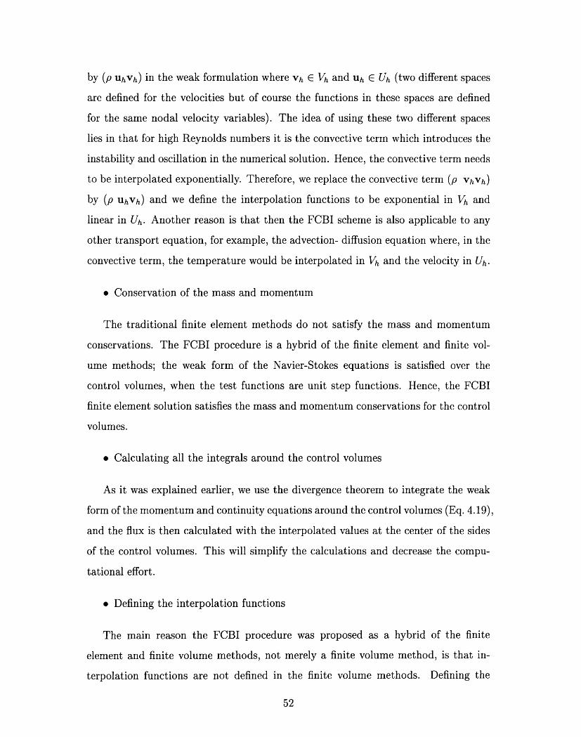
* Conservation of the mass and momentum

The traditional finite element methods do not satisfy the mass and momentum

conservations. The FCBI procedure is a hybrid of the finite element and finite vol-

ume methods; the weak form of the Navier-Stokes equations is satisfied over the

control volumes, when the test functions are unit step functions. Hence, the FCBI

finite element solution satisfies the mass and momentum conservations for the control

volumes.

* Calculating all the integrals around the control volumes

As it was explained earlier, we use the divergence theorem to integrate the weak

form of the momentum and continuity equations around the control volumes (Eq. 4.19),

and the flux is then calculated with the interpolated values at the center of the sides

of the control volumes. This will simplify the calculations and decrease the compu-

tational effort.

* Defining the interpolation functions

The main reason the FCBI procedure was proposed as a hybrid of the finite

element and finite volume methods, not merely a finite volume method, is that in-

terpolation functions are not defined in the finite volume methods. Defining the

52

interpolation functions enables us to directly evaluate the derivatives, and set up the

Jacobian matrix for the Newton-Raphson iteration method.

4.4 Numerical examples

To study the effectiveness of the FCBI procedure, we consider the driven cavity flow

problem and the S-channel flow problem in this section. The results presented are

obtained using the FCBI 9-node elements.

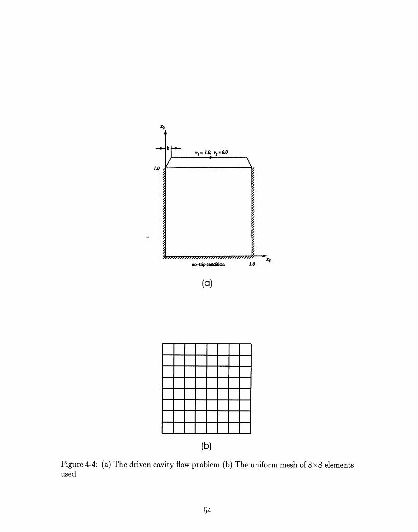
4.4.1 The driven cavity flow problem

The cavity flow problem shown in figure 4-4(a) has occupied attention of the scien-

tific computational community since the pioneering paper of Burggraf back in 1966

[8]. In early papers finite difference methods and finite volume methods were used

to overcome the difficulty of solving this problem for high Reynolds number flows

and to improve the accuracy of the solution. For example, Gatski et al. used a

velocity-vorticity formulation [13] and Ghia et al. used a finite difference method

in conjunction with a multigrid procedure [11]. However, the new velocity-vorticity

finite volume methods [9], [23] are more stable (up to Re=10,000) than the previous

finite difference or finite volume methods but still less stable than some of the upwind

finite element methods.

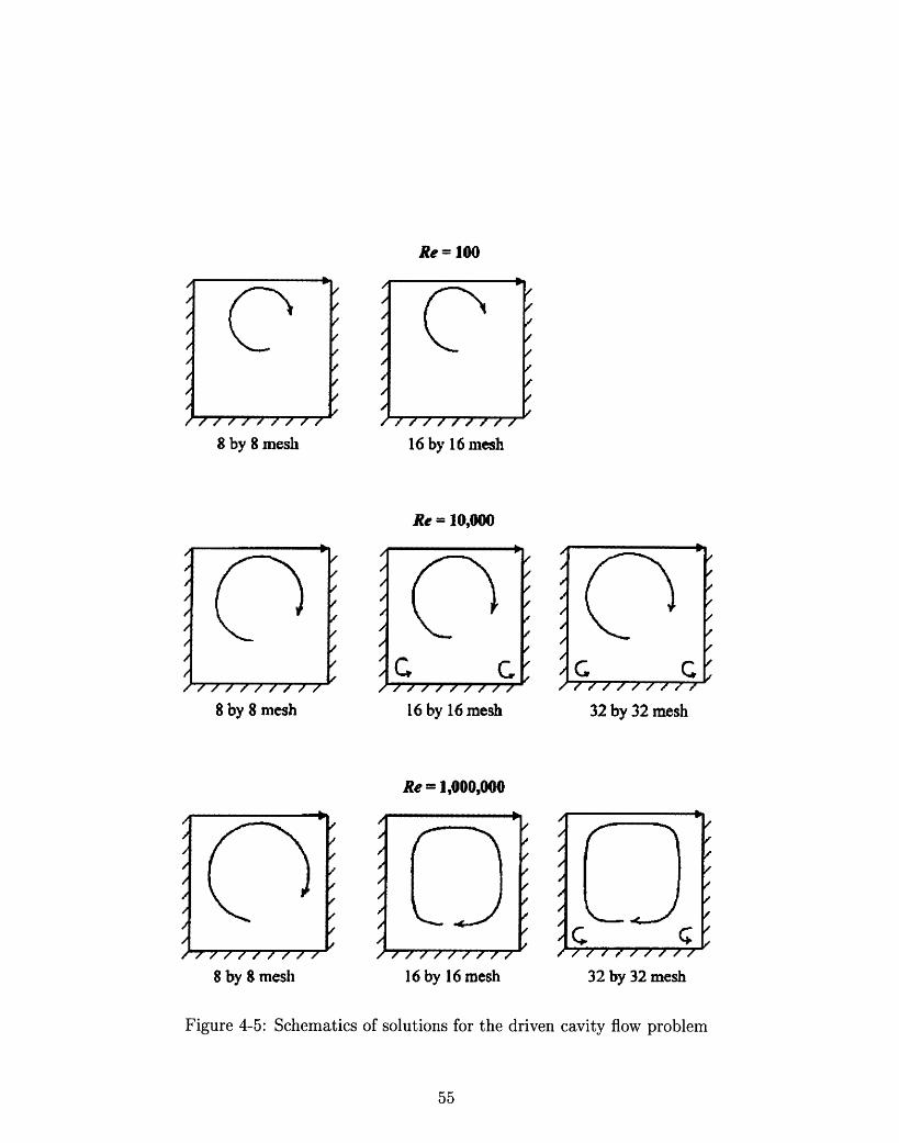
If the uniform mesh of 8x8 elements shown in Fig. 4-4(b) is used (this is a coarse

mesh), reasonable results are obtained. Of course when the mesh is refined, more

details in the flow could be captured as it is illustrated in figure 4-5. When the

Reynolds number is high, there are circulations near the corners, also the flow solution

hardly changes from a certain Reynolds number onwards.

The driven cavity flow problem for the uniform mesh of 8x8 elements shown in

Fig. 4-4(b) is solved for different Reynolds numbers 1, 100, 10,000 and 1,000,000. The

velocity and the pressure solutions are shown in Fig. 4-6 and Fig. 4-7 respectively.

Furthermore, in Fig. 4-8 vorticity is plotted for different Re numbers.

To study the effectiveness of the FCBI procedure, the horizontal velocity at the

53

1.0F v, 1.0. Duo

1.0nooslip cron

(a)

XI

(b)

Figure 4-4: (a) The driven cavity flow problem (b) The uniform mesh of 8x8 elementsused

54

---

--- VVV>2z~ -- 7-7 - wpo2 7- 71.1-"77 -

\I....-

Re = 100

· by 8 mesh f

8 by 8 mesh

//.I0/1!1

I

A.

I

A.

A.

A.

A., f e f e f .

16 by 16 mesh

Of - I~~~'

IC c

8 by 8 mesh 16 by 16 mesh 32 by 32 mesh

Re = 1,000,000

8 by 8 mesh 16by 16 mesh 32 by 32 mesh

Figure 4-5: Schematics of solutions for the driven cavity flow problem

55

.j

I0

I1

I1

I0

A'

0,

A,1

/1

0,

A,

A.

A.0.

A.

Re- 10,000

/A --

I

A'

'.

.l

00,

00,/.

A,

A,

A,

A./1

I

//,/////// A.

.e

IA.'

I"IA.

0,'lo/

Oe

/C ------ C

A.

A.

0.

A.

A.

I -14 IR

I 7 "I l

A0,

A0,

A,

A.

A,

A'0

A'

0'

A'

A'

A'

A,1

A'0/

0,

A''I

A,

00.

p1

A /I

It( IICI

00,

A.

ol

/,!0,A'/./.

I- - - - - - - - - I

0 P I000

00

0

0

00

0

11 - - - -I I I - -

01 P0

0

0

0

I

II

11, ---

I

0

0

1

I

I

I

I0000

0f

I

I

o

I

0

1

.1

0

Re= I

Figure 4-6: The velocity solutions of the driven cavity flow problem for Re = 1, 100,10,000, 1,000,000 for the uniform mesh 8 x 8 elements

56

/I I I ~~I I

I I ~ ~ I I

I I / / /

I j

'1/I

,/ /

Re = 1,000,000Re = 10,000

I 1~~~~~~~~~~~ /I/ I

Il I

/ I

/, ......

I I . III / - - I / I

8 t # t S o - - - - - / I I

// lf t ,, l .....

s \ \ / / /

l \ \ i s r , ,/ \ > - - - ' ' I LL/ / v v v - - ' ' ' 1 11- z

iC·r�U:

-- - -- - -- - - -- ·

-- - -- -

- -- - - - -- - - - - -- - --

1-rsu; -

.P d.--

-- - -- -- - -- -

- - - -

Re= 100

Re =10,000PRESSURE

19.056417.4846I 15.9127

-14.3409-: 12.7891

11.19729.625418.053586.481754.909913.338081.766250.194413-1.37742-2.94925

I

0.

0.E

0.70.E

<0.E

0.4

0.3

0.2

0.1

Re =1

PRESSURE129.015110.86292.709474.5568

, 56.404238.251620.0991.94636

-16.2063-34.3589-52.5115-70.6641-88,8167-106.969-125.122

Re = 100

PRESSURE3.53543.272993.010582.74817

i tl2.485752.223341.960931.698521.436111.173690.9112820.648870.3864580.124046

-0.138366

0.5X

e = 1,000,000PRESSURE

1803.281646.841490.41333.96

1177.531021.09864.651708.214551.776395.339238.90282.4642-73.9733-230.411-386.848

xX

Figure 4-7: The pressure solutions of the driven cavity flow problem for Re = 1, 100,10,000, 1,000,000 for the uniform mesh 8 x 8 elements

57

O.C

0.E

0.7

O.E

0.4

0.3

0.2

0.1

0.

0

0

0

0

0

0

0

0

0

v.vX

0.S

0.

0.

0.6

0.1

0.,

O.'

0.10

*rlLI1I I roln�nul

--- ----~~~~~~~ I I�L

I

Re=- 00

Figure 4-8: Contours of the vorticity for different Re numbers for uniform mesh 8x8 elements. The contour levels shown for each plot are -5.0, -4.0, -3.0, -2.0, -1.0, 0.0,1.0, 2.0, 3.0, 4.0 and 5.0

58

Re=1000 Re=5000

*I1 .-W

Re=400

T�oll·cnui - ---s

_

vertical centerline, and the vertical velocity at the horizontal centerline are plotted

and compared with the solutions of the Ghia et al. [11] in figure 4-9 and 4-10

respectively. In these figures, the solution obtained by Ghia et al. is shown by "+",

this solution is assumed to be the exact solution.

As it is clear from figures 4-9 and 4-10, the FCBI scheme yields reasonable

solutions for the driven cavity flow problem (these results are obtained for the coarse

mesh of 8x 8 elements). In order to improve the accuracy of the solution, the mesh

needs to be refined. Also, close to the boundaries, a finer mesh is required in order

to have higher spatial accuracy (a non-uniform mesh).

Note that the FCBI solution obtained for the coarse mesh of 8x 8 elements (16x

16 sub-elements) is stable up to Re=1,000,000 although no upwind parameter is used.

Hence, defining two different spaces for the velocities and defining the trial functions

in the space Vh to be exponential functions, as it is done in the FCBI procedure,

stabilizes the solution even for very high Reynolds numbers.

4.4.2 The S-channel flow problem

The second problem considered in this chapter, is the S-channel flow problem shown

in Fig. 4-11 (a). This problem is hard to solve for high Reynolds numbers. If the

mesh shown in Fig. 4-11(b) is used (this is a coarse mesh), reasonable results are

obtained. Of course when the mesh is refined, more details in the flow could be

captured as it is illustrated in figure 4-12. When the Reynolds number is high, there

are circulations near the corners, also the flow solution hardly changes from a certain

Reynolds number onwards.

The S-channel flow problem for the mesh shown in Fig. 4-11(b) is solved for

different Reynolds numbers 1, 100 and 10,000. The velocity and the pressure solutions

are presented in Fig. 4-13 and Fig. 4-14 respectively.

Note that the FCBI solution obtained for the coarse mesh used, is stable up to

Re = 10,000 although no upwind parameter is used. Similar to the cavity flow

problem, defining two different spaces Vh and Uh for the velocities and defining the

trial functions in the space Vh to be exponential functions, as it is done in the FCBI

59

co

C

Re=100

Re=1000 Re=5000

Figure 4-9: 'rhe horizontal velocity at the vertical centerline of the cavity for Re =100, 400, 1000, 5000 when the uniform mesh 8 x 8 elements is used

60

Re=400

.

Re=100

Re=1000 Re=5000

Figure 4-10: The vertical velocity at the horizontal centerline of the cavity for Re =100, 400, 1000, 5000 when the uniform mesh 8x 8 elements is used

61

Re=400,,

Xl

(a)

I I I L IAF I I I I I I I

i i i I_

(b)

Figure 4-11: (a) The S-channel flow problem (b) The mesh used

62

lI I LI - - - - .I i .· · · ir·l...lii -r i I J·~ i l l l l

- I I

I I r I h E

__ _ _�� ___ _� �.� .. � - I

- -- · · --· r--i

I i i i i, i I iI I I I I I I I

I iB E

1

coarser mesh

L(a)

coarser mesh finer mesh

ii

I

'^ " - - . ...- - .V

I "/j

(b)

Figure 4-12: Schematics of solutions for the S-channel flow problem (a) Re = 100,(b) Re = 10,000

63

finer mesh

I

4I9

I

iI

9,. .... w s .

... . ...

,_ ., ... _ ._ _ . . _ I

i!.. .. . .- - - ., 7 ,1

i

i

I

I

I

I

I

i

I

I

i

'. .. ... .. . " -i

I

II

I

J

procedure, stabilizes the solution for high Reynolds numbers.

For further evaluation, nodal pressures along the lower boundary and upper

boundary of the S-channel are shown in figure 4-15. These solutions are obtained

using the mesh shown in Fig. 4-11(b) and two times finer and coarser meshes when

Re = 100. The nodal pressures obtained from ADINA program (the FCBI procedure

for 4-node elements) are given in figure 4-16. These pressures are the same as the

pressure solutions in Fig. 4-15.

4.5 Further study of the FCBI scheme

4.5.1 Stability of the FCBI scheme

In the FCBI procedure, the convective term (p vv) in equation (4.1) is replaced by

(p UhVh) in the weak formulation where vh E Vh and uh E Uh (two different spaces are

defined for the velocities but of course the functions in these spaces are defined for the

same nodal velocity variables). In addition, the trial functions in Vh are exponential

functions which are evaluated based on the direction of the flux (the trial functions in

Uh are linear functions). The idea of using these two different spaces lies in that it is

the convective term which introduces the instability and oscillation in the numerical

solution when the Reynolds number is high. Hence, the convective term needs to be

interpolated exponentially.

Although no upwind parameter is used to make the FCBI procedure stable, defin-

ing two different spaces for the velocities, exponentially interpolating functions in

the Vh space and evaluating the pressure interpolation functions such as the inf-sup

condition is satisfied, stabilizes the FCBI procedure in a natural way.

In this section, the driven cavity flow and the S-channel flow problems are once

again considered to compare the stability of the FCBI procedure to some of the

upwind techniques in [14].

Table 4.1 compares the stability of the FCBI procedure to the stability of the

streamline upwind/Petrov-Galerkin (SUPG) method and the Galerkin/least-squares

64

Re=

Re = 100

Re = 10,000

Figure 4-13: The velocity solutions of the S-channel flow problem for Re =1,100, 10, 000 for the mesh shown in figure 4-11 (b)

65

PRESSURE205.978192.006178.033164.061

PRESSURE39548.336888.734229. 11 ...

Figure 4-14:

Re = 1.0

RelO00

The pressure solutions of the S-channel flow problem for Re =1,100, 10, 000 for the mesh shown in figure 4-11 (b)

66

4.5

4

3.5

0.13-, 2

1.5 -

05to

0 1 2 3 4 5 6 7 8 9 10

Distance along lower boundary

4.5 . ,

3.5 ......

3 . a

2.5

2o A The coarse mesh

1.5* The mesh shown in Fig. 4-11 (b)

The fine mesh *.0.5

0 1 2 3 4 5 6 7 8 9

Distance along the upper boundary

Figure 4-15: Pressure solutions obtained by the FCBI procedure using the meshshown in Fig. 4-11(b) and the two times finer and coarser meshes when Re = 100

67

4 a.

':. .. . .-::::)~~~~~~~***·*~*,*****~ · e~ m s

4 a

*+ I

A The coarse mesh . ,4 "

I The mesh shown in Fig. 4-11(b) ....itl

* The fine mesh

.", , , , , , .l~~~~~~~~&

c

. . . . . .

0 1 2 3 4 5 6 7 8 9Distance along lower boundary

.I++++

1 2 3 4 5 6Distance along upper boundary

7 8 9

Figure 4-16:shown in Fig.

Pressure solutions obtained by the ADINA program using the mesh4-11(b) and the two times finer mesh when Re = 100

68

4.5

4

3.5

0o

u)

C.

0Z

3

2.5

2

1.5

I--t + + + + + +++-I-+ +)0000000000000000+

0 +00 + + +

000000

+ forthe mesh in Fig.4-11(b)o for fine mesh

00

0oP

0

O ., , , , * , , ,~~~

0.5

0

4

4

3.5

O

/)2a)3.

z

3

2.5

2

1.5

+ ++OOOOO OOo

0 0

o+ forthe mesh in Fig.4-11(b) Io for the fine mesh o

00

o0o0d 00

0

1

0.5

0

0

I I I I I I [

'J

1

I

,.,-I -·

(GLS) method. In this table, a uniform mesh of 20x20 elements is used (20x20

sub-elements in the FCBI procedure). The number of iterations required to solve the

problem, is also shown for the ADINA program (FCBI 4-node elements).

The S-channel flow problem shown in Fig. 4-11(a) is used as our second example.

In Table 4.2, the number of iterations required to solve the problem, are given for the

upwind/Petrov-Galerkin (SUPG) method, the Galerkin/least-squares (GLS) method,

the FCBI scheme for 9-node elements (each element consists of four 4-node sub-

elements) and the ADINA program (FCBI scheme for 4-node elements). In this

Table, a mesh of 480 elements is used (120 elements and 480 sub-elements in the

FCBI procedure).

To obtain results given in these tables, Newton-Raphson iteration method is used

and (*) denotes iteration not converged within the allowable 35 number of iterations.

In these tables the convergence tolerance is 10-6 for the normalized norms Rv I vhI- IIPhl

and Rp = l/xPh1

As it is clear in both the driven cavity problem and the S-channel flow problem,

the FCBI 9-node and 4-node elements (ADINA) give more stable solutions than the

SUPG and GLS methods. The FCBI 4-node elements yield more stable solutions

than the 9-node elements but as we see later on in this chapter, the 9-node element is

more effective in capturing flow details, velocity and vorticity fields and showing the

circulations for high Reynolds numbers. The S-channel flow problem is more sensitive

for higher Reynolds numbers since there will be circulations near the corners.

4.5.2 Accuracy of the FCBI scheme

In this section the L2 and H1 norms of the velocities and the L2 norm of the pressure

are used to measure the errors in the FCBI method. Of course to study the accuracy

and convergence of the FCBI 9-node element, more appropriate posteriori error es-

timator could be found. The L2 and H1 norms of the velocities and L2 norm of the

pressure considered here are as,

69

Re SUPG GLS FCBI ADINA

4001000200040008000

10000120001500018000200002400026000280003000040000450004800050000

1000001,000,000

88

7

88

6444444445

88991010

10

11

11

11

11

1112121216

7889101010

1011

11

11

11

11

12121212

1213

15

Table 4.1: Number of iterations required to solve the driven cavity flow problem fordifferent Re numbers.

70

Re SUPG GLS FCBI ADINA

Re SUPG GLS FCBI ADINA

250500750

100015002000400070008000

1000015000200004000050000

8*

5

6671011

1216*

78999911

12121314

1516*

Table 4.2: Number of iterations required to solve the S-channel flow problem fordifferent Re numbers.

U - Uh IL2

I| U-Uh 1:; =

eover sub-elements

over sub-elements

(u - Uh)2 dxdy +

IJ(u - h)2 dxdy +

over sub-elements

oover sub-elements

J(U - Uh)2 dxdy

(4.37)

f(u - Uh)2 dxdy

+ Eover sub-elements

(u - uh), x dxdy +

+ e J(u-uh)xdxdy +over sub-elements

oover sub-elements

oover sub-elements

II/J

(u - Uh)2, dxdy

(u - Uh), , dxdy

(4.38)

71

SUPG GLS FCBIRe ADINA

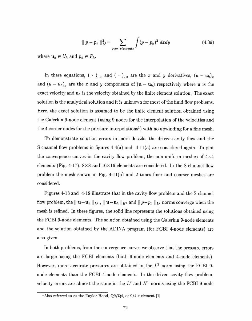
P - Ph IIL2= E f(P h) dxdy (4.39)over elements

where Uh E Uh and Ph E Ph.

In these equations, ( ), and ( ),y are the x and y derivatives, (u - Uh)x

and (u - Uh)y are the x and y components of (u - Uh) respectively where u is the

exact velocity and uh is the velocity obtained by the finite element solution. The exact

solution is the analytical solution and it is unknown for most of the fluid flow problems.

Here, the exact solution is assumed to be the finite element solution obtained using

the Galerkin 9-node element (using 9 nodes for the interpolation of the velocities and

the 4 corner nodes for the pressure interpolations l) with no upwinding for a fine mesh.

To demonstrate solution errors in more details, the driven-cavity flow and the

S-channel flow problems in figures 4-4(a) and 4-11(a) are considered again. To plot

the convergence curves in the cavity flow problem, the non-uniform meshes of 4x4

elements (Fig. 4-17), 8x8 and 16x16 elements are considered. In the S-channel flow

problem the mesh shown in Fig. 4-11(b) and 2 times finer and coarser meshes are

considered.

Figures 4-18 and 4-19 illustrate that in the cavity flow problem and the S-channel

flow problem, the 11 U-uh L2 , 11 U-Uh H1 and P-Ph [[L2 norms converge when the

mesh is refined. In these figures, the solid line represents the solutions obtained using

the FCBI 9-node elements. The solution obtained using the Galerkin 9-node elements

and the solution obtained by the ADINA program (for FCBI 4-node elements) are

also given.

In both problems, from the convergence curves we observe that the pressure errors

are larger using the FCBI elements (both 9-node elements and 4-node elements).

However, more accurate pressures are obtained in the L2 norm using the FCBI 9-

node elements than the FCBI 4-node elements. In the driven cavity flow problem,

velocity errors are almost the same in the L2 and H1 norms using the FCBI 9-node

1Also referred to as the Taylor-Hood, Q9/Q4, or 9/4-c element [1]

72

Figure 4-17: The non-uniform mesh of 4x4 9-node elements used

elements and the FCBI 4-node elements. Note that the solution using the Galerkin

9-node elements is not stable for the coarsest mesh and is not included in figure 4-18.

In the S-channel flow problem, velocities are better predicted using the FCBI 9-node

elements than the FCBI 4-node elements in both L2 and H1 norms. The solution

obtained by the ADINA program (using FCBI 4-node elements) for the coarsest mesh

is not accurate enough and therefore not included in figure 4-19.

Since in the FCBI procedure two different spaces Vh and Uh are used to define

the velocities, and the trial functions in Vh are exponential functions, the rate of the

convergence of the H1 and L2 norms (the slope of the given lines in figures 4-18 and

4-19 corresponding to the FCBI 9-node and 4-node elements) is less than the rate

of the convergence using the Galerkin 9-node elements. In other words, although

defining the trial functions in Vh as exponential functions makes the solution to be

too stable (too much upwinding), it decreases the rate of the convergence of the H1

and L2 norms.

* Concluding remarks on the numerical results

Of course we can only draw partial conclusions from these preliminary numerical

results since, in particular, other fluid problems need to be considered for compre-

73

.... ... ... ... _..........

// FCBI9-node element

/ ADINA (FCBI 4-node element)

/ g

/U

-1.3 -1.1 -0.9 -0.7 -0.5 -0.3 -0.1

log (h)

Fig 4.18 (a)

-1.3 -1.1 -0.9 -0.7

log (h)

Fig 4.18 (b)

-0.5 -0.3 -0.1 0.1

74

-0.5

-1

-1.5 -

-2 -

-2.5

-3 -

-3.5 -

-4-1.5

0

-0.5

-1

-1.5

-2

-2.5

-3-11 .5

I I · I

.

-o alrkn -~~~~~/ ~Galerkin 9-n,

aode element --

FCBI 9-node element

ADINA (FCBI 4-node element) ...... -

-1.5 -1.3 -1.1 -0.9 -0.7

log (h)

Fig 4.18 (c)

-0.5 -0.3 -0.1 0.1

Galerkin 9-node element

FCBI 9-node element

ADINA (FCBI 4-node element) ..........

/I

-1.3 -1.1 -0.9 -0.7

log (h)

Fig 4.18 (d)

-0.5 -0.3 -0.1 0.1

Figure 4-18: Comparison of the FCBI 9-node elements, FCBI 4-node elements andthe Galerkin 9-node elements for the driven cavity flow problem (Re=1000). Inthis figure, the x coordinate represents log h when h is the element size and the ycoordinate for each case is a) log lu-UhlL2 , b) log lu-hlH1 ,c) log IIv-PhIL2 , d)

Ilull2 +Iuuh H pl

log ( IulH1 + P-pL2 )11U1H1 HIIvIL2

75

0

-1

-2

-3

-4

-5

U

-0.5

-1

-1.5

-2

-2.5

-3-1.5

n_....

it) ........... r1

-1 .5 -1 -0.5 0

log (h)

Fig 4.19 (a)

76

0

-0.5

-1

-1.5

-2

-0.5

-1

-1.5-1 .5 -1 -0.5 0

log (h)

Fig 4.19 (b)

-A

U-

ir

Galerkin 9-node element ----

FCBI 9-node element

ADINA (FCBI 4-node element) ..............

-1 -0.5

log (h)

Fig 4.19 (C)

-1 -0.5

0

0

log (h)

Fig 4.19 (d)

Figure 4-19: Comparison of the FCBI 9-node elements, FCBI 4-node elements and theGalerkin 9-node elements for the S-channel flow problem (Re=100). In this figure, thex coordinate represents log h when h is the element size and the y coordinate for each

case is a) log l1u-UhL2 b) log 11u-uhll , c) log IP-Ph L2 d) log (Iu-UhIH + 1P-PnhIL2IlullL2 '1IH1 IullL Ilull2 - H it 2 )'

77

0

-0.5

-1

-1.5

-2

-2.5

-3-1.5

n_

-0.5

-1

-1.5-1.5

hensiveness.

From these numerical results, the FCBI 9-node element (consists of four 4-node

sub-elements) appears to be stable for high Reynolds numbers although no upwind

parameter is used, and predict the solution reasonably accurate.

Of course, in order for the solution errors to be small, the mesh needs to be refined.

However, the convergence curves display a small rate of convergence when the FCBI

9-node element is used.

78

Chapter 5

A new FCBI 9-node element

The analysis of fluid flows with structural interactions has captured much attention

during the recent years. Such analysis is performed considering the solution of the

Navier-Stokes fluid flows fully coupled to the non-linear structural response. However,

a fully coupled fluid flow structural interaction analysis can be computationally very

expensive. The cost of the solution is, roughly, proportional to the number of nodes

or grid points used to discretize the fluid and the structure [1].

In order for interaction effects to be significant, the structure is usually thin and

can be represented as a shell, hence not too many grid points are required. The large

number of grid points and consequently number of equations in fluid flow structural

interaction problems (FSI) is due to the representation of the fluid domain. For high

Reynolds number fluid flows, to have a stable solution, more grid points are required.

In order to decrease the number of grid points in the fluids (using a coarser mesh) and

still have a stable solution, the flow-condition-based interpolation (FCBI) procedure

was introduced [2], [3], [4].

As it was already mentioned in chapter 4, the FCBI procedure is a hybrid of the

finite element and the finite volume methods. The test functions for both the conti-

nuity and the momentum equations are step functions and the governing equations

are written over control volumes. Hence, the mass and momentum conservations are

satisfied locally. Ideally any numerical solution for fluids should yield stable solutions

for low and high Reynolds number flows with reasonable accuracy. Of course, when

79

fine meshes are used, more details of the flow are captured and the level of accuracy

is higher. Ideally, we want our numerical scheme to yield still stable solutions with

reasonable accuracy when coarse meshes are used. In particular, this will decrease the

required number of grid points and elements in the fluid phase in the fluid-structure

interaction problems.

In order to ensure that using the coarse meshes to represent the fluid yields an

accurate enough structural response, the solution errors need to be controlled and

measured. The "goal-oriented error estimation" might be applied to assess the error in

the quantities of interest in the structure. In fluid flow structural interaction analysis,

it is ideal to use an FCBI solution scheme in rather coarse meshes together with

"goal-oriented error estimation" to control the error of the solution in the structural

response [12]. In all the FSI problems considered in [12], the flow problems are solved

using the 4-node FCBI elements available in ADINA. The error estimate then uses the

fluid flow approximation obtained with a 9-node Galerkin finite element (using the 9

nodes for the velocities and the 4 corner nodes for the pressure interpolations l ) and

the same mesh (i.e., with the same number of elements) as used with the 4-node FCBI

elements. However, Galerkin 9-node elements are unable to give stable solutions with

coarse meshes for high Reynolds number flows. Hence, it would be ideal to use 9-node

FCBI elements with much better stability and almost the same accuracy as Galerkin

9-node elements.

The earlier published 9-node FCBI elements, consisting of four 4-node sub-elements,

are illustrated and studied in chapter 4. In this chapter, it became clear that these

FCBI 9-node elements are more stable than the Galerkin 9-node elements. However,

the Galerkin 9-node elements give more accurate solutions with a higher rate of con-

vergence. Hence, in this chapter we propose a new FCBI 9-node element that obtains

more accurate solutions than the earlier proposed FCBI elements. The new 9-node

elements do not obtain the solution as accurate as the Galerkin 9-node elements but

the solution is stable for much higher Reynolds numbers (than the Galerkin 9-node

elements), and accurate enough to be used to find the structural responses.

1Also referred to as the Taylor-Hood, Q9/Q4, or 9/4-c element [1]

80

5.1 Fluid flow discretization

In chapter 4, we already introduced and studied the earlier published FCBI 9-node

element consisting of four 4-node sub-elements. In this section we present a new FCBI

9-node element.

As we already mentioned in chapter 4, in the FCBI scheme, we use a Petrov-

Galerkin variational formulation with subspaces Vh, Uh and Wh of V, and Ph and Qh

of P of the Navier-Stokes equations. The formulation used is:

Find Vh E Vh, Uh E Uh, Ph E Ph such that for all Wh E Wh and qh E Qh

wh [PUt + V (puhvh - r(uh,ph))] dQ = 0 (5.1)

jqhV (puh)dQ = 0 (5.2)

To define the spaces used in the formulation, consider Fig. 5-1, where we show the

new element in its natural coordinate system. This element is defined by nine nodes

for the interpolation of the velocities and four corner nodes to interpolate the pressure.

Let us mention that in chapter 4, each 9-node element consists of four 4-node sub-

elements and in each sub-element the four corner nodes are used to interpolate the

velocities vh and Uh. The pressure is interpolated by the four corner points in each

element. Hence, for the definition of the spaces Vh, Uh and Ph, we referred to the

sub-element and element respectively. Here, for the new 9-node element, spaces Vh,

Uh and Ph are defined for the element.

The trial functions in Uh are

81

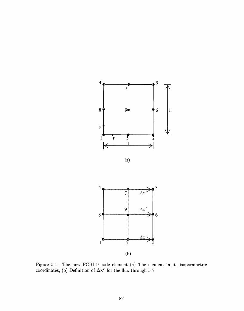
7

r 5 2

14- 1 Nj

8

S

1

/

6

\

K

1

!i

(a)

8'

1

3

1 6

(b)

Figure 5-1: The new FCBI 9-node element (a) The element in its isoparametriccoordinates, (b) Definition of Axk for the flux through 5-7

82

A \

\xI

)a*a**rararrrsaaasas*aaaer

__........ _ ,,,,, s As,,

4 3

I1

1/

7

9

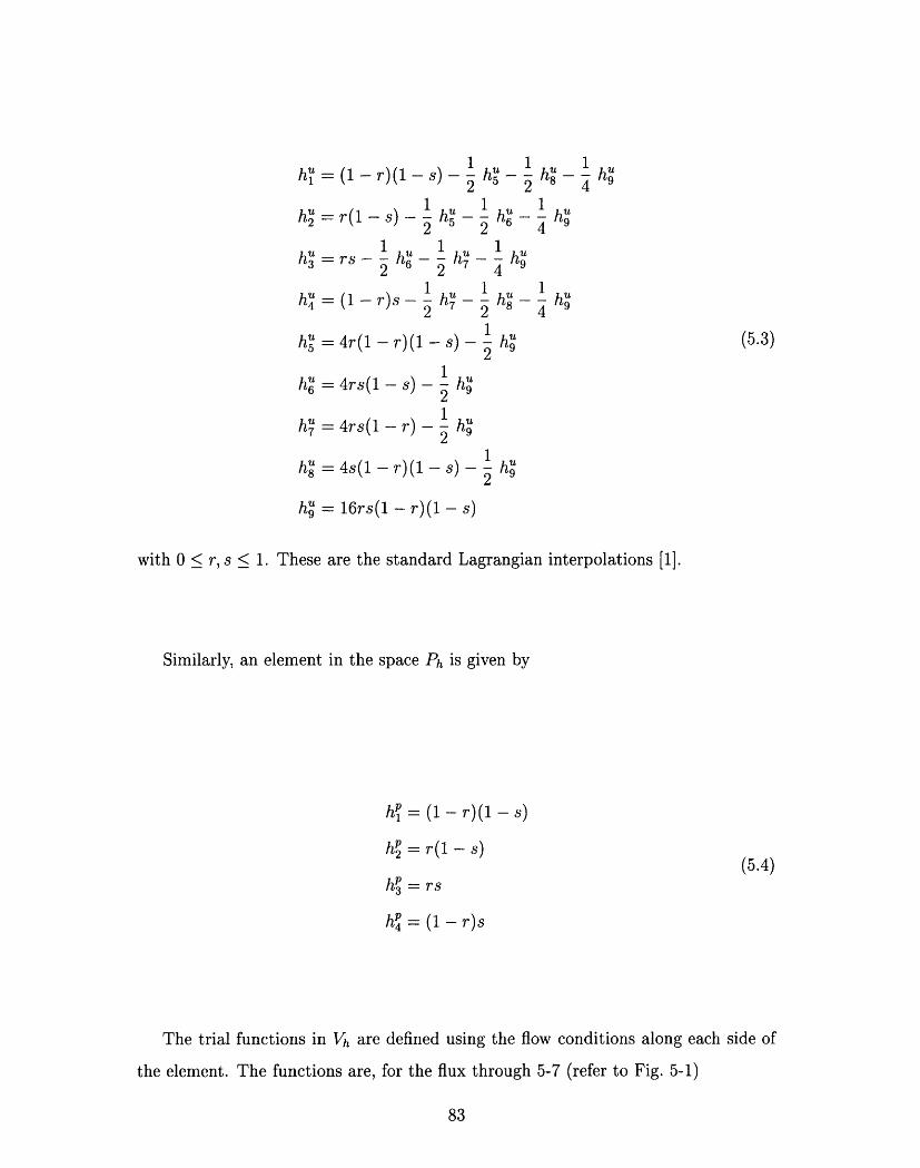
h (1 - r)(1 - s) - h -2

h= rs - h6-

h = (1 - r)s -

1 I

2 4

h7 -

1

9

h = 4rs(1 -

h = 4rs(1 -

1s) -2 h1r) -T) h

2

1

49(5.3)

1

9

hu = 16rs(1 - r)(1 - s)

with 0 < r, s < 1. These are the standard Lagrangian interpolations [1].

Similarly, an element in the space Ph is given by

hp = ( 1 - r )( 1 - s )

hp = r(1 - s)

hp = rs

hp = (1 - r)s

The trial functions in Vh are defined using the flow conditions along each side of

the element. The functions are, for the flux through 5-7 (refer to Fig. 5-1)

83

(5.4)

U h - hu8

U 1~~~h2 r(l - ) 2 -

1 U - h - h~

2 6

u = 4(I r)I -s)

hu = 4s(I - r) (I - s -8

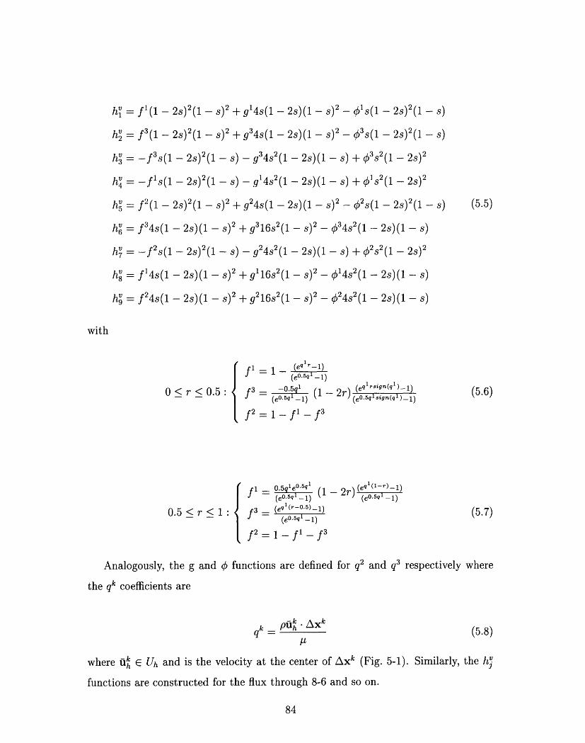
hv = fl(1 - 2s)2(1 - s)2 + g14s(1 - 2s)(1 - s)2 - qls(l - 2s)2(1 - s)

h = f 3 (1 - 2s)2(1 - s)2 + g3 4s(1 - 2s)(1 - s)2 - 3s(1 - 2 )2(1 - s)

hv = -f3 s(1 - 28)2(1 - S) - g34s2(1 - 2s)(1 - s) + 03 s2(1 - 2S)2

hV = -f1s(l - 2s)2(1 - s) - g1482(1 - 2s)(1 - s) + 1ls2(1 - 2s)2

hs = f 2(1 - 2s)2(1 - )2 + g24s(1 - 2s)(1 - )2 - 02s(1 - 2s)2(1 - s)

hv = f 34s(1 - 2s)(1 - )2 + g9316s2(1 - )2 - q034s2(1 - 2s)(1 - s)

hv = -f 2 s(1 - 2s)2(1 - s) - 924 -2(1 - 2s)(1 - s) + 02s2(1 - 28)2

hv = f'4s(1 - 2s)(1 - s)2 + g116s2(1 - s)2 - 014s2(1 - 2s)(1 - s)

hv = f24s(1 - 2s)(1 - s)2 + g216s2(1 - s)2 - 024s2(1 - 2s)(1 - s)

O < r < 0.5:

0.5 < r < 1:

{

{

fl = 1 - (eqlr1)

f3 = -0.5ql (1 -(eO.5ql- 1)

f2 = 1 - fl _ f3

flf3

= 0.5ql eo5q (1(e0.5q -1)

_ (eq l

(r- 0

5)_1)

- (eO5ql 1)

(5.6)- 2r) (eqlrsign(ql )-l)(eO5qlsign(ql )-1)

- (eql (1-r) _ 1)(eO.5q1-1)(5.7)

f2 = 1 - fl _ f3

Analogously, the g and b functions are defined for q2 and q3 respectively where

the qk coefficients are

qk =Uh Pi AxkAU

(5.8)

where fu E UJh and is the velocity at the center of Axk (Fig. 5-1). Similarly, the hj

functions are constructed for the flux through 8-6 and so on.

84

(5.5)

with

To demonstrate these functions in more details, the f, g and 0 functions are

shown in Fig 5-2 for three values ql = 10, q2 = 0 and q3 = 200 respectively. As it was

mentioned earlier, for the flux through 5-7 (Fig 5-1), fl, f 2 and f 3 are exponential

functions of ql and r as given in equations (5.6) and (5.7). Similarly, g and 0 functions

are exponential functions of q2 and r and q3 and r respectively.

for q = 10f,e- f

for q2 = 0

for q3 = 200

FluxL==> q2=0

q':=10

- 41

. ecb

1.0 4i functions

rnctions

Figure 5-2: The demonstration of f, g and functions for the flux through 5-7 forthe three different values of q = 10, q2 = 0 and q3 = 200

To demonstrate the hi functions, once again we consider that the flux is through

5-7 in Fig 5-1 and the hi trial functions are as given in equation (5.5): h is, for

85

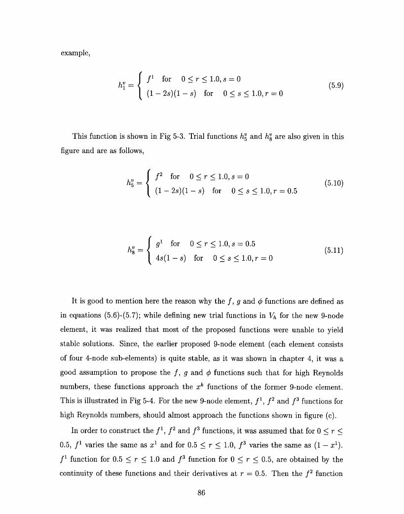
example,

f l for 0<r< 1.0, s=0 (

- (1 - 2s)(1 - s) for 0 < s < 1.0, r 0 (5=

This function is shown in Fig 5-3. Trial functions h5 and h are also given in this

figure and are as follows,

f 2 for 0 < r < l .,s0 (5.10)

n (1-2s)(1-s) for 0 < s < 1.0, r = 0.5

hv { gl for 0 < r < 1.0, s = 0.5 (511)

4s(1-s) for 0 < s < .0, r= 0

It is good to mention here the reason why the f, g and functions are defined as

in equations (5.6)-(5.7); while defining new trial functions in Vh for the new 9-node

element, it was realized that most of the proposed functions were unable to yield

stable solutions. Since, the earlier proposed 9-node element (each element consists

of four 4-node sub-elements) is quite stable, as it was shown in chapter 4, it was a

good assumption to propose the f, g and functions such that for high Reynolds

numbers, these functions approach the xk functions of the former 9-node element.

This is illustrated in Fig 5-4. For the new 9-node element, fl, f 2 and f3 functions for

high Reynolds numbers, should almost approach the functions shown in figure (c).

In order to construct the fl, f 2 and f3 functions, it was assumed that for 0 < r <

0.5, fl varies the same as x1 and for 0.5 < r < 1.0, f3 varies the same as (1 - xl).

f:L function for 0.5 r < 1.0 and f 3 function for 0 < r < 0.5, are obtained by the

continuity of these functions and their derivatives at r = 0.5. Then the f 2 function

86

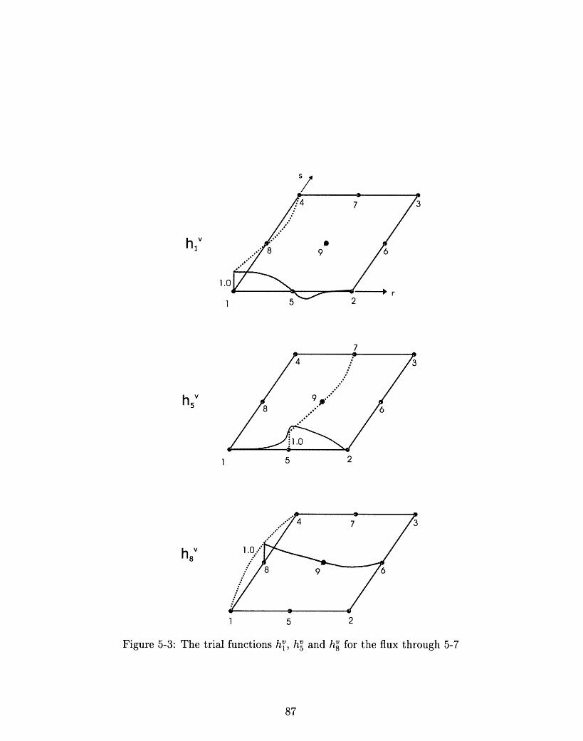
hlV

1.0

1

h5 V

1 5 2

h 8v

1 5 2

Figure 5-3: The trial functions h, h and h for the flux through 5-7

87

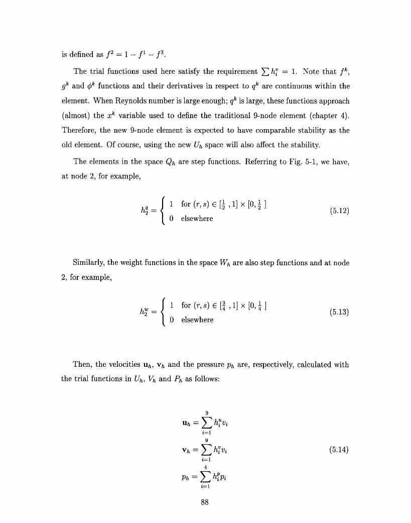
is defined as f2 = 1- f - f3 .

The trial functions used here satisfy the requirement E hj = 1. Note that fk,

gk and ok functions and their derivatives in respect to qk are continuous within the

element. When Reynolds number is large enough; qk is large, these functions approach

(almost) the xk variable used to define the traditional 9-node element (chapter 4).

Therefore, the new 9-node element is expected to have comparable stability as the

old element. Of course, using the new Uh space will also affect the stability.

The elements in the space Qh are step functions. Referring to Fig. 5-1, we have,

at node 2, for example,

1 for (r,s) E [ ,1] x [0, (5.12)hq

2 2 (5.12)0 elsewhere

Similarly, the weight functions in the space Wh are also step functions and at node

2, for example,

1 for (r,s) E [3 ,1] x [0, (5.13)

0 elsewhere

Then, the velocities Uh, vh and the pressure Ph are, respectively, calculated with

the trial functions in Uh, Vh and Ph as follows:

9

Uh = E h uvi

i=l9

Vh = E hVvi (5.14)i=-l4

Ph = Z hPii=l

88

4 7 3

(a) The earlier proposed 9-node element

1,0

(b) x and (1 -x') functions for the shown sub-element

1,0

(c) x' and (1 -x1) functions for the assemblage of two adjacent sub-elements

Figure 5-4: The earlier proposed 9-node element (consists of four 4-node sub-elements); x- and (1-x 1 ) functions are shown for one sub-element and the assemblageof two adjacent sub-elements for high Reynolds number flow when the flux is through5-7

89

where vi and Pi are the nodal velocity and pressure variables. As in chapter 4, the

flux is calculated with the interpolated values at the center of the sides of the control

volumes. Analogously, the corresponding linearized finite element matrix equations

are,

KVXV Kv V KP Av RVx Fv

Kvv v Kvv p Ivy = Rv - Fv (5.15)

KpvX KpvY 0 Ap 0 Fp

Similar to (4.24), AV, Avy, Ap, are the increments of velocity in x direction,

velocity in y direction and pressure with respect to the last iteration; Rvx and Rvy

are the discretized load vectors and Fv,, Fv, F contain terms from the linearization

process. Elements of the stiffness matrix are defined for the new 9-node element.

Using the back-substitution iteration method (in chapter 4, the full Newton-Raphson

iteration method was used) for a mesh of non-distorted elements, we get,

90

I6wYHU1r* vx H"vr* ds

2O HU Ir ds- ny -dzXd

JQfwx

Ox+ pny r

+Pf y

HUsI, Vy H v sI, dr

HU, s* dr)$

Or HU Is* dr19X r

KvYVV = --- E , aQw

s s HU l dsJ~.o s~w~ Oy

HUI,. vx Hv I,. ds + pny

rOx ( ,rlr dsOx-,/ny r

HUls, vy H v s dr

KVYP = E

Kvp = E

KPVZ = EQ,

Q,,

Oy

nzny

Oypnx s

Oxpn,

Y a

J•Ywy

AQWu

HPlr ds

HPl,S dr

HUIr. ds

H"I,. drJQq2

(5.16)

where Qw, and Qq are the control volumes for the velocity and pressure points respec-

tively (Fig. 5-5); all the integrals are calculated over the sides of the control volumes

91

K~vxv.: -f2w

Oy- Ln , x

19Y 2 -wY

Kvxvy = -- K,,,,=-CQt

Ox

KVVyV = I-I

Oy(pn

'98

Oy- O sX33

JQWX

o 2as

2 y9

HUSS* dr)

and subscripts x and y in aQ refer to the control volume sides in x and y directions;

nx and ny are the elements of the normal vector n and are either 1 or -1; the su-

perscript * indicates the flux is calculated with the interpolated values at the center

of the sides of the control volumes and HU, Hv and HP contain the trial functions

corresponding to Uh, Vh and Ph spaces.

o__ _A

for p3

S)w for p

Figure 5-5: Illustration of Qw and Qq; the control volumes of the velocity and pressurepoints respectively

5.2 Comparison of the new 9-node element with

the earlier published 9-node element

In this section the new proposed FCBI 9-node element, is numerically investigated

and compared to the former FCBI 9-node element which consists of four 4-node sub-

elements. The element is first tested for the driven cavity flow problem and then for

the S-channel flow problem.

92

RV

In both problems, when the Reynolds number is increased, the new FCBI 9-node

element has comparable stability as the former FCBI 9-node element. The reason

is that when the Reynolds number is large enough; qk is large and the fk, gk and

Ok functions (5.6-5.8) (almost) approach the xk variable used to define the earlier

published 9-node element (chapter 4). However, using the parabolic trial functions in

the Uh space for the new FCBI 9-node element slightly decreases the stability since

these functions have negative values as well within each element.

To study the accuracy and convergence of the new element, the same error norms

as section (4.5.2) are used; the L2 and H1 norms of the velocities and L2 norm of the

pressures.

12= E J(u - h) dxdy +over elements

21= E J(U-Uh)2 dxd +over elements

X (u -uh)2 x ddy +over elements o0

+ E t(U - Uh)Y, dxdy +over elements o

J(u- Uh)y dxdy (5.17)over elements

S J (U- Uh)y dxdyover elements

J(u- uh), , dxdy (5.18)ver elements

f(u - Uh) , dxdyuver elements

II P -Ph IIL2= E (P ph)2 dxdy (5.19)over elements

where h E Uh and Ph E Ph. Since the focus of this thesis is on the non-distorted ele-

ments, all the integrals are simply obtained using the Maple program (no numerical

integration).

In these equations, ( ), x and ( ), y are the x and y derivatives, (u - Uh)x

93

|U - Uh

U - Uh

and (u - Uh)y are the x and y components of (u - h) respectively where u is the

exact velocity and uh is the velocity obtained by the finite element solution. The

exact solution is the analytical solution and it is unknown for most of the fluid flow

problems. In these problems, the finite element solution obtained using the Galerkin

9-node element (with no upwinding) for a very fine mesh is assumed to be the exact

solution.

Note that for the earlier published FCBI 9-node elements in (4.5.2), Uh was the

space of bilinear functions within each sub-element and II u - Uh lL2 and 11 U- Uh IH1

norms were calculated over the sub-elements. Here, parabolic trial functions in Uh

space are defined within each 9-node element.

* The driven cavity flow problem (Re = 1000)

To demonstrate the solution errors in detail, the non-uniform mesh of 4x4 el-

ements (Fig.4.?), 8x8 and 16x16 elements are considered. The exact solution is

assumed to be the finite element solution obtained using the Galerkin 9-node element

(with no upwinding) for a uniform mesh of 64x64 elements. Figure 5-6 illustrates

that the 11 u - Uh [IL2 , 11 U - Uh fH1 and || p - Ph HlL2 norms converge when the mesh

is refined. In this figure, the solid and the dashed lines represent the solutions for the

new FCBI 9-node elements and the earlier published 9-node elements, respectively.

It is clear that the solution errors are smaller using the new FCBI 9-node element

but the rate of convergence is almost the same.

* The S-channel flow problem (Re = 100)

For the S-channel flow problem, consider the same mesh shown in Fig.4.? and 2

times finer and coarser meshes. Convergence curves for the velocity are given in figures

(5-7a) and (5-7b) for the L2 and H1 norms respectively. In figures (5-7c) and (5-7d),

we show the convergence curves for II p - Ph IIL2 and for I U - uh IIH1 + II - Ph IL2

In this figure, the solid and the dashed lines represent the solutions for the new FCBI

9-node elements and the former 9-node elements, respectively. When the mesh is

refined, velocity and pressure errors are smaller in the L2 norm for the new proposed

94

Original FCBI 9-node element ..............

New FCBI 9-node element

-1 -0.8 -0.6 -0.4 -0.2

log (h)

Fig 5.6 (a)

0

Original FCBI 9-node element ..............

New FCBI 9-node element

0

95

0

-0.2

-.0.3

-.0.5

-0.6-1.2

U

-0.05

-0.1

-0.15

-(0.2

-0.25

-0.3

-0.35

-0.4

-0.45

-0.5-1.2 -1 -0.8 -0.6 -0.4 -0.2

log (h)

Fig 5.6 (b)

Original FCBI 9-node element ..............

New FCBI 9-node element

0.2

-0.8 -0.6

log (h)

Fig 5.6 (c)

-0.4 -0.2

Original FCBI 9-node element ..............

New FCBI 9-node element

.f

-1 -0.8 -0.6 -0.4 -0.2

log (h)

Fig 5.6 (d)

Figure 5-6: Comparison of the new FCBI 9-node elements and the original FCBI9-node elements for the driven cavity flow problem (Re=1000). In this figure, the xcoordinate represents log h when h is the mesh size and the y coordinate for each caseis a) log 11u-uh11L2 , b) log 1 -Uh11H , c) log P-PhL2 d) log ( u UH1 + P-PhL2

IlUiIL2 ,UH1 IIPH

96

-1

-1.1

-1.2

-1.3

-1.4

-1.5

-1.6-1.2 -1 0

0

-0.05

-0.1

-0.15

-0.2

-0.25

-0.3

-0.35

-0.4

-0.45-1.2 0

9-node element, and the velocity errors are the same for the H1 norm. In addition, the

convergence curves for the L2 norm (for the velocity and the pressure both) display

a larger rate of convergence for the new 9-node element.

5.3 Comparison of the new 9-node element with

the Galerkin 9-node element

In this section the newly proposed FCBI 9-node element, is compared to the Galerkin

9-node finite element. The Galerkin 9-node finite element uses the 9 nodes for the

velocities and the 4 corner nodes for the pressure interpolations 2 . To compare the

accuracy and convergence of the new element and the Galerkin 9-node element, the

same error norms as in section (4.5.2) are used; the L2 and H1 norms of the velocities

and L2 norm of the pressures, and the same driven cavity flow and the S-channel flow

problems are considered.

In both problems, when the Reynolds number is increased, the new FCBI 9-node

element is more stable than the Galerkin 9-node element. However, in the cavity

flow problem, using the Galerkin 9-node element yields more accurate solutions with

a higher rate of convergence. Since our goal is to use a new 9-node FCBI element

together with the "goal-oriented error estimation" to control the error of the solution

in the structural response in the FSI problems, we want a 9-node element with much

better stability and comparable accuracy as Galerkin 9-node element. From the

numerical results presented in this section, it becomes clear that the new 9-node

elements do not obtain the solution as accurate as the Galerkin 9-node elements but

the solution is stable for much higher Reynolds numbers (than the Galerkin 9-node

elements), and accurate enough to be used to find the structural responses.

* The driven cavity flow problem

The same non-uniform meshes 4x4, 8x8, 16x16 and 32x32 elements used in (5.2)

are considered. Figure 5-8 shows the convergence of the 11 u - Uh L2 , 11 U - Uh H12Also referred to as the Taylor-Hood, Q9/Q4, or 9/4-c element [1]

97

-0.5

-1.5

-.1.5

-2

-2.5

Original FCBI 9-node element ..............

New FCBI 9-node element

-0.9 -0.8 -0.7 -0.6 -0.5 -0.4 -0.3 -0.2 -0.1 0

log (h)

Fig 5.7 (a)

1o8 ~...._- .:....-0.5 0

-1

Original FCBI 9-node element ..............

New FCBI 9-node element

-2

-2.5

-3-0.9 -0.8 -0.7 -0.6 -0.5 -0.4 -0.3 -0.2 -0.1 0

log (h)

Fig 5.7 (b)

98

n

I I~~j

0

-0.5 -

-1 -

-1.5

-2-0.9 -0.8 -0.7 -0.6 -0.5 -0.4 -0.3 -0.2 -0.1 0

log (h)

Fig 5.7 (c)

n R_...................

0-

-0.5

-1

-1.5 -

-2

Original FCBI 9-node element ..............

New FCBI 9-node element0.9 .Z-2--

_0. .o. ' 'O

of\G

-0.9 -0.8 -0.7 -0.6 -0.5 -0.4 -0.3 -0.2 -0.1 0

log (h)

Fig 5.7 (d)

Figure 5-7: Comparison of the new FCBI 9-node elements and the original FCBI9-node elements for the S-channel flow problem (Re=100). In this figure, the xcoordinate represents log h when h is the mesh size and the y coordinate for eachcase is a) log IIU-UhlL2 , b) log IIU-Uhl1 , c) log i-PhIIL2 , d) log (11U-UhHl ± IIp-Ph L2

IlUlL2 IIUIIH1 IIPIIL2 IlullH1 IIPIIL2 )

99

Original FCBI 9-node element ..............

New FCBI 9-node element

1

IY

I-I

and [I p - Ph [[L2 norms when the mesh is refined. In this figure, the solid and the

dashed lines represent the solutions using the new FCBI 9-node elements and the

Galerkin 9-node finite elements, respectively. From the convergence curves shown

in this figure we observe that the errors are larger using the new proposed 9-node

element. In addition when the mesh is refined, the Galerkin 9-node element has

higher rate of convergence. However, the Galerkin 9-node element only yields stable

solutions for low Reynolds numbers.

Table 5.1]. compares the stability of the new proposed 9-node element with the

Galerkin 9-node element. In this table, a non-uniform mesh 16x16 elements is used,

and the number of iterations required to solve the problem, is also shown for the

earlier proposed FCBI 9-node element.

To obtain the results given in this table, the Newton-Raphson iteration method is

used for the Galerkin 9-node element and the former FCBI 9-node element when the

back-substitution method is used for the new FCBI 9-node element. In this table,

(*) denotes that the iteration did not converge within the allowable 50 number of

iterations. This table is given for the convergence tolerance 10- 3. As it is clear, both

FCBI 9-node elements give more stable solutions than the Galerkin 9-node element.

Since our goal is to use a 9-node element together with the "goal-oriented error

estimation" to control the error of the solution in the structural response in the fluid-

structure interaction problems, we want an element that gives stable solutions for high

Reynolds numbers (more stable than the Galerkin 9-node element) with reasonable

accuracy (in a coarse mesh). The new proposed 9-node element is such an element

which yields stable solutions for higher Reynolds numbers. Although the errors are

larger for the new 9-node element, the accuracy of the solution is still reasonable to

obtain the structural response in the FSI problems.

In the case of using the Galerkin 9-node finite elements, the solution for the mesh

of 4x4 elements is not stable and therefore not given in the figure.

* The S-channel flow problem

For the S-channel flow problem, consider the same meshes as used in section (5.2).

100

...... : 0 .51

rkin 9-node element

FCBI 9-node element

-1 .4 -1.2 -1 -0.8

log (h)

Fig 5.8 (a)

;. . ..

-0.6 -0.4 -0.2 0

- -3--. 0.31

rkin 9-node element

FCBI 9-node element

-1.4 -1.2 -1 -0.8

log (h)

Fig 5.8 (b)

101

-0.6 -0.4 -0.2 0

U

-0.5

-1

-1.5

-2

-2.5

-3

-3.5

-4

V.;

0

-0.5

-1

-.1.5

-2

-2.5

-3

Fo

.

-1

-1.5

-2

-2.5

-3

-3.5

-4

-4.5

element

-1.4 -1.2 -1 -0.8 -0.6 -0.4 -0.2 0

log (h)

Fig 5.8 (c)

n1 x_U.D

0

-0.5

-1

-1.5

-2

-2.5

-3-1.4 -1.2 -1 -0.8 -0.6 -0.4 -0.2 0

log (h)

Fig 5.8 (d)

Figure 5-8: Comparison of the new FCBI 9-node elements and the Galerkin 9-nodeelements for the driven cavity flow problem (Re=1000). In this figure, the x coordi-nate represents log h when h is the mesh size and the y coordinate for each case is

a) log lu-uhlL2 7 b) log lu-cuhll. , c) l og P--Ph L2 d) log ( lu-hlHl + Ipl-p IL )

11uL2 guH loPgl L2 'ull'i 11P11L2

102

^_~- ~ ~ ~ . _ . ~ ~ ~ - . , . _ _ . ..... .

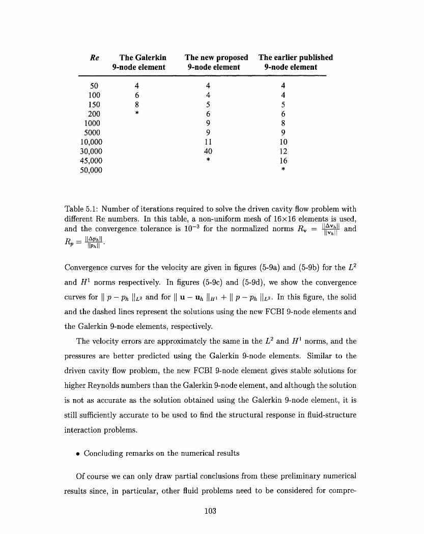
Re The Galerkin The new proposed The earlier published9-node element 9-node element 9-node element

50 4 4 4100 6 4 4150 8 5 5200 * 6 6

1000 9 85000 9 9

10,000 11 10

30,000 40 1245,000 * 1650,000 *

Table 5.1: Number of iterations required to solve the driven cavity flow problem withdifferent Re numbers. In this table, a non-uniform mesh of 16x 16 elements is used,and the convergence tolerance is 10-3 for the normalized norms Rv - IAvhill and

Ronvir c c e PhfI

Convergence curves for the velocity are given in figures (5-9a) and (5-9b) for the L2

and H1 norms respectively. In figures (5-9c) and (5-9d), we show the convergence

curves for 1 p - Ph IIL2 and for II u - Uh IIH1 + II P - Ph IL2. In this figure, the solid

and the dashed lines represent the solutions using the new FCBI 9-node elements and

the Galerkin 9-node elements, respectively.

The velocity errors are approximately the same in the L2 and H1 norms, and the

pressures are better predicted using the Galerkin 9-node elements. Similar to the

driven cavity flow problem, the new FCBI 9-node element gives stable solutions for

higher Reynolds numbers than the Galerkin 9-node element, and although the solution

is not as accurate as the solution obtained using the Galerkin 9-node element, it is

still sufficiently accurate to be used to find the structural response in fluid-structure

interaction problems.

* Concluding remarks on the numerical results

Of course we can only draw partial conclusions from these preliminary numerical

results since, in particular, other fluid problems need to be considered for compre-

103

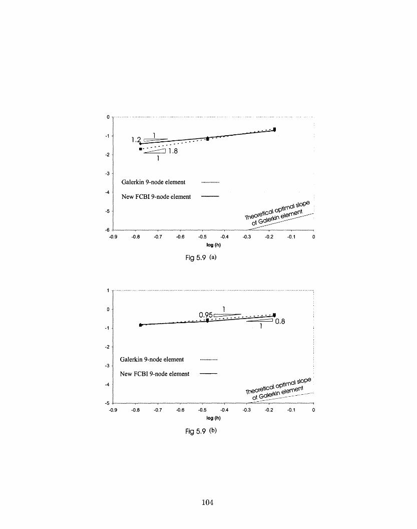
1

¶ ='';- 1.81

Galerkin 9-node element

New FCBI 9-node element

om Cr\l"eo,~e'~c° ...o e~eroe°~'I ¢

.9 -0.8 -0.7 -0.6 -0.5 -0.4 -0.3 -0.2 -0.1 0

log (h)

Fig 5.9 (a)

1..... ..... 5. .-

Oalerki 9- 1let0.8

Galerkin 9-node element *--.

New FCBI 9-node element

-4 0 o.3 -0.2 -0.1leoeIc : eeme ent .-

-0.4 -0.3 -0.2 -0. 1 0-0.9 -0.8 -0.7 -0.6 -0.5

log (h)

Fig 5.9 (b)

104

0

-1

-2

-.6-0

1

0

-.1

-2

-:3

-4

-5

_

1.2 c.

.. - -

1

Galerkin 9-node element

New FCBI 9-node element

'lheoretiGon elefiment- , , ,~~ , .r" ~ . . . . . .~. . . ----

-0.9 -0.8 -0.7 -0.6 -0.5 -0.4 -0.3 -0.2 -0.1 0

log (h)

Fig 5.9 (c)

. .... .................................................................................................................................................. ... .......................... ......... .... . . . . . .

Galerkin 9-node element ............

New FCBI 9-node element 1

0.9 ~ &

Geo~e'~e ).~ e~

-0.9 -0.8 -0.7 -0.6 -0.5 -0.4 -0.3 -0.2 -0.1 0

log (h)

Fig 5.9 (d)

Figure 5-9: Comparison of the new FCBI 9-node elements and the Galerkin 9-node

elements for the S-channel flow problem (Re=100). In this figure, the x coordinaterepresents log h when h is the mesh size and the y coordinate for each case is a)

log lu-u lL2 , b) log lu-l1 , C) log JP-PhjjL2 d) log ( i-UlH1 + I-PL )2HJuHL,2 " J1uJH1 'l1P112 ' JuJH1 1JP1IL2

105

0-

-1 -

-2-

-3

-4 -1

-5

-6

-7-

o0-

-1 -

-2 -

-3

hensiveness.

From these numerical results, the new proposed FCBI 9-node element appears to

predict the solution more accurate than the earlier published FCBI 9-node element.

For the S-channel flow problem, the convergence curves display a larger rate of con-

vergence using the new 9-node element. In addition, the errors are larger using the

new 9-node element than using the Galerkin 9-node element but still accurate enough

to be used together with the "goal-oriented error estimation" to control the error of

the solution in the structural response in the fluid-structure interaction problems ( for

"goal-oriented error estimation" we want a 9-node element that with reasonable accu-

racy gives stable solutions for high Reynolds numbers, however the Galerkin 9-node

element is only stable for low Reynolds numbers).

106

Chapter 6

Linking FCBI to CIP method

(CIP-FCBI)

Hydrodynamics equations presented with partial differential equations are usually

hard to solve numerically. For example, in problems with discontinuity one must

deal with the sudden change of the values or discontinuity in solving these equations.

Although there has been progress in numerical analysis and computing technology,

various proposed methods are complicated, require much computational effort and are

applicable only for specific problems. Therefore, there is still interest in developing

more effective methods for solving hydrodynamics equations numerically.

The Cubic-Interpolated Pseudo-particle (CIP) method was introduced by T.Yabe

et al. in 1991 [26], [17]. In this method, a cubic polynomial is used to interpolate

the spatial profile of the value f and its spatial derivative Vf. The spatial derivative

itself is a free parameter and satisfies the master equation for the derivative. After

the values f and Vf are found, the same values for the next time step are simply

calculated by shifting the cubic polynomial.

The CIP scheme is a very stable finite difference technique that can solve gen-

eralized hyperbolic equations by the 3rd order of accuracy in space. For nonlinear

problems, the CIP scheme splits the hyperbolic equation into two phases; the non-

advection phase and the advection phase. In each time step, after the non-advection

phase is solved by the finite difference method, the CIP method is applied to the ad-

107

vection phase. This method has been applied to various problems such as solving the

Korteweg-de Vries equation and the one-dimensional and two-dimensional shock-tube

problems.

The CIP-CUP method (CIP-Combined Unified Procedure) was introduced by

T.Yabe et al. to solve complex compressible and incompressible fluid flow prob-

lems [25], [27]. This method is a pressure-based semi-implicit solver for the Euler

equations or the Navier-Stokes equations of fluid flows. The CIP-CUP method solves

the non-conservative form of the governing equations in three phases; the convection

phase, the remaining phase and the acoustic phase. The acoustic part is solved im-

plicitly by the CUP method while the convection part is solved explicitly by the CIP

method. However, at the interface of different fluids in composite flows, or for fluid

flow structure interaction problems at the interface of the fluid and structure, there

will be oscillation and diffusion in the solution. The reason is that the physical quan-

tities (the material properties) and consequently the sound speeds have large changes

at the interfaces which causes problems in the numerical solution.

In section 1, a review of the CIP method is given. Then, in order to solve the

Navier-Stokes equations, the CIP scheme is linked to the finite element method (CIP-

FEM) and the FCBI scheme (CIP-FCBI), in sections 2 and 3 respectively.

6.1 CIP method

In order to do numerical simulations, the continuous media should be discretized. The

goal of the numerical algorithms is not to lose information inside the grid cell between

the digitized points. However, most of the proposed numerical schemes fail to take

care of the real solution inside the grid cell and in order to have a high resolution,

the grid cells should be very small. The CIP method constructs a solution inside the

grid cell which is sought close to the real solution of the given equation. We explain

the strategy of the CIP method by using the linear advection equation,

Of Of+ u =O0 (6.1)at + Ox10

108

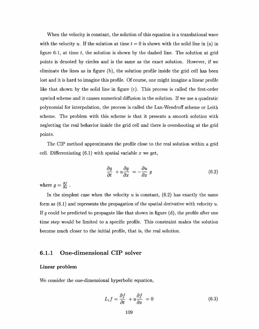
When the velocity is constant, the solution of this equation is a translational wave

with the velocity u. If the solution at time t = 0 is shown with the solid line in (a) in

figure 6-1, at time t, the solution is shown by the dashed line. The solution at grid

points is denoted by circles and is the same as the exact solution. However, if we

eliminate the lines as in figure (b), the solution profile inside the grid cell has been

lost and it is hard to imagine this profile. Of course, one might imagine a linear profile

like that shown by the solid line in figure (c). This process is called the first-order

upwind scheme and it causes numerical diffusion in the solution. If we use a quadratic

polynomial fIor interpolation, the process is called the Lax-Wendroff scheme or Leith

scheme. The problem with this scheme is that it presents a smooth solution with

neglecting the real behavior inside the grid cell and there is overshooting at the grid

points.

The CIP method approximates the profile close to the real solution within a grid

cell. Differentiating (6.1) with spatial variable x we get,

Og Og Ou+ U g - 9 (6.2)

At x = x

where g = -

In the simplest case when the velocity u is constant, (6.2) has exactly the same

form as (6.1) and represents the propagation of the spatial derivative with velocity u.

If g could be predicted to propagate like that shown in figure (d), the profile after one

time step would be limited to a specific profile. This constraint makes the solution

become much closer to the initial profile, that is, the real solution.

6.1.1 One-dimensional CIP solver

Linear problem

We consider the one-dimensional hyperbolic equation,

Lf af afLl f = af+uf-0 (6.3)ot Ox

109

u At1I->1

U - '

fi f-I i

I T

ti -fi +1

I i

Xi-l Xi Xi+l Xi+2

(a)

fi +1

Xi. I Xi Xi+l Xi+2 X

(C)

Xi.l Xi Xi+l Xi+2

(d)

Figure 6-1: The principle of the CIP method. (a) The initial profile and the exactsolution (b) The exact solution at the grid points (c) Linear profile between the gridpoints (d) The spatial derivative in the CIP method

110

Of-+

T XX Xi-I

IXi Xi+l

TXi+2 X

(b)

fi -1

. _ . . h

_ e

-

I

where the value of f is given at grid points xl,...,xi,... at time t - At. Within each

cell (k) bounded by nodes i and i + 1, f is interpolated using a cubic polynomial such

as,

Fk(X) = [ (aiX + bi)X + fi' ]X + fi (6.4)

where X = x - xi and fi' denotes the spatial derivative of f at point i.

In the CIP method the spatial derivative of f is itself a variable and should satisfy

the spatial derivative of the master equation (6.3).

L1(aOf) = + af (6.5)at + z u Ox

The values of f and f' are known at all the grid points and in order to find f

within each cell, the coefficients ai and bi should be determined. For the grid cell (k)

located between grid points xi and xi+l, these coefficients are found by the continuity

of f and f' at point i + 1.

fi = Fk(X = Ax) = [ (aix + bi)Ax + -f ]Ax + fi(6.6)

f O Fk(X = Ax) = 3aiAx2 + 2biAx + (6.6)

where Ax = xi+l - xi.

Then these coefficients are as follows,

(f'i + f' i+ + 2(fi - fi+l)ai = +X2 4 -A2 A3 (6.7)

(2f'i + f'i+l) 3(fi+l - fi)Ax + Ax2

Once ai and bi are known in terms of fn and fIn ( f and f' at time t - At), the

value of f n+l is simply given by shifting the cubic polynomial and its derivative. For

111

the linear advection equation with u = constant, equation (6.5) is equivalent to (6.3)

and fn can also be used to estimate fn+l. Thus,

fn+l = F(xi - uAt) = [(ai + bi)~ + f] + fifn+l dF(xi - unt) (3ai + 2bi(6.8)

dx

where = --uAt.

This expression is derived for u < 0. For u > 0, we obtain a similar expression

but we should replace Ax by -Ax and i + 1 by i - 1 in (6.7).

This scheme is called CIPO and has been found reasonably accurate for many

problems including nonlinear problems. However, for problems with discontinuous

fronts, the spatial derivative is not continuous at the front and it has different values

f'R and f'L for the right side and left side of the front respectively. Therefore, some

improved CIP schemes have been proposed, i.e. CIP1 and CIP2.

Non-linear problem

Consider the hyperbolic equation,

af + (fu) =9 (6.9)At +Ox

where the advection velocity u and the source term g can be a function of f. This

equation can be rewritten as,

aŽf +uaf =G=g-f at (6.10)at Ox Ox

As it was explained before, f' should satisfy the spatial derivative of the master

equation (6.10) as,

Of' Of' = uua =U G' -f'l (6.11)

In order to solve (6.10) and (6.11), the CIP scheme splits the problem into two

112

phases; the non-advection phase and the advection phase. The non-advection phase

is solved by a finite difference scheme while the advection phase is solved by the CIP

solver.

* Non-advection phase

The equations to be solved are,

Oaf )Vat (1

oaf t (1)

= G'- fOuOx

(6.12)

The first equation is simply solved using finite differencing

f* = f + GAt (6.13)

where the superscript (*) stands for the time after one step in the non-advection

phase.

The second equation in (6.12) can be solved again by finite differencing the equa-

tion or by finding ff in terms of G' from equation (6.13). Thus we have,

(fil* - f) In

At(fil - -Ni+1 + fi1)

2AxAt_n (Un+1 -Un 1)- fi 2Ax

2Ax

After f* and f'* are found, they will be taken to the advection phase.

* Advection phase

The equations to be solved are as follows,

afatOafat

(2)

) (2)

Of+ u

Of'+ u) ax

=0(6.15)

=0

113

(6.14)

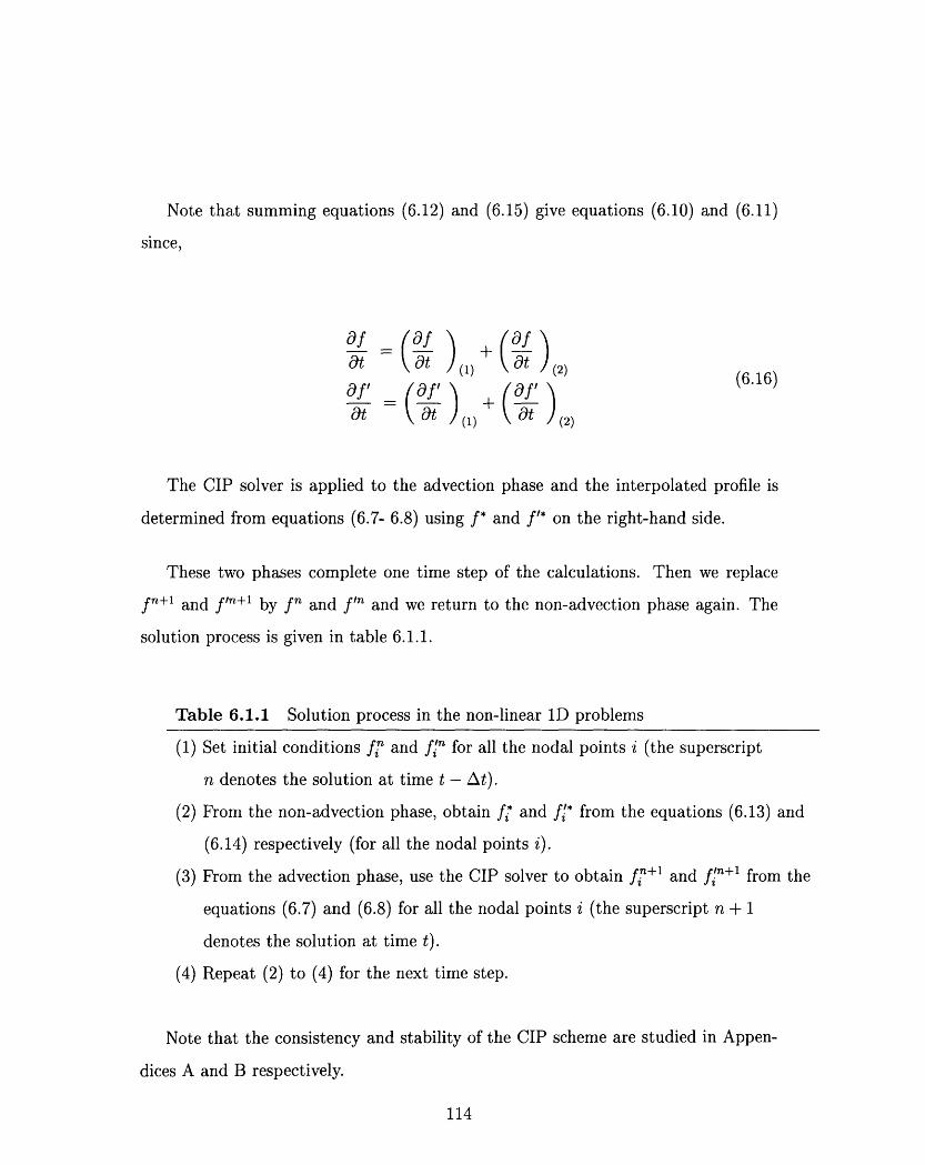
Note that summing equations (6.12) and (6.15) give equations (6.10) and (6.11)

since,

of of af + ,fat a )(1) (2)aft af )° (aft )° (6.16)Gt , t (1) (2)

The CIP solver is applied to the advection phase and the interpolated profile is

determined from equations (6.7- 6.8) using f* and f'* on the right-hand side.

These two phases complete one time step of the calculations. Then we replace

fn+l and f +l by fn and f'n and we return to the non-advection phase again. The

solution process is given in table 6.1.1.

Table 6.1.1 Solution process in the non-linear 1D problems

(1) Set initial conditions f and fln for all the nodal points i (the superscript

n denotes the solution at time t - At).

(2) From the non-advection phase, obtain fi* and f* from the equations (6.13) and

(6.14) respectively (for all the nodal points i).

(3) From the advection phase, use the CIP solver to obtain fin+1 and f+l from the

equations (6.7) and (6.8) for all the nodal points i (the superscript n + 1

denotes the solution at time t).

(4) Repeat (2) to (4) for the next time step.

Note that; the consistency and stability of the CIP scheme are studied in Appen-

dices A and B respectively.

114

6.1.2 Two-dimensional CIP solver

For simplicity we use a rectangular grid with spacing Ax and Ay and grid points

(i, j), (i + 1, j), (i + 1, j + 1) and (i, j + 1). We consider a two-dimensional hyperbolic

equation as follows,

af Of Ofot Ox Oy

(6.17)

When u < 0 and v < 0, we interpolate f(x, y) with a cubic polynomial within a

grid cell as,

Fi,j(x, y) =

where X = x:- xi,j, Y

the value of f is known

only nine parameters A

[(Ali,iX + A2ijY + A3i,j)X + A4i,jY + afi,j]X

+[(A5i,jY + A6i,jX + A7i,j)Y + aOfi,j]Y + fi,j(6.18)

= Y- Yij and aOf and ayf are f and C respectively. If

at all grid points, fi,j for i = 1,..., imax and j = 1,... ,jmax,

1, ... , A7, Oxf and Oyf need to be determined.

In the CI:P method, the first spatial derivatives should satisfy the derivative of the

master equation and thus we have,

af,xOt

Of,y

Ot

+ U Of xxOf,

+ u-x

+ v Of'y

OyOy

du av= fg - f'X f'OxOu Ov

= ay - f - f f,yay ayd

(6.19)

If aOf and ayf are known at all grid points, we only need to determine the co-

efficients A1, ... , A7. There are different two-dimensional CIP solvers based on the

assumptions made to find these coefficients. For the choice of having a continuous f

at grid points (i + 1,j), (i,j + 1) and (i + 1,j + 1) and continuous Oxf and Oyf at

grid points (i + 1, j) and (i,j + 1) we obtain,

115

Ali,j = [-2di + x(fi+l,j + fi,j)A]/Ax 3

A2i,j = [A8i,j - oadjAZx]/xzXy

A3ij = [3di - 0x(f+l,j + 2fi,j)Ax]/Ax2

A4i,j = [-A8i,j + OxdjAx + ydiAy]/AxAy (6.20)(6.20)

A5i,j = [-2dj + dy(fij+l + fi,j)Ay]/AY3

A6ij = [A8i,j - OydiAy]/AxAy2

A7i,j = [3dj - y(fi,j+l + 2fi,j)Ay]/Ay 2

A8ij = fi,j - fi+l,j - fi,j+l + fi+l,j+l

where di = +l,j- fi,j and dj = fi,j+l - fi,j. These equations are for u < 0 and v < 0.

For u > 0, we must change i + 1 to i - 1 and Ax to -x. Similarly for v > 0, j - 1

and -Ay are used instead of j + 1 and Ay.

We split equations (6.17) and (6.19) into two phases; the advection phase and the

non-advection phase. After the non-advection phase is solved by a finite difference

scheme, the CIP solver is applied to the advection phase.

* Non-advection phase

The equations to be solved are,

(f ))at )

afft ) =Oxg) f, a auz - - av (6.21)

at )n,=auu9 -ay - f' ay

where the subscript (1) in these equations denotes the non-advection part of the time

derivatives o/: oaf, and f' ,Ot a t at

116

These equations are solved using a finite difference method and the quantities f,

cOf,; and Of,y are advanced as

fh = ffi + g9i,j At

= fif+. 1 ,j- fi*-1 ,j - f l ,j + fin j2Ax

nq n (Ui+l,j - Ui-l,j)At n n (Vi+l,j- V-Ji,j 2ZX -V- YJi,j

f j- j-1- fij+1 + fTi,-1y f;-3,- 2y f

n xf, (Uij+l - ui,j-1)ht n (Vij+ii j 2Ay - Oyfj

(6.22)2Ax

2Ay

where the superscript (*) stands for the time after one step in the non-advection

phase. After f*, Oxf* and Oyf* are found, they will be taken to the advection phase.

* Advection phase

The equations to be solved are as follows,

Of UOfat (2) + x+( Ofa N Of, at /(2) ax

at )(2) Ox

Ofv~ =0

+V Of,Oy

+V fyay

=0 (6.23)

=0

where the subscript (2) in these equations denotes the advection part of the time

derivatives f ofx, and f, . Note that summing the non-advection equationst' at Ot

(6.21) and the advection equations (6.23) give the governing equations (6.17) and

(6.19) since,

117

- Vi-I'j)At

of af A xa

af, af.' + a ,,, (6.24)At at (l) (at /(2)aIVY at)(1 +( at 2(4,at at (1) + t (2)

The CIP solver is applied to the advection phase; coefficients A1,..., A7 are de-

termined from equations (6.20) and after a short time step At we update f and its

spatial derivatives as,

fin+l = F,( - uAt, yi,j - vAt)

afijl = F,j(xij - uat, yi,j - vt) (6.25)

ayfinj+l = yi,j(xi,j - uAt, Yi,j - vAt)

To follow the calculations for the next time step, we replace fn+l, &af n +l and

0yfn+l1 by f, aOfn and ayfn and we start from the non-advection phase again.

The two-dimensional solver described here is for the choice of having a continuous

f at grid points (i + 1, j), (i, j + 1) and (i + 1, j + 1) and continuous 9xf and ayf at

grid points (i + 1, j) and (i, j + 1). Based on the assumptions made, there are some

other two-dimensional solvers.

Type-A solver interpolates f within a grid cell as,

F(x, y) = C3,oX3 + C2,0X2 + Oxfi,jX + fi,j + C,3Y (6.26)(6.26)

+ Co,2Y2 + yfijY + C2,1X2y + C1,1XY + C1,2XY2

where the C coefficients are determined from continuity of f at grid points (i, j),

(i + 1, j), (i, j + 1) and (i + 1, j + 1) while axf and dyf are continuous at grid points

118

(i,j), (i + 1,j) and (i,j + 1).

In order to develop a more accurate interpolation, we consider the continuity of

aOf and ayf at the grid point (i + 1, j + 1) in addition to the above conditions. This

interpolation is called Type-B and the interpolation function is expressed as follows,

F(x, y) -= C3,0X3 + C2,oX2 + eOfi,jX + fi,j + CO,3Y3 + Co,2Y2 + Oyfi,jY

+C3,1X 3y + C2,1X 2y + C1,2XY 2 + C1,1XY + C1,3XY 3

where the C coefficients are found from the continuity of f, aOf and Oyf at grid points

(i,j), (i + 1, j), (i,j + 1) and (i + 1,j + 1).

6.1.3 The CIP solver for compressible and incompressible

flows

Different CIP solvers have been proposed for the compressible and incompressible

fluid flows. Among these solvers, we present the most powerful one; the CIP-CUP

(Cubic Interpolated Propagation / Combined Unified Procedure) method [25], [27].

The CIP-CUP method is a semi-implicit solver that considers the governing equa-

tions of fluid flow as follows,

Op + u+u Vp = -pV uatOu V Vp F- +uVu =-- + (6.28)At P P

-pt +uVp=-pC2V.u

where p is the density, u is the velocity vector, p is the pressure and C, is the local

sound speed. For the Navier-Stokes equations, F contains viscosity effects, surface

tensions and external forces. For the Euler equations, there is no viscosity effect and

F only contains the surface tensions and external forces.

The CIP-CUP solver splits the problem into three different parts; the convection

119

part, the acoustic part and the remaining part. The convection part is solved by the

CIP method, the acoustic part is solved by the CUP method while the remaining

part is solved by a finite difference scheme or a finite volume method.

* The convection part

The equations to be solved are,

(&uc +u Vp=0at )(C, P

u (c)+uVu 0 (6.29)

ap +u Vp=O0at()where the subscript (c) denotes the convection part of the time derivatives.

The CIP solver explained in (6.1.2) is used to solve the convection part. We also

need to update the spatial derivatives of quantities p, u and p before we proceed to

the remaining part.

* The remaining part

The remaining part is governed by the equation,

( at ) Fr) = P (6.30)

where the subscript (r) denotes the remaining part of the time derivative term u

For the Navier-Stokes equations, F contains viscosity effects, surface tensions and

external forces. For the Euler equations, there is no viscosity effect and F only

contains the surface tensions and external forces. This equation can be solved by a

finite difference scheme or a finite volume method. After the velocity is updated, we

proceed to the acoustic part.

* The acoustic part

120

The governing equations of the acoustic part are,

at (a)

(at )(a) P (6.31)

at (a) PCV

where the subscript (a) denotes the acoustic part of the time derivatives. Note that

summing the governing equations of the convection part, remaining part and the

acoustic part yields the equations (6.28) since,

at (c) + at (a)= + d- - u (6.32)

ap (P + Pat tkatJ(c) k at (a)

These equations are solved by the CUP method, which is an implicit finite differ-

ence method. Discretizing the time derivatives on the left hand side of these equations

and estimating the right hand side for the future values (values to be found at the

end of this phase), we obtain

pn+l p*-- p*V·Un+lAt

Un + l - U* Vp n + l

(6.33)At P*

n p = - * C,*2 V. Un+At

where n is the number of the time step, At is the time interval, and the quantities

with the superscript (*) are the values after solving the convection and the remaining

121

parts. At each time step At, the acoustic phase should be solved after the other

phases since at the end of this phase, we satisfy the divergence-free condition for the

velocity in incompressible fluid flows.

In equations (6.33), the velocity, the pressure and the density at time n + 1 are

dependent. In order to find the pressure, we take the divergence of the second equation

and substitute it into the third equation. The pressure equation will then be,

P7,1+1 - * Vp n +lpl = -p* C V * u+* * C2 At V (6.34)At p*

After we find pn+l, Un+1 is obtained from the second equation of (6.33). Also, the

density is updated explicitly by

pn+l _ p*n1 = p* +P (6.35)

For incompressible fluid flows, the sound speed C, is infinite, and the pressure

equation (6.34) is reduced to

Vp n+l V U*V * (6.36)

P* At

Therefore, CIP-CUP method is applicable to both compressible and incompress-

ible fluids.

Calculation of pn+l, un+l and pn+l completes one time step of the CIP-CUP

method. For the next time step, we could repeat the calculation from the convection

part using above values as initial values. The solution process is given in table 6.1.3.

122

Table 6.1.3 Solution process in the CIP-CUP method

(1) Set initial conditions pi, u and pi and their spatial derivatives for all the

nodal points i (the superscript n denotes the solution at time t - At).

(2) From the convection phase use the CIP solver to get Pi, fii and Pi and their

spatial derivatives (for all the nodal points i).

(3) From the remaining phase, use a finite difference method to get pi, u and p*

and their spatial derivatives for all the nodal points i (p* = Pi*, P = Pi).

(4) From the acoustic phase, get p+ 1 , u +1 and pn+1 and their spatial derivatives

from the equations (6.33)- (6.35) for all the nodal points i (the

superscript n + 1 denotes the solution at time t).

(5) Repeat (2) to (5) for the next time step.

6.2 Linking the finite element method to the CIP

method

The CIP method was originally proposed for the finite difference method; both the

convection phase and the non-convection phase are solved using the finite difference

method. However in some problems, satisfying the boundary conditions for the in-

compressible Navier-Stokes equations is easier using the finite element methods. In

addition, in problems for which the domain is complicated and mesh grading is re-

quired, the finite difference methods are not as flexible as the finite element methods.

The CIP method is here extended for use in the finite element method and the

finite element; shape functions for the third order interpolation are introduced in [24],

[16]. This shape function is defined by the product of the linear shape function and

a new second. order shape function. In this chapter, these functions are used to solve

the two-dimensional incompressible Navier-Stokes equations.

6.2.1 The governing equations

The non-dimensional continuity and momentum equations are written as,

123

Vu=Ov u = 1Ou (6.37)ot + (u. V)u = -Vp + R V2u

where u, p and Re are the velocity vector, pressure and the Reynolds number respec-

tively. External force is not considered here.

The shape function for the third order interpolation function in CIP-FEM is de-

fined for the velocity u and its derivatives. Therefore, we need the spatial derivatives

of the momentum equation as follows,

Oux 1 V2- + (u . V)u = -(u/. V)u - Vp + uV2UaO~~uy ~~ R 1 (6.38)

atY + (u V)u = -(uY. V)u - Vp + R V2UY

where the subscripts x and y show the derivative in each direction.

We split the governing equations into an advection phase, a non-advection phase

and the Poisson equation of pressure. The advection phase is solved by the CIP

method (CIP-FEM), the non-advection phase by the Galerkin method, and the Pois-

son equation by the simultaneous relaxation method of the GSMAC (generalized

simplified marker and cell) method [18].

* The advection phase

The governing equations of the advection phase are,

u-u, + (un V)u =

u- + (u, . V)u = (6.39)At

ly-U Y + (un. V)un = At he solution at time t

where the superscript (n) stands for the solution at time t - At and the superscript

124

(^) stands for the solution after one step in the advection phase.

The CIP-FEM is applied to discretize and solve these equations. First, we describe

the CIP method. Considering the advection equation for a potential q,

90 + u V = (6.40)

The solution at time "t" is approximated as,

O(xi, t) q (xi - udt, t - dt) (6.41)

where xi denotes the grid point where 0 is given. The start point x = xi - f udt

becomes the grid point at the next time step. x,, is called the advection distance

and should be calculated along the particle path. However, the exact value of this

distance is difficult to obtain and it is approximated explicitly as,

Ax = xi -x* = u At (6.42)

In order for this approximation to be close to the exact value, At must be suffi-

ciently small..

In the CIP method, the potential is interpolated using the third order shape

functions, and these functions are defined for the system of coordinates -7. Since the

start point x, is obtained in the x-y coordinate system, we find the corresponding C,

and q7* for this point.

The shape function then is defined as,

q(, 7) = Z h(, r)[G.(, 7) + E.a(, 1)(/)a] (6.43)a

where ha is the conventional linear shape function, and Ga and Ea are new shape

functions that are second order and linear respectively.

For the element shown in figure 6-2, these functions are as follows,

125

hi = (1 - 7)(- 41

E2 = (e-i)

E3 = ( + 77)

41h4 = - (- + 77)

2

2

(6.44)

(6.45)

772)[O701 + 01]G1 = 2(1 - 2)[p1 + 01] + (1 -2 2

G2 = 2 (-1 + [2)[0 2 - 2] + (1 - 772 )[,7q2 + 2]

1 1(_ - 1 + rl )[O_1 + - q2G3 = 2 (-1 + ± 2)[aq03 - 3] + (-1 + 2)[73 - 3]

G = (1 _ 2)[O4 + ± 4] + (-1 + 772)[74 - 4]2 2

(6.46)

Using the CIP-FEM, the velocity u and its derivatives are updated for the time

"t" ( fi, fix and fly). These values are then taken to the non-advection phase.

* The non-advection phase

The governing equations are as follows,

126

4

1

3

2

2

Figure 6-2: The 4-node element used in the finite element discretization

U-U -p 1 2un

At Reu n +l - fix 1t = -(un V)un- VPln+l + v 2u n

Uy+1 - y up+ 1AtYYR

(6.47)

In order to avoid considering the pressure derivatives px and py as nodal variables

and updating them for each time step in the second and third equations, these terms

are replaced by the velocity terms from the first equation. Then, the second and third

equations are written as,

zt U= (Ux .V)un + ( At )At =+ ( At

t = (u. V)u + ) (6.48)

The non-advection phase is discretized by the Galerkin method. For the 4-node

element shown in figure 6-2, we use the four corner points to interpolate the velocity

when the pressure is constant within each element. Then the velocity u and its

derivatives in (6.47- 6.48) are replaced by

127

to

AL~

... . .. ... 4

I

-

4

u = E hiuii=1

4

U = E hxiuii=1

4

u = E hyiuii=1

(6.49)

After discretization by the Galerkin method, the first equation in (6.47) and equa-

tions (6.48) are written respectively as,

Mij ( f, ):.- =-Ai U + A, I)Mi At ujM,-fi U n+_ -

At j ) At

where p presents the constant pressure within the element, the lower subscripts i and

j show the local node numbers and superscript n is the time step number. Except

for the first term on the right-hand side of the second and third equations, repeated

subscripts mean summation. The matrices Mij, Ci, Aij and Dij are the mass matrix,

the gradient matrix, the advection matrix and the diffusion matrix respectively and

are written as,

Mij = hi hj dQe

Ci Vhi dQ

Aj = hi Vhj dQVh

Dij = Vhi Vhj dQe

(6.51)

128

(6.50)

where Si contains the boundary terms. Note that the Mij matrix shown here is the

consistent mass matrix. We can use the lumped mass matrix instead and replace Mij

by Mij in equations (6.50). For a non-distorted mesh, the Mij matrix is the same

for all the elements and therefore the assemblage will be easier. Note that in the

traditional finite element methods (solution is dominant by the stiffness matrix), the

lumped mass matrix is preferred since using the lumped mass matrix instead of the

consistent one, reduces the numerical operations for the solution significantly.

In the non-advection phase, first the velocity ft is obtained from the first equation

in (6.50), then the divergence of the velocity, V fi, is calculated. The simultaneous

relaxation method is used to satisfy the continuity equation (V fii = 0) and to modify

the velocity fu. This method is explained later on in this section.

After the simultaneous relaxation method has been applied, we find the modified

velocity un+'l and pressure pn+l. The velocity un+l is then used in (6.50) to obtain

un+1 and uy+1 . The calculations for one time step are complete now and for the next

time step, we take the values un+l, pn+l, U~n+l and Uy+1 to the advection phase and

we repeat the calculations for the new time step.

* The simultaneous relaxation method

This method is used to satisfy the continuity equation V fi = 0. After obtaining

fi in the non-advection phase, this velocity is modified as follows,

V2q(m) = V . i(m)

p(m+l) = p(m) + /(m)/At (6.52)

fU(m+1) = ~f(m) _ VO7(m)

where the superscript m represents the repeat level and b is the velocity potential.

The initial values are defined as,

129

f (o) =

(6.53)p(O) = pn

We first calculate the divergence of the velocity fu, then we obtain the velocity

potential 0 from the first equation in (6.52). Using the second and third equations,

the velocity and pressure are modified. We repeat the calculations until the velocity

fi satisfies the continuity equation; then we have,

un+l = U(m+l)(6.54)

pn+l p(m+l)

The solution process is given in table 6.2.1.

Table 6.2.1 Solution process in the CIP-FEM method for incompressible flows

(1) Set initial conditions un and the spatial derivatives ux and un for all the

nodal points (the superscript n denotes the solution at time t - At).

(2) From the advection phase use the CIP solver to obtain 1f and the spatial

derivatives fix and fly for all the nodal points using equations (6.43)- (6.46).

(3) From the non-advection phase, use the Galerkin method to obtain fi from

the first equation in (6.50).

(4) From the simultaneous relaxation method, obtain the velocity potential q

and the modified velocity and pressure from the equations (6.52). After

repeating calculations in this step and satisfying the equation V fi = 0,

obtain u n+l and pn+l

(5) From the non-advection phase, obtain the spatial derivatives u+1 and uyn+

from the second and third equations in (6.50).

(6) Repeat (2) to (6) for the next time step.

130

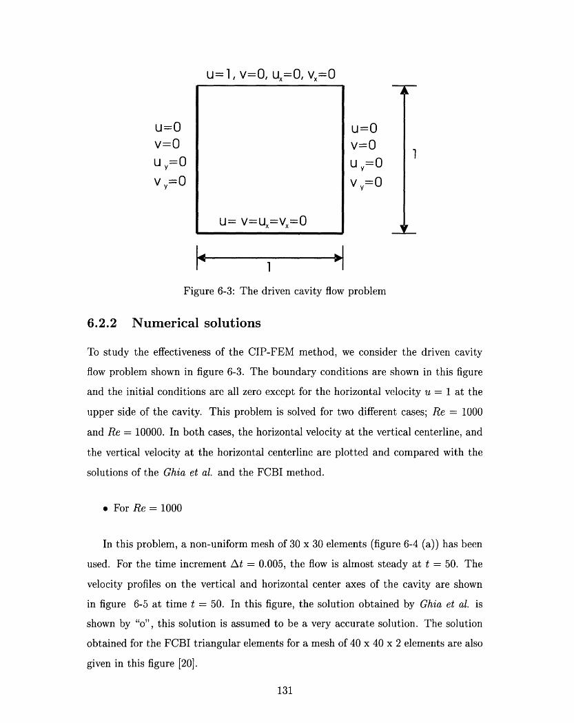
u=1, v=O, u,=O, v,=O

u=Ov=Ouy=OvY=0

A

u=Ov=O

vy=O

v

i

1

Figure 6-3: The driven cavity flow problem

6.2.2 Numerical solutions

To study the effectiveness of the CIP-FEM method, we consider the driven cavity

flow problem shown in figure 6-3. The boundary conditions are shown in this figure

and the initial conditions are all zero except for the horizontal velocity u = 1 at the

upper side of the cavity. This problem is solved for two different cases; Re = 1000

and Re = 10000. In both cases, the horizontal velocity at the vertical centerline, and

the vertical velocity at the horizontal centerline are plotted and compared with the

solutions of the Ghia et al. and the FCBI method.

* For Re = 1000

In this problem, a non-uniform mesh of 30 x 30 elements (figure 6-4 (a)) has been

used. For the time increment At = 0.005, the flow is almost steady at t = 50. The

velocity profiles on the vertical and horizontal center axes of the cavity are shown

in figure 6-5 at time t = 50. In this figure, the solution obtained by Ghia et al. is

shown by "o'', this solution is assumed to be a very accurate solution. The solution

obtained for the FCBI triangular elements for a mesh of 40 x 40 x 2 elements are also

given in this figure [20].

131

u= v=u =vX,=0

As it is clear from figure 6-5, the CIP-FEM method has a higher spatial accuracy

than the FCBI scheme. In addition, the spatial derivatives are more accurate in

the CIP-FEM method since they are considered as nodal variables in the solution.

However, this method requires more computational effort than the FCBI method. For

example, in the CIP-FEM method, the problem is solved in two phases; the advection

phase and the non-advection phase and in each phase after the nodal velocities have

been updated, the nodal spatial derivatives are calculated. In addition, for the non-

advection phase the continuity equation is satisfied by the relaxation method and this

increases the solution time.

It should be noted that although spatial derivatives of velocities are also considered

as nodal variables in the CIP-FEM method, the system of equations for velocities are

solved separately from the system of equations for velocity derivatives (after velocities

are obtained, then the velocity derivatives are updated). In addition, the velocities

in the x and y directions are also uncoupled as seen in equations (6.39) and (6.47).

Therefore, the velocity in each direction is obtained separately.

* For Re = 10000

A non-uniform mesh of 50 x 50 elements (figure 6-4 (b)) with the time increment

At = 0.002 has been used here. After the solution is steady, the velocity profiles on

the vertical and horizontal center axes of the cavity are as shown in figure 6-6. In

this figure, the Ghia et al. and the FCBI solutions are also given. It can be seen that

the CIP-FENI method has higher spatial accuracy than the FCBI scheme (the FCBI

triangular element has been used here [20]).

In order to solve high Reynolds number flows with the traditional finite element

method, we require a very fine mesh. Linking the CIP method to the finite element

method increases the stability of the solution in addition to improving the accuracy

for the velocities and the derivatives.

132

(a)

(b)

Figure 6-4: The non-uniform meshes used for (a) Re = 1000, (b) Re = 10000.

133

IIIIIII II I111111I II I111111I II I11111111 I I11111111 I I11111111 I L11111111 I L11111111 I I11111111 I I,1111 I I I III

-

.__-__

_

I I I I I I II I II I II 1 1 ......

...

-. 1.1.1 11

111111 I I I I II I I II I... Ill ULLULL_ I L I I - I...... IMULL] LLJ l.JL -_ ____ -_ " ' ' I... !HHHH i i 1-41 F - - - I

I I I I I I I I I

I I I I I I ,I I I.. 0:11 ': .:: ':: 0.i~2 ' .:::'i 0. 3 .': . :. : : . ..4: . : : : 0,7 .0 . 01

4 46 '.04 42 - D 0- 0.2

o. ri-- zota o velo iw t0.4 0.6 0.8

Figure 6-5: Velocity profiles for Re = 1000.

134

Ghia et al.CIP -FEM (30x30 elements)FCBI (40x40x2 elements) +

'"4"",.,

.... ' - , . J_+~ +/t .08

04

.2

.1" a

0> -0.2

.0.4

;0.6

. 1

0.

:07

0.6

' 0.8. .0 .4O'sr

., "0.30,2

, 0 : ..

. .

+ /

.~ ,//

.//

?

+

/'

,

. , .3-

l t l _ l l l l l~~~/~"

I

... 1 1, I ... , , :,� �:.� -�. , � . .. .: .. .' ' I . ., 11 .Ir·

·i·:

.. :..,... , =1 I I I. ....... ...................

. :

_

···:·:..' .�·· :;::· :::': ·"'':I; :,;ci::i:;,j·:l., �·;·· ::.: �·�· ·· · . � ::· :·::::-:::�::�::· · · ··�·: . ·.· � : ' . .. ·��· "� ·I�:� :���:·i·..,...···· · · ·...:.. :···...... · · . · ·:··. ::: ;

�

�

. -

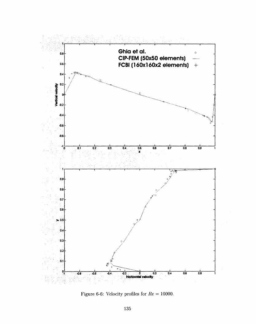
_X G h i et al. -

Ghia et al.CIP-FEM (50:

I I I'

0

x50 elements)FCBI (1 60x1 60x2 elements)

+ /

-,. "I.,..

0.3 :0,4' 0,,-x

I ' ' ! ' ' I ,''+'s

/

/ 1'

f..

/

// ./K~~~~~~~~~. /,~~~~~~, /·/

,

I'-, I I I

.44 . a . ' .. : ' . .0.2.

0.6 0.7 08 0.9

0.4 0.6 0.8

Figure 6-6: Velocity profiles for Re = 10000.

135

.. .: . : :

0.e

0.4

0.2.2

.1;0,II

I

42

.0.4

,.,

,.

-0848z

I

i· ,)x.~

I .i-i

I. 01 . . .0.2

-, -

.' ' '. 9

0.,

,, : 0.

. . ! .S. 0,3- 6

.5

.

0.3

. . 0.2

. . ., -0-10.

' .. I

E

! , : . . i

- . ,,~ I r l r I i....i

I I .. ii �I

.i·

-

-

!I

': 1 _

7.1t .

6.3 Linking the FCBI scheme to the CIP method

The convergence curves shown in figures (4.18)-(4.19) display a small rate of conver-

gence when the FCBI 9-node element is used. In addition, from figures 6-5 and 6-6

we observe that linking the CIP method to the finite element method improves the

accuracy of the solution and velocities are more accurate using the CIP-FEM method.

In order to improve the accuracy of the solution and the rate of the convergence for

the FCBI scheme, the CIP method is here extended for use in the FCBI scheme.

6.3.1 The governing equations

The non-dimensional continuity and momentum equations are written as,

V u=0

all 1 (6.55)t + (u. V)u = -Vp+ V2u

at Re

where u, p and Re are the velocity vector, pressure and the Reynolds number respec-

tively. External force is not considered here.

In the CIP-FCBI method, we need the spatial derivatives of the momentum equa-

tion as follows,

au, V1+ (u. V)U = -(u/. V)u - Vp. ,e V2u

9at Re(6.56)+ (u V)u, = -(un * V)u - Vp, ± V2 u (6.56)atY + (u. V)uy = -(uy V)u - Vpy + Re V 2u y

where the subscripts x and y show the derivative in each direction.

We split the governing equations into an advection phase and a non-advection

phase. The advection phase is solved by the CIP method and the same third order

interpolation functions (6.43)-(6.46) are used. The non-advection phase is solved by

the FCBI scheme.

Note that in the FCBI scheme in the equation (4.1), we consider the Navier-

136

Stokes equations of a two-dimensional incompressible fluid flow at time t when the

solution is at the steady-state. In the CIP-FCBI method, we need to include the time

dependent terms since the velocities and the spatial derivatives of the velocities for

the next time step are obtained by shifting the cubic polynomial in the advection

phase and by updating the velocities and its derivatives in the non-advection phase.

Here in the CIP-FCBI method, we continue the calculation until the solution is at

the steady-state and the velocities, the pressures and the spatial derivatives of the

velocities do not change.

* The advection phase

The governing equations of the advection phase are,

+ (un V)u = At

U x UT + (Un V)U = (6.57)At

flt 8 + (un V)u = At

Considering the advection equation for a potential A,

at + u V = (6.58)

The solution at time "t" is approximated as,

q(xi, t) (xi - J udt, t- dt) (6.59)

where xi denotes the grid point where X is given. The start point x, = xi - f udt

becomes the grid point at the next time step. x, is called the advection distance

and should be calculated along the particle path. However, the exact value of this

distance is difficult to obtain and it is approximated explicitly as,

Ax = xi -x* = u At (6.60)

137

In order for this approximation to be close to the exact value, At must be suffi-

ciently small.

In the CIP method, the potential X is interpolated using the third order shape

functions, and these functions are defined for the system of coordinates -77 within

each sub-element. Since the start point x, is obtained in the x-y coordinate system,

we find the corresponding , and 7, for this point.

The shape function then is defined as,

q(~, ) = ha(, 7)[Ga(, 77) + E(~ ,r)ba] (6.61)a

where ha is the conventional linear shape function, and Ga and Ea are new shape

functions that are second order and linear respectively.

We use the FCBI 9-node elements consist of four 4-node sub-elements shown in

figure 6-7(a) to descretize the fluid domain. For the sub-element shown in figure 6-

7(b), these functions are as follows,

h, = 1 (1 )(1 - 7)

h2= 1 (1 + )(1 - /)1 (6.62)

h3 =I4 (1 (I + +7)h 4=

1

4

E1 = -

1E = -( -)

2 (6.63)E3 = 2 ( + i)

E4 = 2 (-f + q7)

138

4

(a) 9-node elements

4 I

2,

(b) sub-element

2

Figure 6-7: 9-node elements and the 4-node sub-element used in the finite elementdiscretization

1 1G = I(1 - 2)[001 + 1] + (1 - ) [ 0 + 1]2=(+ )2 - 2

1 1 (1 _/2G = (- 12+ )[o02 -( 1 + -2)[o0q2 + 022 2

(-1 + (2)[Oa93 - 03] +

1G4= 2 2

(6.64)

2 (-1 + - 2)[0r/ 3 - 03]

(- 1 + 2 )[071 04 - 04]

Using the CIP-FCBI method, the velocity u and its derivatives are updated for

the time "t" ( i, i, and ifi). These values are then taken to the non-advection phase.

* The non-advection phase

139

1G3 =

2

1

1

The governing equations are as follows,

Un + 1 - 1UA + Vpn+l = V2unAt Re

Un1- X = -(Un V)U _ VPn+1 + V2 u65)At \LX V)U XX Re (6.65)

U+l _ f1xt = -(Un V)un _ VPn+l + -V2UnAt ~ ~ ~y V vy Re y

In order to avoid considering the pressure derivatives px and py as nodal variables

and updating them for each time step in the second and third equations, these terms

are replaced by the velocity terms from the first equation. Then, the second and third

equations are written as,

U t = -(un V)un+ - (- - )

Un+1 - u + 1 (6.66)At = -(Un V) u + a (a )

The non-advection phase is discretized by the FCBI scheme. The finite element

solution is obtained by considering a weak form of these equations and the continuity

equation. Using the Petrov-Galerkin procedure (the test functions do not correspond

to the trial functions), the weak formulation of the problem within the domain Q can

be given as

Find u E U and p E P such that

jw - + VPn+) dQ=iw R V2Un dQ

jq V u dQ = 0

(Un+1 ~ -ii dQ f"_ u1(6.67)jw (ku ) dQ = w (u. V)u + ( At )] d

W Y Y d = w -(u V)u + (dQAt [ n

140

where w C W and q E Q.

For the 4-node sub-element shown in figure 6-7, we use the four corner points to

interpolate the velocity when the pressure is interpolated within each element. The

trial functions in U are defined in each sub-element as,

1u I (1-)(1-7)

hi = 4 (1 + (1 - 7)4

h3 = (1+ )(1+)h 4 =

4

(6.68)

with -1 , r/< 1.

Similarly, the trial functions in the

1

1 -

hp= 11 4

14

4 4

space P are given in each element as,

(1- r)(1- s)

(1 + r)(1 -s)(6.69)

+ r)(1 + s)

(1-r)(1 + s)

with -1 < r, s < 1.

The elements in the space Q are step functions.

at node 2, for example,

hq= {

Referring to Fig. 4.2(a), we have,

1 for (r,s) E [0, 1] x [-1,0]

0 elsewhere(6.70)

Similarly, the weight functions in the space W are also step functions. Considering

the sub-element shown in Fig. 4.2(b), at node 1, for example,

141

hW 1 for (, ) E [-1,0] x [-1,0] (6.71)

10 elsewhere

Then the velocity u and its derivatives and the pressure p in (6.67) are replaced

by

4

u = E hu uii=1

4

u = C h uii=14

Uy - E h ui

i=14

p = S hp pjj=1

The dimensional form of the equations (6.67) is written as

(6.72)

I1n+1 t- W -. At + - pn+) dQ = W 2n dQ

P P

q V. (pu) dQ = 0

--Uw At

W -Y YAt

dQ=iW [-(Un

dQ jI [ (U

a Un+ -· V)u" + ( u

a Un+ _ (· )u + N (ay At

Assembling the first two equations in (6.73) (the momentum and the continuity

equations) for all the control volumes in the body, and using the divergence theorem

we get

142

4Q(6.73)

dQ

dQ

C

(6.74)

KVZVZ Kvy Kvp U1 Rv x

KvYVv KvY K u 2 = RVv

KpVZ Kpvv 0 P O

where ul and u2 contain the nodal velocities in the x and y directions respectively

and p contains the nodal pressures. For a mesh of non-distorted elements, we get

KvXv (i, j) =1

At i 4Qh' dxdy

KvZv, (i, j) = 0

KVx p(i, j) = 5E Wi j p nx dyi P

Kvyvx (i, j) =

KVYv (ij) = Kvv (ij) (6.75)

KvYp(i, j) =

Kpvx (i, j) =

Kpvy (i,j) =

E Wi i

E qQii

E qqii

I hj n dyQ

o h' ny dxQ

Rv (i) = E wniIOQ p

(hjy uln) ny

+ 11 ~ hu dxdy f.1

At I:·i u 3i

Rvy(i) = 5 wfii IQ P

dx + wnii

ILpp

+ It wi hu dxdy U^2

(6.76)

143

- ny dxP

dx + Ei

WQipP

(h~s ) n dy

(hu 2U> 2 (hjU 232> 2n d

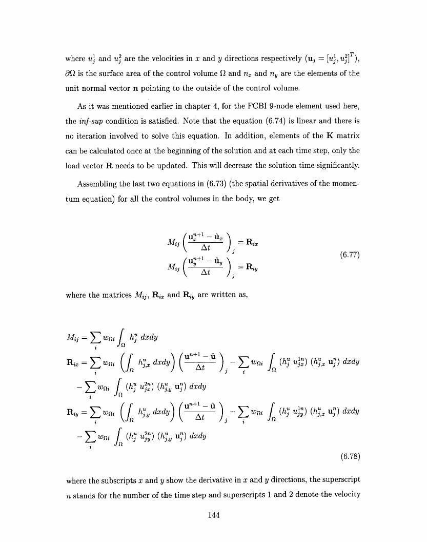
where uj and uj2 are the velocities in x and y directions respectively (uj = [u, u2]T),

OQ is the surface area of the control volume Q and nx and ny are the elements of the

unit normal vector n pointing to the outside of the control volume.

As it was mentioned earlier in chapter 4, for the FCBI 9-node element used here,

the inf-sup condition is satisfied. Note that the equation (6.74) is linear and there is

no iteration involved to solve this equation. In addition, elements of the K matrix

can be calculated once at the beginning of the solution and at each time step, only the

load vector R needs to be updated. This will decrease the solution time significantly.

Assembling the last two equations in (6.73) (the spatial derivatives of the momen-

tum equation) for all the control volumes in the body, we get

(6.77)

Mi+ - Al ) = Rx

Mij SAt j iy

M~~j At j

where the matrices Mij, Rix and Riy are written as,

Mij = E wS-i j h dxdyi

iRi = WsZwi (f | hx dxdy)( UnWAt -Q

i J iWi w u (b y ,j) (h;y u?) dxdyRiy = E W~si (IQ h~v dxd8) (~~At WQ

- EWQ i (hu u2n ) ( u) dxdy2~~~~j ,

j (hju un) (hj un) dxdy

(hui uln) (hUx un) dxdy

(6.78)

where the subscripts x and y show the derivative in x and y directions, the superscript

n stands for the number of the time step and superscripts 1 and 2 denote the velocity

144

in x and y directions respectively. For a non-distorted mesh, the Mij matrix is the

same for all the elements and therefore the assemblage will be easy.

In the non-advection phase, first the velocity u n+1 and the pressure pn+l are

obtained from the equation (6.74), the velocity un +1 is then used in (6.77) to obtain

u n+l and u +1 . The calculations for one time step are complete now and for the next

time step, we take the values un+1, pn+l, un+1 and u +1 to the advection phase and

we repeat the calculations for the new time step.

The solution process is given in table 6.3.1.

Table 6.3.1 Solution process in the CIP-FCBI method for incompressible flows

(1) Set initial conditions un and the spatial derivatives un and for all the

nodal points (the superscript n denotes the solution at time t - At).

(2) From the advection phase use the CIP solver to obtain fi and the spatial

derivatives fix and fly for all the nodal points using equations (6.61)- (6.64).

(3) From the non-advection phase, use the FCBI scheme to obtain Un+l and

pn+l from the equation (6.74).

(4) From the non-advection phase, obtain the spatial derivatives u +1 and u + 1

from the equation (6.77).

(5) Repeat (2) to (5) for the next time step.

6.3.2 Numerical solutions

To study the effectiveness of the CIP-FCBI method, we again consider the driven

cavity flow problem shown in figure 6-3. The boundary conditions are shown in this

figure and the initial conditions are all zero except for the horizontal velocity u = 1 at

the upper side of the cavity. This problem is solved for two different cases; Re = 1000

and Re = 10000. In both cases, the horizontal velocity at the vertical centerline, and

the vertical velocity at the horizontal centerline are plotted and compared with the

solutions of the Ghia et al., the CIP-FEM method and the FCBI method.

* For Re = 1000

145

In this problem, a non-uniform mesh of 32 x 32 sub-elements (16 x 16 elements)

(figure 6-8 (a)) has been used. For the time increment At = 0.005, the flow is almost

steady at t = 35. The velocity profiles on the vertical and horizontal center axes of

the cavity are shown in figure 6-9 at time t = 35. In this figure, the solution obtained

by Ghia et al. is shown by "o", this solution is assumed to be the exact solution.

The solution obtained for the FCBI triangular elements for a mesh of 40 x 40 x 2

elements [20], and the solution obtained for the CIP-FEM method for a mesh of 30 x

30 elements (figure 6-4 (a)) are also given in this figure.

As it is clear from figure 6-9, the CIP-FCBI method has a higher spatial accuracy

than the FCBI scheme. In addition, the spatial derivatives are more accurate in

the CIP-FCBI method since they are considered as nodal variables in the solution.

However, this method requires more computational effort than the FCBI method. For

example, in the CIP-FCBI method, the problem is solved in two phases; the advection

phase and the non-advection phase and in each phase after the nodal velocities have

been updated, the nodal spatial derivatives are calculated. The velocities are slightly

more accurate using the CIP-FEM method. However, the CIP-FEM method requires

more computational effort than the CIP-FCBI method since for the non-advection

phase, the continuity equation is satisfied by the relaxation method and this increases

the solution time.

It should be noted that although spatial derivatives of velocities are also considered

as nodal variables in the CIP-FCBI method, the system of equations for velocities are

solved separately from the system of equations for velocity derivatives (after velocities

are obtained, then the velocity derivatives are updated).

* For Re = 10000

The non-uniform mesh of 64 x 64 sub-elements (32 x 32 elements) shown in fig-

ure 6-8 (b) with the time increment At = 0.002 has been used here. After the solution

is steady, the velocity profiles on the vertical and horizontal center axes of the cavity

are as shown in figure 6-10. In this figure, the Ghia et al., the CIP-FEM, and the

FCBI solutions are also given. It can be seen that the CIP-FCBI method has higher

146

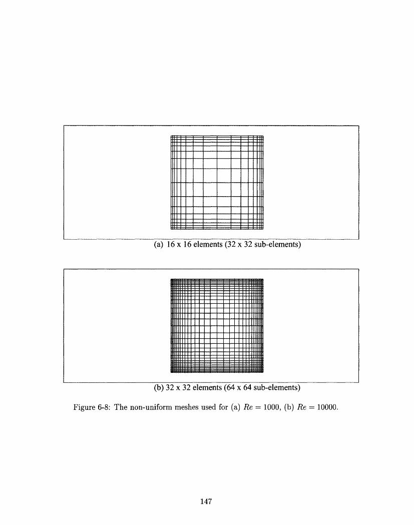
(a) 16 x 16 elements (32 x 32 sub-elements)

. |". S ,L__

[tl. .,__ I I 1..1 I WW _I I I I _ _ 1 .1111

(b) 32 x 32 elements (64 x 64 sub-elements)

Figure 6-8: The non-uniform meshes used for (a) Re = 1000, (b) Re = 10000.

147

HW-C+ ---- - -- L-L H·

HH+1 - - II!11·

Htl t - - -- +--trm

H+ - -* - llm

I

I

I

0.3

0. 2

0.1

kP O#0.,0

.I.

.o3

.0.4

0 . . ' . : . .: 0. ;. 2 0 . .'

.. .. ... ~~~~~~~~~~~ .. .. .. . .. :'. " . ''" '' ' /, .

1~~~~~'''';:"'f '"

: 0.5 0.6 0,7:0 ' . . .0~ :. "'.:..0 ;?

. . .

08 0.9 1

i- rlzc m~i VJOCRYrt

Figure 6-9: Velocity profiles for Re = 1000.

148

>0ooO - lr-irrr T·.r~-t- ,,.~,~.~.:~~~ ~ :: :

/ -.rs '\f XA~~~~~~~~~~~~~~~~~~~~.~~~~~~~~~~~~~~~~~~~~~~~~~~~~~~~~~~~~~~~~~~~~~~~-....,

I a.~~~~~~~~~~~~~~~~~~~~~~~~~~~~~~~~~

X,,!/"--

N N. ~~~~/

Ghia et al. o ' CIP-FCBI (16x 6 elements) " ,CIP-FEM (30x30 elements) * aidFCBI (40x40x2 elements) + ' ?

~I I I I I I.~ I ~A II

"I

If

. .. .

spatial accuracy than the FCBI scheme (the FCBI triangular element has been used

here [20]). However, the velocities are slightly more accurate using the CIP-FEM

method.

* Concluding remarks on the numerical results

Of course we can only draw partial conclusions from these preliminary numerical

results since, in particular, other fluid problems need to be solved for comprehensive-

ness.

From these numerical results, the CIP-FEM and the CIP-FCBI methods appear

to predict the solution more accurately than the traditional finite element method and

the FCBI scheme. In order to solve high Reynolds number flows with the traditional

finite element method, we require a very fine mesh. Linking the CIP method to the

finite element method increases the stability of the solution in addition to improving

the accuracy for the velocities and the spatial derivatives. In order to obtain accurate

solutions for high Reynolds number flows, we require a finer mesh for the FCBI

method than for the CIP-FCBI method. Linking the CIP method to the FCBI scheme

improves the accuracy for the velocities and the derivatives. In addition, when the

flow is not at the steady state and the time dependent terms need to be included in

the Navier-Stokes equations, or in the problems when the derivatives of the velocities

need to be obtained to high accuracy, the CIP-FCBI method is more convenient

than the FCBI method. However, both the CIP-FEM method and the CIP-FCBI

methods require more computational effort than the finite element method and the

FCBI scheme (and it takes longer for these methods to stabilize the flow) since the

advection phase is solved by the CIP method. In addition, in the CIP-FEM method,

the continuity equation is satisfied by the relaxation method and this increases the

solution time.

149

I i I I I I

)t al. 0

/

I) K I

\m *t+

I I I I I I I I I

CIP-FCBI (32x32 elements)CIP-FEM (50x50 elements)FCBI (1 60x1l 60x2 elements)

0.3 0A. . ..-0.6 x1

*

0.8 0.7 0s 0s

.Hoizronal iocy

Figure 6-10: Velocity profiles for Re = 10000.

150

Ghia e

0.4

0.2

00

. 1

goB

-0.4

-0.6

1

0.9

0,7

. . oil~l·. ... ...

0.6

>, 0.5

.4

0.3

0.2

:: .01

,5

/

/,

/

/

O /

.0

®/ "IfA

.Fun I ~ ~ ~ ~ ~ ~ ~ ~ ~ ~ ~ ~ ~ ~ ~ ~~~~~~~~~~~~~~~~~~~~~~~~~~~ I m f . . . . _ _ _.

,, _............_ ----·I� ---

,L f I.... - -7- ~ -·-- :- -

:: I )·� ·i\�·)� ·I �··. �.... .i·i.: · ·i� � i·l ·i·i···r·%···: ·· ··X ·· ·· ·., ···· : UMi . I I I

I

t

6

0

-

-

-

-

a

Chapter 7

Conclusions

The Navier-Stokes equations are widely used for the analysis of incompressible laminar

flows. If the Reynolds number is increased to certain values, oscillations appear

in the finite element solution of the Navier-Stokes equations. In order to solve for

high Reynolds number flows and avoid the oscillations, one technique is to introduce

artificial upwinding into the equations to stabilize the convective term, ideally without

degrading the accuracy of the solution: e.g. the streamline upwind/Petrov-Galerkin

(SUPG) method, the Galerkin/least-squares (GLS) method, the Cubic Interpolated

Pseudo/Propagation (CIP) method and use of the bubble functions.

The analysis of fluid flows with structural interactions has captured much attention

during the recent years. Such analysis is performed considering the solution of the

Navier-Stokes fluid flows fully coupled to the non-linear structural response. However,

a fully coupled fluid flow structural interaction analysis can be computationally very

expensive. The cost of the solution is, roughly, proportional to the number of nodes

or grid points used to discretize the fluid and the structure. In order for interaction

effects to be significant, the structure is usually thin and can be represented as a shell,

hence not too many grid points are required. The large number of grid points and

consequently, number of equations in fluid flow structural interaction problems (FSI)

is due to the representation of the fluid domain. For high Reynolds number fluid

flows, to have a stable solution, more grid points are required. In order to decrease

the number of grid points in the fluids (using a coarser mesh) and still have a stable

151

solution, the flow-condition-based interpolation (FCBI) procedure was introduced.

The FCBI is a hybrid of the finite element and the finite volume methods and

introduces some upwinding into the laminar Navier-Stokes equations by using the ex-

act solution of the advection-diffusion equation in the trial functions in the advection

term. The test functions for both the continuity and the momentum equations are

step functions and the governing equations are written over control volumes. Hence,

the mass and momentum conservations are satisfied locally. Ideally any numerical

solution for fluids should yield stable solutions for low and high Reynolds number

flows with reasonable accuracy. Of course, when fine meshes are used, more details

of the flow are captured and the level of accuracy is higher. Ideally, we want our

numerical scheme to yield still stable solutions with reasonable accuracy when coarse

meshes are used. In particular, this will decrease the required number of grid points

and elements in the fluid phase in the fluid-structure interaction problems.

The previous works on the FCBI procedure include the development of a 4-node

element and a 9-node element consisting of four 4-node sub-elements. In this thesis,

the stability, the accuracy and the rate of convergence of the already published FCBI

schemes was studied. From the numerical results, the FCBI 9-node elements (consist

of four 4-node sub-elements) appear to be stable for high Reynolds numbers although

no upwind parameter is used, and predict the solution reasonably accurate. Of course,

in order for the solution errors to be small, the mesh needs to be refined. However,

the convergence curves used for the u - Uh IlL2 , 11 U - Uh IH1 and p - Ph HiL2

norms, display a small rate of convergence when the FCBI 9-node elements are used.

In order to ensure that using the coarse meshes to represent the fluid yields an

accurate enough structural response, the solution errors need to be controlled and

measured. The "goal-oriented error estimation" might be applied to assess the error in

the quantities of interest in the structure. In fluid flow structural interaction analysis,

it is ideal to use an FCBI solution scheme in rather coarse meshes together with

"goal-oriented error estimation" to control the error of the solution in the structural

response.

From the numerical results, it became clear that the earlier published FCBI 9-

152

node elements (consist of four 4-node sub-elements) are more stable than the Galerkin

9-node elements. However, the Galerkin 9-node elements give more accurate solutions

with a higher rate of convergence. Hence, a new FCBI 9-node element was proposed

that obtains more accurate solutions than the earlier proposed FCBI elements. The

new 9-node element does not obtain the solution as accurate as the Galerkin 9-node

elements but the solution is stable for much higher Reynolds numbers (than the

Galerkin 9-node elements), and accurate enough to be used to find the structural

responses.

The Cubic-Interpolated Pseudo-particle (CIP) method is a very stable finite dif-

ference technique that can solve generalized hyperbolic equations by the 3rd order

of accuracy in space. In this method, a cubic polynomial is used to interpolate the

spatial profile of the value and its spatial derivative. The spatial derivative itself is

a free parameter and satisfies the master equation for the derivative. After the value

and its spatial derivative are found, the same values for the next time step are simply

calculated by shifting the cubic polynomial. For nonlinear problems, the CIP scheme

splits the hyperbolic equation into two phases; the non-advection phase and the ad-

vection phase. In each time step, after the non-advection phase is solved by the finite

difference method, the CIP method is applied to the advection phase.

The CIP method was originally proposed for the finite difference method; both

the convection phase and the non-convection phase are solved using the finite differ-

ence method. However in some problems, satisfying the boundary conditions for the

incompressible Navier-Stokes equations is easier using the finite element methods. In

addition, in problems for which the domain is complicated and mesh grading is re-

quired, the finite difference methods are not as flexible as the finite element methods.

In this thesis, the CIP method was extended for use in the finite element method

(CIP-FEM) and the FCBI scheme (CIP-FCBI). The finite element shape functions

for the third order interpolation were defined by the product of the linear shape

function and a new second order shape function. These functions were used to solve

the two-dimensional incompressible Navier-Stokes equations.

From the numerical results, the CIP-FEM and the CIP-FCBI methods appear to

153

predict the solution more accurate than the traditional finite element method and the

FCBI scheme. In order to solve high Reynolds number flows with the traditional finite

element method, we require a very fine mesh. Linking the CIP method to the finite

element method increases the stability of the solution in addition to improving the

accuracy for the velocities and the derivatives. In order to obtain accurate solutions

for high Reynolds number flows, we require a finer mesh for the FCBI method than

for the CIP-.FCBI method. Linking the CIP method to the FCBI scheme improves

the accuracy for the velocities and the derivatives. In addition, when the flow is not

at the steady state and the time dependent terms need to be included in the Navier-

Stokes equations, or in the problems when the derivatives of the velocities need to be

obtained to high accuracy, the CIP-FCBI method is more convenient than the FCBI

method. However, both the CIP-FEM method and the CIP-FCBI methods require

more computational effort than the finite element method and the FCBI scheme (and

it takes longer for these methods to stabilize the flow) since the advection phase is

solved by the CIP method. In addition, in the CIP-FEM method, the continuity

equation is satisfied by the relaxation method and this increases the solution time.

This work represents only a first step in liking the FCBI scheme to the CIP

method, more work could be done to improve the accuracy of the solution in the

CIP-FCBI method. In addition, to study the accuracy and convergence of the FCBI

9-node elements, we considered the L2 and H1 norms of the velocities and L2 norm of

the pressure, better norms could be found to measure the errors in the FCBI scheme.

154

Appendix A

Consistency of the CIP scheme

The difference scheme Efn = 0 is consistent with the differential equation L2f = 0 if

for all grid points j and time steps n

(tfn)j - (f) -+ 0 (A.1)

when Ax, zt -+ 0.

In this appendix, we prove the consistency of the CIP scheme for the one-dimensional

non-linear hyperbolic equation

Of Of Oua+u- =G=g-fa (A.2)at O x ax

As it was explained in chapter 6, f' should satisfy the spatial derivative of the

master equation (A.2) as

af' Of' _ ' u (A.3)+ U G '- I (A.3)at aU- - x

In order to solve (A.2) and (A.3), the CIP scheme splits the problem into two

phases; the non-advection phase and the advection phase. The non-advection phase

is solved by a finite difference scheme while the advection phase is solved by the CIP

solver.

* Non-advection phase

155

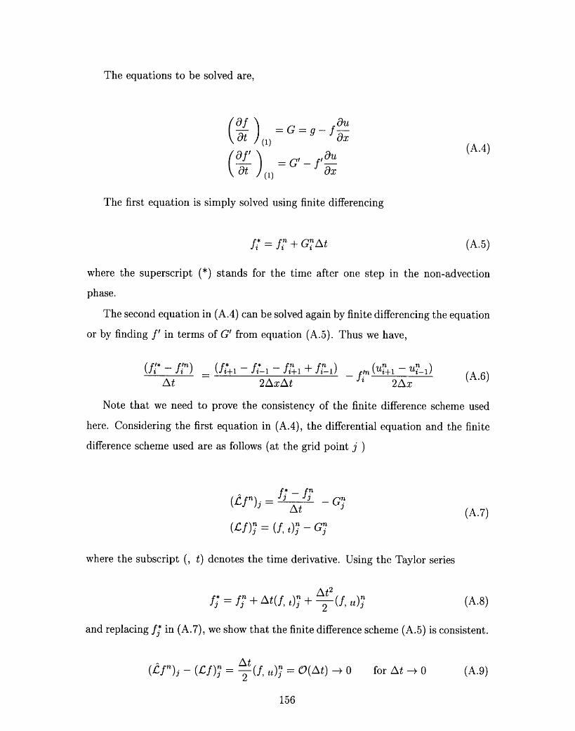
The equations to be solved are,

af

Oaf

at

=u= G = g f

ax) (1)

(1)

The first equation is simply solved using finite differencing

fi* = f + GiAt (A.5)

where the superscript (*) stands for the time after one step in the non-advection

phase.

The second equation in (A.4) can be solved again by finite differencing the equation

or by finding f' in terms of G' from equation (A.5). Thus we have,

(fi* - fl) (f+ 1 -At

i- -fin+xt + 2Axz/\t

_ fn (un+l - Un1)2Ax

Note that we need to prove the consistency of the finite difference scheme used

here. Considering the first equation in (A.4), the differential equation and the finite

difference scheme used are as follows (at the grid point j )

(2f) - _ f -f n(Atf) = (A.7)

(cf f) = (f, t)n _ Gn

where the subscript (, t) denotes the time derivative. Using the Taylor series

n t2f; = f + At(f, )j + (f, tt)n (A.8)

and replacing fj in (A.7), we show that the finite difference scheme (A.5) is consistent.

n 2t(f, )n = O(At) - o for At -- 0

156

(A.4)

(A.6)

(A.9)

= G' - f'dir;

Now, we consider the second equation in (A.4)

at = G'- f Ou19X

(A.10)) (1)

where the differential equation and the finite difference scheme at the grid point j are

as follows

f* - f n(Lfn)j

fj+l- f-1- fj l + f j-12AxAt + fn j+2 - UY-12Ax

(Cf)n = (f t), - (G, x)n + (f, x)n(U, x)y

Using equation (A.5), we can use relations

- f +lAt Gj +l

f*l- f- nJAt- 1 1 = GnAt -1

to obtain

(~lf')j: fj1* - fin G - Gf n = At 2Ax

Using the Taylor series

fI* = f n + At (f' t) +2 (fA tt)Ax2

G+l = G + a(G, )+ 2 (G

Ax2

Gjn_ = G - Ax(G, x)j + 2 (G

Ax2

Uj+1 i-ui± X(ux)j 2 (U, x

j_ 1 = - Ax(u, X)?Ax2

+2

n Ax3

, x)j + 6 (G, xxx)n

Ax3

Ax:x? + 6 (u,

Ax3

and substituting them in equation (A.13), we prove the consistency of the finite

157

(A.11)

(A.12)

n uj 1 - U

2Ax(A.13)

(A.14)

difference method used.

(f)j(f)_ At2 (f (G, xx) +(fx) 6 (u, zxa)? = O(At, Ax 2) 0

(A.15)

for At, Ax - 0.

After f* and f'* are found, they will be taken to the advection phase.

* Advection phase

The equations to be solved are as follows,

af N af(af + =o (A.16)at (2) Ox

The CIP solver is applied to the advection phase and the interpolated profile

is determined from equations (6.7) and (6.8 ) using f* and f'* on the right-hand

side. Since the CIP solver uses the analytical solution, there is no need to prove the

consistency of the advection phase.

Note that adding equations (A.4) and (A.16) give equations (A.2) and (A.3) since,

Of _ af a ) af)

aft f (A.+ 1Of7)at at (1) at (2)

Solving these equations in two phases is consistent since the values at the end of

the non-advection phase (f* and f'*) are taken to the advection phase as the initial

values.

158

In this appendix, we proved the consistency of the CIP scheme for the one-

dimensional non-linear equation. For more general cases, a similar procedure is fol-

lowed.

159

160

Appendix B

Stability of the CIP scheme

Consider the difference scheme

fn+l = S n (B.1)

where S is the matrix relating the solution at time t (fP) to the solution at time t +At

(fn+l), and

f= [fl f2 *.. (B.2)

This difference scheme is stable if there exists CT such that

Ilfnll = IISnf11 < CTl1f11 (B.3)

for all f0; and n, At such that 0 < nat < T. Note that the superscript n stands for

the time except in Sn that denotes the power.

The stability analysis of the usual finite difference method is generally formulated

using the discrete Fourier transformation (the von Neumann stability criterion). Since

the CIP scheme involves spatial derivatives, the von Neumann stability analysis is

applied with some modifications. In this appendix, we prove the stability of the CIP

scheme for the linear equation when the velocity is constant (this appendix presents

the stability in the advection phase). For more general cases, a similar procedure is

161

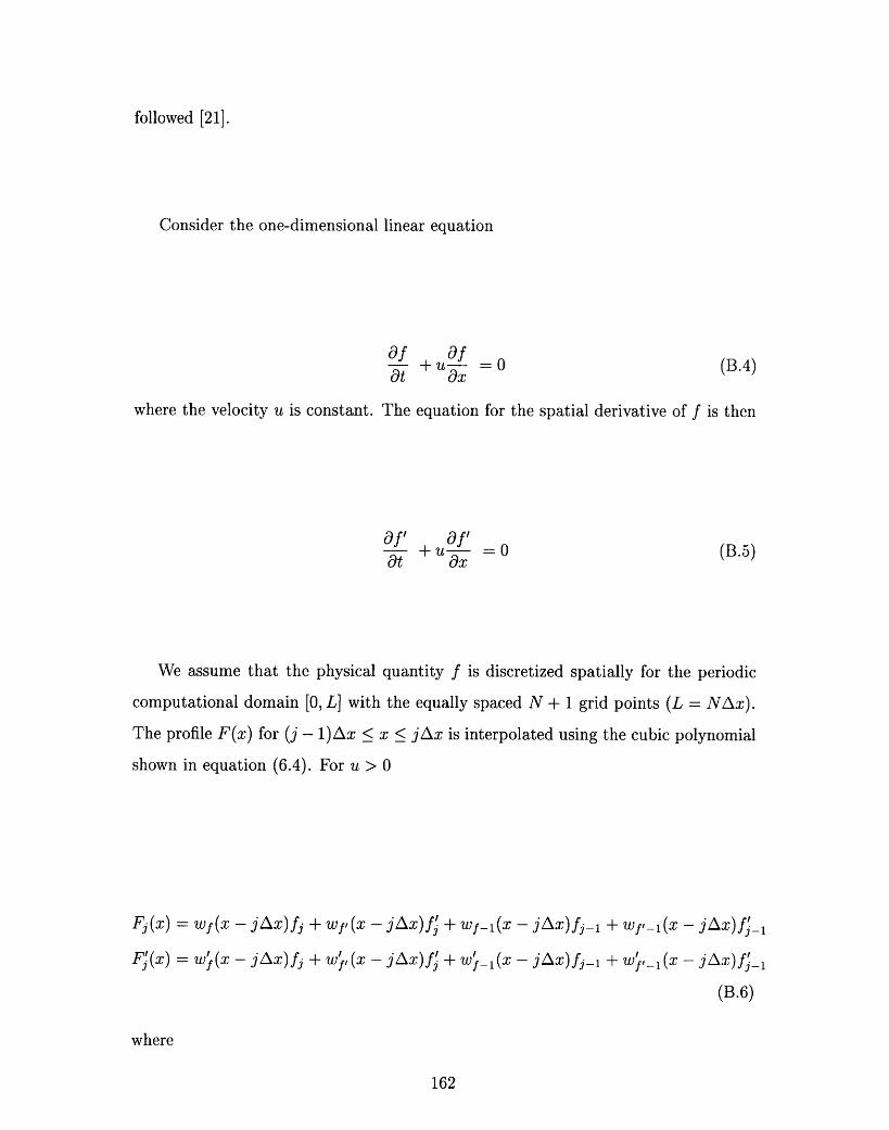
followed [21].

Consider the one-dimensional linear equation

Of Of+ua =O (B.4)at + u=0

where the velocity u is constant. The equation for the spatial derivative of f is then

Of' Of'+ uaf =0 (B.5)at Ox

We assume that the physical quantity f is discretized spatially for the periodic

computational domain [0, L] with the equally spaced N + 1 grid points (L = NAx).

The profile F(x) for (j - 1)Ax < x < jAx is interpolated using the cubic polynomial

shown in equation (6.4). For u > 0

Fj(x) = f(X - jAx)fj + Wf,(X - jAx)fj + wf-l(x - jAx)fjl + wf'-1(x - jAx)fj_

Fj'(x) -= w((x - jAx)fj + WI (x - jx)f + w(x(x - jAx)f-l + W_ (x- jAx)fj

(B.6)

where

162

Wf(X) = 1 - 3X2

Ax 2

2x2

w(X)=X-+ Yx,:12

Wf-l(X) = AX 2

x2

Wfl(x) = A -Ax6x

W (x) = - 2 -

4xW, () = 1 A

f-l(x) =6x

Ax 2

6x2

+ A-X

I 2x 3x 2

Wfl ( x) = Ax Ax2Ax: z

Since the function Fj(x) is continuous and periodic, Fourier coefficients for wave

number k = 2nL (n = 0, ±1, 2, ..- ) are written as

N

F(k)= Ej=lN

=Ej=1

N 0O

Fj(x) eikx dx = E /j=1

eikjAx

Fj(x + jAx) eik(x+j ax) dx

= Wf(k)F(k) + Wfr (k)F'(k)

= [ f(k) Wf (k) ] [1 0 F'(k)f 0~~O 1 P F(k)I

(B.8)

where the notation i is /ZT and

163

2X3

x 3

AX2

2x3

AX3

X3

Ax2

6x2

Ax 3

3x2

+Ax2

(B.7)

(wf(z)fj + wfl(x)f, + wfl(x)fj- + wf (x)fjj + ) eikx dx

-

-IA

Wf (k) = [f (k) + Wfl (k) eikAx]

WfI (k) = [ft (k) + f, _l(k) eikAx]

N

F(k) = Ej=1

eikjzx f

N

F'(k) = E (j=1

Wf(k) =

-Ax-Ax

Wf_l (k) =IAx

wftl(k) = Ax

IikjAx ffj(B.9)

f(X) eikx dx

If?(x) eikx dx

Wf-l(x) eikx dx

wfI-l () eikx dx

Since F(k) represents the discrete Fourier coefficients for the continuous function

f(x), it satisfies

F(k+ r ) = F(k)L

F(k) = F*(-k)27r

forL

(B.10)< < kN- L

F(O) = F*(O)

where the superscript (*) denotes the complex conjugate.

Applying the CIP solver, f+l and f+l are updated as

fin+ = F(xi - u/t)fin+l dF(xi - uAt)

dx

(B.11)

or

164

f3+l = ffj7 + Cffjn + Cflfjn 1 + cCf-lf-1i

fn+l = Cf n + Cfn + C n In,fj -cCf + fj1 + cillj_ 1 +CZ,_1

where

Cf = (1 - 3C2 + 2c 3)

CfI = (-c + 2C2 - C3 )Ax

Cfl- = (3C2 - 2C3)

Cfr-l = (C2 - c3)Ax

6c - 6c2

cf = Ax

c, = (1 - 4c + 3c2)-6c + 6c2

Cf-1 A

cIf,l = (-2c + 3c2)

and c = uAt/Ax (the Courant-Friedrich-Lewy (CFL) number).

The Fourier transform of f after one time step is as follows

165

(B.12)

(B.13)

Pn+l(k) =N

E eik j A x [WVf(k)fjn+' + Wf(k)fj n+l]

j=1

IV

eikjAx ([Wf(k) (cf + eikAxcfl) + Ti- Wf(k)(c' + eikc fl fj:=1

+ [Wf(k)(cf, + eixcf'_l) , ()( + Wf(k) ( eikx,_)] )f +e j_> 1fn(B.14)

= [f(k)Cf + Wf (k)Cf] Fn(k) + [Wf(k)Cf, + Wf,(k)Cf,] Fn(k)

[ Wf(k) Wf(k) ] S(k)[

F'(k)Fn (k)

where

(B.15)

and

Cf = (f + eikAcf _l)

Cf = (Cf + eikAx cf _1 )

Cf, = (Cf, + eikAx Cfl)(B.16)

C; = (Cf, + eik/xcf,_l)

If we repeat applying the above procedure and we use equation (B.8), we obtain

[

and

Fn(k) S�( [FO(k)F'n(k) F'0 (k)

]

(B.17)

166

S(k) = Cf Cf

F (k) = [ Wf(k) WfV,(k) ] S (k) F(k) ] (B.18)F' 0 (k)

For the stability of the CIP scheme, the growth of the errors should be bounded;

the absolute values of all the eigenvalues of the S(k) should be less than unity. The

matrix S(k) is periodic over the domain [0, 27r] of the independent variable (kAx)

and S(k) =,S*(-k). This matrix has eigenvalues

, 2 =3eikAx 2 + 1 _ eikAxc3 C3 _ eikAxc- 2C [(- 1)2 c2 (c2 + e2 i k x C2

- 2 eikAz c2 - 4 e2ikAx c + 2eikAx c + 2c + 10 eikax - 2 + e2ikAx)]05

(B.19)

The absolute values of A1 and A2 are less than unity for 0 < kAx < r and c < 1.

Note that in this appendix, we proved the stability of the CIP scheme for the linear

equation when the velocity is constant. For more general cases, a similar procedure

is followed.

167