Development of a Flexible Pavement Database for Local ...dot.state.nm.us/content/dam/nmdot/Research/MultimediaPresentationM...NMDOT Design Method AASHTO 1972 for Pavement Design with

Development of a Flexible Pavement Database for Local

Calibration of MEPDG

Outline

• This multimedia presentation consist of 3 parts:▫ Development of the MEDPG Database▫ MEPDG Sensitivity Studies▫ Local Calibration of MEPDG

2

Introduction to MEDPG Project

3

NMDOT Design Method

AASHTO 1972 for Pavement Design with Probabilistic Approach

AASHTO 1993 for Check

▫ Based on AASHTO Road Tests in the 1960’s▫ Not Able to Predict Pavement Performance▫ Traffic Load Spectra, Climate are not Considered▫ Different Superpave mixes, Binders are not considered▫ Structural Number is considered only▫ Typically Conservative

4

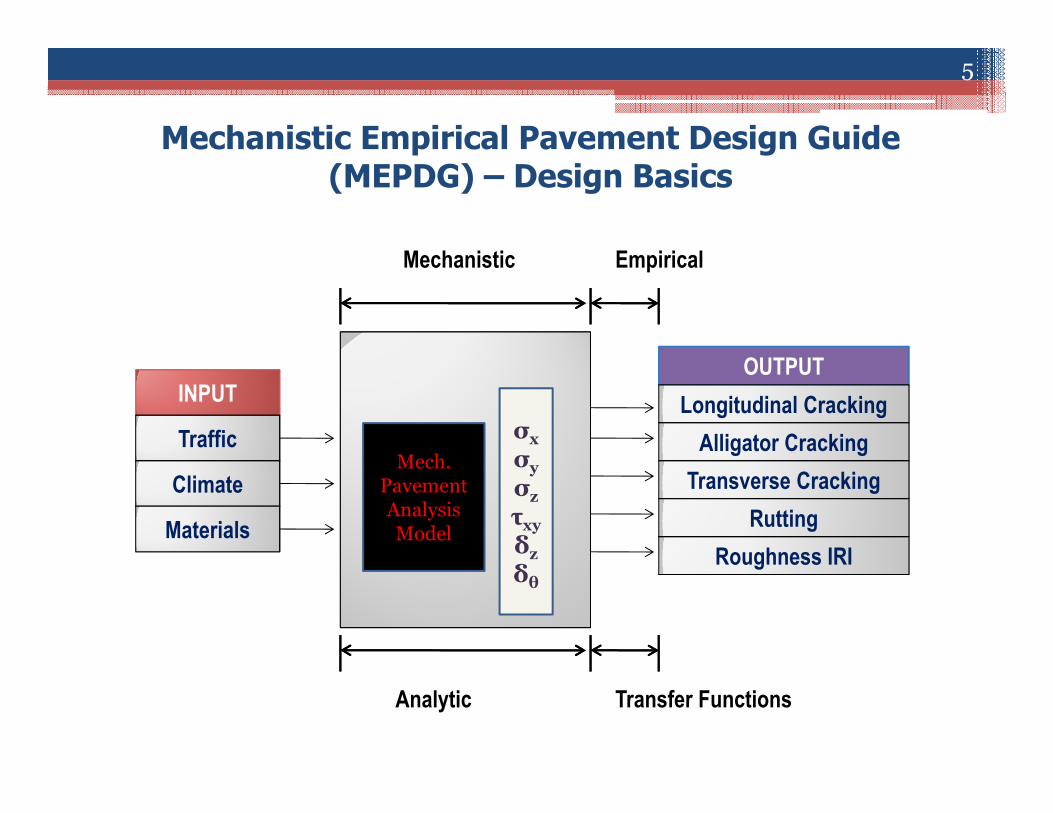
Mechanistic Empirical Pavement Design Guide (MEPDG) – Design Basics

Mechanistic Empirical

Transfer FunctionsAnalytic

Mech.Pavement Analysis Model

σxσyσzτxyδzδθ

INPUT

Traffic

Climate

Materials

OUTPUTLongitudinal Cracking

Roughness IRI

Alligator CrackingTransverse Cracking

Rutting

5

Benefits of MEPDG

Effects of Differences in Climatic Conditions are Considered

Better Modeling of Pavement Materials

Incorporation of the Effects of Vehicles, tire pressures, etc.

Development of Better Pavement Diagnostic Techniques

Consideration of Seasonal and Aging Effects on Materials

6

AASHTO 1993 vs. MEPDG

Parameter AASHTO 1993 MEPDGTraffic ESAL (Equivalent Single Axle

Load), Truck Equivalent FactorAxle Load Spectra, Vehicle Class Distribution, Traffic Growth Factor, Truck speed

Materials Layer Coefficient, Resilient Modulus

Dynamic Modulus (E*),Resilient Modulus (Mr), Complex Modulus (G*)

Climate Seasonal Adjustments, Drainage Coefficients

Thermal properties, Wind Speed, Air Temperature, Depth to Water Table

Performance Design Life Rut, IRI, Different Type of Cracking

Outputs Structural Number or Pavement Thickness

Distress Over Time

7

Example of MEPDG Traffic Input

0

10

20

30

40

50

Cla

ss 4

Cla

ss 5

Cla

ss 6

Cla

ss 7

Cla

ss 8

Cla

ss 9

Cla

ss 1

0

Cla

ss 1

1

Cla

ss 1

2

Cla

ss 1

3

AA

DTT

Dis

tribu

tion

By

Veh

icle

Cla

ss (%

)

I 25I 40US 550 (NM 44)

Vehicle Class Distribution

Year Month Hour Axle Type

Load group0-2 2-4 ….. x-y

Single

Tandem

Tridem

Quad

Table: Axle Load Spectra

Axle SpacingTire Pressure

Wheel Base

General Traffic Inputs• Gear/Axle Configuration• Axle/Tire Spacing• Tire Pressure• Traffic Wander

8

Example of MEPDG Climatic Input

Create Virtual Weather Station byAveraging Surrounding Sites

Identify Weather Station

Choose from 800 sites

Insert Depth for Water Table

9

PG 5

8-28

PG 6

4-28

PG 7

0-22

PG 7

6-22

PG 8

2-22

AC

-20

0

0.1

0.2

0.3

0.4

0.5

0.6

0.7

Rutting Depth (in)

AC RutTotal Rut

PG 5

8-28

PG 6

4-28

PG 7

0-22

PG 7

6-22

PG 8

2-22 AC

-20

100

104

108

112

116

120

Terminal IRI

(in/mile)

PG 5

8-28

PG 6

4-28

PG 7

0-22

PG 7

6-22

PG 8

2-22

AC

-20

0

0.5

1

1.5

2

2.5

3

3.5

4

Long. Cracking

(ft/mi)

PG 5

8-28

PG 6

4-28

PG 7

0-22

PG 7

6-22

PG 8

2-22

AC

-20

0

0.1

0.2

0.3

0.4

Alligator Cracking

(%)

Variable Performance Grade

Influence of PG Grade on I-25 Using MEPDG

**AC-20 is Used for Existing Design

10

Local Calibration of MEPDG

Why Need Local Calibration MEPDG was Developed Using Pavement Data from LTPP Sections of all over USA

Among them NM has Only Two Test Sections (I10 & I25 District 1)

Maximum Benefits from MEPDG - LOCAL CALIBRATION

What is Local Calibration Minimizing the Difference Between the MEPDG Predicted Output Values and the

Field Observed Distresses of New Mexico’s Flexible Pavements

How to Do Local Calibration Adjusting the Distress Model Coefficients in MEPDG

Testing Localized Materials

Perform test section evaluations of stress/strain

11

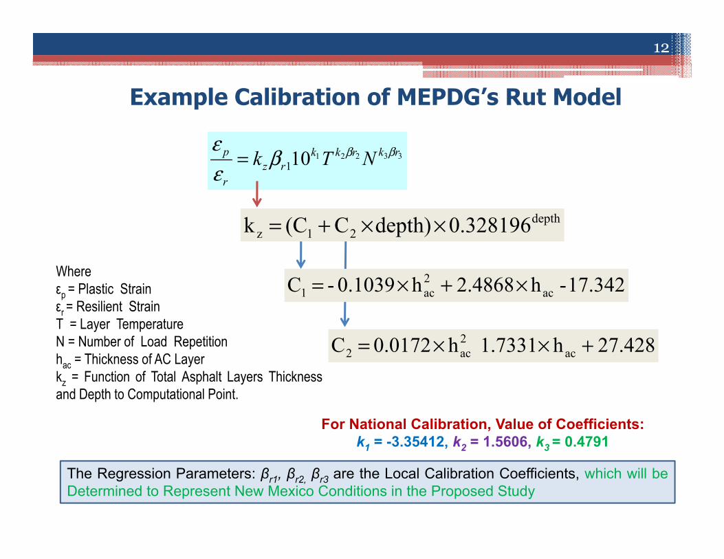
Example Calibration of MEPDG’s Rut Model

Whereεp = Plastic Strainεr = Resilient StrainT = Layer TemperatureN = Number of Load Repetitionhac = Thickness of AC Layerkz = Function of Total Asphalt Layers Thicknessand Depth to Computational Point.

For National Calibration, Value of Coefficients: k1 = -3.35412, k2 = 1.5606, k3 = 0.4791

33221101rkrkk

rzr

p NTk βββεε

=

depth21z 0.328196depth)C(C k ××+=

27.428 h 1.7331 h 0.0172 C ac2ac2 +××=

17.342- h2.4868 h0.1039- C ac2ac1 ×+×=

The Regression Parameters: βr1, βr2, βr3 are the Local Calibration Coefficients, which will beDetermined to Represent New Mexico Conditions in the Proposed Study

12

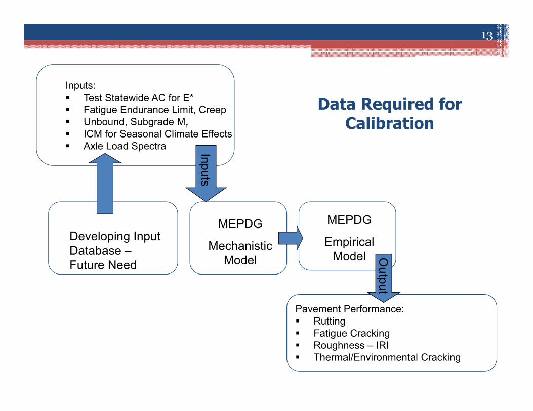
Data Required for Calibration

Inputs: Test Statewide AC for E* Fatigue Endurance Limit, Creep Unbound, Subgrade Mr ICM for Seasonal Climate Effects Axle Load Spectra

Developing InputDatabase –Future Need

MEPDG

Mechanistic Model

MEPDG

Empirical Model

Pavement Performance: Rutting Fatigue Cracking Roughness – IRI Thermal/Environmental Cracking

Output

Inputs

13

Database Development

Database Development

Local Calibration Coefficients

NMDOT

NMDOT Mechanistic Empirical Pavement Design Guide Database

(MEPDG)

DatabaseServer

Phase 1

Database Project Phase

Phase 2

depth21z 0.328196depth)C(C k ××+=

Alli

gato

r Cra

ckin

g (%

)AC Layer Thickness (in)

Calibration

Sensitivity Analysis

14

Development of MEPDG Database

15

Source of MEPDG Oracle Server Setup and Extraction of Data MEPDG Data Population of Data – Example and Analysis Database Security and Maintenance

Outline

16

Source of MEPDG Database

HMMS

MEPDGDSS

TIMS

EMSDBA

SITE MGR PONTIS

TPLC

17

• Local Calibration• Pavement Design• Geographic Information System(GIS) Oriented• Validation of data• Future Database Maintenance• Manage Data more Efficiently• Integrate with analysis• Visualize data• Avoid errors

Benefits of Database to MEPDG

18

Created following proxy Databases to extract data from DMP Files

Oracle Server Setup - Extraction of Data from NMDOT Databases

30 Databases

7 Databases (MEPDG Related)

Extracted Data and Populated

into Local ServerNMDOT

D6PB ( Database Username :- HMMS) DSS (Database Username :-dbuser) FA (Database Username :- EMSDBA) HOSM (Database Username :- SITE_MGR) PONP (Database Username :- PONTIS) TPLC (Database Username :- PLES) TIMS (Database Username :- TIMS)

19

MEPDG Data

Climate

Traffic

Materials

Structure

DistressResponseTime

Damage

Damage Accumulation

20

Database has 5 Categories of data

MEPDG Database’s Main Tables

21

Example of a MEPDG Database Table

22

Example of COUNTY TABLE

23

Traffic Data

• Populated TRAFFIC_COUNT table with data using pythonscript

• Analyzed the Data from TRAFFIC_COUNT table andconverted the data into MEPDG format and stored it inTRAFFIC_NMDOT_GIS Table

• Calculated parameters like General growth rate, Compoundgrowth rate, General growth factor, etc stored inTRAFFIC_GENERAL_GROWTH_RATE table

Population of Data Example

24

New MEPDG Database’s TRAFFIC_COUNT TABLE

25

New MEPDG Database’s TRAFFIC_GENERAL_GROWTH_RATE

26

Axle Load Spectra for Single Axle

0

6

12

18

24

30

0 5000 10000 15000 20000 25000 30000 35000 40000 45000

No

of A

xles

Weight(lb)

00.00 Hrs

01.00 Hrs

02.00 Hrs

03.00 Hrs

04.00 Hrs

05.00 Hrs

06.00 Hrs

27

Axle Load Spectra for Tandem Axles

0

5

10

15

20

25

30

35

0 5000 10000 15000 20000 25000 30000 35000 40000 45000

No

of A

xles

Weight(lb)

00.00 Hrs01.00 Hrs02.00 Hrs03.00 Hrs04.00 Hrs05.00 Hrs06.00 Hrs

28

• FWD (Falling Weight Deflectometer)• Mix Design• Distress• Climate

Other Data Populated

29

• Data Acquisition & Processing

▫ 5900 individual candidate station locations extracted fromNOAA(National Oceanic and Atmospheric Administration) stationlists for NM, AZ, UT, CO, OK, and TX

30

Climate Normal Data

• Candidate stations used to retrieve available data

31

Climate Normal Data

State Number of Full Climate Normal Files

Number of Partial Climate Normal Files

Number of Error Files

Total Number of

Stations Attempted

New Mexico 123 19 567 709

Arizona 148 27 375 550

Utah 159 23 395 577

Colorado 162 33 489 684

Oklahoma 117 82 403 602

Texas 215 134 651 1000

924 318 2880 4122

• Retrieved data include climate normal (i.e. average) dailyvalues based upon period from 1971-2000

▫ Average daily maximum temperature (deg. F)▫ Average daily minimum temperature (deg. F)▫ Average daily mean temperature (deg. F)▫ Average daily precipitation (100ths of inch)▫ Cooling- and Heating-days

32

Climate Normal Data

33

Climate_Normal_Stations Tables

• Database User▫ Not giving full privileges to dbuser to make changes in data tables

• Column Level VPD(Virtual Private Database)▫ Limiting user to access particular columns and other sensitive

information cannot be accessed

• Column-Masking▫ Columns contain sensitive information are returned as NULL values

Database Security and Maintenance

USER PASSWORD DESIGNATION

A NULL Research Assistant

B NULL Research Assistant

C NULL Research Assistant

34

Modules of the MEPDG

• Dynamic (Complex) Modulus (E*)

AC

• Resilient Modulus (Mr)

Unbound Layers

Materials

35

Dynamic (Complex) Modulus |*| E

Dynamic modulus key MEPDG Input E* related to temperature and time rate of loading E* comparable with FWD back calculated modulus

36

Dynamic and Resilient Modulus Test Equipment

GCTS

37

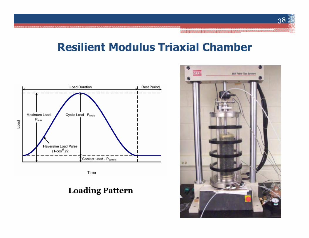
Resilient Modulus Triaxial Chamber

Loading Pattern

38

Sensitivity of MEPDG Inputs Using Advanced Statistical

Analyses

39

Sensitivity

• The study of how the change in outputs of a model can be apportion to thechange in inputs of the model

LowMedium

HighInput OutputMODEL

???

• To understand the impacts and relationships of the hundreds of inputvariables contained in the MEPDG

Example: Effect of aggregate gradation on roughness

• To identify critical points/ most significant risk factorsExample: Which variables are appropriate to prevent cracks

• For a fine-tuned calibration, it is important to analyze the sensitivity ofinput variables

• More appropriate design

• To have an idea about interacting inputs

40

Sensitivity and MEPDG

• Common trend of Sensitivity Analysis is local or changing one factor at a time• Drawbacks:

▫ MEPDG is heavily dependent on a large number of inputs▫ Interaction among inputs are not considered

Goal of this Study Identify , Rank and Quantify the effect of sensitive inputs considering

interaction with others

41

Objective of the Study

• Collect Long Term Pavement Performance (LTPP) and NMDOTmaterials, traffic and climate data, which represent local practice ofNM

• Perform one-to-one sensitivity analysis using New Mexicopavement sections

• Identify and rank a set of MEPDG inputs, sensitive to particulardistress criterion using advanced statistical approaches (such as:linear and nonlinear regression, nonparametric regression)

• Quantify the sensitivity of the inputs considering interactions

42

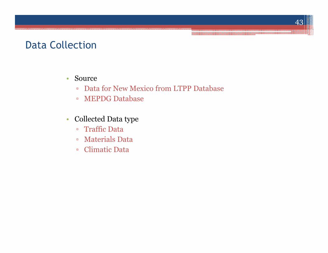
Data Collection

• Source▫ Data for New Mexico from LTPP Database▫ MEPDG Database

• Collected Data type▫ Traffic Data▫ Materials Data▫ Climatic Data

43

Preliminary Sensitivity Analysis

• 14 LTPP sections in New Mexico (12 sections of interstate highway I-25, one section of I-40 and one section of US 550)

• Preparation of sensitivity test matrix with collected data from LTPP database

• 1100 MEPDG simulations using test matrix

• Effects of variables on pavement distresses are identified from the simulation results using line plots, bar plots

44

Test Matrix for Preliminary Sensitivity Analysis

No Variable Range Value

1 Air Void (%) 2 to 10

2 Binder Content 8 to 15

3 Fine Content 2 to 12

4 AC thickness 3 to 10

5 Depth to GWT 2 to 25

6 Operational Speed 15 to 90

7 AADTT 800 to 2000

8 Base Thickness 4 to 18

9 Base Resilient Modulus 15000 to 45000

10 Performance GradePG 58-28, PG 64-28, PG 70-22,

PG 76-22, PG 82-22, AC 20

45

Preliminary Sensitivity Analysis: AC RutA

C R

ut (i

nch)

The input is not showingsame rate of sensitivityfor all test sections0

0.2

0.4

0.6

0.8

1

0 3 6 9 12

Variable Air Void (%)

0

0.2

0.4

0.6

0.8

1

0 1 2 3 4 5 6 7

Performance Grade

46

Preliminary Sensitivity Analysis:Longitudinal Cracking

Long

itudi

nal C

rack

ing

(ft/m

ile) None of the sensitivity

curves exhibit similarpatterns for all testsections

0

400

800

1200

1600

2000

0 3 6 9 12


0

100

200

300

400

2 4 6 8 10 12

AC thickness (in)

47

Preliminary Sensitivity Analysis:Alligator Cracking

Alli

gato

r Cra

ckin

g (%

)

Sensitive toonly one testsection

Sensitive to only few test sections

0

5

10

15

20

25

0 3 6 9 12


0

5

10

15

20

25

3 5 7 9

Binder Content (%)

48

Findings on Preliminary Sensitivity Analysis No Variable Total

RutAC Rut

Terminal IRI

Longitudinal Cracking

Alligator Cracking

1 Air Void (%) S S S S S

2 Binder Content S S LS S S

3 Fineness Content S S LS S LS

4 AC thickness S S S S S

5 Depth to GWT LS LS LS LS LS

6 Operational Speed S S LS LS LS

7 AADTT S S S S S

8 Base Thickness LS LS LS S S

9 Base Resilient Modulus LS LS LS S S

10 Performance Grade S S LS LS S

S = Sensitive, LS = Low Sensitive

Comprehensive analysis of each variableand its interaction with other inputs need tobe fully investigated

49

Advanced Sensitivity Analysis

X1 X2 X3

Input Parameters Distribution

Y = y (x1, x2, x3…...)

Model

Output Distribution

Dy = Estimated variance

√Dy

<y>

Statistical

Methods

SensitivityDy

x2

x1

…x3

50

Flow Chart for SA

Development of Sensitivity Matrix

Defining Inputs and Outputs

Generation of Sample using

Latin Hypercube Sampling Method

Evaluate the Model

MEPDG Simulation

Developing Output

Distribution

Full Test Matrix

Using Statistical Approaches

Test of Correlation

Scatterplot Tests, Linear and Nonlinear Regression

Nonparametric Regression Procedure

Analysis of Results

Identification of Sensitive MEPDG

inputs

Ranking among sensitive inputs

Quantifying the sensitivity of

inputs considering interactionStatistical analyses in this study performed

with R statistical computing environment

51

Defining Inputs and Outputs

• 30 MEPDG input variables are selected of 3 fundamental types

▫ Traffic (X1 to X10)▫ Climate (X11, X12)▫ Materials (X13 to X30)

• 6 output variables from flexible pavement performances (Y1 to Y6)

• A flexible pavement structure is selected

Top AC LayerBottom AC Layer

Base Layer

Subgrade

52

Generation of Sample• Random LHS (Latin Hypercube Sampling) method is followed to generate sample for

an input variable x• x=xi,j where, i=number of sample or nLHS (750), j=data set (30)• During generation of sample, range of each x is divided in nLHS intervals of equal

probability.• Value for xi,j is randomly selected from each of the interval

0

1500

3000

4500

6000

0 150 300 450 600 750

AA

DT

T

No of Sample

Resultant Test Matrix (750 x 30)x =

x1,1 x1,2 x1,3 ………………… x1,30x2,1 x2,2 x2,3 …………………. x2,30………………………………………………….xi,1 ..................... xi,j ……… xi,30…………………………………………………...x750,1 x750,2 ……….………………. x750,30

53

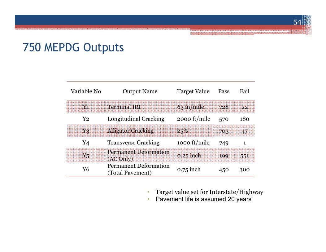
750 MEPDG Outputs

Variable No Output Name Target Value Pass Fail

Y1 Terminal IRI 63 in/mile 728 22

Y2 Longitudinal Cracking 2000 ft/mile 570 180

Y3 Alligator Cracking 25% 703 47

Y4 Transverse Cracking 1000 ft/mile 749 1

Y5 Permanent Deformation (AC Only) 0.25 inch 199 551

Y6 Permanent Deformation (Total Pavement) 0.75 inch 450 300

• Target value set for Interstate/Highway• Pavement life is assumed 20 years

54

0

100

200

300

400

0 150 300 450 600 750

Term

inal

IRI

Distress PredictedDistress TargetInitial IRI

0

5000

10000

15000

0 150 300 450 600 750

Long

itudi

nal C

rack

ing

Distress Predicted Distress Target

0

50

100

150

0 150 300 450 600 750

Allig

ator

Cra

ckin

g

Distress Predicted

Distress Target

Output Distribution

Number of Simulation

55

Output Distribution

0

0.5

1

1.5

0 150 300 450 600 750

AC

Rut


0

500

1000

1500

2000

0 150 300 450 600 750

Tran

sver

se C

rack

ing

Distress PredictedDistress Target

0

1

2

3

0 150 300 450 600 750

Tota

l Rut


Number of Simulation

56

Correlation Test Result

Input Value Type Sign Input Value Type Sign Input Value Type Sign

X1 0.5500 L + X11 0.0800 N + X21 -0.0844 N -X2 0.0325 N + X12 -0.0903 N - X22 0.0784 N +X3 0.1379 S + X13 -0.1660 S - X23 0.0544 N +X4 0.4859 M + X14 0.0169 N + X24 0.0345 N +X5 -0.1172 S - X15 -0.0104 N - X25 -0.0944 N -X6 0.0455 N + X16 -0.0615 N - X26 -0.1346 S -X7 -0.0426 N - X17 0.1185 S + X27 -0.2207 S -X8 0.1555 S + X18 -0.3253 M - X28 0.0210 N +X9 -0.0261 N - X19 -0.0579 N - X29 0.0079 N +

X10 0.1873 S + X20 0.1109 S + X30 -0.1421 S -

Output Y6 (Total Rut)

N= None, S=Small, M=Medium, L=Large, (+)=Positive, (-)=NegativeN=(0.0 to 0.09)/(-0.09 to 0.0), S=(0.1 to 0.3)/(-0.3 to -0.1), M=(0.3 to 0.5)/(-0.5 to -0.03), L=(0.5 to 1.0)/(-1.0.5 to-0.5)

57

Correlation Test Result (Cont.)

0

1

2

3

0 1500 3000 4500 6000

0

1

2

3

0 25 50 75 1000

1

2

3

2 4 6 8


Percent of Trucks in Design Lane (%) (X4)

Initial two-way AADTT (X1)

Asphalt Layer Thickness (bottom Layer) (X18)

Tota

l Rut

(inc

h)

58

Scatterplots

• Common Means (CMN)• Common Locations (CL)• Statistical Independence (SI)• Linear Regression (REG)• Quadratic Regression (QREG)• Rank Correlation Coefficient (RCC)• Squared Rank Differences (SRD)• Combining Statistical (SRD/RCC)

Test Methods

59

Input Ranking

Test CMN Results CL Results SI Results REG Results

Rank Input p-value Input p-value Input p-value Input p-value

1 X18 0.0000 X1 0.0000 X1 0.0000 X18 0.0000

2 X1 0.0000 X4 0.0000 X4 0.0000 X1 0.0000

3 X4 0.0000 X18 0.0000 X18 0.0000 X4 0.0000

4 X13 0.0000 X26 0.0000 X26 0.0000 X13 0.0000

5 X26 0.0001 X27 0.0000 X13 0.0003 X27 0.0000

6 X27 0.0001 X13 0.0002 X10 0.0005 X26 0.0000

7 X25 0.0003 X10 0.0005 X27 0.0033 X25 0.0000

8 X22 0.0031 X3 0.0020 X8 0.0089 X22 0.0001

9 X3 0.0056 X5 0.0031 X17 0.0400 X3 0.0009

10 X8 0.0234 X8 0.0032 X5 0.0400 X10 0.0037

11 X10 0.0368 X30 0.0166 X29 0.0495 X8 0.0040

12 X9 0.0479 X17 0.0203

13 X30 0.0292

14 X5 0.0492

Output Y1=Terminal IRI

Level of Significance = 0.05

60

Input Ranking (Cont.)

Test QREG Results RCC Results SRD Results SRD/RCC Results

Rank Input p-value Input p-value Input p-value Input p-value

1 X1 0.0000 X1 0.0000 X4 0.0000 X1 0.0000

2 X4 0.0000 X4 0.0000 X1 0.0000 X4 0.0000

3 X18 0.0000 X18 0.0000 X18 0.0001 X18 0.0000

4 X13 0.0000 X26 0.0000 X26 0.0000

5 X26 0.0000 X27 0.0000 X27 0.0000

6 X27 0.0000 X13 0.0000 X13 0.0000

7 X25 0.0001 X10 0.0000 X10 0.0000

8 X22 0.0003 X8 0.0003 X5 0.0008

9 X3 0.0033 X3 0.0009 X8 0.0010

10 X5 0.0039 X5 0.0013 X3 0.0045

11 X8 0.0076 X30 0.0033 X30 0.0048

12 X10 0.0114 X17 0.0083 X17 0.0226

13 X30 0.0182 X22 0.0120 X25 0.0320

14 X9 0.0272 X12 0.0126 X12 0.0399

15 X25 0.0232 X11 0.0444

16 X11 0.0242

Output Y1=Terminal IRI

Leve

l of S

igni

fican

ce =

0.0

5

61

Identified Sensitive Inputs

Name of Test CMN CL SI REG QREG RCC SRD SRD/RCC

Terminal IRI

X18X1X4X13

X1X4X18X26

X1X4X18X26

X18X1X4X13

X1X4X18X13

X1X4X18X26X27

X1X4

X1X4X18X26X27

LongitudinalCracking

X18X4X1X24X25

X18X1X4X27X24X25X13

X18X4X1X27

X18X4X1X25X17

X18X4X1X25X17

X18X4X1X27X25X13X17

X18 X18X1X4X27X25X13X17

AlligatorCracking

X18X1X4X22X13

X18X4X1X22X13

X18X1X4

X18X1X4X22X13X25

X18X1X4X22X13X25

X18X4X1X22X13

X18X4

X1X4X18X22X13

62

Identified Sensitive Inputs (Cont.)

Name of Test CMN CL SI REG QREG RCC SRD SRD/RCC

TransverseCracking

N/A N/A X14X19X21X16X2

N/A N/A N/A N/A N/A

AC Rut

X1X4X10X18X8

X1X4X10X18

X1X4X10

X1X4X10X18X8

X1X4X10X18X8

X1X4X10X18X8

X1X4

X1X4X10X18X8

Total Rut

X1X4X18X27

X1X4X18X27

X1X4X18X26

X1X4X18X27X10X13

X1X4X18X27X10

X1X4X18X27X10

X1X4

X1X4X18X27X10

63

Most Important Inputs

Output 1 2 3 4Terminal IRI Bottom AC layer

ThicknessAADTT Percent of trucks

in design laneType of subgradeMaterial

Longitudinal Cracking Bottom AC layer Thickness

Percent of trucks in design lane

AADTT Modulus of Subgrade Layer

Alligator Cracking Bottom AC layer Thickness

AADTT Percent of trucks in design lane

Percent air void of bottom AC layer

Transverse CrackingGradation of Top AC layer

Gradation of Bottom AC layer

PG grade of bottom ac layer

PG grade of top ac layer

AC Rut AADTT Percent of trucks in design lane

Tire pressure Bottom AC layer Thickness

Total Rut AADTT Percent of trucks in design lane

Bottom AC layer Thickness

Modulus of subgrade

64

Linear Regression

Input Name R2 Increment R2 (%)

SRC PCC2 95% PCC2 CI p-Value

X18AC Layer Thickness (2nd AC Layer)

0.311 31 -0.547 0.424 (0.382, 0.487) 0.000

X4Percent of Trucks in Design Lane (%)

0.383 7 0.251 0.134 (0.097, 0.188) 0.000

X1 AADTT 0.440 6 0.239 0.124 (0.081, 0.171) 0.000

X24 Base Material Type 0.484 4 0.197 0.087 (0.055, 0.134) 0.000

X17 Air Void (%) (Top AC Layer) 0.518 3 0.178 0.072 (0.042, 0.112) 0.000

X25 Base Modulus 0.543 3 -0.154 0.055 (0.026, 0.089) 0.000

X13 AC Layer Thickness (Top Layer) 0.562 2 -0.139 0.046 (0.023, 0.085) 0.000

X27 Subgrade Modulus 0.576 1 0.124 0.036 (0.013, 0.068) 0.000

X15Effective binder content (%) (Top AC Layer)

0.586 1 -0.094 0.021 (0.004, 0.046) 0.021

X23 Base Thickness 0.594 1 -0.088 0.019 (0.000, 0.041) 0.027

X3Percent of Trucks in Design Direction (%)

0.597 0 0.057 0.008 (0.000, 0.029) 0.195

Output Y2 (Longitudinal Cracking)

SRC = Standardized Regression CoefficientPCC = Partial Correlation Coefficient

65

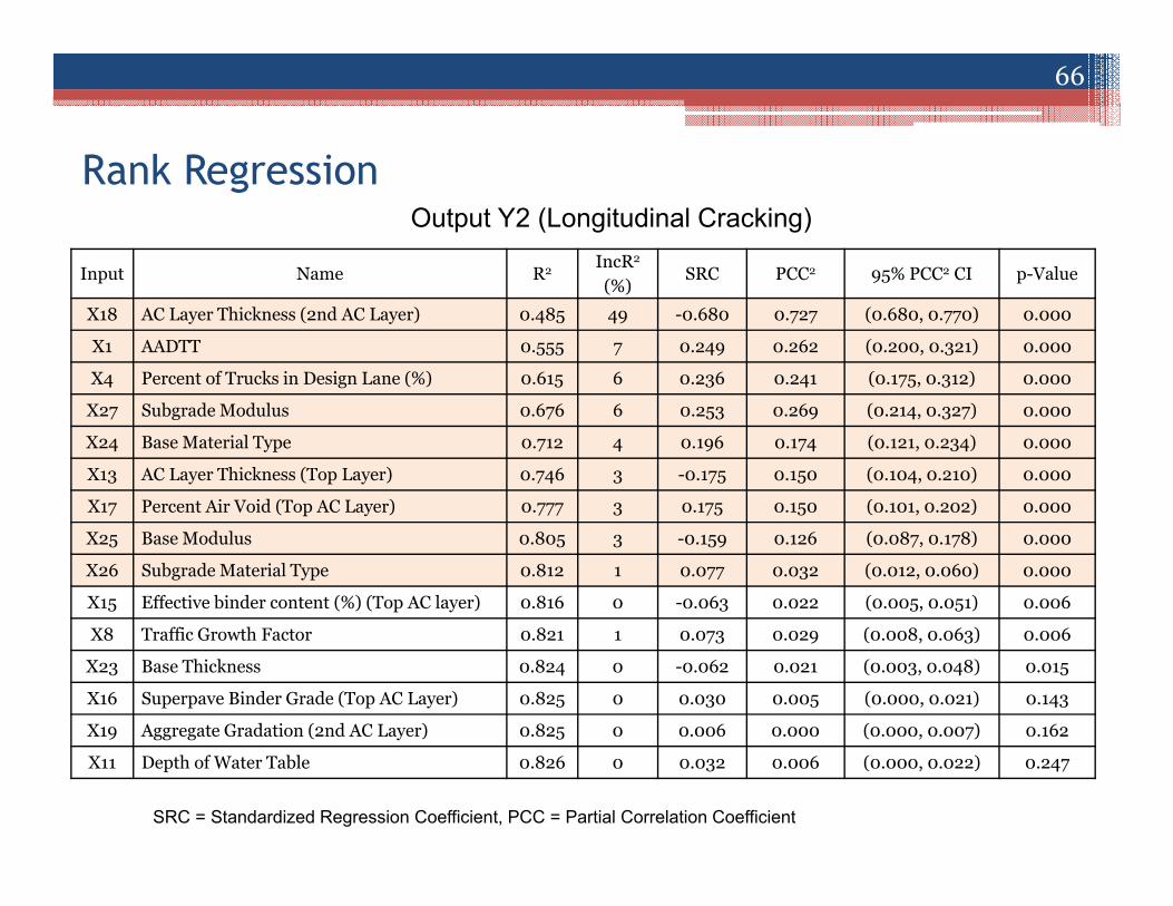
Rank Regression

Input Name R2 IncR2

(%)SRC PCC2 95% PCC2 CI p-Value

X18 AC Layer Thickness (2nd AC Layer) 0.485 49 -0.680 0.727 (0.680, 0.770) 0.000

X1 AADTT 0.555 7 0.249 0.262 (0.200, 0.321) 0.000

X4 Percent of Trucks in Design Lane (%) 0.615 6 0.236 0.241 (0.175, 0.312) 0.000

X27 Subgrade Modulus 0.676 6 0.253 0.269 (0.214, 0.327) 0.000

X24 Base Material Type 0.712 4 0.196 0.174 (0.121, 0.234) 0.000

X13 AC Layer Thickness (Top Layer) 0.746 3 -0.175 0.150 (0.104, 0.210) 0.000

X17 Percent Air Void (Top AC Layer) 0.777 3 0.175 0.150 (0.101, 0.202) 0.000

X25 Base Modulus 0.805 3 -0.159 0.126 (0.087, 0.178) 0.000

X26 Subgrade Material Type 0.812 1 0.077 0.032 (0.012, 0.060) 0.000

X15 Effective binder content (%) (Top AC layer) 0.816 0 -0.063 0.022 (0.005, 0.051) 0.006

X8 Traffic Growth Factor 0.821 1 0.073 0.029 (0.008, 0.063) 0.006

X23 Base Thickness 0.824 0 -0.062 0.021 (0.003, 0.048) 0.015

X16 Superpave Binder Grade (Top AC Layer) 0.825 0 0.030 0.005 (0.000, 0.021) 0.143

X19 Aggregate Gradation (2nd AC Layer) 0.825 0 0.006 0.000 (0.000, 0.007) 0.162

X11 Depth of Water Table 0.826 0 0.032 0.006 (0.000, 0.022) 0.247

Output Y2 (Longitudinal Cracking)

SRC = Standardized Regression Coefficient, PCC = Partial Correlation Coefficient

66

Summary of Regression Analysis

Model Name Linear Regression Rank Regression

R2 ≥10% 6-9% 3-5% ≤2% R2 ≥10% 6-9% 3-5% ≤2%

Y1 Terminal IRI

0.61 X18, X1

X4, X13

X26, X27, X30, X22, X10, X25, X8

0.85 X1, X4, X18

X26, X27, X10, X30

X13, X8, X3,

X29, X5,

X22, X12, X24

Y2 Longitudinal Cracking

0.61 X18 X4, X1

X24, X17, X25

X13, X27, X15, X23

0.84 X18 X1, X4, X27

X24, X13, X17, X25

X26, X8

Y3 Alligator Cracking

0.51 X18 X1 X4, X22, X13

X25, X24, X12, X27, X3

0.88 X18, X4, X1

X22, X13

X20, X24, X8,

X25, X27, X3

67

Summary of Regression Analysis

Model Name Linear Regression Rank Regression

R2 ≥10% 6-9% 3-5% ≤2% R2 ≥10% 6-9% 3-5% ≤2%

Y4 Transverse Cracking

0.01 X24 0.07 X16, X12, X24

Y5 Permanent Deformation (AC Only)

0.86 X1, X4

X10 X8, X18

X12, X13, X6, X16, X3,

X30, X5

0.88 X1, X4

X10 X18, X8

X12, X13, X5, X16, X3,

X30, X6

Y6 Permanent Deformation (Total Pavement)

0.85 X1, X4, X18

X27, X10, X30

X8, X13, X26, X12, X3, X5

0.86 X1, X4

X18 X10, X27, X30, X8

X26, X13, X12, X3, X5

68

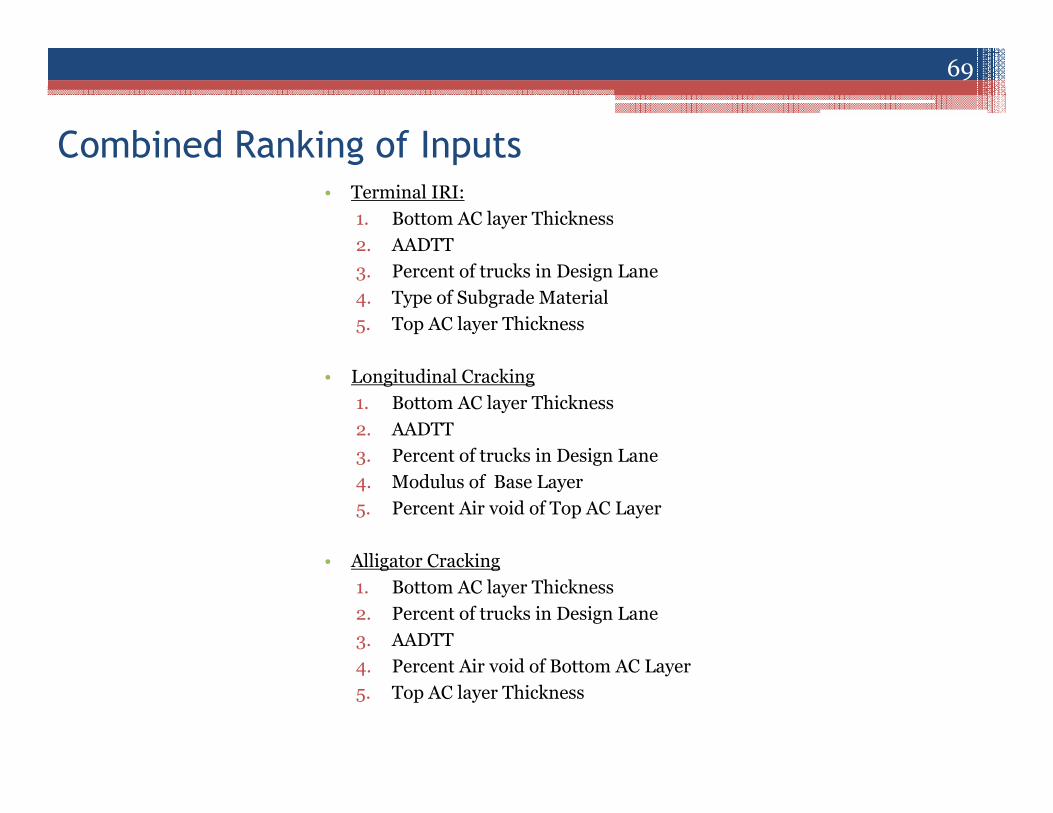
Combined Ranking of Inputs• Terminal IRI:

1. Bottom AC layer Thickness2. AADTT3. Percent of trucks in Design Lane4. Type of Subgrade Material5. Top AC layer Thickness

• Longitudinal Cracking1. Bottom AC layer Thickness2. AADTT3. Percent of trucks in Design Lane4. Modulus of Base Layer5. Percent Air void of Top AC Layer

• Alligator Cracking1. Bottom AC layer Thickness2. Percent of trucks in Design Lane3. AADTT4. Percent Air void of Bottom AC Layer5. Top AC layer Thickness

69

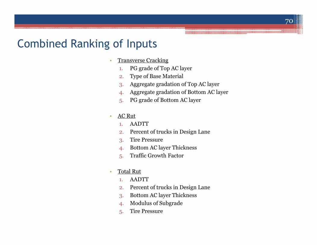
Combined Ranking of Inputs• Transverse Cracking

1. PG grade of Top AC layer2. Type of Base Material3. Aggregate gradation of Top AC layer4. Aggregate gradation of Bottom AC layer5. PG grade of Bottom AC layer

• AC Rut1. AADTT2. Percent of trucks in Design Lane3. Tire Pressure4. Bottom AC layer Thickness 5. Traffic Growth Factor

• Total Rut1. AADTT2. Percent of trucks in Design Lane3. Bottom AC layer Thickness4. Modulus of Subgrade5. Tire Pressure

70

Nonparametric Regression Procedure• Nonparametric Regression Procedures are used to estimate the necessary

sensitivity index for each input

▫ Quadratic Response Surface Regression (QREG)▫ Multivariate Adaptive Regression Splines (MARS)▫ Gradient Boosting Machine (GBM)

• Single Variance Index (S) and Total variance Index (T) are calculated using theseprocedures

Fraction of Uncertainty due to

xj aloneS

SInteractions of

xj with other variables

T

71

QREG Results

Input Name S.hat T.hat Interactions 95% T CI p-value

X18 AC Layer Thickness (2nd AC Layer)

0.380 0.600 0.220 (0.576, 0.671) 0.000

X1 AADTT 0.148 0.187 0.039 (0.156, 0.248) 0.000

X22 Air Void (%) (AC 2nd Layer)

0.091 0.121 0.030 (0.093, 0.174) 0.000

X4 Percent of Trucks in Design Lane (%)

0.103 0.115 0.012 (0.067, 0.150) 0.000

X13 AC Layer Thickness (Top Layer)

0.088 0.088 0.000 (0.045, 0.126) 0.000

X24 Base Material Type 0.037 0.050 0.013 (0.012, 0.095) 0.004

X25 Base Modulus 0.052 0.052 0.000 (0.006, 0.082) 0.015

Y3 (Alligator Cracking)

S = Single Variance IndexT = Total Variance Index

72

MARS Result



0.049 0.874 0.825 (0.026, 1.000) 0.000

X7 AADTT Distribution by Vehicle Class 11 (%)

0.354 0.406 0.052 (0.194, 0.812) 0.013

Y4 (Transverse Cracking)


73

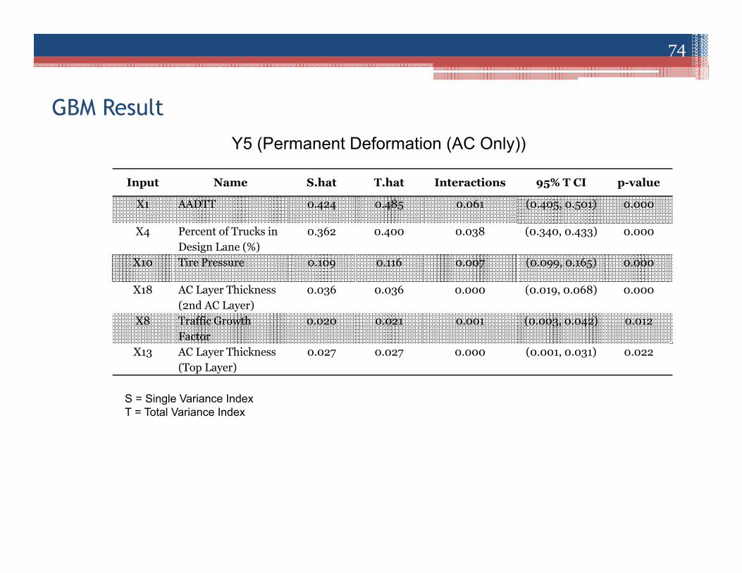
GBM Result


X1 AADTT 0.424 0.485 0.061 (0.405, 0.501) 0.000


0.362 0.400 0.038 (0.340, 0.433) 0.000

X10 Tire Pressure 0.109 0.116 0.007 (0.099, 0.165) 0.000

X18 AC Layer Thickness (2nd AC Layer)

0.036 0.036 0.000 (0.019, 0.068) 0.000

X8 Traffic Growth Factor

0.020 0.021 0.001 (0.003, 0.042) 0.012

X13 AC Layer Thickness (Top Layer)

0.027 0.027 0.000 (0.001, 0.031) 0.022

Y5 (Permanent Deformation (AC Only))


74

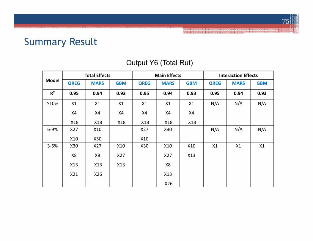
Summary Result

ModelTotal Effects Main Effects Interaction Effects

QREG MARS GBM QREG MARS GBM QREG MARS GBM

R2 0.95 0.94 0.93 0.95 0.94 0.93 0.95 0.94 0.93

≥10% X1

X4

X18

X1

X4

X18

X1

X4

X18

X1

X4

X18

X1

X4

X18

X1

X4

X18

N/A N/A N/A

6-9% X27

X10

X10

X30

X27

X10

X30 N/A N/A N/A

3-5% X30

X8

X13

X21

X27

X8

X13

X26

X10

X27

X13

X30 X10

X27

X8

X13

X26

X10

X13

X1 X1 X1


75

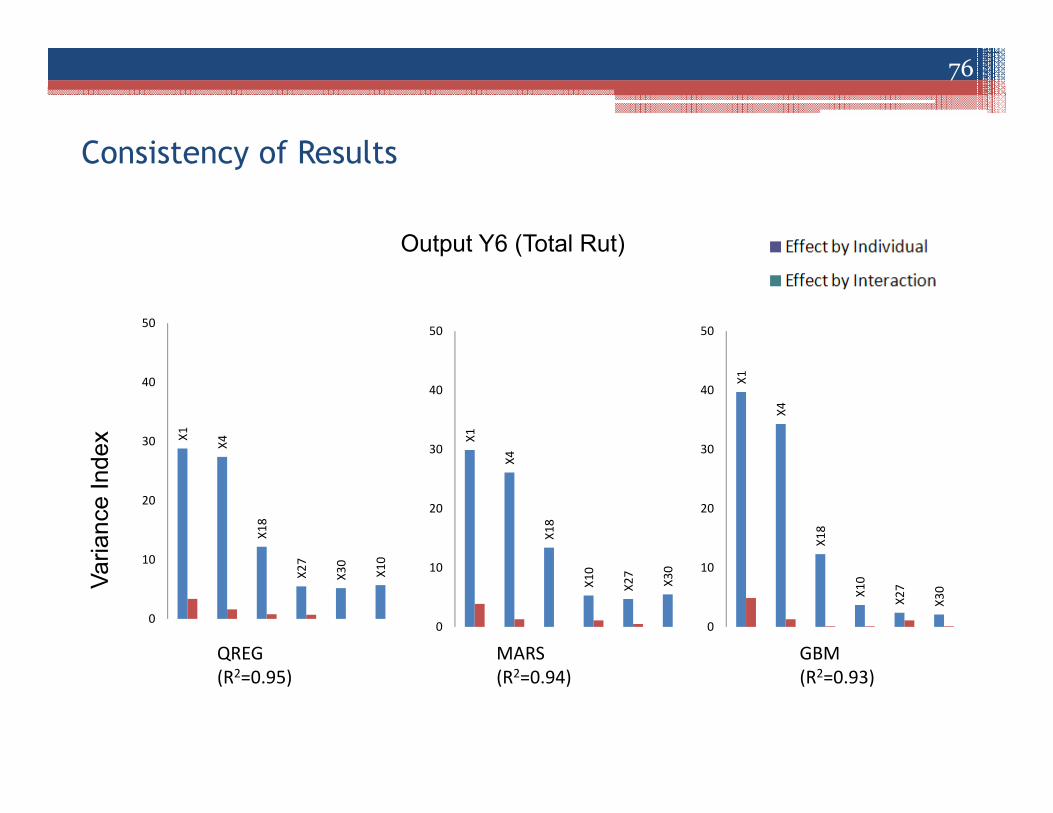
Consistency of Results

QREG (R2=0.95)

MARS(R2=0.94)

GBM(R2=0.93)


X1 X4

X18

X27

X30

X10

0

10

20

30

40

50

X1

X4

X18

X10

X27

X30

0

10

20

30

40

50

X1

X4

X18

X10

X27

X30

0

10

20

30

40

50

Varia

nce

Inde

x76

Consistency of Results (Cont.)

▫ Total variance index obtained in 3 cases are close to each other

▫ Range of 95% CI are almost similar in all cases

QREGMARS

GBM

0

10

20

30

40

50

QREG MARS GBM

0

5

10

15

20

X10 (Tire Pressure)

X4 (Percent of Trucks in Design Lane)

X18 (Bottom AC Layer Thickness)

Tota

l Var

ianc

e In

dex,

T (%

)


QREG

MARS

GBM

0

3

6

9

12

77

Remarks• High Sensitive Inputs:

▫ Terminal IRI: Bottom AC layer Thickness, AADTT and percent of trucks in designlane

▫ Longitudinal Cracking: Bottom AC layer Thickness, AADTT and Percent of trucksin Design Lane

▫ Alligator Cracking: Bottom AC layer Thickness, AADTT and Percent Air void ofBottom AC Layer

▫ Transverse cracking: AADTT and Percent of Vehicle class 11

▫ AC Rut: AADTT, Percent of trucks in Design Lane and Tire Pressure

▫ Total Rut: AADTT, Percent of trucks in Design Lane and Bottom AC layerThickness

78

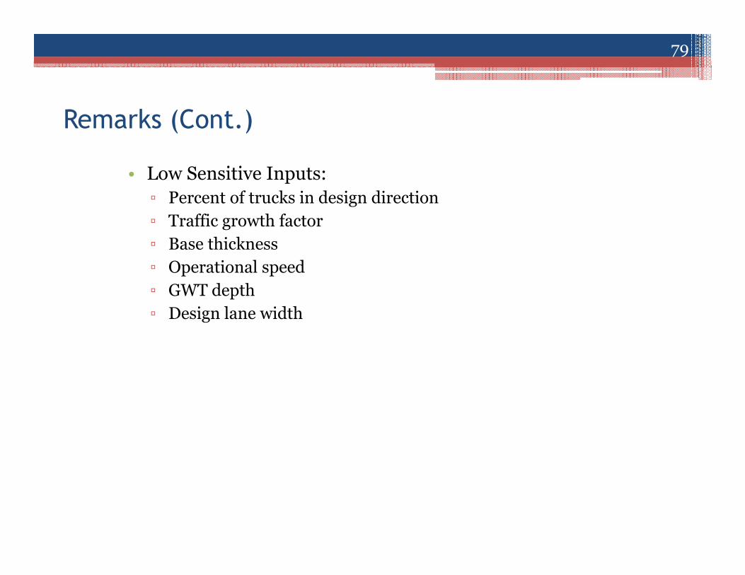
Remarks (Cont.)

• Low Sensitive Inputs:▫ Percent of trucks in design direction▫ Traffic growth factor▫ Base thickness▫ Operational speed▫ GWT depth▫ Design lane width

79

Remarks (Cont.)

• Traffic input variables, such as Annual Average Daily Truck Traffic(AADTT) and Percent of Trucks in Design Lane are obtained to bethe most critical parameter

• For New Mexico, AC mix properties and AC thickness are veryimportant for roughness, longitudinal crack and fatigue crack. Baseproperties (modulus and thickness) have significant impact on longand fatigue crack

• Most interactive input is Bottom AC layer thickness

80

Local Calibration of MEPDG

81

DATA FOR LOCAL CALIBRATIO

Local Calibration Performed using both

- LTPP pavement sections (11 data) - PMS data (13 data)

82

Calibration ≡ Find a set of calibration coefficients that minimizes the residual error

Validation is the process necessary to confirm that the new models work for cases different to those used in

calibration

Calibration and Validation

Target: Minimize the Sum of Squared Errors (SSE)( )2 −= istresspredictedDstressmeasuredDiSSE

Split-sample approach: 80% of pavement sections are used for calibration and 20% for validation (randomly chosen)

83

MEPDG Inputs and Outputs

TrafficClimate

MaterialsMEPDG

RuttingCracking

Roughness

INPUTS OUTPUTS

• 13 sections from NMDOT databases• 11 sections from LTPP database

84

Calibration Data

SHRP

IdRoad MP

Type of

Experiment

Constructio

n Date *

1002

1003

1005

1022

1112

2006

2007

2118

6033

6035

6401

US-70

US-70

I-25

US-550

US-62

US-550

US-550

I-40

I-25

I-40

I-40

310.1

320.9

263.8

125.1

81.3

89.5

106.2

346.2

159.3

96.7

107.7

GPS-6A

GPS-1

GPS-1

GPS-1

GPS-1

GPS-2

GPS-6A

GPS-2

GPS-6A

GPS-6A

GPS-6A

May, 1985

May, 1983

Sep, 1983

Sep, 1986

May, 1984

Jun, 1982

Jun, 1981

Dec, 1979

May, 1981

May, 1985

May, 1984

GPS-1,2 = AC on GBGPS-6A = AC overlay on AC

Section

#Road Milepoint

Type of

Section

Construction

Date *

NMDOT 2

NMDOT 4

NMDOT 5

NMDOT 6

NMDOT 10

NMDOT 12

NMDOT 15

NMDOT 19

NMDOT 20

NMDOT 21

NMDOT 23

NMDOT 25

NMDOT 27

I-10

I-40

I-40

I-40

I-25

US-54

US-62

US-64

US-64

US-70

US-82

US-84

US-180

148.0

183.0

187.0

243.0

252.0

82.0

35.0

97.0

205.0

254.0

135.0

183.0

114.0

Rehab.

New

New

Rehab.

New

New

New

Rehab.

New

New

New

Rehab.

New

07/1984

06/1999

06/1999

06/1986

07/1982

06/1977

05/1992

10/1983

10/1971

10/1986

09/1994

07/1985

09/1994* Date of last major improvement in the case of rehabilitated sections

13 NMDOT sections 11 LTPP sections

85

MEPDG model for prediction of total rutting:

(Rut in AC)

(Rut in GB)

(Rut in SG)

hAC, hGB, hSG = Thickness of layer (in)T = Pavement temperature (F)N = Number of load repetitionsεr = Resilient strainεv = Average vertical strainε0, β, ρ = Material properties

kZ = Factor that depends on hAC and depth of point where strain is being determinedk1 = -3.35412, k2 = 1.5606, k3 = 0.4791kGB = 2.03, kSG = 1.35βr1, βr2, βr3, βGB, βSG = Calibration coefficients

Permanent Deformation Model

332211

1

10 rkrkkzrACr

layers

i

ip

i NTkhhRut ββεβε ⋅⋅

=

⋅⋅⋅⋅⋅⋅=⋅= βρ

εεεβ

−

⋅⋅⋅⋅⋅+ N

rGBvGBGB ekh 0

βρ

εεεβ

−

⋅⋅⋅⋅⋅+ N

rSGvSGSG ekh 0

86

MEPDG RUTTING MODEL• Asphalt Concrete Rutting Model:

87

MEPDG RUTTING MODEL• Unbound Materials and Subgrade Rutting Model:

88

Only total rutting can be calibrated. Calibration of βr1, βr2, βr3, βGB, and βSG separately for each layer would require cutting trenches to measure the rut depth in

every layer

The application of nonlinear numerical optimization was considered but the problem would become too difficult because MEPDG uses a complex iterative process

For every ∆t, incremental distresses due to N and T at that particular time are cumulated and materials strength

changes due to temperature and moisture, then next step starts

Calibration of the Rutting Model

89

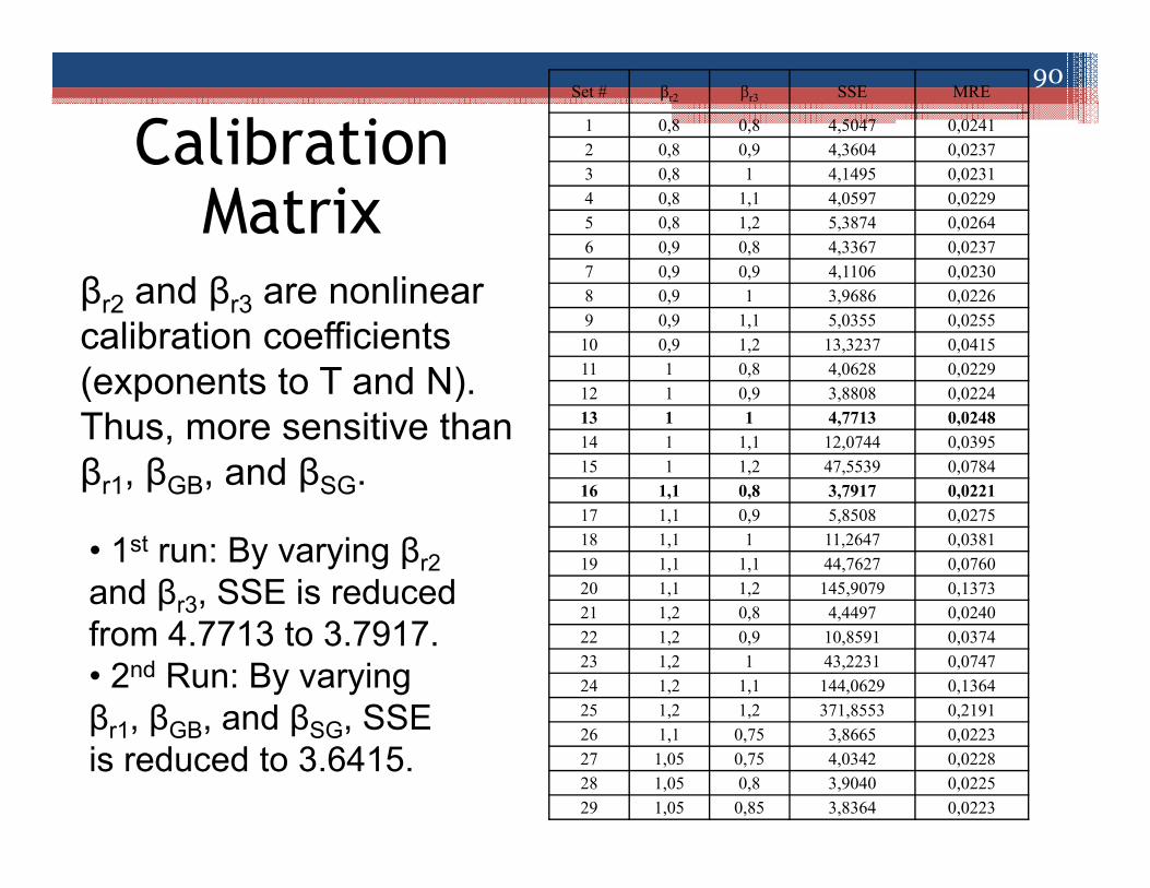
Calibration Matrix

βr2 and βr3 are nonlinear calibration coefficients (exponents to T and N).Thus, more sensitive thanβr1, βGB, and βSG.

• 1st run: By varying βr2and βr3, SSE is reduced from 4.7713 to 3.7917.• 2nd Run: By varying βr1, βGB, and βSG, SSE is reduced to 3.6415.

Set # βr2 βr3 SSE MRE

1 0,8 0,8 4,5047 0,02412 0,8 0,9 4,3604 0,02373 0,8 1 4,1495 0,02314 0,8 1,1 4,0597 0,02295 0,8 1,2 5,3874 0,02646 0,9 0,8 4,3367 0,02377 0,9 0,9 4,1106 0,02308 0,9 1 3,9686 0,02269 0,9 1,1 5,0355 0,025510 0,9 1,2 13,3237 0,041511 1 0,8 4,0628 0,022912 1 0,9 3,8808 0,022413 1 1 4,7713 0,024814 1 1,1 12,0744 0,039515 1 1,2 47,5539 0,078416 1,1 0,8 3,7917 0,022117 1,1 0,9 5,8508 0,027518 1,1 1 11,2647 0,038119 1,1 1,1 44,7627 0,076020 1,1 1,2 145,9079 0,137321 1,2 0,8 4,4497 0,024022 1,2 0,9 10,8591 0,037423 1,2 1 43,2231 0,074724 1,2 1,1 144,0629 0,136425 1,2 1,2 371,8553 0,219126 1,1 0,75 3,8665 0,022327 1,05 0,75 4,0342 0,022828 1,05 0,8 3,9040 0,022529 1,05 0,85 3,8364 0,0223

90

Coefficients β1 = 1.1, β2 = 1.1, β3 = 0.8, βGB = 0.8, and βSG = 1.2 reduces the SSE from 4.7713 to 3.6415.

After calibration, data is less scattered and closer to the line

Results

0

0.1

0.2

0.3

0.4

0.5

0.6

0.7

0.8

0.9

1

0 0.1 0.2 0.3 0.4 0.5 0.6 0.7 0.8 0.9 1

Pred

icte

d To

tal R

uttin

g (in

)

Measured Total Rutting (in)

LTPP Sections

0

0.1

0.2

0.3

0.4

0.5

0.6

0.7

0.8

0.9

1

0 0.1 0.2 0.3 0.4 0.5 0.6 0.7 0.8 0.9 1Pr

edic

ted

Tota

l Rut

ting

(in)

Measured Total Rutting (in)

LTPP SectionsNMDOT SectionsLinear (Line of Equality)

Uncalibrated Calibrated

91

Sections 2006, 6033, NMDOT 15, NMDOT 21, and NMDOT 25 are kept aside for validation. The new model improves the MEPDG prediction, the SSE

decreases from 0.3064 to 0.1142

Rutting Model Validation

0

0.1

0.2

0.3

0.4

0.5

0.6

0.7

0.8

0 5 10 15 20 25

Tota

l Rut

ting

(in)

Design Life (years)

Measured

Uncalibrated

Calibrated

NMDOT 25

92

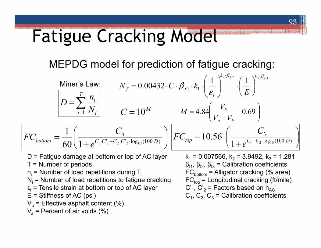
Fatigue Cracking ModelMEPDG model for prediction of fatigue cracking:

Miner’s Law:

D = Fatigue damage at bottom or top of AC layerT = Number of periodsni = Number of load repetitions during TiNi = Number of load repetitions to fatigue crackingεt = Tensile strain at bottom or top of AC layerE = Stiffness of AC (psi)Vb = Effective asphalt content (%)Va = Percent of air voids (%)

k1 = 0.007566, k2 = 3.9492, k3 = 1.281βf1, βf2, βf3 = Calibration coefficientsFCbottom = Alligator cracking (% area)FCtop = Longitudinal cracking (ft/mile)C’1, C’2 = Factors based on hACC1, C2, C3 = Calibration coefficients

=

=T

i i

i

NnD

1

3322 1100432.0 11

ff kk

tff EkCN

ββ

εβ

⋅⋅

⋅

⋅⋅⋅⋅=

MC 10=

−

+= 69.084.4

ba

b

VVVM

+= ⋅⋅⋅+⋅ )100(log''

3102211160

1DCCCCbottom e

CFC

+⋅= ⋅⋅− )100(log

310211

56.10 DCCtop eCFC

93

MEPDG FATIGUE CRACKING MODEL

• Fatigue Damage Model:

94

MEPDG FATIGUE CRACKING MODEL• Bottom-Up and Top-Down Cracking Model:

95

Bottom Up Cracking:Calibration Matrix

Calibration coefficients βf1, βf2, and βf3 are not calibrated

because the number of load repetitions necessary to initiate

fatigue damage is unknown

By varying C1 and C2, the SSE is reduced from 4861.47 to 3537.84The coefficient C3 is fixed at the default value 6000

Set # C1 C2 C3 SSE MRE

1 0.25 0.25 6000 15082.72 1.622 0.25 0.625 6000 18217.61 1.783 0.25 1 6000 27329.87 2.184 0.25 1.5 6000 39688.19 2.625 0.25 2 6000 48542.23 2.906 0.625 0.25 6000 3537.84 0.787 0.625 0.625 6000 4184.23 0.858 0.625 1 6000 5729.43 1.009 0.625 1.5 6000 12219.83 1.4510 0.625 2 6000 23157.53 2.0011 1 0.25 6000 4876.49 0.9212 1 0.625 6000 4918.98 0.9213 1 1 6000 4861.47 0.9214 1 1.5 6000 4977.75 0.9315 1 2 6000 7220.50 1.1216 1.5 0.25 6000 5219.85 0.9517 1.5 0.625 6000 5223.26 0.9518 1.5 1 6000 5211.96 0.9519 1.5 1.5 6000 5163.09 0.9520 1.5 2 6000 5044.81 0.9321 2 0.25 6000 5251.35 0.9522 2 0.625 6000 5251.13 0.9523 2 1 6000 5249.79 0.9524 2 1.5 6000 5245.37 0.9525 2 2 6000 5231 29 0 95

96

Coefficients C1 = 0.625, C2 = 0.25 and C3 = 6000 reduce the SSE from 4861.47 to 3537.84. Data points get closer to line of equality

Results: Bottom Up Cracking

0

5

10

15

20

25

0 5 10 15 20 25

Pred

icte

d A

lliga

tor C

rack

ing

(%)

Measured Alligator Cracking (%)

LTPP Sections

NMDOT Sections

0

5

10

15

20

25

0 5 10 15 20 25Pr

edic

ted

Alli

gato

r Cra

ckin

g (%

)Measured Alligator Cracking (%)

LTPP Sections

NMDOT Sections


97

Alligator Cracking Validation

Sections 1002, 1022, NMDOT 19, NMDOT 20, and NMDOT 27 are kept aside for validation. The new model improves the MEPDG prediction, the SSE decreases from 183.60 to 76.16

0

2

4

6

8

10

12

0 5 10 15

Alli

gato

r Cra

ckin

g (%

)

Design Life (years)

Measured

Uncalibrated

CalibratedNMDOT 27

98

Fatigue Cracking ModelMEPDG model for prediction of fatigue cracking:

Miner’s Law:

D = Fatigue damage at bottom or top of AC layerT = Number of periodsni = Number of load repetitions during TiNi = Number of load repetitions to fatigue crackingεt = Tensile strain at bottom or top of AC layerE = Stiffness of AC (psi)Vb = Effective asphalt content (%)Va = Percent of air voids (%)

k1 = 0.007566, k2 = 3.9492, k3 = 1.281βf1, βf2, βf3 = Calibration coefficientsFCbottom = Alligator cracking (% area)FCtop = Longitudinal cracking (ft/mile)C’1, C’2 = Factors based on hACC1, C2, C3 = Calibration coefficients

=

=T

i i

i

NnD

1

3322 1100432.0 11

ff kk

tff EkCN

ββ

εβ

⋅⋅

⋅

⋅⋅⋅⋅=

MC 10=

−

+= 69.084.4

ba

b

VVVM

+= ⋅⋅⋅+⋅ )100(log''

3102211160

1DCCCCbottom e

CFC

+⋅= ⋅⋅− )100(log

310211

56.10 DCCtop eCFC

99

Top Down Cracking:Calibration Matrix

By varying C1 and C2, the SSE is reduced from 603,101,012.34 to 58,406,192.29

The coefficient C3 is fixed at the default value 1000

Set # C1 C2 C3 SSE MRE

1 1 0.3 1000 645,006,970.17 285.362 1 1 1000 1,660,586,371.17 457.873 1 2.25 1000 3,306,382,014.97 646.084 1 3.5 1000 4,131,306,348.15 722.195 1 5 1000 4,704,069,017.36 770.636 3 0.3 1000 58,406,192.29 85.877 3 1 1000 164,870,343.26 144.278 3 2.25 1000 1,369,715,531.19 415.849 3 3.5 1000 2,569,406,002.47 569.5410 3 5 1000 3,365,469,711.99 651.8311 5 0.3 1000 94,519,508.65 109.2412 5 1 1000 82,731,955.85 102.2013 5 2.25 1000 385,880,672.89 220.7214 5 3.5 1000 1,370,064,827.49 415.8915 5 5 1000 2,462,362,046.06 557.5516 7 0.3 1000 104,188,084.77 114.6917 7 1 1000 101,542,737.84 113.2218 7 2.25 1000 112,599,922.33 119.2319 7 3.5 1000 603,101,012.34 275.9320 7 5 1000 1,545,935,462.19 441.7821 10 0.3 1000 1,545,935,462.19 115.5422 10 1 1000 105,597,022.35 115.4623 10 2.25 1000 103,391,480.45 114.2524 10 3.5 1000 147,298,191.72 136.3725 10 5 1000 646,631,817.72 285.72

100

Coefficients C1 = 3, C2 = 0.3 and C3 = 1000 reduce the SSE from 603,101,012.34 to 58,406,192.29. Data points get close to the line of equality and much better agreement is obtained

Results

0

1000

2000

3000

4000

5000

6000

0 1000 2000 3000 4000 5000 6000

Pred

icte

d Lo

ngitu

dina

l Cra

ckin

g (f

t/mi)

Measured Longitudinal Cracking (ft/mi)

LTPP Sections

NMDOT Sections

0

1000

2000

3000

4000

5000

6000

0 1000 2000 3000 4000 5000 6000Pr

edic

ted

Long

itudi

nal C

rack

ing

(ft/m

i)Measured Longitudinal Cracking (ft/mi)

LTPP Sections

NMDOT Sections


101

Longitudinal Cracking Validation

Sections 1003, 6035, NMDOT 2, NMDOT 12, and NMDOT 23 are kept aside for validation. The new model improves the MEPDG prediction, the

SSE decreases from 407,098,600 to 802,600

0

2000

4000

6000

8000

10000

12000

0 5 10 15 20 25

Long

itudi

nal C

rack

ing

(ft/m

i)

Design Life (years)

Measured

Uncalibrated

Calibrated

NMDOT 2

102

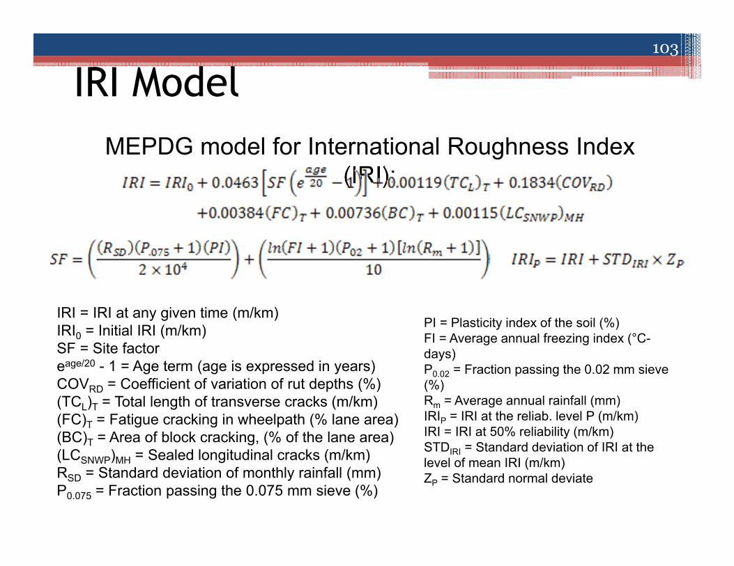
IRI ModelMEPDG model for International Roughness Index

(IRI):

IRI = IRI at any given time (m/km)IRI0 = Initial IRI (m/km)SF = Site factoreage/20 - 1 = Age term (age is expressed in years)COVRD = Coefficient of variation of rut depths (%)(TCL)T = Total length of transverse cracks (m/km)(FC)T = Fatigue cracking in wheelpath (% lane area)(BC)T = Area of block cracking, (% of the lane area)(LCSNWP)MH = Sealed longitudinal cracks (m/km)RSD = Standard deviation of monthly rainfall (mm)P0.075 = Fraction passing the 0.075 mm sieve (%)

PI = Plasticity index of the soil (%)FI = Average annual freezing index (°C-days)P0.02 = Fraction passing the 0.02 mm sieve (%)Rm = Average annual rainfall (mm)IRIP = IRI at the reliab. level P (m/km)IRI = IRI at 50% reliability (m/km)STDIRI = Standard deviation of IRI at the level of mean IRI (m/km)ZP = Standard normal deviate

103

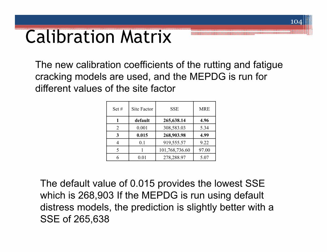
Calibration MatrixThe new calibration coefficients of the rutting and fatigue cracking models are used, and the MEPDG is run fordifferent values of the site factor

Set # Site Factor SSE MRE

1 default 265,638.14 4.962 0.001 308,583.03 5.343 0.015 268,903.98 4.994 0.1 919,555.57 9.225 1 101,768,736.60 97.006 0.01 278,288.97 5.07

The default value of 0.015 provides the lowest SSE which is 268,903 If the MEPDG is run using default distress models, the prediction is slightly better with a SSE of 265,638

104

The new rutting and fatigue cracking models and a Site Factor = 0.015 slightly increases the SSE from 265,638 to 268,903This model shows a good agreement

Results: IRI

0

50

100

150

200

250

300

0 50 100 150 200 250 300

Pred

icte

d IR

I (in

/mile

)

Measured IRI (in/mile)

LTPP Sections

NMDOT Sections

0

50

100

150

200

250

300

0 50 100 150 200 250 300Pr

edic

ted

IRI (

in/m

ile)

Measured IRI (in/mile)

LTPP Sections

NMDOT Sections

Uncalibrated

Calibrated

105

IRI Validation

Sections 1112, 2007, NMDOT 5, NMDOT 6, and NMDOT 10 are kept aside for validation. The MEPDG prediction barely varies with the new model, the SSE

slightly increases from 7,472.85 to 8,106

0

20

40

60

80

100

120

140

160

0 5 10 15 20 25

IRI (

in/m

ile)

Design Life (years)

Measured

Uncalibrated

Calibrated

NMDOT 6

106

Summary of Local Calibration

• Rutting: βr1 = 1.1, βr2 = 1.1, βr3 = 0.8, βGB = 0.8, βSG = 1.2

• Alligator Cracking: C1 = 0.625, C2 = 0.25, C3 = 6000

• Longitudinal Cracking: C1 = 3, C2 = 0.3, C3 = 1000

• IRI: Site Factor = 0.015

107

Implementation Note

• MEPDG database work needs to be continued

• The sets of calibration coefficients obtained for the MEPDG permanent deformation, fatigue cracking and IRI models can reduce the error in the prediction, and thus, be beneficial for pavement design.

• Improvement is still possible to achieve in the future

108

Documents

Development of a Flexible Pavement Database for Local ...dot.state.nm.us/content/dam/nmdot/Research/MultimediaPresentationM...NMDOT Design Method AASHTO 1972 for Pavement Design with